Evaluating the Robustness of Zero-Shot Time Series Models Against Data Degradation in Industrial Sensor Streams

Abstract

Zero-shot time series foundation models (TSFMs) forecast unseen series without target-specific training, offering a way to significantly reduce the deployment overhead in enterprise pipelines and industrial sensor streams. However, their performance is documented almost exclusively on pristine benchmarks, whereas industrial data streams feature missing values, sensor outages, and amplitude spikes. Whether these models absorb such faults natively, and thus whether costly imputation stages can be removed, remains unquantified. In this study, we evaluate the robustness of three TSFMs from distinct architectural families, Chronos (tokenization), TimesFM (patching), and TiRex (xLSTM), subjecting their context windows to random missing data, contiguous block missingness, and injection of point anomalies at escalating severities and assessing point accuracy (relative RMSE) and $80\%$ interval reliability (PICP) against a clean baseline. The results show that random dropout and transient spikes are natively absorbed by all three models (accuracy loss below $3\%$), while sustained contiguous outages are the dominant failure mode, with patch-based TimesFM most exposed (up to $59\%$). TiRex stays well calibrated throughout, while tokenization-based Chronos yields persistently overconfident intervals. These patterns persist and the contiguous outage vulnerability is amplified on data with genuine operational anomalies. For the evaluated models, sensor streams, and tested corruption severities, the results indicate that direct inference remains close to the clean-context baseline under independent random loss and sparse positive spikes, whereas prolonged outages warrant additional missing-data handling.

1. Introduction

Time series forecasting is a critical component of enterprise data architectures, driving automated decision-making across many domains [1]. In industrial environments such as manufacturing, smart grids, and process control, thousands of high-frequency sensors are deployed continuously [2]. Traditionally, maintaining predictive pipelines at this scale requires training and updating task-specific models for individual sensor channels, an approach that is computationally prohibitive and operationally unscalable [3]. Recently, however, the field has undergone a paradigm shift. Inspired by the architectural successes of Large Language Models (LLMs), researchers have developed zero-shot time series foundation models (TSFMs) that rely on cross-domain pre-training over large corpora of heterogeneous observations [4].

To achieve generalization, TSFMs adopt novel structural mechanisms to map continuous temporal dynamics into highly expressive representation spaces. For example, some models quantize sequences into discrete tokens [5], whereas others employ patch-based attention layers to efficiently capture local semantic dependencies across varying sampling frequencies [6]. By internalizing universal temporal priors such as seasonality, trend, and variance during pre-training, TSFMs can align an entirely unseen sequence to their learned distributions and extrapolate future horizons without target-specific fine-tuning [7]. This zero-shot capability is highly attractive for data engineers looking to streamline data pipelines, reduce deployment overhead, and rapidly onboard new sensor streams.

However, a significant gap exists between the pristine datasets used to benchmark TSFMs and the operational reality of industrial data. In production, time series are rarely perfect. Industrial Internet of Things (IIoT) networks operate in harsh conditions: hardware degrades, battery depletion causes sensor outages, network latency leads to dropped packets, and electromagnetic interference introduces severe amplitude spikes [8,9]. Consequently, context windows frequently contain randomly missing data, contiguous blocks of null values, and transient noise [10]. When a forecasting model is overly sensitive to such degradation, it can produce erratic predictions that trigger false alarms or cause downstream automated control systems to fail. While the performance of TSFMs is well documented under ideal conditions, their structural resilience to degraded context windows remains largely unquantified.

This uncertainty presents an architectural dilemma. Industrial data pipelines commonly span data acquisition, cleaning, integration, and analytics stages, with missing-value handling typically located within the cleaning stage [11,12]. Traditional forecasting pipelines may therefore apply imputation or smoothing before inference when data are incomplete or noisy [13]. If modern TSFMs remain accurate when degradation is passed directly to their inference interfaces, practitioners may be able to simplify this preprocessing stage in suitable deployments. In turn, the importance of minimizing such computational overhead extends beyond operational efficiency. As recent studies in complex data processing highlight, optimizing algorithms to reduce unnecessary computation is increasingly necessary to mitigate the energy consumption and environmental impact of enterprise data architectures [14]. The present study examines this question through direct robustness relative to clean-context inference.

As our operational question is whether TSFMs can safely bypass explicit imputation, we benchmark their structural resilience against their own pristine baselines rather than classical statistical methods. We examine whether the evaluated models, which use distinct temporal representations and inference pathways, exhibit different vulnerabilities to data corruption. For instance, discrete tokenization might inherently filter out minor noise through binning, while continuous patching might be uniquely exposed to contiguous outages. We evaluate three zero-shot TSFMs under simulated data degradation in a continuous streaming mode. We focus on high-frequency industrial sensor streams using the SKAB suite, which provides distinct channels and pairs clean data with genuine operational faults. We select one representative model for each broad design approach, discrete tokenization (Chronos), continuous patching (TimesFM), and xLSTM-based recurrence (TiRex), and subject their context windows to three escalating degradation profiles. This design enables a practical comparison of three released zero-shot TSFM configurations, rather than an isolation of the encoding strategy alone.

The primary contributions of this paper are as follows:

• An empirical quantification of how random missing data ($5\%$, $10\%$, $20\%$) impacts the predictive accuracy and uncertainty estimation of TSFMs.
• An evaluation of model resilience to temporal data unavailability, simulated via contiguous block missingness of varying durations (100, 200, and 400 datapoints) within the context window.
• A robustness assessment against transient temporal noise, measuring degradation when $1\%$ of the context is corrupted by amplitude spikes of 2, 3, and 5 standard deviations.
• Evidence-based guidelines for data engineers, identifying where costly imputation pipelines can be safely bypassed in favor of raw data ingestion.

The rest of this paper is organized as follows. Section 2 provides the background and related work. Section 3 describes the problem formulation and methodology. Section 4 provides a comprehensive discussion of the experimentation and its results. Section 5 concludes and outlines future work.

2. Background and Related Work

This section provides a background on the evolution of zero-shot time series forecasting and positions our study within the related work.

2.1. From Task-Specific Models to Foundation Models

Deep learning first improved on classical statistical forecasting through task-specific architectures. Hybrid designs such as ES-RNN [15] combined exponential smoothing with recurrent networks, while N-BEATS [16] showed that a deep residual MLP could outperform established statistical baselines. The subsequent adaptation of self-attention to temporal data, including Informer [17], Autoformer [18], and PatchTST [19], extended these gains by capturing long-range dependencies within historical context windows. These architectures share one constraint. Specifically, each must be trained on its target dataset before producing accurate forecasts. Large-scale, cross-domain pre-training removed this requirement and gave rise to zero-shot TSFMs, which forecast previously unseen series without any weight updates [4]. Our work builds on this line of research but shifts the question from how well TSFMs forecast clean data to how their underlying structure behaves when the context window is degraded.

2.2. Zero-Shot Time Series Foundation Models

TSFMs differ in how they encode the context window before forecasting, and classifying them by this design choice clarifies how each distributes attention across historical data. We identify three broad families.

• Discrete tokenization. This family treats forecasting as a sequence-modeling problem over a discrete vocabulary, enabling the direct transfer of LLM training paradigms and scaling laws to temporal data. Chronos [5] scales and quantizes continuous values into a fixed token vocabulary, reusing language-model tooling through a T5 encoder–decoder backbone to learn distributions over discrete temporal states. TOTEM [20] follows the same philosophy but learns its vocabulary with a vector-quantized autoencoder rather than fixed binning and then models sequences of the resulting code with a transformer. Expanding on this approach, LLMTime [21] directly encodes numerical sequences as discrete text strings; by relying entirely on the native subword tokenization of off-the-shelf language models, it harnesses existing text-based probability distributions to perform zero-shot forecasting without requiring domain-specific structural modifications.
• Continuous patching. The next family projects continuous values directly, grouping consecutive observations into patches. This reduces the effective sequence length, easing the quadratic memory bottleneck of traditional self-attention while preserving local semantic structures. TimesFM [6] embeds fixed-length patches and decodes future patches autoregressively, reducing attention cost and capturing local structure before modeling long-range dependencies. In turn, Moirai [22] extends this with a masked-encoder design that combines multiple patch sizes and an any-variate attention mechanism to handle varying frequencies and dimensionalities. Moreover, Toto [23] embeds per-series-scaled segments and forecasts through a Student-t mixture output head rather than a discrete vocabulary. Emphasizing efficiency, Tiny Time Mixers (TTMs) were introduced by Ekambaram et al. [24] as a lightweight model architecture that combines adaptive patching, diverse resolution sampling, and resolution prefix tuning, demonstrating that continuous patching can achieve zero-shot accuracy competitive with massive LLMs at a fraction of their parameter count.
• Beyond the transformer. This group departs from the transformer-token paradigm entirely, seeking to capture long-range dependencies without the steep computational scaling of self-attention. TiRex [25] adopts a recurrent xLSTM architecture, using patched inputs and quantile outputs to produce probabilistic forecasts. In turn, Sundial [26] pairs continuous patch tokenization with a generative flow-matching output head. Adding to this architectural shift, State Space Models (SSMs) such as TimeMachine [27] leverage Mamba architectures to achieve linear time complexity; this allows them to ingest highly extended historical context windows while maintaining constant memory bounds during inference. These encoding choices govern how each model weights its context, and we argue that they also shape their sensitivity to corrupted inputs, a relationship that has not been directly quantified. This observation motivates our selection of one representative per family in the evaluation that follows.

Recent evidence also shows that zero-shot TSFM evaluation should consider both point accuracy and probabilistic reliability. Michael et al. [28] benchmark several TSFMs across energy, traffic, and financial datasets, identifying a trade-off between point forecasting accuracy and interval calibration that varies across model configurations and forecast horizons. Complementing this broader clean-data evaluation, our study examines how point accuracy and interval reliability change when industrial sensor contexts are degraded.

2.3. Robustness to Corrupted Context Windows

How forecasting models behave on imperfect context windows is a central data-engineering concern, yet most evidence still comes from earlier transformer studies rather than from zero-shot TSFMs. As self-attention computes pairwise similarities across the sequence, a single large amplitude spike can dominate the softmax distribution and starve the remaining context of attention weights, skewing the forecast horizon [29]. Consistent with this, Zeng et al. [30] show that transformer forecasters can degrade sharply under temporal noise, at times trailing simple linear baselines once data quality falls.

Incomplete windows raise a distinct problem. Fixed positional encodings and standard attention assume uniform sampled inputs, so dropouts and contiguous gaps corrupt the learned temporal representation and reduce accuracy [10]. The remedy is computationally expensive imputation prior to inference, such as self-attention-based reconstruction, where missing gaps are filled before data reaches the forecasting module [13].

Recent benchmarking efforts continue to evaluate these standard imputation strategies across different domains. For example, Toye et al. [31] investigate the effects of randomly missing data alongside non-random missingness, relying on clean baseline segments extracted from two medical datasets to simulate degradation and measure imputation error. Similarly, Zhou [32] examines randomly missing data (Missing Completely At Random), which aligns with our focus on random loss, while also addressing complex non-random missing mechanisms. However, a distinct difference in scope exists: Toye et al. focus on medical records, and Zhou evaluates generative and kernel-based imputation techniques primarily on heterogeneous tabular benchmark datasets (e.g., Adult, California Housing). Both studies focus on optimizing explicit imputation steps. Whether the large-scale pre-training of zero-shot TSFMs lets them absorb such faults natively in industrial settings, bridging missing blocks and discounting amplitude spikes without external preprocessing, remains largely untested, since their resilience is documented almost exclusively on pristine benchmarks. Closing this gap addresses the evidence practitioners’ need to decide whether to maintain imputation pipelines or ingest raw, degraded data directly, which is the question this paper addresses.

3. Problem Formulation and Methodology

This section establishes the formal framework for time series forecasting and describes the synthetic degradation pipelines used to benchmark zero-shot TSFMs.

3.1. Streaming Context Window Formulation

In a production streaming environment, a continuous univariate time series is ingested sequentially. Let the continuous stream be defined as a sequence of real-valued observations $S=\{x_1,x_2,\dots ,x_N\}$. For the purposes of this benchmarking study, each complete time series is evaluated using a sliding window approach. At any forecast origin t, the series is partitioned into a historical context window $C_t$ of fixed length L and a subsequent forecast horizon $Y_t$ of length H. The context window is extracted as follows:

$$C_t=\{x_{t-L+1},x_{t-L+2},\dots ,x_t\}$$

The objective of the zero-shot time series forecasting model f is to process the context window $C_t$ and predict the horizon $Y_t$, as follows:

$${\widehat{Y}}_t=f\left(C_t\right)=\{{\widehat{y}}_{t+1},{\widehat{y}}_{t+2},\dots ,{\widehat{y}}_{t+H}\}$$

After a prediction based solely on the knowledge contained within $C_t$, the system slides forward through the data to form the next $C_t$.

This rolling mechanism allows us to perform multiple distinct predictions across the entire dataset, generating a comprehensive performance profile.

Throughout this iterative process, the following occur:

• All models operate in a strict zero-shot mode;
• The models do not receive any parameter updates as the window advances;
• No external imputation modules are applied prior to inference;
• The corrupted context window is passed directly to the model to assess its native structural resilience.

3.2. Data Degradation Scenarios

To simulate real-world data-engineering failures, we introduce three distinct degradation pipelines applied exclusively to each context window $C_t$. We explicitly denote that the ground-truth forecast horizon $Y_t$ is not altered for evaluation purposes, as the focus is entirely on how the historic context alteration affects the predictive ability of zero-shot TSFMs.

3.2.1. Random Point Missingness (RPM Scenarios)

To evaluate the models’ robustness to random datapoint loss (e.g., temporal sensor failure), we simulate data missing from the current $C_t$ at random time steps. We define a binary masking vector $M=\{m_1,\dots ,m_L\}$, where each element is drawn from a Bernoulli distribution. The probability of an element being dropped is defined by the missing data rate, denoted as $\rho$:

$$P(m_i=0)=\rho$$

Each observation is dropped independently with probability $\rho$, so the number of missing points per window is not fixed but varies around its expected value $\rho ·L$. We benchmark the models across three specific degradation thresholds: $\rho \in \{0.05,0.10,0.20\}$. Towards this, the corrupted context window ${\tilde{C}}_t$ is then obtained by replacing every observation, denoted as ${\tilde{x}}_i$, at a masked position ($m_i=0$) with the missing-value marker Not a Number (NaN):

$${\tilde{x}}_i=\left\{\begin{array}{cc}{x}_i\hfill & \mathrm{if}{m}_i=1\hfill \\ \mathtt{NaN}\hfill & \mathrm{if}{m}_i=0.\hfill \end{array}\right.$$

The NaN marker is used by the common corruption generator to denote absent observations. Before inference, a thin model-specific adapter translates this shared missingness pattern into the input representation required by each model’s official inference interface. The adapters do not interpolate, smooth, or otherwise reconstruct missing observations. Chronos-2 natively accepts a context-validity mask and can construct this mask from NaN entries. TiRex uses its native value-and-mask representation, in which missing observations are zero-filled and accompanied by a binary indicator mask. For TimesFM-2.5, the adapter supplies the model’s native padding mask together with the corresponding input tensor. Thus, the benchmark evaluates the end-to-end behavior of the released model configurations under a common corruption pattern, including their respective missing-value input interfaces, rather than isolating the forecasting backbone architecture from its missing-data-handling mechanism.

3.2.2. Contiguous Block Missingness (CBM Scenarios)

Intermittent random missingness does not capture events such as hardware outages or prolonged network disconnections where a contiguous block of datapoints can be missing in a context window.

To benchmark this, we introduce CBM scenarios. For a context window of length L, we define a failure block of length B, testing three distinct outage durations: $B\in \{100,200,400\}$ datapoints. For every context window and independent repetition, a starting index j is sampled uniformly from the set of valid positions $\{1,\dots ,L-B+1\}$. The missing block can therefore occur near the beginning, middle, or end of the historical context, including positions immediately preceding the forecast origin.

All sequential observations from $x_j$ to $x_{j+B-1}$ within the context window $C_t$ are then replaced with the missing-value marker NaN, consistent with the previous scenario. Randomizing the block position avoids assuming a particular outage location and yields a location-agnostic estimate of robustness to sustained data unavailability. Accordingly, the reported results summarize average behavior across possible gap placements rather than isolating the effect of a gap at one fixed temporal position. This tests whether the foundation models can bridge large, contiguous temporal gaps without explicit linear interpolation or spline imputation.

3.2.3. Point Anomaly Injection (PAI Scenarios)

Data pipelines frequently suffer from transient positive amplitude spikes (outliers) caused by calibration errors or external interference. To evaluate model sensitivity to this temporal noise, we inject artificial amplitude spikes into approximately 1% of the observations within the given context window. We deliberately keep this fraction low so that the spikes act as sparse point anomalies rather than a systematic shift in the window’s amplitude distribution, which would otherwise alter the statistical regime the model conditions on rather than test its resilience to isolated outliers.

Let ${\sigma }_C$ denote the standard deviation of the current context window $C_t$. We select a random subset of indices A, where the cardinality $\left|A\right|=\lceil 0.01·L\rceil$. We take the ceiling so that at least one point is perturbed when $0.01·L$ is non-integer. For each index $i\in A$, the original datapoint $x_i$ is perturbed by adding an artificial spike scaled by a severity multiplier k:

$${\tilde{x}}_i=x_i+(k·{\sigma }_C)$$

We benchmark the models against three escalating anomaly severities, testing spikes scaled at 2, 3, and 5 standard deviations (where $k\in \{2,3,5\}$). The perturbations are positive by design, so that anomaly direction remains fixed while severity increases. This provides a controlled comparison of sensitivity to sparse transient amplitude excursions across models and scenarios. The protocol is therefore not a sign-symmetric anomaly test, and its findings should be interpreted as applying to the evaluated positive-spike mechanism rather than to negative or mixed-sign point anomalies.

The three scenarios form a controlled and representative fault suite rather than an exhaustive taxonomy of industrial data degradation. RPM models independent random observation loss, CBM models sustained contiguous outages, and PAI models sparse positive amplitude excursions. For CBM, the block start index is sampled uniformly from all valid locations for every context window and repetition, so the evaluation aggregates varying gap positions rather than fixing an outage at one point in the context. Accordingly, the conclusions of this study are bounded to the tested corruption mechanisms and severities. Negative point perturbations, missingness processes conditional on signal values or operating state, and other structured degradation patterns are not evaluated in the present benchmark.

3.3. Evaluated Models

We evaluate three zero-shot TSFMs, each drawn from one of the architectural families introduced in Section 2: Chronos-2 (discrete tokenization), TimesFM-2.5 (continuous patching), and TiRex (non-transformer, xLSTM). For all TSFMs, we use their latest released checkpoints and the same architectures described in Section 2. Key configurations of each model are presented in Table 1. We denote once again that the selected models differ in more than their broad temporal design approach, including their pre-training data, parameter counts, output heads, scaling procedures, and native missing-value input pathways. The comparison should therefore be interpreted as an end-to-end evaluation of these three released model configurations. References to tokenization, patching, and xLSTM recurrence provide architectural context for the observed patterns but do not isolate architecture as their sole cause.

Table 1. Configuration of the evaluated zero-shot TSFMs. All models use official HuggingFace checkpoints, emit $0.1/0.5/0.9$ quantiles, and run without fine-tuning.

	Chronos-2	TimesFM-2.5	TiRex
Release version	2.3.0	2.0.1	1.4.2
Family	Tokenization	Patching	xLSTM
Parameters	∼120 M	∼200 M	∼35 M
Input format	(id, ts, target)	tensor	tensor (batch × context)
Context L	600	600	600
Pred. length	60	60	60
Quantiles	0.1, 0.5, 0.9	0.1, 0.5, 0.9	0.1, 0.5, 0.9
Fine-tuning	No	No	No

Moreover, for each model, we use the official pre-trained weights released on Hugging Face, and all models run strictly in zero-shot mode with no fine-tuning or parameter updates. The comparative results should therefore be interpreted as the robustness of each released model and its official inference pathway, including its native missing-value representation, rather than as an isolation of backbone architecture alone.

3.4. Datasets and Evaluation Metrics

The following datasets and evaluation metrics are used during the evaluation process of our study.

3.4.1. Datasets

The TSFMs selected for the benchmarking process are evaluated on the Skoltech Anomaly Benchmark (SKAB) [33], a benchmark suite comprising several distinct datasets of multivariate sensor recordings collected from an industrial water-circulation testbed. We draw on two test modes of this suite.

First, we use the anomaly-free datasets as a controlled baseline. As these recordings contain no native faults, any degradation in forecasting performance can be attributed directly to our injected scenarios rather than to pre-existing irregularities in the data. Second, we use the valve1 collection, whose recordings contain genuine anomalies arising from the industrial process, allowing us to assess how the degradation scenarios interact with real operational conditions rather than with synthetically clean signals alone.

For each dataset, every available sensor channel is treated as an individual univariate time series and evaluated under the described protocol, so that our results reflect performance across the full set of measured variables. The sensor channels are denoted as Accelerometer1RMS, Accelerometer2RMS, Current, Pressure, Temperature, Thermocouple, Voltage, and RateRMS.

The SKAB recordings are sampled at 1 Hz (one observation per second), which fixes the physical scale of our streaming protocol. We set the context window to $L=600$ observations, corresponding to 10 min of recent sensor history, and the forecast horizon to $H=60$ observations, corresponding to the subsequent 1 min. This configuration represents a short-horizon industrial forecasting setting in which recent operating dynamics are relevant while maintaining a common context length supported by all evaluated models. To keep the evaluation computationally tractable while preserving repeated coverage of each stream, the window advances with a step of 120 observations, producing a new forecast origin every 2 min. These choices also define the relative severity of contiguous outages. The evaluated CBM blocks of 100, 200, and 400 observations correspond to approximately 2, 3, and 7 min of missing data, or $16.7\%$, $33.3\%$, and $66.7\%$ of the 10 min context window, respectively. Consequently, the absolute impact of a fixed-duration outage may differ under another context length or forecast horizon. Within this study, however, all models are evaluated using the same context, horizon, sliding step, and relative outage proportions, allowing their robustness to be compared consistently under the defined streaming configuration.

3.4.2. Evaluation Metrics

To quantify forecasting error under degradation, we evaluate the point predictions against the clean horizon $Y_t$ of length H using the Root Mean Squared Error (RMSE), which penalizes the large mispredictions that data degradation can induce:

$$\mathrm{RMSE}=\sqrt{{\displaystyle \frac{1}{H}}\sum _{h=1}^H{(y_{t+h}-{\widehat{y}}_{t+h})}^2}$$

The absolute scales of the SKAB channels differ by several orders of magnitude. In the clean reference, RMSE ranges from approximately $0.0018$ on the accelerometer channels to roughly 11 on the voltage channel. Averaging these raw values would let a single high-magnitude channel dominate the aggregate. To place all channels on a common scale, we report RMSE as its relative degradation with respect to each channel’s own clean baseline:

$$\mathsf{\Delta }\mathrm{RMSE}\%={\displaystyle \frac{{\mathrm{RMSE}}_{\mathrm{scenario}}-{\mathrm{RMSE}}_{\mathrm{clean}}}{{\mathrm{RMSE}}_{\mathrm{clean}}}}\times 100$$

A value of 0 indicates no change from the baseline and larger positive values indicate stronger degradation, while small negative values can occur when a model fits a noisy window marginally better than the clean one. As this quantity is dimensionless, the eight sensor channels are directly comparable.

To assess probabilistic forecasts, we evaluate the $80\%$ prediction interval formed by the 10th and 90th percentile forecasts (${\widehat{y}}^{\left(0.1\right)}$, ${\widehat{y}}^{\left(0.9\right)}$) using the Prediction Interval Coverage Probability (PICP), the proportion of true observations falling within the predicted bounds:

$$\mathrm{PICP}={\displaystyle \frac{1}{H}}{\displaystyle \sum _{h=1}^H}\mathbf{1}\{{\widehat{y}}_{t+h}^{\left(0.1\right)}\le y_{t+h}\le {\widehat{y}}_{t+h}^{\left(0.9\right)}\}$$

where $\mathbf{1}$ is the indicator function. A well-calibrated model should achieve a PICP close to the nominal $0.80$. Since PICP already lies on a common 0-to-1 scale across channels, we report it directly, both as absolute coverage and as its deviation from the nominal target ($\mathsf{\Delta }\mathrm{PICP}={\mathrm{PICP}}_{\mathrm{scenario}}-0.80$).

4. Evaluation

This section reports our findings in two stages. We first establish a clean reference on the SKAB anomaly-free subset, and then inject each degradation scenario at escalating severity, quantifying the effect on point accuracy (Section 4.1) and interval calibration (Section 4.2). As the baseline series carry no native faults, any movement relative to the clean reference is attributable to the injected corruption alone. Section 4.3 then examines whether the patterns observed under controlled, synthetic degradation persist on the valve1 datasets, whose series contain genuine operational anomalies.

As all three degradation pipelines involve randomness, namely the masked positions for RPM, the contiguous-block start index for CBM, and the perturbed indices for PAI, we repeat every scenario 11 times with independent draws. Each realization is evaluated over all rolling forecast origins and the eight sensor channels. For a given scenario, the same generated corruption pattern is applied to Chronos-2, TimesFM-2.5, and TiRex. Thus, model comparisons are paired with respect to the locations of dropped observations, missing blocks, or injected anomalies. We use an odd number of realizations so that the median corresponds to an observed run. To summarize a model–scenario pair, we rank the runs by their across-channel mean $\mathsf{\Delta }$RMSE% and report the median realization. This provides a representative corruption draw, avoids results being determined by an unusually favorable or unfavorable placement, and retains the associated point-forecast and interval-calibration outcomes from the same realization.

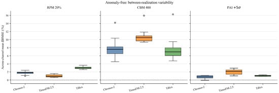
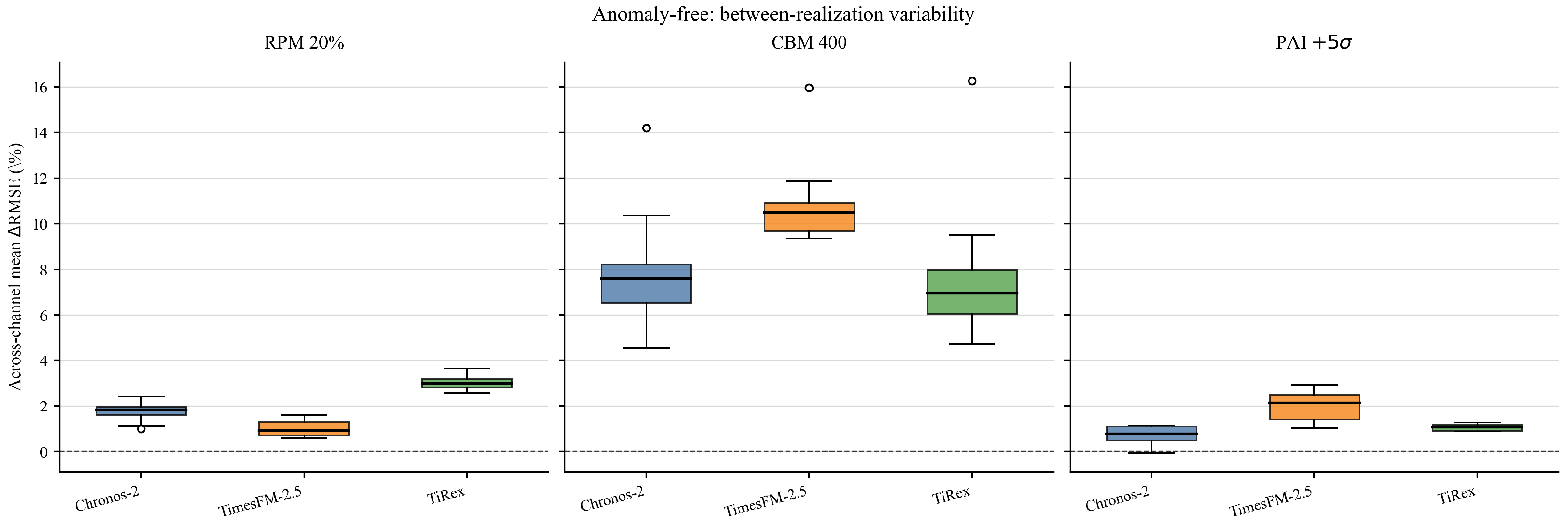
To supplement the representative-realization results, boxplots are used to show run-to-run variability for the highest tested severity of each degradation mechanism: RPM 20%, CBM 400, and PAI $+5\sigma$. In brief, the boxplots display the median and interquartile range; points beyond the whiskers indicate outliers. These plots complement the across-channel ranges in Table 2 and Table 3, which describe variation across sensor channels for the reported representative realization.

Table 2. Robustness summary per scenario (median of 11 runs): $\mathsf{\Delta }$RMSE% against each channel’s clean baseline (left) and $\mathsf{\Delta }$PICP deviation from the $80\%$ target (right). Each cell is the across-channel mean with the $[\min ,\max ]$ over the eight channels.

	Point Accuracy ($\mathbf{\Delta }$RMSE%)			Interval Reliability ($\mathbf{\Delta }$PICP)
Scenario	Chronos-2	TimesFM-2.5	TiRex	Chronos-2	TimesFM-2.5	TiRex
RPM 5%	+0.9% [−1.6, +8.1]	+0.2% [−1.5, +3.0]	+0.8% [−1.5, +6.7]	−3.0 [−6.6, 0.0]	−0.9 [−3.2, +3.3]	−0.3 [−2.3, +2.0]
RPM 10%	+1.3% [−1.3, +10.9]	+0.4% [−1.7, +3.2]	+1.9% [−3.7, +12.1]	−3.4 [−7.6, −0.2]	−1.4 [−3.5, +3.5]	−0.8 [−3.7, +0.8]
RPM 20%	+1.8% [−1.5, +11.0]	+1.0% [−2.7, +5.9]	+3.0% [−3.0, +17.2]	−4.0 [−8.8, −1.1]	−2.1 [−5.1, +3.7]	−1.1 [−5.1, +0.8]
CBM 100	+1.1% [−3.9, +11.1]	+2.7% [−2.1, +13.1]	+1.2% [−4.0, +9.2]	−2.7 [−8.8, +0.7]	+0.3 [−2.8, +3.4]	+0.7 [−3.5, +6.4]
CBM 200	+2.7% [−0.6, +21.6]	+5.3% [−3.1, +23.7]	+3.1% [−2.1, +15.8]	−2.8 [−9.1, +1.8]	−0.1 [−4.9, +4.6]	+0.8 [−3.2, +6.6]
CBM 400	+8.0% [−1.3, +44.1]	+11.1% [−4.1, +59.0]	+7.8% [−0.6, +41.7]	−2.6 [−8.4, −0.2]	−0.3 [−10.8, +6.4]	+0.7 [−3.1, +5.0]
PAI +2$\sigma$	+0.5% [−1.6, +6.2]	+0.6% [−2.1, +6.0]	+0.3% [−0.9, +1.7]	−1.8 [−7.1, +3.1]	+0.6 [−1.6, +6.1]	+1.5 [−1.6, +7.7]
PAI +3$\sigma$	+0.5% [−1.9, +5.6]	+1.3% [−1.5, +14.3]	+0.6% [−0.2, +3.1]	−1.4 [−7.0, +3.3]	+1.2 [−1.4, +7.3]	+1.8 [−1.5, +8.3]
PAI +5$\sigma$	+0.8% [−1.3, +9.5]	+2.2% [−1.4, +18.6]	+1.1% [−0.4, +5.7]	−0.9 [−5.8, +4.0]	+1.6 [−1.3, +9.0]	+1.7 [−1.7, +8.0]

Table 3. Robustness summary for valve1 (median of 11 runs). $\mathsf{\Delta }$RMSE% against each channel’s own valve1 baseline (left) and $\mathsf{\Delta }$PICP deviation from the $80\%$ target (right). Each cell is the across-channel mean with the $[\min ,\max ]$ over the eight channels.

	Point Accuracy ($\mathbf{\Delta }$RMSE%)			Interval Reliability ($\mathbf{\Delta }$PICP)
Scenario	Chronos-2	TimesFM-2.5	TiRex	Chronos-2	TimesFM-2.5	TiRex
RPM 20%	+0.1% [−2.2, +2.6]	+0.2% [−2.2, +4.6]	+0.6% [−3.4, +3.3]	−1.2 [−11.3, +7.0]	−0.4 [−7.7, +15.7]	−0.5 [−13.0, +7.0]
CBM 100	−0.6% [−6.9, +4.7]	+0.7% [−5.7, +4.3]	+0.2% [−0.4, +1.1]	−0.3 [−11.3, +15.7]	+1.3 [−7.0, +16.3]	+2.7 [−2.3, +11.7]
CBM 200	+1.4% [−8.5, +16.8]	+3.4% [−3.8, +15.2]	+1.3% [+0.0, +3.6]	−0.5 [−13.3, +14.0]	+1.4 [−5.7, +18.3]	+3.0 [−3.0, +16.7]
CBM 400	+7.1% [+0.0, +24.8]	+17.4% [−0.1, +71.2]	+3.3% [−4.4, +13.7]	−1.1 [−9.7, +8.7]	−0.3 [−6.0, +6.0]	+2.8 [−2.3, +14.0]
PAI +5$\sigma$	−0.3% [−4.0, +2.9]	+2.5% [−0.3, +13.8]	−0.8% [−7.6, +0.4]	−0.7 [−8.7, +10.3]	+0.2 [−4.3, +4.0]	+3.2 [−3.7, +12.7]

Finally, we denote that per-realization outputs and the reproducibility notebook are provided to allow alternative aggregations, including medians with interquartile ranges or confidence intervals, to be derived without expanding the main result tables.

4.1. Point-Forecast Accuracy Under Context Degradation ($\mathsf{\Delta }$RMSE)

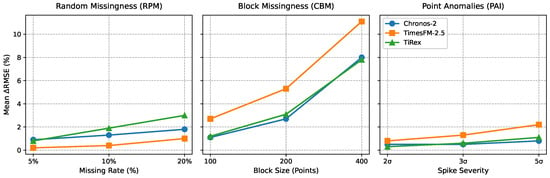
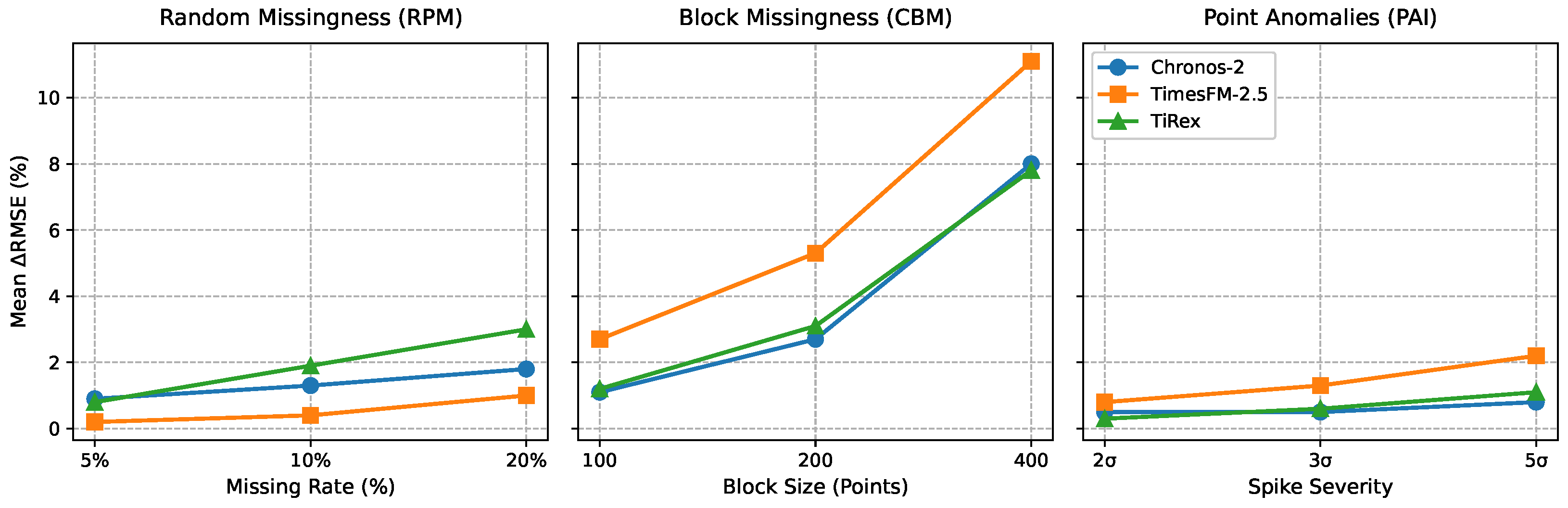
Table 2 summarizes the evaluation axes of the nine scenarios: relative point degradation ($\mathsf{\Delta }$RMSE%, left) and interval calibration ($\mathsf{\Delta }$PICP, right). Each cell reports the across-channel mean with its [min, max] range. Figure 1 and Figure 2 visualize the results per scenario. The analysis is descriptive, comparing cross-channel performance patterns across degradation scenarios and model architectures.

Figure 1. Mean relative forecasting error ($\mathsf{\Delta }$RMSE%) by degradation scenario.

Figure 2. Between-realization variability of $\mathsf{\Delta }$RMSE% for the highest tested severity of each degradation mechanism on the anomaly-free collection: RPM 20%, CBM 400, and PAI $+5\sigma$.

In the case of random missing datapoints, every model is broadly stable. Even at $20\%$ data loss, the average degradation stays modest, peaking at $+3.0\%$ for TiRex, and the marker-based NaN encoding lets each model treat dropped observations as absences rather than spurious zeros. TimesFM-2.5 is the most resilient, never exceeding $+1.0\%$ on average, with Chronos-2 close behind (rising from $+0.9\%$ to $+1.8\%$ as the rate climbs). TiRex shows the steepest average sensitivity ($+0.8\%$ to $+3.0\%$), and its per-channel spread is the widest: at $20\%$ missingness, its worst channel reaches $+17.2\%$, against per-channel maxima of $+11.0\%$ for Chronos-2 and $+5.9\%$ for TimesFM-2.5. The practical reading is that intermittent dropout does not meaningfully disturb the average forecast, though individual channels (most notably for TiRex) can still degrade noticeably.

Contiguous gaps are the dominant failure mode for every model. On average, degradation is mild for the 100- and 200-point blocks (at most $+5.3\%$) but escalates sharply at the 400-point outage. Here, TimesFM-2.5 degrades the most on average ($+11.1\%$), as erasing consecutive observations wipes out whole patch embeddings and leaves the local-attention map without an anchor, whereas Chronos-2 ($+8.0\%$) and TiRex ($+7.8\%$) hold up comparably better, consistent with discrete tokens and a recurrent xLSTM state bridging long gaps more gracefully. However, the per-channel ranges show that no architecture is safe: worst-channel degradation reaches $+59.0\%$ for TimesFM-2.5, $+44.1\%$ for Chronos-2, and $+41.7\%$ for TiRex. These peaks are amplified by relative normalization on low-variance channels (Pressure values between $-0.5$ and $0.5$), where a small clean-baseline RMSE inflates the percentage even when the absolute error stays modest. Hence, CBM is the scenario in which the encoding strategy matters most, with patch-based TimesFM-2.5 clearly the most exposed on average, yet the severe worst-channel degradation across all three models shows that sustained outages threaten every architecture (Figure 1).

Finally, the sparse positive amplitude spikes considered in the PAI protocol barely degrade point accuracy. Even at $5\sigma$ severity, the average degradation is at most $+2.2\%$, with Chronos-2 ($+0.8\%$) and TiRex ($+1.1\%$) essentially unaffected and TimesFM-2.5 the most sensitive ($+2.2\%$). Under the evaluated PAI protocol, the models largely absorb isolated positive outliers without explicit smoothing. In turn, the severe-case distributions in Figure 2 provide a run-level view of these point-forecast results. They show the spread of the across-channel mean $\mathsf{\Delta }$RMSE% across the available corruption realizations for each model. This complements the main tables by showing whether the reported model and scenario patterns are consistent across realizations or are accompanied by appreciable variation in the corruption draw.

Takeaway: For the evaluated zero-shot TSFMs and SKAB sensor streams, the independent random-dropout and sparse positive-spike scenarios can be ingested raw by TSFMs, since no model loses more than about $3\%$ average accuracy even at the highest tested severities. Explicit imputation earns its cost only for sustained outages: once a contiguous gap approaches a third or more of the context window, accuracy degrades most for patch-based TimesFM-2.5, while severe degradation on channels with small decimal ranges makes prolonged outages the one fault that no model absorbs reliably.

4.2. Interval Calibration Under Context Degradation (PICP)

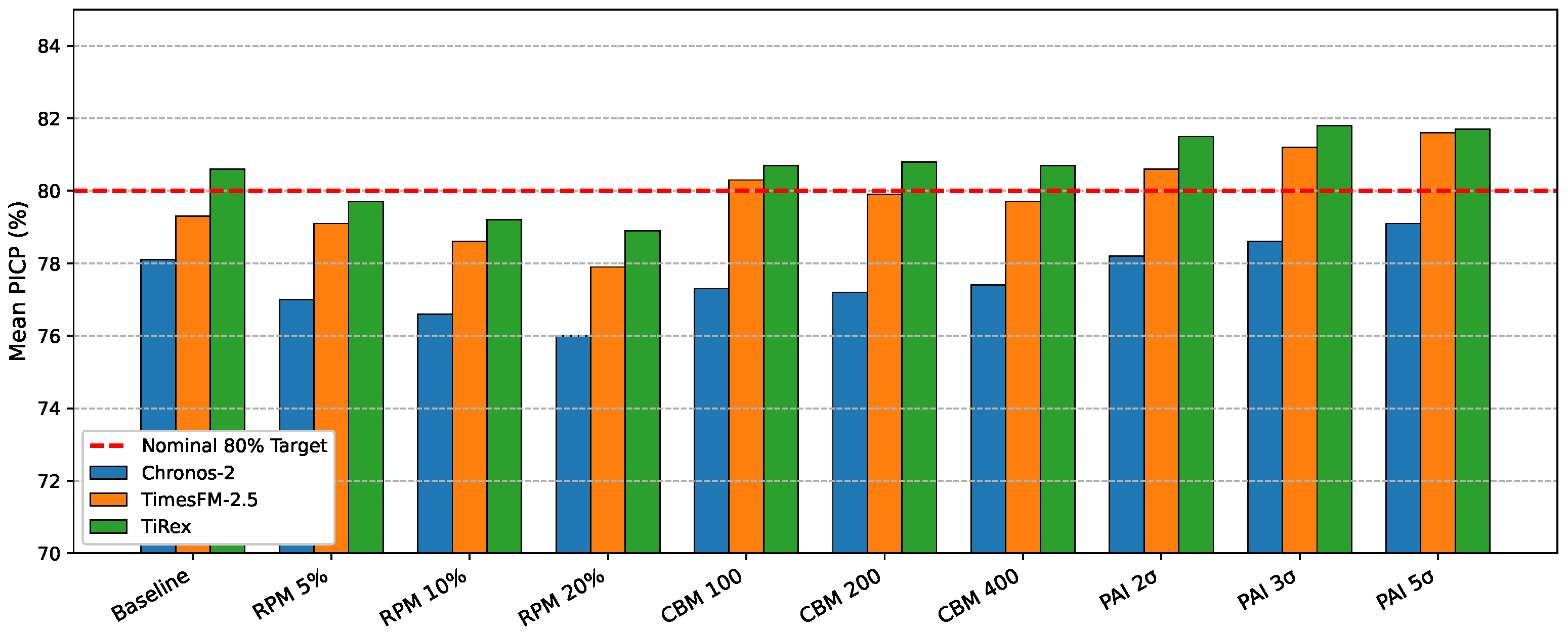
Assessed on the $80\%$ prediction interval (Figure 3), TiRex stays closest to the nominal target throughout, with average coverage between $78.9\%$ and $81.8\%$ across all scenarios. TimesFM-2.5 is also well calibrated, generally staying within about 2 percentage points of nominal (at worst $-2.1$, at $20\%$ missingness). Neither model shows systematic interval collapse under degradation, indicating that their uncertainty estimates remain trustworthy as the context deteriorates.

Figure 3. Prediction interval coverage (PICP) by scenario, with the dashed line denoting the $80\%$ nominal target.

In contrast, Chronos-2 consistently under-covers, sitting roughly 1 to 4 percentage points below the $80\%$ mark and falling to $76.0\%$ at $20\%$ random missingness ($\mathsf{\Delta }$PICP = −4.0). This under-coverage widens as missingness increases, indicating that the discrete tokenization strategy yields intervals that are too tight, and therefore overconfident, precisely when the input is least reliable.

The CBM scenarios reveal a useful decoupling between accuracy and calibration. Although CBM 400 inflicts the largest point-accuracy loss (Section 4.1), it barely disturbs interval coverage: TimesFM-2.5 stays within $0.3$ points of nominal ($\mathsf{\Delta }$PICP $=-0.3$) and TiRex even over-covers slightly ($+0.7$), while Chronos-2 holds its usual mild under-coverage ($-2.6$). In other words, the patch- and state-based models preserve trustworthy uncertainty estimates even where their point forecasts degrade sharply, so a downstream consumer reading the interval, rather than the point, is not misled by the outage.

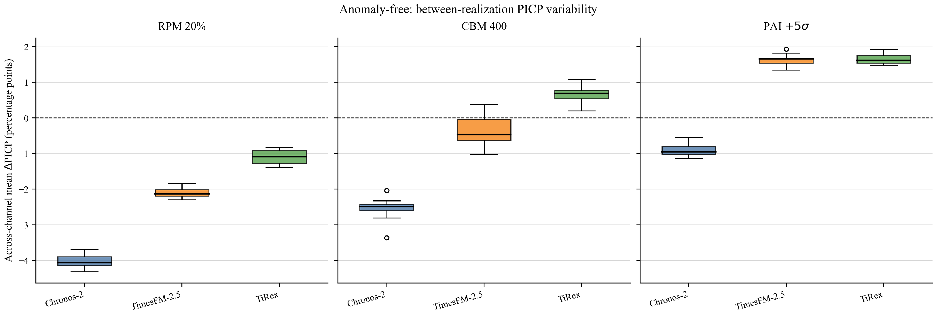
The PAI scenarios separate the families by their response to outliers. TiRex and TimesFM-2.5 correctly widen their intervals as spikes intensify, shifting $\mathsf{\Delta }$PICP positive (up to $+1.8$ for TiRex). Chronos-2 also improves under noise (from $-1.8$ at $2\sigma$ to $-0.9$ at $5\sigma$), but only as its baseline under-coverage is partly offset rather than because it adapts, and it still ends below nominal. Figure 4 shows the corresponding run-to-run distributions for $\mathsf{\Delta }$PICP. The boxplots indicate the median coverage deviation and its interquartile range across the available realizations for each model and severe scenario, complementing the representative-realization values reported in the main tables.

Figure 4. Between-realization variability of $\mathsf{\Delta }$PICP, in percentage points from the nominal $80\%$ target, for the highest tested severity of each degradation mechanism on the anomaly-free collection: RPM 20%, CBM 400, and PAI $+5\sigma$.

Takeaway: Degraded context does not break interval calibration for recurrent and patch-based models, which stay near-nominal and widen appropriately under noise. The exception is Chronos-2, whose tokenization yields overconfident intervals on clean, low-variance streams, and pipelines relying on its uncertainty estimates should apply a coverage correction in that regime.

4.3. Generalization to Data with Native Anomalies

The preceding analysis was conducted on data streams where the baseline was free of faults by construction. To assess whether the observed robustness patterns generalize beyond clean inputs, we extend the evaluation to the valve1 collection, whose recordings contain genuine operational anomalies, including cavitation, which produces high-frequency vibration on the accelerometer channels and an abrupt drop in RateRMS. We apply the identical degradation suite and protocol on each valve1 series and compute their $\mathsf{\Delta }$RMSE% and $\mathsf{\Delta }$PICP to retain the interpretation established in Section 4.1 and Section 4.2. This design isolates the effect of the injected corruption on data that already carries real faults, providing a direct test of the external validity of our findings.

Table 3 reports the valve1 results for the worst severity of RPM and PAI scenarios (RPM $20\%$, PAI $5\sigma$) together with all CBMs (100, 200, 400 points), since contiguous block missingness was the dominant failure mode on the clean data and therefore merits examination across its full range. We look for three patterns to recur: (i) contiguous block missingness remains the dominant failure mode, with mild degradation under RPM and PAI; (ii) the architectural ordering under CBM persists, with TimesFM-2.5 most exposed; and (iii) the Chronos-2 under-coverage persists or is specific to low-variance signals.

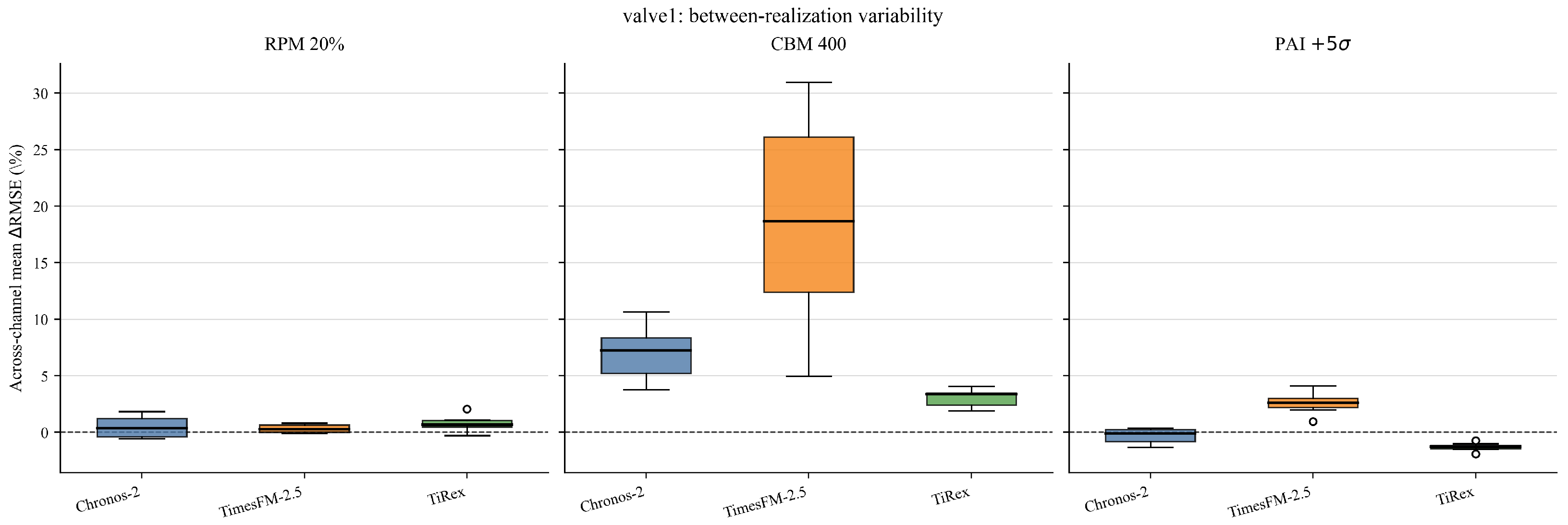
The valve1 results confirm the headline patterns and, for contiguous outages, sharpen them. Random missingness and the tested sparse positive point perturbations remain benign on data with native faults: every model stays within roughly $\pm 2.5\%$ $\mathsf{\Delta }$RMSE under both RPM $20\%$ and PAI $5\sigma$, and several values are mildly negative (Chronos-2 at $-0.3\%$ and TiRex at $-0.8\%$ under PAI), indicating that injected spikes do not compound the genuine anomalies already present. Contiguous block missingness again dominates, and the architectural ordering persists and in fact widens. On valve1, CBM degradation stays negligible at 100 and 200 points (average $\mathsf{\Delta }$RMSE at most $+3.4\%$) and escalates at 400, where TimesFM-2.5 rises to $+17.4\%$, well above its clean-baseline $+11.1\%$, while TiRex degrades less than on the clean data ($+3.3\%$ versus $+7.8\%$) and Chronos-2 is essentially unchanged ($+7.1\%$ versus $+8.0\%$). TimesFM-2.5 is the most exposed model at every CBM severity, confirming the ordering is not an artifact of the extreme block alone. The patch-erasure vulnerability and the xLSTM bridging advantage are therefore amplified, not masked, when the underlying signal already carries real anomalies, confirming patterns (i) and (ii) on operational data.

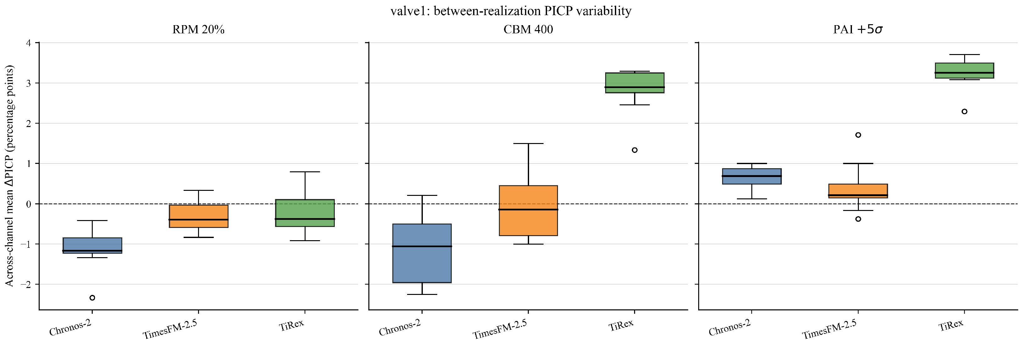
The calibration picture shifts more substantially. On the clean data, Chronos-2 is persistently overconfident, but on valve1, its under-coverage shrinks markedly: the deficit falls from $-4.0$ (clean RPM $20\%$) to between $-1.2$ and $-0.3$ across scenarios, no longer the systematic 1-to-4-point gap seen on clean streams. TiRex moves the other way, drifting to mild over-coverage under the harsher scenarios ($+2.8$ under CBM 400; $+3.2$ under PAI $5\sigma$), while TimesFM-2.5 stays near-nominal throughout ($-0.4$ to $+1.4$). The native variability of the valve1 signal appears to widen every model’s intervals, which offsets the structural tightness that tokenization exhibits on clean, low-variance data. Pattern (iii) therefore does not carry over cleanly: Chronos-2’s overconfidence is best read as an artifact of low-variance channels rather than a persistent property, and no model is meaningfully overconfident on real-anomaly data.

Finally, Figure 5 and Figure 6 show the between-realization variability on the valve1 collection for the highest tested severity of each degradation mechanism: RPM 20%, CBM 400, and PAI $+5\sigma$. Each box represents the across-channel mean for one stochastic realization. The plots complement Table 3 by showing the distribution of these results across realizations, including the median, interquartile range, and any outlying realizations.

Figure 5. Between-realization variability of $\mathsf{\Delta }$RMSE% for the highest tested severity of each degradation mechanism on the valve1 collection: RPM 20%, CBM 400, and PAI $+5\sigma$.

Figure 6. Between-realization variability of $\mathsf{\Delta }$PICP, in percentage points from the nominal $80\%$ target, for the highest tested severity of each degradation mechanism on the valve1 collection: RPM 20%, CBM 400, and PAI $+5\sigma$.

Takeaway: Within the evaluated valve1 testbed data, the imputation-bypass guidance also holds in the presence of genuine operational anomalies. The evaluated random-loss and sparse positive-spike scenarios can be ingested raw, while sustained outages still require explicit imputation, especially for patch-based models whose vulnerability is amplified here. In contrast, calibration improves on noisy signals, reducing the overconfidence observed on the clean sensor streams.

5. Conclusions and Future Directions

This paper presented a systematic evaluation of zero-shot TSFM robustness to degraded context windows, benchmarking three TSFMs, Chronos-2 (tokenization), TimesFM-2.5 (patching), and TiRex (xLSTM), under random data loss, contiguous block missingness, and point anomaly injection at escalating severities. Two findings stand out. First, under the evaluated independent random-dropout and sparse positive-spike scenarios, direct inference remains close to the clean-context baseline, and no model loses, on average, more than $3\%$ accuracy at the highest tested severities. Second, sustained contiguous outages are the dominant failure mode and represent the one scenario where the encoding strategy matters, with patch-based TimesFM-2.5 most exposed (up to $+59\%$). These differences reflect the combined behavior of each model’s temporal representation and native missing-value input pathway. In this scenario, explicit imputation remains justified. On the calibration axis, the patch- and state-based models keep trustworthy $80\%$ intervals even where point accuracy degrades, whereas tokenization-based Chronos-2 is overconfident on clean, low-variance streams; this deficit, however, largely dissolves once the signal carries native variability. These accuracy patterns hold on valve1 data carrying genuine operational anomalies, where the patch-based CBM vulnerability is further amplified, confirming that the guidance is robust to the choice of baseline. Together, these results provide data engineers with evidence-based guidance on the direct robustness of the evaluated zero-shot forecasting configurations under the defined SKAB degradation conditions.

Limitations of our study. The findings should be interpreted within the scope of the evaluated benchmark and protocol. The experiments draw on the SKAB industrial water-circulation benchmark suite, including the anomaly-free and valve1 collections and their eight sensor channels, and therefore represent one industrial application domain rather than a broad range of industrial processes. This study evaluates three representative zero-shot TSFM configurations and treats each sensor channel as an independent univariate series, while multivariate dependencies between sensors are not modeled. The findings are also specific to the selected 600-point context window, 60-point forecasting horizon, and 120-point sliding step. Finally, the conclusions are bounded to the tested degradation mechanisms and severities, namely independent random missingness, contiguous block outages, and sparse positive point perturbations.

Our future directions consider three extensions. First, we will extend the benchmark to computational efficiency, measuring inference latency, throughput, and memory footprint across the architectural families so robustness can be weighed against a pipeline’s runtime budget. Second, we will quantify whether prediction intervals can act as a native outage- or anomaly-detection signal, exploiting the accuracy-versus-calibration decoupling seen under contiguous outages. Third, we will investigate lightweight, gap-aware imputation triggered only when a sustained outage is detected, recovering accuracy at a fraction of the cost of always-on preprocessing.

References

- Makridakis, S.; Spiliotis, E.; Assimakopoulos, V. M5 accuracy competition: Results, findings, and conclusions. Int. J. Forecast. 2022, 38, 1346–1364. [Google Scholar] [CrossRef] [Scilit]
- Trihinas, D.; Symeonides, M.; Cleju, N.; Pallis, G.; Dikaiakos, M. FakeInf: Selective Deep Neural Network Inference for Latency and Energy-Aware Model Serving Pipelines. In Proceedings of the 18th IEEE/ACM International Conference on Utility and Cloud Computing, Nantes, France, 1–4 December 2025; pp. 1–10. [Google Scholar]
- Lee, J.; Davari, H.; Singh, J.; Pandhare, V. Industrial Artificial Intelligence for industry 4.0-based manufacturing systems. Manuf. Lett. 2018, 18, 20–23. [Google Scholar] [CrossRef] [Scilit]
- Chang, C.; Wang, W.-Y.; Peng, W.-C.; Chen, T.-F. LLM4TS: Aligning Pre-Trained LLMs as Data-Efficient Time-Series Forecasters. ACM Trans. Intell. Syst. Technol. 2025, 16, 1–20. [Google Scholar] [CrossRef] [Scilit]
- Ansari, A.F.; Stella, L.; Turkmen, A.C.; Zhang, X.; Mercado, P.; Shen, H.; Shchur, O.; Rangapuram, S.S.; Arango, S.P.; Kapoor, S.; et al. Chronos: Learning the Language of Time Series. arXiv 2024, arXiv:2403.07815. [Google Scholar]
- Das, A.; Kong, W.; Sen, R.; Zhou, Y. A decoder-only foundation model for time-series forecasting. In Proceedings of the 41st International Conference on Machine Learning, Vienna, Austria, 21–27 July 2024. [Google Scholar]
- Zhou, T.; Niu, P.; Wang, X.; Sun, L.; Jin, R. One fits all: Power general time series analysis by pretrained LM. In Proceedings of the 37th International Conference on Neural Information Processing Systems, New Orleans, LA, USA, 10–16 December 2023. NIPS ’23. [Google Scholar]
- Georgiou, Z.; Georgiou, C.; Pallis, G.; Schiller, E.M.; Trihinas, D. A self-stabilizing control plane for fog ecosystems. In Proceedings of the 2020 IEEE/ACM 13th International Conference on Utility and Cloud Computing (UCC); IEEE: New York, NY, USA, 2020; pp. 13–22. [Google Scholar]
- Khayati, M.; Lerner, A.; Tymchenko, Z.; Cudré-Mauroux, P. Mind the gap: An experimental evaluation of imputation of missing values techniques in time series. Proc. VLDB Endow. 2020, 13, 768–782. [Google Scholar] [CrossRef] [Scilit]
- Shukla, S.N.; Marlin, B. Multi-Time Attention Networks for Irregularly Sampled Time Series. In Proceedings of the International Conference on Learning Representations, Virtually, 3–7 May 2021. [Google Scholar]
- Cristaldi, L.; Esmaili, P.; Gruosso, G.; Bella, A.L.; Mecella, M.; Scattolini, R.; Arman, A.; Susto, G.A.; Tanca, L. The MICS Project: A Data Science Pipeline for Industry 4.0 Applications. In Proceedings of the 2023 IEEE International Conference on Metrology for eXtended Reality, Artificial Intelligence and Neural Engineering (MetroXRAINE), Milano, Italy, 25–27 October 2023; pp. 427–431. [Google Scholar] [CrossRef] [Scilit]
- Goknil, A.; Nguyen, P.; Sen, S.; Politaki, D.; Niavis, H.; Pedersen, K.J.; Suyuthi, A.; Anand, A.; Ziegenbein, A. A systematic review of data quality in CPS and IoT for industry 4.0. ACM Comput. Surv. 2023, 55, 1–38. [Google Scholar] [CrossRef] [Scilit]
- Du, W.; Côté, D.; Liu, Y. SAITS: Self-attention-based imputation for time series. Expert Syst. Appl. 2023, 219, 119619. [Google Scholar] [CrossRef] [Scilit]
- Wu, C.-J.; Raghavendra, R.; Gupta, U.; Acun, B.; Ardalani, N.; Maeng, K.; Chang, G.; Aga, F.; Huang, J.; Bai, C.; et al. Sustainable AI: Environmental implications, challenges and opportunities. Proc. Mach. Learn. Syst. 2022, 4, 795–813. [Google Scholar]
- Smyl, S. A hybrid method of exponential smoothing and recurrent neural networks for time series forecasting. Int. J. Forecast. 2020, 36, 75–85. [Google Scholar] [CrossRef] [Scilit]
- Oreshkin, B.N.; Carpov, D.; Chapados, N.; Bengio, Y. N-BEATS: Neural basis expansion analysis for interpretable time series forecasting. In Proceedings of the International Conference on Learning Representations, Addis Ababa, Ethiopia, 26 April–1 May 2020. [Google Scholar]
- Zhou, H.; Zhang, S.; Peng, J.; Zhang, S.; Li, J.; Xiong, H.; Zhang, W. Informer: Beyond efficient transformer for long sequence time-series forecasting. Proc. AAAI Conf. Artif. Intell. 2021, 35, 11106–11115. [Google Scholar] [CrossRef] [Scilit]
- Wu, H.; Xu, J.; Wang, J.; Long, M. Autoformer: Decomposition Transformers with Auto-Correlation for Long-Term Series Forecasting. NIPS ’21. 2021. Available online: https://proceedings.neurips.cc/paper_files/paper/2021/hash/bcc0d400288793e8bdcd7c19a8ac0c2b-Abstract.html (accessed on 9 October 2026).
- Nie, Y.; Nguyen, N.H.; Sinthong, P.; Kalagnanam, J. A Time Series is Worth 64 Words: Long-term Forecasting with Transformers. arXiv 2022, arXiv:2211.14730. [Google Scholar]
- Talukder, S.; Yue, Y.; Gkioxari, G. Totem: Tokenized time series embeddings for general time series analysis. arXiv 2024, arXiv:2402.16412. [Google Scholar]
- Gruver, N.; Finzi, M.; Qiu, S.; Wilson, A.G. Large language models are zero-shot time series forecasters. In Proceedings of the 37th International Conference on Neural Information Processing Systems, New Orleans, LA, USA, 10–16 December 2023. NIPS ’23. [Google Scholar]
- Liu, C.; Aksu, T.; Liu, J.; Liu, X.; Yan, H.; Pham, Q.; Savarese, S.; Sahoo, D.; Xiong, C.; Li, J. Moirai 2.0: When Less Is More for Time Series Forecasting. arXiv 2026, arXiv:2511.11698. [Google Scholar]
- Cohen, B.; Khwaja, E.; Doubli, Y.; Lemaachi, S.; Lettieri, C.; Masson, C.; Miccinilli, H.; Ramé, E.; Ren, Q.; Rostamizadeh, A.; et al. This Time is Different: An Observability Perspective on Time Series Foundation Models. In Proceedings of the Thirty-Ninth Annual Conference on Neural Information Processing Systems, San Diego, CA, USA, 2–7 December 2025. [Google Scholar]
- Ekambaram, V.; Jati, A.; Dayama, P.; Mukherjee, S.; Nguyen, N.H.; Gifford, W.M.; Reddy, C.; Kalagnanam, J. Tiny Time Mixers (TTMs): Fast pre-trained models for enhanced zero/few-shot forecasting of multivariate time series. In Proceedings of the 38th International Conference on Neural Information Processing Systems, Red Hook, NY, USA, 10–15 December 2024. NIPS ’24. [Google Scholar]
- Auer, A.; Podest, P.; Klotz, D.; Böck, S.; Klambauer, G.; Hochreiter, S. TiRex: Zero-Shot Forecasting Across Long and Short Horizons with Enhanced In-Context Learning. In Proceedings of the Thirty-Ninth Annual Conference on Neural Information Processing Systems, San Diego, CA, USA, 2–7 December 2025. [Google Scholar]
- Liu, Y.; Qin, G.; Shi, Z.; Chen, Z.; Yang, C.; Huang, X.; Wang, J.; Long, M. Sundial: A Family of Highly Capable Time Series Foundation Models. arXiv 2025, arXiv:2502.00816. [Google Scholar]
- Ahamed, M.A.; Cheng, Q. TimeMachine: A Time Series is Worth 4 Mambas for Long-term Forecasting. arXiv 2024, arXiv:2403.09898. [Google Scholar]
- Michael, P.; Symeonides, M.; Trihinas, D. Evaluating Accuracy and Probabilistic Reliability of Zero-Shot Time Series Foundation Models. arXiv 2026, arXiv:2609.25788. [Google Scholar]
- Wen, Q.; Zhou, T.; Zhang, C.; Chen, W.; Ma, Z.; Yan, J.; Sun, L. Transformers in time series: A survey. In Proceedings of the Thirty-Second International Joint Conference on Artificial Intelligence, Macao, China, 19–25 August 2023. IJCAI ’23. [Google Scholar]
- Zeng, A.; Chen, M.; Zhang, L.; Xu, Q. Are transformers effective for time series forecasting? In Proceedings of the Thirty-Seventh AAAI Conference on Artificial Intelligence and Thirty-Fifth Conference on Innovative Applications of Artificial Intelligence and Thirteenth Symposium on Educational Advances in Artificial Intelligence; AAAI Press: Washington, DC, USA, 2023; AAAI’23/IAAI’23/EAAI’23. [Google Scholar] [CrossRef] [Scilit]
- Toye, A.A.; Celik, A.; Kleinberg, S. Benchmarking Missing Data Imputation Methods for Time Series Using Real-World Test Cases. Proc. Mach. Learn. Res. 2025, 287, 480–501. [Google Scholar] [PubMed]
- Zhou, Y. Toward Robust Machine Learning under Diverse Incomplete Data Mechanisms in Real-World Applications. In Proceedings of the 34th ACM International Conference on Information and Knowledge Management, New York, NY, USA, 10–14 November 2025; pp. 6817–6820, CIKM ’25. [Google Scholar] [CrossRef] [Scilit]
- Katser, I.D.; Kozitsin, V.O. Skoltech Anomaly Benchmark (SKAB). 2020. Available online: https://www.kaggle.com/datasets/yuriykatser/skoltech-anomaly-benchmark-skab (accessed on 9 October 2026).
Disclaimer/Publisher’s Note: The statements, opinions and data contained in all publications are solely those of the individual author(s) and contributor(s) and not of MDPI and/or the editor(s). MDPI and/or the editor(s) disclaim responsibility for any injury to people or property resulting from any ideas, methods, instructions or products referred to in the content. |
© 2026 by the authors. Licensee MDPI, Basel, Switzerland. This article is an open access article distributed under the terms and conditions of the Creative Commons Attribution (CC BY) license.