


Abstract
Forest-inventory precision depends jointly on plot size and sample size. Using 42 stem-mapped 1000 m2 plots in an uneven-aged hybrid fir (Abies × borisii-regis Mattf.) forest in Pertouli, Greece, we reconstructed 100–1000 m2 concentric plots at the same centers. RSE was calculated using a simple-random-sampling variance working approximation. At , 300 m2 was the minimum acceptable plot size under an adopted ±10% practical agreement criterion relative to the 1000 m2 reference; the minimum remained 300 m2 at ±7.5% but increased to 400 m2 for basal area and 700 m2 for tree density at ±5%. Under a 5% RSE target, basal area met the target from 500 m2, whereas tree density met it at no acceptable size; both attributes met a 10% target from 300 m2. Controlled resampling and compartment-group analysis placed 95%–100% of group-by-size RSEs within same-sample-size resampling intervals. Pareto-efficient designs showed the sample-size–sampled-area trade-off. Holding total sampled area constant, more small plots reduced median RSE by 13%–23%. Designs requiring remain projections. Case-study plot-size values should not be transferred directly to other forest structures; the procedure provides a transferable way to define an acceptable plot-size range and evaluate sample-size and sampled-area trade-offs for a selected attribute and precision target.
1. Introduction
Fixed-area plots remain central to operational forest inventory because they provide design-based estimates of attributes such as tree density and basal area from a limited field sample [1]. Two decisions determine much of the statistical performance of such an inventory: the area measured at each plot and the number of plots in the sample. Larger plots average more within-plot heterogeneity and generally reduce between-plot variation, whereas smaller plots allow a given total sampled area to be distributed among more sample plots. The preferred inventory design depends jointly on plot size and sample size.
Plot size affects precision because forest structure is spatially heterogeneous. It can also affect the realized per-hectare estimates obtained from a particular plot network. For example, smaller plots produced higher carbon estimates and lower tree-diversity estimates in small Araucaria forest remnants [2]. Such plot-size differences in a realized sample should not be conflated with design bias. Across vegetation types, the coefficient of variation of per-hectare estimates typically decreases with increasing plot area, often with diminishing returns [3,4]. This relationship can be summarized by a variance–plot-area power law [5,6]. In structurally complex and uneven-aged stands, tree aggregation can make the gain from enlarging a plot smaller than would be expected under spatial independence [7]. The response can also differ among attributes: tree density is particularly sensitive to local stem aggregation, whereas basal area is influenced by the spatial distribution of tree size as well as stem number [7,8]. A design that is adequate for one attribute is therefore not necessarily adequate for another.
The operational trade-off is equally important. For a specified precision target, a smaller plot may require a larger sample size but still less total sampled area. Conversely, a larger plot may reduce the number of sample plots but increase the total area that must be measured. A formal economic optimum would additionally require travel, plot establishment, within-plot measurement, and data-processing costs [9,10]. Multipurpose forest-inventory optimization likewise shows that the preferred plot size can shift when per-tree measurement and model-error components are included explicitly [11]. Those quantities were not recorded in the present inventory, so our analysis does not claim a cost optimum. Instead, it separates the two field-design quantities supported directly by the data: sample size and total sampled area.
Stem-mapped plots provide an unusual opportunity to evaluate this trade-off without new fieldwork. When every tree has a measured position relative to the plot center, a large field plot can be reconstructed retrospectively at smaller concentric radii. This keeps the center and plot shape fixed and isolates the effect of reducing plot area. Plot geometry can itself affect fixed-area estimates because boundary placement is sensitive to plot shape [12]. Concentric designs are well established in forest inventory [13], but retrospective reconstruction must be interpreted carefully: a 500 m2 reconstruction is nested within the same measured 1000 m2 plot and is not an independent field plot at a new location. The analysis therefore evaluates how much of the measured plot can be removed while retaining the desired agreement and precision at the observed centers, and then uses the observed variance structure to construct design scenarios.
Much of the quantitative plot-size literature has focused on carbon and biodiversity in tropical, subtropical, or old-growth systems [2,3,4,6,14], or on national multipurpose inventories [11]. Grussu et al. [15] provide a direct example of jointly deriving plot and sample sizes for target precision, using plot-size-specific variability in carbon stock and taxonomic richness for a tropical national forest inventory. Joint evaluation of plot size, sample size, and total sampled area for design-based estimation of tree density and basal area in uneven-aged Mediterranean fir forests nevertheless remains poorly documented.
A second issue is scale. Plot-size studies commonly assess the full sample available for a study area, whereas forest management may also require estimates for smaller geographic units. Precision then depends strongly on the number of sample plots available within those units. The study was organized around three linked analytical components: (1) a full-sample baseline using all 42 plots, (2) controlled reductions in sample size, and (3) precision estimates within spatially grouped forest compartments (hereafter compartment groups). The latter two components were compared at the same sample size to assess whether the precision observed in actual compartment groups was broadly consistent with that expected from smaller . Geographic differences and local forest heterogeneity could still contribute to the observed group-level precision.
This study uses a randomized-start systematic inventory of the uneven-aged hybrid fir (Abies × borisii-regis Mattf.) forest of Pertouli, central Greece. Forty-two stem-mapped 1000 m2 plots representing the fir-dominated analysis domain were reconstructed at ten plot sizes from 100 to 1000 m2. The overall aim was to determine how plot size and sample size can be adjusted jointly to retain useful precision while reducing unnecessary sampled area. The four objectives follow the analytical sequence above:
- Plot-size reduction at the full sample. Determine how far plot area can be reduced while maintaining acceptable agreement with the 1000 m2 reference, and quantify the precision actually attained with the full sample ().
- Sample-size effects across scales. Quantify how precision changes as sample size decreases and assess whether the same sample-size response is observed within spatially grouped forest compartments (compartment groups).
- Plot-size × sample-size trade-offs. For 5% and 10% RSE targets, identify Pareto-efficient (non-dominated) combinations of plot size and sample size and determine which targets are feasible within the existing sample.
- Same total sampled area. Test whether measuring the same total sampled area with a larger number of smaller plots improves precision relative to a smaller number of larger plots.
The Fairfield Smith variance–plot-area relationship, the Clark–Evans index, formal equivalence tests, and spatial diagnostics are used as supporting analyses to interpret or qualify these four objectives; they are not independent rules for selecting plot size. The case-study values are site-specific, whereas the workflow can be applied to other stem-mapped inventories to evaluate plot size, sample size, precision, and sampled area jointly.
2. Materials and Methods
2.1. Study Area, Sampling Design, and Analysis Domain
The study was conducted in the uneven-aged, multi-layered hybrid fir forest of the University Forest of Pertouli, central Greece. The sampled area comprises the Vathi and Koromilia orographic units (34 forest compartments). The management-plan area is 439.94 ha, of which 425.93 ha is productive forest [16]. The analysis uses productive forest as the area base because the estimands are per-hectare forest attributes. A separate GIS attribute sum of 516.30 ha could not be reconciled with the management-plan figures and is treated only as an area-definition sensitivity issue (Section 4.6).
Forty-eight permanent circular plots of 1000 m2 were established on a 316 m square systematic grid with randomized start and orientation [16,17,18]. A 1000 m2 plot on a 316 m grid corresponds closely to a nominal 1% sampled-area intensity. The current Greek technical specifications state that, for high forest, the total area of sample plots cannot be less than 1% of the forest-covered area [19]. Plot centers were located with GNSS-RTK equipment, and trees were stem-mapped with Field-Map technology [20,21]. Field measurements were made in 2022, with a minimum DBH of 7 cm.
The analysis focuses on a fir-dominated domain. Of the 48 selected plots, 41 had at least 90% of their basal area in hybrid fir. One additional plot at 89.7% was retained under the rounded 90% rule, giving 42 analysis plots; the remaining six mixed plots were outside the analysis domain. The 42 retained plots contained 2888 measured trees. At the 1000 m2 reference size, mean tree density was 687.6 stems ha−1 and mean basal area was 31.45 m2 ha−1.
The domain was identified after probability sampling, rather than from a wall-to-wall mapped fir stratum. The observed domain share was 42/48 = 0.875. Applied to the 425.93 ha productive-forest base, this gives an estimated 372.69 ha of 1000 m2 supports satisfying the fir-dominance criterion. This value is a design-based estimate of domain extent, not a mapped territorial boundary; its Wilson 95% interval from the observed domain share is approximately 321–401 ha. The resulting sampled-area intensity is 1.13%, whether calculated as 42 × 0.1 ha over the estimated domain area or as 48 × 0.1 ha over the productive-forest base.
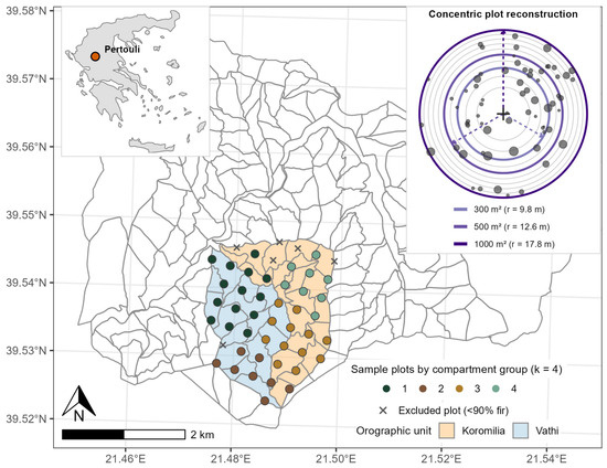
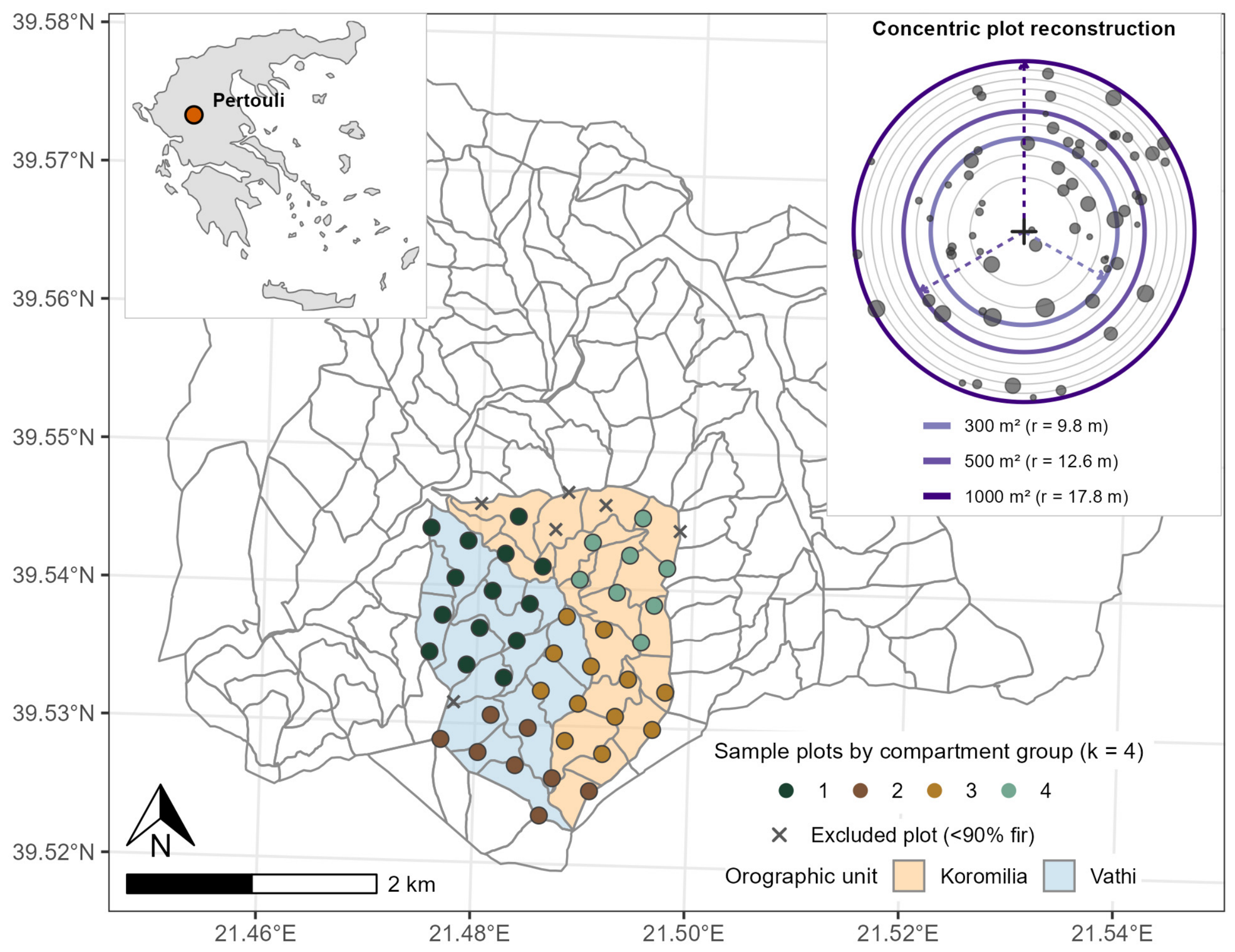
We estimated tree density (, stems ha−1) and basal area (BA, m2 ha−1). Single-tree basal area was , where is DBH in cm [22]. Tree height was available only for a small opportunistic subset, and growing-stock volume was, therefore, outside the scope of the study. Figure 1 shows the study area, systematic sampling grid, fir-domain classification of the sample plots, and concentric-plot reconstruction.
Figure 1.
University Forest of Pertouli, central Greece, showing forest compartments, the 42 fir-domain sample plots grouped by the four spatial compartment groups, and the six excluded plots with <90% fir. The upper-left inset locates Pertouli within Greece; the upper-right inset illustrates concentric reconstruction within a representative stem-mapped 1000 m2 plot, with 300, 500, and 1000 m2 plot sizes highlighted.
2.2. Concentric Plot Reconstruction and Full-Sample Estimators
Each 1000 m2 stem-mapped plot was reconstructed concentrically at m2. The corresponding circular radius was
A tree was included at area when its mapped distance from the plot center was not greater than . The per-hectare value for attribute on plot was obtained by expanding the total inside the reconstructed circle:
where for tree density and for basal area.
At each plot size, the full-sample mean, between-plot standard deviation, standard error, coefficient of variation, and relative standard error were
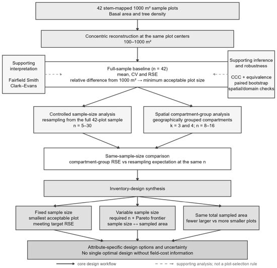
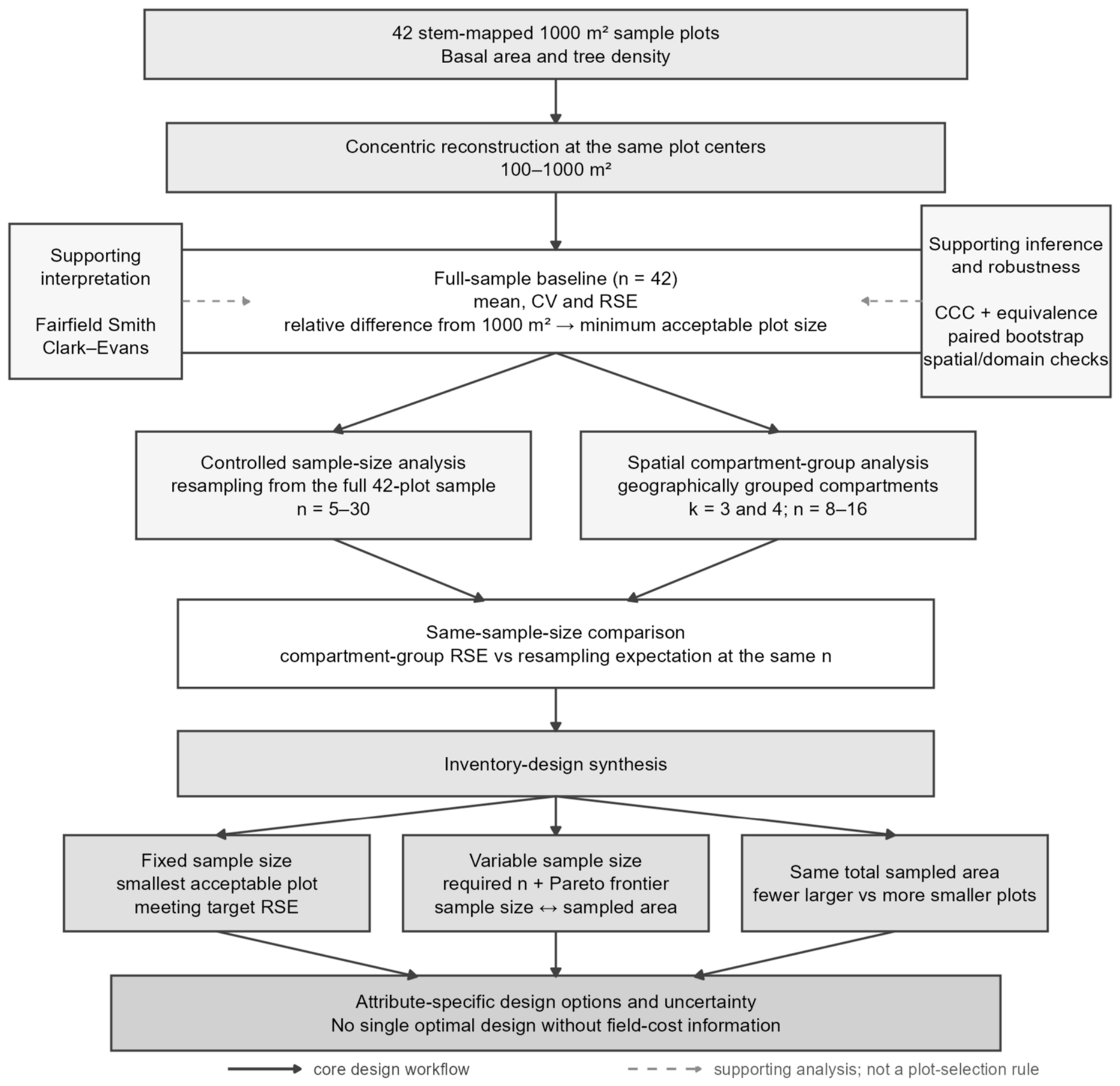
Here, for the full-sample analysis. The randomized-start systematic grid provides equal inclusion probabilities for the mean. Because only one realization of the systematic grid is available, variance and RSE were calculated using the simple-random-sampling (SRS) variance as a working approximation, following common forest-inventory practice [22,23]. The relationship between the SRS approximation and the variance of a systematic forest sample depends on between-plot spatial structure and on the variance estimator used; we therefore refer to the 42 plots as the full sample, not as a statistical population, and qualify variance-based inference with spatial diagnostics (Section 2.7). The core design workflow and the distinction between design-driving and supporting analyses are summarized in Figure 2.
Figure 2.
Core plot- and sample-size design workflow and supporting analyses. Solid arrows show the analyses used directly to evaluate inventory designs. Controlled sample-size resampling and spatial compartment-group analysis are compared at the same sample size before fixed-sample-size, variable-sample-size/Pareto, and same-total-sampled-area design options are evaluated. Dashed boxes identify supporting analyses used for structural interpretation, inference, and robustness rather than plot-size selection.
2.3. Agreement with the 1000 m2 Reference and Full-Sample Precision
The 1000 m2 reconstruction was treated as the measured reference at each plot center. For each smaller plot size, we calculated the relative difference in the full-sample mean,
This is a reference difference, not estimator bias: smaller and larger plots are nested measurements at the same centers, and the 1000 m2 value is itself an estimate.
For operational comparison, we adopted a ±10% practical agreement criterion on . This criterion concerns the relative difference in the full-sample mean and is not an RSE threshold or a universal equivalence standard. To avoid selecting an isolated small plot that passes only because of non-monotonic local variation, the minimum acceptable plot size was defined as the smallest tested area from which that area and every larger tested area remained within the criterion. Sensitivity was evaluated under ±7.5% and ±5% agreement criteria.
Plot-level agreement was summarized by Lin’s concordance correlation coefficient (CCC) [24],
where and denote the paired vectors of plot-level values at area and at the 1000 m2 reference, respectively. The coefficient measures agreement about the 1:1 line by accounting for both association and departures in location and scale. No CCC cutoff was used for plot-size selection.
Formal equivalence of the paired mean difference was assessed secondarily with two one-sided tests (TOST) [25] at and a ±10% equivalence margin relative to the 1000 m2 mean. Equivalence required both one-sided tests to reject, which is equivalent to the 90% confidence interval for the paired difference lying wholly within the margin. A distribution-free companion resampled whole plot identities with replacement () and declared equivalence when the 90% percentile-bootstrap interval for the relative difference lay wholly within ±10%. For plot sizes that failed TOST while their observed relative difference remained inside the margin, a sensitivity calculation held the observed paired mean difference and dispersion fixed and increased until the TOST criterion was met. These projected sample sizes quantify the sample-size dependence of formal equivalence; they are not predictions for a future denser grid. Because the equivalence procedures treat plot units as exchangeable under the SRS working approximation, their thresholds are reported as conditional results.
Precision comparisons with the 1000 m2 design used a paired plot-level bootstrap (). Whole plot identities were resampled, and the RSE at the candidate size and 1000 m2 was recomputed on the same resample. The RSE ratio and the RSE difference were summarized by 95% percentile intervals. This paired analysis avoids judging a difference from overlap of separate marginal confidence intervals.
2.4. Sample-Size Requirements, Pareto-Efficient Designs, and Joint-Attribute Designs
For a target RSE expressed in percent, the sample size implied by the observed coefficient of variation is
Here, denotes rounding upward to the next integer, and is the projected total sampled area. No normal or quantile enters Equation (7) because the target is the relative standard error itself, not a confidence-interval half-width. Uncertainty in arises instead from estimating from 42 plots and from projecting the observed variance structure to a different spatial sample. We propagated CV uncertainty by whole-plot bootstrap ().
We evaluated 5% and 10% RSE scenarios. Any design requiring is explicitly a projection beyond the observed sample because additional plots would imply a denser grid and inter-plot distances not represented in the present data. For interpretation of these projections, the approximate spacing of an equivalent square grid was calculated as , where is the estimated fir-domain area in hectares. The existing sample is shown as an operational reference, not as a Pareto constraint.
Among plot sizes at or above the minimum acceptable plot size, a design was classified as Pareto-efficient (non-dominated) for a given target when no alternative design required both (i) no more sample plots and (ii) no more total sampled area, with at least one quantity strictly smaller. The Pareto frontier is the set of these non-dominated designs. Multi-objective forest-inventory optimization has similarly used Pareto-efficient sets when cost and variance are competing design objectives [26]. In the present analysis, sample size and total sampled area are the two explicit design objectives; monetary cost is not optimized because a complete field-cost model was not measured. The frontier therefore displays the observed design trade-off without assigning monetary weights to plot establishment, travel, or within-plot measurement; the final choice along the frontier depends on management priorities and per-plot costs.
Because basal area and tree density are measured on the same sample plots, we also evaluated joint precision scenarios. For each plot size,
where and are the attribute-specific required sample sizes. We evaluated three target combinations: BA 10%/N 10%, BA 5%/N 10%, and BA 5%/N 5%.
2.5. Controlled Sample-Size Reduction and Spatially Grouped Forest Compartments
The sample-size analysis comprised three linked analytical components. First, the full-sample baseline used all 42 plots to quantify plot-size agreement and precision at the observed study-area scale. Second, the controlled sample-size analysis resampled those 42 plots at smaller sample sizes (–30) to isolate the plot-size × sample-size precision response. Third, the spatial compartment-group analysis calculated RSE within geographically grouped forest compartments containing 8–16 observed plots, thereby retaining the spatial coherence of smaller forest-management units. The latter two components were compared at the same sample size.
To quantify the effect of sample size independently of a specific geographic subdivision, plots were resampled with replacement from the full 42-plot sample. For every integer and every reconstructed plot size, 2000 resamples were used to obtain the median RSE and its 2.5th and 97.5th percentiles. Representative 300, 500, and 1000 m2 results are shown in the main figure. This procedure describes the precision expected from resampling the observed 42 plots at a given ; it does not represent an observed denser systematic grid.
A complementary analysis retained geography. The sampled forest compartments were grouped from their centroid coordinates using partitioning around medoids (PAM) [27]. Aggregation of forest management units through clustering has been proposed as a way to improve the reliability of direct estimates [28]. In the present study, however, clustering was deliberately based only on standardized geographic centroid coordinates: easting and northing were standardized before clustering, and no forest attribute or remote-sensing variable entered the grouping. We examined and as two grouping granularities that produced geographically compact groups containing approximately 8–16 observed plots. Plots inherited the group assigned to their compartment. The observed compartment-group sample sizes were 16, 13, and 13 plots for , and 14, 8, 12, and 8 plots for . Tree-density and basal-area means, standard deviations, standard errors, CVs, and RSEs were recalculated for every plot size within each compartment group.
To separate the influence of sample size from geographic grouping, each compartment-group RSE was compared with the resampling distribution for the same attribute, plot size, and sample size (the same-sample-size benchmark). We recorded whether the observed compartment-group RSE fell within the corresponding 95% resampling interval and the ratio of the observed RSE to the resampling median. Controlled resampling varies while averaging across the full sample; the compartment-group analysis retains geography and also reflects local forest heterogeneity. Similarity between the two indicates how much of the observed compartment-group precision can be explained by sample size, while geographic differences and local heterogeneity remain possible influences.
2.6. Same-Total-Sampled-Area Comparison Within the Observed 42 Plots
We tested the same-total-sampled-area question empirically using only the observed sample plots. Equal-area pairs were 1000 → 500, 800 → 400, and 600 → 300 m2. For each pair, a larger-plot sample of , 15, or 20 was compared with a smaller-plot sample of , 30, or 40, so total sampled area was exactly equal. For a fixed forest area, equal total sampled area also means equal areal sampling intensity (the percentage of forest area sampled), although the number and spatial density of sample plots differ. In each of 5000 replicates, plot identities were sampled without replacement from the observed 42-plot pool; of those identities were then sampled without replacement for the larger-plot design. The larger-plot sample was therefore nested within the smaller-plot sample, mimicking a design in which the original locations are retained at the smaller area and the saved sampled area is used to include additional observed locations.
The primary statistic was
Values below 1 favor the smaller/more-numerous design. We report the median ratio, its 95% resampling interval, and the percentage of scenarios in which the smaller/more-numerous design had lower RSE. This percentage is a descriptive resampling frequency, not a value.
2.7. Supporting Structural and Robustness Analyses
The core design analyses comprised concentric reconstruction, design-based estimation, the plot-size agreement criterion, RSE-based sample-size requirements, the sample-size/compartment-group comparison, Pareto evaluation, and the same-total-sampled-area comparison. CCC and equivalence tests were used as secondary inferential checks of agreement; Fairfield Smith and Clark–Evans provided structural interpretation; and the remaining analyses assessed robustness.
The between-plot variance response was summarized by the Fairfield Smith variance–plot-area relationship [5],
where is the scale constant and is the variance–plot-area exponent. The relationship was fitted by ordinary least squares to versus , so the fitted slope is . Whole-plot bootstrap intervals () accounted for dependence among the ten concentric reconstructions. Basal area and tree density were refitted on the same bootstrap resamples to obtain a paired interval for the difference between their exponents. Within-plot stem pattern was assessed independently with the Donnelly edge-corrected Clark–Evans nearest-neighbor index [29,30]. For a plot containing trees, the observed mean nearest-neighbor distance was divided by the edge-corrected expectation under complete spatial randomness; values below 1 indicate clustering, 1 indicates randomness, and values above 1 indicate regularity. The mean index was compared with 1 using a one-sample test, with a Wilcoxon signed-rank test as a distribution-free companion. At the 1000 m2 reference size, the association between basal area and tree density across plots was summarized by Pearson correlation with a 95% confidence interval and by Spearman correlation as a rank-based companion.
Additional checks addressed mean stability, the fir-domain definition, finite-population effects, equivalence multiplicity, alternative measures of variable measurement effort, the local 200 m2 radial anomaly, and between-plot spatial dependence. Plot-size effects on the mean were assessed with the Friedman test and a repeated-measures mixed model with a random plot intercept and a first-order autoregressive within-plot correlation structure over the ordered concentric sizes [31]. Spatial diagnostics used permutation Moran’s [32], distance-band sensitivity, and a spatial block bootstrap that resampled compact groups of plot centers. These analyses qualify the main results rather than define the selected plot size. Additional methodological details are provided in Appendix B.
2.8. Software and Reproducibility
Analyses were performed in R 4.4.3 with a fixed random seed of 42. Data handling and graphics used tidyverse 2.0.0 and ggplot2 4.0.2. Mixed-effects analyses used nlme 3.1-167 and analyses used spdep 1.4-2 and sf 1.0-21, and PAM clustering used cluster 2.1.8. Data import and project paths used readxl 1.4.5 and here 1.0.1. Figure production additionally used patchwork 1.3.1 and ggrepel 0.9.6. Figure 1 used ggspatial 1.1.9 for cartographic elements and maps 3.4.3 for the Greece locator.
3. Results
lme4 1.1-36; spatial compartment grouping used cluster 2.1.8; and between-plot spatial.
Results are presented first for the full 42-plot sample and then for reduced sample sizes and spatial compartment groups. The final analyses compare plot-size/sample-size trade-offs, same-total-sampled-area designs, and supporting robustness checks.
3.1. Full-Sample Agreement and Precision Across Plot Size
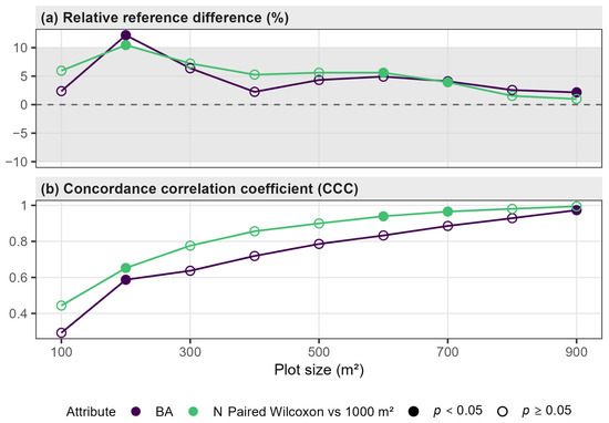
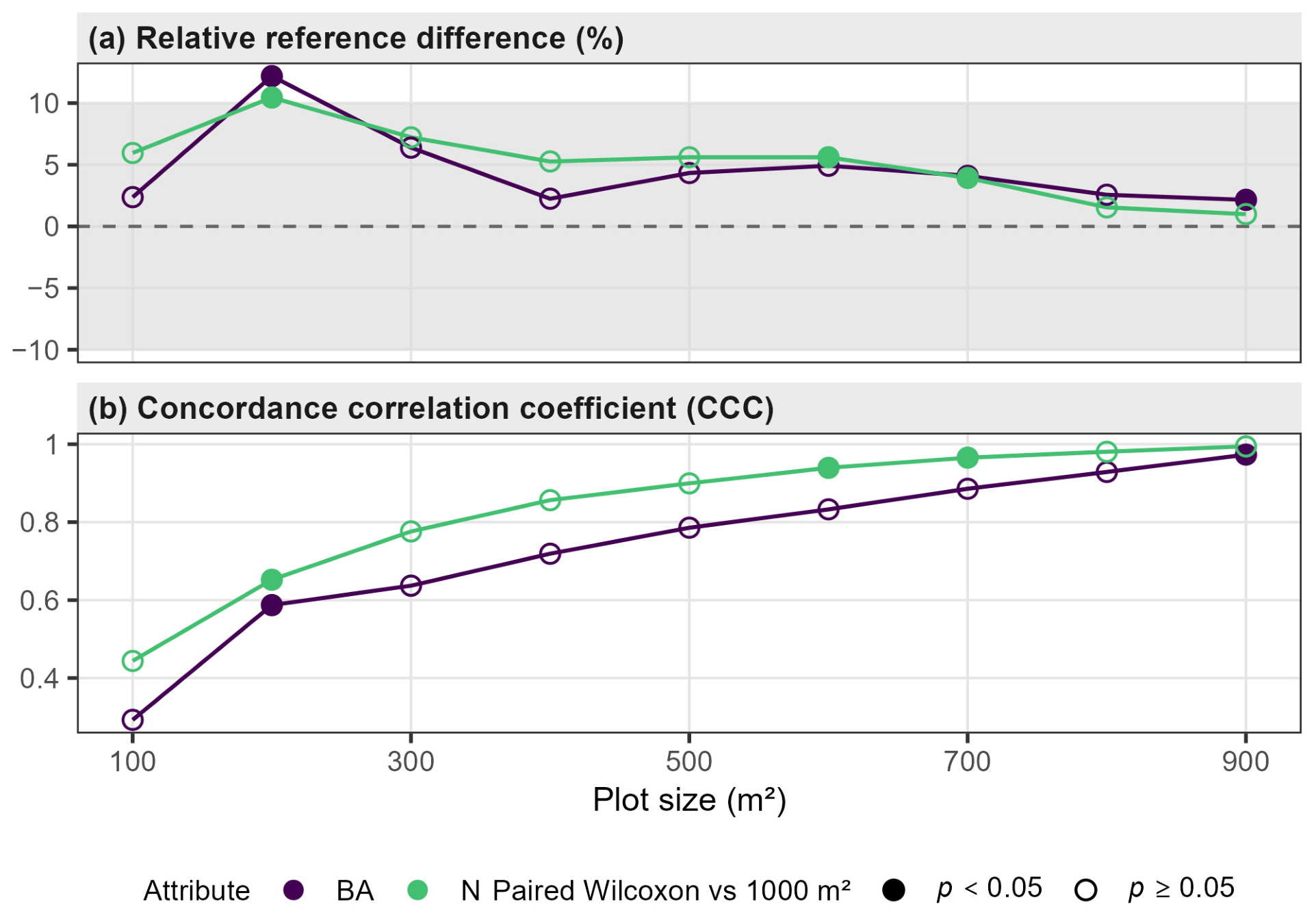
At the 1000 m2 reference size, mean basal area was 31.45 m2 ha−1 (CV 27.1%, RSE 4.18%) and mean tree density was 687.6 stems ha−1 (CV 38.2%, RSE 5.89%). Mean estimates across reconstructed sizes were broadly stable, but the 200 m2 reconstruction showed a clear local increase: relative to 1000 m2, basal area was +12.2% and tree density +10.5%. At 300 m2 the corresponding differences were +6.4% and +7.2%, and all sizes from 300 to 900 m2 were within ±10% for both attributes.
Under the continuous agreement rule, 300 m2 was the minimum acceptable plot size for both attributes (Figure 3). The isolated 100 m2 reconstruction also fell within the ±10% agreement criterion (BA +2.4%, N +6.0%), but the 200 m2 reconstruction did not, so 100 m2 could not begin a continuous acceptable sequence. Tightening the agreement criterion from ±10% to ±7.5% did not change the 300 m2 minimum. Under the ±5% agreement criterion, the minimum increased to 400 m2 for basal area and 700 m2 for tree density.
Figure 3.
Relative difference of the full-sample mean from the 1000 m2 reference and Lin’s concordance correlation coefficient (CCC) across reconstructed plot sizes. The shaded band shows the adopted ±10% practical agreement criterion, and the dashed horizontal line indicates zero relative difference from the 1000 m2 reference. CCC is descriptive and is not used as a pass/fail criterion.
Formal equivalence was more conservative and sample-size dependent. At , paired TOST and percentile-bootstrap equivalence with a ±10% equivalence margin both began at 400 m2 for basal area and 600 m2 for tree density. The failure at 300 m2 was principally a power limitation: the TOST calculation indicated that approximately 156 plots for basal area and 292 for tree density would be needed to certify the observed 300 m2 differences at that margin, whereas the 200 m2 difference itself exceeded the margin. Because equivalence inference inherits the between-plot exchangeability assumption, these thresholds are reported as secondary inferential results rather than as the operational selection rule.
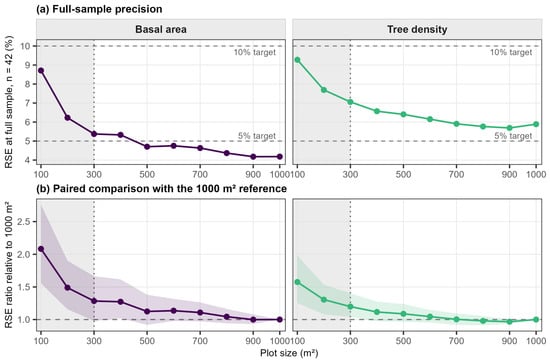
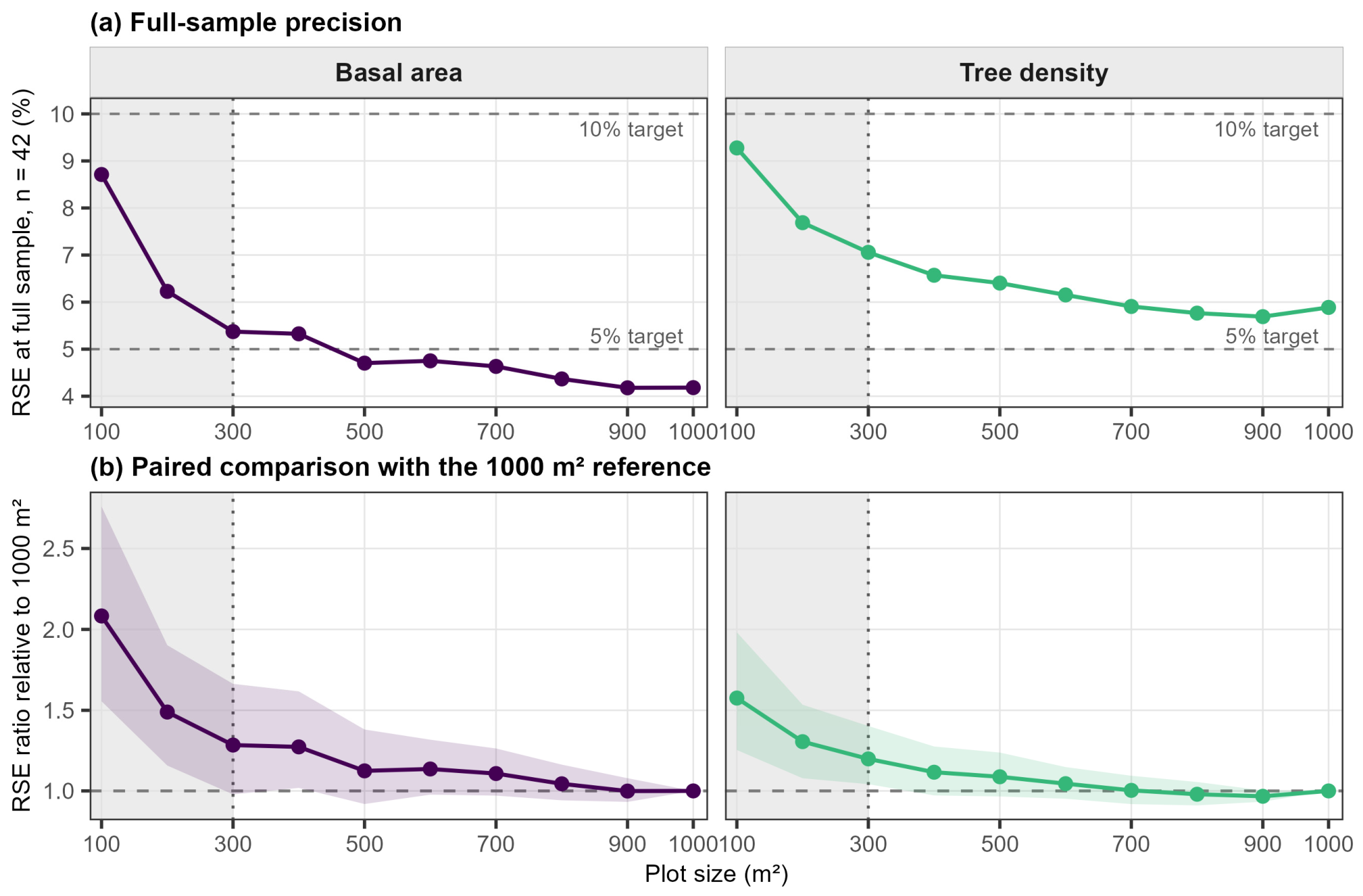
Full-sample RSE increased as plot area decreased, but not monotonically at every 100 m2 step (Figure 4a). At the observed , basal-area RSE was 4.18% at 1000 m2 and remained at or below 5% continuously from 500 m2 upward; at 300 and 400 m2 it was 5.37% and 5.33%, respectively. Tree density was less precise: its lowest observed RSE was 5.69% at 900 m2, and no reconstructed plot size met the 5% RSE target with the existing 42 plots. Both attributes remained below 10% throughout the 300–1000 m2 acceptable range.
Figure 4.
Precision across reconstructed plot sizes in the full 42-plot sample. (a) RSE across plot sizes; horizontal dashed lines mark 5% and 10% RSE targets. (b) Paired bootstrap ratio of RSE at each reconstructed plot size to the RSE of the 1000 m2 reference. Lines connect the plot-size-specific RSE-ratio estimates, and shaded ribbons show the corresponding 95% bootstrap percentile intervals. A ratio of 1 indicates equal precision; ratios above 1 indicate higher RSE and lower precision than the 1000 m2 reference. In both panels, the vertical dotted line marks the 300 m2 minimum acceptable plot size, and the shaded region identifies the 100–200 m2 sizes below that minimum.
The paired bootstrap comparison with 1000 m2 then quantified whether these precision differences were distinguishable while preserving the common plot centers (Figure 4b). For basal area, the RSE ratio at 500 m2 was 1.12 (95% interval 0.92–1.38); at 400 m2 it was 1.27 (1.02–1.62), whereas the 300 m2 ratio of 1.28 had a wider interval (0.98–1.66). For tree density, the 300 m2 ratio was 1.20 (1.04–1.40), while ratios from 400 to 900 m2 had intervals including 1. The non-monotonic inferential result at 300 versus 400 m2 for basal area reflects bootstrap uncertainty and should not be read as evidence that 300 m2 is intrinsically more stable than 400 m2.
Taken together, the full-sample results identify 300 m2 as the minimum acceptable plot size under the ±10% practical agreement criterion. At , basal area attained the 5% RSE target from 500 m2, whereas tree density did not attain 5% RSE at any acceptable plot size. Both attributes attained the 10% RSE target from 300 m2. These full-sample design implications are summarized in Table 1.
Table 1.
Full-sample design interpretation at the observed .
3.2. Sample-Size Response from the Full 42-Plot Sample
Reducing sample size caused a much larger increase in RSE than the differences among moderate plot sizes. At , mean bootstrap RSE was 11.3%, 12.7%, and 14.3% for basal area at 1000, 500, and 300 m2, respectively; corresponding tree-density values were 15.7%, 17.3%, and 18.8%. In the discrete sample-size scenarios, mean bootstrap RSE fell below 10% for basal area at approximately , 10, and 15 for 1000, 500, and 300 m2, respectively; the corresponding tree-density sample sizes were approximately , 20, and 20. The 15% RSE reference level was attained at smaller sample sizes, especially for basal area.
These results show that achievable precision depends strongly on sample size. A 5% RSE target can be realistic for the full 42-plot sample but is generally too demanding for compartment groups containing only 8–16 plots. Accordingly, the sample-size/compartment-group figure uses 10% and 15% RSE as visual reference levels, while the full-sample Pareto analysis below uses 5% and 10% RSE targets.
3.3. Precision Within Spatially Grouped Forest Compartments
The spatial partitions produced three groups with 16, 13, and 13 plots, and four groups with 14, 8, 12, and 8 plots. RSEs calculated within these compartment groups varied substantially, as expected from the small sample sizes. For example, at 1000 m2 the four-group basal-area RSEs were 6.0%, 8.6%, 7.9%, and 10.9%.
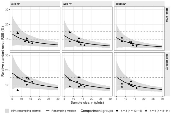
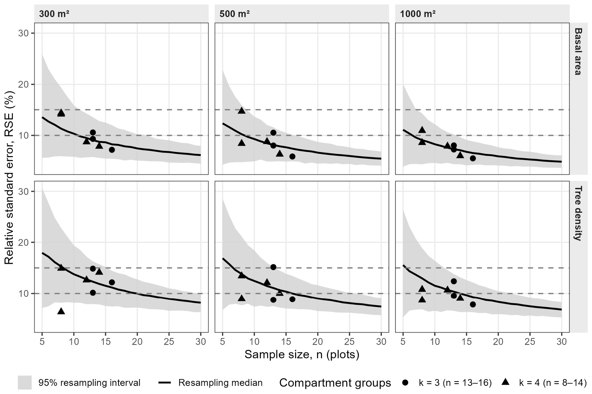
The compartment-group RSEs were compared with the resampling expectation at the same sample size. They did not show a systematic additional precision penalty (Figure 5). Across all ten reconstructed plot sizes, 100% of basal-area group-by-size comparisons fell inside the corresponding 95% resampling interval for both and . For tree density, 96.7% did so for and 95.0% for . Median ratios of compartment-group RSE to the resampling median at the same sample size were 1.00 and 0.96 for basal area and 0.92 and 0.95 for tree density under and , respectively.
Figure 5.
Sample-size response and precision within spatially grouped forest compartments. Black curves and gray bands show the median and 95% interval from resampling the full 42-plot sample for each sample size. Points are RSE values calculated within geographically compact compartment groups (: –16; : –14). Horizontal lines at 10% and 15% RSE provide reference levels appropriate to these smaller samples. Columns show 300, 500, and 1000 m2 for readability; the same-sample-size comparison was evaluated across all ten plot sizes.
The close agreement indicates that the loss of precision within compartment groups is largely consistent with their smaller sample sizes. Geography and local forest structure may still contribute because the compartment groups are fixed local domains, whereas the resampling curves average over repeated samples from the full observed 42-plot sample.
3.4. Pareto-Efficient Plot-Size and Sample-Size Designs
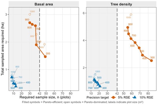
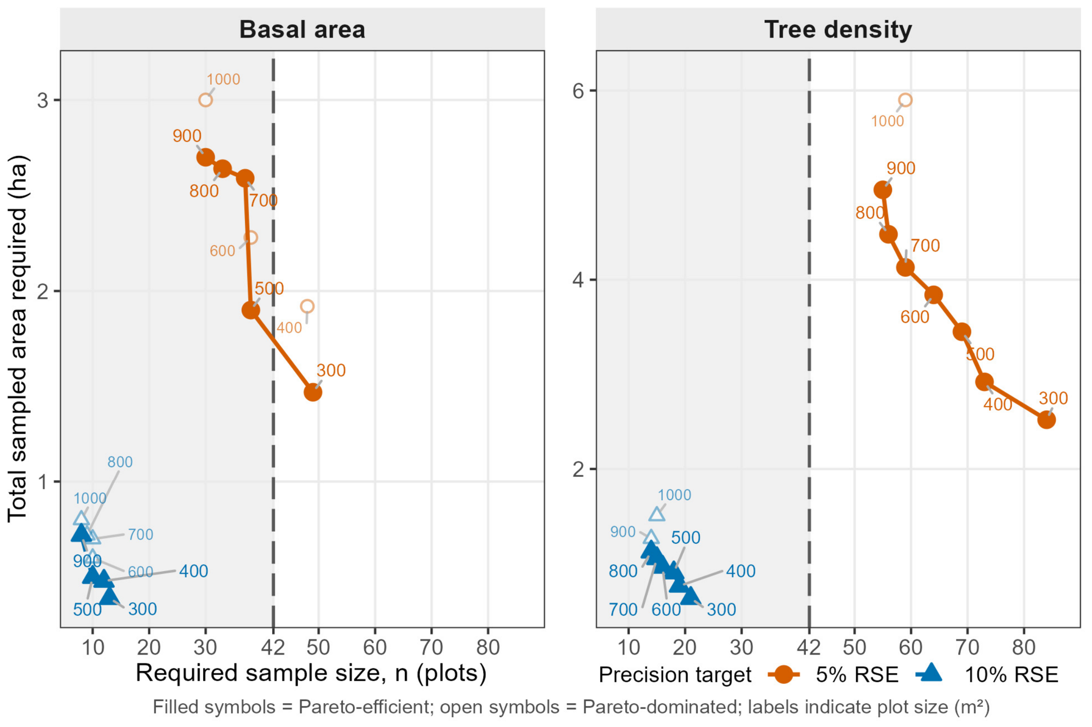
The sample-size projections made the difference between basal area and tree density explicit (Figure 6). For a 5% RSE target, the basal-area Pareto frontier included 300 m2/ (1.47 ha sampled), 500 m2/ (1.90 ha), 700 m2/ (2.59 ha), 800 m2/ (2.64 ha), and 900 m2/ (2.70 ha). The 400, 600, and 1000 m2 alternatives were dominated because another plot size required both no more plots and no more sampled area. The 300 m2 design minimized sampled area, while larger frontier designs progressively reduced sample size.
Figure 6.
Required sample size and total sampled area for candidate plot sizes of 300–1000 m2 under 5% and 10% RSE targets. Circles represent the 5% RSE target and triangles the 10% RSE target. Filled symbols denote Pareto-efficient designs, whereas lighter open symbols denote Pareto-dominated evaluated designs. Numeric labels identify Pareto-efficient plot sizes (m2); the 1000 m2 reference is also labeled when dominated. Solid and dashed lines connect successive Pareto-efficient designs for the 5% and 10% RSE targets, respectively, for visual guidance. The vertical dashed line denotes the observed sample size (), and the shaded region identifies designs whose required sample size does not exceed 42 plots. Required sample sizes are projections from the observed CVs; designs with imply denser spatial sampling than was observed.
The observed sample provides the practical reference for feasibility. At 5% RSE, the 300 m2 basal-area design would require a projected 49 plots, whereas 500 m2 requires 38; thus 500 m2 is the smallest acceptable Pareto-efficient basal-area design whose projected requirement does not exceed the existing sample size. Tree density differed sharply: every 5% Pareto-efficient design required more than 42 plots, ranging from 84 plots at 300 m2 to 55 at 900 m2. The 5% density target is therefore not achievable within the current sample under the observed variance estimates.
At a 10% RSE target, both attributes were feasible within . The Pareto frontier began at 300 m2/ for basal area and 300 m2/ for tree density. Results differed between the 5% and 10% RSE targets, showing that design adequacy depends on both the attribute and the precision target.
Joint-attribute designs showed the same attribute dependence (Table 2). When both basal area and tree density were assigned 10% targets, the minimum-sampled-area design was 300 m2 with , limited by tree density. For BA 5%/N 10%, 300 m2 minimized sampled area but required 49 plots, whereas 500 m2 required 38 and was therefore feasible within the existing 42-plot sample. When both attributes were assigned 5% targets, tree density controlled the design at every plot size and the minimum-sampled-area scenario was 300 m2 with 84 plots.
Table 2.
Joint basal-area/tree-density precision scenarios.
3.5. Same Total Sampled Area: Fewer Large Plots Versus More Small Plots
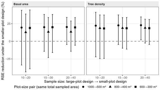
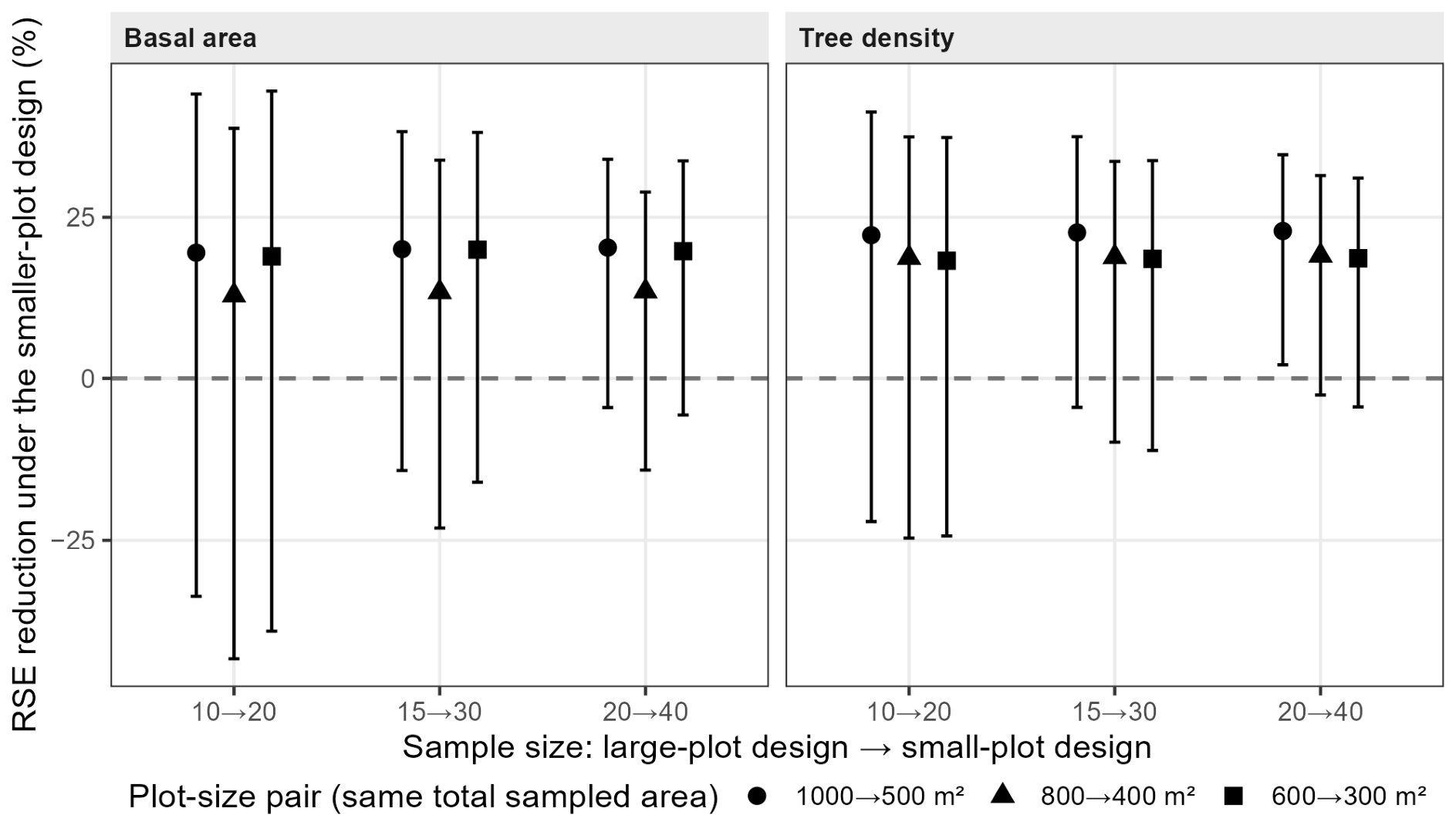
The same-total-sampled-area analysis used only the observed 42 sample plots, avoiding any claim that a denser future systematic grid had been empirically observed. In all 18 attribute × plot-size-pair × sample-size scenarios, the median RSE ratio was below 1: measuring the same total sampled area with a larger number of smaller plots reduced the median RSE.
For basal area, median ratios ranged from 0.797 to 0.872, corresponding to median RSE reductions of approximately 13%–20%. The smaller/more-numerous design had lower RSE in 72.9%–95.1% of resamples. For tree density, median ratios ranged from 0.771 to 0.817, or reductions of approximately 18%–23%, and the smaller/more-numerous design had lower RSE in 83.7%–98.1% of resamples. The directional result strengthened as sample size increased.
The clearest individual comparison was 20 × 1000 m2 versus 40 × 500 m2. Median RSE ratios were 0.797 for basal area and 0.771 for tree density; the smaller-plot design was more precise in 95.1% and 98.1% of resamples, respectively. Only the tree-density interval for this comparison was entirely below 1 (95% interval 0.653–0.979). The percentages are descriptive resampling frequencies, not significance probabilities. The RSE reductions for all equal-area comparisons are summarized in Figure 7.
Figure 7.
Effect of distributing the same total sampled area among more small plots rather than fewer large plots. For a fixed forest area, the paired designs have the same areal sampling intensity. Each comparison halves plot area and doubles sample size (1000→500, 800→400, and 600→ 300 m2). Points show the median percentage reduction in RSE across resamples drawn only from the 42 observed plots; vertical bars show 95% resampling intervals. The horizontal dashed line marks zero change in RSE. Positive values indicate greater precision for the smaller-plot design.
3.6. Supporting Structural and Robustness Results
The variance–plot-area relationship was strong for both attributes (Appendix A Figure A1): for basal area (, bootstrap 95% interval 0.384–0.881) and for tree density (, 0.266–0.684). However, the paired bootstrap difference had a 95% interval of −0.139 to 0.467, so the exponents were not statistically distinguishable. Attribute differences in the design analysis should therefore be interpreted from the observed CV/RSE response rather than from the ordering of the fitted exponents.
The Clark–Evans index confirmed clustered within-plot stem pattern (mean 0.878, 95% CI 0.845–0.910; one-sample test ; Appendix A Figure A2). At 1000 m2, basal area and tree density were only moderately correlated across plots (Pearson , 95% CI 0.032–0.578; ), supporting their treatment as separate precision targets.
Between-plot spatial diagnostics did not detect significant autocorrelation at the measured 316 m grid lag: across plot sizes the largest absolute Moran’s was 0.159 and the smallest permutation value was 0.064. This is not evidence of independence. Spatial block resampling produced attribute- and plot-size-specific effects on interval width: relative to independent resampling, width ratios at 1000/500/300 m2 were 0.79/0.81/0.93 for basal area and 1.01/1.32/1.34 for tree density. Density uncertainty at smaller plots is therefore more sensitive to spatial resampling, and formal equivalence and required-sample-size results remain conditional on the SRS variance approximation.
The all-48-plot domain estimator provided a separate check on the 42-plot domain analysis. At 300, 500, and 1000 m2, domain-estimator means were identical to the corresponding 42-plot fir-domain means and RSEs differed by only about 0.01 percentage points because the two estimators are algebraically very similar in this setting. Excluding the single borderline fir plot reduced the full sample to 41 plots but left the 300 m2 acceptable-range limit and the main variance response essentially unchanged; adding the six mixed plots would change the target forest domain and was therefore not treated as a sensitivity test.
Additional sensitivity analyses gave the same ordering of the principal design choices. At the 1.13% sampled-area intensity, a finite-population correction changed none of the projected required sample sizes. Correcting the formal-equivalence tests for multiple plot-size comparisons moved the equivalence limits upward (to 700 m2 for both attributes under a nine-comparison correction, and to 800 m2 for basal area and 700 m2 for tree density under an 18-comparison correction). These stricter limits further distinguish formal equivalence from the practical agreement criterion. At the 5% RSE target, the same plot size minimized both the expected number of measured trees and total sampled area; neither measure includes fixed travel or plot-establishment cost.
Finally, uncertainty in the required sample sizes was substantial. At 5% RSE, for example, basal area required 49 plots at 300 m2 with a bootstrap interval of 28–71 and 38 at 500 m2 with 23–53; tree density required 84 at 300 m2 with 53–112 and 69 at 500 m2 with 44–96. These intervals quantify uncertainty in the observed CV. They do not address the additional change in spatial covariance that could occur when a future systematic grid is made denser.
4. Discussion
The results identify a design trade-off rather than a single optimal plot size. Its practical interpretation depends on the agreement criterion, target attribute and RSE, available sample size, and the distribution of sampled area among plots.
4.1. Plot Size Is Not a Single-Criterion Decision
No single plot size satisfied all design criteria. The data do not identify a universal “best” plot size or a formal 300–500 m2 optimum. Instead, they identify a minimum acceptable plot size followed by trade-offs among sample size, sampled area, attribute, and precision target.
The minimum acceptable plot size is 300 m2 under the adopted ±10% practical agreement criterion for the full-sample mean. The result is stable under a moderate tightening of the criterion: ±7.5% gives the same minimum for both attributes, whereas ±5% gives 400 m2 for basal area and 700 m2 for tree density. The ±10% criterion is a practical case-study threshold rather than an external equivalence standard.
The formal-equivalence analysis addresses a different question from the practical agreement criterion. It gave minimum sizes of 400 m2 for basal area and 600 m2 for tree density because uncertainty in the paired mean differences is included. These limits were treated as secondary inferential results; the 300 m2 minimum acceptable plot size should not be interpreted as evidence of formal equivalence.
The Pareto analysis addresses design choice after applying the plot-size agreement criterion. For basal area at a 5% RSE target, 300 m2 minimizes sampled area but requires 49 plots; 500 m2 requires 38 plots at a higher sampled area; and 900 m2 reduces the requirement further to 30 plots but samples substantially more area. None of these designs is universally optimal without knowing the relative field cost of establishing an additional plot versus measuring additional trees and area within a plot. Consistent with the multi-objective forest-inventory perspective of Angelis and Stamatellos [26], the frontier is therefore interpreted as a set of non-dominated design choices rather than as a single economic optimum.
4.2. Attribute and Precision Target Determine Feasibility
Basal area and tree density do not support a single common design conclusion. At the full sample of 42 plots, basal area already has an RSE of 4.18% at 1000 m2 and remains below 5% from 500 m2 upward. Tree density has a 1000 m2 RSE of 5.89%, so no change in plot size alone can make a 5% target feasible at the same 42 sample plots. In the 5% RSE Pareto analysis, basal area enters the region, whereas tree density does not.
At a 10% RSE target, both attributes are feasible from the 300 m2 minimum acceptable plot size. The appropriate design therefore depends on the precision target: 300 m2 is adequate at a 10% RSE target, whereas a 5% basal-area target favors at least 500 m2 if sample size is held to the existing 42 plots. A 5% tree-density target requires a larger sample, regardless of the acceptable plot size chosen.
The joint-attribute scenarios show why this distinction matters operationally. When both attributes are required at 10%, tree density controls the 300 m2 design at 21 plots. When basal area is tightened to 5% while density remains at 10%, basal area becomes limiting, and 500 m2 is the smallest acceptable size whose projected joint sample requirement fits inside 42 plots. When both targets are 5%, tree density again controls and the projected sample size rises well beyond the current inventory.
4.3. Sample Size Is the Main Constraint Within Compartment Groups
The compartment-group analysis links the full-sample results to estimation within smaller geographic groups of forest compartments. RSEs calculated within groups of 8–16 plots were substantially larger than full-sample RSEs, but 95%–100% of those observed values lay inside the corresponding resampling interval at the same sample size. This indicates that much of the precision deterioration is consistent with the reduction in sample size.
Spatial grouping may still affect precision because each compartment group occupies a specific part of the forest and may differ in site conditions or stand structure. The resampling curve mixes plots across the full fir domain, whereas the observed compartment-group RSEs retain those geographic differences. Their close correspondence provides a same-sample-size benchmark for interpreting the observed loss of precision. For this reason, Figure 5 uses 10% and 15% reference levels rather than the 5% target emphasized in the full-sample Pareto analysis. A group with only 8–16 plots cannot generally support the same precision target as the full 42-plot inventory. Plot-size selection for a group of forest compartments therefore cannot be separated from the sample size available within that group.
4.4. The Same Total Sampled Area Generally Gives Greater Precision When Distributed Among a Larger Number of Smaller Plots
Across all same-total-sampled-area scenarios based on the observed 42 plots, median RSE was lower when the same sampled area was distributed among a larger number of smaller plots. The median reduction was approximately 13%–20% for basal area and 18%–23% for tree density.
This result is consistent with the observed variance–plot-area relationship: variance declines with increasing plot area, but not rapidly enough for doubling plot area to compensate fully for halving the number of plots. Distributing the same sampled area among more plot centers represents spatial variability at more locations. The effect was stronger for tree density, although the uncertainty in the Fairfield Smith exponents did not support a statistically significant difference between attributes.
These precision gains do not necessarily imply lower field costs. Equal sampled area does not mean equal travel time, establishment time, perimeter work, or data handling. Earlier Pertouli sampling studies likewise showed that inventory efficiency depends on detailed field-time costs [33] and that walking cost can alter the optimum allocation in two-phase sampling [34]. Moving from 20 large plots to 40 smaller plots doubles the number of plot visits, and those fixed per-plot costs may offset or reverse the statistical gain. The result concerns precision at the same total sampled area; total inventory cost may differ because travel and plot-establishment costs were not measured.
4.5. Stand Structure Helps Explain Diminishing Returns
The supporting structural analyses are consistent with the observed design response. The Fairfield Smith variance–plot-area relationship [5] fitted the observed decline in between-plot variance closely ( for basal area and for tree density), with bootstrap estimates (95% CI 0.38–0.88) and (0.27–0.68), respectively. The paired bootstrap difference between the two exponents nevertheless included zero, so their ordering is treated descriptively rather than as evidence of different underlying laws. The accompanying Clark–Evans analysis showed clustered within-plot stem pattern. Together, these results support the interpretation that enlarging a plot incorporates additional nearby trees that are not spatially independent, so precision gains diminish as plot area increases. The Fairfield Smith relationship provides a structural interpretation of diminishing precision gains with increasing plot area; it is not used to select plot size.
Plot size also matters outside inventory estimation because, in growth-and-yield modeling, plot dimensions define the neighborhood over which competition is quantified. Hynynen and Ojansuu [35] found for Norway spruce that competition measures from plots averaging 116 m2 were dominated by sampling error and that increasing plot size increased model sensitivity to stand density and individual competitive status; their larger plot variant averaged 331 m2. Their objective differs from design-based inventory precision, so those plot sizes do not validate the 300–500 m2 case-study range found here, but the comparison reinforces that suitable plot dimensions are purpose-specific.
The local 200 m2 anomaly also appears to have a structural component. Comparing the inner 200 m2 disc with the 200–1000 m2 outer annulus across the same 42 plots showed approximately 15.7% greater basal area and 13.4% greater tree density in the inner disc, with paired Wilcoxon and 0.035. The second 100 m2 annulus—the area added when the 100 m2 plot becomes 200 m2—was the richest annulus for both attributes. Removing non-fir stems left the pattern essentially unchanged. The radial profile was nevertheless non-monotonic, explaining why 100 m2 happened to be closer to the 1000 m2 mean than 200 m2. The origin of the local concentration cannot be established from this study and may be site-specific; the pattern should not be interpreted as a general edge effect.
4.6. Limitations and Transferability
Several limitations define how far the design conclusions can be generalized.
First, all smaller plots are concentric reconstructions from the same 1000 m2 field plots. The 1000 m2 plot is a measured reference at each sampled center, not a census or a true population value; larger field plots or a wall-to-wall census could reveal additional spatial heterogeneity. The analysis estimates the effect of reducing area at the observed centers but does not validate an independent network of new 300 or 500 m2 plots at different centers. This shared-area dependence is a strength for paired comparison but a limitation for extrapolation. Reconstruction also requires accurate tree-to-center distances; the stem-mapped Field-Map coordinates were used for this purpose. Horizontal-distance measurement error can affect estimates from circular fixed-area plots, particularly at small radii and in relation to tree-position pattern [36].
Second, variance estimation uses the SRS working approximation for one randomized-start systematic-grid realization. Moran’s did not detect autocorrelation at the observed grid lag, but the density block-bootstrap results show that uncertainty can widen when spatial grouping is preserved. Formal equivalence and required-sample-size projections should therefore be read as conditional on the observed between-plot variance structure. Variance estimators developed specifically for systematic samples provide an alternative route: local-difference approaches have been evaluated for systematic forest inventories [23], and design-based local-density estimation provides another principled option [37]. We did not fit these alternatives here because the present analysis focuses on the plot-size comparison rather than a comparison of systematic-sample variance estimators.
Third, projected sample sizes above 42 imply a denser spatial grid. For the estimated 372.69 ha fir domain, for example, 49 plots correspond to an approximate spacing of 276 m and 84 plots to about 211 m, both shorter than the 316 m grid observed here. The present data cannot estimate covariance at those shorter distances. These projected sample sizes are design scenarios, not validated requirements for a future grid.
Fourth, the fir-domain area is estimated from the 42/48 share of sampled 1000 m2 plots. The resulting 372.69 ha should not be interpreted as a wall-to-wall mapped pure-fir polygon. It is an estimated extent under the plot-level fir-composition criterion and carries sampling uncertainty. The separate GIS area discrepancy (516.30 ha versus the management-plan area definitions) adds uncertainty to absolute area and sampling-intensity estimates.
Fifth, the study does not measure a complete field-cost model. Sample size and total sampled area are reported separately because field travel, plot establishment, within-plot movement, tree measurement, and data processing were not timed. A future field-cost study could identify an economic optimum along the Pareto frontier.
Finally, the study concerns one uneven-aged, effectively single-species fir forest and two core attributes. Growing-stock volume was excluded because the available height measurements did not constitute a designed stand-level height sample, so the double-entry (DBH + height) tariffs [16] could not be applied consistently. The remaining available single-entry (DBH-only) volume model [38] would make the resulting volume estimates largely a function of diameter and therefore strongly coupled to basal area; such estimates would not provide an independent assessment of how volume variance changes with plot area. Basal area is therefore informative about diameter-based stocking and is related to DBH-based volume prediction, but it is not a substitute for direct growing-stock-volume evaluation. Mixed stands, other forest structures, volume and biomass estimation, and independent plot networks require separate validation.
5. Conclusions
Concentric reconstruction of one stem-mapped inventory showed that plot size and sample size must be evaluated jointly. Under the adopted ±10% practical agreement criterion, 300 m2 was the minimum acceptable plot size for both basal area and tree density, but it was not a universal optimum. Formal equivalence was more conservative, beginning at 400 m2 for basal area and 600 m2 for tree density at , and was therefore retained as a secondary inferential check rather than as the rule defining the minimum acceptable size.
With the observed 42-plot sample, basal area met the 5% RSE target from 500 m2, whereas tree density did not meet the 5% RSE target at any acceptable plot size. At a 10% RSE target, both attributes were feasible from 300 m2. Pareto-efficient designs made the operational trade-off explicit: smaller plots reduced total sampled area, whereas larger plots reduced the required number of sample plots.
Within spatially grouped forest compartments, 95%–100% of the observed group-by-size RSE values fell within the corresponding same-sample-size resampling intervals, indicating that the lower precision of groups containing 8–16 plots was largely consistent with their smaller sample sizes. In the equal-area comparisons restricted to the observed 42-plot pool, distributing the same total sampled area among more, smaller plots reduced median RSE by approximately 13%–23%. Thus, within the evaluated design range, increasing the number of sampled locations can be more effective for precision than concentrating the same sampled area in fewer, larger plots.
The decision hierarchy is deliberately simple. Practical agreement with the measured reference defines the admissible plot-size range; RSE targets, required sample size, Pareto-efficient combinations, and equal-area comparisons then describe the design trade-offs within that range. CCC, formal equivalence, Fairfield Smith, Clark–Evans, and spatial/domain diagnostics provide agreement, structural, or robustness evidence but do not independently determine the selected plot size.
The main transferable result is therefore the procedure rather than the numerical case-study values. For a given forest, attribute, and precision target, the procedure is to define an acceptable plot-size range, evaluate sample-size and sampled-area trade-offs within that range, and distinguish results supported by the observed sample from projections requiring denser future sampling. The 300–500 m2 case-study values require independent validation before application to even-aged, single-layered, mixed-species, or other forest structures.
Author Contributions
Conceptualization, methodology, software, validation, formal analysis, investigation, data curation, writing—original draft preparation, and visualization, A.G.; project administration, resources, writing—review and editing, and supervision, M.J.D. All authors have read and agreed to the published version of the manuscript.
Funding
This research received no external funding.
Data Availability Statement
The R code/scripts and the raw field-plot data are available from the corresponding author on reasonable request.
Acknowledgments
We thank Georgios Stamatellos for providing the data as Scientific Project Manager (project code 72147). We also thank Petr Maděra, Faculty of Forestry and Wood Technology, Mendel University in Brno, Czech Republic, for the generous provision of the Field-Map instrument/system, which made the implementation of the project much more efficient. We further thank Panagiotis Chrysanthou, Forester–Environmentalist, for acting as intermediary and for his technical support with the Field-Map instrument/system. We also thank the three anonymous reviewers, whose comments prompted several additional analyses and sharpened the presentation.
Conflicts of Interest
The authors declare no conflict of interest.
Appendix A. Additional Tables and Figures
Table A1.
Notation.
Table A2.
Overall plot-size tests. Restricted to reconstructed sizes ≥ 300 m2, neither the Friedman test nor the repeated-measures mixed-model comparison with AR(1) within-plot correlation detected a plot-size effect on the mean for either attribute.
Table A3.
Full-sample estimates across reconstructed plot sizes ().
Table A4.
Structural baseline at the 1000 m2 reference scale. Quantiles are included because the uneven-aged diameter distribution is strongly non-normal. Panel (a) summarizes the 42-plot fir-domain analysis sample; panel (b) summarizes all 48 measured plots as a composition-sensitivity reference.
Table A5.
Agreement, formal equivalence, and projected sample size for 5% RSE. For the 1000 m2 reference, relative difference, concordance and equivalence against itself are not defined; only the projected sample size is reported.
Formal-equivalence limits are conditional on the exchangeability/SRS variance approximation. Multiplicity correction raises, rather than lowers, these limits; the uncorrected 400 m2 (BA) and 600 m2 (N) values are reported as secondary inferential results alongside the main agreement analysis.
Figure A1.
Fairfield Smith variance–plot-area relationship for basal area and tree density. The fitted exponents summarize the rate at which between-plot variance declines with plot area; their difference is not statistically distinguishable in the paired bootstrap. The relationship provides a structural interpretation of diminishing returns to plot enlargement and is not used to select plot size.
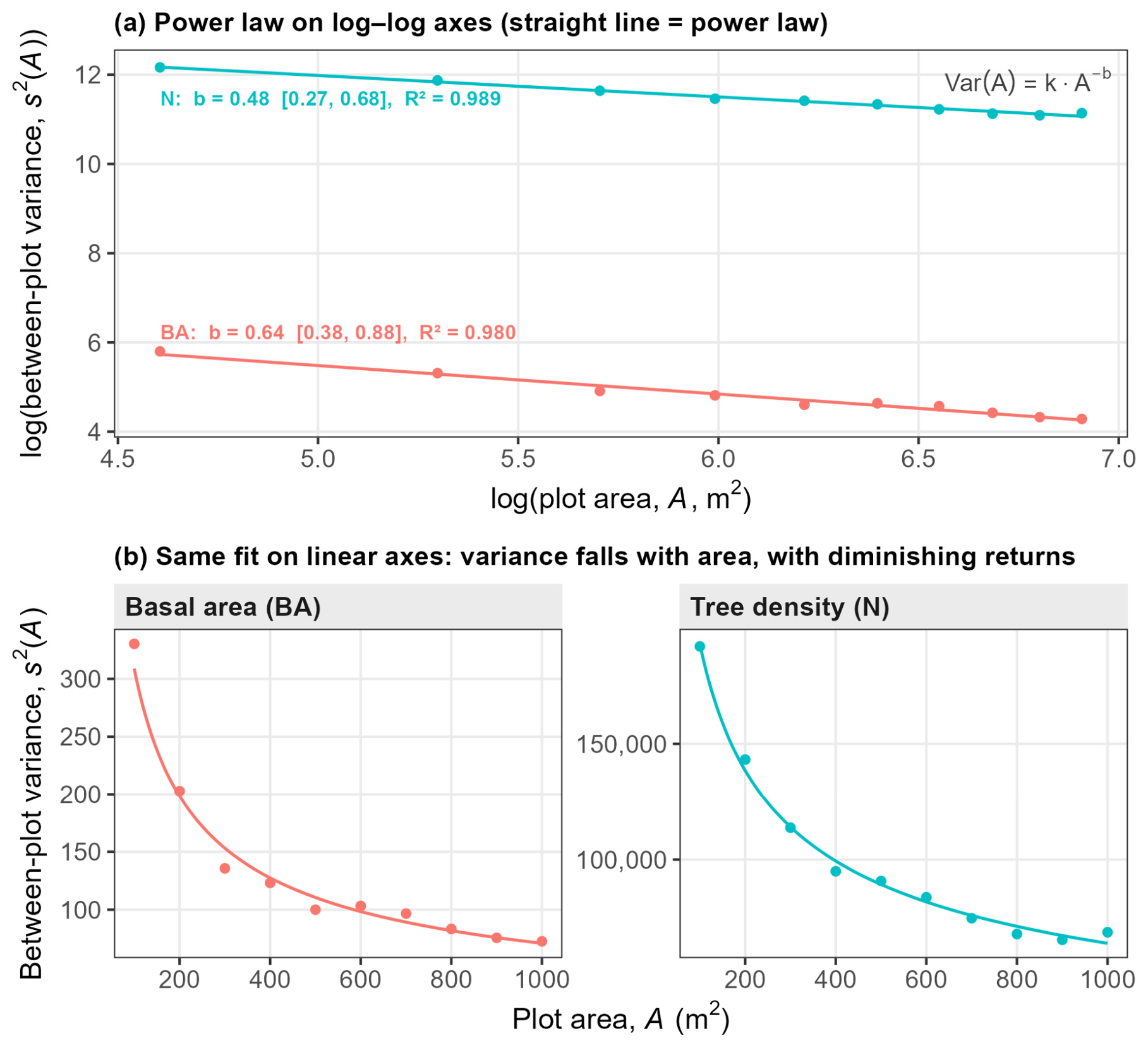
Figure A2.
Distribution of the Donnelly edge-corrected Clark–Evans index across the 42 sample plots. Values below 1 indicate clustered within-plot stem pattern.
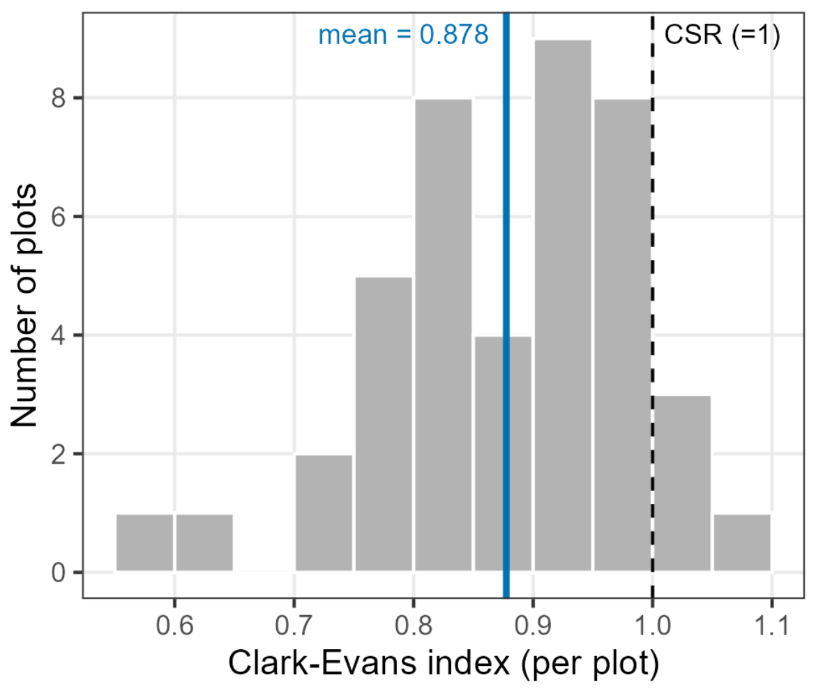
Figure A3.
Normal Q–Q plots of normalized residuals from the supporting repeated-measures mixed model. The distribution-free Friedman analysis is reported alongside the model because residual tails depart from normality.
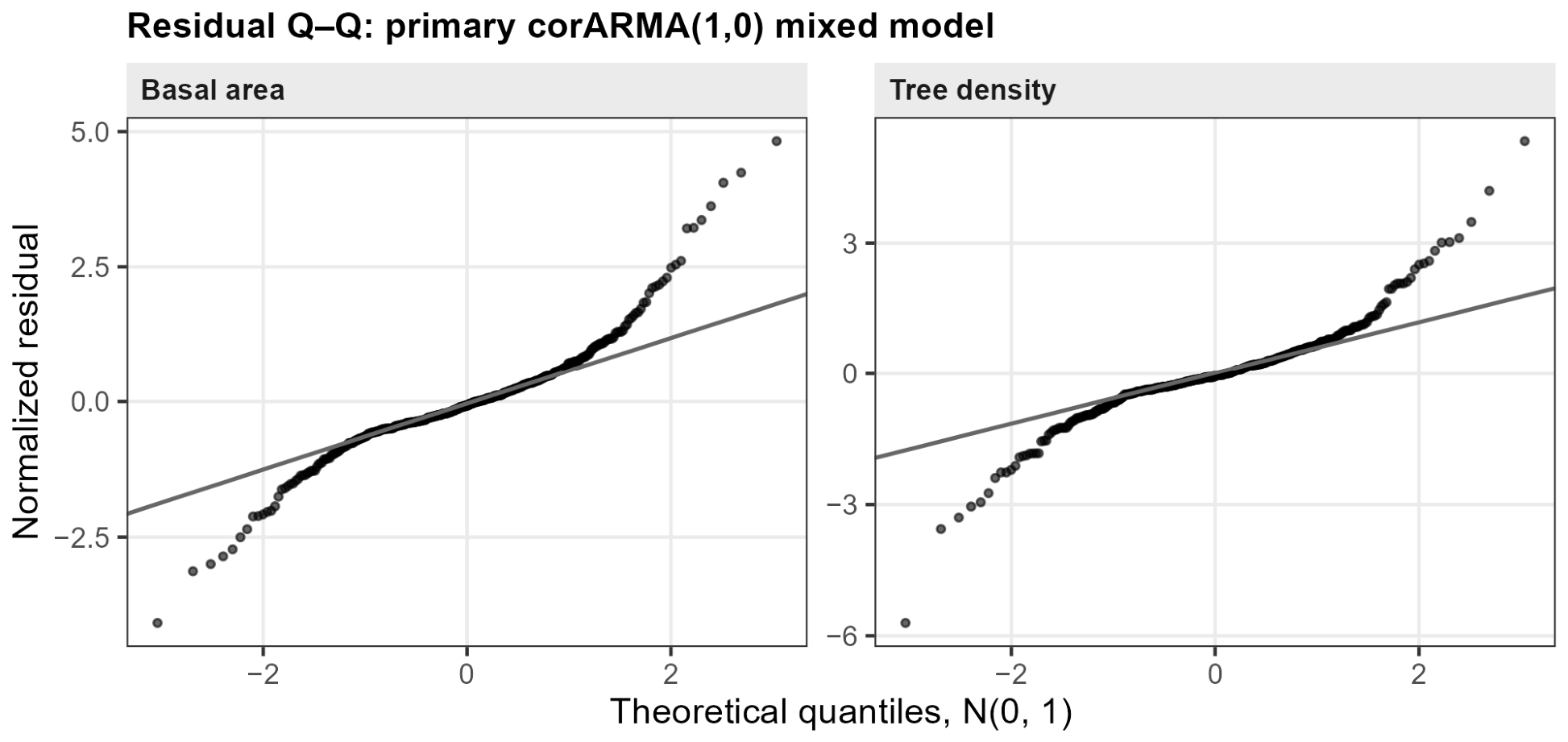
Figure A4.
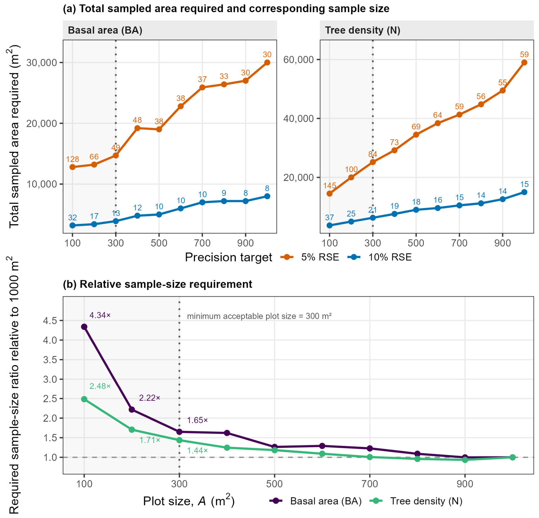
Projected sample size and total sampled area for 5% and 10% RSE scenarios across plot sizes. (a) Total sampled area required for the 5% and 10% RSE targets; numeric labels indicate the corresponding required number of plots. (b) Required sample-size ratio for basal area and tree density relative to the 1000 m2 design. In both panels, the vertical dotted line marks the 300 m2 minimum acceptable plot size. In panel (b), the horizontal dashed line at 1 indicates the same required sample size as the 1000 m2 design; values above 1 indicate a greater required number of plots. The figure complements the main-text Pareto presentation. Required sample sizes above 42 are projections that imply denser spatial sampling than was observed.
Appendix B. Supporting Diagnostic and Sensitivity Analyses
Appendix B.1. Mean-Effect and Agreement Diagnostics
The distribution-free Friedman test treated plot identity as the repeated-measures block and plot size as the within-plot factor. A complementary mixed-effects model was fitted by maximum likelihood with plot size as a categorical fixed effect, a random intercept for plot identity, and a first-order autoregressive [AR(1)] within-plot correlation structure over the ordered reconstructed plot sizes. The full model was compared with an intercept-only model by likelihood-ratio test. The analysis was repeated for all ten plot sizes and for the restricted range m2. Normal Q–Q plots of normalized residuals were used as the principal distributional diagnostic, with Shapiro–Wilk results reported only as a supporting check.
For formal equivalence, paired TOST used and a margin equal to ±10% of the 1000 m2 mean. A plot size was equivalent only when both one-sided tests rejected. The distribution-free equivalence companion resampled the 42 plot identities as paired units () and required the 90% percentile interval of the relative mean difference to lie entirely within ±10%. For the projected sample size needed by TOST, the observed paired mean difference and dispersion at were held fixed while was increased until the TOST half-width was small enough to satisfy the equivalence margin. This is a power/sensitivity calculation, not a prediction of the spatial variance under a denser future grid.
Multiplicity sensitivity for TOST used Bonferroni-adjusted one-sided significance levels. Family sizes of (the nine smaller plot sizes within an attribute) and (both attributes pooled) were examined in addition to the uncorrected tests.
Appendix B.2. Structural Diagnostics and the 200 m2 Radial Check
For the Donnelly edge-corrected Clark–Evans analysis, each 1000 m2 plot had radius . For a plot containing trees, the observed mean nearest-neighbor distance was . The expected distance under complete spatial randomness was
and the Clark–Evans index was . Values below 1 indicate clustering, 1 indicates complete spatial randomness, and values above 1 indicate regularity. Plots with at least five trees were used. The mean CE was compared with 1 using a one-sample test; Shapiro–Wilk and a Wilcoxon signed-rank test were reported as supporting distributional/robustness checks.
The local 200 m2 increase in the reconstructed means was examined with ten successive equal-area 100 m2 annuli. The principal paired test compared, within each of the 42 plots, the per-hectare value in the inner 200 m2 disc with that in the 200–1000 m2 outer annulus using a paired Wilcoxon signed-rank test. The annulus profile was also inspected to identify which 100 m2 band had the highest basal area and tree density. The calculation was repeated for fir stems only to assess whether non-fir species explained the local pattern.
At the 1000 m2 reference size, basal area and tree density were compared across the 42 plots using Pearson correlation with its 95% confidence interval; Spearman correlation was calculated as a rank-based companion.
Appendix B.3. Domain, Finite-Population, and Effort Sensitivity
The 90% fir-domain sensitivity was evaluated by excluding the retained borderline plot with 89.7% fir basal area and repeating the main plot-size calculations with . A separate domain-estimator check used all 48 selected plots. Let when plot satisfies the fir-domain criterion and 0 otherwise, and let . The domain mean was calculated as
with variance
where and . This was compared with the screened 42-plot estimate.
Finite-population sensitivity treated the estimated fir-domain area as a finite set of non-overlapping plots of size . For each plot size, was the corresponding number of possible plot-area units, where is in hectares, and the projected requirement was recalculated as
As an alternative measure of the variable field component, the expected number of trees measured under each design was calculated as , where is mean tree density at plot size . This comparison does not include travel, plot establishment, or other fixed per-plot costs.
Appendix B.4. Between-Plot Spatial Diagnostics
Between-plot spatial diagnostics used the 42 fir-domain plot centers. Moran’s was calculated for every attribute × plot-size combination using immediate grid neighbors within 350 m, which isolates the approximately 316 m first grid lag. Spatial weights were row-standardized, plots without a neighbor in a given distance band were retained with zero weight, and significance was assessed by 999 Monte Carlo permutations [32]. The 350 m cutoff lies between the largest observed immediate-neighbor separation and the smallest diagonal separation, so it isolates the intended first-lag neighbor set. A distance-band correlogram at the 1000 m2 reference used 0–350, 350–500, 500–700, and 700–1000 m bands.
A spatial block bootstrap was used as a consequence check rather than as a replacement variance estimator. Plot coordinates were partitioned by PAM into 14 spatially compact blocks (approximately three plots per block), and blocks were resampled as whole units for 2000 replicates. RSE interval widths were compared with those from an independent whole-plot bootstrap. Sensitivity to block definition was examined with 7, 10, 14, and 21 blocks. These diagnostics assess whether the SRS working approximation is visibly contradicted; they do not establish spatial independence. The corresponding interval-width results are reported in Section 3.6.
References
- Köhl, M.; Magnussen, S. Sampling in forest inventories. In Tropical Forestry Handbook; Pancel, L., Köhl, M., Eds.; Springer: Berlin/Heidelberg, Germany, 2016; pp. 777–837. [Google Scholar] [CrossRef] [Scilit]
- Cysneiros, V.C.; Vuolo, A.F.; Theodoroski, G.N.; Topanotti, L.R.; Pinho, L.C.; de Souza, E.L.; Pereira, I.R.S.; Proença, J.E.; Scipioni, M.C.; Bonazza, M.; et al. Assessing the influence of plot size and allometric model on carbon and tree diversity estimates in small Araucaria forest remnants. Environ. Monit. Assess. 2025, 197, 1025. [Google Scholar] [CrossRef] [Scilit] [PubMed]
- Pinto, L.O.R.; de Souza, C.R.; Terra, M.d.C.N.S.; de Mello, J.M.; Calegário, N.; Arcebi Júnior, F.W. Optimal plot size for carbon-diversity sampling in tropical vegetation. For. Ecol. Manag. 2021, 482, 118778. [Google Scholar] [CrossRef] [Scilit]
- Lombardi, F.; Marchetti, M.; Corona, P.; Merlini, P.; Chirici, G.; Tognetti, R.; Burrascano, S.; Alivernini, A.; Puletti, N. Quantifying the effect of sampling plot size on the estimation of structural indicators in old-growth forest stands. For. Ecol. Manag. 2015, 346, 89–97. [Google Scholar] [CrossRef] [Scilit]
- Fairfield Smith, H. An empirical law describing heterogeneity in the yields of agricultural crops. J. Agric. Sci. 1938, 28, 1–23. [Google Scholar] [CrossRef] [Scilit]
- Wagner, F.; Rutishauser, E.; Blanc, L.; Hérault, B. Effects of plot size and census interval on descriptors of forest structure and dynamics. Biotropica 2010, 42, 664–671. [Google Scholar] [CrossRef] [Scilit]
- Berrill, J.-P.; O’Hara, K.L. Influence of tree spatial pattern and sample plot type and size on inventory estimates for leaf area index, stocking, and tree size parameters. In Proceedings of the Coast Redwood Forests in a Changing California: A Symposium for Scientists and Managers (Gen. Tech. Rep. PSW-GTR-238, pp. 485–497); USDA Forest Service, Pacific Southwest Research Station: Albany, CA, USA, 2012. [Google Scholar]
- Gray, A. Monitoring stand structure in mature coastal Douglas-fir forests: Effect of plot size. For. Ecol. Manag. 2003, 175, 1–16. [Google Scholar] [CrossRef] [Scilit]
- Zeide, B. Plot size optimization. For. Sci. 1980, 26, 251–257. [Google Scholar] [CrossRef] [Scilit]
- Lynch, T.B. Optimal sample size and plot size or point sampling factor based on cost-plus-loss using the Fairfield Smith relationship for plot size. Forestry 2017, 90, 697–709. [Google Scholar] [CrossRef] [Scilit]
- Henttonen, H.M.; Kangas, A. Optimal plot design in a multipurpose forest inventory. For. Ecosyst. 2015, 2, 31. [Google Scholar] [CrossRef] [Scilit]
- Paul, T.S.H.; Kimberley, M.O.; Beets, P.N. Thinking outside the square: Evidence that plot shape and layout in forest inventories can bias estimates of stand metrics. Methods Ecol. Evol. 2019, 10, 381–388. [Google Scholar] [CrossRef] [Scilit]
- Kománek, M.; Knott, R.; Kadavý, J.; Kneifl, M. Is the concentric plot design reliable for estimating structural parameters of forest stands? Forests 2024, 15, 2246. [Google Scholar] [CrossRef] [Scilit]
- Musa, M.B.; Anik, C.S.; Emon, N.U.; Rahman, R.; Nila, T.M.; Datta, P.; Kilpeläinen, A.; Hassan, M.K.; Baul, T.K. Optimal plot size and shape for sampling growing stocks and tree species diversity in tropical forests: Results from a forest inventory in Hazarikhil Wildlife Sanctuary of Bangladesh. For. Ecol. Manag. 2025, 585, 122679. [Google Scholar] [CrossRef] [Scilit]
- Grussu, G.; Testolin, R.; Saulei, S.; Farcomeni, A.; Yosi, C.K.; De Sanctis, M.; Attorre, F. Optimum plot and sample sizes for carbon stock and biodiversity estimation in the lowland tropical forests of Papua New Guinea. Forestry 2016, 89, 150–158. [Google Scholar] [CrossRef] [Scilit]
- University Forest Administration and Management Fund (UFAMF). Pertouli University Forest Management Plan 2019–2028; Aristotle University of Thessaloniki: Thessaloniki, Greece, 2018. [Google Scholar]
- Matis, K. Forest Biometrics: II. Dendrometry; Pegasus: Thessaloniki, Greece, 2004; Volume 2, 674p. (In Greek) [Google Scholar]
- Matis, K. Sampling of Natural Resources; Pegasus: Thessaloniki, Greece, 2004; 525p. (In Greek) [Google Scholar]
- Ministry of Environment and Energy; General Secretariat for Forests. Υ.A. ΥΠΕΝ/ΔΠΔΠ/129246/6285/25-11-2024: Επικαιροποίηση τεχνικών προδιαγραφών εκπόνησης δασοπονικών μελετών διαχείρισης δασών και δασικών οικοσυστημάτων (ΦΕΚ 6930/Β/2024) [Ministerial Decision ΥΠΕΝ/ΔΠΔΠ/129246/6285/25-11-2024: Update of the technical specifications for the preparation of forest management studies for forests and forest ecosystems]. Government Gazette of the Hellenic Republic, Issue B 6930, 18 December 2024. 2024. Available online: https://geotee.gr/2024/12/19/y-a-ypen-dpdp-129246-6285-25-11-2024-epikairopoiisi-technikon-prodiagrafon-ekponisis-dasoponikon-meleton-diacheirisis-dason-kai-dasikon-oikosystimaton-fek-6930-v-2024/ (accessed on 18 August 2026).
- Adolt, R.; Maděra, P.; Abraham, J.; Čupa, P.; Svátek, M.; Matula, R.; Šebesta, J.; Čermák, M.; Volařík, D.; Koutecký, T.; et al. Field survey of Dracaena cinnabari populations in Firmihin, Socotra Island: Methodology and preliminary results. J. Landsc. Ecol. 2013, 6, 7–34. [Google Scholar] [CrossRef] [Scilit]
- Field-Map; Hardware and Software Technology for Spatial Forest Data Collection [Computer Software]; IFER—Monitoring and Mapping Solutions Ltd.: Jílové u Prahy, Czech Republic, 2026. Available online: https://www.field-map.com (accessed on 5 July 2026).
- Kershaw, J.A.; Ducey, M.J.; Beers, T.W.; Husch, B. Forest Mensuration, 5th ed.; John Wiley & Sons: Hoboken, NJ, USA, 2016. [Google Scholar] [CrossRef] [Scilit]
- Magnussen, S.; McRoberts, R.E.; Breidenbach, J.; Nord-Larsen, T.; Ståhl, G.; Fehrmann, L.; Schnell, S. Comparison of estimators of variance for forest inventories with systematic sampling—Results from artificial populations. For. Ecosyst. 2020, 7, 17. [Google Scholar] [CrossRef] [Scilit]
- Lin, L.I.-K. A concordance correlation coefficient to evaluate reproducibility. Biometrics 1989, 45, 255–268. [Google Scholar] [CrossRef] [Scilit]
- Schuirmann, D.J. A comparison of the two one-sided tests procedure and the power approach for assessing the equivalence of average bioavailability. J. Pharmacokinet. Biopharm. 1987, 15, 657–680. [Google Scholar] [CrossRef] [Scilit] [PubMed]
- Angelis, L.; Stamatellos, G. Multiple objective optimization of sampling designs for forest inventories using random search algorithms. Comput. Electron. Agric. 2004, 42, 129–148. [Google Scholar] [CrossRef] [Scilit]
- Kaufman, L.; Rousseeuw, P.J. Finding Groups in Data: An Introduction to Cluster Analysis; John Wiley & Sons: Hoboken, NJ, USA, 1990. [Google Scholar] [CrossRef] [Scilit]
- Georgakis, A.; Gatziolis, D.; Stamatellos, G. A primer on clustering of forest management units for reliable design-based direct estimates and model-based small area estimation. Forests 2023, 14, 1994. [Google Scholar] [CrossRef] [Scilit]
- Clark, P.J.; Evans, F.C. Distance to nearest neighbor as a measure of spatial relationships in populations. Ecology 1954, 35, 445–453. [Google Scholar] [CrossRef] [Scilit]
- Donnelly, K. Simulations to determine the variance and edge-effect of total nearest neighbour distance. In Simulation Studies in Archaeology; Hodder, I., Ed.; Cambridge University Press: Cambridge, UK, 1978; pp. 91–95. [Google Scholar]
- Pinheiro, J.C.; Bates, D.M. Mixed-Effects Models in S and S-PLUS; Springer: Berlin/Heidelberg, Germany, 2000. [Google Scholar] [CrossRef] [Scilit]
- Bivand, R.S.; Wong, D.W.S. Comparing implementations of global and local indicators of spatial association. Test 2018, 27, 716–748. [Google Scholar] [CrossRef] [Scilit]
- Stamatellos, G.S. Comparison of Point and Point-3P sampling for forest volume estimation with cost analysis. For. Ecol. Manag. 1995, 74, 75–79. [Google Scholar] [CrossRef] [Scilit]
- Stamatellos, G.; Blioumis, V. Optimization of the forest volume estimation with plot-double sampling when there is a walking cost of the second-phase sample. MEDIT 1997, 8, 23–26. [Google Scholar]
- Hynynen, J.; Ojansuu, R. Impact of plot size on individual-tree competition measures for growth and yield simulators. Can. J. For. Res. 2003, 33, 455–465. [Google Scholar] [CrossRef] [Scilit]
- Rodríguez-Ruiz, J.; Martínez-Calvo, A.; Pérez-Cruzado, C. Designing circular fixed-area plots in large-scale forest inventories: Effect of horizontal distance measurement uncertainty and tree position pattern. Can. J. For. Res. 2025, 55, 1–14. [Google Scholar] [CrossRef] [Scilit]
- Mandallaz, D. Sampling Techniques for Forest Inventories; Chapman & Hall/CRC: Boca Raton, FL, USA, 2008. [Google Scholar] [CrossRef] [Scilit]
- Georgakis, A.; Diamantopoulou, M.J. Diagnosing inconsistency in compartment-level growing stock volume estimates across inventory methodological transitions: Evidence from a Greek uneven-aged forest. Forests 2026, 17, 755. [Google Scholar] [CrossRef] [Scilit]

Disclaimer/Publisher’s Note: The statements, opinions and data contained in all publications are solely those of the individual author(s) and contributor(s) and not of MDPI and/or the editor(s). MDPI and/or the editor(s) disclaim responsibility for any injury to people or property resulting from any ideas, methods, instructions or products referred to in the content. |
© 2026 by the authors. Licensee MDPI, Basel, Switzerland. This article is an open access article distributed under the terms and conditions of the Creative Commons Attribution (CC BY) license.