Spatial Equity of Green-Space Provision in Chinese Megacities: Nonlinear Associations with Urban Morphology Across Three Temporal Snapshots (2015–2025)

Abstract

Against the backdrop of stock-space urban renewal, green-space governance in megacity cores increasingly requires a shift from expansion-oriented supply to the optimisation of existing spatial resources. This study examines the spatial equity of green-space provision in the central districts of seven Chinese megacities using high-resolution remote-sensing data from 2015, 2020, and 2025. We combined semantic segmentation, nested-buffer measurement, the Gini coefficient, Extreme Gradient Boosting (XGBoost), and Shapley Additive Explanations (SHAP) to evaluate the relationships between urban morphology and green-space provision. We first derived a pixel-level cumulative green-space provision index from nested-buffer measurements and calculated city-year Gini coefficients to quantify distributional inequality. XGBoost models were then used to predict the cumulative green-space provision index from urban morphology, and SHAP was applied to interpret the resulting nonlinear, model-derived associations. The results show that changes in the green-space provision index and its distributional inequality were not synchronous across cities. Beijing showed the largest increase in inequality, whereas Chengdu showed the strongest improvement; Tianjin recorded the fastest increase in the green-space provision index, while Beijing experienced a marked decline. Urban form showed nonlinear associations with the unit-level green-space provision index, helping to explain the spatial differentiation underlying the city-year Gini coefficients. Building density was the primary contributor in most city-year models, whereas compactness showed threshold-like associations, with positive effects at lower levels and inhibitory effects at higher levels. Statistical testing and clustering further indicated substantial heterogeneity among cities, which were categorised into three spatial patterns: centripetal agglomeration, peripheral expansion, and clustering/ring-shaped fluctuation. These findings provide morphology-based evidence for differentiated green-space governance in high-density megacity cores, though they should not be interpreted as a complete socioeconomic assessment of green-space equity.

1. Introduction

The central areas of China’s megacities are undergoing a transition from a phase of incremental expansion towards one of stock-oriented urban renewal. Over an extended period, spatial expansion driven by construction efficiency has, to varying degrees, encroached upon ecological space. The continued conversion of ecological land into construction land has contributed to the fragmentation of green spaces, reduced spatial connectivity, and declining ecosystem service capacity [1,2,3]. As a result, the tension between high-density built environments and limited ecological resources has become increasingly pronounced, further intensifying inequalities in access to ecological resources [4,5,6]. Within the context of stock-oriented renewal, the challenge of achieving equitable green-space governance therefore extends beyond simply increasing green-space quantity and increasingly involves improving the spatial-allocation efficiency of limited ecological resources through optimisation of the existing built environment [7,8].

As a key spatial manifestation of the built environment, urban form has been widely recognised as an important factor influencing the distribution pattern and equity of green-space provision [9,10]. Existing studies have primarily examined the relationship between the built environment and green-space distribution using two-dimensional indicators, such as building density, floor-area ratio, and land development intensity [11,12]. With advances in remote sensing and spatial analysis technologies, increasing attention has been directed towards more complex morphological characteristics, including three-dimensional structural configurations, street canyon morphology, and spatial compactness [13,14]. Previous studies have suggested that urban form may influence green-space provision not only through geometric constraints on spatial layout but also through spatial connectivity, surface roughness, and the degree of functional mixing, all of which are associated with the efficiency of ecological resource allocation [15,16,17]. This indicates that the spatial equity of green-space provision in high-density cities is not solely associated with the total amount of green space. It is also related to the way limited green-space resources are distributed relative to spatial structure, development intensity, and functional organisation during urban morphological evolution [18]. Therefore, in this study, equity refers to the spatial distribution of green-space provision rather than to the full socioeconomic dimensions of green-space justice.

Although previous research has explored the relationship between urban form and green-space provision, most studies remain grounded in linear analytical assumptions, whereby the effects of morphological variables on green-space equity are considered stable and uniform [19]. In recent years, however, the increasing application of machine learning and interpretable modelling approaches has revealed that the ecological effects of morphological indicators often exhibit substantial non-linear characteristics as development intensity increases [20,21,22]. For example, building density may contribute to spatial agglomeration and resource-sharing efficiency at relatively low levels, whereas beyond certain thresholds, it may correspond to ecological space compression and greater unevenness in green-space distribution [23]. Nevertheless, much of the existing research remains limited to static analyses based on single time points, with comparatively limited attention paid to how model-based associations between urban form and green-space provision vary across comparable time snapshots [24].

In practice, urban form is inherently dynamic and continuously evolves through processes such as urban renewal, population mobility, and functional reorganisation [13,25]. Accordingly, associations between urban form and green-space provision may differ across urban-development contexts and observation years [24]. Changes in urban spatial structure are often accompanied by ongoing reconfigurations of population activities, land use patterns, and functional organisation, which may, in turn, reshape the allocation logic of ecological resources [2,26]. However, few studies have systematically compared model-derived associations across multiple consistently defined observation years. Most existing analyses assess morphology–environment relationships at a single time point, whereas comparatively few studies have examined how morphology-related response patterns differ across comparable temporal snapshots and urban-development contexts [21,24]. In addition, existing research has predominantly concentrated on individual cities or localised regions, with relatively limited cross-city comparative analysis. As a result, many findings remain insufficient in terms of explaining broader patterns under varying development stages and spatial structures. This issue is particularly relevant in the context of China’s megacities, where substantial differences exist in development stage, central area density, and functional organisation, potentially resulting in considerable heterogeneity in the mechanisms shaping the spatial equity of green-space provision [8,27]. Consequently, an analytical framework is needed that integrates multidimensional morphological indicators, multi-temporal observations, and cross-city comparisons to examine the nonlinear associations between urban morphology and the spatial equity of green-space provision.

To address these gaps, this study focuses on the central districts of seven megacities: Beijing, Shanghai, Guangzhou, Shenzhen, Tianjin, Chongqing, and Chengdu. Using remote-sensing data from 2015, 2020, and 2025, we employ the Gini coefficient to characterise the spatial equity of green-space provision. A multidimensional urban-form indicator system incorporating building geometry, spatial compactness, and functional activity is constructed, and XGBoost is applied in combination with SHAP to examine nonlinear, model-based associations between urban morphology and green-space provision [20,28]. The contributions of this study are threefold. First, it develops a morphology-oriented analytical framework for assessing spatial inequalities in green-space provision within high-density urban cores. Second, by comparing three observation years, it illustrates how the relationships between urban form and green-space provision vary across different time points. Third, through cross-city comparison, it identifies differentiated spatial characteristics that can support context-specific strategies for equitable green-space planning and governance.

2. Study Area and Data

2.1. Study Area

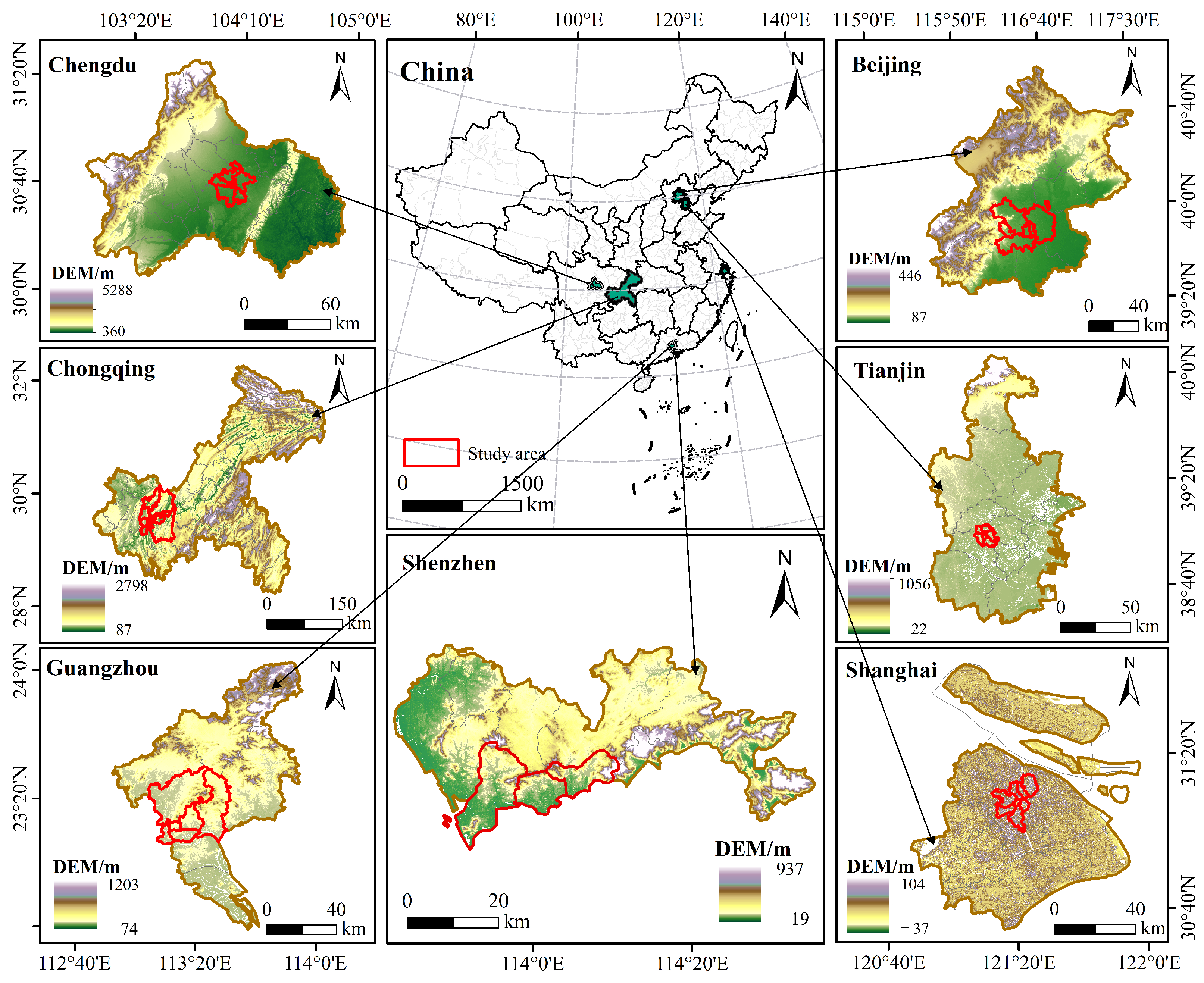
This study selected Beijing, Shanghai, Guangzhou, Shenzhen, Tianjin, Chongqing, and Chengdu as the sample cities (Figure 1). These seven cities represent not only the major growth poles of China’s socio-economic development but also some of the most highly urbanised and spatially complex metropolitan areas in contemporary China [26]. From a national strategic perspective, they encompass the core engines of the Beijing–Tianjin–Hebei region, the Yangtze River Delta, the Pearl River Delta, and the Chengdu–Chongqing Dual-City Economic Circle and occupy important positions within China’s political, economic, and cultural systems. The selection of these cities was primarily motivated by their strong socio-economic representativeness. Characterised by exceptionally high concentrations of population and capital, these megacities have experienced substantial benefits associated with rapid urban growth while also facing increasing pressures related to land scarcity and population agglomeration [29]. Owing to differences in development trajectories and industrial structures, the selected cities exhibit diverse socio-spatial configurations, including historically developed global urban centres, rapidly expanding compact urban districts, and clustered urban spaces shaped by topographic conditions. This diversity provides a useful comparative basis for examining spatial differences in green-space provision [30,31]. For each megacity, the study area was defined as a rectangular analytical extent covering the officially designated administrative central districts identified from municipal master plans or territorial spatial master plans. The same boundaries were used for 2015, 2020, and 2025 to ensure temporal comparability.

2.2. Data Extraction

This study selected historical Google Earth imagery as the primary remote-sensing data source to balance spatial resolution, temporal consistency, and regional coverage. To minimise the influence of seasonal vegetation phenology on green-space identification, imagery was consistently selected during the stable growing season (May–October) for each study year. Image acquisition dates and study-area information for all cities are summarised in Appendix A. Historical Google Earth imagery is composed of mosaics compiled from multiple commercial satellite providers; therefore, the Google Earth Historical Imagery platform is uniformly reported as the imagery source throughout this study. After quality screening, high-resolution RGB imagery (0.6 m spatial resolution, 24-bit depth, and three spectral bands) was obtained for the three study years (2015, 2020, and 2025). Because the imagery was acquired under different sensors and acquisition conditions, cloud-free scenes with minimal seasonal differences were preferentially selected, and stable urban features (e.g., major road intersections and landmark buildings) were used for visual co-registration to improve spatial consistency among observation years [32]. Since Google Earth imagery does not provide radiometrically calibrated surface reflectance, radiometric correction was not performed, and all images were processed using a consistent visual interpretation protocol throughout the study.

Night-time light intensity (NTL) was derived from the NOAA/VIIRS/DNB/MONTHLYV1/VCMCFG monthly cloud-free composite product available on the Google Earth Engine platform. Annual composites were generated by averaging monthly observations for 2015, 2020, and 2025 using the avg_rad band. The annual composites were directly aligned with the analytical grid at the nominal spatial resolution (approximately 500 m), and the mean NTL value for each analytical unit was calculated using the reduceRegions function with a mean reducer. The extracted imagery was subsequently used for semantic segmentation to identify buildings and green spaces, and the resulting building layer served as the basis for calculating urban morphological indicators.

3. Methodology

3.1. Methodological Workflow

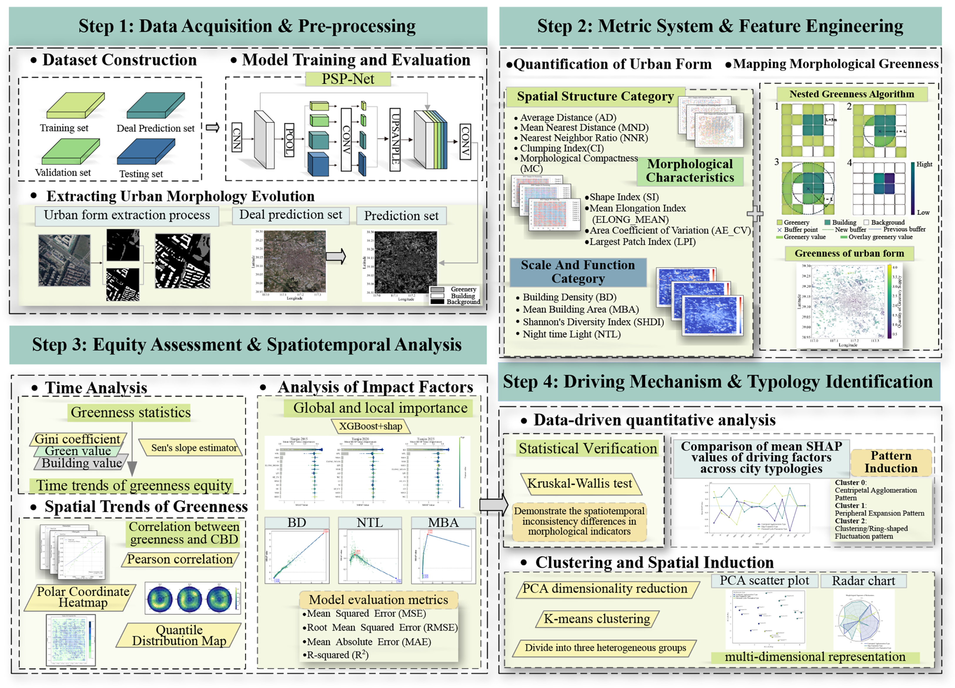
This study established a progressive framework encompassing feature extraction, association analysis, and spatial typology classification (Figure 2). First, building and green-space features for 2015, 2020, and 2025 were extracted using PSPNet, and multi-scale green-space provision was characterised through nested-buffer analysis. Second, an urban-form indicator system was constructed to capture spatial structure, morphological characteristics, and functional scale. Third, the Gini coefficient was used to characterise the spatial equity of green-space provision, while Pearson correlation analysis and the XGBoost–SHAP framework were used to explore nonlinear, model-based associations between morphological factors and the provision index. Finally, significance testing and PCA–K-means clustering were used to classify differentiated spatial patterns across cities. Overall, this framework supported a systematic multi-source analysis and an association-based interpretation rather than causal identification.

3.2. Semantic Segmentation and Urban Morphological Indicator Framework

In terms of urban pattern recognition, this study employed the Pyramid Scene Parsing Network (PSPNet) as the semantic segmentation model for extracting buildings and green spaces from high-resolution remote-sensing imagery [33,34]. The model was implemented using Python 3.10 and the PyTorch v2.12.1 deep-learning framework and trained on a workstation equipped with an Intel Core Ultra 7 265K CPU and an NVIDIA GeForce RTX 5060 Ti (16 GB) GPU. A ResNet-101 backbone was adopted as the feature extractor, and a Pyramid Pooling Module (PPM) was incorporated to aggregate contextual information at multiple spatial scales, thereby improving the representation of complex urban structures. Multi-scale pooled features were compressed using convolution, upsampled, and fused with high-resolution feature maps to generate the final semantic segmentation results [35]. The network received RGB image tiles ($1024\times 1024$ pixels) as input, and two semantic classes—namely, Buildings and Green Spaces—were consistently defined throughout the study.

To improve model generalisation across multi-temporal imagery, a two-stage transfer-learning strategy was adopted. The model was first pre-trained on the publicly available INRIA and UGS-1M datasets and subsequently fine-tuned using a locally annotated dataset [36,37,38,39]. The multi-temporal dataset contained 52,800 image patches, of which 1056 patches were manually annotated in LabelMe by five trained annotators following a standard two-class interpretation protocol for model fine-tuning and validation. Buildings were defined as permanent building footprints, whereas green spaces included trees, shrubs, grasslands, parks, and other continuous vegetated surfaces. Bare soil, agricultural land, water bodies, transportation infrastructure, and shadow areas were treated as background. Green roofs were excluded because they could not be consistently identified from historical Google Earth imagery, and mixed pixels were assigned to the dominant visual class. All annotations were independently reviewed by the corresponding author, and disagreements were resolved through consensus-based visual interpretation. The manually annotated dataset was partitioned into a training set (70%, $n=739$) and a validation set (30%, $n=317$) using spatial cross-validation, in which mutually non-overlapping spatial blocks were assigned to the two subsets to prevent spatial data leakage caused by adjacent samples appearing in both the training and validation sets. This partitioning strategy balanced the sample diversity required for model training with the stability of validation results while ensuring that all seven cities and three observation years were represented in both subsets. The validation set was used exclusively for model evaluation and was not involved in parameter optimisation or model updating. Model performance was evaluated using accuracy, F1 score, the Kappa coefficient, and mean Intersection-over-Union (mIoU).

Table 1. Performance comparison before and after model fine-tuning. The last row reports the performance improvement ($\mathsf{\Delta }=\mathrm{Fine}\text{-}\mathrm{tuning}-\mathrm{Pre}\text{-}\mathrm{training}$).

Training Stage	Accuracy	F1 Score	Kappa	mIoU
Pre-training	0.901235	0.731405	0.462883	0.622537
Fine-tuning	0.967438	0.908263	0.816527	0.840325
Improvement ($\mathsf{\Delta }$)	0.066203	0.176858	0.353644	0.217788

presents the results before and after fine-tuning, together with the corresponding absolute improvement ($\mathsf{\Delta }=\mathrm{Fine}\text{-}\mathrm{tuning}-\mathrm{Pre}\text{-}\mathrm{training}$), and the definitions of all evaluation metrics are provided in Appendix B.

Having obtained the spatial distributions of buildings and green spaces, we transformed the semantic-segmentation outputs into quantitative descriptors of the built environment for subsequent association analysis. Specifically, a multidimensional urban morphological indicator framework was established across three complementary dimensions—namely, spatial structure, morphological characteristics, and functional scale (

Table 2. Description of urban morphology indicators.

Dimension	Indicator	Calculation Formula	Indicator Significance
Spatial Structure	Average Distance (AD)	$AD={\displaystyle \frac{1}{N(N-1)}}{\sum }_{i=1}^N{\sum }_{j\ne i}^N{d}_{ij}$	This measures the overall concentration of buildings; a lower value indicates greater concentration.
	Mean Nearest Distance (MND)	$MND={\displaystyle \frac{1}{N}}{\sum }_{i=1}^N{d}_i$	A measure of the distance between the nearest neighbours in a building; a smaller value indicates a more compact distribution.
	Nearest-Neighbour Ratio (NNR)	$NNR={\displaystyle \frac{{\overline{d}}_{obs}}{{\overline{d}}_{rand}}}$ $d_{rand}={\displaystyle \frac{1}{2\sqrt{\frac{N}{A_{total}}}}}$	Determines building distribution patterns: <1 indicates clustering, =1 indicates random distribution, >1 indicates uniform distribution.
	Clumping Index (CI)	$CI={\displaystyle \frac{{\sum }_{i=1}^N{A}_i}{A_{convex}}}$	A measure of the degree to which a group of buildings fills the space; the higher the value, the more compact the group.
	Morphological Compactness (MC)	$MC={\displaystyle \frac{2\sqrt{\pi A_i}}{P_i}}$	A measure of a building’s compactness; the closer the value is to 1, the more regular the shape.
Morphological Characteristics	Shape Index (SI)	$S{I}_i={\displaystyle \frac{P_i}{2\sqrt{\pi A_i}}}$ $SI={\displaystyle \frac{1}{N}}{\sum }_{i=1}^{N}S{I}_i$	This reflects the complexity of a building’s shape; the higher the value, the more irregular the shape.
	Mean Elongation Index (ELONG_MEAN)	$ELON{G}_{MEAN}={\displaystyle \frac{1}{N}}{\sum }_{i=1}^N{\displaystyle \frac{L_i}{W_i}}$	A measure of the building’s overall extent; the higher the value, the more elongated the building.
	Area Coefficient of Variation (AE_CV)	$AE\_CV={\displaystyle \frac{{\sigma }_A}{\overline{A}}}$ ${\sigma }_A=\sqrt{{\displaystyle \frac{1}{N}}{\sum }_{i=1}^N{(A_i-\overline{A})}^2}$	This measures the heterogeneity of floor area; the higher the value, the more pronounced the variation.
	Largest Patch Index (LPI)	$LPI={\displaystyle \frac{A_{max}}{A_{total}}}\times 100$	Reflects the extent to which the largest building dominates the space.
Functional Scale	Building Density (BD)	$BD={\displaystyle \frac{{\sum }_{i=1}^N{A}_i}{A_{total}}}$	A measure of building coverage and development density; the higher the value, the more compact the development.
	Mean Building Area (MBA)	$MBA={\displaystyle \frac{1}{N}}{\sum }_{i=1}^N{A}_i$	Reflects the average size of buildings.
	Shannon’s Diversity Index (SHDI)	$SHDI=-{\sum }_{j=1}^m{p}_{j}ln{p}_j$	Measures the diversity and uniformity of building types.
	Night-time Light (NTL)	$NTL={\displaystyle \frac{1}{n}}{\sum }_{i=1}^n{L}_i$	Reflects the intensity of human activity and the level of urbanisation.

Notes: N: number of buildings; $d_{ij}$: the distance between building i and building j; $d_i$: the distance from building i to its nearest neighbour; ${\overline{d}}_{obs}$: observed average nearest-neighbour distance; $d_{rand}$: average distance in a random distribution; $A_{total}$: area of the study region; $A_i$: the floor area of the i-th building; $A_{convex}$: convex hull area of a set of buildings; $P_i$: the perimeter of the i-th building; $L_i$: the brightness value of the i-th pixel; $W_i$: the length of the short axis of the i-th building; $\overline{A}$: average floor area; ${\sigma }_A$: standard deviation of floor area; $A_{max}$: maximum building-plot area; $p_j$: proportion of buildings in category j; m: number of types; n: number of pixels.

) [40,41]. Spatial-structure indicators describe the organisation and aggregation patterns of building units, reflecting their potential influence on green-space distribution and accessibility. Morphological-characteristic indicators quantify geometric complexity and spatial configuration, thereby characterising the embedding patterns of green spaces within high-density urban environments. Functional-scale indicators represent urban development intensity and spatial carrying capacity, providing quantitative support for analysis of the interactions among building development, green-space provision, and spatial competition [42,43]. Together with the night-time light (NTL) variable, these indicators served as explanatory variables in the subsequent XGBoost-SHAP analysis to predict the cumulative green-space provision index and interpret nonlinear model-derived associations.

3.3. Assessment Methods for Green-Space Equity and Spatio-Temporal Dynamics

To characterise the spatial-provision dimension of green-space equity, this study introduced a nested-buffer approach that measures how green spaces are distributed around built-up activity units [44,45]. Unlike fixed-distance buffers (e.g., 500 m or 1000 m), this approach incorporates multiple nested Euclidean distance bands; while closer green-space patches are inherently counted across multiple overlapping bands, this cumulative summation intentionally reflects multi-scale availability and assigns greater representation to nearby green spaces, which are generally associated with higher potential environmental and social benefits [46]. Consequently, the resulting metric is interpreted as a relative, cumulative spatial provision index rather than a physical, non-overlapping measurement of green-space area, representing spatial proximity and potential supply rather than realised pedestrian accessibility through the actual street network.

In this study, building footprints were defined as human activity zones, while vegetated areas within the city were identified as green spaces. The analytical procedure consisted of three main steps. First, to improve computational efficiency, pixels with a spatial resolution of $L=5$ m were adopted as the basic analytical units, and building data at time point $S_t$ were converted into spatial variables ($Z_{i,t}$) through grid segmentation. Second, both the initial buffer radius (r) and the step size (l) were set to 5 m, and 400 iterative calculations ($k=0,\dots ,399$) were performed under the constraint of a maximum radius of $R=2000$ m. Finally, by progressively accumulating the intersection area between buffer zones and green spaces for each analytical unit during each iteration cycle, the utility of green-space provision was quantitatively characterised [47,48]. The calculation formula is expressed as follows:

$$A_{i,t}={\displaystyle \sum _{k=0}^{399}}\mathrm{Area}\left(\mathrm{Buffer}\left(Z_{i,t},r+k·l\right)\cap G_t\right),k=0,1,2,\dots ,399$$

(1)

Here, $A_{i,t}$ denotes the cumulative green-space provision index for the i-th impervious artificial-surface pixel ($Z_{i,t}$) at time step t. It is calculated by progressively intersecting green spaces ($G_t$) with concentric buffer zones ($\mathrm{Buffer}(Z_{i,t},r+k·l)$) centred on the pixel. Because these buffers are nested, a single green-space patch can contribute to multiple distance bands; thus, $A_{i,t}$ functions as a cumulative provision metric rather than a direct measure of physical area.

The formula to calculate the state of green-space equity in a city at a given point in time is expressed as follows:

$$\overline{A_t}={\displaystyle \frac{1}{n}}{\displaystyle \sum _{i=1}^n}{A}_{i,t}$$

(2)

$$Gin{i}_t=1+{\displaystyle \frac{1}{n}}-{\displaystyle \frac{2}{\overline{A_t}·n^2}}{\displaystyle \sum _{i=1}^n}\left[(n-i+1)·A_{i,t}\right]$$

(3)

${\mathrm{Gini}}_t$ represents the degree of inequality in the distribution of the pixel-level cumulative green-space provision index within the study area at time t, ${\overline{A}}_t$ denotes the mean pixel-level cumulative green-space provision index calculated from all building pixels at time t, and n represents the total number of building pixels within the city boundary at time t.

Temporal changes in the city-level cumulative green-space provision index, the Gini coefficient, and the total number of building pixels across the three observation years (2015, 2020, and 2025) were characterised using Sen’s slope estimator. The city-level cumulative green-space provision index was obtained by summing the pixel-level cumulative green-space provision index across all building pixels within each city, whereas the Gini coefficient was calculated from the distribution of the pixel-level $A_{i,t}$ values. Sen’s slope estimator is a widely used non-parametric method for describing the direction and magnitude of temporal change [49,50]. Because this study is based on three discrete observation years rather than a continuous annual time series, the estimator was used to characterise the directional changes between observation years rather than to infer long-term temporal trends. The calculation formula is expressed as follows:

$$\left\{\begin{array}{c}{S}_{uj}={\displaystyle \frac{W_{t_j}-W_{t_u}}{t_j-t_u}}\hfill \\ Sen=\mathrm{median}(S_1,S_2,\dots ,S_m)\hfill \\ m={\displaystyle \frac{n(n-1)}{2}}\hfill \end{array}\right.$$

(4)

Here, $S_{uj}$ denotes the slope calculated between two observation years $(t_u,t_j)$, $Sen$ is the median of all pairwise slopes, m is the total number of pairwise slope estimates, and $W_t$ represents the value of the indicator at observation year t. Depending on the analysis, $W_t$ refers to the city-level cumulative green-space provision index, the city-year Gini coefficient, or the total number of building pixels. In the present three-snapshot design, a positive Sen slope indicates an increasing trend between observation years, whereas a negative value indicates a decreasing trend. Values close to zero indicate relatively small directional changes. Owing to the limited number of observation years, the estimated slope should be interpreted as a descriptive measure of change rather than a statistically robust long-term trend.

3.4. Explainable Machine Learning: XGBoost-SHAP

XGBoost (Extreme Gradient Boosting) is a gradient-boosting framework widely applied in machine-learning tasks [51]. One of its major advantages lies in its capacity to capture complex non-linear relationships while maintaining a certain degree of model interpretability [52]. In the analysis of multiple factors influencing urban green-space equity, XGBoost demonstrates strong non-linear fitting capability, allowing the interactions among variables to be examined more effectively [51]. The loss function of XGBoost consists of an empirical loss term and a regularisation term, which are used to measure the discrepancy between predicted and observed values, as well as the complexity of the model:

$$obj\left(\theta \right)={\displaystyle \sum _{i=1}^n}L(y_i,{\widehat{y}}_i)+{\displaystyle \sum _{k=1}^K}\mathsf{\Omega }\left(f_k\right)$$

(5)

In this context, ${\sum }_{i=1}^{n}L(y_i,{\widehat{y}}_i)$ represents the empirical loss term, which quantifies the loss between the predicted and true values in the training data; ${\sum }_{k=1}^K\mathsf{\Omega }\left(f_k\right)$ represents the regularisation term, which denotes the sum of the complexities of all K trees and is used to control model overfitting; $L(y_i,{\widehat{y}}_i)$ denotes the loss value for the i-th sample; $\mathsf{\Omega }\left(f_k\right)$ denotes the complexity of the k-th base model; and $\theta$ denotes the model parameters.

SHAP (Shapley Additive Explanations) is an interpretable machine-learning method used to explain model predictions [53]. Based on the Shapley value derived from cooperative game theory, SHAP quantifies the contribution of each feature to the model output by calculating its marginal effect across different combinations of feature subsets. By considering all possible feature combinations, the method provides a relatively consistent and balanced allocation of feature contributions. In this framework, an increase in the marginal influence of a feature on model output corresponds to a non-decreasing contribution value, thereby improving the stability and reliability of the results of model interpretation [54,55].

Let N denote the set of all attributes, and let $n=\left|N\right|$ denote the total number of attributes. The Shapley value (${\varphi }_i$) for any attribute i is defined as the weighted average of its marginal contributions across all subsets ($S\subseteq N$) that do not contain that attribute, i.e.,

$$\left\{\begin{array}{c}{\displaystyle {\varphi }_i=\sum _{S\subseteq N\setminus \left\{i\right\}}\frac{\left|S\right|!(n-|S|-1)!}{n!}[f(S\cup \left\{i\right\})-f\left(S\right)]}\hfill \\ {\displaystyle g\left(z^{\prime }\right)={\varphi }_0+{\displaystyle \sum _{i=1}^M}{\varphi }_i{z}_i^{\prime }}\hfill \end{array}\right.$$

(6)

Here, ${\varphi }_i$ is the Shapley value of explanatory variable i, representing the contribution of explanatory variable i. n denotes the total number of morphological indicators in the input model. $f(S\cup \{i\left\}\right)$ denotes the model result when explanatory variable i is included. $f\left(S\right)$ denotes the model result when explanatory variable i is excluded. $g\left(z^{\prime }\right)$ is the model output, i.e., the predicted value. $z^{\prime }$ is used to indicate whether the explanatory variable is observed, M is the number of input features, and ${\varphi }_0$ is the baseline value.

For each city-year, an XGBoost regression model was fitted with analytical units as samples, urban-form indicators as predictors, and the cumulative green-space provision index ($A_{i,t}$) as the response variable. The city-year Gini coefficient was not used as the model response; it was calculated separately to summarise the inequality of $A_{i,t}$ across analytical units. The dataset was randomly partitioned into training and test sets at an 8:2 ratio. Grid-search cross-validation was subsequently applied to optimise model hyperparameters, thereby enhancing model stability and generalisation performance [56]. Upon determination of the optimal parameter combination, the model was executed to generate predictions for the test set, with its performance rigorously evaluated using $R^2$ and RMSE (see Appendix B). Furthermore, the SHAP method was introduced to interpret the model outputs and rank feature contributions. In this framework, the sign of a SHAP value indicates whether a variable is positively or negatively associated with the prediction, while its absolute value reflects the relative magnitude of that model-based contribution. Crucially, these SHAP values are interpreted strictly as predictive associations within the fitted model rather than causal effects; in instances where model performance was relatively low, the corresponding SHAP results were treated as purely exploratory.

To identify the integrated characteristics of multi-dimensional urban morphology and classify spatial patterns, this study adopted a combined PCA–K-mean analytical framework. First, Principal Component Analysis (PCA) was used to reduce the dimensionality of the 13 morphological indicators, transforming redundant information into mutually independent composite variables [57]. Subsequently, based on the principal component scores, the K-means clustering algorithm was applied to perform unsupervised classification of urban spatial units [58,59].

(1) Formula for the linear combination of principal components (representing the dimensionality reduction logic):

$$Z_k=a_{k1}{X}_1+a_{k2}{X}_2+\cdots +a_{kp}{X}_p$$

(7)

where $Z_k$ is the score for the k-th principal component; $X_1,X_2$, and $X_p$ are standardised raw morphological indices; $a_{k1},a_{k2}$, and $a_{kp}$ are principal component coefficients (loadings); and p is the total number of original variables.

(2) K-means clustering objective function (characterising the classification logic):

$$J={\displaystyle \sum _{i=1}^k}\sum _{x\in C_i}{\parallel x-{\mu }_i\parallel }^2$$

(8)

Here, k denotes the number of clusters, $C_i$ represents the set of samples in the i-th cluster, and ${\mu }_i$ is the corresponding cluster centre. The algorithm iteratively updates the assignment of samples and the positions of the cluster centres until the objective function converges.

4. Results

4.1. Spatio-Temporal Patterns of Equity in Urban Green Spaces

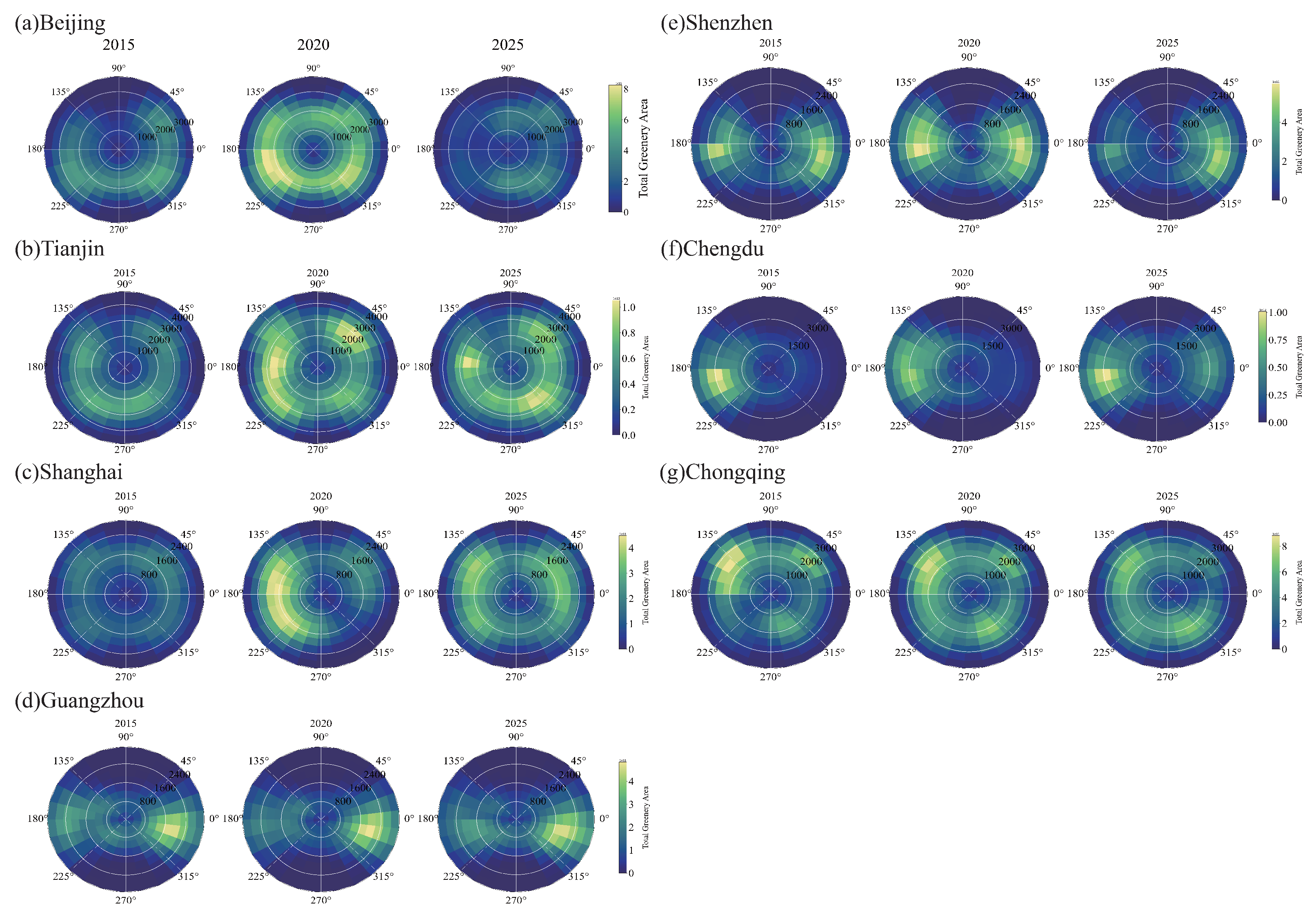
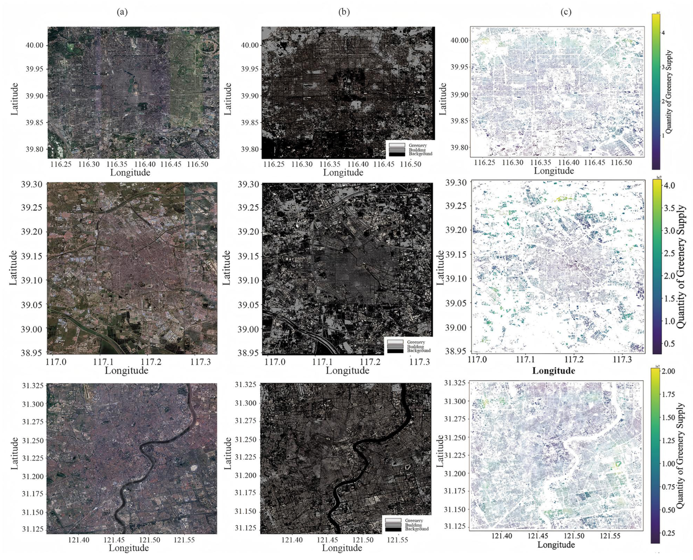
The nested-buffer method (see Appendix C) was used to characterise spatial variation in the green-space provision index within the urban morphological context (Figure 3). The maps for Beijing, Tianjin, and Shanghai in 2020 reveal distinct inter-city differences in the spatial distribution of green-space provision, providing the spatial context for the three-snapshot comparison presented in

Table 3. Temporal trends based on Sen’s slope estimates for the Gini coefficient, cumulative green-space provision index, and total building pixels.

Area	Indicator	Trend	Sen’s Slope
Beijing	Gini Coefficient	↑	$5.61\times {10}^{-3}$
	Cumulative Green-Space Provision Index	↓	$-7.19\times {10}^{11}$
	Total Building Pixels	↑	$4.75\times {10}^3$
Tianjin	Gini Coefficient	↓	$-3.33\times {10}^{-3}$
	Cumulative Green-Space Provision Index	↑	$3.42\times {10}^{12}$
	Total Building Pixels	↑	$6.79\times {10}^4$
Shanghai	Gini Coefficient	↓	$-1.60\times {10}^{-3}$
	Cumulative Green-Space Provision Index	↑	$1.64\times {10}^{12}$
	Total Building Pixels	↓	$-1.87\times {10}^4$
Guangzhou	Gini Coefficient	↑	$1.15\times {10}^{-3}$
	Cumulative Green-Space Provision Index	↓	$-1.67\times {10}^{11}$
	Total Building Pixels	↑	$2.29\times {10}^4$
Shenzhen	Gini Coefficient	↑	$1.47\times {10}^{-3}$
	Cumulative Green-Space Provision Index	↓	$-6.27\times {10}^{11}$
	Total Building Pixels	↓	$-2.62\times {10}^4$
Chengdu	Gini Coefficient	↓	$-5.50\times {10}^{-3}$
	Cumulative Green-Space Provision Index	↑	$1.25\times {10}^{12}$
	Total Building Pixels	↑	$6.27\times {10}^4$
Chongqing	Gini Coefficient	↑	$3.29\times {10}^{-4}$
	Cumulative Green-Space Provision Index	↑	$7.05\times {10}^9$
	Total Building Pixels	↑	$1.65\times {10}^4$

. Building upon these spatial patterns, Sen’s slope was used to describe the directional changes in the Gini coefficient, cumulative green-space provision index, and total building pixels between 2015 and 2025, which were derived from the city-level summary statistics reported in Appendix D. The results show that the direction and magnitude of change differed considerably among cities. Beijing and Shenzhen exhibited increasing Gini coefficients, with Beijing recording the largest positive Sen slope ($5.61\times {10}^{-3}$), whereas Chengdu showed the strongest negative slope ($-5.50\times {10}^{-3}$), suggesting an overall improvement in the spatial equity of green-space provision across the three observation years. Similar spatial heterogeneity was observed for the green-space provision index. Tianjin recorded the largest positive slope ($3.42\times {10}^{12}$), while Beijing showed the largest negative slope ($-7.19\times {10}^{11}$). Considering these changes, together with variations in total building pixels, reveals four broad descriptive pathways. Tianjin, Chengdu, and Chongqing experienced simultaneous increases in both the cumulative green-space provision index and total building pixels, whereas Beijing and Guangzhou showed declining green-space provision despite continued growth in total building pixels. In contrast, Shenzhen exhibited concurrent declines in both indicators, while Shanghai showed an increasing cumulative green-space provision index despite a reduction in total building pixels.

In terms of the evolution of spatial patterns, the distribution of QGS across cities between 2015 and 2025 exhibited substantial variation. Beijing and Tianjin demonstrated stable positive correlations (

Table 4. Evolution of Pearson correlation between green coverage and distance from the city centre in the core areas of seven megacities from 2015 to 2025.

City	Pearson Correlation Coefficient (r)	p-Value
Beijing	0.63	$8.5\times {10}^{-7}$
Tianjin	0.69	$3.1\times {10}^{-8}$
Shanghai	0.27	$5.5\times {10}^{-2}$
Guangzhou	$-0.86$	$5.8\times {10}^{-16}$
Shenzhen	$-0.89$	$4.0\times {10}^{-18}$
Chengdu	0.21	$1.4\times {10}^{-1}$
Chongqing	0.26	$6.9\times {10}^{-2}$

), with Pearson coefficients of 0.63 and 0.69, respectively ($p<0.001$). These cities generally followed an evolutionary path characterised by constrained central areas and outward expansion, where high-percentile green spaces extended towards peripheral zones while low-value central structures remained relatively stable, as summarised in

Table 5. Morphological evolution and quantile characteristics of green-space supply in China’s megacities.

City	Dynamic Characteristics of Spatial Distribution From 2015 to 2025 (Quantile Levels 1–6)
Beijing	Stable cold spots in the centre with outward expansion of peripheral hotspots: (1) Central areas have long been dominated by Level 1–2 (low-percentile) cold spots. (2) Level 5–6 (high-percentile) hotspots have progressively expanded towards peripheral areas and gradually formed more continuous spatial patterns.
Tianjin	Peripheral clustering of hotspots: (1) High-value patches are primarily concentrated along the northwestern and eastern edges of the study area. (2) The spatial configuration has gradually shifted from fragmented and dispersed distributions towards more continuous edge-based patches.
Shanghai	Middle-ring infilling and semi-circular enrichment: (1) High-percentile (Level 5–6) patches are mainly distributed within intermediate zones located at a certain distance from the urban centre. (2) The spatial evolution process exhibits a transition from fragmented distributions towards increasingly connected ring-like structures, accompanied by a gradual increase in hotspot proportion.
Guangzhou	Core concentration with pronounced radial attenuation: (1) Level 6 hotspots are densely concentrated around the urban core, exhibiting relatively strong spatial stability and increasing aggregation intensity over time. (2) Quantile values decline markedly with increasing distance from the city centre, forming a pronounced radial gradient.
Shenzhen	Persistent functional hubs within central and southern regions: (1) High-ranking hubs remain concentrated within the core areas of the central and southern regions, displaying relatively stable spatial characteristics. (2) Peripheral areas have long been characterised by lower-ranking fluctuations, whereas spatial resources remain strongly concentrated within the urban core.
Chengdu	Quadrant-oriented enrichment and transition towards ring-shaped structures: (1) High-percentile patches form a belt-like enrichment zone within the ${180}^{°}$–${270}^{°}$ quadrant. (2) Over time, the spatial distribution has gradually evolved from scattered patches towards a more evident ring-shaped configuration within the central section.
Chongqing	Clustered distribution with localised expansion: (1) High-percentile zones exhibit staggered distributions associated with urban clusters, without forming a clearly defined concentric-ring structure. (2) Under the influence of topographic constraints, high-value zones display patterns of localised dispersion accompanied by gradual spatial optimisation.

and illustrated by the spatial quantile clustering results. In contrast, Shenzhen and Guangzhou exhibited significant clustering characteristics ($p<0.001$), with green-space resources highly concentrated within core urban areas and declining rapidly with distance [60,61]. Their core hotspots intensified over time, indicating high spatial stability. Meanwhile, Shanghai, Chengdu, and Chongqing did not exhibit significant linear correlations ($p>0.05$). Their green-space distributions displayed pronounced non-linear characteristics, with high-value areas primarily concentrated within intermediate zones and transitioning from discrete to connected configurations. Among these, Chongqing presented a more complex clustered pattern potentially associated with topographic constraints [62].

Overall, between 2015 and 2025, the selected cities exhibited clear differences in green-space amount, equity evolution, and spatial distribution structures. These differences were reflected in divergent trajectories of green-space expansion and decline, varying trends in equity change, and the gradual transition of spatial structures from predominantly monocentric diffusion patterns towards the coexistence of concentric and clustered spatial configurations.

4.2. Nonlinear Associations Between Urban-Form Indicators and the Cumulative Green-Space Provision Index

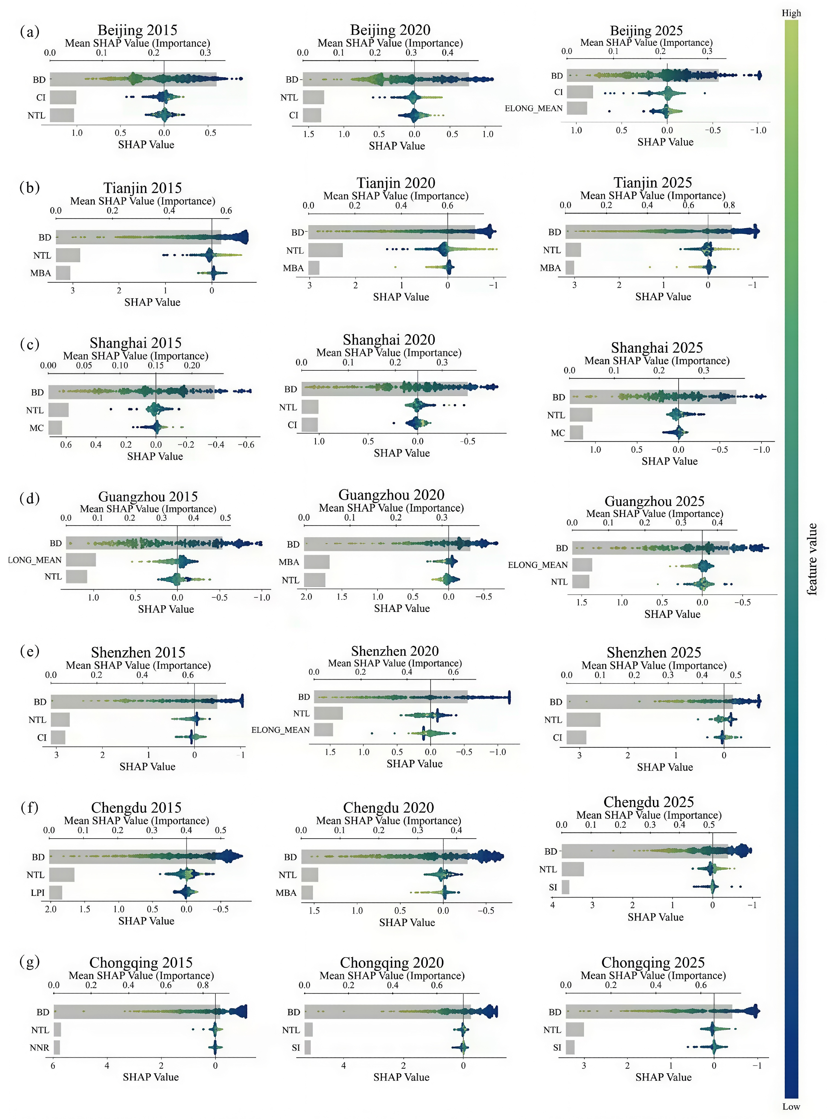
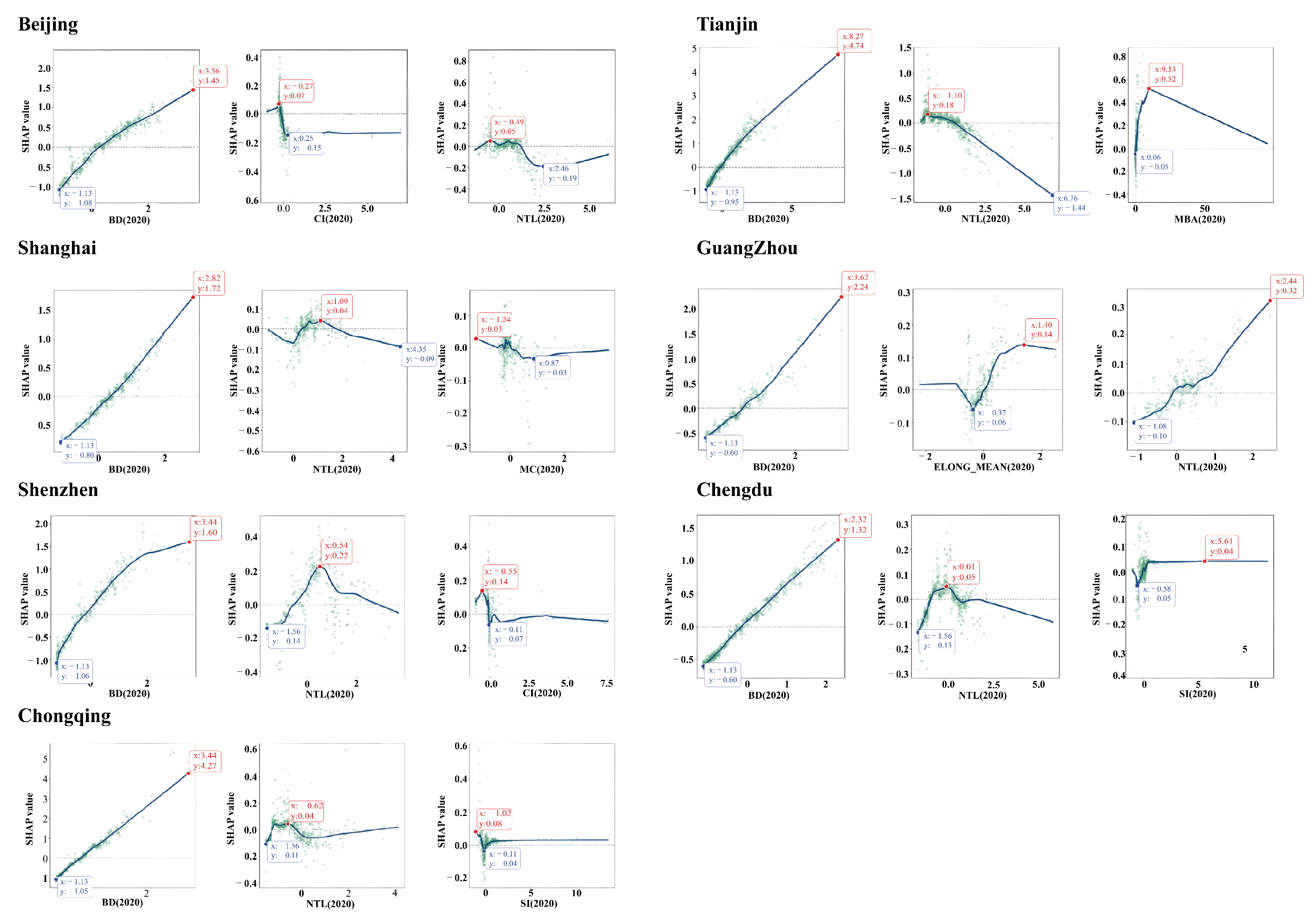
To systematically quantify the feature importance (Figure 4) and marginal effects (Figure 5) of urban-form indicators on green space, the Variance Inflation Factor (VIF) test was first employed to verify the absence of significant multicollinearity among the explanatory variables. As all VIF values remained below the critical threshold of 10, the essential modelling prerequisites were satisfied. Subsequently, the analysis was conducted using the XGBoost ensemble learning algorithm in conjunction with SHAP values. Due to space constraints and to avoid visual redundancy, the dominant response characteristics derived from the SHAP dependence plots are summarised in

Table 6. Summary of SHAP dependence patterns for major urban morphological indicators across the seven megacities.

Indicator	Overall Response	Consistency	Threshold	Dominant SHAP Response Pattern
BD	Positive	High	Weak saturation	Monotonic increase
MND	Negative	High	Saturation	Rapid decrease → stabilisation
CI	Non-linear	Medium	City-dependent	Weak turning point
MBA	Mixed	Low	Unstable	Positive/negative responses
ELONG_MEAN	Positive/Mixed	Medium	Unstable	Increasing in clustered cities
AD	Weak positive	Medium	No stable threshold	Gradual increase
AE_CV	Positive	Medium	No stable threshold	Continuous increase
LPI	Negative	Medium	Weak	Overall decreasing
NTL	Weak non-linear	Low	City-dependent	Weak heterogeneous response
SHDI	Weak	High	No threshold	Near-zero contribution

. The comprehensive analytical results, encompassing the models’ performance metrics and relative feature importance, are detailed in Appendix E. The resulting visualisations display the ranking of feature importance on the left, while the right side illustrates the distribution of variable contributions to the model’s predicted values. By examining the non-linear trends of these key indicators, this study characterises the complex associations between morphological factors and green-space provision in high-density environments, offering a quantitative framework for understanding patterns of spatial differentiation [63,64].

The results indicate that building density (BD) was generally the dominant predictor of spatial variation in green-space provision within megacity cores [65]; however, its influence pathways and non-linear response characteristics vary considerably among cities. In Beijing and Tianjin, BD exhibits a relatively strong positive association in both cases. In Beijing, the clumping index (CI) displays a threshold-like pattern characterised by an initial positive association followed by a suppressive effect at higher values, while the importance of night-time light (NTL) increased notably by 2025. In Tianjin, BD and NTL exhibit a pattern of joint influence, with mean building area (MBA) becoming increasingly important during later stages. In Guangzhou and Shenzhen, BD demonstrates a strong positive relationship and remains the dominant factor shaping spatial patterns. In Guangzhou, the positive contributions of the mean elongation index (ELONG_MEAN) and NTL gradually strengthen over time, whereas in Shenzhen, the clumping index (CI) shifts from a short-term positive association within low-value ranges to a more inhibitory pattern at higher levels. In Shanghai, Chengdu, and Chongqing, although BD continues to play a dominant role, NTL exhibits more complex non-linear characteristics, including fluctuating patterns of decrease followed by increase or increase followed by decrease in Shanghai, as well as increase-to-decrease trends in Chengdu and Chongqing. Meanwhile, the influence of morphological indicators such as morphological compactness (MC) and the shape index (SI) in these cities tends to weaken or remain relatively stable over time. Overall, although BD remains the dominant predictor, the association patterns across cities reflect multidimensional interactions among physical structure, functional vitality, and morphological characteristics.

In summary, the quantitative modelling results indicate that building density (BD) exhibits the highest feature contribution across all sample cities and serves as the primary variable associated with the spatial differentiation of green space. The results further suggest that the effects of different indicators on green space generally display pronounced non-linear characteristics, with the clumping index (CI) and night-time light (NTL) exhibiting substantial fluctuations in effect magnitude and threshold variation across different value ranges. Across the 2015, 2020, and 2025 snapshots, the rankings of indicator importance and the SHAP dependence patterns differed, indicating temporal variation in model-derived morphology–provision associations within megacity cores.

4.3. Statistical Identification and Clustering Classification of Green-Space Evolution Patterns

From the perspective of individual urban evolutionary trajectories and spatial structures, the distribution of green space exhibits distinct city-specific characteristics, and the associated driving mechanisms vary considerably among cities. Building upon the analysis of intra-city characteristics, extending the analysis to the full sample further clarifies the statistical distribution patterns of morphological factors at the inter-city level. Specifically, a Kruskal–Wallis non-parametric test was conducted across the three identified morphological clusters using the full sample of 21 city-year observations to evaluate intergroup distributional differences (

Table 7. Kruskal–Wallis test results for urban morphological indicators ($N=21$ city-year observations).

Indicator	H-Statistic	p-Value
AD	14.1818	0.0008
SI	14.7357	0.0006
BD	10.6448	0.0049
MBA	15.8364	0.0004
MND	13.3429	0.0013
NNR	7.9818	0.0185
CI	4.9721	0.0832
AE_CV	11.0714	0.0039
ELONG_MEAN	9.6221	0.0081
LPI	14.8214	0.0006
MC	9.4656	0.0088
SHDI	12.6318	0.0018
NTL	4.4782	0.1066

). According to the results, the MBA, SI, LPI, and AD indicators all exhibit highly significant intergroup differentiation across both spatial and temporal dimensions ($p<0.001$). Among these variables, the mean building area (MBA) presents the highest H-statistic ($15.8364$) among all morphological indicators, indicating the strongest spatial heterogeneity. At the same time, indicators such as BD, SHDI, and AE_CV also passed the significance test, suggesting substantial variation in their distributions across groups. In contrast, the p-value for night-time light (NTL) was $0.1066$, not reaching the significance threshold of $0.05$. This suggests that cities display a certain degree of similarity in NTL, with comparatively lower spatial heterogeneity than physical form indicators.

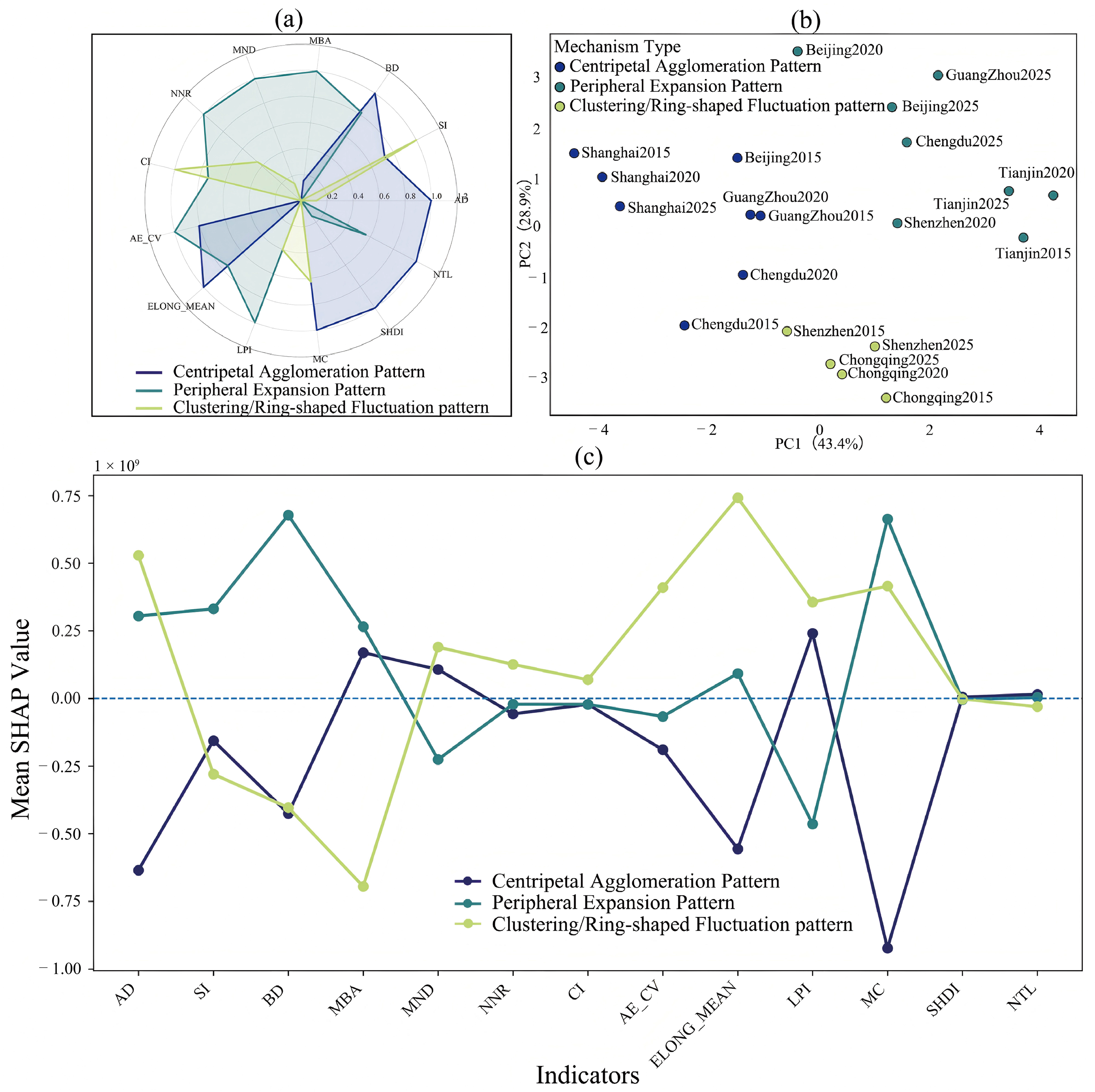
Based on PCA and K-means clustering (see Appendix F), the 21 city–year observations were classified into three representative morphology-related response patterns (

Table 8. Clustering results of urban morphological evolution patterns in megacity cores.

Morphology-Related Response Pattern	${\mathit{R}}^2$
Centripetal Agglomeration Pattern	0.4507
Peripheral Expansion Pattern	0.5099
Clustering/Ring-shaped Fluctuation Pattern	0.6403

), the characteristics of which are illustrated in the radar chart and PCA scatter plot (Figure 6). The Centripetal Agglomeration Pattern is characterised by relatively high values across multiple indicators, particularly MC, AD, BD, NTL, SHDI, and ELONG_MEAN. The Peripheral Expansion Pattern exhibits a comparatively balanced distribution of indicators while showing relatively stronger performance in MBA, MND, NNR, AE_CV, and LPI. The Clustering/Ring-shaped Fluctuation Pattern displays more pronounced directional characteristics and is primarily associated with the SI and CI. Further analysis indicates that the explanatory performance of the corresponding models increases progressively across the three mechanism types ($R^2$: $0.4507$, $0.5099$, and $0.6403$) and that most cities experienced cross-type transitions between 2015 and 2025. Meanwhile, the cluster boundaries within the PCA space remain relatively distinct, further highlighting the heterogeneity of morphological evolution pathways among different cities.

To compare the predictive contributions of urban morphological indicators among the three clusters, we calculated the mean SHAP value of each indicator within each cluster. Distinct contribution profiles were observed across the three morphology-related response patterns (Figure 6). Distinct contribution patterns were observed across the three mechanisms. In the Centripetal Agglomeration Pattern, building density (BD), mean building area (MBA), mean nearest distance (MND), and the largest patch index (LPI) exhibited positive contributions to the model prediction, whereas the average distance (AD), building shape index (SI), mean elongation index (ELONG_MEAN), and morphological compactness (MC) showed negative contributions. Among these variables, MC produced the largest negative mean SHAP value (approximately $-0.92\times {10}^9$), indicating that a higher MC was associated with lower predicted green-space provision under highly compact urban configurations. By contrast, the Peripheral Expansion Pattern was characterised by the strongest positive contribution from BD (approximately $+0.68\times {10}^9$), followed by MC and SI, whereas LPI and MND exhibited comparatively strong negative contributions and the remaining indicators were generally distributed close to zero, suggesting relatively limited predictive influence. The Clustering/Ring-shaped Fluctuation Pattern displayed a different contribution structure, in which ELONG_MEAN produced the largest positive contribution (approximately $+0.74\times {10}^9$), followed by AD, AE_CV, MC, and MND, while MBA and SI showed the strongest negative contributions (approximately $-0.70\times {10}^9$ and $-0.28\times {10}^9$, respectively), indicating substantial heterogeneity in the predictive roles of urban morphological indicators across evolutionary mechanisms. These mechanism-level differences are further supported by the SHAP dependence plots for the seven cities. Across cities, BD consistently exhibited an approximately monotonic positive relationship with the predicted green-space provision index, whereas MND generally showed a rapid decline followed by gradual stabilisation, indicating diminishing marginal effects. CI and NTL displayed comparatively heterogeneous and nonlinear response patterns, while MBA and ELONG_MEAN varied substantially among different urban contexts. By contrast, SHDI remained close to zero in most city-year models, suggesting a consistently limited contribution to model prediction.

Across all three mechanism types, SHDI and NTL remained consistently close to zero, indicating comparatively stable and limited contributions to the model prediction. Overall, both the magnitude and direction of the SHAP contributions varied considerably among the three morphological mechanisms, suggesting that the relationships between urban morphology and the green-space provision index are strongly context-dependent. It should be emphasised that the reported SHAP values represent model-derived predictive contributions rather than evidence of causal relationships, and the interpretation of the contribution direction is therefore limited to the fitted XGBoost model. In addition, potential threshold effects of key indicators were assessed using SHAP dependence plots. Consistent threshold behaviour was observed only for a limited number of indicators, whereas most response curves exhibited either monotonic trends or city-specific non-linear responses. Threshold values are reported only where robust inflection points could be identified from the SHAP dependence curves; otherwise, indicators were classified as exhibiting unstable or non-threshold responses. Consequently, the reported threshold ranges should be interpreted as model-specific characteristics rather than universal ecological thresholds.

5. Discussion

5.1. Planning Responses to Spatial–Temporal Variations in Green Spaces

The findings indicate that associations between urban morphology and green-space provision vary substantially across urban-development stages, spatial structures, and development intensities. The traditional green-space allocation model based on homogeneous incremental growth may no longer adequately respond to the practical demands of contemporary urban development. Accordingly, future urban ecological governance may benefit from a gradual shift of its focus from scale expansion towards structural optimisation and targeted regulation, particularly under conditions of land scarcity and increasing ecological demand [66,67]. Through differentiated governance strategies based on urban morphological characteristics, it may be possible to enhance both ecological performance and spatial equity under conditions of limited spatial resources [68]. Specifically, the Centripetal Agglomeration Pattern, which is largely associated with spatial compression under conditions of high density and compactness, may require improvements in ecological embedding capacity within highly developed built environments through the fragmentation of continuous high-intensity interfaces, the release of ecological permeability corridors, and the expansion of three-dimensional ecological spaces such as rooftop and vertical greening. The Peripheral Expansion Pattern, by contrast, is more frequently associated with lagging green-space provision and fragmented green patches. In this context, embedded ecological remediation and network reconstruction through pocket parks, street-corner green spaces, and ecological corridors may help improve spatial connectivity, while stronger ecological constraints during early-stage development may reduce the need for costly post-development interventions. The Clustering/Ring-shaped Fluctuation Pattern is characterised by relatively insufficient coordination of green-space provision within multi-centred urban structures. Governance priorities in these areas may therefore focus on strengthening ecological connectivity and functional integration among clusters, constructing regional green networks through transport and open-space systems, and promoting the transformation of green spaces into multifunctional systems integrating ecological, recreational, and disaster-prevention functions. Overall, although optimisation pathways differ among mechanism types, their common direction involves a transition from incremental expansion towards structural optimisation and mechanism-oriented regulation. This transition may facilitate the coordinated improvement of green-space equity and ecological efficiency through spatial restructuring, ecological network optimisation, and functional reorganisation within high-density built environments [69,70].

5.2. Temporal Variation and Nonlinear Patterns of Morphology–Provision Associations

The three-snapshot analysis suggests that the model-derived relationships between urban morphology and the spatial equity of green-space provision varied systematically across cities and observation years. In the earlier observation years, green-space equity was more strongly associated with physical morphology indicators, including building density and compactness, which may reflect the spatial constraints imposed by high-intensity urban development. In the later snapshots, indicators related to urban vitality, including night-time lighting and functional mix, showed higher relative importance in several models [71,72]. Together, these patterns suggest a possible shift from a space-supply perspective toward a more demand-responsive interpretation of green-space provision. However, because the present analysis does not include direct observations of residents’ use behaviour, socioeconomic characteristics, housing prices, or planning policy, these findings should be interpreted as evidence of morphology-based statistical associations rather than definitive evidence of the mechanisms underlying green-space equity.

The SHAP dependence analysis further demonstrated that the relationships between urban morphological indicators and the green-space provision index were predominantly nonlinear and strongly context-dependent. Rather than exhibiting universal threshold values, most indicators showed gradual changes in marginal contributions across their observed ranges. Building density (BD) consistently displayed a positive response in nearly all city-year models, although the increasing trend generally became weaker at higher values, indicating diminishing marginal gains. By contrast, mean nearest distance (MND) exhibited a rapid decline followed by gradual stabilisation, suggesting that its marginal influence became progressively weaker once spatial dispersion exceeded a certain level. Indicators describing urban configuration, including the clumping index (CI), mean elongation index (ELONG_MEAN), and mean building area (MBA), showed substantial heterogeneity among cities, reflecting the influences of different urban development pathways and morphological contexts. In comparison, SHDI and night-time light (NTL) remained relatively stable, with consistently small SHAP values, indicating comparatively limited predictive contributions across different urban environments.

These findings suggest that the relationships identified by the XGBoost–SHAP framework should be interpreted as model-derived response patterns rather than evidence of universal ecological thresholds or causal mechanisms. Although several indicators exhibited local turning behaviour in individual cities, the locations of these inflection points were not sufficiently consistent across the seven megacities to justify the definition of fixed planning thresholds. Consequently, urban morphological indicators are more appropriately regarded as diagnostic variables for the identification of areas with relatively high or low green-space provision potential rather than prescriptive planning criteria. Therefore, practical planning decisions should integrate additional information, including socioeconomic demand, accessibility to green spaces, and observed human activity patterns, to support context-specific urban greening strategies [73].

5.3. Implications for Urban Management and Limitations of the Study Based on the Classification of Green Space

By integrating high-resolution remote-sensing data with interpretable machine-learning methods, this study systematically examines model-derived associations between multidimensional urban morphology and green-space provision within the core areas of Chinese megacities. An analytical framework encompassing morphology, mechanism, and classification was constructed, providing quantitative support for ecological space optimisation and cross-city comparative analysis during the stage of stock-oriented urban development [74,75]. The findings suggest that green-space equity in high-density cities is associated not only with physical spatial structures but also with functional organisation, human activities, and the evolution of urban development patterns. This further indicates that future urban ecological governance may need to gradually shift from an emphasis on incremental green-space supply towards a more comprehensive governance framework focused on structural optimisation and dynamic regulation.

Several limitations should be considered when interpreting these findings. Although the proposed framework comprehensively quantified urban morphology and green-space provision, it primarily focused on the physical environment and did not explicitly incorporate socioeconomic determinants such as population density, income inequality, demographic structure, housing prices, planning policy, or residents’ actual use behaviour. Consequently, the results should be interpreted as reflecting the spatial configuration of green-space provision rather than the broader social dimension of environmental justice [76]. In addition, the nested-buffer approach is based on Euclidean distance and therefore cannot fully represent realised accessibility through street networks, pedestrian barriers, or terrain conditions. The temporal analysis relied on three representative years (2015, 2020, and 2025), providing snapshots of urban evolution rather than continuous long-term trajectories, while historical Google Earth imagery may introduce uncertainty due to differences in acquisition date, sensor characteristics, seasonal conditions, and radiometric consistency across cities and years. Furthermore, the XGBoost–SHAP framework identifies model-derived predictive associations rather than causal relationships, and the interpretation of SHAP values depends on model performance, particularly for city-year models with relatively low predictive accuracy. Therefore, future research should integrate longer time-series observations, network-based accessibility measures, socioeconomic and behavioural variables, and causal inference approaches to improve the robustness and generalisability of urban green-space equity assessment [77].

6. Conclusions

This study investigated the spatial equity of green-space provision across the core areas of seven Chinese megacities using high-resolution remote-sensing data acquired in 2015, 2020, and 2025. By integrating PSPNet-based semantic segmentation, nested-buffer measurement, the Gini coefficient, XGBoost-SHAP analysis, and spatial typology classification, a unified analytical framework was established to reveal the relationships between urban morphology and the spatial differentiation of green-space provision. Rather than focusing solely on the quantity of green space, this framework explicitly incorporates spatial distribution and equity, providing a morphology-oriented perspective for the evaluation of green-space provision under high-density urban development.

The results demonstrate that changes in the green-space provision index and its spatial inequality were not synchronised across the seven megacities, highlighting pronounced spatial heterogeneity in their evolutionary trajectories. Building density consistently contributed most strongly in most city-year models, whereas compactness-related indicators showed nonlinear, city-specific response patterns. Comparative analysis further identified three representative morphology-related response patterns: the Centripetal Agglomeration Pattern, Peripheral Expansion Pattern, and Clustering/Ring-shaped Fluctuation Pattern. These patterns reveal that the morpho-green relationship is highly context-dependent and cannot be addressed through a one-size-fits-all strategy; instead, differentiated governance must align with each city’s dominant evolutionary mechanism. Ultimately, improving green-space equity in high-density cities requires not just expansion of the quantity of green spaces but optimisation of spatial configurations tailored to specific urban morphological contexts.

Overall, this study provides a transferable analytical framework linking urban morphology with the spatial equity of green-space provision and offers quantitative evidence to support morphology-informed ecological planning in high-density megacities. Because the reported SHAP values represent model-based predictive associations rather than causal relationships, the findings should primarily be interpreted as identifying priority areas for spatial optimisation rather than prescribing fixed planning thresholds. Future research should integrate longer temporal records, network-based accessibility, socioeconomic characteristics, and observed green-space use to further improve the understanding of green-space justice and support evidence-based urban ecological governance.

References

1. Seto, K.C.; Güneralp, B.; Hutyra, L.R. Global forecasts of urban expansion to 2030 and direct impacts on biodiversity and carbon pools. Proc. Natl. Acad. Sci. USA 2012, 109, 16083–16088. [Google Scholar] [CrossRef] [PubMed]
2. Wu, J. Urban ecology and sustainability: The state-of-the-science and future directions. Landsc. Urban Plan. 2014, 125, 209–221. [Google Scholar] [CrossRef]
3. Haase, D.; Frantzeskaki, N.; Elmqvist, T. Ecosystem Services in Urban Landscapes: Practical Applications and Governance Implications. AMBIO 2014, 43, 407–412. [Google Scholar] [CrossRef] [PubMed]
4. Wolch, J.R.; Byrne, J.; Newell, J.P. Urban green space, public health, and environmental justice: The challenge of making cities ‘just green enough’. Landsc. Urban Plan. 2014, 125, 234–244. [Google Scholar] [CrossRef]
5. Rigolon, A. A complex landscape of inequity in access to urban parks: A literature review. Landsc. Urban Plan. 2016, 153, 160–169. [Google Scholar] [CrossRef]
6. Dai, D. Racial/ethnic and socioeconomic disparities in urban green space accessibility: Where to intervene? Landsc. Urban Plan. 2011, 102, 234–244. [Google Scholar] [CrossRef]
7. Haaland, C.; van den Bosch, C.K. Challenges and strategies for urban green-space planning in cities undergoing densification: A review. Urban For. Urban Green. 2015, 14, 760–771. [Google Scholar] [CrossRef]
8. Chen, J.; Kinoshita, T.; Li, H.; Luo, S.; Su, D.; Yang, X.; Hu, Y. Toward green equity: An extensive study on urban form and green space equity for shrinking cities. Sustain. Cities Soc. 2023, 90, 104395. [Google Scholar] [CrossRef]
9. Schwarz, N. Urban form revisited—Selecting indicators for characterising European cities. Landsc. Urban Plan. 2010, 96, 29–47. [Google Scholar] [CrossRef]
10. Zhu, Z.; Li, J.; Chen, Z. Green space equity: Spatial distribution of urban green spaces and correlation with urbanization in Xiamen, China. Environ. Dev. Sustain. 2022, 25, 423–443. [Google Scholar] [CrossRef]
11. Luo, H.; Zhou, R.; Li, C.; Ma, Q.; Fang, X.; Hu, Y.; Lv, X.; Dong, Z.; Tian, Y.; Fang, S. Quantifying the nonlinear interactions of 2D/3D building and green space morphology on land surface temperature across different urban functional zones. Sustain. Cities Soc. 2026, 138, 107175. [Google Scholar] [CrossRef]
12. Chen, J.; Kinoshita, T.; Li, H.; Luo, S.; Su, D. Which green is more equitable? A study of urban green space equity based on morphological spatial patterns. Urban For. Urban Green. 2024, 91, 128178. [Google Scholar] [CrossRef]
13. Shen, J.; Fan, J.; Wu, S.; Xu, X.; Fei, Y.; Liu, Z.; Xiong, S. A Study on the Impact of a Community Green Space Built Environment on Physical Activity in Older People from a Health Perspective: A Case Study of Qingshan District, Wuhan. Sustainability 2025, 17, 263. [Google Scholar] [CrossRef]
14. Hu, L.; Zhou, X.; Ruan, J.; Li, S. ASPP+-LANet: A Multi-Scale Context Extraction Network for Semantic Segmentation of High-Resolution Remote Sensing Images. Remote Sens. 2024, 16, 1036. [Google Scholar] [CrossRef]
15. Wang, Z.; Zhou, R.; Yu, Y. The impact of urban morphology on land surface temperature under seasonal and diurnal variations: Marginal and interaction effects. Build. Environ. 2025, 272, 112673. [Google Scholar] [CrossRef]
16. Tzoulas, K.; Korpela, K.; Venn, S.; Yli-Pelkonen, V.; Kaźmierczak, A.; Niemela, J.; James, P. Promoting ecosystem and human health in urban areas using Green Infrastructure: A literature review. Landsc. Urban Plan. 2007, 81, 167–178. [Google Scholar] [CrossRef]
17. Gill, S.; Handley, J.; Ennos, A.; Pauleit, S. Adapting Cities for Climate Change: The Role of the Green Infrastructure. Built Environ. 2007, 33, 115–133. [Google Scholar] [CrossRef]
18. Cao, Y.; Li, G.; Huang, Y. Spatiotemporal Evolution of Residential Exposure to Green Space in Beijing. Remote Sens. 2023, 15, 1549. [Google Scholar] [CrossRef]
19. Zhao, Y.; Tang, X.; Liao, Z.; Liu, Y.; Liu, M.; Lin, J. Multi-Type Features Embedded Deep Learning Framework for Residential Building Prediction. ISPRS Int. J. Geo-Inf. 2023, 12, 356. [Google Scholar] [CrossRef]
20. Wu, J.; Li, C. Illustrating the nonlinear effects of urban form factors on transportation carbon emissions based on gradient boosting decision trees. Sci. Total Environ. 2024, 929, 172547. [Google Scholar] [CrossRef] [PubMed]
21. Liu, W.; Yang, Z.; Gui, C.; Li, G.; Xu, H. Investigating the Nonlinear Relationship Between the Built Environment and Urban Vitality Based on Multi-Source Data and Interpretable Machine Learning. Buildings 2025, 15, 1414. [Google Scholar] [CrossRef]
22. Fang, X.; Ma, Q.; Wu, L.; Liu, X. Distributional environmental justice of residential walking space: The lens of urban ecosystem services supply and demand. J. Environ. Manag. 2023, 329, 117050. [Google Scholar] [CrossRef] [PubMed]
23. Wang, S.; Jia, M.; Zhou, Y.; Fan, F. Impacts of changing urban form on ecological efficiency in China: A comparison between urban agglomerations and administrative areas. J. Environ. Plan. Manag. 2019, 63, 1834–1856. [Google Scholar] [CrossRef]
24. Kang, C.D. Nonlinear and spatial effects of urban form on building electricity consumption in Seoul, South Korea: Urban morphometric and XGBoost approaches. Cities 2026, 170, 106624. [Google Scholar] [CrossRef]
25. Seto, K.C.; Fragkias, M.; Güneralp, B.; Reilly, M.K. A Meta-Analysis of Global Urban Land Expansion. PLoS ONE 2011, 6, e23777. [Google Scholar] [CrossRef] [PubMed]
26. Hu, Y.; Connor, D.S.; Stuhlmacher, M.; Peng, J.; Turner, B.L., II. More urbanization, more polarization: Evidence from two decades of urban expansion in China. npj Urban Sustain. 2024, 4, 33. [Google Scholar] [CrossRef]
27. Kuang, W. Mapping global impervious surface area and green space within urban environments. Sci. China Earth Sci. 2019, 62, 1591–1606. [Google Scholar] [CrossRef]
28. Chen, T.; Guestrin, C. XGBoost: A Scalable Tree Boosting System. In Proceedings of the 22nd ACM SIGKDD International Conference on Knowledge Discovery and Data Mining (KDD ’16), San Francisco, CA, USA, 13–17 August 2016; pp. 785–794. [Google Scholar] [CrossRef]
29. Rezaei, N.; Millard-Ball, A. Urban form and its impacts on air pollution and access to green space: A global analysis of 462 cities. PLoS ONE 2023, 18, e0278265. [Google Scholar] [CrossRef] [PubMed]
30. Huang, B.; Gu, J.; Zhang, M.; Feng, Z. Green Space Equality Is Better in Fast-Growing Cities: Evidence from 140 Cities in China. Land 2025, 14, 366. [Google Scholar] [CrossRef]
31. Yu, Z.; Ma, W.; Hu, J.; Yang, G.; Liu, H.; Zhou, Y.; Li, X.; Li, Y.; Guan, C.; Ma, W.; et al. Greening dominates greenspace exposure inequality in Chinese cities. npj Urban Sustain. 2025, 5, 73. [Google Scholar] [CrossRef]
32. Han, Y.; Oh, J. Automated Geo/Co-Registration of Multi-Temporal Very-High-Resolution Imagery. Sensors 2018, 18, 1599. [Google Scholar] [CrossRef] [PubMed]
33. Li, Y.; Li, P.; Wang, H.; Gong, X.; Fang, Z. CAML-PSPNet: A Medical Image Segmentation Network Based on Coordinate Attention and a Mixed Loss Function. Sensors 2025, 25, 1117. [Google Scholar] [CrossRef] [PubMed]
34. Yuan, X.; Shi, J.; Gu, L. A review of deep learning methods for semantic segmentation of remote sensing imagery. Expert Syst. Appl. 2021, 169, 114417. [Google Scholar] [CrossRef]
35. Wang, H.; Yu, F.; Xie, J.; Wang, H.; Zheng, H. Road Extraction Based on Improved Deeplabv3 Plus in Remote Sensing Image. Int. Arch. Photogramm. Remote Sens. Spat. Inf. Sci. 2022, XLVIII-3/W2-2022, 67–72. [Google Scholar] [CrossRef]
36. Papadomanolaki, M.; Vakalopoulou, M.; Karantzalos, K. A Novel Object-Based Deep Learning Framework for Semantic Segmentation of Very High-Resolution Remote Sensing Data: Comparison with Convolutional and Fully Convolutional Networks. Remote Sens. 2019, 11, 684. [Google Scholar] [CrossRef]
37. Zhang, J.; Yu, Z.; Cheng, Y.; Chen, C.; Wan, Y.; Zhao, B.; Vejre, H. Evaluating the disparities in urban green space provision in communities with diverse built environments: The case of a rapidly urbanizing Chinese city. Build. Environ. 2020, 183, 107170. [Google Scholar] [CrossRef]
38. Bizotto, F.; Giraldi, G.A.; Junior, J.M.; da Silva, V.P.; Imbelloni, A.C.; Andrade, M.L.; Marcatto, J.; Brito, A. Convolutional neural networks for semantic segmentation of aerial images in land cover mapping of environmental protection areas. Remote Sens. Appl. Soc. Environ. 2025, 40, 101707. [Google Scholar] [CrossRef]
39. Liu, J.; Wang, H.; Cheng, Y.; Sun, Y.; Yang, C. Urban park quality assessment: A synergy-differentiation approach integrating landscape, behavior and emotion. J. Clean. Prod. 2026, 543, 147633. [Google Scholar] [CrossRef]
40. Soni, T.K.; Pujari, P. Emerging deep learning approaches for urban satellite image analysis: A survey on classification, segmentation, and change detection. Evol. Intell. 2025, 18, 106. [Google Scholar] [CrossRef]
41. Zheng, B.; Tian, F.; Lin, L.; Fan, J. Study on the Morphological Analysis and Evolution of the Street Network in the Historic Urban Area of Changsha City from 1872–2023. Land 2024, 13, 738. [Google Scholar] [CrossRef]
42. Boeing, G. Street Network Models and Measures for Every U.S. City, County, Urbanized Area, Census Tract, and Zillow-Defined Neighborhood. Urban Sci. 2019, 3, 28. [Google Scholar] [CrossRef]
43. Ye, Y.; Zeng, W.; Shen, Q.; Zhang, X.; Lu, Y. The visual quality of streets: A human-centred continuous measurement based on machine learning algorithms and street view images. Environ. Plan. B Urban Anal. City Sci. 2019, 46, 1439–1457. [Google Scholar] [CrossRef]
44. Chen, J.; Liu, B.; Li, S.; Jiang, B.; Wang, X.; Lu, W.; Hu, Y.; Wen, T.; Feng, Y. Actual supply-demand of the urban green space in a populous and highly developed city: Evidence based on mobile signal data in Guangzhou. Ecol. Indic. 2024, 169, 112839. [Google Scholar] [CrossRef]
45. Rigolon, A.; Browning, M.H.E.M.; Lee, K.; Shin, S. Access to Urban Green Space in Cities of the Global South: A Systematic Literature Review. Urban Sci. 2018, 2, 67. [Google Scholar] [CrossRef]
46. Nesbitt, L.; Meitner, M.J.; Girling, C.; Sheppard, S.R.; Lu, Y. Who has access to urban vegetation? A spatial analysis of distributional green equity in 10 US cities. Landsc. Urban Plan. 2019, 181, 51–79. [Google Scholar] [CrossRef]
47. Cheng, P.; Min, M.; Hu, W.; Zhang, A. A Framework for Fairness Evaluation and Improvement of Urban Green Space: A Case of Wuhan Metropolitan Area in China. Forests 2021, 12, 890. [Google Scholar] [CrossRef]
48. Yang, G.; Zhao, Y.; Xing, H.; Fu, Y.; Liu, G.; Kang, X.; Mai, X. Understanding the changes in spatial fairness of urban greenery using time-series remote sensing images: A case study of Guangdong-Hong Kong-Macao Greater Bay. Sci. Total Environ. 2020, 715, 136763. [Google Scholar] [CrossRef] [PubMed]
49. Browning, M.; Lee, K. Within What Distance Does “Greenness” Best Predict Physical Health? A Systematic Review of Articles with GIS Buffer Analyses across the Lifespan. Int. J. Environ. Res. Public Health 2017, 14, 675. [Google Scholar] [CrossRef] [PubMed]
50. Garba, H.; Udokpoh, U.U. Analysis of Trend in Meteorological and Hydrological Time-series using Mann-Kendall and Sen’s Slope Estimator Statistical Test in Akwa Ibom State, Nigeria. Int. J. Environ. Clim. Change 2023, 13, 1017–1035. [Google Scholar] [CrossRef]
51. Yang, H.; Li, Y.; Zhang, L.; Mao, X.; Liu, X.; Yang, M.; Chang, Z.; Deng, J.; Yang, R. Spatiotemporal Evolution of Vegetation Cover and Identification of Driving Factors Based on kNDVI and XGBoost-SHAP: A Study from Qinghai Province, China. Land 2026, 15, 338. [Google Scholar] [CrossRef]
52. Ahmed Al-Azri, N.; Bello Danbatta, M.; Al-Saadi, S. Meteorological Forecasting in Oman: A Comparative Analysis of Artificial Neural Networks, Support Vector Machines, Random Forest and Extreme Gradient Boosting Using Long-Term Historical Data (1984–2024). J. Phys. Conf. Ser. 2026, 3191, 012048. [Google Scholar] [CrossRef]
53. Yang, X.; Liu, Z.; Chen, H.; Yang, L. Research on Gain Allocation Strategy of Multi-park Integrated Energy System Based on Cooperative Game and Improved Shapley Value Method. J. Electr. Eng. Technol. 2025, 21, 189–202. [Google Scholar] [CrossRef]
54. Lian, A.; Zhang, Y.; Cai, Y.; Wang, Z.; Sun, X.; Jiao, Y.; Dong, R. Exploring the nonlinear relationship and interaction effects between the built environment and street vitality using machine learning methods. Ecol. Front. 2026, 46, 932–946. [Google Scholar] [CrossRef]
55. Fryer, D.; Strumke, I.; Nguyen, H. Shapley Values for Feature Selection: The Good, the Bad, and the Axioms. IEEE Access 2021, 9, 144352–144360. [Google Scholar] [CrossRef]
56. Probst, P.; Wright, M.N.; Boulesteix, A. Hyperparameters and tuning strategies for random forest. Wires Data Min. Knowl. Discov. 2019, 9. [Google Scholar] [CrossRef]
57. Fan, N.; Zhang, L.; Liu, R. Cross-dimensional principal component analysis. Digit. Signal Process. 2026, 180, 106227. [Google Scholar] [CrossRef]
58. Zhang, Z.; Lan, J.; Zhang, Z. K-means clustering algorithm based on bee colony strategy. J. Phys. Conf. Ser. 2021, 2031, 012058. [Google Scholar] [CrossRef]
59. Yang, W.; Yang, R.; Zhou, S. The spatial heterogeneity of urban green space inequity from a perspective of the vulnerable: A case study of Guangzhou, China. Cities 2022, 130, 103855. [Google Scholar] [CrossRef]
60. Lian, Z.; Feng, X. Urban Green Space Pattern in Core Cities of the Greater Bay Area Based on Morphological Spatial Pattern Analysis. Sustainability 2022, 14, 12365. [Google Scholar] [CrossRef]
61. Ge, J.; Shi, Y. Dynamics of urban green spaces in a megacity under the green economy framework and their influencing factors: A case study of Chongqing urban area. Front. Public Health 2025, 12. [Google Scholar] [CrossRef] [PubMed]
62. Zhang, Z.; Wang, R.; Zhang, S.; Meng, W. Explainable machine learning reveals the nonlinear relationships between green innovation and coordinated urban-rural development: Evidence from the Yangtze River Delta urban agglomeration, China. Environ. Impact Assess. Rev. 2026, 118, 108320. [Google Scholar] [CrossRef]
63. Choi, H.W.; Jung, D.Y.; Kim, S.; Koo, J.R.; Heo, Y.; Song, S.W.; Kang, Y.T. A review on passive/active technologies towards plus energy building in high density urban area. Renew. Sustain. Energy Rev. 2026, 235, 116973. [Google Scholar] [CrossRef]
64. Haase, D.; Kabisch, S.; Haase, A.; Andersson, E.; Banzhaf, E.; Baró, F.; Brenck, M.; Fischer, L.K.; Frantzeskaki, N.; Kabisch, N.; et al. Greening cities—To be socially inclusive? About the alleged paradox of society and ecology in cities. Habitat Int. 2017, 64, 41–48. [Google Scholar] [CrossRef]
65. Kabisch, N.; van den Bosch, M.; Lafortezza, R. The health benefits of nature-based solutions to urbanization challenges for children and the elderly—A systematic review. Environ. Res. 2017, 159, 362–373. [Google Scholar] [CrossRef] [PubMed]
66. Ricci, L.; Mariano, C.; Marino, M. Rethinking Cities Beyond Climate Neutrality: Justice and Inclusion to Prevent Climate Gentrification. Appl. Sci. 2025, 16, 259. [Google Scholar] [CrossRef]
67. Dyer, G.M.; Khomenko, S.; Adlakha, D.; Anenberg, S.; Behnisch, M.; Boeing, G.; Esperon-Rodriguez, M.; Gasparrini, A.; Khreis, H.; Kondo, M.C.; et al. Exploring the nexus of urban form, transport, environment and health in large-scale urban studies: A state-of-the-art scoping review. Environ. Res. 2024, 257, 119324. [Google Scholar] [CrossRef] [PubMed]
68. Yang, Y.; Tang, S. Examining Residents’ Perceptions and Usage Preferences of Urban Public Green Spaces Through the Lens of Environmental Justice. Sustainability 2025, 17, 2627. [Google Scholar] [CrossRef]
69. Meerow, S.; Newell, J.P. Spatial planning for multifunctional green infrastructure: Growing resilience in Detroit. Landsc. Urban Plan. 2017, 159, 62–75. [Google Scholar] [CrossRef]
70. Jiaxin, S.; Jiansong, P. Park green space accessibility and equity for age-friendly urban living in Kunming’s central district. Sci. Rep. 2026, 16, 17162. [Google Scholar] [CrossRef] [PubMed]
71. Fan, P.; Ouyang, Z.; Basnou, C.; Pino, J.; Park, H.; Chen, J. Nature-based solutions for urban landscapes under post-industrialization and globalization: Barcelona versus Shanghai. Environ. Res. 2017, 156, 272–283. [Google Scholar] [CrossRef] [PubMed]
72. Zheng, H.; Wu, Y.; He, H.; Delang, C.O.; Lu, J.; Yao, Z.; Dong, S. Urbanization and urban energy eco-efficiency: A meta-frontier super EBM analysis based on 271 cities of China. Sustain. Cities Soc. 2024, 101, 105089. [Google Scholar] [CrossRef]
73. Zhang, H.; Smith, J.W. A data-driven and generalizable model for classifying outdoor recreation opportunities at multiple spatial extents. Landsc. Urban Plan. 2023, 240, 104876. [Google Scholar] [CrossRef]
74. Donati, F.; Rodríguez-García, M.J. Gender mainstreaming in urban projects: A measurement proposal applied to Spanish Urban regeneration policies. Cities 2024, 150, 105090. [Google Scholar] [CrossRef]
75. Jiang, Y.; Neisch, P.M.; Cui, T. Rethinking urban inequality through a behavioural lens: Informal public space activities (IPSAs) as diagnostic tools for behavioural equity and public space resilience in urban planning. Sustain. Cities Soc. 2026, 143, 107379. [Google Scholar] [CrossRef]
76. Dudek, T. Recreation in suburban forests – monitoring the distribution of visits using the example of Rzeszów. Ann. For. Res. 2024, 67, 131–141. [Google Scholar] [CrossRef]
77. Li, Z. Extracting spatial effects from machine learning model using local interpretation method: An example of SHAP and XGBoost. Comput. Environ. Urban Syst. 2022, 96, 101845. [Google Scholar] [CrossRef]
Figure 1. Core areas of seven Chinese megacities.
Forests 17 00874 g001
Figure 2. Research framework.
Forests 17 00874 g002
Figure 3. Spatial distribution of the green-space provision index across the selected megacity cores.
Forests 17 00874 g003
Figure 4. Relative importance and differences in the contributions of urban-form indicators.
Forests 17 00874 g004
Figure 5. SHAP dependence patterns for associations between urban-form indicators and green-space provision in megacity core areas.
Forests 17 00874 g005
Figure 6. (a) Multi-dimensional morphological indicator distributions across clustered mechanisms; (b) PCA-based clustering distribution of urban morphological evolution patterns; (c) comparison of average marginal effects across different mechanism zones.
Forests 17 00874 g006