Estimating Aboveground Biomass and Surface Fuels in Semi-Arid Oak–Pine Forests Using Sentinel-2 Spectral Indices and Gamma GLMs

Abstract

Estimation of forest biomass and surface fuels is essential for wildfire risk assessment, carbon accounting, and ecosystem management in semi-arid forests. This study evaluated Sentinel-2 spectral indices and Gamma generalized linear models (GLMs) for estimating aboveground live biomass, forest floor biomass, and downed woody debris in oak–pine forests of Northern Mexico. Spectral predictors were grouped according to chlorophyll activity, vegetation vigor, physiological condition, and soil/background correction effects. Measurements of live biomass, forest floor biomass, and downed woody debris were linked to Sentinel-2 spectral information. Aboveground live biomass was most strongly associated with the chlorophyll-related index CIre8A (p < 0.0001), whereas both forest floor biomass and downed woody debris showed stronger relationships with indices associated with red–NIR reflectance gradients, vegetation senescence, and soil/background correction effects, including the Normalized Difference Vegetation Index (NDVI), the Alpha-weighted Red–NIR Vegetation Index (PVIα), the Normalized Pigment Chlorophyll Index (NPCI), and the Atmospherically Resistant Vegetation Index (ARVI) (p < 0.05). Single-index Gamma GLMs showed significant predictive relationships (p < 0.05), supporting the use of individual Sentinel-2 indices as practical predictors of biomass and surface fuels. In contrast, multivariate models combining several spectral indices were affected by collinearity and parameter instability. Principal Component Analysis (PCA) integrated four representative indices into a single orthogonal predictor. The first principal component (Prin1) explained 90.30%–95.25% of total spectral variance, eliminated collinearity effects (VIF = 1), and produced highly significant Gamma GLMs across all biomass components (p ≤ 0.0009). PCA-based models also yielded lower AIC and BIC values, providing the most parsimonious framework when multiple spectral predictors were combined. These results indicate that individual spectral indices offer practical alternatives for biomass estimation, whereas PCA provides a robust approach for integrating complementary spectral information while maintaining model stability.

1. Introduction

Forest fuels play a fundamental ecological role in temperate forest ecosystems due to their influence on wildfire behavior, fire propagation, and fire severity, as well as their importance in carbon storage, nutrient cycling, and ecosystem functioning [1,2]. Surface biomass components such as forest floor biomass and downed woody debris represent major reservoirs of organic matter and are key regulators of soil fertility, moisture retention, microbial activity, and post-disturbance ecosystem dynamics. In addition, aboveground live biomass constitutes an essential indicator of vegetation productivity, forest structure, and ecosystem health, while simultaneously representing one of the principal terrestrial carbon pools [3]. Consequently, understanding the spatial distribution and accumulation of forest biomass and surface fuels has become increasingly important for ecological monitoring, carbon accounting, and fire risk assessment under changing climatic conditions. Beyond their importance for wildfire behavior and ecosystem functioning, aboveground live biomass, forest floor biomass, and downed woody debris also represent distinct carbon pools that differ in turnover rates, carbon residence time, and ecological function. Consequently, improving their estimation contributes not only to fuel assessment but also to carbon accounting and the evaluation of ecosystem carbon dynamics.

Forest biomass can generally be classified into aboveground live biomass, composed primarily of trees, shrubs, and herbaceous vegetation, and dead biomass, mainly represented by forest floor biomass and downed woody material. These biomass components differ substantially in their structural organization, spatial distribution, decomposition dynamics, and spectral behavior. As a result, their quantification commonly requires different sampling procedures and field methodologies, making fuel inventorying labor-intensive, time-consuming, and economically expensive [4,5]. Traditional field-based fuel inventories remain one of the most reliable approaches for estimating biomass and forest fuel loads; however, their implementation over large spatial extents is often constrained by logistical limitations and high operational costs. In recent years, remote sensing techniques have emerged as powerful alternatives for estimating forest biomass and surface fuels across large and heterogeneous landscapes [6,7,8]. Among currently available remote sensing platforms, Sentinel-2 has gained particular relevance due to its free accessibility, high temporal resolution, and the incorporation of visible, near-infrared (NIR), shortwave infrared (SWIR), and red-edge spectral bands specifically designed for vegetation monitoring applications. The presence of red-edge bands substantially improves sensitivity to chlorophyll concentration, canopy vigor, vegetation stress, and structural variability, making Sentinel-2 especially suitable for biomass estimation in heterogeneous forest ecosystems [9,10,11].

Vegetation indices derived from combinations of spectral bands have demonstrated considerable potential for estimating forest biomass and vegetation attributes because they enhance biophysical signals associated with vegetation greenness, chlorophyll activity, physiological condition, and canopy structure [12,13]. Numerous studies have reported strong relationships between vegetation indices and aboveground live biomass, particularly for indices associated with vegetation vigor and chlorophyll dynamics, such as NDVI, EVI, NDRE, and chlorophyll-related red-edge indices [6,9,14]. However, the predictive performance of these indices often decreases under conditions of sparse vegetation cover, heterogeneous canopy distribution, or high biomass density due to spectral saturation and soil background interference [15]. These limitations are particularly important in temperate oak–pine forests, where discontinuous canopy cover, heterogeneous understory conditions, and variable fuel accumulation patterns generate complex spectral responses.

For forest floor biomass and downed woody debris, additional challenges arise because these biomass components are located beneath the forest canopy and are strongly influenced by shadow effects, exposed soil reflectance, moisture variability, and senescent organic material. Consequently, spectral indices associated with soil/background correction and physiological or senescence-related responses may provide more robust estimations for dead fuel components than traditional greenness-based indices. Indices such as ARVI and OSAVI were specifically developed to reduce atmospheric and soil background effects, whereas indices such as NPCI, SIPI, and MCARI are sensitive to pigment degradation, senescence processes, and physiological stress [15,16,17]. Therefore, integrating different categories of spectral indices may improve the ecological interpretation and predictive capacity of biomass estimation models.

Although numerous studies have evaluated forest biomass using multiple spectral vegetation indices [6,9,12,13,14], most have focused primarily on aboveground biomass. Comparatively few studies have simultaneously evaluated aboveground live biomass, forest floor biomass, and downed woody debris within a unified ecological and statistical framework, particularly in temperate oak–pine forests of northern Mexico [18,19]. Furthermore, most biomass estimation studies rely on individual spectral predictors, even though many vegetation indices are highly correlated because they are derived from combinations of the same spectral bands [20,21]. This spectral redundancy frequently generates multicollinearity problems in multivariate models, reducing parameter stability and limiting ecological interpretability [22]. One potential solution to this problem is the application of Principal Component Analysis (PCA), which allows the integration of multiple correlated spectral indices into synthetic orthogonal variables that preserve most of the spectral variance while eliminating multicollinearity among predictors. The use of PCA-based predictors may therefore improve model stability and simultaneously incorporate complementary spectral information associated with vegetation vigor, chlorophyll activity, physiological condition, and soil-background effects.

Accordingly, the objective of this study was to evaluate the capacity of Sentinel-2 spectral indices and PCA-based Gamma Generalized Linear Models (GLMs) to estimate aboveground live biomass, forest floor biomass, and downed woody debris in oak–pine forests of northern Mexico. A total of 42 vegetation indices were classified into four functional groups according to their primary ecological sensitivity (chlorophyll-related, vegetation vigor, physiological, and soil/background correction indices), and the best-performing indices from each group were subsequently used to fit Gamma GLM models. We hypothesized that (1) different biomass components would exhibit distinct spectral responses according to their ecological and structural characteristics, and (2) PCA-based models integrating multiple spectral indices would outperform single-index approaches by reducing multicollinearity and incorporating complementary spectral information.

2. Materials and Methods

2.1. Study Area

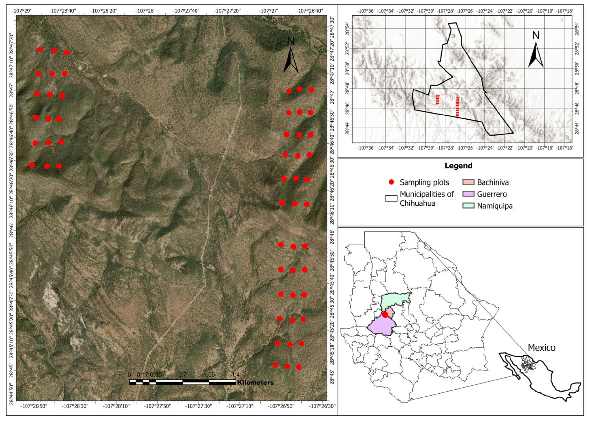
The study was conducted in the Teseachi Ranch, a research property of the Autonomous University of Chihuahua, located in the Sierra Madre Occidental of Chihuahua, Mexico (Figure 1). These forests are characterized mainly by oak and pine species, with a heterogeneous structure and varying levels of canopy density. The climate is classified as semi-dry temperate (BS1kw) according to the Köppen system modified by García, with a mean annual temperature of 14.8 °C and average annual precipitation of approximately 494 mm, of which nearly 80% occurs between June and October [23,24]. These conditions define a marked seasonality, with rainfall concentrated in the summer and extended dry periods during the rest of the year. Soils are classified as Haplic Phaeozems derived from igneous parent material, with loam-clay texture, moderate depth, and high infiltration capacity, which strongly influence hydrological processes [24]. The interaction between vegetation, soils, and climate results in a system where water availability is the primary limiting factor, with most rainfall lost through evapotranspiration and runoff occurring only during high-intensity events [24,25]. Additionally, the region presents relatively low atmospheric interference due to its elevation and climatic conditions, which is advantageous for remote sensing analyses.

Oak species, particularly Quercus arizonica Sarg, dominated the study area, whereas pine species exhibited lower abundance but larger average structural dimensions (

Table 1. Structural characteristics of tree species recorded in the study area.

Species	Abundance (Ind Plot−1)	DBH (cm)	HT (m)	CBH (m)	CD (m)
Quercus arizonica Sarg.	50.13 ± 32.49	20.00 ± 10.18	5.08 ± 1.55	1.28 ± 0.95	3.55 ± 1.50
Quercus sideroxyla Bonpl.	6.59 ± 13.78	18.68 ± 6.13	6.17 ± 1.57	1.73 ± 0.15	3.54 ± 1.33
Pinus arizonica Engelm.	2.85 ± 5.60	20.25 ± 6.93	6.67 ± 1.91	2.03 ± 0.99	3.77 ± 1.24
Pinus cembroides Zucc.	6.26 ± 8.11	21.25 ± 15.47	5.91 ± 2.52	1.29 ± 1.09	4.09 ± 1.63
Pinus engelmannii Carrière	0.26 ± 1.03	24.50 ± 8.64	8.01 ± 3.01	3.16 ± 1.75	4.76 ± 2.06
Pinus leiophylla Schiede ex Schltdl. & Cham.	1.43 ± 6.65	24.26 ± 7.95	8.62 ± 1.98	3.43 ± 1.10	4.35 ± 1.63
Juniperus deppeana Steud.	3.65 ± 5.31	15.44 ± 9.72	4.27 ± 1.42	0.79 ± 0.54	3.27 ± 1.13
Arbutus xalapensis Kunth	1.65 ± 2.88	21.00 ± 14.03	4.84 ± 1.50	1.41 ± 0.51	4.13 ± 2.53

Note: DBH = diameter at breast height; AT = total tree height; CBH = clear bole height; CD = crown diameter. Values are presented as mean ± standard deviation.

). This variability in species composition and canopy structure likely contributed to the heterogeneous spectral and biomass patterns observed throughout the study area.

The forests evaluated in this study have not been subjected to commercial timber harvesting for approximately 40 years, with extensive livestock grazing representing the primary land-use activity within the area. This condition is characteristic of many oak–pine transition forests in northern Mexico, where forest management activities are generally limited due to low timber productivity. These ecosystems commonly exhibit annual timber increments below 1 m³ ha⁻¹ year⁻¹, making commercial harvesting economically marginal and, in many cases, financially unfeasible.

2.2. Field Data Collection

Field data were collected using a clustered sampling design consisting of three spatially distributed clusters. The original sampling scheme included 18 sites per cluster (n = 54). However, logistical and site accessibility constraints prevented access to all planned locations. Consequently, 16 sites were sampled in two clusters and 17 sites in the third cluster, resulting in a final sample size of 49 sites. Within each cluster, sample sites were arranged along three North–South-oriented transects, with 150 m spacing between transects and 300 m spacing between adjacent sites. Site locations were selected to capture the environmental variability of the study area, including differences in vegetation density, elevation, and slope exposure. Field measurements were conducted between 1 October 2025, and 31 January 2026, corresponding to the period used for Sentinel-2 image acquisition and spectral index generation.

At each site, live woody vegetation was assessed within a circular plot of 1000 m² (17.84 m radius). All trees taller than 3 m were measured and recorded. The dendrometric variables collected included diameter at breast height (DBH, cm), total tree height (H, m), clear bole height (CBH, m), and crown diameter (CD, m). To characterize the shrub layer, three circular subplots of 38.4 m² (3.5 m radius) were established at azimuths separated by 120°. Within each subplot, shrub abundance was recorded, and measurements of total height, basal diameter and crown diameter were obtained.

The geographic coordinates of each sampling site were recorded using a Garmin GPSMAP 62s handheld receiver. Coordinates were acquired under acceptable satellite geometry conditions (PDOP ≤ 6) and subsequently used to spatially match field plots with Sentinel-2 imagery and extract the corresponding spectral information.

2.2.1. Volume and Aboveground Live Biomass Estimation

Aboveground biomass of tree species was estimated using species-specific allometric models obtained from the “Sistema Biométrico Forestal para México (SIBIFOR)”, which provides biometric models developed for Mexican forest ecosystems [19]. Appropriate models were selected according to the species composition of the study area. Tree volume was estimated from diameter at breast height (DBH) and total height using the corresponding allometric models and subsequently converted to aboveground biomass using a wood density factor representative of the dominant species present in the study area [26]. Shrub biomass was estimated independently using allometric models based on shrub structural attributes [27]. Biomass estimates were aggregated at the sampling-point level and converted to Mg ha⁻¹ according to the effective sampling area. Detailed model coefficients are provided in Supplementary Table S1.

2.2.2. Surface Fuel Biomass Estimation

Surface fuel loads were quantified by separating downed woody debris and the organic forest floor layer. Downed woody debris was estimated using the planar intersect method developed by Brown (1974) [4] and adapted for Mexican forest conditions by Sánchez and Zerecero [28]. Within each shrub subplot, three 15 m transects were established, resulting in a total of nine sampling transects per sampling point. Intersected woody material was classified into standard timelag fuel categories (1 h, 10 h, 100 h, and 1000 h fuels) according to particle diameter. Fuel loads were calculated from the frequency of intersections recorded along the transects following the corresponding planar-intersect equations.

Forest floor biomass was estimated through destructive sampling conducted at the end of each transect using 30 × 30 cm quadrats. Litter and fermentation layers were collected separately, transported to the laboratory, and oven-dried at 70 °C for 48 h or until constant weight was achieved. Dry weights were converted to biomass per unit area and expressed as Mg ha⁻¹. Total forest floor biomass was calculated as the sum of litter and fermentation layer biomass. Hereafter, this combined component is referred to as forest floor biomass throughout the manuscript.

2.2.3. Spectral Data Acquisition and Preprocessing

Sentinel-2 multispectral imagery was used to derive spectral information associated with aboveground live biomass and surface fuel components within the study area. The Sentinel-2 platform incorporates the Multispectral Instrument (MSI), which provides optical imagery at spatial resolutions of 10, 20, and 60 m, including visible, near-infrared (NIR), shortwave infrared (SWIR), and red-edge bands specifically designed for vegetation monitoring applications. The availability of red-edge bands makes Sentinel-2 particularly suitable for evaluating vegetation vigor, chlorophyll activity, canopy structure, and forest fuel characteristics in heterogeneous forest ecosystems.

Surface reflectance data were obtained from the Sentinel-2 Level-2A collection available within the Google Earth Engine (GEE) cloud-computing platform. The Level-2A product provides atmospherically corrected Bottom-of-Atmosphere (BOA) reflectance, enabling consistent quantitative spectral analyses across space and time. Imagery was spatially filtered to the study area and temporally constrained between 1 October 2025, and 31 January 2026. Only images with cloud cover lower than 20% were retained, and the Scene Classification Layer (SCL) algorithm was used to mask clouds, shadows, and low-quality observations. In addition to published vegetation indices, a weighted red–NIR normalized difference formulation (PVIα; α = 0.2) was implemented in Google Earth Engine to explore alternative vegetation-vigor responses under semi-arid forest conditions.

A total of 42 vegetation indices (VIs) were initially evaluated using Sentinel-2 imagery and subsequently grouped into four functional categories associated with chlorophyll activity, vegetation vigor, physiological condition, and soil/background correction effects (Supplementary Tables S2–S5). This classification was designed to represent complementary spectral responses related to biomass accumulation, vegetation condition, and surface fuel characteristics in heterogeneous forest ecosystems.

To reduce missing observations and improve spatial consistency, cloud-free image composites were generated within the selected temporal window. Spectral information was extracted by assigning each field sampling plot to the Sentinel-2 pixel containing the plot center, as determined from georeferenced GPS coordinates. Reflectance values and vegetation indices associated with this central pixel were subsequently used in all statistical analyses.

2.2.4. Spectral Index Classification and Ecological Rationale

To improve ecological interpretability and reduce redundancy among highly correlated predictors, the evaluated vegetation indices were classified into four functional groups according to their primary spectral sensitivity and ecological response: chlorophyll-related indices, vegetation vigor indices, physiological indices, and soil/background correction indices (

Table 2. Functional classification of spectral indices used in biomass modeling.

Functional Group	Ecological Sensitivity	Included Spectral Indices	Main Application
Chlorophyll indices	Chlorophyll concentration, pigment activity, and red-edge response	MTCI, MTCI2, NDRE1, NDRE2, RENDVI, CIre7, CIre8A, REP1, VOG1, CCCI	Estimation of canopy productivity and photosynthetic activity
Soil/background correction indices	Reduction in soil reflectance and atmospheric effects	ARVI, EVI, EVI2, EVI5, OSAVI, RDVI	Improved spectral stability in heterogeneous forest conditions
Physiological indices	Plant stress, pigment degradation, and senescence processes	SIPI, MCARI, MTVI1, MTVI2, NPCI, TCARI, TGI	Detection of physiological condition and dry fuel accumulation
Vegetation vigor indices	Vegetation greenness, canopy density, and biomass accumulation	NDVI, NDVI1, NDVI2, NDVI3, NDVI4, NDVI5, NDVI6, SR, SR1, SR3, SR4, GNDVI, GNDVI2, GCI, CIgreen, CIg7, DVI, GLI, GIPVI, NVI1, PVIα	Estimation of vegetation vigor, canopy greenness, and red–NIR spectral gradients related to vegetation structure.

Note: Detailed descriptions, equations, and bibliographic references for all evaluated Sentinel-2 spectral indices are provided in Supplementary Table S5.

). This classification framework was established based on previous studies describing the spectral behavior, ecological interpretation, and intended applications of vegetation indices in biomass estimation, vegetation monitoring, and canopy characterization. Accordingly, indices were grouped according to their dominant spectral sensitivity rather than their mathematical formulation [12,13,15,16,17]. Chlorophyll-related indices were associated with chlorophyll concentration and red-edge reflectance dynamics, whereas vegetation vigor indices primarily represented vegetation greenness, canopy density, and biomass accumulation. Physiological indices were related to vegetation stress, pigment degradation, and senescence processes, while soil/background correction indices were designed to minimize soil reflectance, atmospheric interference, and spectral saturation effects under heterogeneous vegetation conditions.

2.2.5. Spectral Predictor Selection and Modeling Framework

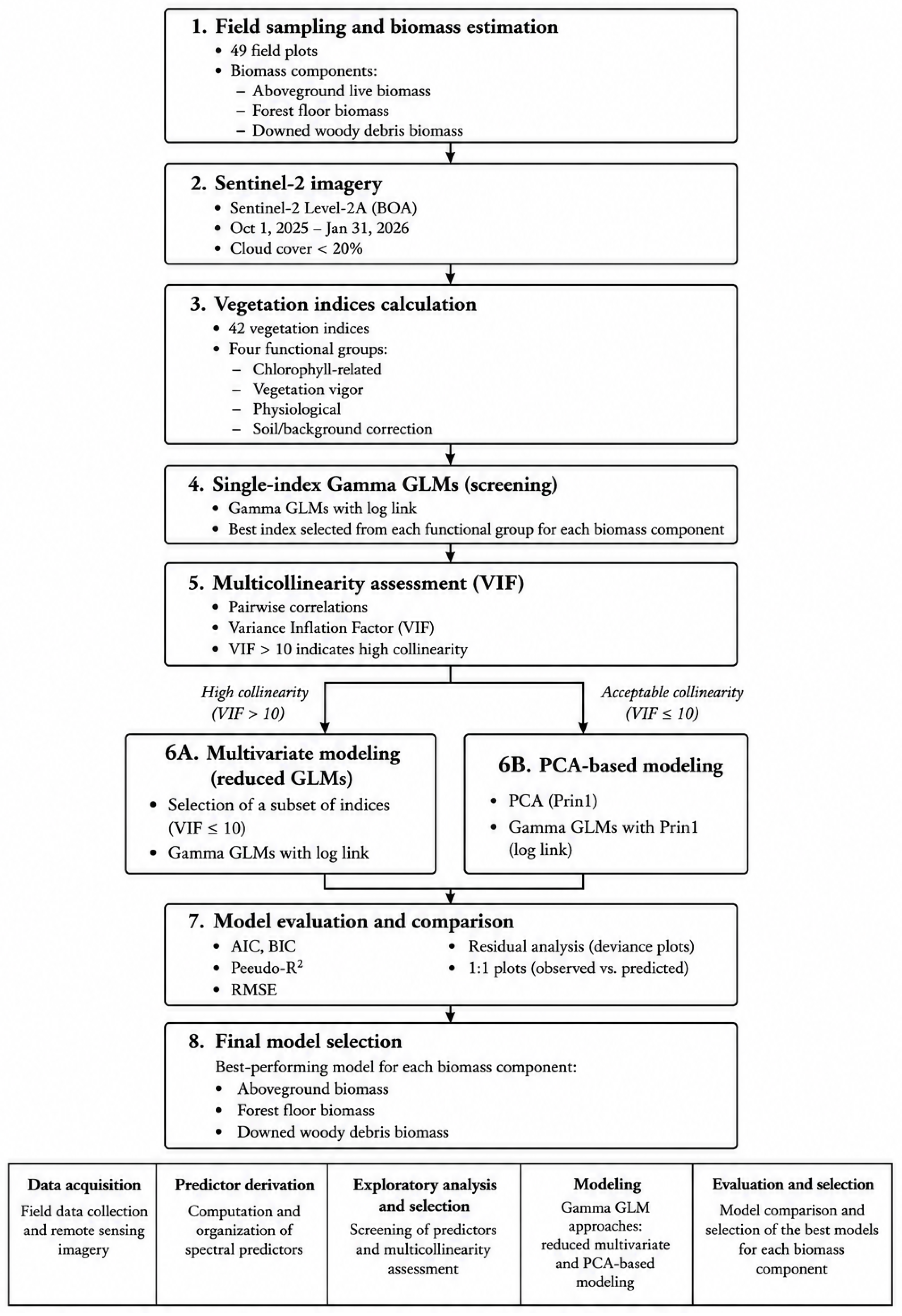
The overall analytical workflow adopted in this study is summarized in Figure 2. The workflow illustrates the sequential analytical procedure followed to identify the most informative spectral predictors for each biomass component, including vegetation index classification, single-index Gamma GLM screening, multicollinearity assessment, reduced multivariate and PCA-based modeling, model evaluation, and final model selection. This schematic overview is intended to facilitate understanding of the methodological sequence described below.

Relationships between spectral predictors and biomass components (aboveground live biomass, forest floor biomass, and downed woody debris) were evaluated using Generalized Linear Models (GLMs) with Gamma distribution and logarithmic link function, which were selected due to the continuous, positive, and right-skewed nature of biomass data.

Initially, all evaluated Sentinel-2 spectral indices were independently tested for each biomass component using single-index Gamma GLMs. Model performance was compared using Akaike Information Criterion (AIC), corrected Akaike Information Criterion (AICc), Bayesian Information Criterion (BIC), Deviance/DF, Pearson χ²/DF, and parameter significance. Spectral indices were not selected as a single overall best predictor. Instead, for each biomass component, the best-performing index within each functional spectral group was retained. This procedure resulted in four selected indices per biomass component, representing chlorophyll-related, soil/background correction, vegetation vigor, and physiological responses. This group-based selection strategy was used to preserve complementary ecological information while reducing redundancy among highly correlated spectral predictors.

After this initial screening, reduced multivariate Gamma GLMs were fitted using combinations of selected indices that provided complementary ecological information and acceptable parameter stability. Models including the four selected indices simultaneously showed high inter-index correlations and elevated Variance Inflation Factor (VIF) values, indicating substantial multicollinearity and unstable parameter estimates. Therefore, reduced two-index multivariate models were retained for comparative purposes. In parallel, Principal Component Analysis (PCA) was applied to the four selected indices for each biomass component to integrate their shared spectral information into orthogonal variables. The first principal component (Prin1), which explained most of the total spectral variance, was subsequently used as an integrated predictor in PCA-based Gamma GLMs. PCA was applied to the best-performing representative indices from each ecological group in order to preserve ecological interpretability while reducing multicollinearity.

Model performance and predictive capacity were evaluated using AIC, BIC, Pearson χ² statistics, Deviance statistics, Root Mean Square Error (RMSE), McFadden’s R², residual diagnostics, and observed-versus-predicted relationships.

Residual diagnostics included residual mean deviation, skewness and kurtosis statistics, residual-versus-fitted analyses, and three complementary normality tests (Kolmogorov–Smirnov, Cramer–von Mises, and Anderson–Darling) to evaluate the distributional properties of model residuals and verify the adequacy of the fitted Gamma GLMs.

Influential observations were identified using Cook’s distance, applying the commonly used threshold of 4/n, where n is the number of observations. Observations exceeding this threshold were considered potentially influential and were temporarily excluded to evaluate their effect on parameter estimates, model fit, and predictive performance. Candidate models were fitted using both the complete dataset and the reduced dataset excluding influential observations. Final model selection was based on statistical parsimony, residual diagnostics, predictor significance, predictive performance, and ecological interpretability.

2.2.6. Statistical Equations and Model Formulation

The general formulation of the Gamma GLMs used for biomass estimation is presented below. Expected biomass means were obtained by exponentiating the linear predictor under the logarithmic link function:

μ_i = exp(η_i)

(1)

where μ_i represents expected biomass mean and η_i the linear predictor (β₀ + β₁ X₁ + ⋯ + β_n X_n).

The statistical formulations corresponding to the single-index, multivariate, and PCA-based Gamma GLMs used in this study are summarized in

Table 3. Statistical models, analytical expressions, and evaluation metrics used in this study.

Category	Method/Metric	Analytical Expression
Statistical Model	Gamma GLM	log(μi) = β0 + β1Xi
	Multivariate Gamma GLM	log(μi) = β0 + β1X1 + β2X2 + ⋯ + βnXn
	PCA-based Gamma GLM	log(μi) = β0 + β1Prin1
Dimension reduction	Principal Component	Prin1 = a1X1 + a2X2 + ⋯ + anXn
Evaluation metric	Root Mean Square Error	RMSE = √[(1/n)Σ(yi − ŷi)2]
Diagnostic metric	Variance Inflation Factor	VIF = 1/(1 − R2)

Abbreviations: GLM, Generalized Linear Model; PCA, Principal Component Analysis; Prin1, first principal component; RMSE, Root Mean Square Error; VIF, Variance Inflation Factor. β₀ denotes the intercept, β₁–β_n denote regression coefficients, X₁–X_n denote predictor variables, a₁–a_n denote principal component loadings, μ_i denotes the expected response for observation i, y_i and ŷ_i denote observed and predicted values, respectively, n is the sample size, and R² is the coefficient of determination.

.

The three complementary GLM strategies evaluated for each biomass component are summarized in

Table 4. Summary of GLM modeling strategies evaluated for each biomass component.

Biomass Component	Model Type	Predictors Included	Objective
Aboveground live biomass	Single-index GLM	CIre8A	Evaluate the best individual spectral predictor
	Multivariate GLM	CIre8A + NDVI4	Evaluate a reduced multivariate model after excluding highly collinear predictors
	PCA-based GLM	Prin1 derived from CIre8A, EVI2, NDVI4, and SIPI	Integrate the four selected functional spectral groups while reducing multicollinearity
Forest floor biomass	Single-index GLM	NPCI	Evaluate the best individual spectral predictor
	Multivariate GLM	NDVI + NPCI	Evaluate a reduced multivariate model after excluding highly collinear predictors
	PCA-based GLM	Prin1 derived from RENDVI, ARVI, NDVI, and NPCI	Integrate the four selected functional spectral groups while reducing multicollinearity
Downed woody debris	Single-index GLM	ARVI	Evaluate the best individual spectral predictor
	Multivariate GLM	PVIα + NPCI	Evaluate a reduced multivariate model after excluding highly collinear predictors
	PCA-based GLM	Prin1 derived from RENDVI, ARVI, PVIα, and NPCI	Integrate the four selected functional spectral groups while reducing multicollinearity

. For each biomass component, the best-performing individual spectral index was first evaluated using single-index Gamma GLMs. Subsequently, reduced multivariate models were fitted using two selected indices that provided complementary ecological information while minimizing instability caused by high collinearity among the four functional spectral groups. Finally, PCA-based GLMs were fitted using the first principal component (Prin1), derived from the four selected indices representing chlorophyll, soil/background correction, vegetation vigor, and physiological responses.

3. Results

3.1. Spectral Index Evaluation and Selection

Distinct spectral responses were observed among biomass components, indicating that the predictive performance of Sentinel-2 indices depended on the ecological and structural characteristics of each fuel type. For each biomass category, one representative index from each functional spectral group was selected according to model fit statistics and parameter significance criteria (

Table 5. Selected spectral indices and model fit statistics for each biomass component.

Biomass Component	Functional Group	Selected Index	AIC	BIC	Deviance/DF	Pearson χ2/DF	p-Value
Aboveground live biomass	Chlorophyll	CIre8A	459.6534	465.3289	0.3359	0.3543	0.0019
	Soil/background correction	EVI2	456.4565	462.1319	0.3156	0.3343	0.0003
	Vegetation vigor	NDVI4	461.1528	466.8283	0.3458	0.3736	0.0042
	Physiological	SIPI	459.5476	465.223	0.3352	0.3644	0.0019
Forest floor biomass	Chlorophyll	RENDVI	222.7216	228.3971	0.3897	0.3481	0.01
	Soil/background correction	ARVI	219.2465	224.9219	0.3644	0.3202	0.0012
	Vegetation vigor	NDVI	223.239	228.9145	0.3936	0.3651	0.0131
	Physiological	NPCI	217.5109	223.1864	0.3523	0.3327	0.0003
Downed woody debris	Chlorophyll	RENDVI	289.8162	295.4917	0.3386	0.369	<0.0001
	Soil/background correction	ARVI	283.0512	288.7266	0.2968	0.3525	<0.0001
	Vegetation vigor	PVIα	288.2084	293.8839	0.3282	0.3679	<0.0001
	Physiological	NPCI	286.6104	292.2859	0.3181	0.3707	<0.0001

Note: AIC = Akaike Information Criterion; BIC = Bayesian Information Criterion; Deviance/DF = deviance divided by degrees of freedom; Pearson χ²/DF = Pearson chi-square divided by degrees of freedom.

). Complete rankings and statistical performance metrics for all evaluated spectral indices are provided in Supplementary Tables S2–S4.

Aboveground live biomass was primarily associated with indices related to chlorophyll activity and vegetation vigor, whereas forest floor biomass and downed woody debris showed stronger relationships with physiological and soil/background correction indices. In particular, NPCI and PVIα emerged as the most informative predictors for dead fuel components, while CIre8A, EVI2, and NDVI4 showed stronger associations with aboveground live biomass.

Overall, the selected indices provided the basis for subsequent Gamma GLM and PCA-based modeling analyses.

Influential observations were identified using Cook’s distance, applying the commonly used threshold of 4/n (0.0816 for n = 49). Five observations (10.2% of the dataset; site IDs 15, 16, 17, 26, and 40) exceeded this threshold and were considered potentially influential. Cook’s distance values for these observations ranged from 0.084 to 0.203 depending on the model. To evaluate the robustness of model selection, all candidate models were fitted using both the complete dataset (n = 49) and a reduced dataset excluding influential observations (n = 44). Removal of influential observations improved model fit and predictive performance, as reflected by lower AIC values and reduced prediction errors, while preserving the relative ranking of competing models. Final model selection was based on statistical parsimony, residual diagnostics, predictor significance, predictive performance, and ecological interpretability.

3.2. Model Evaluation and Selection

The Gamma generalized linear models (GLMs) fitted for aboveground live biomass, forest floor biomass, and downed woody debris revealed substantial differences in the predictive performance and statistical robustness of the evaluated spectral indices (

Table 6. GLM Gamma parameter estimates and statistical significance.

Biomass Component	Model	Parameter	Estimate	Standard Error	Wald χ2	p-Value
Aboveground live biomass	CIre8A	Intercept	1.9608	0.454	18.65	<0.0001
		CIre8A	6.3227	1.5633	16.36	<0.0001
	CIre8A + NDVI4	Intercept	2.0845	0.5549	14.11	0.0002
		CIre8A	5.0301	3.6517	1.9	0.1684
		NDVI4	2.2316	5.689	0.15	0.6949
	PCA-Prin1	Intercept	3.7722	0.0699	2912.84	<0.0001
		Prin1	0.1594	0.0385	17.14	<0.0001
Forest floor biomass	NDVI	Intercept	−0.0832	0.4357	0.04	0.8486
		NDVI	5.9939	1.7533	11.69	0.0006
	NDVI + NPCI	Intercept	1.726	1.0654	2.62	0.1052
		NDVI	1.6465	2.8623	0.33	0.5651
		NPCI	−6.4879	3.5345	3.37	0.0664
	PCA-Prin1	Intercept	1.4305	0.0867	272.03	<0.0001
		Prin1	0.1806	0.0546	10.93	0.0009
Downed woody debris	PVIα	Intercept	−14.8861	2.8858	26.61	<0.0001
		PVIα	21.8846	3.7163	34.68	<0.0001
	PVIα + NPCI	Intercept	−4.137	4.6923	0.78	0.378
		PVIα	9.0493	5.7352	2.49	0.1146
		NPCI	−7.3725	2.6824	7.55	0.006
	PCA-Prin1	Intercept	2.0854	0.0662	992.95	<0.0001
		Prin1	0.276	0.0401	47.37	<0.0001

). For aboveground live biomass, both the CIre8A index and the PCA-derived predictor (Prin1) exhibited highly significant effects (p < 0.0001), indicating a strong association between spectral responses related to chlorophyll concentration, canopy physiological vigor, and live biomass accumulation. The positive parameter estimates obtained for CIre8A and Prin1 further indicate that increases in vegetation vigor and photosynthetically active biomass were directly associated with higher aboveground live biomass values. Conversely, models incorporating multiple spectral predictors displayed reduced individual parameter significance. In particular, the CIre8A + NDVI4 model yielded non-significant coefficients for both variables despite the recognized ecological relevance of these indices. This pattern strongly suggests the presence of multicollinearity and redundancy among highly correlated spectral predictors, thereby diminishing the independent explanatory contribution of each variable within the model structure.

For forest floor biomass and downed woody debris, PCA-derived models consistently exhibited the highest statistical stability and explanatory coherence across biomass categories. In all cases, the first principal component (Prin1) remained highly significant (p < 0.001), with especially pronounced effects observed for downed woody debris (Wald χ² = 47.37). These results indicate that principal component analysis effectively synthesized complex spectral variability associated with vegetation senescence, structural fuel heterogeneity, and surface condition gradients.

Individual spectral indices likewise exhibited differentiated ecological responses according to biomass component. NDVI showed a significant positive relationship with forest floor biomass, reflecting its sensitivity to residual vegetation cover and surface organic material. In contrast, NPCI displayed negative parameter estimates in dead fuel models, suggesting sensitivity to pigment degradation processes and the accumulation of dry organic matter. Similarly, PVIα demonstrated strong positive associations with downed woody debris, likely reflecting enhanced sensitivity to exposed dry vegetation, structural fuel elements, and soil background effects characteristic of sparsely vegetated environments.

Collectively, PCA-derived predictors provided the most consistent and statistically robust performance across biomass categories, underscoring the utility of dimensionality reduction approaches for modeling heterogeneous fuel components in arid and semi-arid ecosystems characterized by high spectral and structural complexity.

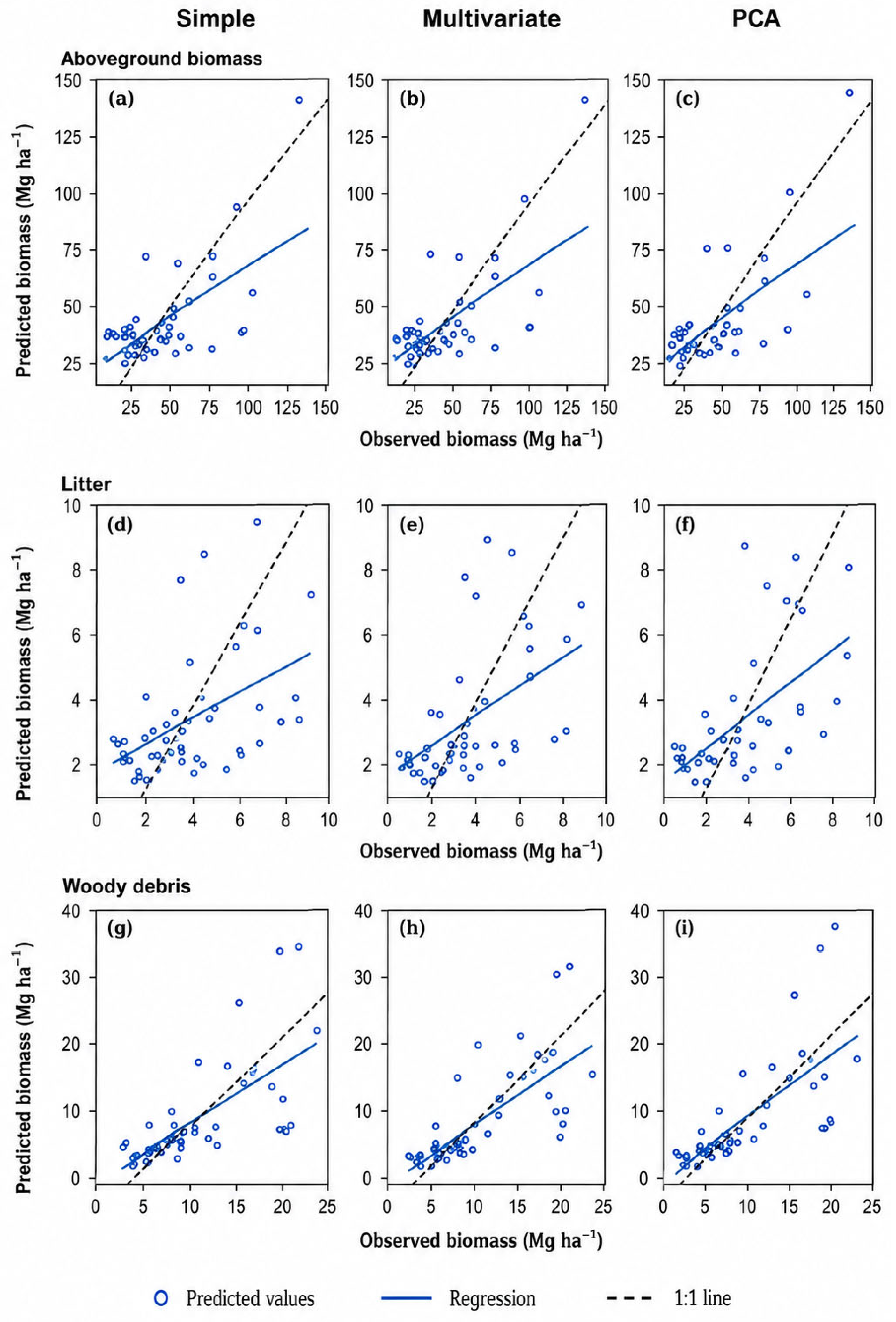
Beyond parameter significance, model predictive performance was further evaluated through observed-versus-predicted relationships in order to assess the consistency, dispersion, and overall predictive behavior of the evaluated GLMs across biomass components.

Observed-versus-predicted relationships showed that PCA-based GLMs generally produced more stable and consistent predictive behavior across biomass components, particularly for forest floor biomass and downed woody debris. Aboveground live biomass models exhibited greater dispersion at higher biomass values, whereas forest floor biomass models showed moderate predictive capacity with increased variability among observations. In contrast, downed woody debris models displayed the strongest agreement between observed and predicted values, especially under PCA-based formulations, indicating improved representation of dead fuel variability through integrated spectral information. Overall, PCA-based models reduced residual dispersion and improved prediction consistency relative to single-index and multivariate approaches (Figure 3).

3.3. Model Fit and Validation

Goodness-of-fit statistics indicated that PCA-based models consistently produced the lowest AIC and BIC values across the evaluated biomass components, indicating improved model parsimony and overall fit (

Table 7. GLM Gamma model fit and validation statistics.

Biomass Component	Model	AIC	BIC	RMSE	Pearson χ2	Pearson χ2/DF	Deviance/DF	McFadden Pseudo-R2	VIF
Aboveground live biomass	CIre8A	389.547	394.8995	19.4394	9.1501	0.2179	0.2385	0.0409	1
	CIre8A + NDVI4	391.3922	398.529	19.4841	9.2659	0.226	0.2435	0.0413	>10
	PCA-Prin1	388.5218	393.8744	19.6196	9.247	0.2202	0.2332	0.0435	1
Forest floor biomass	NDVI	195.375	200.7949	4.4144	12.2471	0.2848	0.3443	0.041	1
	NDVI + NPCI	194.0068	201.2335	4.3828	11.8034	0.281	0.3282	0.047	4.16
	PCA-Prin1	193.8421	199.262	4.3763	11.5217	0.2679	0.3214	0.051	1
Downed woody debris	PVIα	261.6885	267.2389	5.0775	11.7292	0.2606	0.2586	0.073	1
	PVIα + NPCI	256.3916	263.7922	5.0385	9.654	0.2194	0.2277	0.0918	3.58
	PCA-Prin1	254.3319	259.8823	5.0392	9.5497	0.2122	0.2223	0.092	1

Note: AIC = Akaike Information Criterion; BIC = Bayesian Information Criterion; RMSE = root mean square error; Pearson χ²/DF = Pearson chi-square divided by degrees of freedom; Deviance/DF = deviance divided by degrees of freedom; McFadden pseudo-R² = likelihood-based pseudo coefficient of determination; VIF = variance inflation factor.

). Pearson χ²/DF and Deviance/DF values remained below 1 for all models, supporting the adequacy of the Gamma GLM framework and indicating the absence of overdispersion. Root mean square error (RMSE) values were relatively similar among competing models within each biomass category, suggesting comparable predictive precision among formulations. Nevertheless, PCA-based models generally exhibited lower residual dispersion while maintaining reduced model complexity and stable parameter estimates. Likewise, McFadden pseudo-R² values, although modest in magnitude, were consistently highest in PCA-based models, particularly for downed woody debris, reflecting improved relative explanatory performance under ecologically heterogeneous conditions. It is important to note that pseudo-R² statistics derived from likelihood-based GLMs are typically lower than conventional ordinary least squares (OLS) R² values and should be interpreted primarily as comparative indicators of relative model improvement rather than direct measures of explained variance [29,30].

Multivariate models combining multiple spectral predictors exhibited increased VIF values, particularly for aboveground live biomass, where the CIre8A + NDVI4 model showed severe multicollinearity (VIF > 10). In contrast, PCA-based models eliminated collinearity effects (VIF = 1) while maintaining significant parameter estimates and stable predictive performance. Collectively, these results indicate that PCA-based formulations provided the most statistically robust, parsimonious, and internally consistent modeling framework across biomass components.

Residual analyses indicated that all fitted models produced residuals centered near zero, with non-significant t-tests (p > 0.05), suggesting the absence of systematic prediction bias (

Table 8. Residual diagnostics and normality assessment.

Biomass Component	Model	Residual Mean	Residual SD	Skewness	Kurtosis	p-Value t	p-Value KS	p-Value CvM	p-Value AD
Aboveground live biomass	CIre8A	−0.074	0.477	−0.150	−0.174	0.312	>0.150	>0.250	>0.250
	CIre8A + NDVI4	−0.073	0.476	−0.102	−0.136	0.312	>0.150	>0.250	>0.250
	PCA-Prin1	−0.072	0.472	−0.048	−0.130	0.315	>0.150	>0.250	>0.250
Forest floor biomass	NDVI	−0.082	0.521	0.015	−0.215	0.267	>0.150	>0.250	>0.250
	NDVI + NPCI	−0.080	0.504	0.068	−0.338	0.278	>0.150	>0.250	>0.250
	PCA-Prin1	−0.076	0.498	−0.052	−0.287	0.294	>0.150	>0.250	>0.250
Downed woody debris	PVIα	−0.081	0.496	0.131	0.427	0.271	>0.150	>0.250	>0.250
	PVIα + NPCI	−0.069	0.461	−0.026	0.263	0.309	0.1073	>0.250	>0.250
	PCA-Prin1	−0.069	0.461	−0.049	0.187	0.310	>0.150	>0.250	>0.250

Note: Residual SD = standard deviation of residuals; KS = Kolmogorov–Smirnov test; CvM = Cramer–von Mises test; AD = Anderson–Darling test. Skewness and Kurtosis describe the symmetry and tail behavior of residual distributions, respectively.

). Skewness and kurtosis values remained close to zero across models, indicating approximately symmetric residual distributions without severe tail behavior. Normality tests, including Kolmogorov–Smirnov, Cramer–von Mises, and Anderson–Darling statistics, detected no substantial departures from normality. Among the evaluated approaches, PCA-based models consistently exhibited lower residual dispersion and more stable residual behavior across biomass components, supporting their overall statistical robustness.

3.4. PCA Analysis

Principal component analysis identified a dominant first principal component (Prin1) for each biomass component.

Table 9. Principal component analysis and spectral contribution of Prin1.

Biomass Component	Spectral Index	Mean	Std. Dev.	Loading Prin1
Aboveground live biomass	CIre8A	0.29049	0.04956	0.50479
	NDVI4	0.11323	0.03304	0.49273
	EVI2	0.11176	0.01896	0.49634
	SIPI	0.46461	0.03397	0.50602
Forest floor biomass	RENDVI	0.1433	0.02271	0.49006
	ARVI	0.06731	0.05483	0.51666
	NDVI	0.24394	0.05098	0.51101
	NPCI	0.11714	0.04195	−0.48143
Downed woody debris	RENDVI	0.15098	0.03233	0.49731
	ARVI	0.08285	0.07032	0.51411
	NPCI	0.10883	0.04627	−0.47893
	PVIα	0.7763	0.02224	0.50892

presents the loading coefficients, means, and standard deviations used to calculate Prin1, allowing reproducible computation of the PCA-derived predictor. Loading patterns showed consistent differences between live and dead biomass components. For aboveground live biomass, all indices contributed positively to Prin1, whereas forest floor biomass and downed woody debris exhibited negative loadings for NPCI while vegetation vigor indices remained positively associated with the first component. Overall, Prin1 represented an integrated spectral gradient associated with vegetation condition and surface fuel characteristics.

Loading coefficients indicate the relative contribution and direction of association of each spectral index within the principal component structure, whereas mean and standard deviation values were used to standardize the original variables prior to PCA computation. For operational implementation of the PCA-based models, new observations must be standardized using the corresponding mean and standard deviation values reported in Table 9 and subsequently multiplied by their associated loading coefficients to obtain the Prin1 score also included in Table 9:

Z_i = (X_i − μ_i)/σ_i

(2)

Prin1 = Σ(Z_i L_i)

(3)

where X_i is the observed spectral index value, μ_i and σ_i correspond to the mean and standard deviation values reported in

Table 10. Eigenvalues and explained variance of principal components for biomass spectral models.

Biomass Component	Prin1 Eigenvalue	Proportion of Variance	Cumulative Variance
Aboveground live biomass	3.81	0.9525 (95.25%)	95.25%
Forest floor biomass	3.6118	0.9030 (90.30%)	90.30%
Downed woody debris	3.6923	0.9231 (92.31%)	92.31%

, and L_i represents the associated Prin1 loading coefficient. This procedure enables reproducible calculation of PCA-derived predictors for subsequent biomass estimation using the fitted Gamma GLMs.

As shown in Table 10, the first principal component (Prin1) explained between 90.30% and 95.25% of the total spectral variance across the three biomass components, indicating strong redundancy among the evaluated spectral indices. These results support the use of PCA as an effective dimensionality reduction approach by concentrating most spectral variability into a single orthogonal predictor.

The high eigenvalues associated with Prin1 further confirmed its capacity to summarize the shared spectral information contained in the original predictors. Consequently, the use of Prin1 as a synthetic predictor improved model parsimony and reduced multicollinearity in the Gamma GLM analyses.

4. Discussion

The present study suggest that different biomass components exhibit distinct spectral responses according to their ecological and structural characteristics, supporting our initial hypothesis and highlighting the complexity of remotely estimating surface fuels and aboveground live biomass in heterogeneous dry oak–pine forests. Aboveground live biomass was primarily associated with indices linked to vegetation vigor, chlorophyll concentration, and canopy structure, whereas forest floor biomass and downed woody debris exhibited stronger relationships with indices sensitive to senescence, dry organic matter, soil exposure, and background correction effects. These results indicate that the spectral behavior of forest fuels is strongly dependent on the ecological condition and physical arrangement of biomass components within the forest structure, which is consistent with previous studies reporting contrasting optical properties between live vegetation and senescent or dead organic material [31,32,33].

For aboveground live biomass, the strong performance of CIre8A and NDVI4 suggests that red-edge reflectance and canopy vigor are dominant drivers of spectral variability in dry oak–pine forests. Red-edge indices are highly sensitive to chlorophyll concentration and photosynthetic activity and are particularly effective under heterogeneous canopy conditions where traditional greenness indices may experience saturation effects under moderate-to-high biomass conditions [6,9,34]. In semi-arid forests such as those evaluated in this study, canopy cover is frequently discontinuous and structurally irregular due to water limitation, variable tree density, and species-specific physiological responses characteristic of semi-arid forests [35,36]. Consequently, subtle differences in canopy vigor and crown structure become highly relevant for explaining spectral variability associated with aboveground live biomass accumulation. The significant contribution of chlorophyll-related indices therefore reflects the strong relationship between photosynthetically active vegetation and total live biomass in these ecosystems.

In contrast, forest floor biomass and downed woody debris showed distinct spectral patterns associated with dry organic matter accumulation, senescence processes, and heterogeneous surface conditions, as previously documented for senescent vegetation and decomposing surface fuels [33,37]. Indices such as NPCI and PVIα exhibited greater importance for dead fuel estimation, suggesting that spectral responses associated with pigment degradation, vegetation condition, and dry surface material play a fundamental role in representing surface fuels. The relevance of NPCI is ecologically meaningful because this index is sensitive to the carotenoid-to-chlorophyll ratio and therefore reflects vegetation stress and senescent organic material [16]. Likewise, the importance of ARVI, originally developed to reduce atmospheric effects and improve vegetation signal retrieval under heterogeneous background conditions [38,39], indicates that background correction becomes critical in dry forests characterized by discontinuous vegetation cover, exposed substrate, shadows, and heterogeneous distributions of downed woody debris. The favorable performance of PVIα for downed woody debris estimation suggests that weighted red–NIR formulations may capture spectral variability associated with exposed woody material, litter accumulation, and heterogeneous surface conditions. Although PVIα was classified within the vegetation-vigor group because of its normalized red–NIR formulation, its strongest relationships were observed for downed woody debris. This result suggests that red–NIR spectral gradients may also respond to the combined effects of woody debris accumulation, partial canopy cover, and vegetation senescence in semi-arid oak–pine forests. Although PVIα differs from the original Perpendicular Vegetation Index formulation [40], its weighting structure appears to enhance sensitivity to dead surface fuel conditions under these heterogeneous environmental conditions.

These findings suggest that dead fuels cannot be adequately represented solely through conventional vegetation vigor indices because their spectral behavior is influenced by multiple interacting factors, including decomposition state, soil exposure, moisture variability, and partial canopy cover.

PCA-based models consistently provided the most parsimonious and statistically stable modeling framework, reducing multicollinearity while maintaining predictive performance comparable to or better than single-index and multivariate formulations. Although individual spectral indices provided statistically significant relationships with biomass components, multivariate models frequently exhibited reduced parameter significance and elevated VIF values due to strong spectral redundancy among vegetation indices derived from similar Sentinel-2 bands. In contrast, PCA-based models eliminated multicollinearity problems while maintaining model stability, significant parameters, and improved goodness-of-fit statistics. Ecologically, this result suggests that forest biomass and surface fuels are not represented by isolated spectral responses, but rather by integrated ecological gradients involving vegetation vigor, canopy structure, physiological condition, senescence, and soil exposure. In structurally heterogeneous semi-arid forests, live vegetation, dry fuels, shadows, and exposed soil commonly coexist within the same Sentinel-2 pixel, generating complex spectral mixtures typical of heterogeneous dry forests [41,42]. Under these conditions, dimensionality reduction approaches such as PCA may better capture integrated ecological gradients controlling spectral variability.

The high proportion of variance explained by the first principal component further supports the existence of a dominant latent spectral gradient associated with biomass and fuel dynamics. Positive loadings for indices related to vegetation vigor and chlorophyll activity, combined with negative loadings for senescence-related indices such as NPCI, indicate that PCA effectively represented the ecological transition between active vegetation and dry or degraded organic material. This spectral gradient likely reflects underlying processes of productivity, forest floor biomass accumulation, vegetation stress, and fuel desiccation, supporting previous findings indicating that the integration of vigor and senescence-related indices improves biomass and fuel estimation in heterogeneous ecosystems [7]. In semi-arid ecosystems, where green vegetation and dry fuels coexist spatially during extended dry periods, integrating both spectral responses becomes particularly important for representing ecosystem condition and fuel dynamics.

From an ecological and management perspective, the results obtained in this study are particularly relevant for dry oak–pine forests of northern Mexico. These ecosystems commonly occur at lower elevations within the Sierra Madre Occidental, where temperatures are generally higher and annual precipitation lower than in higher elevation pine-dominated forests, as documented for climatic and hydrological gradients in the Sierra Madre Occidental of Chihuahua [24,25,43]. Such climatic conditions favor prolonged dry periods, fuel desiccation, and elevated wildfire risk under ongoing climate warming and increasing drought severity [24,44]. Additionally, many of these forests exhibit limited commercial timber harvesting because of their relatively low timber productivity and slow growth rates. As a consequence, large quantities of forest floor biomass and woody surface fuels may accumulate over long periods in the absence of intensive forest management activities. Under current climate warming scenarios, these conditions may substantially increase wildfire frequency, fire intensity, and ecosystem vulnerability in semi-arid forests of northern Mexico.

Beyond their application to wildfire risk assessment, the biomass components evaluated in this study represent ecologically distinct carbon pools that differ in carbon residence time, decomposition dynamics, and ecosystem function. Accurate estimation of aboveground live biomass, forest floor biomass, and downed woody debris may therefore contribute to improving carbon accounting, monitoring ecosystem carbon stocks, and supporting climate change mitigation strategies in semi-arid forest ecosystems. Because these biomass fractions respond differently to disturbance and decomposition processes, their separate assessment may provide more informative estimates of forest carbon dynamics than approaches based solely on total aboveground biomass.

The capacity to estimate aboveground live biomass, forest floor biomass, and downed woody debris using freely available Sentinel-2 imagery therefore represents an important contribution for ecological monitoring and fuel management in fire-prone ecosystems. Traditional fuel inventories based on destructive sampling, laboratory procedures, and planar intersect methods require substantial field effort, specialized personnel, and considerable economic investment, particularly when destructive sampling and planar intersect methods are implemented in structurally heterogeneous forests [4,5]. In the present study, field data collection involved detailed forest inventories, destructive forest floor biomass sampling followed by laboratory drying procedures, and planar intersect fuel measurements for downed woody debris quantification. These methodologies are highly labor-intensive and time-consuming, especially in structurally heterogeneous dry forests where fuel distribution is spatially irregular. Consequently, despite the moderate sample size, the dataset represents a substantial field and laboratory effort with high ecological detail and measurement precision.

Although the number of sampling plots was relatively limited, model diagnostics indicated stable residual behavior, low dispersion, and statistically consistent parameter estimates. Nevertheless, some limitations should be acknowledged. The moderate sample size may restrict the generalization capacity of the models under broader environmental conditions, and the spatial resolution of Sentinel-2 may not fully capture fine-scale heterogeneity associated with surface fuel distribution beneath discontinuous canopies. Additionally, fuel moisture conditions and seasonal phenological variability may influence spectral responses over time, potentially affecting model transferability across seasons or years. Future studies should therefore incorporate larger datasets, multi-seasonal imagery, independent validation procedures, and complementary remote sensing technologies such as LiDAR or hyperspectral data to further improve fuel estimation accuracy and spatial representation.

Although additional validation under broader environmental conditions would further strengthen the applicability of these models, particularly since an independent dataset for external validation was not available in the present study, the results provide a useful methodological and empirical basis for biomass and surface fuel estimation in ecosystems with characteristics similar to those evaluated here. Future research may benefit from incorporating independent datasets, multi-seasonal imagery, and complementary remote sensing technologies such as LiDAR or hyperspectral data to further evaluate model transferability across different environmental conditions.

Overall, our results demonstrate that the spectral response of forest biomass and surface fuels is strongly dependent on ecological fuel characteristics and that integrated spectral approaches based on PCA and Gamma GLMs provide robust alternatives for biomass estimation in heterogeneous semi-arid forests. The integration of chlorophyll-related, vegetation vigor, physiological, and soil/background correction indices allowed the identification of distinct spectral mechanisms associated with live and dead biomass components. These findings contribute to improving ecological interpretation of remote sensing signals in dry forests and provide valuable information for wildfire risk assessment, fuel management, carbon monitoring, and ecosystem conservation in oak–pine forests increasingly exposed to drought and climate warming.

5. Conclusions

Distinct biomass components exhibited contrasting spectral responses. Aboveground live biomass was primarily associated with chlorophyll-related spectral responses, whereas forest floor biomass and downed woody debris were more closely related to indices associated with vegetation vigor, senescence processes, and soil/background correction effects.

Several individual Sentinel-2 indices showed significant and ecologically meaningful relationships with biomass components, demonstrating their potential as simple, interpretable, and operational predictors for biomass and surface fuel assessment in semi-arid oak–pine forests.

When multiple spectral predictors were combined, Principal Component Analysis (PCA) effectively reduced multicollinearity and integrated complementary spectral information into a single orthogonal variable. The resulting PCA-based Gamma GLMs provided the most parsimonious and statistically stable modeling framework while maintaining adequate predictive performance.

The combined use of Sentinel-2 imagery and Gamma GLMs constitutes a practical approach for estimating biomass and surface fuels, supporting wildfire risk assessment, carbon monitoring, and ecosystem management in semi-arid forests.

References

1. Jolly, W.M.; Cochrane, M.A.; Freeborn, P.H.; Holden, Z.A.; Brown, T.J.; Williamson, G.J.; Bowman, D.M.J.S. Climate-Induced Variations in Global Wildfire Danger from 1979 to 2013. Nat. Commun. 2015, 6, 7537. [Google Scholar] [CrossRef] [PubMed]
2. Bowman, D.M.J.S.; Kolden, C.A.; Abatzoglou, J.T.; Johnston, F.H.; van der Werf, G.R.; Flannigan, M. Vegetation Fires in the Anthropocene. Nat. Rev. Earth Environ. 2020, 1, 500–515. [Google Scholar] [CrossRef]
3. Pan, Y.; Birdsey, R.A.; Fang, J.; Houghton, R.; Kauppi, P.E.; Kurz, W.A.; Phillips, O.L.; Shvidenko, A.; Lewis, S.L.; Canadell, J.G.; et al. A Large and Persistent Carbon Sink in the World’s Forests. Science 2011, 333, 988–993. [Google Scholar] [CrossRef] [PubMed]
4. Brown, J.K. Handbook for Inventorying Downed Woody Material; General Technical Report INT-16; USDA Forest Service: Fort Collins, CO, USA, 1974. [Google Scholar]
5. Keane, R.E. Wildland Fuel Fundamentals and Applications; Springer International Publishing: Cham, Switzerland, 2015; Volume 11904. [Google Scholar]
6. Mutanga, O.; Skidmore, A.K. Narrow Band Vegetation Indices Overcome the Saturation Problem in Biomass Estimation. Int. J. Remote Sens. 2004, 25, 3999–4014. [Google Scholar] [CrossRef]
7. Fassnacht, F.E.; Latifi, H.; Stereńczak, K.; Modzelewska, A.; Lefsky, M.; Waser, L.T.; Straub, C.; Ghosh, A. Review of Studies on Tree Species Classification from Remotely Sensed Data. Remote Sens. Environ. 2016, 186, 64–87. [Google Scholar] [CrossRef]
8. Domingo, D.; Lamelas, M.T.; Montealegre, A.L.; de la Riva, J.; García-Martín, A. Estimation of Total Biomass in Aleppo Pine Forest Stands Applying Parametric and Nonparametric Methods to Low-Density LiDAR Data. Forests 2018, 9, 158. [Google Scholar] [CrossRef]
9. Delegido, J.; Verrelst, J.; Alonso, L.; Moreno, J. Evaluation of Sentinel-2 Red-Edge Bands for Empirical Estimation of Green LAI and Chlorophyll Content. Sensors 2011, 11, 7063–7081. [Google Scholar] [CrossRef] [PubMed]
10. Drusch, M.; Del Bello, U.; Carlier, S.; Colin, O.; Fernandez, V.; Gascon, F.; Hoersch, B.; Isola, C.; Laberinti, P.; Martimort, P.; et al. Sentinel-2: ESA’s Optical High-Resolution Mission for GMES Operational Services. Remote Sens. Environ. 2012, 120, 25–36. [Google Scholar] [CrossRef]
11. Immitzer, M.; Vuolo, F.; Atzberger, C. First Experience with Sentinel-2 Data for Crop and Tree Species Classifications in Central Europe. Remote Sens. 2016, 8, 166. [Google Scholar] [CrossRef]
12. Xue, J.; Su, B. Significant Remote Sensing Vegetation Indices: A Review of Developments and Applications. J. Sens. 2017, 2017, 1353691. [Google Scholar] [CrossRef]
13. Wu, C.; Niu, Z.; Gao, S. The Potential of the Satellite Derived Green Chlorophyll Index for Estimating Midday Light Use Efficiency in Maize, Coniferous Forest and Grassland. Ecol. Indic. 2012, 14, 66–73. [Google Scholar] [CrossRef]
14. Yue, J.; Feng, H.; Jin, X.; Yuan, H.; Li, Z.; Zhou, C.; Yang, G.; Tian, Q. A Comparison of Crop Parameters Estimation Using Images from UAV-Mounted Snapshot Hyperspectral Sensor and High-Definition Digital Camera. Remote Sens. 2018, 10, 1138. [Google Scholar] [CrossRef]
15. Huete, A.R.; Liu, H.; van Leeuwen, W.J. The Use of Vegetation Indices in Forested Regions: Issues of Linearity and Saturation. In Proceedings of the Remote Sensing—A Scientific Vision for Sustainable Development, International Geoscience and Remote Sensing Symposium Proceedings, Singapore, 3–8 August 1997; pp. 1966–1968. [Google Scholar]
16. Peñuelas, J.; Baret, F.; Filella, I. Semi-Empirical Indices to Assess Carotenoids/Chlorophyll-a Ratio from Leaf Spectral Reflectance. Photosynthetica 1995, 31, 221–230. [Google Scholar]
17. Qi, J.; Chehbouni, A.; Huete, A.R.; Kerr, Y.H.; Sorooshian, S. A Modified Soil Adjusted Vegetation Index. Remote Sens. Environ. 1994, 48, 119–126. [Google Scholar] [CrossRef]
18. Carmona, J.X.; Germán, J.; Garnica, F.; Agustín, Á.; Durán, C. Análisis Comparativo de Cargas de Combustibles En Ecosistemas Forestales Afectados Por Incendios. Rev. Mex. Cienc. For. 2019, 2, 37–52. [Google Scholar] [CrossRef]
19. Vargas-Larreta, B.; Corral-Rivas, J.J.; Aguirre-Calderón, O.A.; López-Martínez, J.O.; De los Santos-Posadas, H.M.; Zamudio-Sánchez, F.J.; Treviño-Garza, E.J.; Martínez-Salvador, M.; Aguirre-Calderón, C.G. SiBiFor: Sistema Biométrico Forestal Para El Manejo de Los Bosques de México. Rev. Chapingo Ser. Cienc. For. Ambiente 2017, 23, 437–455. [Google Scholar] [CrossRef]
20. Haboudane, D.; Miller, J.R.; Pattey, E.; Zarco-Tejada, P.J.; Strachan, I.B. Hyperspectral Vegetation Indices and Novel Algorithms for Predicting Green LAI of Crop Canopies: Modeling and Validation in the Context of Precision Agriculture. Remote Sens. Environ. 2004, 90, 337–352. [Google Scholar] [CrossRef]
21. Frampton, W.J.; Dash, J.; Watmough, G.; Milton, E.J. Evaluating the Capabilities of Sentinel-2 for Quantitative Estimation of Biophysical Variables in Vegetation. ISPRS J. Photogramm. Remote Sens. 2013, 82, 83–92. [Google Scholar] [CrossRef]
22. Dormann, C.F.; Elith, J.; Bacher, S.; Buchmann, C.; Carl, G.; Carré, G.; Marquéz, J.R.G.; Gruber, B.; Lafourcade, B.; Leitão, P.J.; et al. Collinearity: A Review of Methods to Deal with It and a Simulation Study Evaluating Their Performance. Ecography 2013, 36, 27–46. [Google Scholar] [CrossRef]
23. García, E. Modificaciones al Sistema de Clasificación Climática de Köppen (Para Adaptarlo a Las Condiciones de La República Mexicana), 5th ed.; Instituto de Geografía, Universidad Nacional Autónoma de México: Alcaldía Coyoacán, México, 2004. [Google Scholar]
24. Rascón-Ramos, A.E.; Martinez-Salvador, M.; Sosa-Pérez, G.; Villarreal-Guerrero, F.; Pinedo-Alvarez, A.; Santellano-Estrada, E. Hydrological Behavior of a Semi-Dry Forest in Northern Mexico: Factors Controlling Surface Runoff. Arid. Land Res. Manag. 2020, 35, 83–103. [Google Scholar] [CrossRef]
25. Rascón-Ramos, A.E.; Martínez-Salvador, M.; Sosa-Pérez, G.; Villarreal-Guerrero, F.; Pinedo-Alvarez, A.; Santellano-Estrada, E.; Corrales-Lerma, R. Soil Moisture Dynamics in Response to Precipitation and Thinning in a Semi-Dry Forest in Northern Mexico. Water 2021, 13, 105. [Google Scholar] [CrossRef]
26. Ordóñez-Díaz, J.A.B.; Galicia-Naranjo, A.; Venegas-Mancera, N.J.; Hernández-Tejeda, T.; Ordóñez Díaz, M.D.J.; Dávalos-Sotelo, R. Densidad de Las Maderas Mexicanas Por Tipo de Vegetación Con Base En La Clasificación de J. Rzedowski: Compilación. Madera Bosques 2015, 21, 77–126. [Google Scholar] [CrossRef]
27. Yerena, J.I.Y.; Pérez, J.J.; Morales, P.M.; Rodríguez, E.A.; Rodríguez, L.G.C.; Calderón, O.A.A. Ecuaciones Alométricas Para Estimar Biomasa Aérea de Cinco Especies Del Matorral Espinoso Tamaulipeco. Interciencia 2020, 45, 378–383. [Google Scholar]
28. Sánchez, J.; Zerecero, G. Método Práctico Para Calcular La Cantidad de Combustibles Leñosos y Hojarasca; CIFONOR: Chihuahua, Mexico; INIF: Chihuahua, Mexico; SARH: Chihuahua, Mexico, 1983. [Google Scholar]
29. McFadden, D. Conditional Logit Analysis of Qualitative Choice Behavior. In Frontiers in Econometrics; Zarembka, P., Ed.; Academic Press: New York, NY, USA, 1974; pp. 105–142. [Google Scholar]
30. Veall, M.R.; Zimmermann, K.F. Pseudo-R2 Measures for Some Common Limited Dependent Variable Models. J. Econ. Surv. 1996, 10, 241–259. [Google Scholar] [CrossRef]
31. Asner, G.P. Biophysical and Biochemical Sources of Variability in Canopy Reflectance. Remote Sens. Environ. 1998, 64, 234–253. [Google Scholar] [CrossRef]
32. Ustin, S.L.; Gitelson, A.A.; Jacquemoud, S.; Schaepman, M.; Asner, G.P.; Gamon, J.A.; Zarco-Tejada, P. Retrieval of Foliar Information about Plant Pigment Systems from High Resolution Spectroscopy. Remote Sens. Environ. 2009, 113, S67–S77. [Google Scholar] [CrossRef]
33. Kokaly, R.F.; Asner, G.P.; Ollinger, S.V.; Martin, M.E.; Wessman, C.A. Characterizing Canopy Biochemistry from Imaging Spectroscopy and Its Application to Ecosystem Studies. Remote Sens. Environ. 2008, 113, S78–S91. [Google Scholar] [CrossRef]
34. Clevers, J.G.P.W.; Gitelson, A.A. Remote Estimation of Crop and Grass Chlorophyll and Nitrogen Content Using Red-Edge Bands on Sentinel-2 and -3. Int. J. Appl. Earth Obs. Geoinf. 2012, 23, 344–351. [Google Scholar] [CrossRef]
35. Allen, C.D.; Macalady, A.K.; Chenchouni, H.; Bachelet, D.; McDowell, N.; Vennetier, M.; Kitzberger, T.; Rigling, A.; Breshears, D.D.; Hogg, E.H.; et al. A Global Overview of Drought and Heat-Induced Tree Mortality Reveals Emerging Climate Change Risks for Forests. For. Ecol. Manag. 2010, 259, 660–684. [Google Scholar] [CrossRef]
36. Breshears, D.D.; Cobb, N.S.; Rich, P.M.; Price, K.P.; Allen, C.D.; Balice, R.G.; Romme, W.H.; Kastens, J.H.; Floyd, M.L.; Belnap, J.; et al. Regional Vegetation Die-off in Response to Global-Change-Type Drought. Proc. Natl. Acad. Sci. USA 2005, 102, 15144–15148. [Google Scholar] [CrossRef] [PubMed]
37. Elvidge, C.D. Visible and near Infrared Reflectance Characteristics of Dry Plant Materials. Int. J. Remote Sens. 1990, 11, 1775–1795. [Google Scholar] [CrossRef]
38. Richardson, A.J.; Wiegand, C.L. Distinguishing Vegetation from Soil Background Information. Photogramm. Eng. Remote Sens. 1977, 43, 1541–1552. [Google Scholar]
39. Kaufman, Y.J.; Tanré, D. Atmospherically Resistant Vegetation Index (ARVI) for EOS-MODIS. IEEE Trans. Geosci. Remote Sens. 1992, 30, 261–270. [Google Scholar] [CrossRef]
40. Richardson, A.J.; Everitt, J.H. Using Spectral Vegetation Indices to Estimate Rangeland Productivity. Geocarto Int. 1992, 7, 63–69. [Google Scholar] [CrossRef]
41. Asner, G.P.; Lobell, D.B. A Biogeophysical Approach for Automated SWIR Unmixing of Soils and Vegetation. Remote Sens. Environ. 2000, 74, 99–112. [Google Scholar] [CrossRef]
42. Somers, B.; Asner, G.P.; Tits, L.; Coppin, P. Endmember Variability in Spectral Mixture Analysis: A Review. Remote Sens. Environ. 2011, 115, 1603–1616. [Google Scholar] [CrossRef]
43. Návar, J.; Méndez, E.; Dale, V.; Parresol, B. Additive Biomass Equations for Pine Species of Northern Mexico. For. Ecol. Manag. 2009, 257, 427–434. [Google Scholar] [CrossRef]
44. Allen, C.D.; Breshears, D.D.; McDowell, N.G. On Underestimation of Global Vulnerability to Tree Mortality and Forest Die-off from Hotter Drought in the Anthropocene. Ecosphere 2015, 6, 1–55. [Google Scholar] [CrossRef]
Figure 1. Location of the study area in the Sierra Madre Occidental, Chihuahua, Mexico.
Forests 17 00852 g001
Figure 2. Overall methodological framework of the study. Note: VIF: Variance Inflation Factor; PCA: Principal Component Analysis; GLM: Generalized Linear Model; AIC: Akaike Information Criterion; BIC: Bayesian Information Criterion; RMSE: Root Mean Square Error.
Forests 17 00852 g002
Figure 3. Predictive performance of single-index, multivariate, and PCA-based Gamma GLMs for biomass and surface fuel components. Note: (ac) Aboveground live biomass models; (df) forest floor biomass models; and (gi) downed woody debris biomass models. Columns represent single-index GLMs, multivariate GLMs, and PCA-based GLMs (PC1), respectively. The solid blue line represents the fitted regression line, whereas the dashed black line indicates the 1:1 relationship between observed and predicted values. Models were fitted using Gamma generalized linear models after removing influential observations identified through Cook’s distance diagnostics.
Forests 17 00852 g003