


Abstract
As high-density cities face severe conflicts between urban expansion and limited ecological space, exploring the potential drivers of carbon sequestration within urban green spaces is crucial. The overarching aim of this study is to establish an interpretable, model-based analytical framework for assessing the Annual Carbon Fixation Rate (ACFR). To address the limitations of linear models and “black-box” machine learning algorithms, this study analyzed 149 urban parks in Nanjing by coupling Sentinel-2 high-resolution data with a Random Forest algorithm and the SHAP framework to model Annual Carbon Fixation Rate. The model achieved high predictive reliability (R2 = 0.9690). This study quantitatively identified critical nonlinear thresholds: an impervious surface proportion exceeding 30% is associated with a structural decline in carbon sinks, while the optimal Leaf Area Index interval for maximum efficiency is 2.5–3.5. Moreover, the present research identified a potential model-derived ecological compensation effect; optimizing vegetation community structures under high anthropogenic disturbance showed a 23.9% higher modeled marginal ACFR response compared to low-disturbance habitats. This explainable framework attempts to translate complex model-derived biophysical associations into referenced quantitative thresholds. Importantly, the ACFR and derived thresholds represent remote sensing-based model estimates rather than field-measured ecological causality, serving as exploratory planning references. These findings challenge the assumption that greening is inefficient in degraded environments and provide concrete control indicators for targeted micro-renewal and sustainable urban regeneration.
1. Introduction
1.1. The Dilemma of High-Density Cities Under the “Dual Carbon” Goals
Changes in natural land cover driven by rapid urbanization are major factors contributing to the imbalance of the global carbon cycle. As global climate change intensifies, the role of urban ecosystems in the carbon cycle becomes increasingly prominent [1,2,3]. As the primary natural carbon sink carriers in cities, enhancing the carbon sequestration capacity of urban green space systems has become a critical pathway to achieving China’s “dual carbon” goals (peaking carbon emissions before 2030 and achieving carbon neutrality before 2060) [4]. However, for high-density developing cities like Nanjing, the contradiction between the expansion of construction land and ecological conservation is increasingly acute. Similar to other global high-density metropolises like New York, Tokyo, and Singapore, Nanjing faces acute contradictions between limited ecological space and massive carbon mitigation pressures. In the context of urban regeneration, the feasibility of relying solely on expanding green space scale to increase the total amount of carbon sinks is limited [5,6]. Therefore, building upon previous macroscopic studies, this research posits three unique questions: (1) How do multidimensional factors, particularly morphological constraints (e.g., impervious surfaces), nonlinearly restrict the ACFR? (2) What are the specific model-derived thresholds (e.g., optimal LAI intervals) that indicate a balance between ecological benefits and spatial limits? (3) Is there model-based evidence suggesting an ecological compensation effect in highly disturbed urban habitats?
1.2. Limitations and Challenges of Existing Methods
Current scientific consensus indicates that the carbon storage and Annual Carbon Fixation Rate (ACFR) of urban green spaces are primarily governed by a complex interplay of vegetation structure, spatial morphology, and environmental constraints [7,8]. Vegetation biophysical parameters, such as the Leaf Area Index (LAI) and Fractional Vegetation Cover (FVC), dictate the photosynthetic capacity of the canopy. Concurrently, landscape morphological patterns—particularly the Impervious Surface Percentage (ISP)—and micro-topographical factors (e.g., elevation and moisture) impose severe constraints on plant physiological processes by altering the urban hydrothermal environment.
Despite this consensus, exploring how these drivers nonlinearly interact in highly degraded urban matrices remains a critical challenge.
First, linear assumptions fail to capture ecological threshold characteristics [9]. Traditional studies often employ Ordinary Least Squares or Geographically Weighted Regression to explore the relationship between urban morphology and carbon sinks. However, urban ecosystems are highly heterogeneous nonlinear systems, and the blockage of ecological flows caused by impervious surface expansion often presents nonlinear critical states. Simple linear models not only mask the varying nonlinear stress of impervious surfaces on carbon sinks across different density intervals but are also highly susceptible to multicollinearity among independent variables, leading to biased estimations of individual factor contribution rates.
Second, traditional machine learning lacks interpretability at the planning level. While algorithms like Random Forest and Support Vector Machines [10] have improved the inversion accuracy of urban Annual Carbon Fixation Rate to some extent due to their advantages in processing high-dimensional, nonlinear remote sensing data, their pronounced “black-box” nature obscures the internal logic of the models. Planners struggle to extract specific quantitative control indicators from the models—for instance, exactly what level of leaf area index yields the highest input–output ratio? This lack of interpretability prevents a large amount of high-precision remote sensing monitoring results from being translated into actionable urban design guidelines.
Lastly, the spatial resolution of data is insufficiently matched with fragmented habitats. Existing macro-scale carbon sink studies mostly rely on MODIS (250 m) or Landsat (30 m) data [11]. However, in high-density built-up areas, micro-green patches represented by “pocket parks” are highly fragmented, often smaller than a 30 m pixel, leading to severe mixed-pixel effects [12]. In contrast, the 10 m high-resolution data provided by Sentinel-2 offers advantages in extracting vegetation parameters in complex urban underlying surfaces [13]. However, it must be acknowledged that Sentinel-2 serves as a pragmatic compromise between spatial resolution, spectral capability, and open accessibility. The native 20 m resolution of its red-edge bands and the persistence of mixed-pixel effects in highly fragmented micro-green spaces remain inherent methodological limitations. While future research could incorporate commercial very-high-resolution satellites (e.g., Gaofen-2, PlanetScope) to theoretically mitigate this, Sentinel-2 ensures optimal reproducibility across large scales.
1.3. Innovations of This Study
Addressing the aforementioned limitations, this study takes Nanjing as the study area to construct a comprehensive analytical framework of “Multi-source Data Fusion–Random Forest Simulation–SHAP Attribution”. The innovations of this study lie in the following: (1) methodological improvement: utilizing the SHAP game-theoretic framework to open the “black box” of machine learning and accurately deconstruct the independent contributions of multicollinear factors [14]; (2) model-based mechanism exploration: generating hypotheses regarding potential ecological compensation effect within the context of high-density cities; (3) planning orientation: translating abstract ecological principles into actionable quantitative thresholds to provide a certain reference basis for refined management in high-density cities.
1.4. Research Objectives
In response to the dual challenges of linear assumption limitations and machine learning black boxes, the overarching aim of this study is to establish an explainable, model-driven framework to estimate the Annual Carbon Fixation Rate (ACFR) in high-density urban parks and explore its underlying nonlinear drivers. To fulfill this aim, the study sets three measurable objectives:
- (1)
- To validate the applicability of an explainable machine learning framework (Random Forest coupled with SHAP) for high-dimensional urban ecological data.
- (2)
- To quantify the model-derived nonlinear thresholds of multidimensional factors affecting the ACFR.
- (3)
- To propose a typological classification of parks based on simulated efficiency, providing referenced guidelines for urban stock regeneration.
2. Materials and Methods
2.1. Overview of Study Area
Nanjing (31°14′ N–32°37′ N, 118°22′ E–119°14′ E) is located in the middle and lower reaches of the Yangtze River and belongs to the northern subtropical humid climate zone. This region features a complex geomorphology, encompassing low mountains, hills, platforms, and plains. Major mountain ranges (e.g., Purple Mountain) and the urban water network constitute a diverse habitat matrix. As a high-density central city, Nanjing faces the dual pressures of construction land expansion and ecological protection.
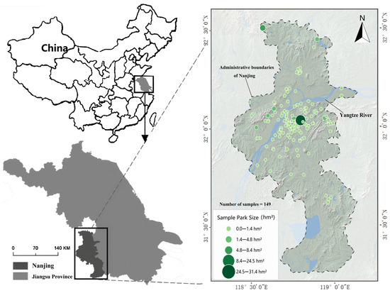
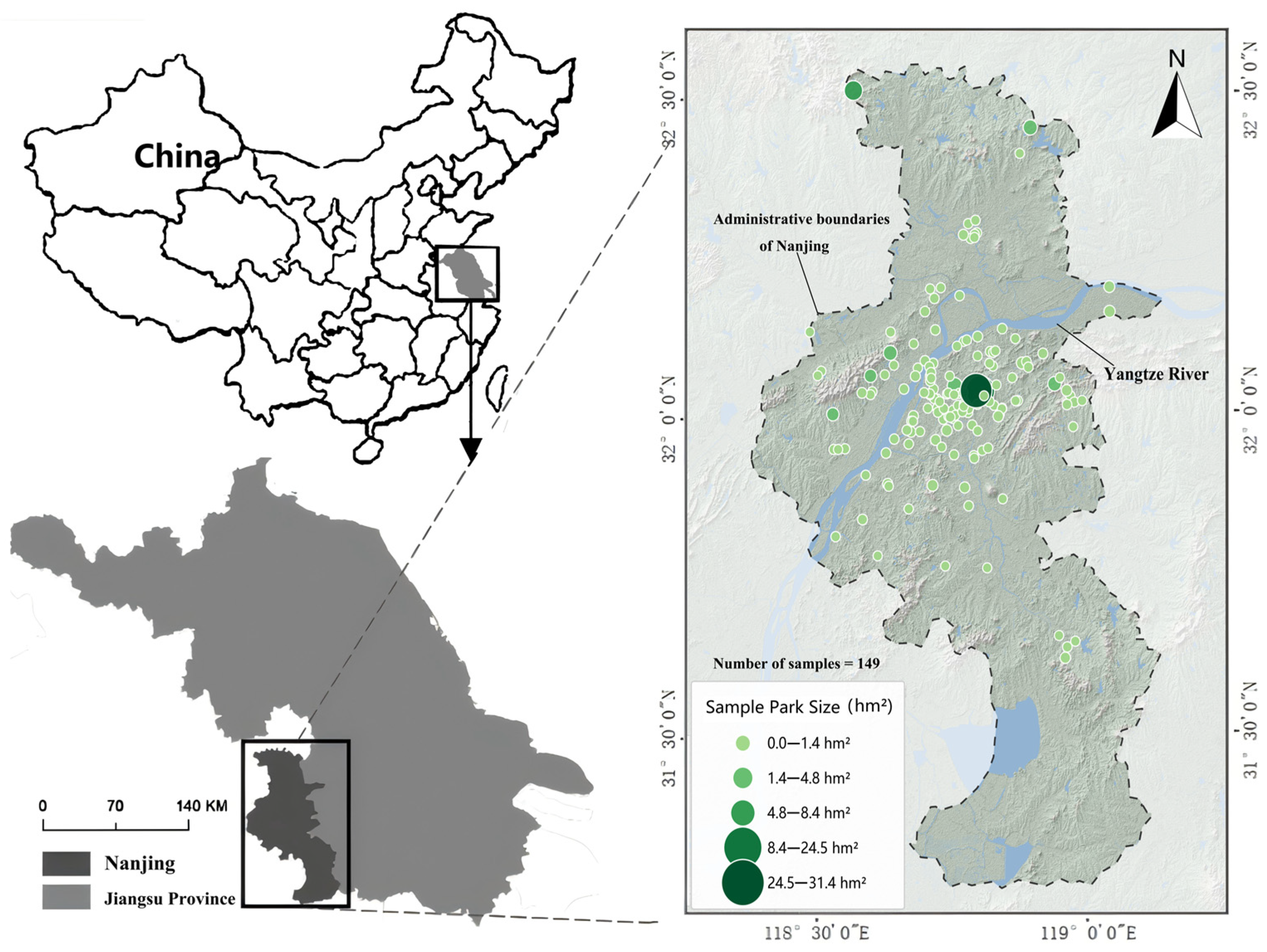
According to municipal statistics, the main urban area of Nanjing contains over 250 registered urban parks and green spaces of various sizes (defined here as publicly accessible green spaces providing ecological and recreational functions). However, to ensure the scientific validity and representativeness of the spatial analysis, this study systematically filtered these spaces and selected a purposive sample of 149 typical urban parks (Figure 1) based on three rigorous criteria:
Figure 1.
Location and overview of study area.
- (1)
- Area threshold: The minimum park area must exceed 0.5 ha. This is critical to mitigate the severe mixed-pixel noise inherent in Sentinel-2 10 m resolution data within highly fragmented high-density built environments;
- (2)
- Typological diversity: The sample must explicitly encompass various scale categories—specifically defined as pocket parks (0.5–2 ha), community parks (2–10 ha), comprehensive parks (10–50 ha), and large scenic forests (>50 ha)—to represent the urban green space system. Crucially, all these diverse park types were treated equally as independent spatial analysis units in the modeling process;
- (3)
- Data availability: The selected parks must possess clear municipal planning boundaries (initially obtained from the planning bureau and manually verified via high-resolution Google Earth imagery) and lack massive internal water bodies that would severely skew the vegetation-based ACFR estimation.
2.2. Data Acquisition and Processing
This study constructed a multi-source dataset comprising optical remote sensing imagery, topographic data, and vector boundaries (Table 1).
Table 1.
Data types and sources.
2.2.1. High-Resolution Remote Sensing Data Processing
Sentinel-2 MSI Level-2A imagery was selected, filtering for images with less than 5% cloud cover during the 2024 growing season (June to September) to minimize phenological noise [15]. Cloud removal and atmospheric correction were performed using the Sen2Cor algorithm on the Google Earth Engine (GEE) platform [16]. The red-edge bands (B5, B6, B7) with a 20 m resolution were resampled to 10 m to match the visible light bands [17]. Compared to Landsat, the 10 m resolution and unique red-edge bands of Sentinel-2 can more accurately retrieve the vegetation leaf area index and chlorophyll content [18]. The native 10 m Band 4 (Red) and Band 8 (NIR), which are sensitive to vegetation, were selected to calculate vegetation indices. For Band 5 (Red Edge 1, native 20 m), primarily used for calculating red-edge indices, it was uniformly resampled to a 10 m resolution using bilinear interpolation in GEE to construct a spatially consistent high-resolution feature set.
2.2.2. Carbon Sink Baseline Data
The CASA model, based on the light use efficiency principle, was employed to estimate net primary productivity [19]. Meteorological driving data, including monthly mean temperature, precipitation, and total solar radiation, were acquired from the National Meteorological Information Center of China and spatially interpolated to match the resolution of the remote sensing imagery. The model formula is as follows:
where APAR is the absorbed photosynthetically active radiation, and ε is the actual light use efficiency. Based on the pixel-scale NPP (g C/m2·yr), the total annual carbon fixation of each park was calculated through regional integration. To eliminate the scale effect caused by differences in park areas, this study set the Annual Carbon Fixation Rate (ACFR) as the target variable, standardizing it to units of t C/hm2/yr. It is crucial to clarify that ACFR in this study specifically refers to the area-normalized annual NPP-based vegetation productivity, rather than standing carbon density (stock) or net ecosystem carbon sequestration. As an urban ecosystem metric, it focuses on gross vegetation carbon fixation and does not account for heterotrophic respiration, soil decomposition, or management-related carbon losses (e.g., pruning, mowing, and litter removal). This temporally explicit flux definition strictly aligns with carbon balance measurement standards [20,21] while avoiding terminological conflation with long-term carbon storage.
NPP(x,t) = APAR(x,t) × ε(x,t)
2.2.3. Topographic Data
SRTM DEM data (30 m spatial resolution, preprocessed with void-filling and geometric calibration) was utilized to extract the digital elevation model and calculate slope, aspect, and the topographic wetness index (TWI). Given the highly fragmented nature of urban green spaces, the number of DEM pixels representing each park polygon varied significantly, ranging from 1–2 pixels for the smallest pocket parks to over a thousand pixels for large peripheral comprehensive parks. To reliably aggregate these topographic variables within the fragmented polygons, zonal statistics were calculated using the median value to represent the general topographic baseline of each park, thereby mitigating the influence of extreme edge pixels. Furthermore, because aspect is a circular variable (0–360°), direct arithmetic averaging is mathematically invalid (e.g., averaging 355° and 5° yields an incorrect southern exposure of 180°). Therefore, pixel-level aspect values were first converted into sine and cosine components, spatially aggregated via the median, and then back-transformed using the arctangent function to correctly determine the predominant exposure for each park unit.
2.2.4. Feature Variable System
To comprehensively analyze the driving mechanisms of the urban park Annual Carbon Fixation Rate (ACFR), this study constructed a feature variable system encompassing three dimensions: “ecological supply–spatial morphology–environmental constraints” (Table 2) [21]. Within the ecological supply dimension, indicators including LAI, FVC, and NDVI were selected to represent the carbon sequestration potential, structural complexity, and physiological vitality of the vegetation community, acting as the core parameters for the photosynthetic interface [22]. The spatial morphological dimension utilizes the ISP and NDBI to quantify the intensity of human disturbance and gray infrastructure stress, while incorporating the shape index and patch perimeter to characterize boundary fragmentation and landscape edge effects [23]. The environmental constraint dimension reflects the microclimatic conditions of site habitats through elevation (DEM), slope, and the Topographic Wetness Index (TWI) [24,25]. In particular, to avoid the mathematical aggregation bias inherent in circular variables (0–360°), the original topographic aspect was trigonometrically decomposed into Northness and Eastness to accurately capture solar radiation and hydrothermal redistribution. This system effectively covers the dual impacts of natural baseline conditions and anthropogenic activities, providing multidimensional data support for subsequent nonlinear attribution analysis based on the Random Forest model.
Table 2.
Driving factor system of urban park Annual Carbon Fixation Rate.
2.3. Explainable Machine Learning Framework
2.3.1. Random Forest Model
Given the nonlinearity of urban ecological processes and the strong collinearity among multi-source variables [26], this study employed the RF algorithm to process high-dimensional collinear data, constructing a nonlinear fitting and attribution model for the Annual Carbon Fixation Rate. By aggregating the prediction results of multiple decision trees, this method partially overcomes the limitations of traditional linear models, which struggle to capture complex threshold responses and are easily disturbed by multicollinearity. The model was implemented and optimized based on the Python (version 3.9) scikit-learn (version 1.0) and pandas (version 1.4) libraries. To build the Random Forest model, the 149 sample parks were randomly partitioned into a training set (80%, n = 119) and an independent testing set (20%, n = 30). Hyperparameter tuning was systematically executed using the GridSearchCV algorithm. The optimized model utilized 500 decision trees (n_estimators = 500), a maximum tree depth of 15 (max_depth = 15), and the square root method for maximum features (max_features = ‘sqrt’). To prevent overfitting and quantify model uncertainty, standard 5-fold cross-validation was strictly applied during the training phase. Furthermore, because the sample units are spatially distributed urban parks, we acknowledge that inherent spatial dependence might inflate traditional model performance metrics. While traditional random K-fold cross-validation was employed here to ensure baseline stability, the lack of spatial cross-validation is explicitly recognized as a methodological limitation, which should be incorporated in future studies to fully decouple spatial autocorrelation.
Furthermore, to rigorously address potential collinearity between the CASA-derived target variable and certain vegetation indices, a robustness test employing Permutation Feature Importance was conducted by systematically excluding highly collinear predictors.
2.3.2. SHAP Attribution Analysis
To eliminate the opacity of machine learning models, this study introduced the SHAP algorithm, based on cooperative game theory, to construct an attribution analysis framework [14]. Implemented via the Python shap library, by calculating the marginal contribution of each feature to the prediction outcome, this algorithm can generate feature dependence plots, which are critical technical tools for identifying nonlinear thresholds. This study conducted analysis from three dimensions: (1) global importance: establishing the contribution hierarchy of driving factors based on the mean absolute SHAP values; (2) nonlinear responses: utilizing dependence plots to visualize the marginal effect curves of key factors and identify ecological thresholds; (3) interactive mechanisms: calculating feature interaction values to explore the joint driving effects of human disturbances and natural baseline factors, indicating the nonlinear coupling patterns in complex habitats [27,28]. Furthermore, to statistically validate the interactive mechanisms (i.e., ecological compensation effects) across different disturbance levels, an Analysis of Covariance (ANCOVA) with 95% confidence intervals was integrated to assess the significance of slope differences.
2.3.3. K-means Clustering for Park Classification
To translate predictive thresholds into actionable planning guidelines, the 149 sample parks were classified using the K-means clustering algorithm. Prior to clustering, the core driving variables identified by the model (ACFR, LAI, ISP, and NDBI) were Z-score standardized to eliminate dimensional biases. To rigorously justify the classification, alternative numbers of clusters (from K = 2 to 9) were systematically tested and cluster stability was assessed. Based on the Within-Cluster Sum of Squares (WCSS) from the Elbow method and the Silhouette Score analysis (Supplementary Figure S2), three clusters (K = 3) were ultimately selected. Although K = 2 yielded a mathematically higher Silhouette coefficient, K = 3 was identified as the optimal inflection point that perfectly balances high intra-cluster similarity with sufficient typological granularity necessary for targeted urban planning interventions.
2.3.4. Technical Route
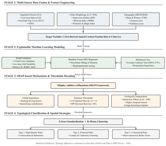
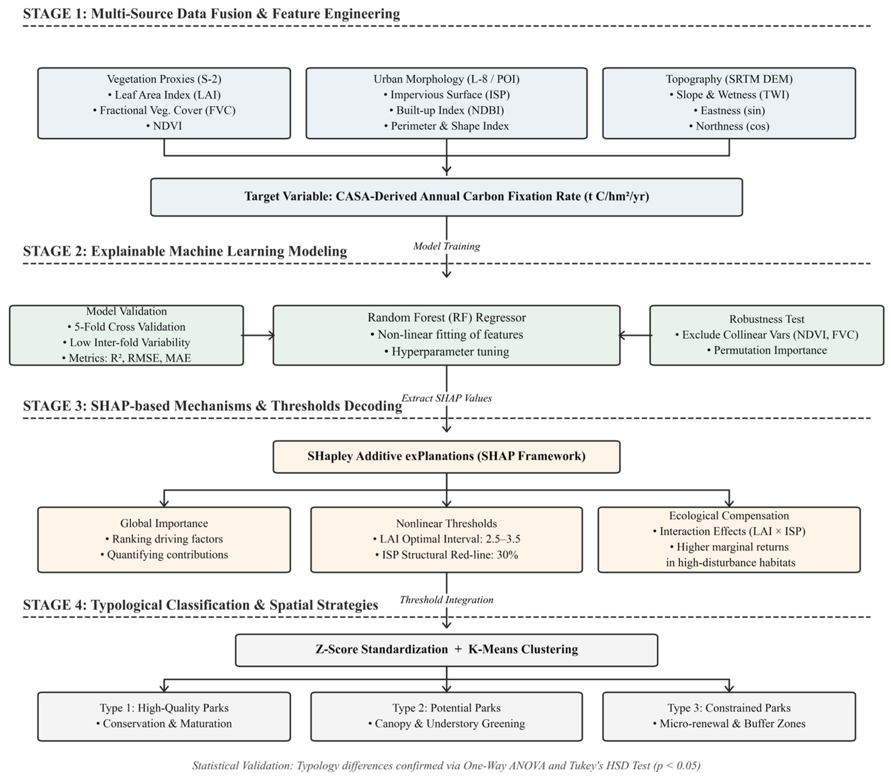
The methodological framework (Figure 2) was constructed to systematically bridge the research gaps identified through the literature review in Section 1.2, specifically the inability of traditional linear models to capture ecological thresholds and the “black-box” nature of advanced machine learning algorithms. To achieve the overarching aim of this study, the framework integrates data collection, model simulation, interpretation, and spatial validation into a cohesive workflow.
Figure 2.
Technical flowchart of study.
First, regarding data collection, high-resolution spatial datasets (Sentinel-2 MSI, SRTM DEM, and ESA WorldCover) were acquired from public repositories to accurately capture the fragmented micro-habitats of urban parks. The CASA model was utilized to calculate the Annual Carbon Fixation Rate (ACFR) as the target variable.
Second, the Random Forest (RF) algorithm was employed because of its robust capacity to process the severe high-dimensional collinearity inherent in urban ecological variables. Subsequently, the SHAP framework was introduced as a crucial explanatory tool. This specific combination is highly appropriate for this study, as it attempts to translate the algorithm’s complex nonlinear outputs into quantifiable ecological thresholds and compensation mechanisms.
Finally, the findings were refined and spatially validated through K-means clustering to propose actionable planning guidelines. The predictive reliability of the entire workflow was strictly validated using 5-fold cross-validation and standard statistical evaluation metrics (R2, RMSE, MAE).
3. Results and Analysis
3.1. Spatial Differentiation of Carbon Sink Efficiency and Model Applicability
3.1.1. Geospatial Mapping and Differentiation Patterns of the Multidimensional “Ecology–Morphology–Environment” Driving Factor System
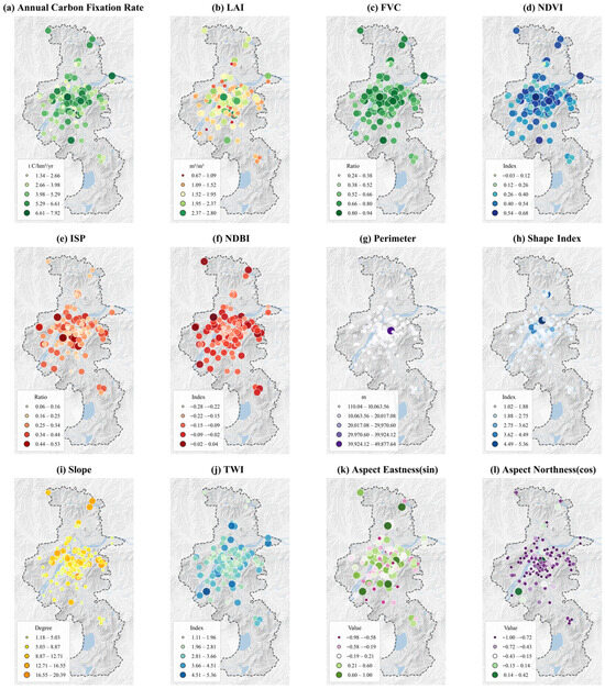
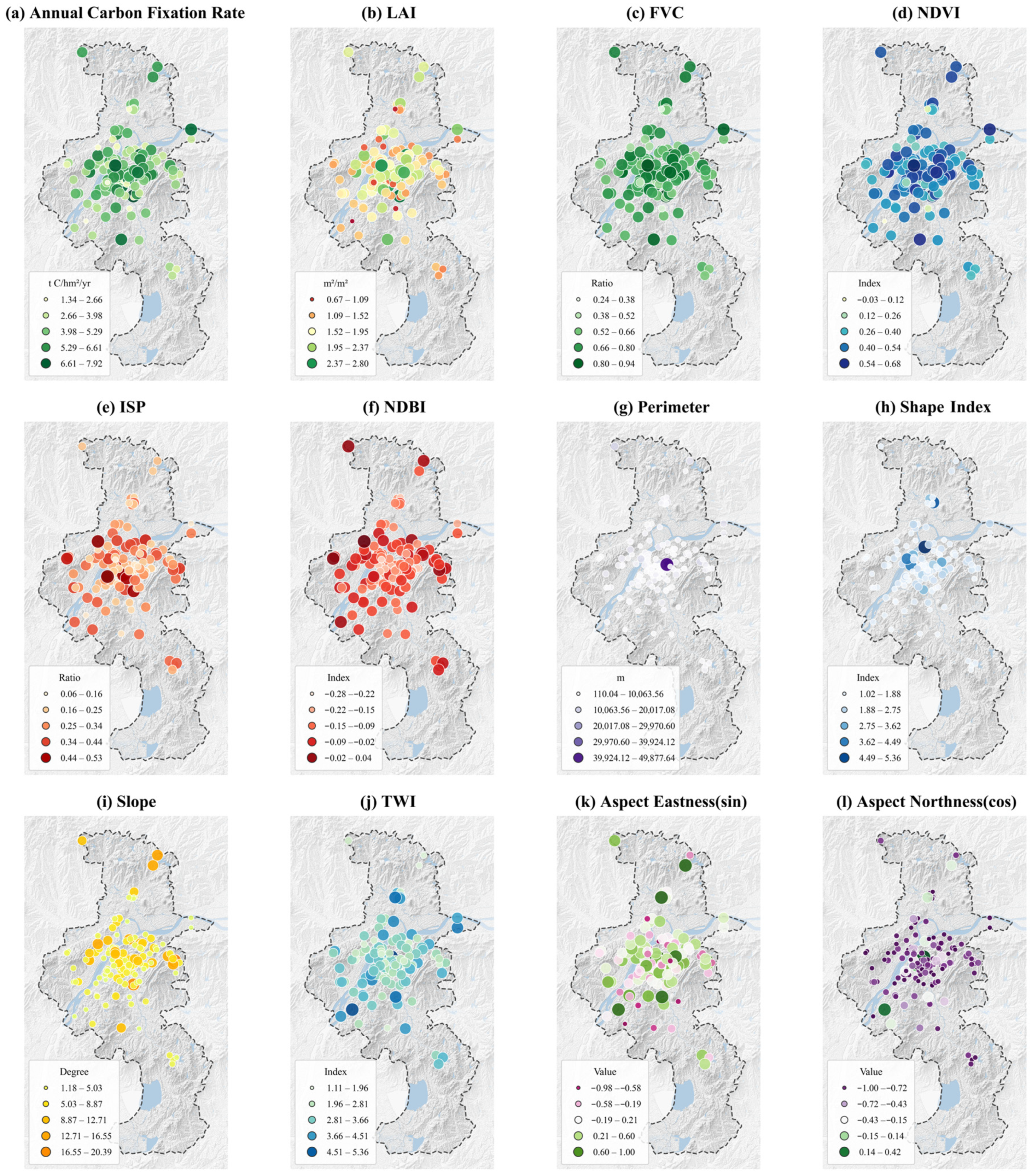
To intuitively visualize the spatial heterogeneity of urban park carbon sink efficiency and its potential influencing factors, this study conducted a spatial visualization of the target variable (ACFR) and 10 representative driving factors for the 149 sample parks in Nanjing (Figure 3). Note that while elevation (DEM) is a crucial environmental constraint in the modeling process, it is omitted from this 3 × 4 visual matrix for layout brevity. Overall, these indicators exhibit a complex spatial mosaic pattern. While large peripheral parks generally maintain higher carbon efficiencies, several well-maintained core urban parks also exhibit relatively high values, refuting a simplistic “center–periphery” gradient and highlighting the heterogeneous nature of urban green infrastructure.
Figure 3.
A spatial distribution matrix of the Annual Carbon Fixation Rate (ACFR) and multidimensional driving factors across the 149 sampled urban parks. Abbreviations: ACFR (Annual Carbon Fixation Rate); LAI (Leaf Area Index); FVC (Fractional Vegetation Cover); NDVI (Normalized Difference Vegetation Index); ISP (Impervious Surface Percentage); NDBI (Normalized Difference Built-up Index); TWI (Topographic Wetness Index). Note: To avert aggregation bias inherent in circular variables, the topographic aspect was trigonometrically decomposed into Aspect Eastness (sin) and Aspect Northness (cos).
- (1)
- Spatial synergy between ACFR and the ecological supply dimension: As shown in Figure 3a, the Annual Carbon Fixation Rate (ACFR) of urban parks presents a complex, heterogeneous mosaic distribution rather than a simplistic distance–decay gradient. While several peripheral parks exhibit high ACFR, notable high-value hotspots are also embedded within or adjacent to the urban core (e.g., large comprehensive scenic areas), whereas some peripheral areas in the south display relatively low values. The spatial patterns of the three indicators in the ecological supply dimension—Leaf Area Index (Figure 3b), Fractional Vegetation Cover (Figure 3c), and Normalized Difference Vegetation Index (Figure 3d)—exhibit a high degree of synergistic consistency with ACFR. This indicates that physiological vitality and canopy structure, rather than mere geographical location, dictate carbon sink efficiency.
- (2)
- Spatial morphological dimension: In the spatial morphological dimension (Figure 3e–h), the Impervious Surface Percentage (Figure 3e) and the Normalized Difference Built-up Index (Figure 3f) present a prominent mono-centric clustering pattern of “high in the core, low at the edge,” indicating that parks in the central area face intense hard boundary stress. However, in terms of patch perimeter (Figure 3g) and shape index (Figure 3h), the distribution is highly variable. While many core-area micro-parks possess short boundaries and regular shapes, the presence of mega-parks within the urban matrix creates prominent high-value outliers with complex geometric boundaries right near the geographical center. This morphological spatial heterogeneity profoundly interferes with the ecological processes of carbon fixation.
- (3)
- Topographic and geomorphological imprints of the environmental constraint dimension: The indicators of the environmental constraint dimension (Figure 3i–l) clearly map the geographical imprints of Nanjing’s micro-topographic undulations. Specifically, the high-value points of topographic slope (Figure 3i) highly overlap with specific natural mountainous areas within and at the edge of the city. These areas are usually subject to less direct disturbance from human activities, and variations in the topographic wetness index (Figure 3j) and aspect exposures (Figure 3k,l, where aspect is trigonometrically decomposed into sine and cosine components) provide diverse habitat conditions for vegetation communities, constituting a topographic protection barrier to a certain extent.
In summary, the ACFR of urban parks in Nanjing is not randomly distributed; instead, it deeply intertwines and overlaps spatially with ecological, morphological, and topographic factors. This highly nonlinear and spatially heterogeneous characteristic indicates that traditional global linear regression models struggle to accurately capture the true driving mechanisms of various factors on ACFR. Therefore, introducing the Random Forest algorithm and the SHAP explanation framework, which can handle complex nonlinear mapping relationships, has significant scientific necessity.
3.1.2. Statistical Distribution and Spatial Differentiation Characteristics of Annual Carbon Fixation Rate
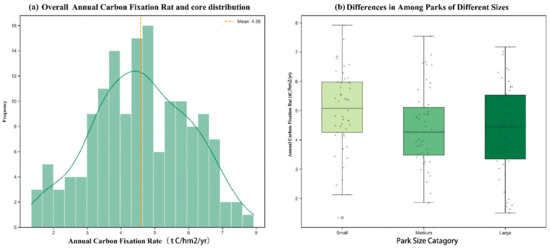
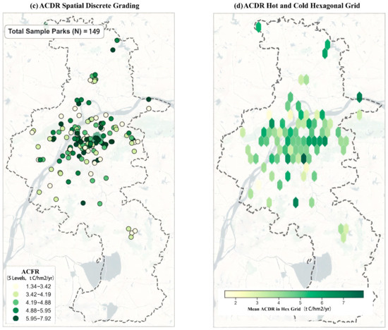
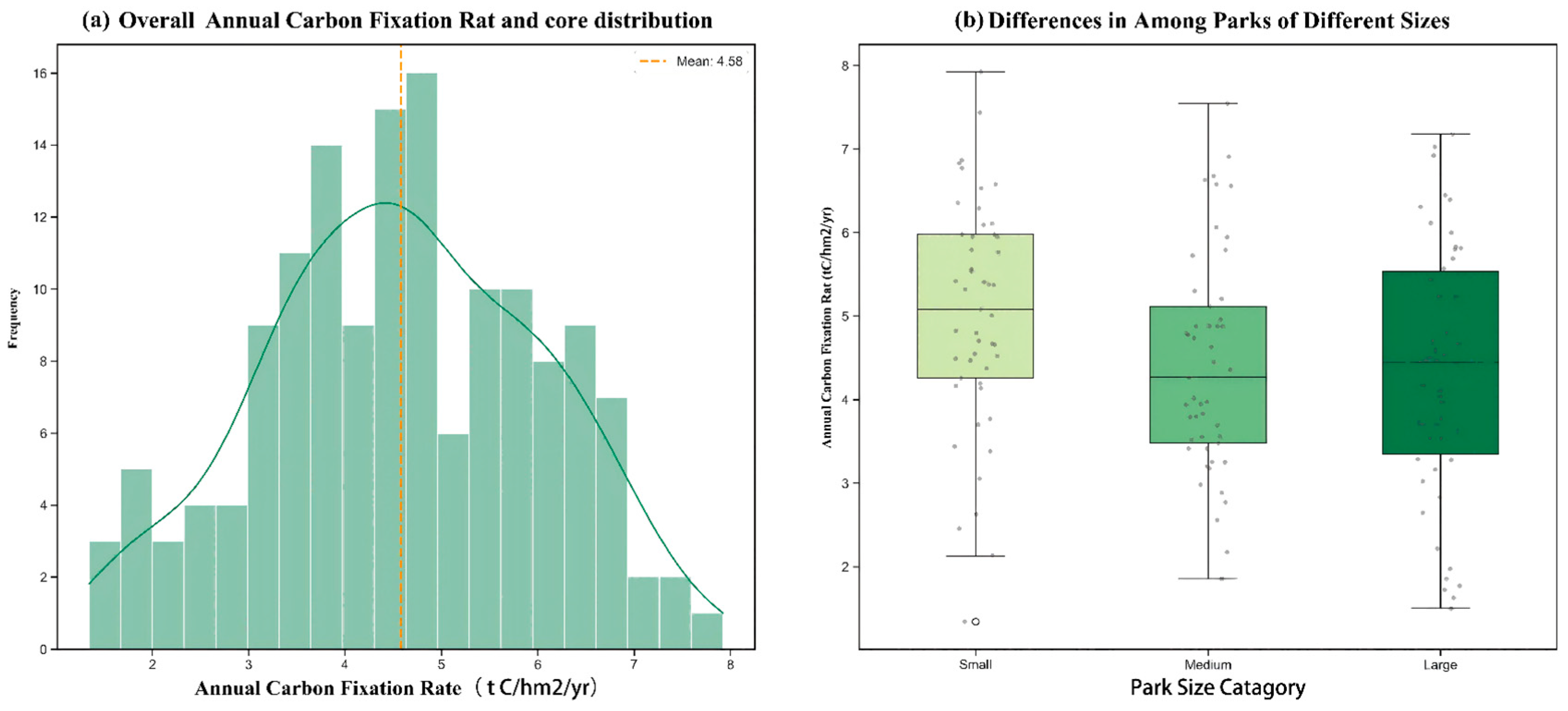
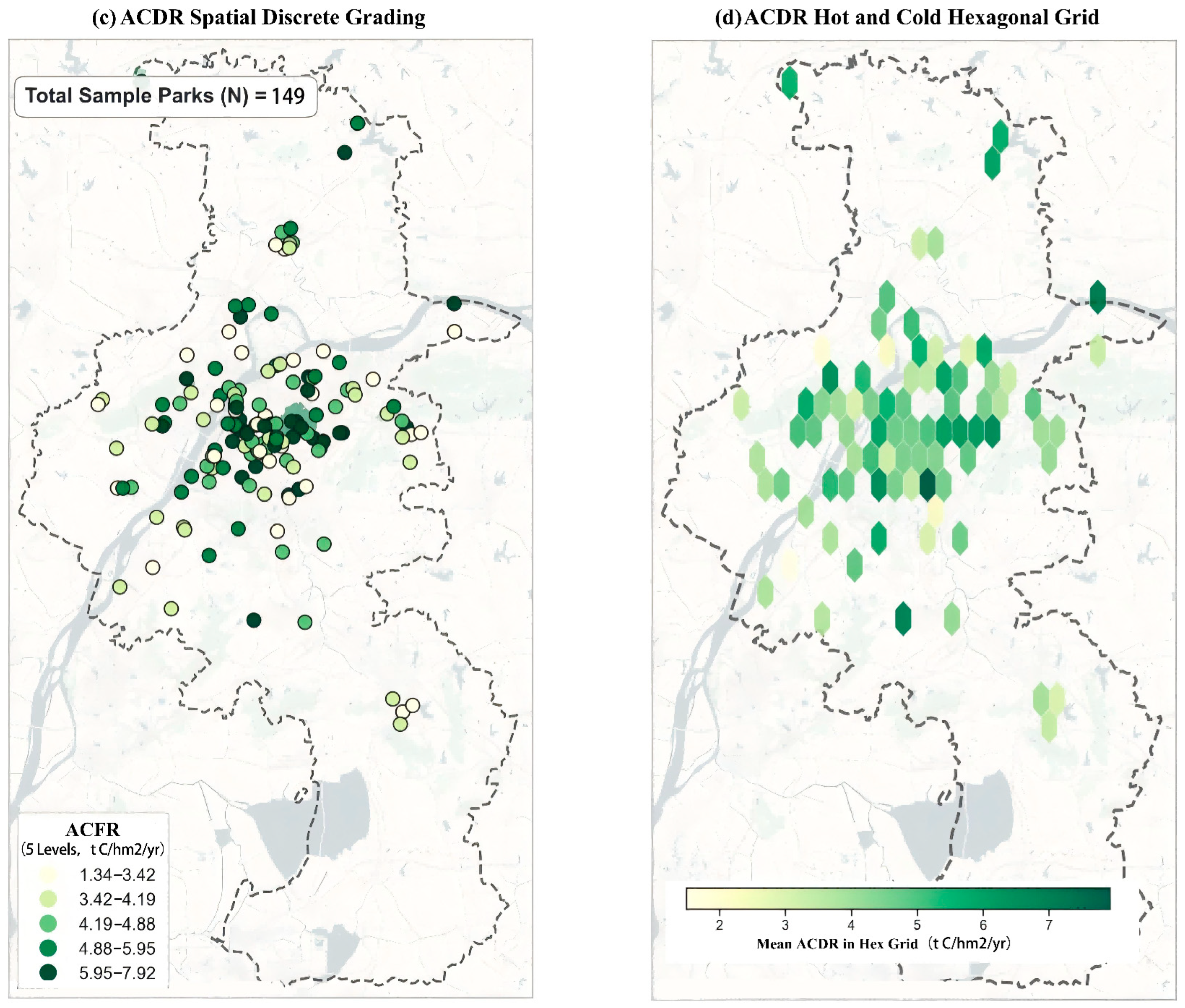
Accurately evaluating the baseline characteristics of existing urban park carbon sinks is a scientific prerequisite for formulating differentiated spatial renewal and optimization strategies. Breaking through the limitations of single-dimensional analysis, this study nested mathematical statistical patterns with geospatial mapping to construct a comprehensive analytical matrix from a dual statistical–spatial perspective (Figure 4).
Figure 4.
Comprehensive matrix of statistical characteristics and spatial differentiation of park Annual Carbon Fixation Rate.
- (1)
- Statistical Characteristics: The contrast between overall equilibrium and the high efficiency of micro-green spaces. In the statistical distribution dimension (Figure 4a), the mean Annual Carbon Fixation Rate of the 149 sample parks in the study area is 4.58 t C/hm2/yr, and its kernel density estimation curve presents an approximate normal distribution with a slight right-skewed tail. This indicates that the carbon sink supply efficiency of most urban parks tends toward a medium equilibrium state, while green patches with extremely high carbon sink levels are scarce resources in the urban matrix. Notably, the boxplot analysis based on the park spatial scale (Figure 4b) suggests an apparent descriptive scale–efficiency relationship. Contrary to the traditional assumption of increasing returns to scale, the median carbon density of small parks (approximately 5.1 t C/hm2/yr) and the overall data distribution center descriptively trends higher than those of medium and large parks. However, it should be noted that this high efficiency reflects model-derived potentials, which warrants future validation with field biometric measurements. The internal mechanism of this statistical contrast can be attributed to the heterogeneity of underlying surface composition: large municipal/comprehensive parks usually contain a large proportion of non-vegetated underlying surfaces, leading to significant dilution of the average Annual Carbon Fixation Rate per unit area. In contrast, small community or pocket parks, constrained by space, mostly adopt a high-canopy-closure, multi-layered plant community configuration mode, thereby maximizing spatial carbon sink efficiency at the local micro-scale [29]. This finding provides strong quantitative evidence for high-density built-up areas, under stock land constraints, to enhance overall carbon sink efficiency through the spatial implantation and community structure optimization of micro-green spaces.
- (2)
- Spatial Patterns: High concentric agglomeration and local carbon sink hotspots. In the geospatial dimension, this study combined discrete point mapping (Figure 4c) with a hexagonal grid model (Figure 4d) to deeply analyze the spatial differentiation and agglomeration patterns of Annual Carbon Fixation Rate [30]. Figure 4c intuitively characterizes the actual geographical locations and carbon sink capacity tiers of the sample parks under the high-density built environment context using a 5-level quantile discrete classification. The results show that high-carbon-sink patches (5.95–7.92 t C/hm2/yr) are not entirely marginalized to the peripheral natural forest edges but exhibit obvious spot-like core mosaic characteristics. To effectively filter out spatial visual biases caused by individual park morphologies and boundary sizes, Figure 4d introduces a hexagonal grid to reconstruct the spatial carbon sink center of gravity. The dark green grid highlighted areas clearly outline the high-carbon-sink spatial agglomeration network in the central and eastern parts of Nanjing’s main urban area. This spatial evolution characteristic indicates that although the core urban area faces extremely high building and population density stress, relying on the mature green space matrix of historical remains and high-density vegetation communities, it still plays an irreplaceable carbon sink anchoring role in the macroscopic urban ecological framework. This is logically consistent with the high carbon sink efficiency demonstrated by small green spaces in the statistical dimension mentioned earlier.
In summary, the Annual Carbon Fixation Rate of urban parks in the study area exhibits statistically intensive high-output characteristics in micro-green spaces and spatially heterogeneous core-mosaic features. This profoundly indicates that facing the demands for carbon sink enhancement in highly urbanized areas, it is difficult to adopt homogenized large-scale expansion strategies. Instead, there is an urgent need to establish a spatial classification intervention framework coupling the natural baseline with multidimensional variables of the built environment to achieve targeted renewal and precise empowerment of the green space system.
3.1.3. Variable Collinearity Diagnosis and Model Fitting Performance
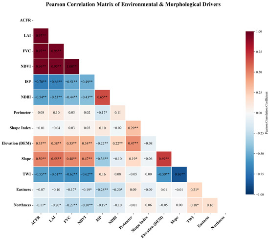
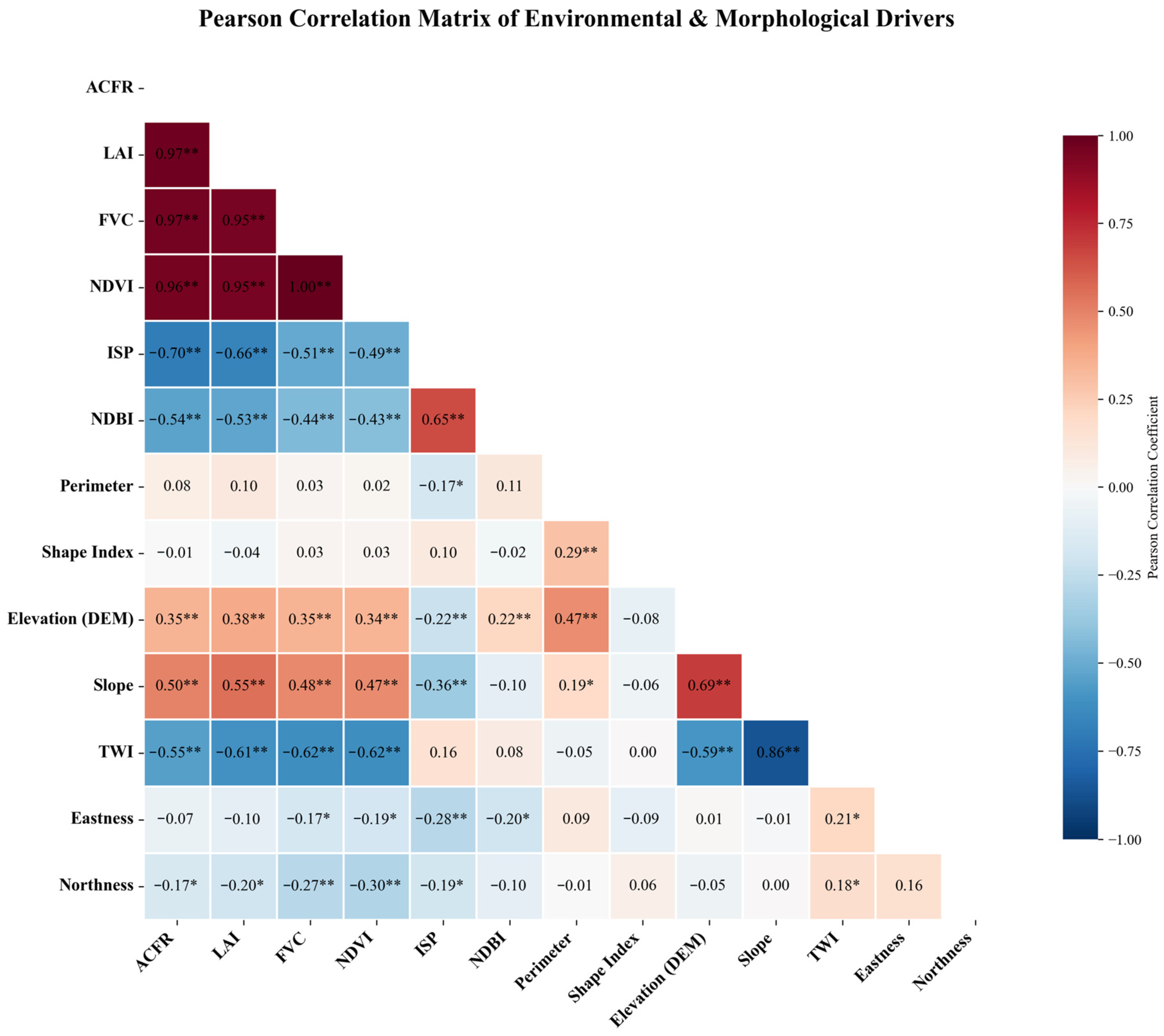
Pearson correlation analysis (Figure 5) reveals the widespread high-dimensional collinearity characteristics of urban ecological data. Especially among vegetation parameters, LAI and ACFR (r = 0.97) and NDVI and FVC (r = 1.00) all exhibit nearly perfect positive correlations. If traditional OLS regression were used, this multicollinearity would make it difficult for the model to distinguish the independent contributions of different vegetation indicators.
Figure 5.
Pearson correlation heatmap of driving factors. (Note: ** indicates significant correlation at the 0.01 level, and * indicates significant correlation at the 0.05 level.)
In contrast, the Random Forest regression model constructed in this study demonstrated excellent robustness owing to its feature random subspace mechanism. Accuracy validation based on the test set shows that the predicted values and measured values are closely distributed along the 1:1 line. The Random Forest model demonstrated robust predictive reliability in estimating the ACFR. During the training phase, the 5-fold cross-validation yielded a mean R2 of 0.952 with a standard deviation of ±0.018, indicating low variability and high stability across different data folds. The goodness of fit (R2) achieved was 0.9690. The Root Mean Square Error (RMSE) was 0.2494 t C/hm2/yr, and the Mean Absolute Error (MAE) was 0.1932 t C/hm2/yr. The consistency across these evaluation metrics supports the model’s accuracy and robustness in capturing the complex nonlinear relationships (Figure S3). This result also indicates that the model effectively learned and characterized the nonlinear patterns formed by the CASA model principles and environmental constraints, achieving a transition from extensive estimation to precise attribution.
3.2. Deconstruction of Driving Mechanisms: From Global Importance to Nonlinear Responses
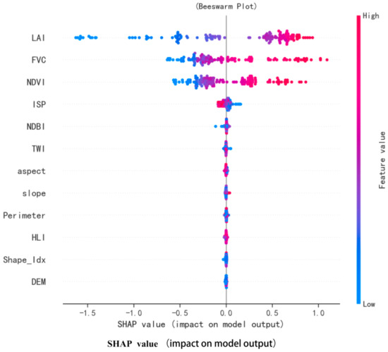
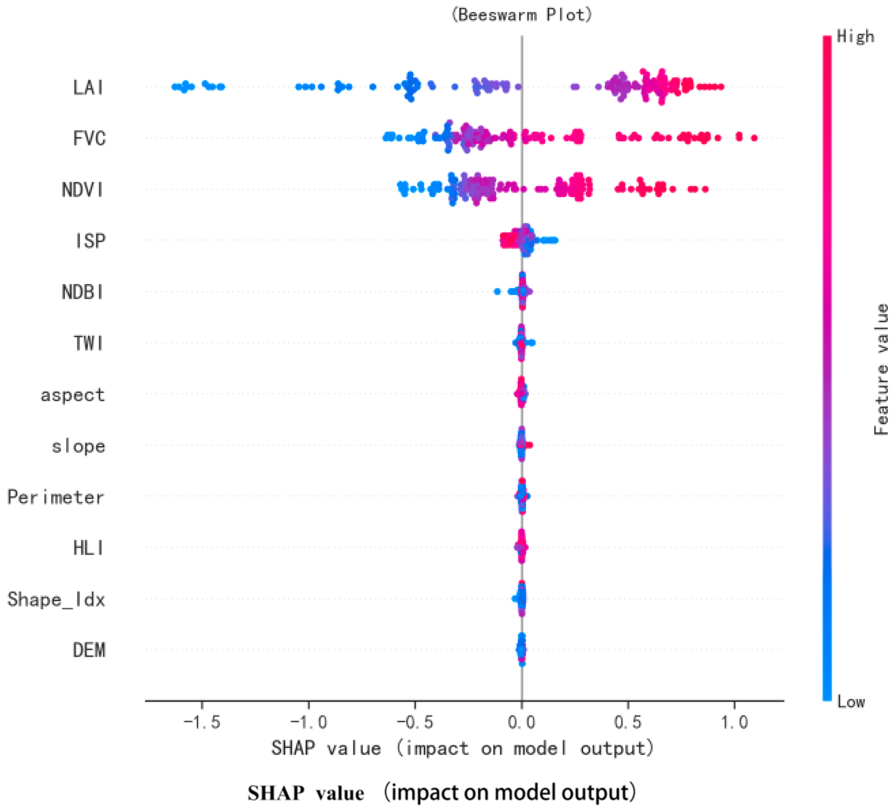
To deconstruct the internal mechanisms of the Random Forest model, this study utilized the SHAP algorithm to calculate the mean absolute contribution value of each feature and ranked their importance accordingly. Furthermore, the SHAP beeswarm plot (Figure 6) not only displays the feature importance ranking (top to bottom on the Y-axis) but also illustrates the model-derived positive or negative relationship between feature values and their impact on the Annual Carbon Fixation Rate. Red dots represent high feature values, and blue dots represent low values; a wider distribution of dots along the X-axis indicates a greater impact of that feature on the model output.
Figure 6.
SHAP beeswarm plot of driving factors.
The results indicate that the impacts of various driving dimensions on the Annual Carbon Fixation Rate present hierarchical differences:
- Dominant Layer: Vegetation structural parameters. It should be explicitly noted that the LAI, FVC, and NDVI are direct biophysical proxies of vegetation amount rather than external environmental drivers. Therefore, their high SHAP contributions primarily reflect the model’s reliance on variables definitionally linked to carbon fixation. The SHAP scatter for LAI has the widest distribution on the X-axis (−1.5 to 1.0), and the high values are concentrated in the positive region, indicating that it is the most influential model predictor of carbon sink levels. The FVC and NDVI follow closely, jointly constituting the material basis of carbon sinks. This highlights the potential ecological mechanism where three-dimensional green volume outperforms two-dimensional coverage; namely, under the same fractional vegetation cover, the vertical complexity of the canopy structure directly determines the effective light-receiving area for photosynthesis, thereby strongly influencing the upper limit of modeled carbon sequestration capacity.
- Limiting Layer: The red dots for ISP are strictly concentrated in the negative value region, and the blue dots are in the positive value region, with a clear demarcation, indicating a strong negative inhibitory effect. The expansion of hard paving not only directly erodes the effective carbon sink space but also indirectly limits plant growth by exacerbating sensible heat fluxes and altering soil hydrothermal conditions. Additionally, the distinct color stratification in the scatters for DEM and other data highlights the potential constraints of topography on carbon sinks.
- Regulatory Layer: Landscape morphological indicators. The overall contributions of the landscape shape index and slope are relatively small. This indicates that in high-density built-up areas, the marginal contribution of altering park boundary shapes to improving the Annual Carbon Fixation Rate is limited and far less effective than directly optimizing community structures.
3.3. Nonlinear Response Mechanisms and Threshold Identification of Key Factors
Before detailing the specific nonlinear threshold responses, it is crucial to clarify the interpretive boundary of the explainable machine learning framework. SHAP values mathematically explain the predictive behavior of the trained Random Forest model and the marginal contributions of each feature. Therefore, the identified nonlinear relationships and specific turning points (thresholds) should be interpreted as providing model-based evidence for ecological relationships, rather than directly proving absolute ecological causality confirmed by controlled field experiments.
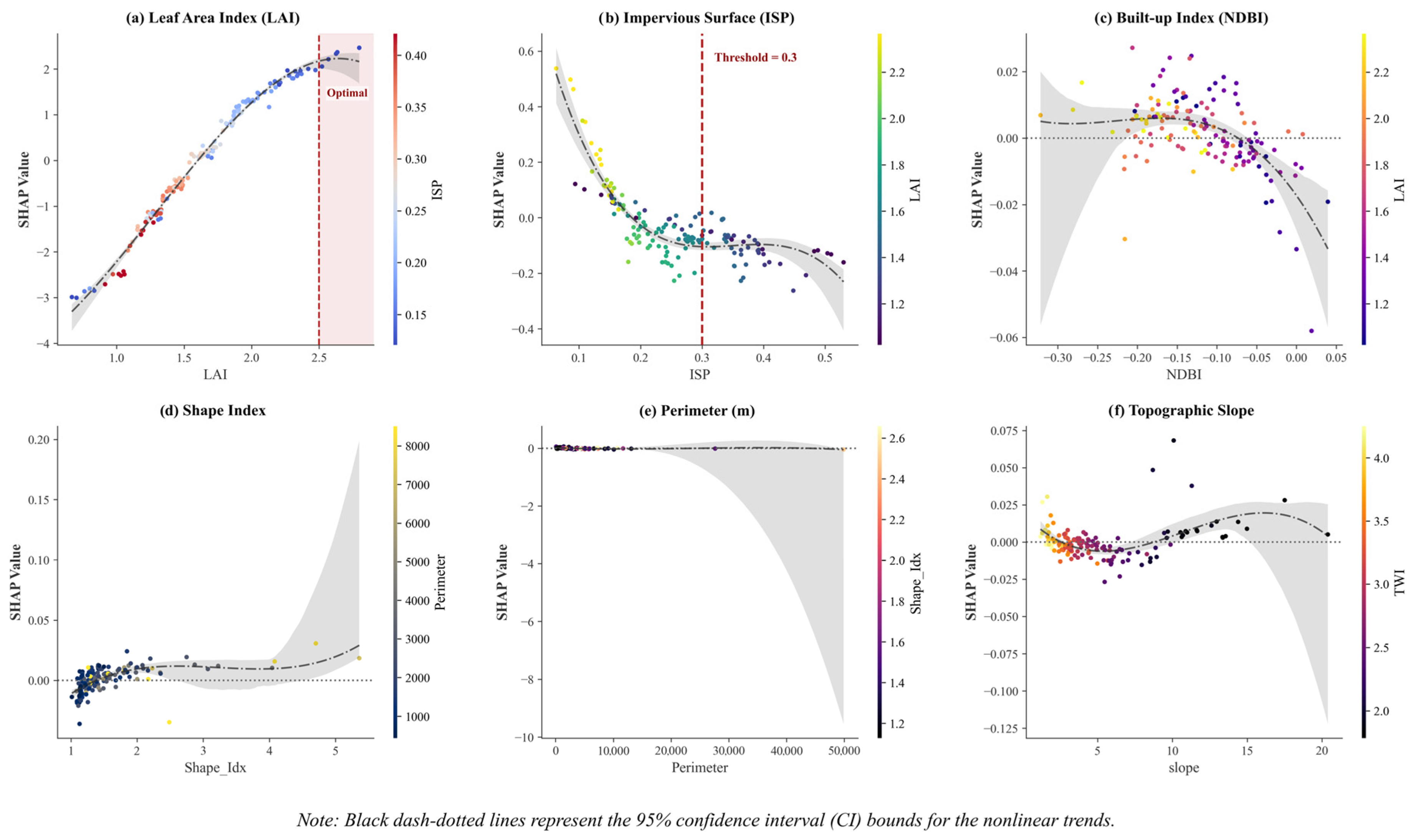
Although global importance ranking indicates the relative contribution weights of driving factors, it cannot depict the specific nonlinear response trajectories and marginal effects between the factors and Annual Carbon Fixation Rate. Given the complexity of urban ecosystems, single linear assumptions often obscure crucial ecological thresholds and saturation points. Therefore, based on SHAP dependence plots (Figure 7), this study further eliminated interactive interference among variables to analyze the independent nonlinear response trajectories of core variables from two dimensions—vegetation structural quality and habitat environmental constraints—to identify ecological thresholds and potential intervals indicative for urban green space planning.
Figure 7.
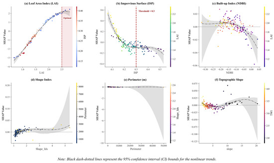
SHAP dependence plots of key driving factors with 95% confidence intervals. Note 1: (a) Leaf Area Index (LAI) showing a logarithmic growth trend, with the red dashed line indicating the potential optimal threshold; (b) Impervious Surface Percentage (ISP) indicating a rigid negative constraint with a critical ecological threshold at 0.3; (c) Normalized Difference Built-up Index (NDBI) displaying a localized single-peak trend; (d) Shape Index, (e) Perimeter, and (f) Topographic Slope exhibiting relatively flat marginal responses. Note 2: SHAP values and thresholds reflect the predictive behavior of the fitted Random Forest model, providing model-derived planning references rather than directly measured ecological causality. Note 3: Black dash–dotted lines represent the nonlinear fitted trends, while the gray shaded regions signify the 95% confidence interval (CI) bounds. The widening of the CI at the extreme ends of the feature values (e.g., large perimeters) visualizes increased predictive uncertainty due to sparse sample distributions.
3.3.1. Vegetation Structural Dimension: Quality Thresholds and Growth Potential
LAI: The trade-off between quasi-linear growth and optimal density interval. The SHAP dependence plot (Figure 7a) reveals an interesting phenomenon: within the observation range of the study area (LAI 0.7–2.8), the LAI and Annual Carbon Fixation Rate show a significant quasi-linear positive correlation, without the light saturation plateau commonly seen in natural forests. Mechanistically, this benefits from the unique edge effects of urban parks. Due to fragmented park patches and open edges, sunlight can penetrate the understory from the sides, effectively alleviating light competition within high-density communities. Therefore, even if the LAI is further increased, the lower-layer vegetation can still maintain high photosynthetic efficiency. This characteristic indicates that the current average LAI (1.65) of Nanjing’s urban parks has far from reached the critical point; elevating the LAI from the current mean of 1.65 to over 2.5 through the construction of multi-layered communities can still yield carbon sink increments without diminishing marginal returns. However, it is noteworthy that, according to predictive analysis, the entire LAI dependence curve exhibits a logarithmic growth characteristic—initially growing rapidly, then showing diminishing marginal returns, and finally tending toward saturation: Linear growth phase (LAI < 3.0): At this stage, the community has not yet closed, and increasing leaf area can significantly enhance light use efficiency, with SHAP values climbing linearly with LAI. Saturation plateau phase (LAI > 3.5): When the LAI exceeds 3.5, the slope of the curve approaches zero. This implies that an optimal density interval may exist at the planning level, namely LAI ≈ 2.8–3.5. Within this interval, the input–output ratio is the highest; blindly pursuing excessively high-density multi-layered planting not only wastes saplings but may also weaken ecological benefits due to interspecific competition.
However, these interpretations must be treated with caution. Our observed LAI values primarily range between 0.7 and 2.8. Consequently, the predicted saturation plateau at LAI > 3.5 represents a model extrapolation rather than an empirically observed threshold. Furthermore, the quasi-linear growth phase might partially reflect mixed-pixel effects (varying proportions of canopy and hardscape within a 10 m pixel) rather than purely physiological edge effects.
3.3.2. Habitat Environmental Dimension: Hard Paving Stress and Micro-Environment Regulation
The rigid constraint of ISP. The study found that 30% is a significant ecological critical point [30]. The dependence plot (Figure 7b) shows that the negative stress of impervious surfaces on Annual Carbon Fixation Rate presents a nonlinear phase transition characteristic: in the low-disturbance interval of 20%, the ecosystem can still maintain carbon sink resilience by preserving landscape connectivity; however, once the ISP breaches the critical point of 30%, the SHAP value drops precipitously. This phenomenon verifies the percolation threshold theory in landscape ecology, indicating that excessively high matrix resistance leads to the structural blockage of energy and material flows and the decline of system functions. Therefore, an ISP of 30% can serve as a reference control indicator for determining the maintenance of ecological integrity in urban park construction.
The single-peak hypothesis of the NDBI. The study found that the response curve of the NDBI (Figure 7c) presents a localized single-peak shape, with its peak appearing around −0.1. This peak may primarily reflect the compositional characteristics of mixed pixels containing specific proportions of vegetation and impervious surfaces at the 10 m spatial resolution. Although the “edge fertilization effect” or “moderate urban heat island promotion” proposed by existing studies offers a plausible ecological perspective, in the absence of supporting field flux or phenological data, this interpretation must be cautiously treated as a potential hypothesis rather than a confirmed mechanism.
Conversely, the dependence curves for morphological and topographic constraints, such as Shape Index (Figure 7d), Perimeter (Figure 7e), and Topographic Slope (Figure 7f), remain predominantly flat with relatively low SHAP value fluctuations. Notably, the 95% confidence intervals (gray shaded areas) expand significantly at the extreme high values for these variables, reflecting high predictive uncertainty due to data sparsity at the tails. This visually confirms their secondary and regulatory roles compared to the dominant constraints of the LAI and ISP.
3.4. Ecological Compensation Effects Under High-Disturbance Habitats
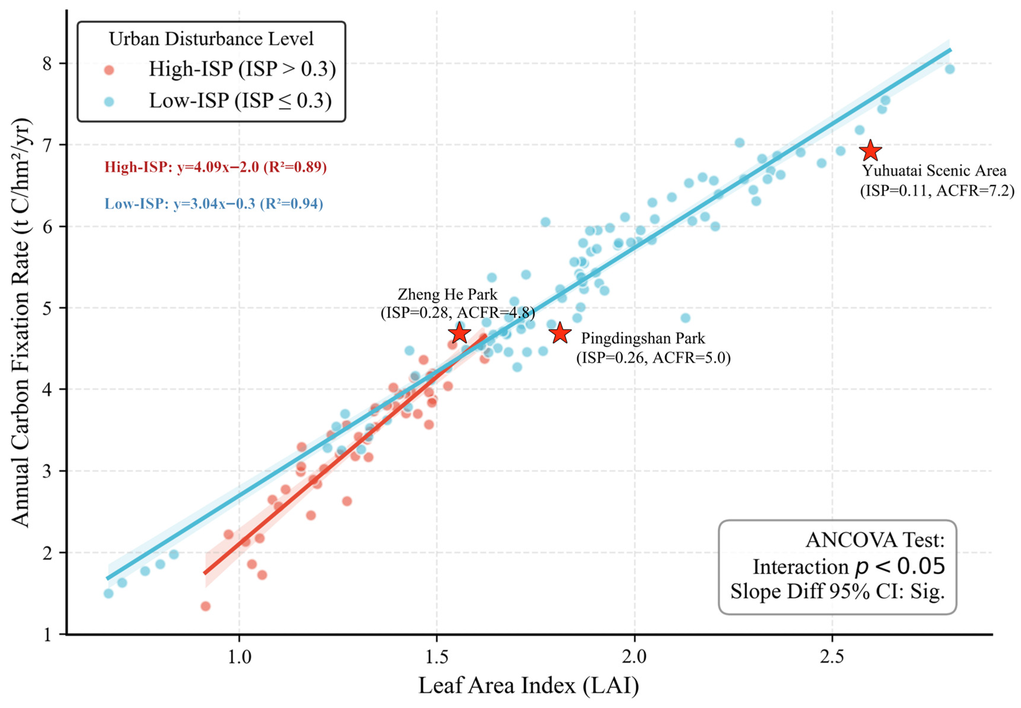
To explore the carbon sequestration performance of vegetation under different anthropogenic disturbance intensities, the study divided the parks into a high-disturbance group (High-ISP) and a low-disturbance group (Low-ISP) based on ISP values for interactive analysis (Figure 8). The regression analysis results show that in the high-disturbance group (High-ISP, red fitting line), the slope of the LAI enhancing the annual carbon fixation rate (ACFR) is 4.09 (R2 = 0.89), which is notably steeper than the slope of 3.04 (R2 = 0.94) in the low-disturbance group. To rigorously validate this observed divergence as an ecological compensation effect, an Analysis of Covariance (ANCOVA) was conducted. The statistical results confirmed a significant interaction between the LAI and ISP groups (p < 0.05), and the non-overlapping 95% confidence intervals clearly demonstrate the robust difference in slopes. This phenomenon reflects a potential ecological compensation effect [31,32]: in stressful environments such as high-density built-up areas, the comprehensive marginal ecological benefits of vegetation in improving microclimates and mitigating heat islands may be amplified. Taking Pingdingshan Park and Zhenghe Park as examples, although both are severely squeezed by surrounding high-density buildings and hard paving (ISP > 26%) and belong to typical high-disturbance habitats, by maintaining a high community canopy closure (LAI > 1.6), their annual carbon fixation rate still reached approximately 4.9 t C/hm2/yr, significantly higher than the mean of similar parks. This indicates that in central urban areas where land is at a premium, implementing micro-greening interventions yields a relative marginal ecological benefit in improving the living environment and enhancing carbon sinks that is higher than an equal scale of investment in suburban parks with good ecological baselines. This finding contradicts the traditional cognition that greening is inefficient in severely degraded environments and provides a degree of scientific basis for micro-renewal in historic urban cores: the more crowded the place, the higher the greening returns.
Figure 8.
Interactive relationship between LAI and annual carbon fixation rate (ACFR) under different disturbance habitats (Note: interaction effects and ecological compensation mechanisms reflect model-derived trends and potential biophysical associations).
3.5. Planning Guidelines: Typological Classification of Parks Based on Carbon Sink Efficiency and Result Validation
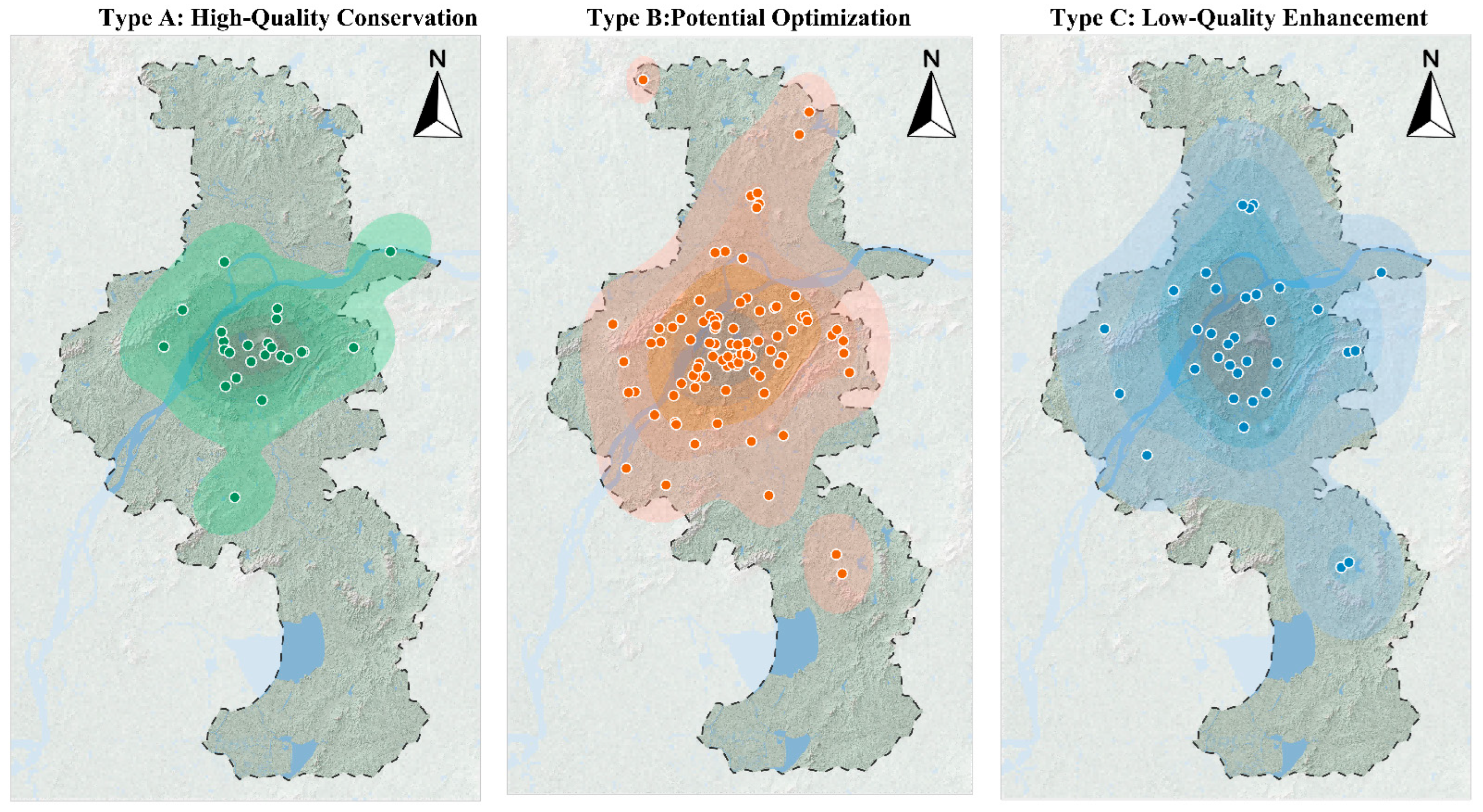
Based on the K-means clustering algorithm, this study classified the 149 urban parks into three typical modes (Figure 9) according to their carbon sink efficiency and core driving factors, aiming to achieve the translation from mechanism analysis to classified management (Table 3).
Figure 9.
Distribution and Clustering Characteristics of Three Types of Park Spaces.
Table 3.
Carbon Sink Efficiency Classification Table.
3.5.1. Type A: High-Quality Conservation Features
A high average Annual Carbon Fixation Rate (6.43 t C/hm2/yr), superior habitat quality, mostly distributed in the hilly areas around Purple Mountain and Laoshan. Typical representatives include Dongshan Park and Bazishan Park. These parks are the core carbon pools of the city. Strict conservation strategies should be adopted, ecological protection red lines should be delineated, and new construction land and excessive commercial development must be strictly prohibited, focusing primarily on maintaining their habitat authenticity.
3.5.2. Type B: Potential Optimization Features
All indicators are at median levels (Annual Carbon Fixation Rate 4.81 t C/hm2/yr); they are mostly comprehensive parks with complete facilities, possessing a certain amount of green volume, but the community structure still has room for optimization, such as Chaotian Palace and Nanjing Sculpture Park. These parks are the primary potential areas for carbon sink enhancement. It is recommended to adjust the community structure, introduce high-carbon-sequestration tree species, and increase the understory shrub and grass layers to elevate the LAI to the optimal interval of 3.0–3.5, achieving stock efficiency enhancement.
3.5.3. Type C: Low-Quality Enhancement Features
A low Annual Carbon Fixation Rate (3.13 t C/hm2/yr), high degree of hardening (ISP > 35%), mostly small-area, densely populated community pocket parks or squares, such as Kangyeli Park and Tianyin Park. These parks are severely constrained by hard spatial limits. Three-dimensional micro-renewal strategies should be adopted, utilizing vertical greening, roof greening, and permeable paving transformations to maximize the green view rate within limited space, leveraging their high marginal benefits to improve local micro-environments.
3.5.4. Validation of Classification Results Effectiveness
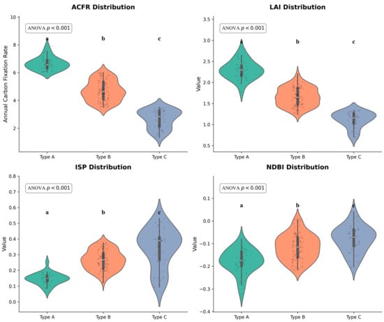
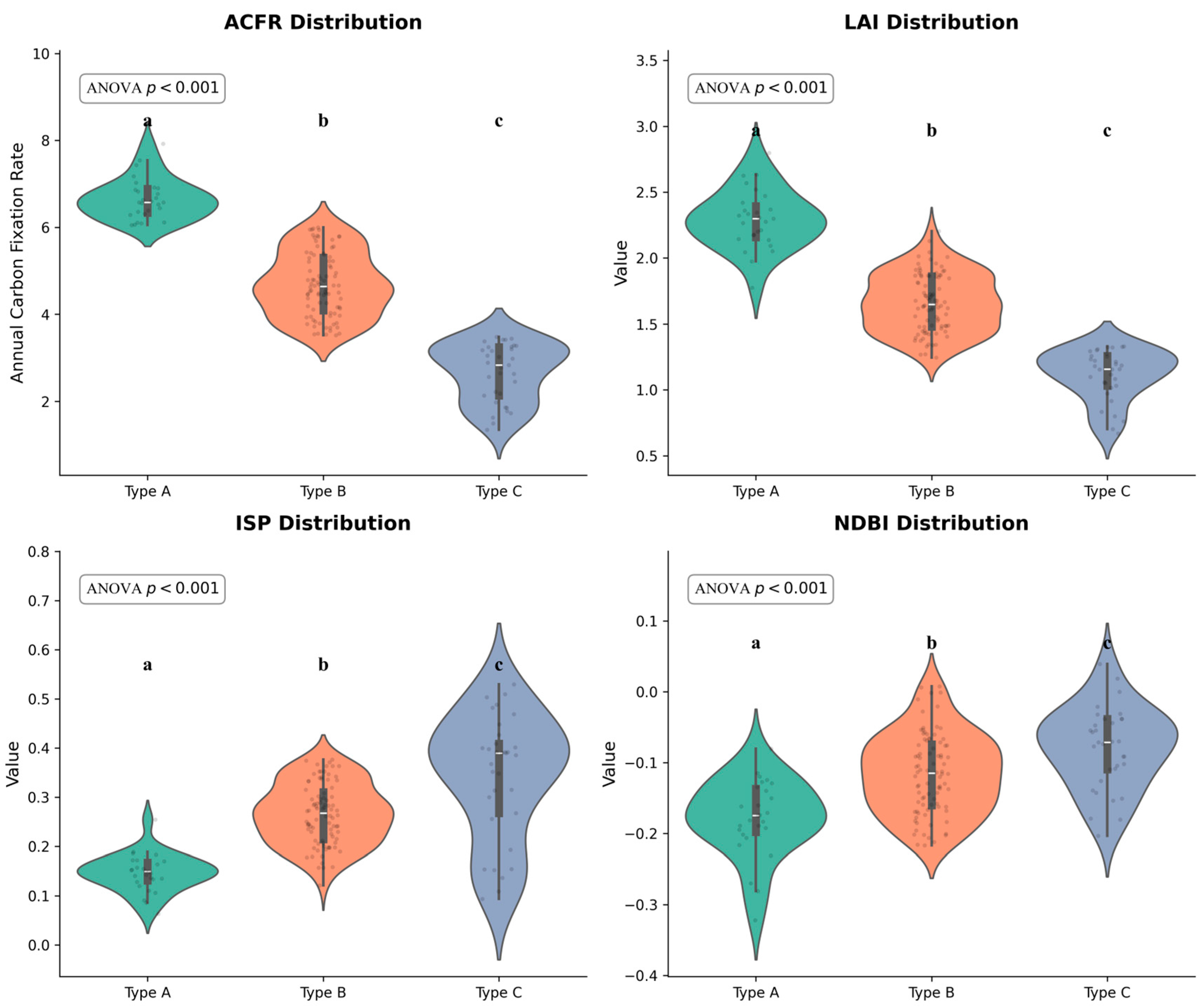
To further analyze the internal driving factors and environmental backgrounds of the three planning strategy zones, this study utilized violin plots to conduct a feature distribution comparison. Following the principle of highlighting the most critical driving mechanisms, the main text exclusively presents the four core variables (ACFR, LAI, ISP, and NDBI) that decisively define the typological boundaries (Figure 10). Furthermore, a one-way ANOVA with post hoc tests was conducted. The results indicated statistically significant differences (p < 0.001) across the three park types for these core variables, robustly validating the scientific rationality of the spatial classification. Detailed distributions for the remaining secondary variables are provided in Supplementary Figure S4.
Figure 10.
Multidimensional environmental feature analysis of the core variables across different planning strategy zones. Note: The violin plots illustrate the probability density and internal box plots (median and interquartile range) for the four primary driving factors: ACFR, LAI, ISP, and NDBI. Different lowercase letters (a–c) indicate statistically significant differences between park types based on a one-way ANOVA and subsequent post hoc tests (p < 0.001). Detailed distributions for the remaining secondary variables are provided in Supplementary Figure S4.
Synthesizing the multidimensional environmental feature distribution results indicates that the three types of planning strategy parks exhibit highly gradient differentiation and spatial heterogeneity in terms of ecological baselines and artificial stress features. Among them, high-quality conservation parks often rely on higher elevations and complex topography; they are less disturbed by urbanization artifacts, and the surrounding building density and impervious surface ratios are at extremely low levels. Therefore, they retain the most robust ecological baseline, demonstrating significant high-value clustering characteristics in the Annual Carbon Fixation Rate, leaf area index, and fractional vegetation cover. In sharp contrast, low-quality enhancement parks exhibit typical high-density built environment stress characteristics, with their NDBI and ISP indicators presenting an obvious “top-heavy” high-value clustering shape, indicating that they are deeply surrounded by high-intensity urban gray infrastructure. Furthermore, restricted by small areas and relatively simple shape indices, the overall vegetation growth and carbon sink functions of these parks are generally at the bottom, urgently requiring them to become core targets for future spatial micro-renewal and structural optimization. In comparison, potential optimization parks act as a transitional form, with the medians of their various indicators generally falling between the former two. However, their violin plot distribution shapes are the broadest on multiple indicators such as perimeter and topographic wetness index, reflecting extremely strong internal heterogeneity. These parks are mostly distributed in the fringe zones of urban expansion or new urban areas, possessing the greatest functional enhancement elasticity and transformation space, making them key potential areas for urban green space carbon sink efficiency enhancement in the future.
In conclusion, the carbon sink capacity of urban parks is not only the result of natural vegetation growth but also the spatial projection of the mutual game between their surrounding built environments and topographic conditions. Therefore, subsequent planning interventions should not be limited solely to green planting within the parks but need to be placed within the overall urban matrix for differentiated coordination.
4. Discussion
4.1. Mechanisms of Carbon Sink Efficiency Differences in High-Density Areas
The higher marginal response under high-disturbance habitats observed in this study may seem counterintuitive but actually aligns with urban ecological mechanisms. One plausible mechanism is the potential heat island promotion effect; studies suggest that the urban heat island effect might prolong the growing season of vegetation, thereby increasing the duration of carbon accumulation [33]. Nevertheless, the urban heat island effect acts as a double-edged sword; while it extends phenology, it can simultaneously exacerbate drought stress and accelerate soil moisture depletion. A second hypothesized driver is the edge fertilization effect; parks embedded in the urban matrix receive finer artificial maintenance and are more likely to capture high concentrations of atmospheric CO2 and nitrogen deposition [34,35]. Conversely, artificial maintenance is bidirectional; intensive management such as litter removal, pruning, and mowing may actually reduce organic matter inputs to the soil and negatively affect overall carbon accumulation. This suggests that conducting micro-renewal in historic urban cores not only improves the living environment but also yields a higher return rate on the ACFR compared to suburban parks, possessing prominent ecological and environmental equity values. However, these remain potential ecological hypotheses in this context. The observed higher marginal responses, such as the NDBI single peak, may also partly reflect mixed land-cover composition within pixels rather than distinct ecological mechanisms. As management intensity, direct temperature anomalies, and direct carbon fluxes were not explicitly quantified in this study, these model-derived associations require rigorous future field validation.
4.2. Application of Threshold Indicators and Law of Diminishing Marginal Returns
Identifying ecological thresholds is a prerequisite for realizing refined urban regeneration. Traditional planning guidelines often use two-dimensional indicators such as the green space ratio. The 30% ISP threshold and the 2.5–3.5 LAI suitable interval extracted in this study should be regarded as preliminary model-derived planning references rather than as firm ecological red lines or universally applicable design standards. They translate abstract, providing references for refined management. The study found that the inhibition of carbon sink functions by impervious surfaces exhibits a significant phase transition characteristic: an ISP of 30% can serve as a reference for determining the critical point of urban green space ecosystem integrity, and exceeding this threshold will lead to a substantial decline in carbon sink functions. Meanwhile, the response curve between the LAI and Annual Carbon Fixation Rate presents a typical law of diminishing marginal returns. The saturation period appearing after the LAI exceeds 3.5 indicates the crowding costs caused by light competition and resource limitations in high-density cities [36,37]. This demonstrates that in central urban areas with severe land resource shortages, pursuing a moderately intensive model with an LAI of 2.5–3.5 aligns better with the principle of optimal input–output than blindly piling up high-density communities. Perhaps future urban green space designs should not blindly pursue large lawns or large areas of hard plazas, but rather seek the optimal solution for three-dimensional green volume within limited spaces.
4.3. Limitations and Future Prospects
A notable constraint is the potential circularity between the CASA-derived target variable and certain inputs like the NDVI and FVC. While we acknowledge this inherent limitation of remote sensing modeling, we conducted a rigorous permutation robustness test by excluding these collinear indices (Supplementary Figure S1). The results firmly demonstrate that even without them, the LAI and ISP consistently emerged as the dominant drivers, proving that our core morphological and structural findings are not mere artifacts of mathematical circularity.
Although the explainable framework constructed in this study effectively analyzes the driving mechanisms of carbon sinks, limitations remain: (1) The target variable ACFR is derived from CASA-simulated NPP; although localized corrections were made, subsequent multi-scale cross-validation combined with ground-measured data (e.g., eddy covariance flux tower monitoring networks) [38,39] is still needed. (2) The single-year summer imagery fails to fully reflect the dynamic impact of phenological fluctuations on interannual carbon sink accumulation. (3) The soil carbon pool has not yet been included; future research needs to combine airborne LiDAR and long-time-series ground-based soil monitoring networks [40] to construct a comprehensive landscape carbon flow coupling analysis model.
Furthermore, while the empirical data and specific numerical thresholds (e.g., the LAI interval of 2.5–3.5) extracted in this study are fundamentally model-derived reference values specific to the climatic and urban context of Nanjing, the overarching analytical framework possesses universal applicability. The “Multi-source Data–RF–SHAP” workflow provides a scalable, reproducible template for evaluating urban ACFR globally. While the exact tipping points may vary geographically, the methodological approach to uncovering nonlinear diminishing marginal returns and potential ecological compensation effects in degraded matrices offers a universal paradigm for urban ecological planning. Future validation across different climatic regions and urban forest types would further evaluate the transferability of the proposed framework.
5. Conclusions
Addressing the urgent needs of urban stock planning in high-density cities and the widespread limitations of linear estimations and the “black box” problems of ecological processes in existing urban carbon research, this study constructed a comprehensive analytical framework of “Multi-source Remote Sensing–Machine Learning–SHAP Attribution”. Through empirical analysis of the park system in the main urban area of Nanjing, the main conclusions are as follows:
Addressing the first research question regarding nonlinear mechanisms, the model indicated that ACFR is not controlled by a single factor but is the result of a nonlinear game between ecological potential and environmental constraints. The high-fidelity fitting of the Random Forest model effectively quantified the biophysical driving forces dominated by LAI and the urban matrix constraining forces dominated by ISP, indicating the restrictive nature of hard environments on carbon sink potential.
In response to the second research question, this study quantified preliminary model-derived reference thresholds. This study identified a 30% impervious surface proportion as a potential planning reference for maintaining functional stability; exceeding this value may lead to a structural decline in ACFR functions. Concurrently, it identified 2.5–3.5 as the optimal efficiency interval for the vegetation leaf area index, providing a reference basis for balancing ecological benefits and construction costs. These reported thresholds should be strictly interpreted as decision support references generated by the model rather than universal ecological thresholds.
Addressing the third research question, model-based evidence suggested a potential ecological compensation effect. This study indicates the compensatory response characteristics of vegetation under high-disturbance habitats, suggesting that improving green space quality in old urban areas with significant heat island effects yields a significantly higher marginal ACFR return than in low-disturbance areas. Based on this, the proposed graded control strategies of high-quality conservation, potential optimization, and low-quality enhancement provide scientific support for the classified governance and refined regulation of urban stock green spaces.
Despite these insights, this study acknowledges several exploratory limitations. First, the target variable (ACFR) is a CASA-derived remote sensing estimate, not an independently field-measured carbon sequestration value. Consequently, the identified thresholds (e.g., LAI 2.5–3.5; ISP 30%) and ecological compensation effects should be strictly interpreted as model-derived planning references rather than universal, empirically confirmed ecological rules. Future research must incorporate field-based biomass validation, soil carbon measurements, and cross-seasonal imagery to address potential spatial autocorrelation and overcome the limitations of single-year summer observations.
Supplementary Materials
The following supporting information can be downloaded at: https://www.mdpi.com/article/10.3390/f17070849/s1, Figure S1: Permutation feature importance and robustness test of the Random Forest model; Figure S2: Evaluation of K-means clustering stability for park typological classification; Figure S3: Predictive performance and standard feature importance of the Random Forest model; Figure S4: Distribution characteristics of secondary environmental and morphological variables across the three park typologies.
Author Contributions
H.W.: Conceptualization, Methodology, Software, Data curation, Formal analysis, Writing—original draft. N.W.: Supervision, Validation, Writing—review & editing. W.W.: Conceptualization, Validation, Writing—review & editing, Project administration. All authors have read and agreed to the published version of the manuscript.
Funding
This research was funded by the Philosophy and Social Science Research in Colleges and Universities in Jiangsu Province, China (Grant No. 2025SJYB0166).
Data Availability Statement
The raw spatial datasets analyzed during the current study (e.g., Sentinel-2 MSI, SRTM DEM, and ESA WorldCover) are publicly available from their respective official repositories (Google Earth Engine, NASA/USGS, and ESA). The processed datasets and spatial mapping results generated during the current study are available from the corresponding author on reasonable request.
Conflicts of Interest
Mr. Weixuan Wei is employed by Future City (Shanghai) Design Consulting Co., Ltd., his employer’s company was not involved in this study, and there is no relevance between this research and their company. The remaining authors declare that the research was conducted in the absence of any commercial or financial relationships that could be construed as a potential conflict of interest. The funders had no role in the design of the study; in the collection, analyses, or interpretation of data; in the writing of the manuscript; or in the decision to publish the results.
Abbreviations
The following abbreviations are used in this manuscript:
| LAI | Leaf Area Index |
| ISP | Impervious Surface Percentage |
| FVC | Fractional Vegetation Cover |
| NDVI | Normalized Difference Vegetation Index |
| NDBI | Normalized Difference Built-up Index |
| NPP | Net Primary Productivity |
| ACFR | Annual Carbon Fixation Rate |
| APAR | Absorbed Photosynthetically Active Radiation |
| CASA | Carnegie–Ames–Stanford Approach |
| DEM | Digital Elevation Model |
| TWI | Topographic Wetness Index |
| SRTM | Shuttle Radar Topography Mission |
| RF | Random Forest |
| SHAP | SHapley Additive exPlanations |
| GEE | Google Earth Engine |
| MSI | Multispectral Instrument |
| ESA | European Space Agency |
| RMSE | Root Mean Square Error |
| MAE | Mean Absolute Error |
| OLS | Ordinary Least Squares |
| GF | Gaofen (e.g., GF-2) |
| ISPRS | International Society for Photogrammetry and Remote Sensing |
| MODIS | Moderate Resolution Imaging Spectroradiometer |
| POI | Point of Interest |
| RTK | Real-Time Kinematic |
| TM | Thematic Mapper |
References
- Seto, K.C.; Güneralp, B.; Hutyra, L.R. Global forecasts of urban expansion to 2030 and direct impacts on biodiversity and carbon pools. Proc. Natl. Acad. Sci. USA 2012, 109, 16083–16088. [Google Scholar] [CrossRef] [Scilit] [PubMed]
- Nowak, D.J.; Greenfield, E.J.; Hoehn, R.E.; Lapoint, E. Carbon storage and sequestration by trees in urban and community areas of the United States. Environ. Pollut. 2013, 178, 229–236. [Google Scholar] [CrossRef] [Scilit] [PubMed]
- Kuang, W.; Du, G.; Lu, D.; Dou, Y.; Li, X.; Zhang, S.; Chi, W.; Dong, J.; Chen, G.; Yin, Z.; et al. Global observation of urban expansion and land-cover dynamics using satellite big-data. Sci. Bull. 2021, 66, 297–300. [Google Scholar] [CrossRef] [Scilit] [PubMed]
- Liu, Z.; Deng, Z.; He, G.; Wang, H.; Zhang, X.; Lin, J.; Qi, Y.; Liang, X. Challenges and opportunities for carbon neutrality in China. Nat. Rev. Earth Environ. 2022, 3, 141–155. [Google Scholar] [CrossRef] [Scilit]
- Strohbach, M.W.; Haase, D. Above-ground carbon storage by urban trees in Leipzig, Germany: Analysis of patterns in a European city. Landsc. Urban Plan. 2012, 104, 95–104. [Google Scholar] [CrossRef] [Scilit]
- Davies, Z.G.; Edmondson, J.L.; Heinemeyer, A.; Leake, J.R.; Gaston, K.J. Mapping an urban ecosystem service: Quantifying above-ground carbon storage at a city-wide scale. J. Appl. Ecol. 2011, 48, 1125–1134. [Google Scholar] [CrossRef] [Scilit]
- Pataki, D.E.; Alig, R.J.; Fung, A.S.; Golubiewski, N.E.; Kennedy, C.A.; Mcpherson, E.G.; Nowak, D.J.; Pouyat, R.V.; Romero Lankao, P. Urban ecosystems and the North American carbon cycle. Glob. Change Biol. 2006, 12, 2092–2102. [Google Scholar] [CrossRef] [Scilit]
- Chen, W.Y. The role of urban green infrastructure in offsetting carbon emissions in 35 major Chinese cities: A nationwide estimate. Cities 2015, 44, 112–120. [Google Scholar] [CrossRef] [Scilit]
- Wu, C.; Li, J.; Wang, C.; Song, C.; Chen, Y.; Finka, M.; La Rosa, D. Understanding the relationship between urban blue-green infrastructure and land surface temperature. Sci. Total Environ. 2019, 694, 133742. [Google Scholar] [CrossRef] [Scilit] [PubMed]
- Breiman, L. Random forests. Mach. Learn. 2001, 45, 5–32. [Google Scholar] [CrossRef] [Scilit]
- Zhu, Z.; Woodcock, C.E. Continuous monitoring of forest disturbance using all available Landsat imagery. Remote Sens. Environ. 2012, 122, 75–91. [Google Scholar] [CrossRef] [Scilit]
- Karlson, M.; Ostwald, M.; Reese, H.; Sanou, J.; Tankoano, B.; Mattsson, E. Mapping tree canopy cover and aboveground biomass in Sudano-Sahelian woodlands using Landsat 8 and random forest. Remote Sens. 2015, 7, 10017–10041. [Google Scholar] [CrossRef] [Scilit]
- Astola, H.; Häme, T.; Sirro, L.; Molinier, M.; Kilpi, J. Comparison of Sentinel-2 and Landsat 8 imagery for forest variable prediction in boreal region. Remote Sens. Environ. 2019, 223, 257–273. [Google Scholar] [CrossRef] [Scilit]
- Lundberg, S.M.; Lee, S.I. A unified approach to interpreting model predictions. Adv. Neural Inf. Process. Syst. 2017, 30, 4765–4774. [Google Scholar]
- Frampton, W.J.; Dash, J.; Watmough, G.; Milton, E.J. Evaluating the capabilities of Sentinel-2 for quantitative estimation of biophysical variables in vegetation. ISPRS J. Photogramm. Remote Sens. 2013, 82, 83–92. [Google Scholar] [CrossRef] [Scilit]
- Gorelick, N.; Hancher, M.; Dixon, M.; Ilyushchenko, S.; Thau, D.; Moore, R. Google Earth Engine: Planetary-scale geospatial analysis for everyone. Remote Sens. Environ. 2017, 202, 18–27. [Google Scholar] [CrossRef] [Scilit]
- Drusch, M.; Del Bello, U.; Carlier, S.; Colin, O.; Fernandez, V.; Gascon, F.; Hoersch, B.; Isola, C.; Laberinti, P.; Martimort, P.; et al. Sentinel-2: ESA’s optical high-resolution mission for GMES operational services. Remote Sens. Environ. 2012, 120, 25–36. [Google Scholar] [CrossRef] [Scilit]
- Clevers, J.G.P.W.; Gitelson, A.A. Remote estimation of crop and grass chlorophyll and nitrogen content using red-edge bands on Sentinel-2 and -3. Int. J. Appl. Earth Obs. Geoinf. 2013, 23, 344–351. [Google Scholar] [CrossRef] [Scilit]
- Potter, C.S.; Randerson, J.T.; Field, C.B.; Matson, P.A.; Vitousek, P.M.; Mooney, H.A.; Klooster, S.A. Terrestrial ecosystem production: A process model based on global satellite and surface data. Glob. Biogeochem. Cycles 1993, 7, 811–841. [Google Scholar] [CrossRef] [Scilit]
- Piao, S.; Fang, J.; Ciais, P.; Peylin, P.; Huang, Y.; Sitch, S.; Wang, T. The carbon balance of terrestrial ecosystems in China. Nature 2009, 458, 1009–1013. [Google Scholar] [CrossRef] [Scilit] [PubMed]
- Fang, J.; Chen, A.; Peng, C.; Zhao, S.; Ci, L. Changes in forest biomass carbon storage in China between 1949 and 1998. Science 2001, 292, 2320–2322. [Google Scholar] [CrossRef] [Scilit] [PubMed]
- Verrelst, J.; Camps-Valls, G.; Muñoz-Marí, J.; Rivera, J.P.; Veroustraete, F.; Clevers, J.G.P.W.; Moreno, J. Optical remote sensing and the retrieval of terrestrial vegetation bio-geophysical properties—A review. ISPRS J. Photogramm. Remote Sens. 2015, 108, 273–290. [Google Scholar] [CrossRef] [Scilit]
- Forman, R.T.T. Land Mosaics: The Ecology of Landscapes and Regions; Cambridge University Press: Cambridge, UK, 1995. [Google Scholar]
- Chen, J.M.; Cihlar, J. Retrieving leaf area index of boreal conifer forests using Landsat TM images. Remote Sens. Environ. 1996, 55, 153–162. [Google Scholar] [CrossRef] [Scilit]
- Peng, J.; Jia, J.; Liu, Y.; Li, H.; Wu, J. Seasonal contrast of the dominant factors for spatial distribution of land surface temperature in urban areas. Remote Sens. Environ. 2018, 215, 255–267. [Google Scholar] [CrossRef] [Scilit]
- Strobl, C.; Boulesteix, A.L.; Zeileis, A.; Hothorn, T. Bias in random forest variable importance measures: Illustrations, sources and a solution. BMC Bioinform. 2007, 8, 25. [Google Scholar] [CrossRef] [Scilit] [PubMed]
- Lundberg, S.M.; Erion, G.; Chen, H.; DeGrave, A.; Prutkin, J.M.; Nair, B.; Katz, R.; Himmelfarb, J.; Bansal, N.; Lee, S.I. From local explanations to global understanding with explainable AI for trees. Nat. Mach. Intell. 2020, 2, 56–67. [Google Scholar] [CrossRef] [Scilit]
- Maimaitiyiming, M.; Ghulam, A.; Tiyip, T.; Pla, F.; Latorre-Carmona, P.; Halik, Ü.; Sawut, M.; Caetano, M. Effects of green space spatial pattern on land surface temperature: Implications for sustainable urban planning and climate change adaptation. ISPRS J. Photogramm. Remote Sens. 2014, 89, 59–66. [Google Scholar] [CrossRef] [Scilit]
- Weng, Q.; Lu, D.; Schubring, J. Estimation of land surface temperature–vegetation abundance relationship for urban heat island studies. Remote Sens. Environ. 2004, 89, 467–483. [Google Scholar] [CrossRef] [Scilit]
- Gómez-Baggethun, E.; Barton, D.N. Classifying and valuing ecosystem services for urban planning. Ecol. Econ. 2013, 86, 235–245. [Google Scholar] [CrossRef] [Scilit]
- Zhao, S.; Liu, S.; Zhou, D. Prevalent vegetation growth enhancement in urban environment. Proc. Natl. Acad. Sci. USA 2016, 113, 6313–6318. [Google Scholar] [CrossRef] [Scilit] [PubMed]
- Bounoua, L.; Zhang, P.; Mostovog, G.; Thome, K.J.; Masek, J.G.; Imhoff, M.L.; Shepherd, M.; Quattrochi, D.; Santanello, J.; Silva, J.; et al. Impact of urbanization on US surface climate. Environ. Res. Lett. 2015, 10, 084010. [Google Scholar] [CrossRef] [Scilit]
- Ziter, C.D.; Pedersen, E.J.; Kucharik, C.J.; Turner, M.G. Scale-dependent interactions between tree canopy cover and impervious surfaces reduce daytime urban heat during summer. Proc. Natl. Acad. Sci. USA 2019, 116, 7575–7580. [Google Scholar] [CrossRef] [Scilit] [PubMed]
- Decina, S.M.; Templer, P.H.; Hutyra, L.R.; Gately, C.K.; Rao, P. Variability, drivers, and effects of atmospheric nitrogen inputs across an urban area: Emerging patterns among human activities, the atmosphere, and soils. Sci. Total Environ. 2017, 609, 1524–1534. [Google Scholar] [CrossRef] [Scilit]
- Reinmann, A.B.; Hutyra, L.R. Edge effects enhance carbon uptake and its vulnerability to climate change in temperate broadleaf forests. Proc. Natl. Acad. Sci. USA 2017, 114, 107–112. [Google Scholar] [CrossRef] [Scilit] [PubMed]
- Pretzsch, H.; Biber, P.; Uhl, E.; Dahlhausen, J.; Rötzer, T.; Caldentey, J.; Koike, T.; van Con, T.; Chavanne, A.; Seifert, T.; et al. Crown size and growing space requirement of common tree species in urban centres, parks, and forests. Urban For. Urban Green. 2015, 14, 466–479. [Google Scholar] [CrossRef] [Scilit]
- Binkley, D.; Campoe, O.C.; Gspaltl, M.; Forrester, D.I. Light absorption and use efficiency in forests: Why patterns differ for trees and stands. For. Ecol. Manag. 2013, 288, 5–13. [Google Scholar] [CrossRef] [Scilit]
- Velasco, E.; Roth, M. Cities as net sources of CO2: Review of atmospheric CO2 observations in urban environments. Geogr. Compass 2010, 4, 1138–1159. [Google Scholar] [CrossRef] [Scilit]
- Menzer, O.; McFadden, J.P. Statistical partitioning of a three-year time series of direct urban net CO2 fluxes into biogenic and anthropogenic components. Atmos. Environ. 2017, 170, 319–333. [Google Scholar] [CrossRef] [Scilit]
- Decina, S.M.; Hutyra, L.R.; Gately, C.K.; Getson, J.M.; Reinmann, A.B.; Gianotti, A.G.S.; Templer, P.H. Soil respiration contributes significantly to urban carbon fluxes. Environ. Pollut. 2016, 212, 433–439. [Google Scholar] [CrossRef] [Scilit] [PubMed]

Disclaimer/Publisher’s Note: The statements, opinions and data contained in all publications are solely those of the individual author(s) and contributor(s) and not of MDPI and/or the editor(s). MDPI and/or the editor(s) disclaim responsibility for any injury to people or property resulting from any ideas, methods, instructions or products referred to in the content. |
© 2026 by the authors. Licensee MDPI, Basel, Switzerland. This article is an open access article distributed under the terms and conditions of the Creative Commons Attribution (CC BY) license.