Automatic Assessment of Tool Wear Condition During Milling of Laminated MDF Board Using the EVA-02 Classifier

Abstract

The main objective of this study was to conduct initial evaluations of the performance of a classifier utilizing the EVA-02 model, which was designed to identify tool wear states by analyzing scanned images of machined, melamine-faced MDF workpieces produced under varying tool degradation levels. Tool wear was quantified using the flank wear indicator VB and grouped into four wear classes (Class I: VB = 0–0.1 mm, Class II: VB = 0.1–0.2 mm, Class III: VB = 0.2–0.3 mm, Class IV: VB = 0.3–0.4 mm). The classifier automatically analyzed the delamination level observed on the edges of the workpieces to predict the corresponding tool wear class. To increase the number of training samples and capture local manifestations of edge damage, each edge image was divided into 28 overlapping image windows of size 250 × 250 pixels. A few different data aggregation strategies were investigated. The most accurately recognized tool wear class was Class IV (Precision 89%; Recall 93% and F1-score 91%—rounded to whole numbers). However, the classification metrics for the remaining classes were considerably lower. For instance, the F1-score for each of them fell well below 80%. Most notably, the recall for class III was particularly poor, reaching a mere 65%. The overall accuracy, averaged across all four classes, was 79%. This result is comparable to previous research reports and can be considered promising, but it does not represent a major breakthrough.

1. Introduction

Automation of monitoring production processes in the furniture industry is essential to ensure adequate efficiency and economic benefits [1]. One of the key aspects in this context is the monitoring of tool wear, which can enable more optimal utilization of cutting tools. It appears that only through such monitoring can one maintain the appropriate level of machining quality, production efficiency, and machine reliability—despite the inherent random variability that always characterizes the lifespan of even seemingly identical cutting edges. This is due to the fact that the gradual deterioration of a tool not only reduces machining quality but also increases cutting forces and raises the risk of catastrophic tool wear, potentially leading to sudden emergency situations [2,3]. It is evident that, in the furniture industry, the quality of machining holds particular importance. This quality determines not only the technical functionality but also the visual appeal of the furniture, which is of critical business significance. In the machining of the most commonly used wood-based materials finished with laminate, the phenomenon of delamination is a particularly serious issue from an aesthetic standpoint. Numerous scientific studies confirm that the delamination factor increases significantly as tool wear progresses [4,5,6].

Considering the facts presented above, it is easy to understand why conducting scientific research aimed at developing increasingly useful methods for monitoring tool condition is important from both a scientific and practical standpoint [3,7]. The concepts of tool wear monitoring systems developed so far are typically divided into two categories: direct and indirect monitoring [8,9]. Among these, the concept of indirect monitoring is significantly more applicable in industrial practice. This approach involves the monitoring system collecting and analyzing various types of data related to the cutting process and, based on this information (in an indirect manner—i.e., without directly measuring changes in the tool’s geometry), attempting to estimate (guess) the tool’s wear condition [10].

Prototype concepts for indirect tool condition monitoring systems during machining can be divided into two categories. The first category refers to the classical idea of building relatively universal “inline” systems that operate in real time and utilize the simultaneous measurement of various diagnostic signals generated during the machining of any type of engineering material. These signals usually include the following: tool or workpiece surface temperature, cutting forces, mechanical vibrations, acoustic emission, noise, and electrical quantities characterizing the machine tool motor’s instantaneous energy consumption [3,6,11,12]. These signals should be recorded without disrupting the production process and then analyzed in real time using various mathematical models to estimate the current condition of the tool [13,14,15]. These systems are very expensive due to the need for relatively high-grade measuring equipment. This equipment must not only be highly accurate, but also industrial-grade (as opposed to laboratory-grade), due to the harsh conditions typical of industrial environments [16].

An alternative concept for building indirect tool condition monitoring systems in the furniture industry is far less universal, but in many cases, it may prove significantly more practical. This concept is much less technically complex, as it relies solely on monitoring selected indicators of machining quality. Instead of precise measurements (under industrial conditions and necessarily in real-time “inline” mode) of various rapidly changing dynamic signals, one can use typical laboratory measurements (even allowing partial use of “offline” mode) of selected quality parameters of machined workpieces. In a sense, this represents an attempt to integrate the tool condition monitoring system with the machining quality control system, which is a major advantage of this concept. It aims to address two key challenges simultaneously: tool condition monitoring and machining quality management. The most promising systems of this type are currently being tested in the machining of laminated wood-based panels [17,18,19,20,21,22]. In such applications, the primary quality issue is delamination, which can be very easily monitored by analyzing simple scans or photographic images of the machined parts.

This approach is very promising due to the rapid development of automatic image analysis methods. Image classification has evolved from traditional machine learning models, such as SVM and k-NN, to deep learning approaches like CNNs and Vision Transformers (ViT) [23,24,25]. Since the introduction of ViT, many newer models have emerged that may perform better depending on the specific application. Swin Transformer features a hierarchical structure of shifted windows, offering better scalability and performance than ViT, particularly for large-scale vision tasks [26,27]. ConvNeXt is a Convolutional Network inspired by Transformers, delivering performance comparable to Swin Transformer while being easier to train [28]. DeiT III is an improved version of DeiT with better performance on smaller datasets and faster training times [29]. Focal Transformer effectively focuses attention at multiple levels of detail, making it a strong option when the structure of image details is critical [30]. EVA-02 is one of the newest Transformer-based models, optimized for large datasets. It outperforms ViT and Swin in various benchmarks [31]. In addition to ViT and SLIP (Self-Supervised Learning with Language-Image Pretraining), there are many other types of image classification models. For example, CNN models (Classical Convolutional Networks) such as ResNet [32] and EfficientNet [33] work well on small datasets and are computationally efficient, but they scale poorly with large images and large datasets. Hybrid models (combinations of CNNs and Transformers) combine the best features of both architectures, resulting in improved performance and efficiency.

The aforementioned conceptual and research endeavors appear to bring us closer to developing commercial Tool Condition Monitoring systems tailored for the furniture industry. Although many of these represent highly advanced technical research projects, neither a commercial system nor a prototype practically viable for processing wood or wood-based materials has been developed to date. Further scientific research is essential to address this significant knowledge gap. In particular, there is a need to evaluate a broader range of automated classification algorithms for experimental data, which could potentially prove sufficiently effective from a practical standpoint. Consequently, this article focuses on tool wear monitoring based on machining quality, specifically the appearance of the edge produced by milling. The classifier utilizing the EVA-02 model—a model that has never been utilized in this context— automatically analyzed the delamination level observed on the edges of the workpieces to predict the corresponding tool wear. The main objective of this study was to initially evaluate the performance of a classifier utilizing the EVA-02 model, to determine whether it holds potential for a major breakthrough.

2. Materials and Methods

2.1. Materials and Methods Used During the Cutting Process

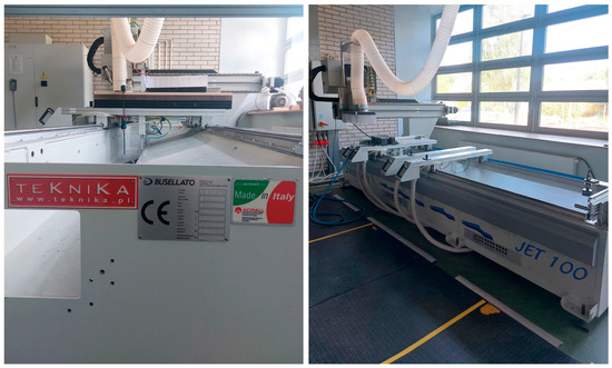
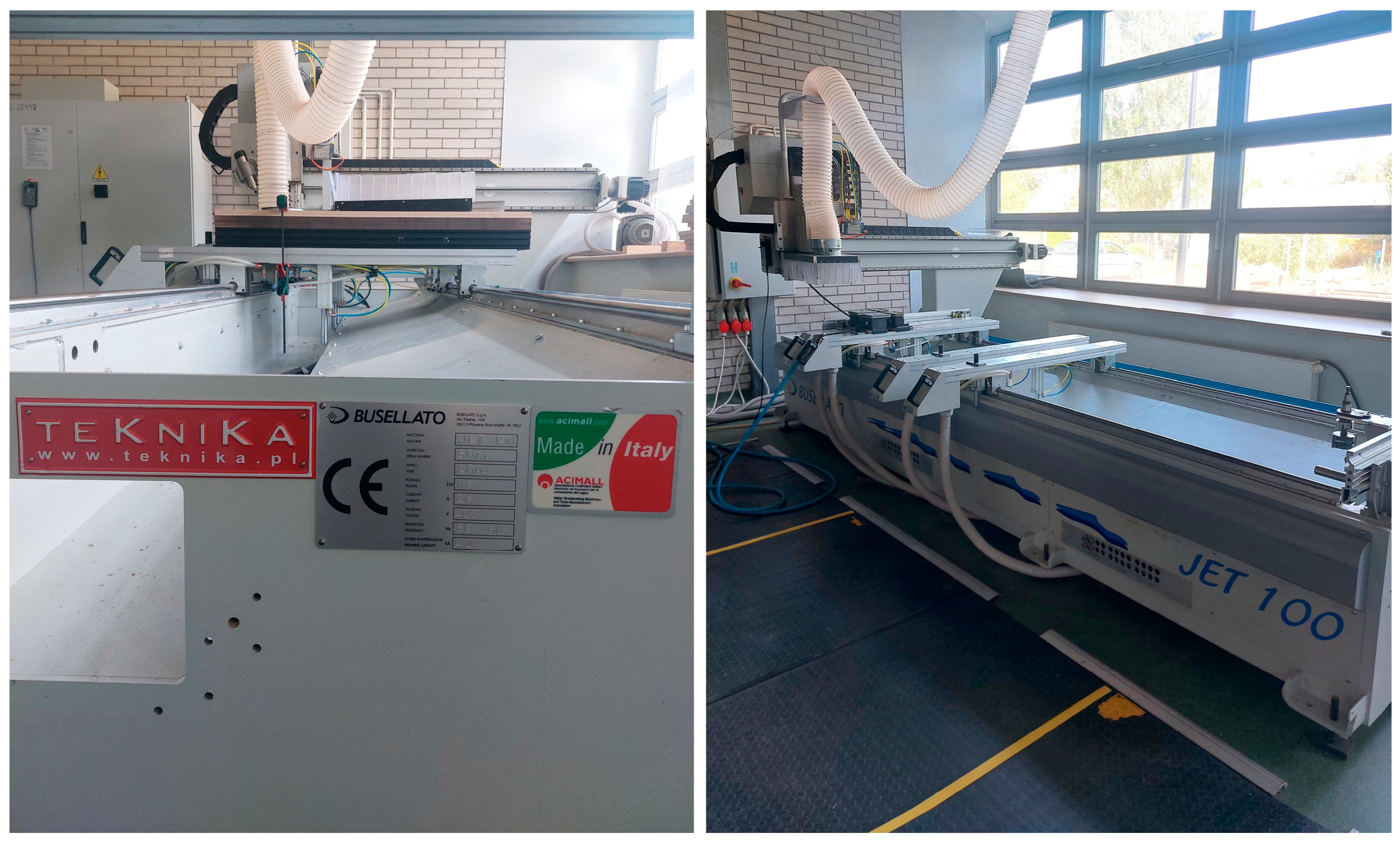
The experiment was conducted on a standard industrial vertical CNC milling center, Busselato Jet 130 (Busellato, Piovene Rocchette, Italy, manufactured in 2004), equipped with TPA Genesis Evolution software, version 3.3 (Figure 1).

Figure 1. The vertical CNC milling center, Busselato Jet 130 used in the study.

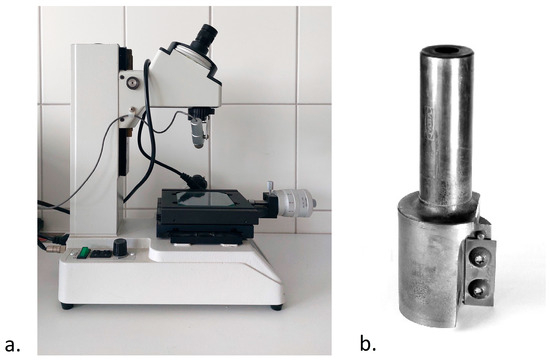
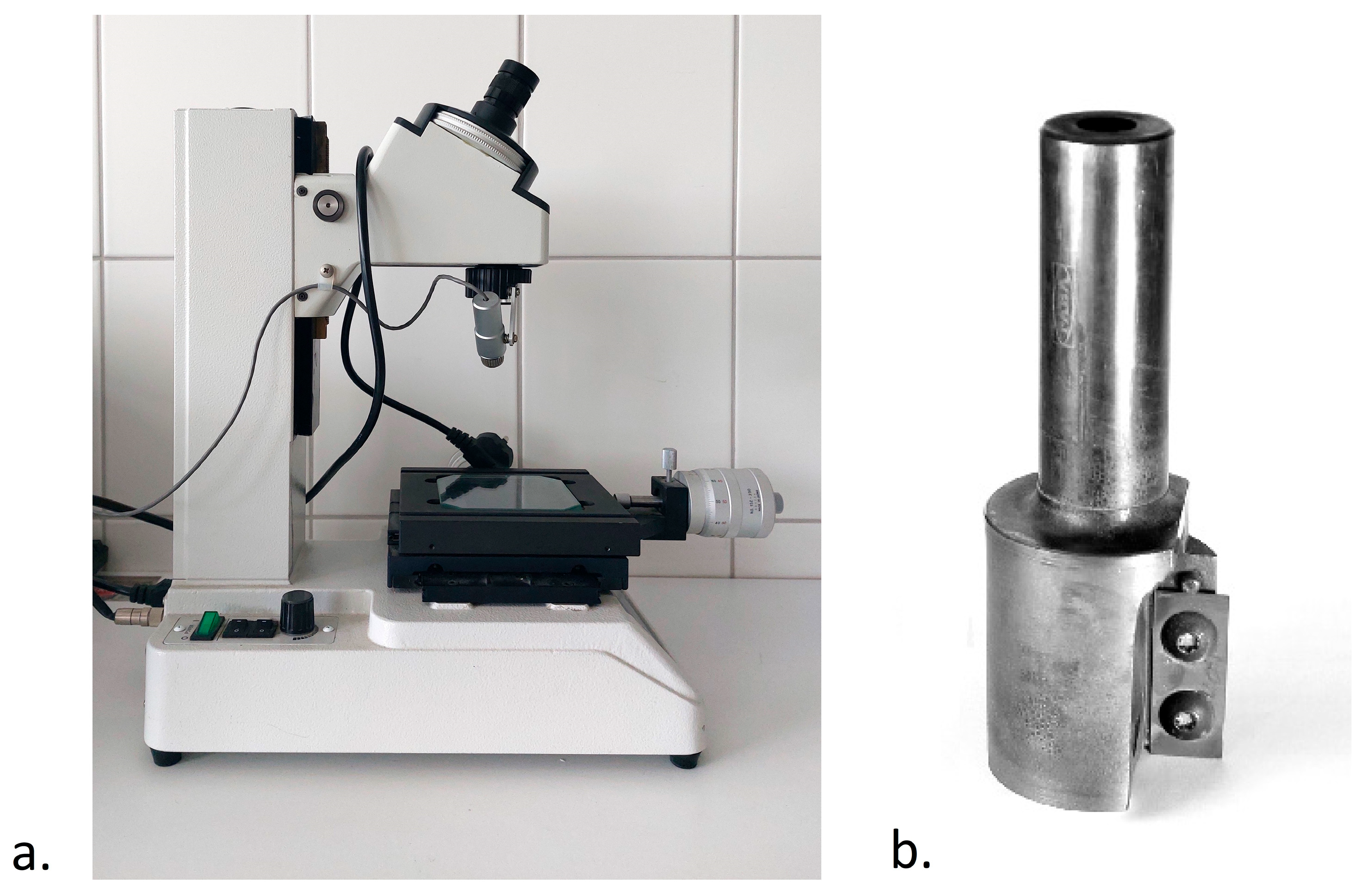
The machine tool was equipped with a milling head (40 mm diameter) featuring replaceable tungsten carbide inserts manufactured by FABA (catalog number: FTS-07). The experiment was conducted with a spindle speed of 18,000 RPM and the feed per tooth was 0.15 mm. Tool wear was periodically measured using a standard Mitutoyo TM-505 microscope (Mitutoyo, Kawasaki, Japan, manufactured in 2017), (Figure 2). The flank wear was measured—specifically, the standard wear indicator known as VB.

Figure 2. Mitutoyo TM-505 microscope (a) and 40 mm diameter milling head (b).

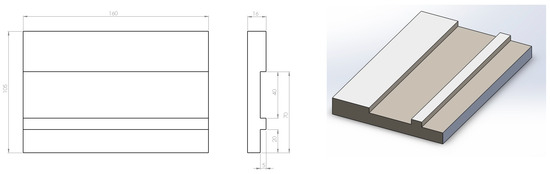
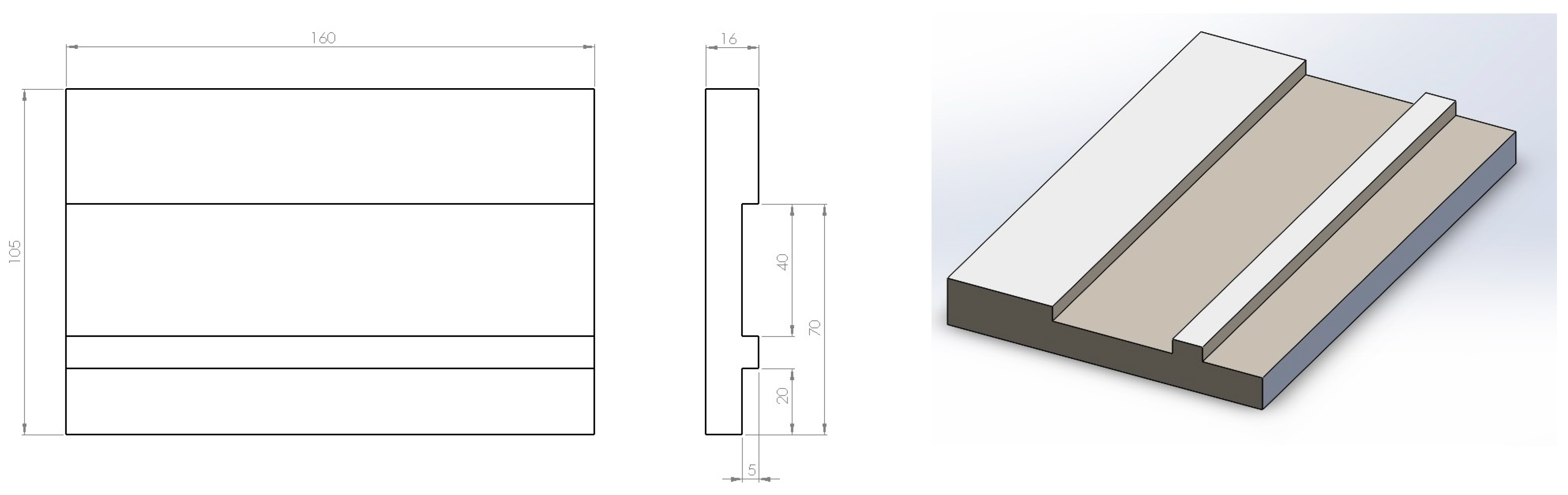
The experiment used white melamine-coated MDF boards from Kronospan (catalog number: K110 SM). The MDF boards measured 2800 × 2070 mm with a thickness of 16 mm. These boards were cut into workpieces with dimensions of 160 mm × 105 mm × 16 mm. Each piece had a groove milled with a depth of 5 mm and a width of 40 mm, as well as single-sided face milling, performed with a depth of 5 mm and a width of 20 mm (Figure 3).

Figure 3. Shape and dimensions of the machined workpieces.

The study used 10 replaceable blades that gradually became increasingly worn. The workpieces (with the shape shown in Figure 3) were produced at various tool wear levels, which were directly monitored using a microscope. For each wear condition, a series of 5 workpieces was produced. Different degrees of wear on individual blades were obtained by milling various wood-based materials, reflecting typical milling tool usage under real industrial conditions.

2.2. Dataset Description and Organization

The dataset consisted of scanned images of machined melamine-faced MDF workpieces produced under different tool wear conditions. Tool wear was quantified using the flank wear indicator VB and grouped into four wear classes (Table 1):

Table 1. Dataset composition.

Wear Class	VB Range (mm)	Number of Workpieces
Class I	0–0.1	90
Class II	0.1–0.2	120
Class III	0.2–0.3	95
Class IV	0.3–0.4	140
Total	–	445

• Class I: VB = 0–0.1 mm;
• Class II: VB = 0.1–0.2 mm;
• Class III: VB = 0.2–0.3 mm;
• Class IV: VB = 0.3–0.4 mm.

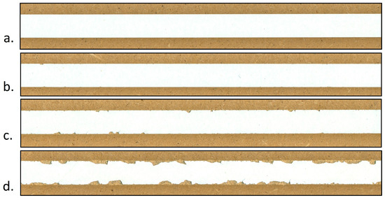
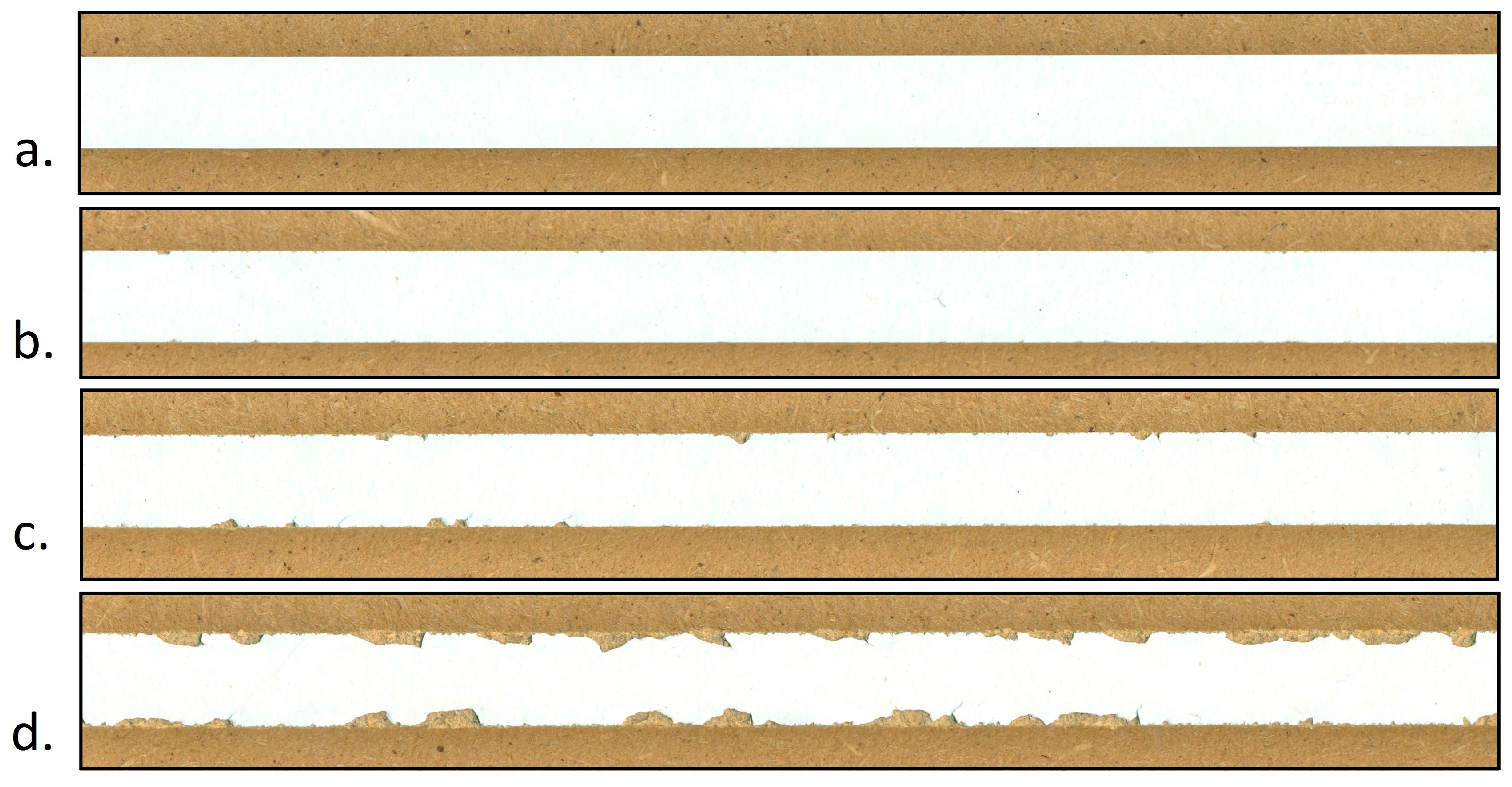
A total of 445 workpieces were collected during the experiment, including 90 samples in Class I, 120 samples in Class II, 95 samples in Class III, and 140 samples in Class IV. Example images representing different classes are shown in Figure 4.

Figure 4. Example images representing different classes: (a) Class I (VB = 0–0.1 mm); (b) Class II (VB = 0.1–0.2 mm); (c) Class III (VB = 0.2–0.3 mm); (d) Class IV (VB = 0.3–0.4 mm).

Each workpiece contained three machined edges that were analyzed independently. Consequently, the image dataset was organized into twelve directories where K1–K4 denote tool wear classes and A–C denote the three machined edges of each workpiece (Table 2):

Table 2. Division into twelve directories.

Wear Class	Edge A	Edge B	Edge C
Class I	K1_A	K1_B	K1_C
Class II	K2_A	K2_B	K2_C
Class III	K3_A	K3_B	K3_C
Class IV	K4_A	K4_B	K4_C

All workpieces were scanned using a SAMSUNG Xpress M2875ND scanner at a resolution of 600 dpi. Owing to the standardized scanning procedure, regions of interest could be extracted automatically using fixed coordinates. For each edge image, a region measuring 250 × 3900 pixels was extracted and rotated so that the laminated surface was always located at the bottom of the image.

To increase the number of training samples and capture local manifestations of edge damage, each edge image was divided into 28 overlapping image windows of size 250 × 250 pixels. The first 100 pixels were omitted, and subsequent windows were extracted every 125 pixels, resulting in a 50% overlap between neighboring windows (Table 3):

Table 3. Image-generation procedure.

Parameter	Value
Scanner resolution	600 dpi
Edge image size	250 × 3900 px
Window size	250 × 250 px
Number of windows per edge	28
Number of edges per workpiece	3
Number of windows per workpiece	84
Window overlap	50%
Total number of image windows	>37,000

Dataset partitioning was performed at the workpiece level rather than at the image-window level. Therefore, all image windows originating from the same workpiece and its corresponding A, B, and C edge images were assigned to the same subset. This procedure eliminated information leakage between training, validation, and testing datasets.

2.3. Model Performance Evaluation

Classification performance was evaluated at three hierarchical levels:

• Image-window level—individual 250 × 250 pixel windows.
• Edge level—complete machined edges represented by 28 image windows.
• Workpiece level—complete workpieces represented by three machined edges (84 image windows).

Two aggregation strategies were investigated.

Over-50% Criterion

A class label was assigned to an edge or workpiece only if more than 50% of all image windows were classified as the same class. If the correct class exceeded the 50% threshold, the prediction was considered correct. If another class exceeded the threshold, the prediction was considered incorrect. If no class exceeded the threshold, the object was classified as unrecognized.

Dominating-Class Criterion

The predicted class corresponded to the most frequently occurring class among all image-window predictions. If the correct class received the largest number of votes, the prediction was considered correct. If an incorrect class received the largest number of votes, the prediction was considered incorrect. If two or more classes obtained the same highest number of votes, the object was considered unrecognized.

For each evaluation level, the number and percentage of correctly classified image windows, edges, and complete workpieces were recorded.

2.4. Data Preparation

All image-processing and deep-learning procedures were implemented in Python 3.11 using the PyTorch 2.7 framework and associated scientific-computing libraries. Image preprocessing was implemented using the torchvision.transforms package and consisted of three operations:

• Resizing each image to 224 × 224 pixels;
• Conversion of image data into PyTorch tensor format;
• Normalization using ImageNet statistics.

The normalization parameters were:

• Mean = [0.485, 0.456, 0.406];
• Standard deviation = [0.229, 0.224, 0.225].

These normalization parameters correspond to the standard preprocessing procedure commonly used for Vision Transformer architectures and improve optimization stability during training. No handcrafted features or manually engineered descriptors were used. The classifier operated directly on normalized RGB image data.

2.5. Research Methodology and Model Architecture

Image classification was performed using the EVA-02 Vision Transformer architecture. The model was adapted for a four-class classification problem corresponding to the four predefined tool wear categories. The final classification layer was replaced with a four-neuron output layer. The model was implemented using publicly available Python libraries supporting EVA-02 architectures. Unless otherwise specified, all architectural and implementation parameters followed the default settings provided by the corresponding libraries. The network was trained from scratch using randomly initialized weights (pretrained = False). The optimization objective was the CrossEntropyLoss function. Optimization was performed using the AdamW optimizer with a learning rate of 3 × 10⁻⁴ and weight decay equal to 0.0. The learning rate was dynamically controlled using the OneCycleLR scheduler. During training, the learning rate increased from an initial value of 5 × 10⁻⁵ to a maximum value of 3 × 10⁻⁴ and subsequently decreased below the initial value. The maximum number of training epochs was set to 200 (Table 4). The best-performing model was selected according to validation-set performance and early stopping was applied to reduce overfitting.

Table 4. Training configuration.

Parameter	Value
Architecture	EVA-02
Number of classes	4
Input image size	224 × 224 px
Weight initialization	Random (pretrained = False)
Loss function	CrossEntropyLoss
Optimizer	AdamW
Learning rate	3 × 10−4
Weight decay	0.0
Learning-rate scheduler	OneCycleLR
Maximum number of epochs	200
Early stopping	Validation-loss based

To obtain statistically robust performance estimates, repeated hold-out validation was employed. For each experiment, 50% of the workpieces were randomly assigned to the training set, 10% to the validation set, and 40% to the testing set (Table 5). Ten independent dataset partitions were generated using different random seeds. For each partition, the training procedure was repeated five times using different model-initialization seeds.

Table 5. Validation protocol.

Parameter	Value
Training set	50%
Validation set	10%
Testing set	40%
Independent dataset partitions	10
Training repetitions per partition	5
Total training runs	50
Partitioning level	Workpiece level

The directory structure used during the experiments followed the convention:

dataset_split_<partition_id>50_10_40

where partition_id denotes the dataset partition identifier and seed denotes the random initialization seed.

Each training run generated an evaluation file according to the convention:

evaluation_results_best_eva02_model__<validation_score>.csv.

The final results reported in this study were obtained from 50 independent training runs. Reported performance values correspond to averages across all runs, thereby reducing the influence of a particular random split or model initialization and providing a more reliable estimate of classifier generalization performance.

2.6. Rules for Establishing Classification Metrics

The efficiency of automatic tool condition monitoring was tested using various approaches to identify the optimal one. For the best-performing approach, formal classification metrics were established. Specifically, three standard metrics—“Precision”, “Recall” and “F1-score”—were calculated for each of the four tool wear states. Additionally, the “Overall Classification Accuracy” was determined.

“Precision” quantifies the reliability of positive predictions made by a model. It determines the proportion of instances flagged as positive that are genuinely correct, thereby indicating the model’s resistance to triggering false alarms.

“Recall” evaluates a model’s capacity to detect all relevant instances within a dataset. It measures the percentage of actual positive cases that the system successfully identifies, reflecting how thoroughly the model captures the target class without overlooking critical data.

“F1-score” serves as a balanced performance indicator by calculating the harmonic mean of precision and recall. It delivers a unified metric that becomes particularly essential when dealing with uneven class distributions, ensuring that a model does not achieve high accuracy at the cost of missing critical errors.

“Overall classification accuracy” represents the comprehensive success rate of a predictive model. It quantifies the proportion of all test instances—across every single category—that the system assigned to their correct classes out of the total number of evaluations made.

A detailed discussion of these concepts and the principles for their calculation are widely known and readily accessible [34].

3. Results

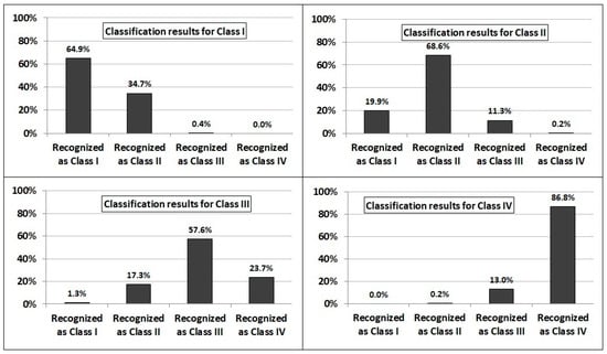
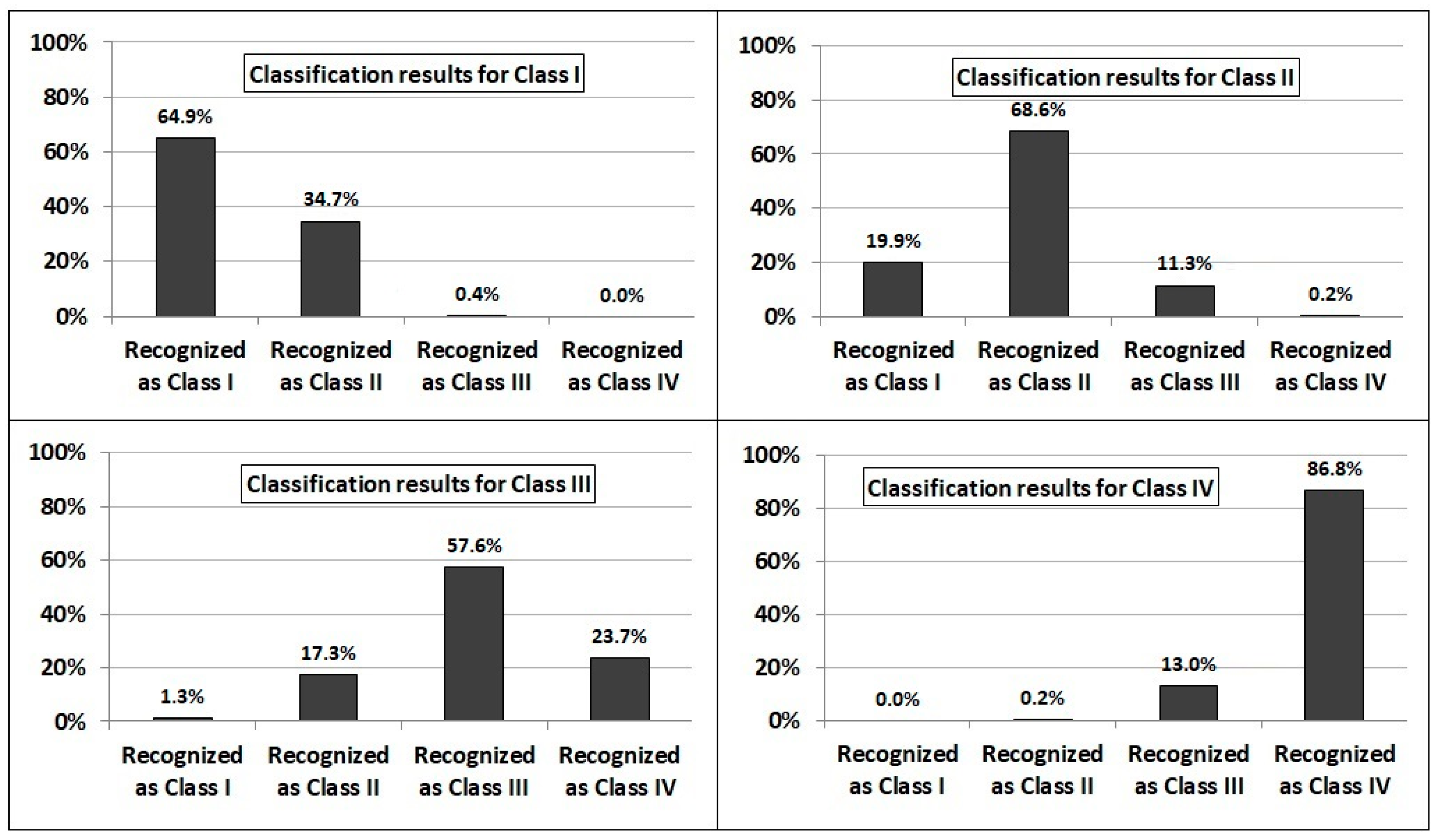
Figure 5 shows the results of the classification of individual sub-images (as a reminder—28 such sub-images were analyzed along each edge of the machined object). The accuracy of the classification largely depended on the true class of the object. The most easily recognized was Class IV (VB = 0.3–0.4 mm), with over 86% of the objects correctly identified. The least effective classification was for Class III (VB = 0.2–0.3 mm), where only 57% of the objects were correctly identified. For the remaining two classes, the classification accuracy was approximately 65%.

Figure 5. Classification results of all single sub-images.

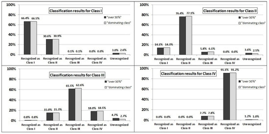
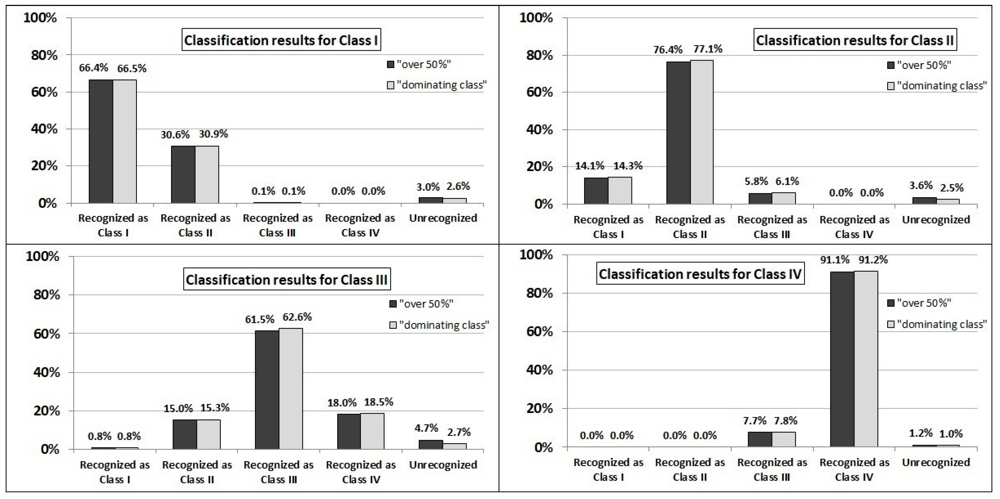
A noticeable, though not drastic, improvement in classification accuracy (by a few percentage points) was achieved when the wear condition was classified not based on a single sub-image, but on a set of 28 sub-images located along the same edge (Figure 6). As a result, the recognition rate for Class IV slightly exceeded 90%, and the recognition rate for Class III also improved somewhat, slightly surpassing 60%. Both tested criteria (“over 50%” and “dominating class”) yielded comparable results, although the latter appeared to be slightly more effective (the differences generally did not exceed 1%).

Figure 6. Classification results of individual edges (28 sub-images were analyzed for each edge) according to the “over 50%” and the “dominating class” criteria.

In addition, only a very small percentage of cases involved images for which it was not possible to determine the dominant class, i.e., the object could not be recognized. These values ranged from 1% to 2.7%. For the “over 50%” criterion, the percentage of unrecognized objects was slightly higher, ranging from 1.2% to 4.7%.

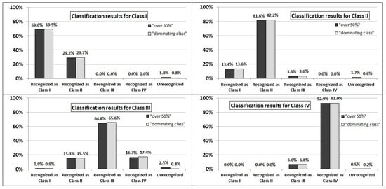
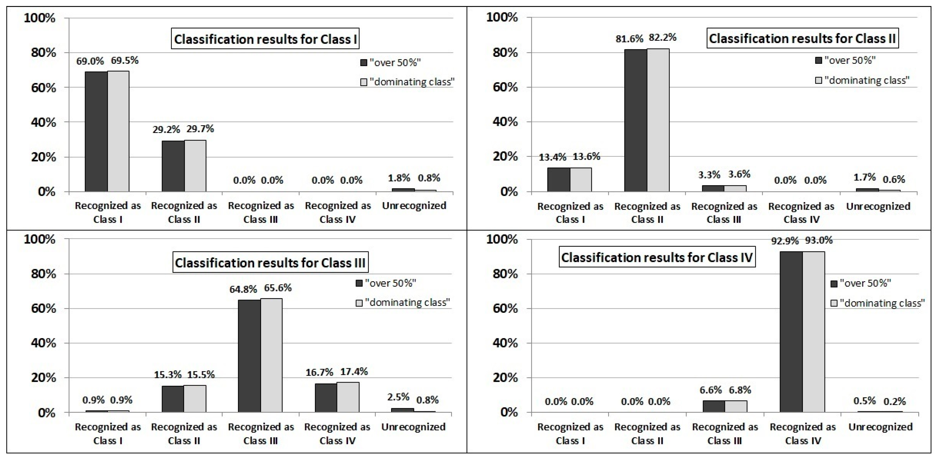
As expected, the best classification results were obtained when the tool wear condition was assessed based on the analysis of all three edges of the same machined object (i.e., based on the analysis of 3 × 28 sub-images). The results of this classification are shown in Figure 7. The highest recognition rate (93%) was achieved for Class IV, followed by Class II (77%). The least recognizable was Class III, with a recognition rate of 65%.

Figure 7. Classification results of entire workpieces (for each workpiece a set of 3 edges were analyzed, i.e., 3 × 28 sub-images) according to the “over 50%” and the “dominating class” criteria.

As in the previous case, both tested criteria (“over 50%” and “dominating class”) yielded comparable results. Again, the latter appeared to be slightly more effective, although the differences did not exceed 1%. The percentage of unrecognized objects for the “dominating class” criterion ranged from 0.2% to 0.8%, while for the “over 50%” criterion, it ranged from 0.5% to 2.5%.

As described in Section 2.6, the formal classification metrics (Precision, Recall, and F1-score) were calculated for each of the four tool wear states using the best-performing variant. This optimal variant involved the classification of entire workpieces based on the “dominating class” criterion, where a set of three edges (comprising 3 × 28 sub-images) was analyzed for each workpiece. The results of these calculations are presented in Table 6. Additionally, the Overall Classification Accuracy was determined for this variant of classification. This accuracy was 79%.

Table 6. Classification metrics for evaluating entire workpieces based on the “dominating class” criterion (the data presented in the table was calculated taking into account the varying sample sizes of each class and was based on the results shown in Figure 7).

Wear Class	Precision	Recall	F1-Score
Class I	78.5%	69.5%	73.7%
Class II	70.4%	82.2%	75.8%
Class III	81.8%	65.5%	72.7%
Class IV	88.7%	93.0%	90.8%

4. Discussion

In summary, it can be stated that the general classification accuracy achieved in the most favorable scenario (classification based on the photographic image of the entire sample, using the “dominating class” criterion) was approximately 79%. This result is promising, though certainly not entirely satisfactory. When attempting to compare this outcome with the results of earlier research projects of a similar nature, it is important to emphasize that virtually all of them were conducted in Poland. This is by no means the result of a biased selection of scholarly publications. Rather, it stems from the fact that Polish researchers predominantly specialize in this specific line of inquiry. This trend is likely closely correlated with the pivotal importance of the Polish furniture industry to the country’s overall economy. As Europe’s top furniture exporter and third-largest manufacturer in UE, Poland ranks third globally in foreign sales and seventh in overall production [35]. Moreover, it should be emphasized that all these previous studies involved drilling rather than milling, and that they involved three-class classification, rather than four-class classification. Nevertheless, comparing their overall classification accuracies is meaningful and has been presented in Table 7. The classification accuracies obtained in earlier studies range from 67% to 82%. Therefore, it can be said that the use of the EVA-02 model yields similarly promising results (79%); however, from a practical standpoint, these outcomes are generally not fully satisfactory. Regrettably, due to the aforementioned methodological differences (milling versus drilling and a four-class versus three-class classification system), a profound and more comprehensive comparison or discussion of these research results is difficult to conduct. For instance, it is highly probable that if a three-class classification system had been adopted, following the approach of previous studies, the classification accuracy rates would have been slightly higher. Nonetheless, a comparison of the overall classification accuracy presented in Table 7 appears entirely justified and supports the conclusion that the application of EVA-02 classifier did not yield a spectacular breakthrough. It is crucial to document this limited performance as clearly as possible to avoid any misconceptions to the contrary. In any case, further research in this field remains essential, and Polish furniture factories must still await the commercial availability of tool condition monitoring systems.

Table 7. Comparison of overall classification accuracy achieved in various research projects on automatic monitoring of the condition of tools used for machining wood-based materials.

Research Project	Type of Analyzed Data	Classification Strategy (Algorithm)	The Best General Classification Accuracy
The study presented in this article	Digital images of workpieces	EVA-02 model	79%
Jegorowa, A., Górski, J., Kurek, J., Kruk M. (2019) [13]	Digitalized signals of cutting forces, noise, acoustic emission, and acceleration of jig vibrations	Support vector Machine (SVM)	81%
Jegorowa, A., Antoniuk, I., Kurek, J., Bukowski, M., Wioleta, D., Czarniak, P. (2020) [17]	Digital images of workpieces	Convolutional neural networks (CNN)	77%
Jegorowa, A., Górski, J., Kurek, J., Kruk, M. (2020) [14]	Digitalized signals of cutting forces, noise, acoustic emission, and acceleration of jig vibrations	K-nearest neighbors (k-NN)	76%
Kurek, J., Krupa, A., Antoniuk, I., Akhmet, A., Abdiomar, U., Bukowski, M., Szymanowski, K. (2024) [21]	Digital images of workpieces	Siamese Networks	82%
Jegorowa, A., Kurek, J., Antoniuk, I., Dołowa, W., Bukowski, M., Czarniak, P. (2021) [18]	Digital images of workpieces	Deep learning	80%
Bukowski, M., Kurek, J., Antoniuk, I., Jegorowa, A. (2021) [22]	Digital images of workpieces	Light gradient boosting machine (LGBM)	67%

5. Conclusions

The publication presents the results of a study using a classifier based on the EVA-02 model to identify tool wear during the milling of laminated MDF boards. The most accurately recognized tool wear class was Class IV (Precision 89%; Recall 93% and F1-score 91%—rounded to whole numbers). However, the classification metrics for the remaining classes were considerably lower. For instance, the F1-score for each of them fell well below 80%. Most notably, the recall for class III was particularly poor, reaching a mere 65%.

Overall, the classification performance for all classes except Class IV seems inadequate for practical applications. Considering all primary classification metrics—particularly the F1-score, which typically holds the greatest practical significance in engineering projects—it can be concluded that the discriminability of Class III does not differ significantly from that of Class II or Class I. The superior discriminability of Class IV appears to stem from the fact that tools with extreme wear (VB > 0.3 mm) induce highly distinct damage to the workpiece edge in the form of delamination (Figure 4d).

The overall accuracy, averaged across all four classes, was 79%. This result is comparable to previous research reports and can be considered promising. However, the problem of Tool Condition Monitoring (TCM) in the furniture industry still requires further research to develop a classifier with even higher effectiveness.

For future research, it is worth returning to a three-class tool condition monitoring approach, which is sufficient from a practical standpoint. Additionally, integrating the blade condition monitoring system with machining quality evaluation remains a promising direction. However, this will require a broader scope of experimental testing utilizing more advanced computer vision and artificial intelligence algorithms.

References

- Bedelean, B.; Ispas, M.; Răcăsan, S. Optimizing Wood Composite Drilling with Artificial Neural Network and Response Surface Methodology. Forests 2024, 15, 1600. [Google Scholar] [CrossRef] [Scilit]
- Teti, R.; Jemielniak, K.; O’Donnell, G.; Dornfeld, D. Advanced monitoring of machining operations. CIRP Ann. 2010, 59, 717–739. [Google Scholar] [CrossRef] [Scilit]
- Wang, Q.; Wang, H.; Hou, L.; Yi, S. Overview of Tool Wear Monitoring Methods Based on Convolutional Neural Network. Appl. Sci. 2021, 11, 12041. [Google Scholar] [CrossRef] [Scilit]
- Śmietańska, K.; Podziewski, P.; Bator, M.; Górski, J. Automated monitoring of delamination factor during up (conventional) and down (climb) milling of melamine-faced MDF using image processing methods. Eur. J. Wood Wood Prod. 2020, 78, 613–615. [Google Scholar] [CrossRef] [Scilit]
- Szwajka, K.; Trzepieciński, T. The influence of machining parameters and tool wear on the delamination process during milling of melamine-faced chipboard. Drewno 2017, 60, 118–131. [Google Scholar] [CrossRef] [Scilit]
- Trzepieciński, T.; Szwajka, K.; Zielińska-Szwajka, J.; Szewczyk, M. Current Trends in Monitoring and Analysis of Tool Wear and Delamination in Wood-Based Panels Drilling. Machines 2025, 13, 249. [Google Scholar] [CrossRef] [Scilit]
- Zhu, Q.; Sun, W.; Zhoua, Y.; Gao, C. A tool wear condition monitoring approach for end milling based on numerical simulation. Maint. Reliab. 2021, 23, 371–380. [Google Scholar] [CrossRef] [Scilit]
- Zhou, Y.; Liu, C.; Yu, X.; Liu, B.; Quan, Y. Tool wear mechanism, monitoring and remaining useful life (RUL) technology based on big data: A review. SN Appl. Sci. 2022, 4, 232. [Google Scholar] [CrossRef] [Scilit]
- Turšic, N.; Klancnik, S. Tool Condition Monitoring Using Machine Tool Spindle Current and Long Short-Term Memory Neural Network Model Analysis. Sensors 2024, 24, 2490. [Google Scholar] [CrossRef] [Scilit] [PubMed]
- Rehman, A.; Salwa Rabbi Nishat, T.; Uddin Ahmed, M.; Begum, S.; Ranjan, A. Chip Analysis for Tool Wear Monitoring in Machining: A Deep Learning Approach. IEEE Access 2024, 12, 112672–112689. [Google Scholar] [CrossRef] [Scilit]
- Serin, G.B.; Sener, A.M.; Ozbayoglu, H.O. Review of tool condition monitoring in machining and opportunities for deep learning. Int. J. Adv. Manuf. Technol. 2020, 109, 953–974. [Google Scholar] [CrossRef] [Scilit]
- Mohamed, A.; Hassan, M.; M’Saoubi, R.; Attia, H. Tool Condition Monitoring for High-Performance Machining Systems—A Review. Sensors 2022, 22, 2206. [Google Scholar] [CrossRef] [Scilit] [PubMed]
- Jegorowa, A.; Górski, J.; Kurek, J.; Kruk, M. Initial study on the use of support vector machine (SVM) in tool condition monitoring in chipboard drilling. Eur. J. Wood Wood Prod. 2019, 77, 957–959. [Google Scholar] [CrossRef] [Scilit]
- Jegorowa, A.; Górski, J.; Kurek, J.; Kruk, M. Use of nearest neighbors (k-NN) algorithm in tool condition identification in the case of drilling in melamine faced particleboard. Maderas-Cienc. Tecnol. 2020, 22, 189–196. [Google Scholar] [CrossRef] [Scilit]
- Dong, W.; Xiong, X.; Ma, Y.; Yue, X. Woodworking Tool Wear Condition Monitoring during Milling Based on Power Signals and a Particle Swarm Optimization-Back Propagation Neural Network. Appl. Sci. 2021, 11, 9026. [Google Scholar] [CrossRef] [Scilit]
- Szwajka, K. Laboratory versus industrial cutting force sensor in tool condition monitoring system. J. Phys. Conf. Ser. 2005, 13, 377–380. [Google Scholar] [CrossRef] [Scilit]