Transfer-Function Modeling and Modal Characterization of Wooden Beam Specimens Based on Frequency Response Functions

Abstract

This study utilized three controlled Sitika spruce beam specimens and established a parameterized transfer-function model based on force–acceleration frequency response functions (FRFs) to characterize and reconstruct the frequency-domain modal response of beam specimens. The specimens were tested using non-contact magnetic swept-sine excitation, laser Doppler vibration measurement, and synchronous FFT analysis methods under free–free boundary conditions. In the experiment, one specimen was used for modeling and the other two specimens were used for consistency verification. Based on the measured complex FRF, a 1st–5th order modal transfer-function model was established in the frequency range of 0–1000 Hz. The experiment identified five resonance frequencies of the specimen, which were 65.0, 198.5, 370.5, 620.0, and 930.0 Hz, respectively. The model can reconstruct the measured magnitude and phase responses, with magnitude residuals within ±5 dB, resonance-peak magnitude errors of 0.03–0.73 dB, and wrapped-phase deviation around the poles of 0.20–5.08°. The Nyquist trajectory was continuous and smooth, with all poles located in the left half-plane, indicating that the model has stable pole behavior. The research results support the specimen vibration response as an approximate linear time-invariant system under small-magnitude and controlled testing conditions. The model can provide a physically interpretable and reconstructable modal-parameter expression for evaluating frequency-domain vibration responses of controlled wooden beam specimens.

1. Introduction

Wood is widely used in musical instruments; load-bearing timber structural components, such as beams, columns, and glued-laminated members; and wood-based composite panels. Its vibration behavior is controlled by the hierarchical and anisotropic structure of wood, including cell arrangement and differentiation; anatomical differences in the longitudinal, radial, and tangential directions; cell wall microfibril angle; chemical composition; early–latewood distribution, juvenile–mature wood variation; and moisture content. These factors can affect the stiffness, density distribution, and energy dissipation behavior of wood, resulting in direction dependence of modal frequencies, damping characteristics, and frequency response. In multi-degree-of-freedom systems such as plates and beams, energy can be coupled and redistributed between different modes. In this case, it is often difficult to trace the path of energy transfer only from time-domain responses. Therefore, establishing a transfer function between input and output in the frequency domain and analyzing its dynamic mechanism can provide an effective method for understanding the vibration behavior of wood [1,2,3,4,5,6].

The transfer function can describe the magnitude and phase characteristics of the input–output relationship in a unified frequency domain and also provides a basis for identifying modal parameters such as natural frequency, damping ratio, and mode shape. These parameters not only quantify the contribution of each mode to the overall response, but also provide important references for structural dynamic analysis, modal identification, finite element model updates, and the dynamic performance evaluation of wood components. Previous studies have shown that modal analysis and frequency-domain identification methods can characterize dynamics of wood and wood-based structural elements. However, the identification accuracy is still affected by testing conditions, signal-to-noise ratio, and post-processing methods. Therefore, establishing a stable and reproducible transfer-function model for wooden beam specimens has clear methodological significance for frequency-domain feature identification, parameter reliability improvement, and response reconstruction of wood dynamics [7,8,9,10,11,12,13,14].

Many previous studies, including those by Zhang et al. [15], Deng et al. [16], Kohantorabi et al. [17], Ahmed and Adamopoulos [18], and Guan et al. [19], have obtained FRF using excitation methods such as blades, impact hammers, and steel balls. These studies usually focus more on low-order resonance frequencies and damping-related indicators, with less research on higher-order modal responses, magnitude–phase relationships, and the conversion of measured FRFs into physically interpretable transfer-function parameters. Due to the difficulty in completely repeating the excitation waveform, excitation point position, and excitation direction, these methods may reduce the repeatability of the identified magnitude and phase responses, affecting the consistency of modal-parameter extraction [20,21]. Merhar et al. [22] used a “small hammer + microphone” method to measure the impact response of spruce beams, and then extracted the damping of the first three modes by combining envelope fitting and wavelet transform, with further analysis of its variation with moisture content. Lämmlein et al. [23] compared the FRFs of spruce plates before and after different coating steps by using a “small hammer + laser Doppler vibrometer (LDV)” approach. They quantitatively evaluated the effects of coating on natural frequencies and damping ratios, and provided experimental FRF data for different coating stages, offering a reference for the acoustic optimization of plates. In studies on the wolf note of bowed string instruments, Inácio et al. [24] established a computational model of string–body coupling based on measured body FRFs. By introducing a linear modal model at the bridge and coupling it with the frictional nonlinearity of the string, the wolf note in the violin family was successfully reproduced numerically. However, most existing models are still based on overall FRFs or simplified structural parameters, and there are still limitations in the conversion of tonewood FRFs into physically interpretable modal parameters at the material component scale. Therefore, this study focuses on Sitka spruce, a typical tonewood, and develops a reproducible transfer-function identification method for modal characterization at the material component scale, providing a parameterized basis for evaluating and reconstructing the frequency-domain vibration responses of wooden beam specimens, and also providing information for the future model development of wooden soundboard materials [25,26].

This study aims to establish a physically interpretable transfer-function framework based on measured force–acceleration frequency response functions for the modal characterization of Sitka spruce beam specimens. The study transforms the experimentally measured FRFs from discrete resonance-peak to pole–residue expressions, in order to describe resonance frequencies, damping ratios, modal residues, magnitude–phase evolution, and complex-plane response characteristics. The experiment utilized Sitka spruce beam specimens and tested them in the frequency range of 50–1000 Hz under small-magnitude vibration and controlled-moisture-content conditions using non-contact magnetic swept-sine excitation, dual-channel laser Doppler vibrometry, and FFT analysis methods. Based on modal superposition, an analytical transfer-function model was established, and the model was validated through Bode magnitude–phase plots, Nyquist plots, and time-domain reconstruction. A set of modal parameters, $\left\{{\omega }_r,{\zeta }_r,R_r\right\}$, was extracted for a low-dimensional parameterization description of the dominant dynamic responses of the wooden beam specimens. Among them, $r$ is the modal order, ${\omega }_r$ is the natural angular frequency, ${\zeta }_r$ is the modal damping ratio, and $R_r$ is the modal residue. The studied model can provide a parameterized basis for evaluating the vibration characteristics of wooden beam specimens and interpreting the coupling relationship between excitation and response modes.

2. Materials and Methods

2.1. Materials and Instrumentation

2.1.1. Test Materials

According to Euler–Bernoulli beam theory, when the ratio of length $L$ to thickness $h$ of a specimen satisfies $L/h>20$, the effects of shear deformation and rotary inertia are generally small for low-order bending vibration. When the ratio of length $L$ to width $b$ satisfies $L/b>15$, the specimen can be approximately regarded as a one-dimensional beam. These geometric criteria were used to support the slender-beam approximation for the present specimens, but they do not imply that shear deformation and rotary inertia are negligible for all higher-order modes. According to ASTM E1876 standard [27], when $4\le b/h\le 10$, the cross-section of the specimen is thin enough to maintain a reasonable distribution of shear stress, while also avoiding excessive warping caused by a flat section. Therefore, the study selected three beam specimens with dimensions of 500 mm × 25 mm × 3 mm.

The specimens were prepared from AA-grade radial Sitka spruce boards (Picea sitchensis (Bong.) Carr.) without visible defects such as cracks, deformation, decay, or discoloration. All surfaces were planned smoothly before testing. The properties of the three specimens were as follows: the latewood percentage of specimens (a), (b), and (c) was 24.59%, 23.86%, amd 23.37%; the moisture content was 6%, 4%, and 6%; and the density was 419.78 kg·m⁻³, 410.11 kg·m⁻³, and 417.23 kg·m⁻³. Specimen (a) was used for model construction, while specimens (b) and (c) were used to verify the consistency and reusability of the modeled process. The three specimens had the same size and moisture contents. The specimens were tested under the same testing conditions, which helped reduce the influence of material and anatomical differences on the validation of the modeling process.

2.1.2. Experimental Equipment and Setup

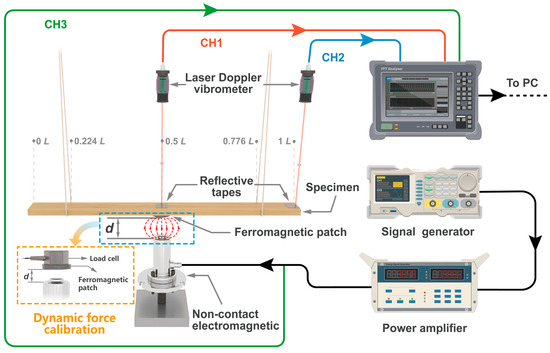
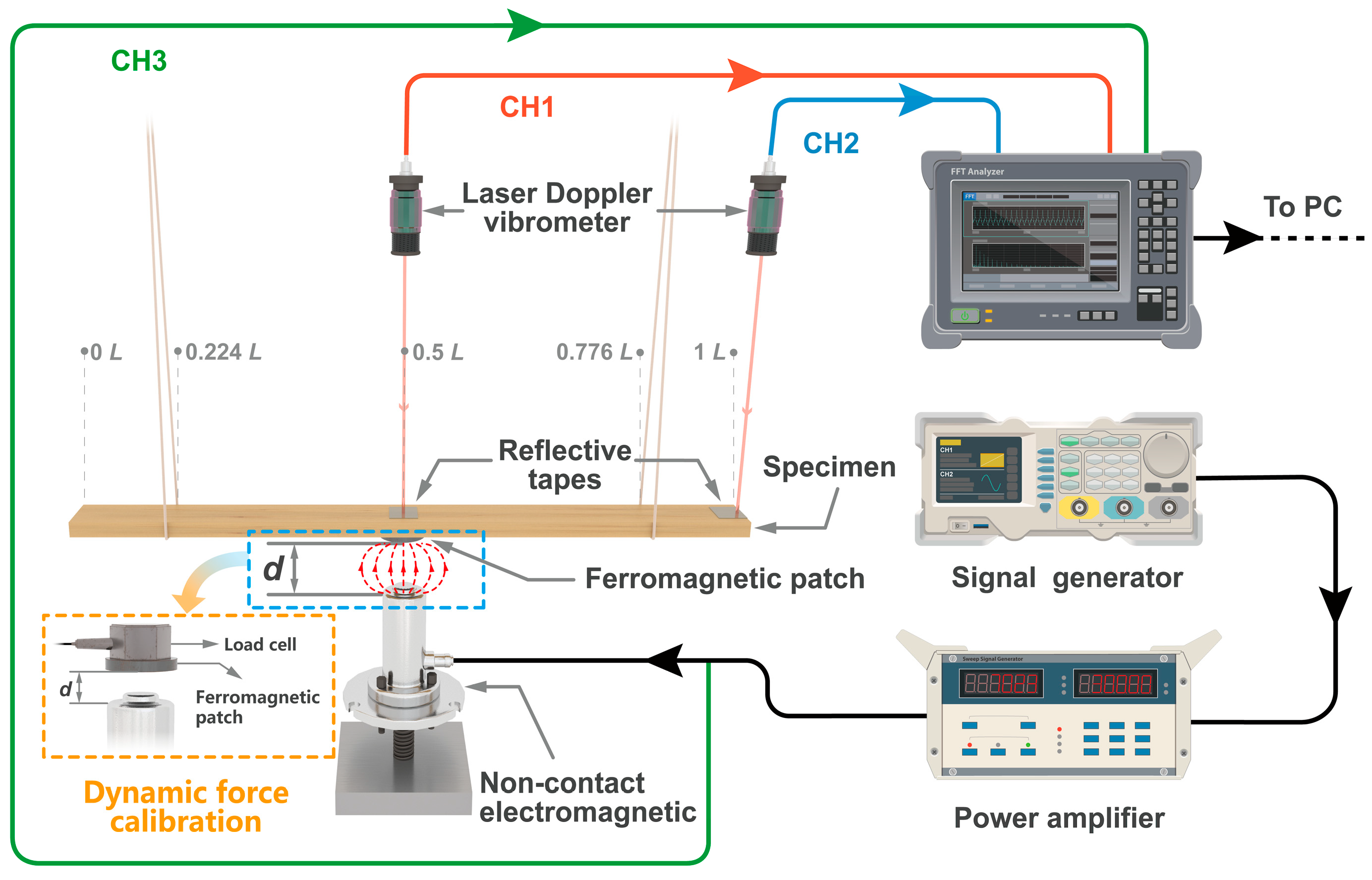
The experimental instruments used included a four-channel FFT analyzer (CF-9400, Ono Sokki, Yokohama, Japan), signal generator (DG1022Z, RIGOL, Suzhou, China), power amplifier (DH1301, Donghua Testing, Taizhou, China), non-contact magnetic exciter (DH41020, Donghua Testing, Taizhou, China), laser Doppler vibrometer (FNV-RD-AVD1, Junda Gaoke, Hefei, China), and IEPE piezoelectric force sensor (KT-YD-3200L, Ketu Electronic, Yangzhou, China). The test setup is shown in Figure 1.

Figure 1. Experimental setup.

2.2. Experimental Procedure

The specimen adopts double-free boundary conditions, and is suspended by a 0.15 mm diameter ultra-high-molecular-weight polyethylene (UHMWPE) fine rope at 0.224 L and 0.776 L (L is set as shown in Figure 1) of the first-order modal node position to minimize the influence of boundary interference on the vibration response. The signal generator outputs a swept-sine excitation signal with a frequency range of 50–1000 Hz, a peak-to-peak value of 10 V, and an initial phase of 0°. The power amplifier operated in constant voltage mode.

To avoid possible effects of nonlinearity, hysteresis, or path dependence, a comparison was made between upward and downward frequency sweeps in the experiment. There were no substantial differences in main resonance frequencies, peak magnitudes, and the overall trend of the FRF curves obtained under the two frequency-sweeping methods. Under the input used for the upward sweep, no observable strong nonlinear behavior was detected. Therefore, the upward-sweep mode was used for data collection in the experiment.

Due to the limited single-sweep duration of the signal source (≤500 s) and the requirement for a relatively slow sweep speed in the lightly damped mode to meet steady-state conditions, a segmented linear sweep-sine frequency was used in the experiment to meet frequency band coverage and suitable sweep speed control. The segmented breakpoint was set in the low-frequency range, because steady-state conditions were more difficult to stabilize in this region, and the first resonance frequency was expected to be between 50 and 100 Hz. Therefore, the sweep duration was set to 200 s for 50–120 Hz and 500 s for 80–1000 Hz. When the scaling conditions of the two segments (including input magnitude, calibration, gain, window/averaging settings, and measurement range) were consistent, the overlapping band was nearly constant and the magnitude was very small (<0.001 dB), which can be directly concatenated together.

To calibrate the excitation force, the force sensor was fixed to a rigid bracket, and the same magnetic patch in the specimen was attached below it. The gap between the magnetic patch and the electromagnetic exciter was 3 mm, and the monitored exciter voltage was used as an input control variable. Keeping the voltage the same under calibration and specimen testing conditions can maintain consistent excitation, ensuring that the excitation force applied to the specimen is the same as under calibration conditions. The experiment measured the gap fluctuation caused by the displacement response of the specimen near the excitation point (with a set gap of 3 mm). Within the excitation and response range of this experiment, this fluctuation is very small relative to the gap, and it can be considered that it will not change the basic excitation state of the experiment, nor will it affect the identification of the main modal parameters.

In an ideal linear system, the response of a single-frequency sinusoidal excitation is mainly concentrated at the fundamental frequency. If the system has strong nonlinearity characteristics, the response spectrum usually contains more significant low-order harmonic components. This study investigated the spectral line distribution near the fundamental frequency and its low-order harmonics and found that the response was still dominated by the fundamental frequency component, with no obvious harmonic peaks competing with the main response. This indicates that the nonlinearity of the electromagnetic excitation chain was weak, and the system can be approximated as linear and time-invariant within the studied frequency range.

The FFT collected and recorded the frequency-domain magnitude of the excitation force as the force input (CH1). The response signal of the free-end LDV represents the structural output (CH2). The exciter voltage was monitored by FFT (CH3). The FFT data was processing used Hanning window function, with a sampling frequency of 10 kHz and a frequency resolution of 0.5 Hz, to obtain the frequency response functions (FRFs) in the frequency range of 50–1000 Hz. The outputs included magnitude plots, phase plots, Nyquist plots, and coherence plots. Based on the FRF magnitude curves, resonance peaks and anti-resonance points of each mode were identified.

2.3. Transfer-Function Model

The vibration of wood under free–free boundary conditions can be regarded as a multi-degree-of-freedom system [28], and its equation of motion can be written as [20]

$$M\ddot{x}\left(t\right)+C\dot{x}\left(t\right)+Kx\left(t\right)=f\left(t\right)$$

(1)

where $M$, $C$, and $K$ are the mass, damping, and stiffness matrices of the specimen, respectively. $x(t$) is the displacement vector of the degrees of freedom, representing the time-varying displacements of the $n$ degrees of freedom, and $f\left(t\right)$ is the external force vector applied to the system. The transfer function between force and displacement can be written as

$$X_j\left(s\right)={\sum }_{r=1}^N{\varphi }_{jr}·{\displaystyle \frac{{\varphi }_{kr}}{s^2+2{\zeta }_r{\omega }_{r}s+{\omega }_r^2}}F\left(s\right)$$

(2)

where $s$ is the complex Laplace variable; $X_j(s)$ is the displacement response in the Laplace domain at the response degree of freedom $j$; $F\left(s\right)$ is the external force input in the Laplace domain applied at the excitation degree of freedom $k$; $N$ is the number of retained modes; $r$ denotes the modal order; ${\varphi }_{jr}$ and ${\varphi }_{kr}$ are the $r$-th mass-normalized mode-shape components at the response and excitation degrees of freedom, respectively; ${\omega }_r$ is the undamped natural angular frequency of the $r$-th mode; and ${\zeta }_r$ is the corresponding modal damping ratio. ${\varphi }_{jr}{\varphi }_{kr}$ describes the modal coupling between the excitation and response locations, while the denominator $s^2+2{\zeta }_r{\omega }_{r}s+{\omega }_r^2$ describes the second-order dynamic behavior of the $r$-th mode according to the modal superposition theory. The transfer function between force and displacement is as follows [29]:

$$H_{disp}(s)={\displaystyle \frac{X_j(s)}{F(s)}}={\sum }_{r=1}^N{\displaystyle \frac{{\varphi }_{jr}{\varphi }_{kr}}{s^2+2{\zeta }_r{\omega }_{r}s+{\omega }_r^2}}$$

(3)

where $H_{disp}\left(s\right)$ is the displacement-to-force transfer function, namely the receptance, between the excitation degree of freedom $k$ and the response degree of freedom $j$; $R_r^{\left(x\right)}$ is the displacement-domain modal residue of the $r$-th mode; and the superscript $\left(x\right)$ indicates that the residue is associated with displacement response. Under mass-normalized modal coordinates,

$$R_r^{\left(x\right)}={\varphi }_{jr}{\varphi }_{kr}$$

(4)

When the response is acceleration, $A_j(s)=s^2{X}_j(s)$, where $A_j(s)$ is the acceleration response at the response degree of freedom $j$ in the Laplace domain. For zero initial conditions, Equation (3) can be written as

$$H_{acc}(s)={\displaystyle \frac{A\left(s\right)}{F\left(s\right)}}={\sum }_{r=1}^N{\displaystyle \frac{s^2{\varphi }_{jr}{\varphi }_{kr}}{s^2+2{\zeta }_r{\omega }_{r}s+{\omega }_r^2}}$$

(5)

$H_{acc}\left(s\right)$ is the force-to-acceleration transfer function, also referred to as accelerance.

$$R_r^{\left(a\right)}(s)=s^2{R}_r^{\left(x\right)}=s^2{\varphi }_{jr}{\varphi }_{kr}$$

(6)

where $R_r^{\left(a\right)}$ is the acceleration-domain modal residue or effective numerator term of the $r$-th modal component, and the superscript $\left(a\right)$ is the acceleration response. Substituting Equation (6) into Equation (5) gives

$$H_{acc}(s)={\sum }_{r=1}^N{\displaystyle \frac{R_r^{\left(a\right)}}{s^2+2{\zeta }_r{\omega }_{r}s+{\omega }_r^2}}$$

(7)

Equation (7) is the expression of the transfer function between force and acceleration in a multi-degree-of-freedom vibration system [29]. In the experiment, swept-sine excitation was used. For a linear time-invariant system, once the transient response decays, the system can be considered to be in a sinusoidal steady state. Set the Laplace variable to $s=\mathrm{j}\omega$, and the value of the transfer function $H\left(s\right)$ on the imaginary axis, namely $H\left(j\omega \right)$, becomes the frequency response function, as shown in Equation (8). The transfer-function model of this study is based on theoretical modal analysis in the $s$-domain and formally represented as the superposition of second-order modal terms. Although the real part is not included in the equation, the frequency response analysis is equivalent to evaluating the system response along the imaginary axis in the $s$-domain, and therefore still belongs to the broad framework of $s$-domain modeling. This method retains the advantages of frequency-domain analysis, while also obtaining system parameters such as damping and modal coupling from the transfer-function model.

$$H_{acc}(\mathrm{j}\omega )={\displaystyle \frac{A\left(\mathrm{j}\omega \right)}{F\left(\mathrm{j}\omega \right)}}={\sum }_{r=1}^N{\displaystyle \frac{-{\omega }^2{\varphi }_{jr}{\varphi }_{kr}}{-{\omega }^2+2\mathrm{j}{\zeta }_r{\omega }_r\omega +{\omega }_r^2}}$$

(8)

where $\mathrm{j}$ is the imaginary unit, and $H_{acc}\left(\mathrm{j}\omega \right)$ is the accelerance FRF evaluated on the imaginary axis of the $s$-domain. For lightly damped structures, when the frequency is close to the resonance frequency of the $r$-th mode $(\omega \approx {\omega }_r)$, the contributions of the other modes are small. Therefore, Equation (8) can be approximated as

$$H_{acc}(\mathrm{j}{\omega }_r)={\displaystyle \frac{R_r^{\left(a\right)}}{2\mathrm{j}{\zeta }_r{\omega }_r^2}}$$

(9)

Thus,

$$R_r^{\left(a\right)}=2\mathrm{j}{\zeta }_r{\omega }_r^2{H}_{acc}\left(\mathrm{j}{\omega }_r\right)$$

(10)

Any complex number $z\in \mathbb{C}$ can be expressed as

$$z=|z|·e^{\mathrm{j}arg\left(z\right)}=|z|·e^{j\angle z}$$

(11)

where $\mathbb{C}$ is the complex number set; $\mid z\mid$ is the modulus of the complex number $z$; and $\mathrm{a}\mathrm{r}\mathrm{g}\left(z\right)$ or $\mathrm{\angle }z$ is its phase angle. The modal residue can be written as

$$R_r^{\left(a\right)}=|z|·e^{\mathrm{j}arg\left(R_r^{\left(a\right)}\right)}=\left|R_r^{\left(a\right)}\right|·e^{\mathrm{j}\angle R_r^{\left(a\right)}}$$

(12)

Here, $\mid R_r^{\left(a\right)}\mid$ and $\mathrm{\angle }{R}_r^{\left(a\right)}$ are the magnitude and phase angle of the acceleration-domain modal residue of the $r$-th mode, respectively. Where $R_r^{\left(a\right)}$ is given by [30]

$$2\mathrm{j}{\zeta }_r{\omega }_r^2=|2{\zeta }_r{\omega }_r^2|·e^{\mathrm{j}\frac{\pi }{2}}=2{\zeta }_r{\omega }_r^2{e}^{\mathrm{j}\frac{\pi }{2}}$$

(13)

$$H_{acc}\left(\mathrm{j}{\omega }_r\right)=\left|H_{acc}\right(\mathrm{j}{\omega }_r\left)\right|·e^{\mathrm{j}\angle H_{acc}\left(\mathrm{j}{\omega }_r\right)}$$

(14)

Combining Equations (13) and (14) yields

$$R_r^{\left(\alpha \right)}=2{\zeta }_r{\omega }_r^2\left|H_{acc}\right(\mathrm{j}{\omega }_r\left)\right|·e^{\mathrm{j}\left[\angle H_{acc}\left(\mathrm{j}{\omega }_r\right)+90^{°}\right]}$$

(15)

Therefore, the phase angle of $R_r^{\left(a\right)}$ is obtained by adding ${90}^{\circ }$ to the phase angle of $H_{acc}\left(\mathrm{j}{\omega }_r\right)$, because the factor $\mathrm{j}$ corresponds to a phase shift of $+\pi /2$. Equation (7) is the transfer-function model of a multi-degree-of-freedom (MDOF) system [31,32,33]. The damping ratio ${\zeta }_r$ in the equation is calculated as follows [34]:

$${\zeta }_r={\displaystyle \frac{f_2-f_1}{2f_r}}$$

(16)

In the equation, $f_r$ is the resonance frequency, and $f_2$ and $f_1$ are the frequencies at the $-3$ dB points on both sides of $f_r$.

The undamped natural frequency of the $r$-th mode is calculated as follows [35]:

$${\omega }_r={\displaystyle \frac{2\pi f_r}{\sqrt{1-2{\zeta }_r^2}}}$$

(17)

The modal residue $R_r$ is calculated as follows [32]:

$$R_r^{\left(a\right)}= \mid R_r^{\left(a\right)}\mid e^{\mathrm{j}({\theta }_r+90^{\circ })}$$

(18)

where $\mid R_r^{\left(a\right)}\mid =2{\zeta }_r{\omega }_r^2\mid H_{acc}\left(\mathrm{j}{\omega }_r\right)\mid$, ${\theta }_r=\mathrm{\angle }{H}_{acc}\left(\mathrm{j}{\omega }_r\right)$ is the phase angle at the resonance frequency in the phase–frequency plot, and $H_{acc}\left(\mathrm{j}{\omega }_r\right)$ is the accelerance value at the resonance peak [36].

In the experiment, a laser Doppler vibrometer was used to measure the phase difference between the acceleration signal at the excitation point $0.5 \mathrm{L}$ and the laser Doppler signal at $1 \mathrm{L}$. This phase difference was used to correct the pole and zero phases of the force–acceleration relationship. At the anti-resonance frequency, the FRF magnitude approaches zero, and the phase becomes highly sensitive to noise and leakage. Therefore, the phase at the zero cannot be regarded as a stable characteristic quantity. and phase-sign correction was not performed at the zeros in this study. The phase correction formula for the poles is as follows:

$$H_{aF}(\mathrm{j}\omega )={\displaystyle \frac{-{\omega }^2{\phi }_{jr}{\phi }_{kr}}{-{\omega }^2+2\mathrm{j}{\zeta }_r{\omega }_r\omega +{\omega }_r^2}}\stackrel{\omega ={\omega }_r}{\to }{S}_r\mathrm{j}\left({\displaystyle \frac{{\omega }_r}{2{\zeta }_r}}\right)$$

(19)

where $H_{aF}\left(\mathrm{j}\omega \right)$ is the force-to-acceleration frequency response function from the input force to the acceleration response, and $S_r$ is the sign coefficient of the modal shape ratio at the two points, with $S_r=+1$ for the same sign and $S_r=-1$ for the opposite sign.

$$H_{aa}={\displaystyle \frac{a_j}{a_k}}={\displaystyle \frac{{\phi }_{jr}}{{\phi }_{kr}}}=S_r{\displaystyle \frac{\left|{\phi }_{jr}\right|}{\left|{\phi }_{kr}\right|}}$$

(20)

where $H_{aa}$ is the acceleration-to-acceleration transfer ratio from the excitation point $k$ to the response point $j$; $a_j$ and $a_k$ are the acceleration responses at the response point $j$ and the excitation point $k$, respectively. At a given mode, this ratio is mainly determined by the corresponding modal shape components. A pure real number, the sign is directly determined by $s_r$, $0^{\circ }$ (same sign) or ${180}^{\circ }$ (opposite sign). At the excitement point,

$$H_{akF}(\omega )={\displaystyle \frac{a_k}{F_k}}\stackrel{\omega ={\omega }_r}{\to }+90^{°}$$

(21)

where $H_{a_{k}F}=a_k/F_k$ is the collocated force-to-acceleration FRF at the excitation point $k$, and $F_k$ is the applied force at this point. For a lightly damped second-order modal component, the phase of the collocated accelerance is approximately $+{90}^{\circ }$ at resonance under the adopted phase convention. The Bode phase of the force–acceleration relation can be decomposed as

$$H_{aF}={\displaystyle \frac{a_j}{F_k}}={\displaystyle \frac{a_j}{a_k}}\times {\displaystyle \frac{a_k}{F_k}}=H_{aa}\times H_{akF}$$

(22)

Therefore, the phase at the resonance point is

$$\angle H_{aF}=\angle H_{aa}+\underset{+90^{°}}{\underbrace{\angle H_{akF}}}\Rightarrow \left\{\begin{array}{c}180°+90°=270°=-90°\\ 0°+90°=+90°\end{array}\right.$$

(23)

Here, $\mathrm{\angle }H$ is the phase angle of the corresponding complex FRF. The phase value ${270}^{\circ }$ is equivalent to $-{90}^{\circ }$ after wrapping into the $\left[-{180}^{\circ },{180}^{\circ }\right]$ interval. Therefore, the resonance-point phase is determined by the $+{90}^{\circ }$ collocated accelerance phase and the $0^{\circ }$ or ${180}^{\circ }$ modal sign relation between the excitation and response points.

2.4. Establishment of the Parameterized Equation

The coherence function is commonly represented by the magnitude-squared coherence (MSC):

$${\gamma }_{fa}^2\left(\omega \right)={\displaystyle \frac{\left|S_{fa}\right(\omega ){|}^2}{S_{ff}\left(\omega \right)S_{aa}\left(\omega \right)}} (0\le {\gamma }^2\le 1)$$

(24)

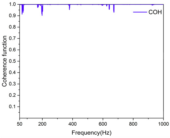
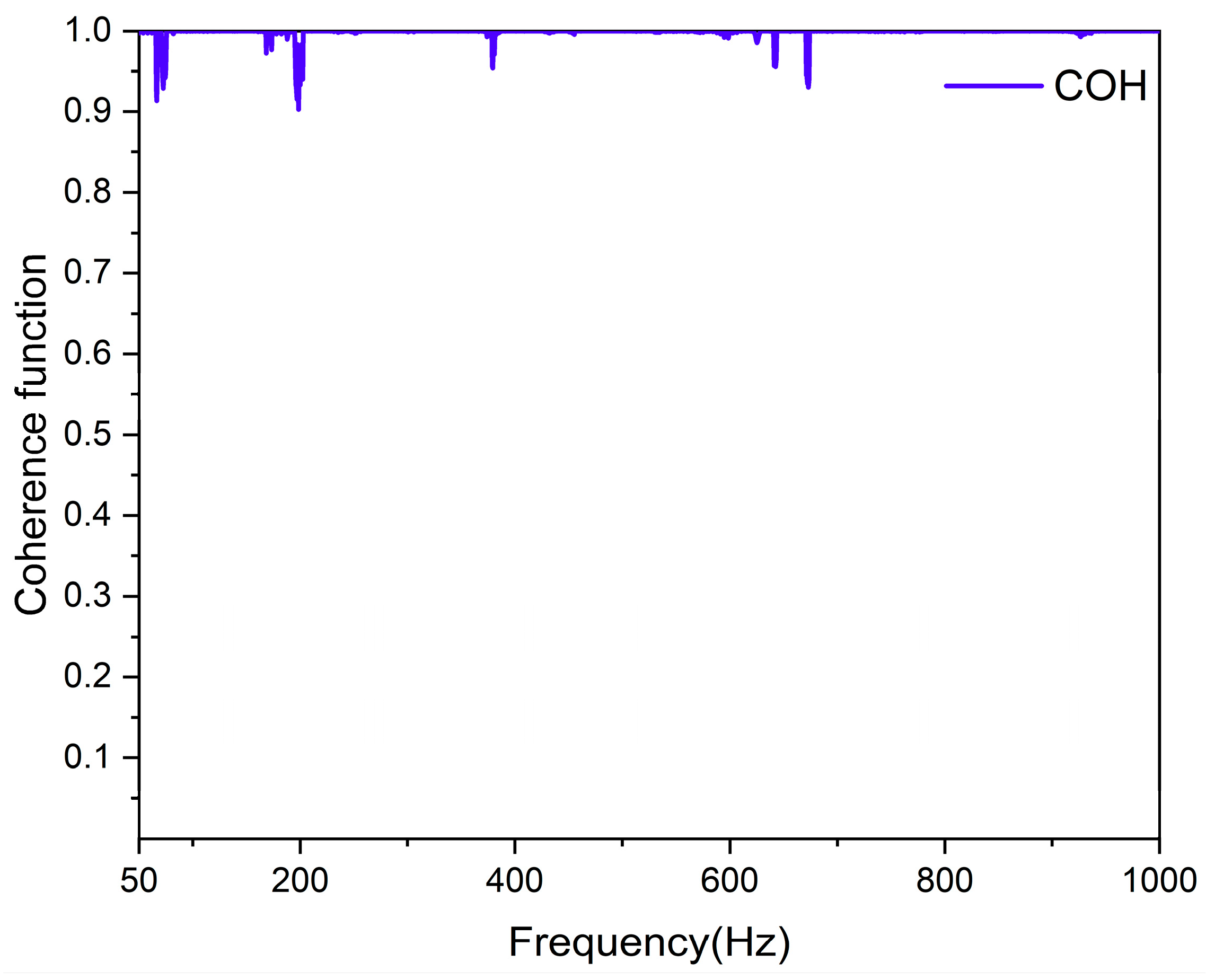
In the equation, $S_{ff}$ is the auto-power spectrum of the excitation, $S_{aa}$ is the auto-power spectrum of the response, and $S_{fa}$ is the cross-power spectrum. ISO 7626-2:2015 [37] specifies a method for measuring linear mechanical mobility and related frequency response functions using a single-point translational exciter, and defines the frequency response function as the ratio of the complex motion response to the complex excitation force in a linear system that varies with frequency. In FRF testing, the coherence function ${\gamma }_{fa}^2$ can be used to evaluate the degree of linear correlation between the excitation and response signals. When ${\gamma }_{fa}^2=1$, the response is completely transmitted through the linear system by excitation, and there is no noise influence. When ${\gamma }_{fa}^2\ll 1$, there may be interference factors such as nonlinear behavior, external noise, measurement error, or channel leakage in the system. Figure 2 shows the coherence function curve of specimen (a) under excitation at 50–1000 Hz.

Figure 2. Coherence function of the frequency response of specimen (a) in the 50–1000 Hz range.

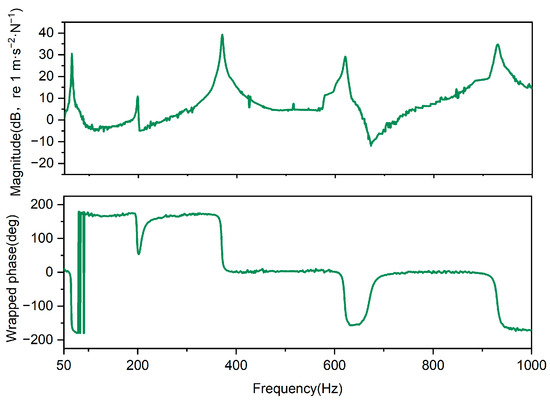
As shown in the figure, ${\gamma }_{fa}^2$ only approaches 0.9 at a few isolated points. In most frequency ranges, the system shows good linearity and a high signal-to-noise ratio. Figure 3 presents the magnitude–frequency plot and the wrapped phase–frequency plot of the frequency response function of the specimen (a) under sinusoidal swept-sine excitation in the range of 50–1000 Hz.

Figure 3. Magnitude and wrapped phase curves of the frequency response function of specimen (a) in the 50–1000 Hz range.

As shown in Figure 3, the specimen (a) exhibits the first five modal poles, with obvious zeros at 198.5 Hz and 620.0 Hz. By using the magnitude and phase information in the Bode plots, calculate the parameters $R_r^{\left(a\right)}$, ${\omega }_r$ and ${\zeta }_r$ of the transfer function, and assemble the expression of the transfer function for the multi-degree-of-freedom vibration system. Table 1 lists the identified transfer-function parameters for Modes 1 to 5.

Table 1. Transfer-function parameters of the first five modes of specimen (a).

Mode Order	Pole (Hz)	Damping Ratio	Undamped Natural Frequency (Rad/s)	Wrapped Phase (Deg)	Magnitude (m/s2/N)
Mode 1	65.0	0.0073	408.43	−85.53	33.42
Mode 2	198.5	0.0062	1247.26	+110.86	3.51
Mode 3	370.5	0.0043	2327.96	+87.07	92.22
Mode 4	620.0	0.0041	3895.64	−77.99	28.66
Mode 5	930.0	0.0046	5843.48	−84.90	54.69

The identified transfer-function parameters can also be interpreted as dynamic characterization indicators of the wooden beam specimens. The resonance frequencies and damping ratios listed in Table 1 are not only fitting parameters, but also modal dynamic parameters in the bending response of the specimen. For lightly damped vibration, the corresponding loss factor can be approximately estimated as ${\eta }_r\approx 2{\zeta }_r$. When the density and geometrical parameters of the beam are known, the identified resonance frequencies can be converted into an apparent bending dynamic modulus based on the Euler–Bernoulli beam relationship. Therefore, the transfer-function model provides a parameterized path for extracting actual dynamic indicators from the measured FRF. These indicators include resonance frequency, damping ratio, loss factor, modal coupling strength, and apparent dynamic modulus.

According to Equation (7), it can be calculated that

$$\begin{array}{l}H\left(s\right)={\displaystyle \frac{8.07\times 10^4+6.31\times 10^3\times \mathrm{j}}{s^2+5.93s+1.67\times 10^5}}+{\displaystyle \frac{-6.33\times 10^4-2.41\times 10^4\times \mathrm{j}}{s^2+15.48s+1.56\times 10^6}}\\ +{\displaystyle \frac{-4.33\times 10^6+2.22\times 10^5\times \mathrm{j}}{s^2+20.18s+5.42\times 10^6}}\\ +{\displaystyle \frac{3.50\times 10^6+7.45\times 10^5\times \mathrm{j}}{s^2+32.08s+1.52\times 10^7}}+{\displaystyle \frac{1.71\times 10^7+1.52\times 10^6\times \mathrm{j}}{s^2+53.35s+3.41\times 10^7}}\end{array}$$

(25)

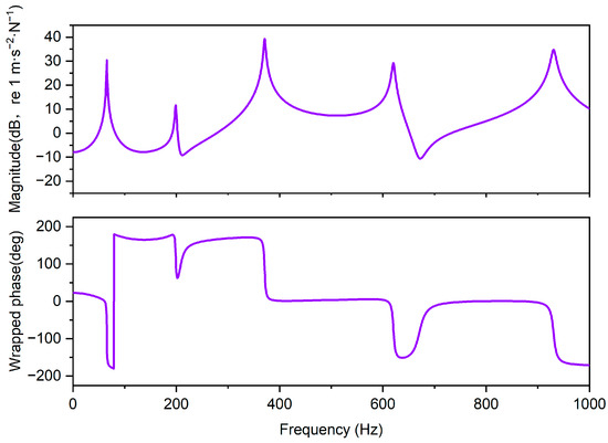
Equation (25) was the expression of the transfer function for the specimen (a) under free–free boundary conditions, with the excitation point at 0.5 L and the response point at 1 L, where $s=\mathrm{j}\omega$ and $\omega =2\pi f$. Figure 4 shows the Bode magnitude plot and wrapped-phase plot of this transfer function for the simulation frequency range of 0–1000 Hz, where the magnitude is represented as $20{\mathrm{l}\mathrm{o}\mathrm{g}}_{10}\mid H\left(j\omega \right)\mid$(dB) and the phase is represented as $\mathrm{a}\mathrm{r}\mathrm{g}\left[H\right(j\omega \left)\right]$.

Figure 4. Simulated magnitude and wrapped-phase curves of the transfer-function model of specimen (a) in the 0–1000 Hz range.

To evaluate the response reconstruction ability of the identified transfer-function model, an additional swept-sine input was used as validation after the model parameters were determined. The validation signal was applied under the same experimental setup, with a frequency range of 50–1000 Hz, a peak-to-peak excitation voltage of 11 V, and an initial phase of 0°. The input force spectrum measured under this validation condition was substituted into Equation (25), and the corresponding acceleration response was calculated in the range of 50–1000 Hz. Compare the predicted with the LDV-measured acceleration response, as shown in Section 3.2.

3. Results and Discussion

Considering the limited number of specimens, the purpose of the present analysis is to verify the feasibility, consistency, and reusability of the proposed transfer-function identification and reconstruction procedure for wooden beam specimens under controlled testing conditions. The analysis focuses on whether the measured force–acceleration FRFs can be converted into physically interpretable and reconstructable modal-parameter representations. In this study, one primary Sitka spruce beam specimen was used for detailed model construction, while two additional specimens were used for consistency validation. Therefore, population-level statistical characterization of Sitka spruce material properties was not conducted.

3.1. Bode Plot Fitting and Error Evaluation

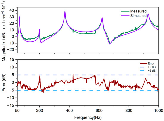
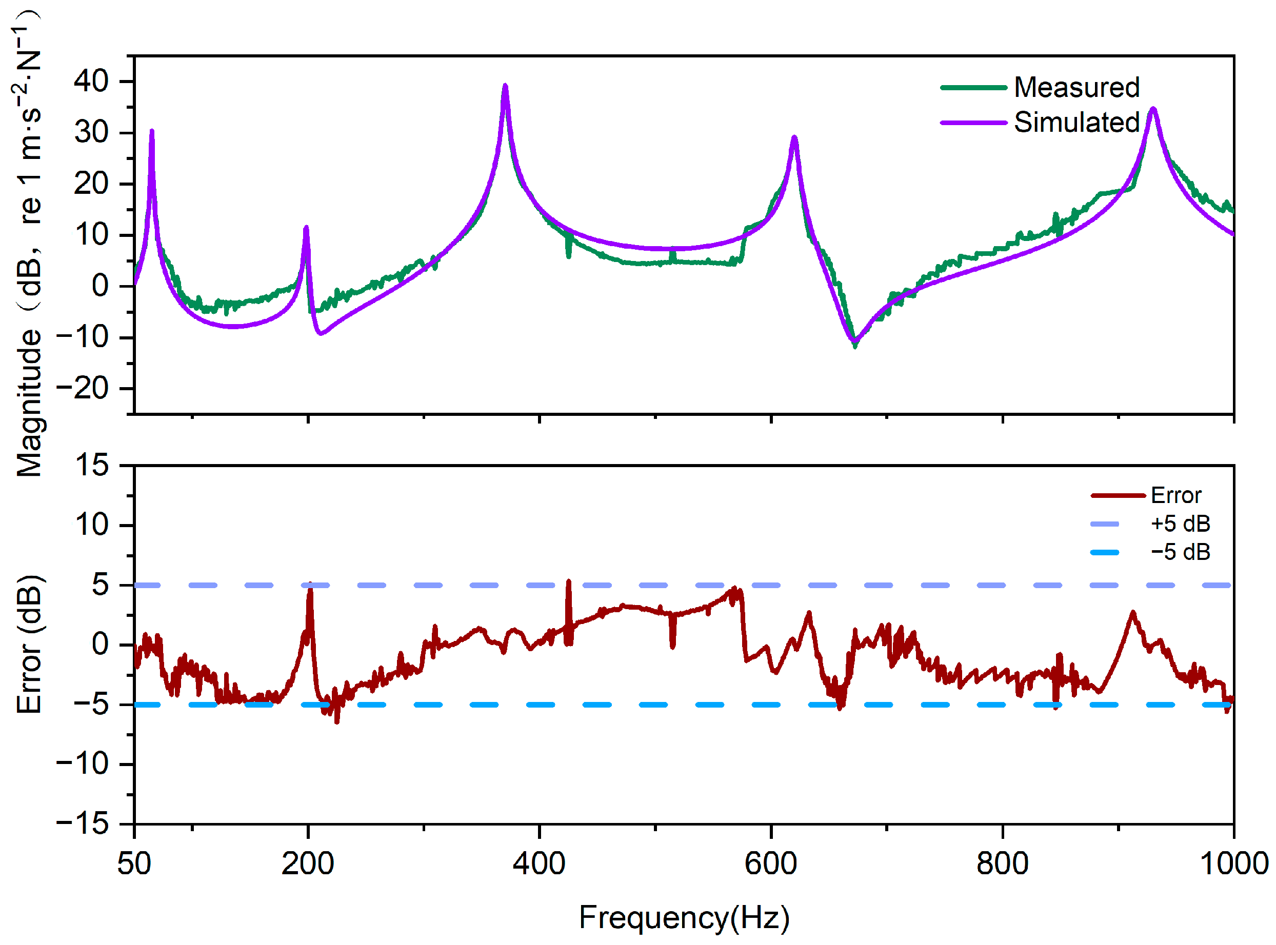
Figure 5 shows the simulated and measured FRF magnitude curves and error of specimen (a). It can be seen that the model is in good agreement with the experimental FRF magnitude. Within the frequency range, the RMSE, MAE, and ME were 2.64 dB, 2.23 dB, and −0.96 dB, respectively, indicating that the model slightly underestimated the experimental results. The five resonance points were located at 65.0 Hz, 198.5 Hz, 370.5 Hz, 620.0 Hz, and 930.0 Hz, with corresponding magnitude errors of −0.034 dB, 0.726 dB, 0.017 dB, 0.080 dB, and 0.007 dB, respectively. Except for the resonance at 198.5 Hz, the error of all other resonance points was less than 0.1 dB, indicating that the model has high reproducibility accuracy for peak position and peak magnitudes of the dominant modes. According to the error-band statistics, 69.65% and 98.58% of the frequency points fell within ±3 dB and ±5 dB, respectively, indicating that the magnitude fitting within the frequency range was reliable.

Figure 5. The simulated and measured FRF magnitude curves and error of specimen (a).

Only 1.42% of the frequency points exceeded the ±5 dB, and these points were mainly concentrated in a few narrow frequency bands near 225.0 Hz, 425.0 Hz, 660.0 Hz, and near 1 kHz, mostly in peak–valley transitions or areas with large local slope. This indicates that the error mainly comes from local frequency offset and damping mismatch, rather than modal deviation. The model performs stability near the main resonance peaks and has good characterization ability for frequency band magnitude response. Previous studies on the vibration of wood and tonewood have usually focused on low-order resonance frequencies, damping-related indicators, or FRF changes based on impact or vibration testing [20,21,22,23]. These studies provided a basis for evaluating the acoustic and dynamic properties of wooden specimens using resonance testing. Compared with the explanations based on peak recognition or FRF changes in these studies, this model in this study reconstructs the magnitude and phase of the measured force–acceleration FRF in the 1st–5th modal range. The model has a small resonance-peak magnitude error and bounded full-band residuals, which can not only identify resonance positions, but also maintain the magnitude evolution near the dominant mode.

Table 2 shows the simulation and measurement phases and errors of the first five poles of specimen (a). The wrapped-phase errors at the five resonance points were 0.20°, 5.08°, 0.34°, 2.85°, and 0.22°, respectively. The mean absolute error was 1.74°, and the maximum absolute error occurred at 198.5 Hz. Except for the second resonance point, the phase errors at all other points were very small, with less than 1° at 65.0 Hz, 370.5 Hz, and 930.0 Hz. The constructed model effectively preserved the phase characteristics near the resonance points and was consistent with experimental results in the phase domain. The model can accurately reproduce the resonance characteristics of the measured FRF and perform parameter identification.

Table 2. Simulation and measurement of zero pole phase error of specimen (a).

	Frequency (Hz)	Measured Phase (Deg)	Simulated Phase (Deg)	Error (Deg)
1st pole	65.0	−85.73	−85.33	0.20
2nd pole	198.5	+110.86	+115.95	5.08
3rd pole	370.5	+87.07	+86.73	0.34
4th pole	620.0	−77.99	−75.14	2.85
5th pole	930.0	−84.90	−84.68	0.22

Approaching the minimum magnitude near the anti-resonance point can cause phase sensitivity to noise. Therefore, the consistency of the zero point was evaluated using the anti-resonance frequency $f_z$ and the notch depth $D_z$, as shown in Table 3. When multiple local anti-resonance valleys appeared within the same pole interval, the zero pairing was determined by the nearest matching rule. Based on the predicted $f_z$ of the model, the nearest local minimum value was selected on the measurement curve as the corresponding zero. In the range of 50–1000 Hz, the model remains consistent in pole and primary anti-resonance.

Table 3. Measured and simulated anti-resonance frequencies and notch depths of specimen (a) in the frequency range of 50–1000 Hz.

Zero	Pole Interval	${\mathit{f}}_{\mathit{z},\mathbf{e}\mathbf{x}\mathbf{p}} \left(\mathbf{H}\mathbf{z}\right)$	${\mathit{f}}_{\mathit{z},\mathbf{m}\mathbf{o}\mathbf{d}} \left(\mathbf{H}\mathbf{z}\right)$	$∆{\mathit{f}}_{\mathit{z}} \left(\mathbf{H}\mathbf{z}\right)$	${\mathit{d}}_{\mathit{e}\mathit{x}\mathit{p}} \left(\mathbf{d}\mathbf{B}\right)$	${\mathit{d}}_{\mathit{m}\mathit{o}\mathit{d}} \left(\mathbf{d}\mathbf{B}\right)$	$∆\mathit{d} \left(\mathbf{d}\mathbf{B}\right)$
Z1	65.0–198.5	129.5	135.5	−6.0	26.06	28.86	−2.80
Z2	198.5–370.5	204.5	211.5	−7.0	30.04	34.64	−4.60
Z3	370.5–620.0	504.0	511.0	−7.0	30.14	26.94	+3.20
Z4	620.0–930.0	672.5	672.0	+0.5	43.82	42.56	+1.27

$f_z$ is represented as follows:

$$f_z={argmin}_{f\in [f_r,f_{r+1}]}|H(f){|}_{dB}$$

(26)

Here, $f_r$ and $f_{r+1}$ are the two adjacent resonance frequencies enclosing the anti-resonance valley; $\mid H\left(f\right){\mid }_{dB}$ is the FRF magnitude expressed in dB; and $\mathrm{a}\mathrm{r}\mathrm{g}\mathrm{m}\mathrm{i}\mathrm{n}$ returns the frequency $f$ at which $\mid H\left(f\right){\mid }_{dB}$ reaches its local minimum within the interval $\left[f_r,f_{r+1}\right]$. The minimum value is represented as

$$H_{min}=\left|H\right(f_z){|}_{dB}$$

(27)

$H_{min}$ is the minimum dB magnitude of the FRF at the identified anti-resonance frequency $f_z$. The notch depth $D_z$ is defined as

$$D_z={\displaystyle \frac{H_{\mathrm{peak},L}+H_{\mathrm{peak},R}}{2}}-H_{\min }$$

(28)

In this equation, $H_{\mathrm{peak},L}$ and $H_{\mathrm{peak},R}$ are the local peak magnitudes on the left and right sides of the anti-resonance valley, respectively. A larger $D_z$ indicates a deeper anti-resonance notch and stronger local magnitude cancellation, where

$$H_{\mathrm{peak},L}={max}_{f\in [f_r,f_z]}|H(f){|}_{dB}$$

(29)

$$H_{\mathrm{peak},R}={max}_{f\in [f_z,f_{r+1}]}|H(f){|}_{dB}$$

(30)

In Equations (29) and (30), $H_{\mathrm{peak},L}$ is obtained as the maximum dB magnitude in the interval from $f_r$ to $f_z$, whereas $H_{\mathrm{peak},R}$ is obtained as the maximum dB magnitude in the interval from $f_z$ to $f_{r+1}$. The operator $\mathrm{m}\mathrm{a}\mathrm{x}$ returns the maximum value of $\mid H\left(f\right){\mid }_{dB}$ within the specified interval.

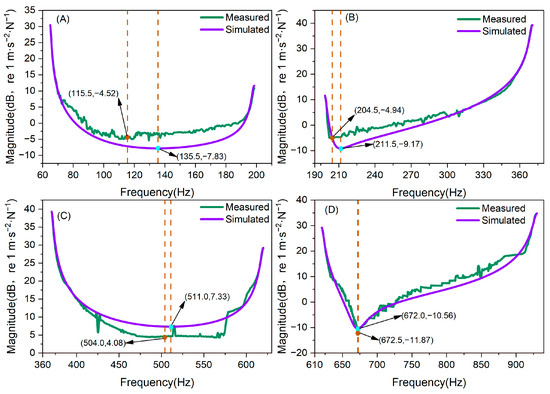
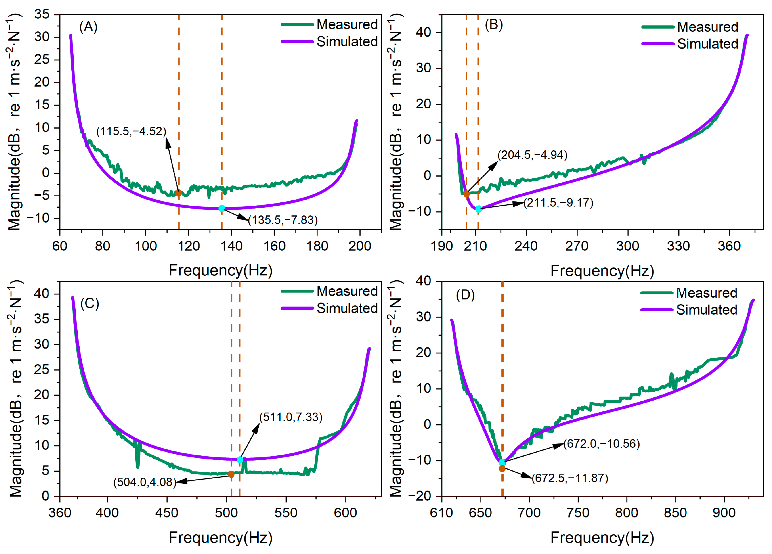
Within the frequency range of 50–1000 Hz, the anti-resonance identification results based on pole-interval segmentation show that the transfer-function model can well reproduce the main zero of the measured FRF. The zero-frequency errors of the four anti-resonance intervals were −6.0 Hz, −7.0 Hz, −7.0 Hz, and +0.5 Hz, respectively, indicating that the model has good predictive ability for anti-resonance positions. The corresponding notch-depth errors were −2.80 dB, −4.60 dB, +3.20 dB, and +1.27 dB, respectively, showing that the model can also well describe the depth of the anti-resonance valley.

Figure 6 shows the partially enlarged views of the anti-resonance interval of specimen (a). The model slightly overestimated the notch depth in Z1 and Z2 and slightly underestimated the notch depth in Z3. The zero position and notch depth of Z4 were very close to the experimental results in this model. The model maintained good consistency in zero localization of all four anti-resonance intervals, and the study used the zero frequency and notch depth as references to evaluate anti-resonance consistency. The results indicate that the model can serve as a relatively reliable reference FRF in the frequency range of 50–1000 Hz.

Figure 6. Partially enlarged views of the anti-resonance interval of specimen (a): (A) Interval Z1; (B) interval Z2; (C) interval Z3; (D) interval Z4.

3.2. Comparison of Time-Domain Responses

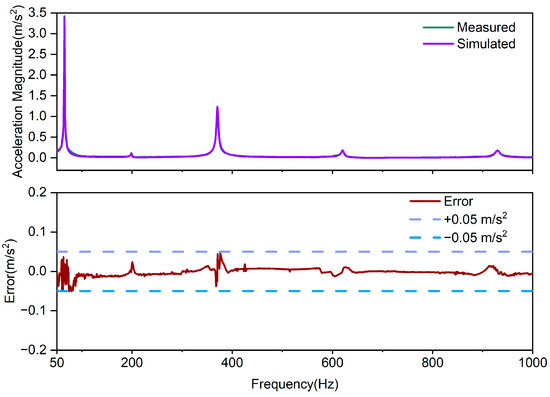
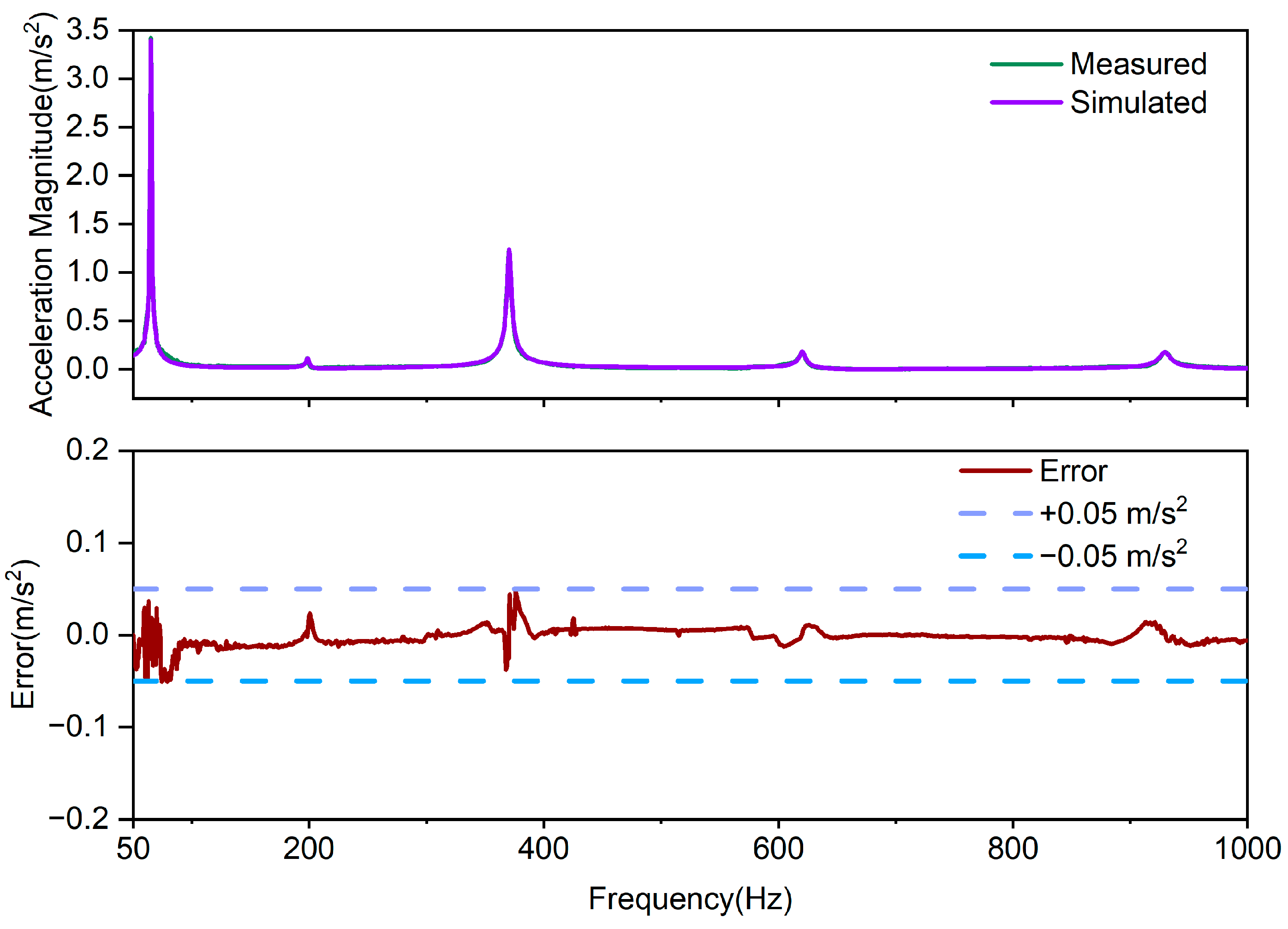
As shown in Figure 7, at the five main resonance peaks shown in the figure, the errors were very small overall. Only the peak at 198.5 Hz showed a slightly larger relative error, mainly because its magnitude was relatively small. Over the full frequency range, the root mean square error (RMSE) of the magnitude error was $9.76\times {10}^{-3} \mathrm{m}/{\mathrm{s}}^2$, the meaning absolute error (MAE) was $6.85\times {10}^{-3} \mathrm{m}/{\mathrm{s}}^2$, and the maximum absolute error was $5.096\times {10}^{-2} \mathrm{m}/{\mathrm{s}}^2$. Approximately 99.9% of the frequency-point errors fell within the reference range of $\pm 5.0\times {10}^{-2} \mathrm{m}/{\mathrm{s}}^2$, and the coefficient of determination reached $R^2=9.961\times {10}^{-1}$. This indicates that the model provides high fitting accuracy and good predictive performance for the actual acceleration magnitude. This response reconstruction result is consistent with the general purpose of modal testing and system identification, and the identified modal model should be able to reconstruct the system response under given input conditions [11,13]. In the acoustic and vibration modeling of wood–based materials, previous studies have also used measured FRF as a calculation input or calibration references [14,24]. The identified transfer-function model in this study can not only serve as an input–output expression, but also be used to predict acceleration responses under new swept-sine force input conditions.

Figure 7. Comparison of measured and simulated acceleration magnitudes of specimen (a) and their error.

3.3. Nyquist Verification

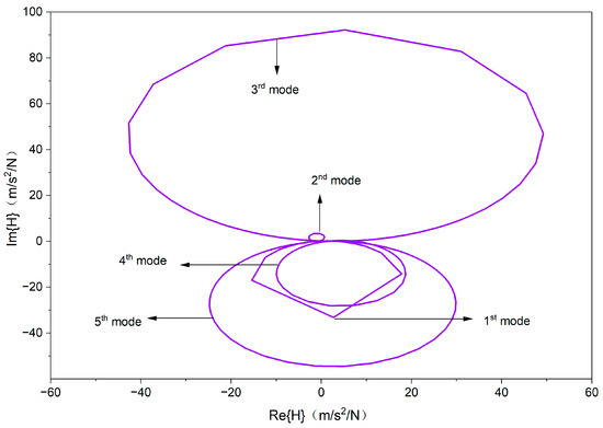
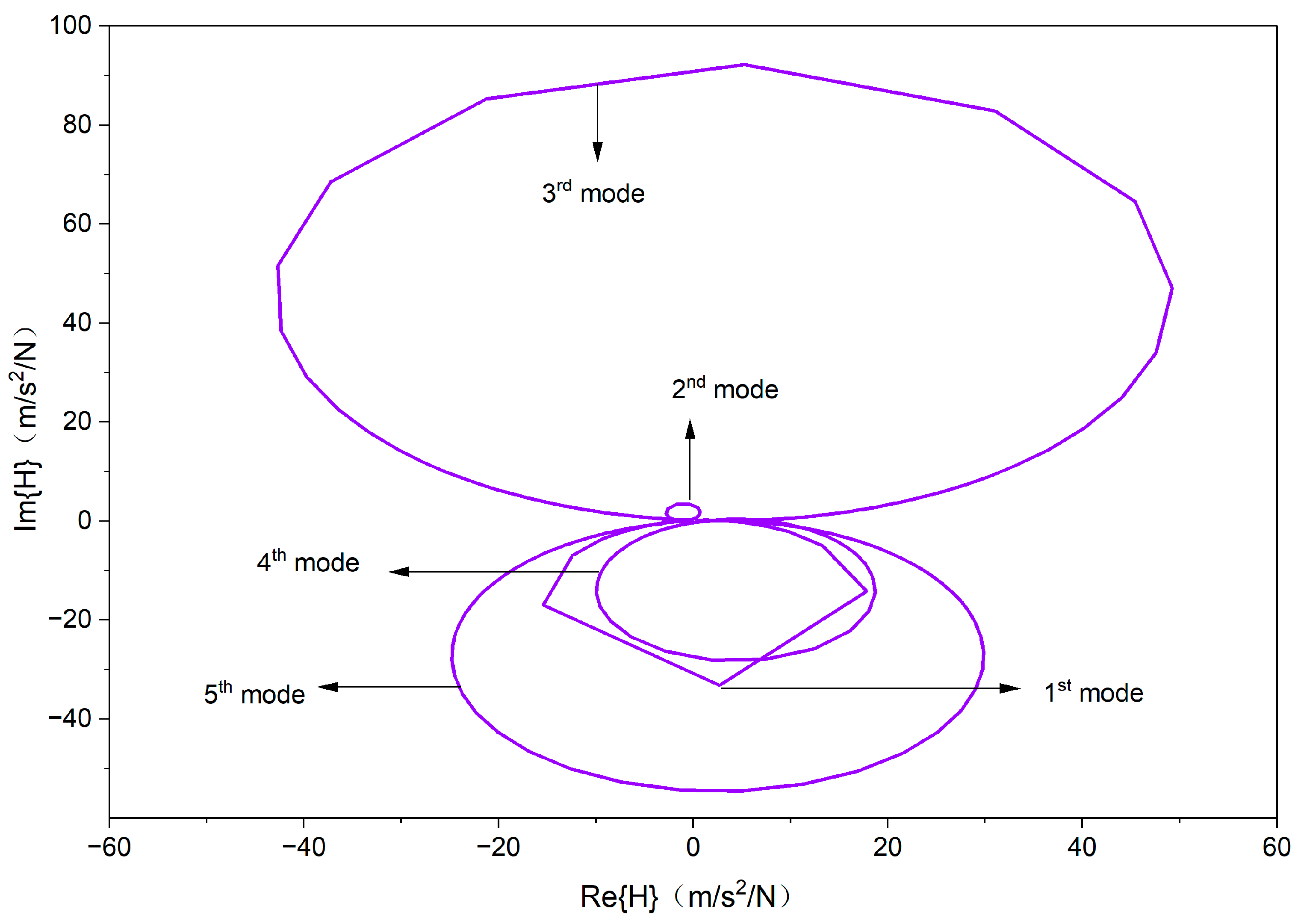
Figure 8 shows the Nyquist trajectory of the specimen (a) transfer function calculated according to Equation (25) in the range of 0–1000 Hz. The Nyquist curve of the model exhibited five clear modal loops and four necked anti-resonance points in the complex-plane trajectory as the frequency increases. The curve was continuous and smooth, without breakpoints or spikes, and the complex calculations including the real and imaginary parts are numerically self-consistent. The curve started near the first quadrant (Re = 0.373, Im = 0.157) and then entered a series of loop segments associated with the first several modes. The relationship between the characteristics of curves and modal features is as follows:

Figure 8. Simulated Nyquist plot of the frequency response function of specimen (a) in the 0–1000 Hz range.

(1) The “loop radius” at each pole corresponds to the strength of the resonance magnitude, and the third mode loop is the most prominent.

The number of loops is equal to the number of resonance modes. For the second-order linear mode, the complex mobility around ${\omega }_r$ is associated with conjugate pole–zero pairs, and each pole pair generates a closed loop around the origin in the complex-frequency domain. Due to the five pole pairs in the model, the Nyquist plot shows five closed loops with five main resonance loops at 65.0, 198.5, 370.5, 620.0, and 930.0 Hz, respectively. Among them, the third resonance point reaches the largest imaginary magnitude in the complex plane $\left(\mathrm{I}\mathrm{m}=+92.24\right)$, while the real part also shows significant positive–negative oscillations in this frequency region (Re varies from $-42.68$ to $\left.+49.21\right)$. This indicates that the third mode has the strongest coupling between the excitation point and the response point and is the dominant radiation/response mode of the structure under measurement.

The second resonance has the smallest loop, with a resonance magnitude of 3.82 m/s²/N. This suggests that the mode multiplication or participation factor of the second mode is weak. Although its damping is not the maximum, it is difficult to form a significant peak, which is consistent with the weak second peak observed in the magnitude response. Expanding the response to the first-order term of the damping ratio, the “radius” of each Nyquist loop can be approximated as ${\varphi }_{jr}{\varphi }_{kr}/2{\zeta }_r$. This also explains why the third loop is the largest, corresponding to the main radiation region. The second loop is the smallest, which means $\mid {\varphi }_{jr}{\varphi }_{kr}\mid$ is minimal for the selected excitation–response point combination.

(2) The anti-resonance points are the “necking” of the complex-plane trajectory towards the origin, and the depth of the notch can be seen.

There are four distinct necking regions on the curve near 135.5, 211.5, 511.0, and 672.0 Hz. Among them, the trajectory at 672.0 Hz is closest to the origin $\left(\mathrm{R}\mathrm{e}=0.086,\mathrm{I}\mathrm{m}=-0.284\right)$, with the strongest zero cancellation and the deepest notch. The regions at 135.5 Hz and 211.5 Hz are also close to origin, with magnitudes of 0.406 and 0.348, respectively, and can therefore be considered as typical deep anti-resonance valleys. The necking radius of 511.0 Hz is larger, with a magnitude of 2.33, corresponding to a shallow valley. This is consistent with the experimental observation that the anti-resonance valleys are not equally deep. However, the trajectories at these zeros will not pass through the origin but only approach it. This is consistent with the common situation where the real frequency zero point does not need to be strictly zero when damping and residual terms exist.

(3) The alternating quadrants of the loops reflect the phase rule of approximately ±90° near resonance. The symbol change comes from zeros and measurement-point coupling, rather than an anomaly.

At the five resonance points, the phase values are within ±(75–116°). The phases of the first, third, fourth, and fifth modes are −85°, +87°, −75°, and −85°, respectively. The second mode has a negative real part and positive imaginary part, so the point is located in the second quadrant, corresponding to a phase of +116°. This alternation of quadrants usually means that in different modal ranges, the signs of the real and imaginary parts of the complex response are jointly controlled by the product of the zero point and the mode shape. Especially when the excitation and response points are not completely coincident, it is normal for some modal segments to fall into the second or fourth quadrant. This does not imply that the system is physically invalid.

(4) At the high frequencies, the trajectory tends toward the third quadrant and gradually approaches the real axis, which is the combined influence of residual terms and the tails of higher-order modes.

After 930.0 Hz, the Nyquist curve gradually converges to the region where the real part is negative and the absolute value of the imaginary part decreases $\left(\mathrm{R}\mathrm{e}=-3.17, \mathrm{Im}=-0.52\right.$ near 1000.0 Hz). This is because at high frequencies, the direct peak contributions of low-order modes weaken, while the combined influence of the residual terms and the tails of higher-order modes gradually increases.

The Nyquist plot of the proposed model presents five main loops and four anti-resonance necking regions in the complex plane, which is consistent with the pole–zero structure. The third loop is significantly enlarged while the second loop is clearly contracted, reflecting the combined effects of excitation–response point coupling and damping modulation on the resonance magnitude. The necking points approach the origin but do not pass through it, which is consistent with anti-resonance characteristics under damping and residual effects, that is, “near zero rather than completely zero”.

Compared with previous studies on resonance frequency or damping ratio, Nyquist plots and pole-position results can provide additional information. Studies on modal-identification of wooden components have shown that the identified modal parameters may be affected by boundary conditions, signal-to-noise ratio, and post-processing algorithms [10,11,12,13]. The continuous Nyquist trajectory and the left-half-plane pole distribution obtained in this study provide a complex-domain verification basis for identifying the stability and consistency of the model. This research has shown that in evaluating the modal characterization of wooden beam specimens based on FRF, Bode magnitude, phase, Nyquist trajectory, and pole parameters should be comprehensively considered.

3.4. Phase Characteristics and Pole–Zero Patterns

Poles correspond to the structural modes of the system, and zeros are transfer zeros related to the input and output locations. When the denominator $-{\omega }^2+2\mathrm{j}{\zeta }_r{\omega }_r\omega +{\omega }_r^2$ of Equation (8) approaches zero, the acceleration magnitude tends to peak. When $\omega \approx {\omega }_r$, the modulus of the denominator is the minimum value, corresponding to the pole, which is the resonance point.

Within each interval between two adjacent poles $\left({\omega }_r,{\omega }_{r+1}\right)$, the sign variations of $H_R$ and $H_I$ can be used to analyze the evolution of the complex-response direction and the trajectory in the complex plane. If an obvious sign reversal or quadrant transition occurs within a given interval, this usually indicates the possible presence of an antiresonance valley or a near-zero feature in that interval. However, whether such a feature can be identified as a zero should still be determined ultimately by examining whether $\mid H\left(f\right)\mid$ exhibits an interior local minimum within the same interval. Writing the residue of each mode in the form $a_r+\mathrm{j}{b}_r$, where $a_r$ and $b_r$ are the real and imaginary parts of the modal residue, respectively, Equation (8) can be rewritten as

$$H\left(\mathrm{j}\omega \right)=H_R+\mathrm{j}{H}_I$$

(31)

where $H_R$ and $H_I$ are the real and imaginary parts of the complex frequency response function $H\left(\mathrm{j}\omega \right)$, respectively, where

$$H_R(\omega )={\sum }_{r=1}^5{\displaystyle \frac{\left(a_r\right)({\omega }_r^2-{\omega }^2)+2{\zeta }_r{\omega }_r\omega b_r}{({\omega }_r^2-{\omega }^2{)}^2+(2{\zeta }_r{\omega }_r\omega {)}^2}}$$

(32)

$$H_I(\omega )={\sum }_{r=1}^5{\displaystyle \frac{\left(b_r\right)({\omega }_r^2-{\omega }^2)-2{\zeta }_r{\omega }_r\omega a_r}{({\omega }_r^2-{\omega }^2{)}^2+(2{\zeta }_r{\omega }_r\omega {)}^2}}$$

(33)

Equations (32) and (33) separate the fitted transfer function into real and imaginary components, allowing the sign changes of $H_R$ and $H_I$ to be related to quadrant transitions in the Nyquist trajectory. By using Equation (31) to calculate, Table 4 was obtained to determine the position of the zeros. The anti-resonance points were identified based on the local minimum $\mid H\left(f\right)\mid$ of each interval between two adjacent poles. The sign reversals of $H_R$ and $H_I$ are used only to assist in explaining the change in the complex response directions and the formation of the anti-resonance valley and are not the only method for identifying anti-resonance points. The results correspond to those shown in Figure 4.

Table 4. Determination of the zero points position of the transfer function of specimen (a).

Interval (Hz)	Sign of ${\mathit{H}}_{\mathit{R}}$	Sign of ${\mathit{H}}_{\mathit{I}}$	Complex Quadrant Transition	Result
65.0~198.5	$-$	$-\to +$	$\mathrm{III}\to \mathrm{II}$	One zero (135.5 Hz)
198.5~370.5	$-\to +\to -$	$+$	$\mathrm{II}\to \mathrm{I}\to \mathrm{II}$	One zero (211.5 Hz)
370.5~620.0	$+$	$+\to -$	$\mathrm{I}\to \mathrm{IV}$	One zero (511.0 Hz)
620.0~930.0	$+\to -\to +$	$-\to +\to -$	$\mathrm{IV}\to \mathrm{III}\to \mathrm{IV}\to \mathrm{I}\to \mathrm{IV}$	One zero (672.0 Hz)
930.0~1000.0	$-$	$-$	$\mathrm{III}$	No zero

Wood with high moisture content has relatively high internal friction. Its resonance peaks are usually low and wide, and the peak positions cannot be accurately identified from the FRF magnitude curve. In contrast, the points where the phase crosses ±90° are almost unaffected by magnitude attenuation and can serve as reliable indicators of resonance. The wrapped phase in the Bode plot can be used to distinguish the modal direction. In the force–acceleration FRF, ${\varphi }_{jr}{\varphi }_{kr}>0$ represents that the excitation point and the response point move in the same direction, and ${\varphi }_{jr}{\varphi }_{kr}<0$ represents that they move in opposite directions.

According to Figure 4, the pole phases are mainly distributed around ±90°, and the phases near the zeros appear around 0°, ±180°, or in some cases around ±90°.

When $s=\mathrm{j}\omega$, Equation (3) can be decomposed into a single-degree-of-freedom form:

$$H_{disp}^{\left(r\right)}({\omega }_r)={\displaystyle \frac{R_r^{\left(x\right)}}{{\omega }_r^2-{\omega }^2+2\mathrm{j}{\zeta }_r{\omega }_r\omega }}$$

(34)

where $H_{disp}^{\left(r\right)}(\mathrm{j}\omega )$ is the displacement-to-force FRF contribution of the $r$-th single modal component evaluated on the imaginary axis. The numerator is $R_r^{\left(x\right)}={\varphi }_{jr}{\varphi }_{kr}$. After modal orthonormalization, the mode shape ${\varphi }_r\left(x\right)$ can be regarded as purely real. When $\omega ={\omega }_r$, the denominator ${\omega }_r^2-{\omega }^2+2\mathrm{j}{\zeta }_r{\omega }_r\omega$ becomes $2\mathrm{j}{\zeta }_r{\omega }_r^2,$ that is,

$$\mathrm{\angle }{H}_{disp}^{\left(r\right)}\left(\mathrm{j}{\omega }_r\right)=\mathrm{\angle }{R}_r^{\left(x\right)}-{90}^{°}=\left\{\begin{array}{c}-90°,R_r^{\left(x\right)}>0\\ +90°,R_r^{\left(x\right)}<0\end{array}\right.$$

(35)

The sign $\pm$ depends on $R_r^{\left(x\right)}$. If the signs of ${\varphi }_{jr}{\varphi }_{kr}$ are the same, then $R_r^{\left(x\right)}>0$, and the phase is $-{90}^{\circ }$. Otherwise, $R_r^{\left(x\right)}<0$, and the phase is $+{90}^{\circ }$.

${\varphi }_{jr}{\varphi }_{kr}$ is the intrinsic modal characteristic of the system. It represents the relative vibration–displacement pattern of each point on the specimen in the $r$-th mode. For wooden beam under free–free boundary conditions, the mode shape ${\varphi }_r\left(x\right)$ can be derived using the Euler–Bernoulli beam theory, and its real-valued form is as follows [38,39,40].

$${\varphi }_r(x)={\mathit{sin}\beta }_{r}x+{\mathit{sin}h\beta }_{r}x+{\displaystyle \frac{{\mathit{sin}\beta }_{r}L-{\mathit{sin}h\beta }_{r}L}{{\mathit{cos}h\beta }_{r}L-{\mathit{cos}\beta }_{r}L}}({\mathit{cos}\beta }_{r}x+{\mathit{cos}h\beta }_{r}x)$$

(36)

where ${\varphi }_r\left(x\right)$ is the real-valued mode-shape function of the $r$-th bending mode along the beam length, $x$ is the longitudinal coordinate, $L$ is the beam length, and ${\beta }_r$ is the modal wavenumber. Here, ${\beta }_{r}L$ is the $r$-th root of the equation $1=\mathrm{c}\mathrm{o}\mathrm{s}\left({\beta }_{r}L\right)\mathrm{c}\mathrm{o}\mathrm{s}\mathrm{h}\left({\beta }_{r}L\right)$, (1 → 4.730, 2 → 7.853, 3 → 10.996…), and then the signs at the excitation point $0.5 \mathrm{L}$ and the response point $1 \mathrm{L}$ were then determined accordingly [41].

Table 5 presents the sign of the mode-shape functions at the excitation and the response point, as well as the sign of their product. For a free–free beam, the even-order mode shapes around the center $0.5 \mathrm{L}$ are antisymmetric, so the displacement directions at the left and right ends must be opposite. This is an inherent symmetry of the mode shapes. Due to the excitation at the center ($0.5 \mathrm{L}$), the modal shape indicates that when $r$ is even, this position is theoretically a node, ${\varphi }_{kr}=0$. In numerical calculation, only a very small value is generated, so the sign of the even-order term cannot be determined theoretically. However, in the experiment, the excitation point cannot be accurately located at $0.5 \mathrm{L}$, and a slight offset can cause the even-order modes to display phases around $\pm {90}^{\circ }$.

Table 5. Signs of the mode shapes and product at the excitation and response points.

Mode Order r	${\mathit{\varphi }}_{\mathit{j}\mathit{r}}={\mathit{\varphi }}_{\mathit{r}} \left(0 \mathbf{L}\right)$	${\mathit{\varphi }}_{\mathit{k}\mathit{r}}={\mathit{\varphi }}_{\mathit{r}} \left(0.5 \mathbf{L}\right)$	${\mathit{\varphi }}_{\mathit{j}\mathit{r}}={\mathit{\varphi }}_{\mathit{r}} \left(1 \mathbf{L}\right)$	Product ${\mathit{\varphi }}_{\mathit{j}\mathit{r}}{\mathit{\varphi }}_{\mathit{k}\mathit{r}}$
1	$-$	$+$	$-$	$-$
2	$-$	Node	$+$	Node
3	$-$	$-$	$-$	$+$
4	$-$	Node	$+$	Node
5	$-$	$+$	$-$	$-$

$R_r^{\left(x\right)}$ is the displacement residue, which needs to be multiplied by $s^2$ to convert it into an acceleration residue. According to Equation (6), the Bode phase of the force–acceleration relationship is obtained by adding ${180}^{\circ }$ to the phase of the force–displacement relationship. Therefore, $+{90}^{\circ }+{180}^{\circ }=+{270}^{\circ }$, and this phase is equivalent to $-{90}^{\circ }$. Similarly, $-{90}^{\circ }+{180}^{\circ }=+{90}^{\circ }$. It can be inferred that the excitation point is located on the $0.5 \mathrm{L}\to 0 \mathrm{L}$ side.

In theory, the frequency response function (FRF) in the resonance region is dominated by a single second-order term. However, in practice, modal overlap or higher-order residual contributions often exist, which combine into a complex vector near the resonance point.

When a pair of adjacent modes, $r$ and $r+1$, is dominant, the contributions of the other terms may be neglected, resulting in

$$H_{acc}(\mathrm{j}\omega )\approx {\displaystyle \frac{R_r^{\left(a\right)}}{{\omega }_r^2-{\omega }^2}}+{\displaystyle \frac{R_{r+1}^{\left(a\right)}}{{\omega }_{r+1}^2-{\omega }^2}}$$

(37)

Let $\omega ={\omega }_{ar}$, where ${\omega }_{ar}$ is the angular anti-resonance frequency corresponding to $f_z$, namely ${\omega }_{ar}=2\pi f_z$. By setting the real part equal to zero, one obtains

$${\displaystyle \frac{R_r^{\left(a\right)}}{{\omega }_r^2-{\omega }_{ar}^2}}+{\displaystyle \frac{R_{r+1}^{\left(a\right)}}{{\omega }_{r+1}^2-{\omega }_{ar}^2}}=0\Rightarrow {\omega }_{ar}^2={\displaystyle \frac{R_r^{\left(a\right)}{\omega }_r^2+R_{r+1}^{\left(a\right)}{\omega }_{r+1}^2}{R_r^{\left(a\right)}+R_{r+1}^{\left(a\right)}}}$$

(38)

Substituting Equation (38) into Equation (37) gives

$$H(\mathrm{j}{\omega }_{ar})={\displaystyle \frac{R_r^{\left(a\right)}+R_{r+1}^{\left(a\right)}}{\left({\omega }_r^2-{\omega }_{ar}^2\right)\left({\omega }_{r+1}^2-{\omega }_{ar}^2\right)}}$$

(39)

The numerator is simplified as $R_r^{\left(a\right)}+R_{r+1}^{\left(a\right)}$. If the directions of these two vectors are opposite, their sum becomes very small, so $\mid H\left(\mathrm{j}{\omega }_{ar}\right)\mid$ is small and the notch is deep. If they are in the same direction, the result is close to the sum of their magnitudes, so $\mid H\left(\mathrm{j}{\omega }_{ar}\right)\mid$ is larger and the notch is shallower.

$$|H(\mathrm{j}{\omega }_{ar})|={\displaystyle \frac{\left|R_r^{\left(a\right)}+R_{r+1}^{\left(a\right)}\right|}{\left|{\omega }_r^2-{\omega }_{ar}^2\right|\left|{\omega }_{r+1}^2-{\omega }_{ar}^2\right|}}$$

(40)

At $\omega ={\omega }_{ar}$, the term $\mid {\omega }_r^2-{\omega }_{ar}^2\mid \mid {\omega }_{r+1}^2-{\omega }_{ar}^2\mid$ is a fixed real number. It only depends on the position of the two poles and is no longer related to the magnitude or phase of the residues. Using $\mid R_r+R_{r+1}\mid$ for direct comparison would still be affected by the relative strength of the two modes themselves. Therefore, a normalization factor is introduced as follows:

$$C={\displaystyle \frac{|R_r+R_{r+1}|}{\left|R_r\right|+\left|R_{r+1}\right|}}\in [\mathrm{0,1}]$$

(41)

where $C$ is the normalized vector-sum coefficient of the two adjacent modal residues. It is used to quantify the cancellation degree between the two residue vectors: a smaller $C$ represents stronger vector cancellation, while a larger $C$ represents weaker cancellation. In this way, the results of the two vectors are compared with the sum of their individual lengths. When $C\to 0$, the directions of these two vectors are opposite, and the two adjacent modes produce strong cancellation, resulting in an infinitely deep notch, or valley. When $C\approx 1$, the two vectors are in the same direction, and the two adjacent modes only produce weak cancellation, so the notch is only slightly lower than the adjacent peaks, corresponding to a shallow valley.

By simplifying Equation (39), the following is obtained:

$$H(\mathrm{j}{\omega }_{ar})={\displaystyle \frac{N_R+\mathrm{j}{N}_I}{D}}$$

(42)

where

$$N_R=R_r^{\left(a\right)}+R_{r+1}^{\left(a\right)}$$

(43)

$$N_I=2{\omega }_{ar}\left({\displaystyle \frac{{\zeta }_r{\omega }_r{R}_r}{{\omega }_r^2-{\omega }_{ar}^2}}+{\displaystyle \frac{{\zeta }_{r+1}{\omega }_{r+1}{R}_{r+1}}{{\omega }_{r+1}^2-{\omega }_{ar}^2}}\right)$$

(44)

$$D=({\omega }_r^2-{\omega }_{ar}^2)({\omega }_{r+1}^2-{\omega }_{ar}^2)$$

(45)

where $N_R$ and $N_I$ are the real and imaginary components of the equivalent numerator at the anti-resonance angular frequency ${\omega }_{ar}$, respectively, and $D$ is the real denominator determined by the frequency distances between ${\omega }_{ar}$ and the two adjacent modal frequencies. The phase at the anti-resonance point is given by

$${\phi }_{ar}=\mathit{arg}\left(H\left(\mathrm{j}{\omega }_{ar}\right)\right)=\mathit{arg}\left(N_R+\mathrm{j}{N}_I\right)=\mathit{atan}2(N_I,N_R)$$

(46)

where ${\phi }_{ar}$ is the phase angle of the FRF at the anti-resonance angular frequency ${\omega }_{ar}$. The function $\mathrm{a}\mathrm{t}\mathrm{a}\mathrm{n}2(N_I,N_R)$ calculates the phase angle based on the signs of $N_R$ and $N_I$, while maintaining the correct quadrant. When $\mid N_I\mid \ll \mid N_R\mid$, the notch is shallow and the real part is dominant, so ${\varphi }_{ar}=0^{\circ }$ or $\pm {180}^{\circ }$. In this case, a positive real value corresponds to $0^{\circ }$, while a negative real value corresponds to $+{180}^{\circ }$. When $\mid N_I\mid \approx \mid N_R\mid$, the real and imaginary parts have the same order, and ${\varphi }_{ar}=\pm {45}^{\circ }$ or $\pm {135}^{\circ }$. When $\mid N_I\mid \gg \mid N_R\mid$, the notch is deeper and the imaginary part is dominant. In this case, the sign is determined by $N_I$, and ${\varphi }_{ar}=\pm {90}^{\circ }$.

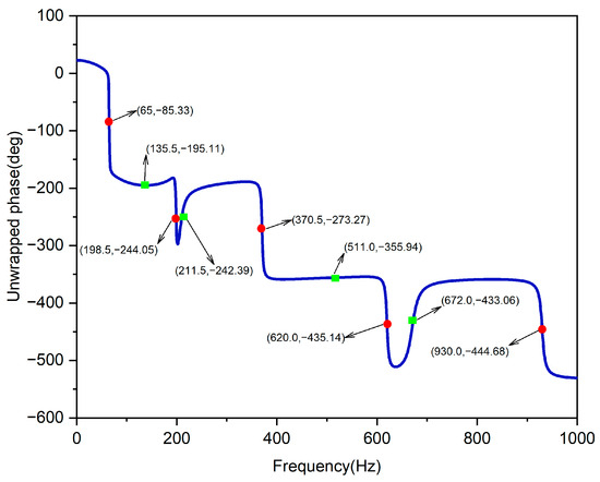
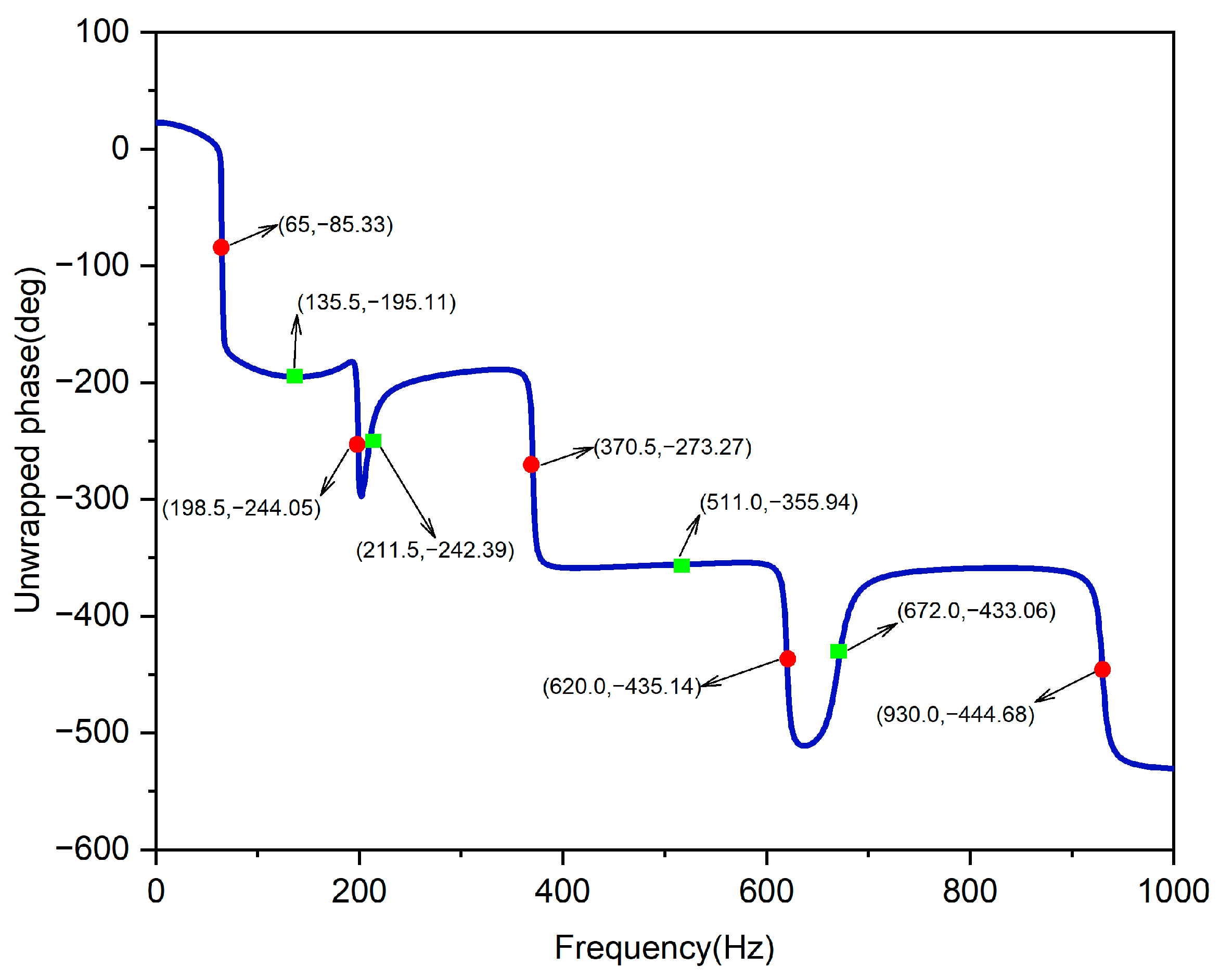
As shown in Figure 4, the simulated magnitude response and wrapped phase curve of the transfer-function model reveal two shallow notches and two deep notches, all of which correspond to trajectories in the Nyquist plot that contract towards the origin. Among them, the notches at 135.5 Hz and 511.0 Hz are relatively shallow, with phase values of $+{164.89}^{\circ }$ and $+{4.06}^{\circ }$, respectively, consistent with the phase pattern of shallow notches. The notches at 211.5 Hz and 672.0 Hz are deep, with phase values of $+{117.61}^{\circ }$ and $-{73.06}^{\circ }$, respectively, consistent with the phase pattern of deep notches. Expand the wrapped phase of the transfer-function Bode plot to obtain the unwrapped-phase curve of the transfer function, as shown in Figure 9.

Figure 9. Unwrapped-phase curve of the simulated frequency response function of specimen (a) in the range of 0–1000 Hz.

The unwrapped-phase curve shows a typical “gradual downward shifts and local rebound.” In several narrow bands, the phase rapidly decreases, corresponding to pole-dominated behavior near resonance. In other bands, the phase forms plateaus or local rise, which is mostly related to anti-resonance cancellation of zeros and the superposition of adjacent modes. The marked points in the figure represent the main phase transition points, which are the resonance-dominated regions near 65.0 Hz, 198.5 Hz, 370.5 Hz, 620.0 Hz, and 930.0 Hz, as well as the anti-resonance-dominated regions near 135.5 Hz, 211.5 Hz, 511.0 Hz, and 672.0 Hz. At a high frequency, the phase converges to $-{530}^{\circ }$, which is consistent with the trend generated by the high-frequency inertial term and multipoles tails. Previous studies on vibration of wood and tonewood usually used FRF data to extract resonance frequencies, damping-related indicators, or analyze the changes in magnitude response under different material states or processing conditions [22,23]. This study utilized the unwrapped-phase curve to connect pole-dominated phase descent, anti-resonance plateaus, and local rebound phenomena with the pole–zero structure of the fitted transfer-function model, providing complex frequency-domain information beyond resonance frequency and damping. The response characteristics in the 0–1000 Hz range are analyzed as follows:

(1) 0.0 Hz → 65.0 Hz: Transition from the stiffness-controlled region to the first pole.

At the low frequency, the phase is close to $0^{\circ }$ and slowly decreases. At 65.0 Hz, there is a significant rapid decrease in phase, which is $-{85.33}^{\circ }$. In this interval, the phase slope is concentrated near resonance, which reflects the dominant role of the first mode in this frequency band. The exchange between kinetic and potential energy becomes stronger, and the first magnitude peak usually appears near this phase-transition region.

(2) 65.0 Hz → 135.5 Hz: Transition from the first pole to the first anti-resonance (zero).

The phase continues to decrease from $-{85.33}^{\circ }$ to $-{195.11}^{\circ }$ at 135.5 Hz, with a transition plateau around $-{180.00}^{\circ }$. This behavior usually indicates that the inertial term becomes gradually dominant, and the zero cancellation near 135.5 Hz forms a shallow notch on the magnitude curve. The phase at this point is closer to the end of a plateau around $-{180.00}^{\circ }$, which is a common phase characteristic of an anti-resonance point. The magnitude cancellation is significant, but the phase varies more slowly.

(3) 135.5 Hz → 198.5 Hz: Transition from the first anti-resonance to the second pole.

The phase decreases from $-{195.11}^{\circ }$ to $-{244.05}^{\circ }$ at 198.5 Hz. After the anti-resonance, the phase is “stationary followed by accelerated descent”. This is like a phase-competition region. The contribution of the adjacent mode gradually increases, and the tail of the first mode begins to overlap with the second mode.

(4) 198.5 Hz → 211.5 Hz: The adjacent coupling region between the second pole and the second anti-resonance.

The phase is $-{244.05}^{\circ }$ at 198.5 Hz and then returns to $-{242.39}^{\circ }$ at 211.5 Hz. When the frequency interval between a pole and a zero is small, and the participation factors of the excitation and response point differ greatly between modes, this situation is very common. In this case, local rebound of the unwrapped phase within a narrow band is a normal phenomenon.

(5) 211.5 Hz → 370.5 Hz: Transition from the second anti-resonance to the third pole.

The phase change ranges from $-{242.39}^{\circ }$ to $-{273.27}^{\circ }$ at 370.5 Hz. The phase decrease is smoother than the previous two transitions, which is the result of a gradually weakening cancellation effect after the second anti-resonance.

(6) 370.5 Hz → 511.0 Hz: From the third pole to the third anti-resonance.

The phase decreases rapidly from $-{273.27}^{\circ }$ to $-{355.94}^{\circ }$ at 511.0 Hz, forming a longer plateau. Within the frequency range, the dynamic terms are relatively stable, and the response is mainly controlled by the lag resulting from the superposition of multiple terms. At this anti-resonance point, the main feature is magnitude cancellation, corresponding to a shallow notch. The phase shows another downward shift at the end of the plateau.

(7) 511.0 Hz → 620.0 Hz: Transition from the third anti-resonance to the fourth pole.

After a slow change from $-{355.94}^{\circ }$, the phase sharply drops to $-{435.14}^{\circ }$ at 620.0 Hz. This “sharp drop after a plateau” is a rapid increase in the contribution of the next mode in this frequency band. Compared with the magnitude plot, this interval usually corresponds to the region of concentrated phase change near the fourth resonance peak.

(8) 620.0 Hz → 672.0 Hz: The adjacent coupling region between the fourth pole and the fourth anti-resonance.

The phase is $-{435.14}^{\circ }$ at 620.0 Hz and $-{433.06}^{\circ }$ at 672.0 Hz. It is a local pattern of first decreasing and then increasing. The increase is caused by phase competition resulting from the close superposition of a pole and a zero. Different modal components alternately dominate the response within a narrow band, rather than exhibiting any “phase advance” in the system. This interval usually corresponds to a deep notch in the magnitude curve, with stronger anti-resonance cancellation and greater susceptibility to higher-order modes, noise, and sampling resolution.

(9) 672.0 Hz → 930.0 Hz: Transition from the fourth anti-resonance to the fifth pole.

The phase gradually enters a new descending interval, from $-{433.06}^{\circ }$ to $-{444.68}^{\circ }$ at 930.0 Hz. This is a common “quasi-plateau fluctuation” under the superposition of higher-order modes. The plateau after the anti-resonance is not stable and monotonic, but is gradually driven by the increasing contribution of the following mode.

(10) 930.0 Hz → 1000.0 Hz: Combined contribution of the high-frequency tail and the inertial term.

The phase continues to converge from $-{444.68}^{\circ }$ toward a more negative value, and is $-{530.00}^{\circ }$ near 1000.0 Hz. This trend is consistent with the expectation that the inertial term becomes dominant at high frequencies, and the superposition of the tails of multiple poles further deepens the overall lag. At a high frequency, the phase continues to converge toward more negative angles, indicating that the system gradually shows dynamic behavior approaching a mass-controlled response. Therefore, compared with analysis relying on peak positions or damping values, the unwrapped-phase response provides a supplement to the pole–zero sequence and complex-response continuity of the identified transfer-function model.

3.5. Resonance Frequency and Magnitude Characteristics

According to the Euler–Bernoulli beam differential equation [39,40],

$$\rho A{\displaystyle \frac{{\partial }^{2}w}{\partial t^2}}+EI{\displaystyle \frac{{\partial }^{4}w}{\partial x^4}}=0 (0<x<L)$$

(47)

where $w(x,t)$ is the transverse displacement of the beam, $x$ is the longitudinal coordinate, $t$ is time, $\rho$ is the density, $A$ is the cross-sectional area, $E$ is the Young’s modulus, $I$ is the second moment of area of the cross-section, and $L$ is the beam length. It can be obtained that

$$f_r={\displaystyle \frac{{\omega }_r}{2\pi }}={\displaystyle \frac{{\lambda }_r^2}{2\pi L^2}}\sqrt{{\displaystyle \frac{EI}{\rho A}}}=K{\lambda }_r^2$$

(48)

where

$$K={\displaystyle \frac{1}{2\pi L^2}}\sqrt{{\displaystyle \frac{EI}{\rho A}}}$$

(49)

$${\lambda }_r={\beta }_{r}L$$

(50)

The frequency relation in Equation (48) is derived from Euler–Bernoulli beam theory, in which shear deformation and rotary inertia are neglected. This approximation is more suitable for slender beams and low-order bending modes. For higher-order modes, the effects of shear deformation and rotary inertia are generally more pronounced than those in low-order bending modes. According to Timoshenko beam theory, the transverse vibration of a beam is governed not only by bending stiffness, but also by shear stiffness and rotary inertia. Therefore, the frequency-scaling coefficient obtained from different modal orders is not expected to remain strictly constant in an experimental wooden beam. The modal-order-dependent variation in this coefficient may be related to shear deformation, rotary inertia, boundary approximation, and wood anisotropy.

${\lambda }_r={\beta }_{r}L$ is the dimensionless characteristic root of the non-zero bending mode of a free–free beam, as determined by $\mathrm{c}\mathrm{o}\mathrm{s} {\lambda }_r\mathrm{c}\mathrm{o}\mathrm{s}\mathrm{h} {\lambda }_r=1$. $K$ is a global frequency-scaling coefficient governed jointly by the material and geometric parameters, mainly including $E$, $\rho$, $A$, $I$, and $L$. For an ideal free–free beam, if the material and geometric parameters remain consistent between different modes, $f_r/{\lambda }_r^2$ should show good consistency among modal orders. Therefore, the so-called “calibration” essentially refers to estimating the most suitable global scaling coefficient $K^{*}$ based on the measured resonance frequencies under a given set of ${\lambda }_r$. In suspension-based approximate free–free boundary tests, the first mode is usually more sensitive to local added mass, slight constraints on the suspension points, limited measurement resolution in the low-frequency range, and the proximity of rigid-body modes. These factors may cause the first resonance frequency to deviate from the frequency-scaling relationship defined by the common ${\lambda }_r^2$ dependence.

The calculated values are $K_1=2.905$, $K_2=3.219$, $K_3=3.064$, $K_4=3.102$, and $K_5=3.115$. The values of $K_r$ for Modes 2–5 have good clustering, with a coefficient of variation of about 2.12%, while $K_1$ is about 7.03% lower than the average level of Modes 2–5. If $K$ is calibrated only from $f_1$, it will underestimate the theoretical frequencies of Modes 2–5, resulting in an error of about 5%–10%. This deviation is caused by the sensitivity of the test setups and the low-order mode. In this case, Modes 2–5 can be calibrated using least-squares, as shown in Equation (51):

$$K^{*}=\mathit{arg}\underset{K}{min}{\displaystyle \sum _{r=2}^5}{\left(f_r-K{\left({\lambda }_r\right)}^2\right)}^2={\displaystyle \frac{{\displaystyle {\sum }_{r=2}^5}({\lambda }_r{)}^2{f}_r}{{\displaystyle {\sum }_{r=2}^5}({\lambda }_r{)}^4}}$$

(51)

By using redundant modal information, the identification error of a single frequency point can be averaged, and a reproducible $K^{*}$ can be obtained under the assumption of “the same beam with the same set of parameters.”

The least-squares calibration based on Modes 2–5, $K^{*}=3.109$ is obtained. Therefore, the predicted values are $f_2^{th}=191.74 \mathrm{Hz}$, with an error of $-6.76 \mathrm{Hz} (-3.41\%)$; $f_3^{th}=375.9 \mathrm{Hz}$, with an error of $+5.4 \mathrm{Hz} (+1.47\%)$; $f_4^{th}=621.4 \mathrm{Hz}$, with an error of $+1.4 \mathrm{Hz} (+0.22\%)$; and $f_5^{th}=928.28 \mathrm{Hz}$, with an error of $-1.7 \mathrm{Hz} (-0.19\%)$. For Modes 2–5, the RMSE is 4.47 Hz, the MAE is 3.82 Hz, and the maximum absolute error is 6.76 Hz in the second mode. If $K^{*}$ is calibrated from $f_1$, the predicted frequencies of Modes 2–5 are underestimated by $-19$ to $-63 \mathrm{Hz}$, with an average relative error of 7%.

As shown in Figure 3 and Figure 4, the resonance peak is the highest magnitude at the third mode. The magnitudes from high to low are the third, fifth, fourth, first, and second modes. After mass normalization, the magnitude can be calculated by Equation (52):

$$|H_{acc}(\mathrm{j}{\omega }_r)|={\displaystyle \frac{{\omega }_r^2\left|{\varphi }_{jr}{\varphi }_{kr}\right|}{2{\zeta }_r{\omega }_r^2}}={\displaystyle \frac{\left|{\varphi }_{jr}{\varphi }_{kr}\right|}{2{\zeta }_r}}$$

(52)

The peak magnitude is determined by two factors. One is the coupling strength between the excitation and the response point in the $r$-th mode, represented by the mode-shape product $\mid {\varphi }_{jr}{\varphi }_{kr}\mid$. The other is the suppressing effect of the damping ratio ${\zeta }_r$, which is inversely related to the peak magnitude. According to Equation (36), ${\varphi }_{jr}{\varphi }_{kr}$ was calculated and the damping ratio ${\zeta }_r$ was already known. The calculated peak magnitude is the third, fifth, first, fourth, and second modes. This is consistent with both experimental and simulated results. The model correctly obtains the high response of the third and fifth modes and the weak response of the second mode. Equation (52) shows that the magnitude-control mechanism is “coupling term dominance with damping-term modulation,” which is consistent with the experimental observations. From this analysis, it can be concluded that the Bode magnitude and phase plots generated from the transfer function can be used for acoustic analysis and structural acoustic-radiation design.

3.6. Reusability Validation

Specimens (b) and (c) were used to verify the reliability of the proposed model. The focus of validation is on the consistency of the transfer-function formula, the parameter identification, and the errors between specimens. Special attention was paid to the model’s ability to reconstruct resonance-peak position, peak magnitudes, phase-transition characteristics, and the valley shape between adjacent peaks.

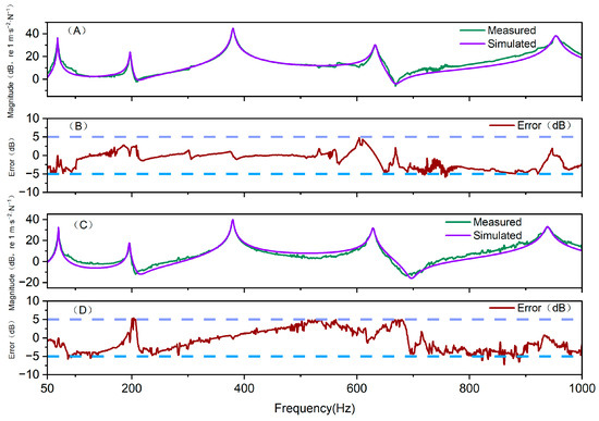
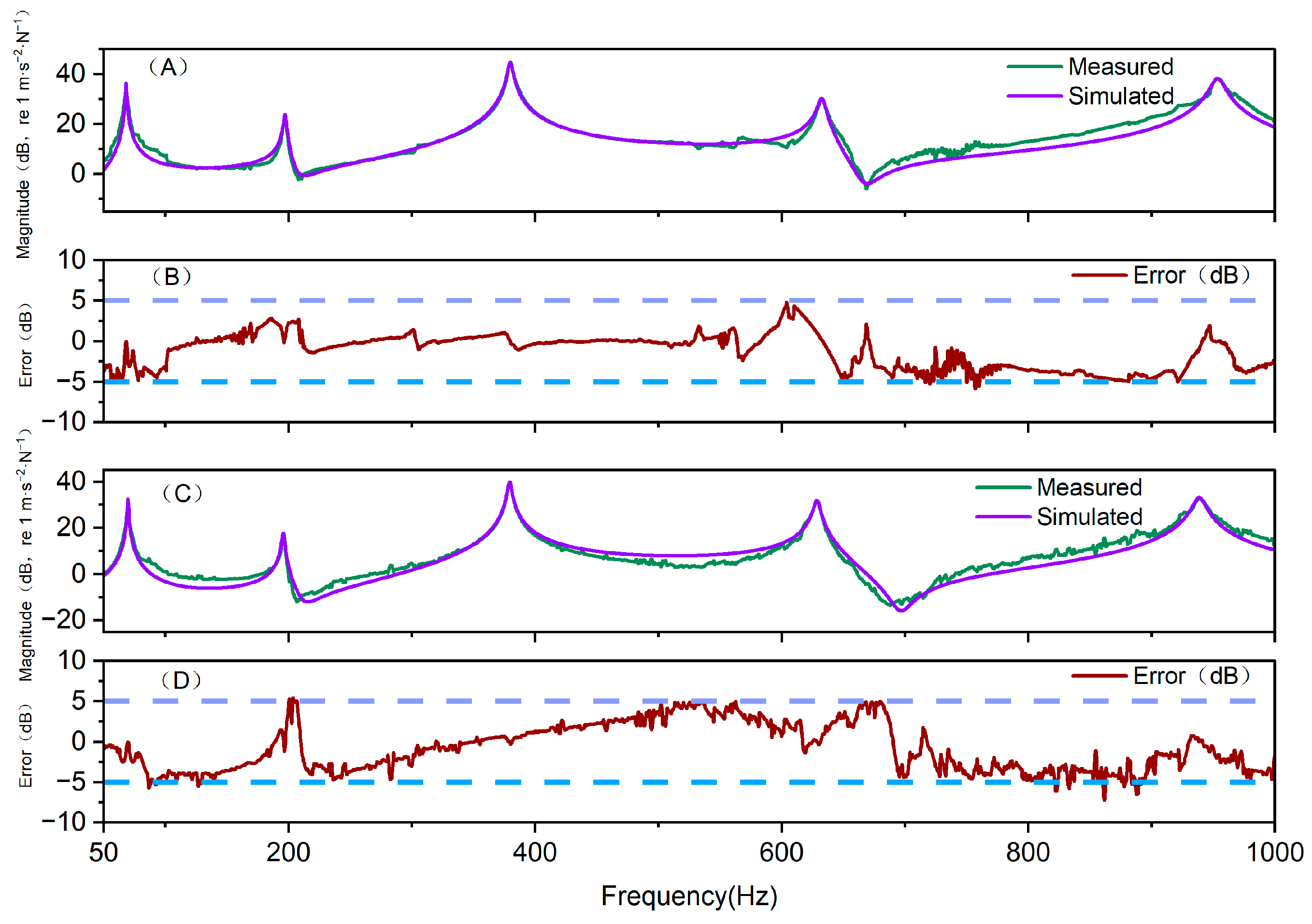
Figure 10 shows the stable reconstruction of the dominant modal responses of specimens (b) and (c). For both specimens, the simulated and measured frequencies of the 1st- to 5th-order main resonance peaks were in good agreement, indicating that the model has good transferability between in resonance-frequency identification. For specimen (b), good fitting was observed near the first, third, and fifth resonance peaks. The error curve generally fluctuates around the zero line, with most frequency points falling within the ±5 dB range. The deviations were mainly concentrated in the valley and local peak–valley transition regions. Specimen (c) is similar to specimen (b), and the position of the main peaks has also been well reconstructed. However, the fluctuations between peaks in the high-frequency range were more complex, and the error was continuously offset in some bands.

Figure 10. Simulated and measured magnitudes and errors for specimens (b) and (c): (A) Simulated and measured magnitudes for specimen (b); (B) magnitude error for specimen (b); (C) simulated and measured magnitudes for specimen (c); (D) magnitude error for specimen (c).

For specimen (b), the RMSE, MAE, and ME within the 50–1000 Hz range were 2.47 dB, 1.85 dB, and −1.24 dB, respectively. For specimen (c), the corresponding values were 3.04 dB, 2.69 dB, and −0.85 dB. In both cases, the model slightly underestimated the magnitude. Based on the ±5 dB error band, the frequency points for specimens (b) and (c) fall within the range of 99.58% and 97.47%, respectively, indicating that the model has good stability for both specimens. The mean absolute errors of specimens (b) and (c) at the five resonance points were 0.14 dB and 0.06 dB, respectively, which are better than the average of the full-band average level. The model can not only accurately characterize the main modal frequencies, but also reliably reproduce the resonance-peak magnitudes.

Table 6 shows the simulated and measured phases and their errors at the poles of specimens (b) and (c). The model has good tracking ability for the phase transitions at the resonance points of both specimens. The phase errors at the first to fifth poles of specimen (b) were 0.62°, 3.50°, 0.49°, 4.34°, and 0.06°, respectively. The deviations at the second and fourth poles were relatively larger but remained within 5°. The corresponding phase errors of specimen (c) were 0.22°, 2.42°, 0.58°, 1.81°, and 0.11°, respectively, all within ±5°. After using the resonance magnitude, damping ratio, and pole phase to jointly calculate the modal residual, the model can not only reproduce the main peak characteristics in magnitude, but also retain the direction and degree of phase transition near the poles. The model effectively represents the magnitude–phase coupling relationship dominated by poles, which is also an important foundation for achieving reusability between different specimens.

Table 6. Simulated and measured phases at the poles of specimens (b) and (c), and their errors.

	Frequency (Hz)	Measured Phase (Deg)	Simulated Phase (Deg)	Error (Deg)
Specimen (b)
1st pole	68.0	−86.74	−87.37	0.62
2nd pole	197.0	+109.45	+112.96	3.50
3rd pole	379.5	+84.74	+84.25	0.49
4th pole	632.5	−76.33	−72.00	4.34
5th pole	953.5	−82.06	−82.00	0.06
Specimen (c)
1st pole	69.5	−85.26	−85.48	0.22
2nd pole	195.5	+103.78	+106.20	2.42
3rd pole	379.0	88.71	+88.13	0.58
4th pole	628.5	−81.21	−79.40	1.81
5th pole	938.5	−83.69	−83.30	0.11

Table 7 shows the measured and simulated anti-resonance frequencies and notch depths of specimens (b) and (c) in the 50–1000 Hz range. The frequency errors of the four anti-resonance points of specimen (b) were −5.0 Hz, −5.0 Hz, −5.0 Hz, and −1.0 Hz, respectively, while the notch-depth errors were +0.21 dB, +1.21 dB, +1.79 dB, and +1.99 dB, respectively. The prediction error of the zero position is relatively small, and the model slightly underestimates the notch depths. The frequency errors of the anti-resonance points of specimen (c) were −2.5 Hz, −9.0 Hz, −0.5 Hz, and −9.0 Hz, respectively, and the notch-depth errors were −3.97 dB, −0.17 dB, +4.87 dB, and −2.28 dB, respectively. The pole identification of the model remained stable for specimen (c), but its reconstruction of the valleys between adjacent peaks was weaker than that of specimen (b). In particular, the depths of local anti-resonance and the position of the valley bottom were more easily affected between specimens. As shown in Figure 10B,D, the main errors were not concentrated at the resonance peaks, but were more distributed in the transition regions between adjacent modes.

Table 7. Comparison of measured and simulated anti-resonance frequencies and notch depths of specimens (b) and (c) in the 50–1000 Hz range.

Zero	Pole Interval	${\mathit{f}}_{\mathit{z},\mathbf{e}\mathbf{x}\mathbf{p}} \left(\mathbf{H}\mathbf{z}\right)$	${\mathit{f}}_{\mathit{z},\mathbf{m}\mathbf{o}\mathbf{d}} \left(\mathbf{H}\mathbf{z}\right)$	$∆{\mathit{f}}_{\mathit{z}} \left(\mathbf{H}\mathbf{z}\right)$	${\mathit{d}}_{\mathit{e}\mathit{x}\mathit{p}} \left(\mathbf{d}\mathbf{B}\right)$	${\mathit{d}}_{\mathit{m}\mathit{o}\mathit{d}} \left(\mathbf{d}\mathbf{B}\right)$	$∆\mathit{d} \left(\mathbf{d}\mathbf{B}\right)$
$Z_b$1	68.0–197.0	125.0	130.0	−5.0	27.89	27.68	+0.21
$Z_b$2	197.0–379.5	208.0	213.0	−5.0	36.31	35.10	+1.21
$Z_b$3	379.5–632.5	532.5	537.5	−5.0	27.32	25.53	+1.79
$Z_b$4	632.5–953.5	668.5	669.5	−1.0	40.10	38.11	+1.99
$Z_c$1	69.5–195.5	133.0	135.5	−2.5	27.35	31.32	−3.97
$Z_c$2	195.5–379.0	206.5	215.5	−9.0	40.70	40.87	−0.17
$Z_c$3	379.0–628.5	513.0	513.5	−0.5	32.91	28.04	+4.87
$Z_c$4	628.5–938.5	688.0	697.0	−9.0	46.10	48.38	−2.28

The model could reconstruct the frequency, magnitude, and phase characteristics of the first-to-fifth main resonance peaks with good accuracy. The errors observed in the anti-resonance intervals mainly come from the reconstruction of inter-peak coupling, anti-resonance depth, and higher-order tail contributions, rather than from failure in pole identification.

4. Conclusions

This study focused on the frequency-domain modal characteristics of wooden beam specimens, aiming to evaluate the reconstruction and parameterization ability of the proposed transfer-function model under controlled testing conditions. A parameterized transfer-function model was established based on the measured frequency response functions, achieving a model representation from experimental measurement to analysis reconstruction. The main conclusions of the study are as follows:

• The experiment utilized Sitka spruce beam specimens, which were tested in the frequency range of 50–1000 Hz under small-magnitude vibration and controlled-moisture-content conditions using non-contact magnetic swept-sine excitation, dual-channel laser Doppler vibrometry, and FFT analysis methods. Based on modal superposition, an analytical transfer-function model was established, and the model was validated through using Bode magnitude–phase plots, Nyquist plots, and time-domain reconstruction.
• Based on the measurement of complex FRFs, a 1st–5th-order transfer-function model was established in the range of 0–1000 Hz. The model can reproduce the measured Bode magnitude and phase responses, with magnitude residuals within ±5 dB, resonance-peak magnitude errors of 0.03–0.73 dB, and pole wrapped-phase deviations of 0.20–5.08°. These results indicate that under small-magnitude and controlled testing conditions, the response of beam specimens can be approximately described as a linear time-invariant system.
• The Nyquist trajectory of the model was continuous and smooth, and all identified poles were located in the left half-plane, confirming the stability and numerical self-consistency of the model. The pole parameters, anti-resonance features, and phase variations of the model can provide a unified description of the dominant resonance and anti-resonance behavior.
• The proposed transfer-function model converted discrete experimental FRF data into continuous and computable modal-parameter representation. Under the current controlled testing conditions, the model provides a physically interpretable basis for evaluating and reconstructing the frequency-domain vibration responses of wooden beam specimens. The model can present the main modal characteristics of the specimens and provide a low-dimensional parameter form.

References

- Bucur, V. The Acoustics of Wood; CRC Press: Boca Raton, FL, USA, 2017. [Google Scholar]
- Bucur, V. A Review on Acoustics of Wood as a Tool for Quality Assessment. Forests 2023, 14, 1545. [Google Scholar] [CrossRef] [Scilit]
- Shi, J.; Yin, S.; Huang, W. Application of vibrational methods in wood performance testing: A short review. BioResources 2025, 20, 4861–4876. [Google Scholar] [CrossRef] [Scilit]
- Viala, R.; Placet, V.; Cogan, S. Simultaneous non-destructive identification of multiple elastic and damping properties of spruce tonewood to improve grading. J. Cult. Herit. 2020, 42, 108–116. [Google Scholar] [CrossRef] [Scilit]
- Quintavalla, M.; Gabrielli, F.; Canevari, C. Grading materials for stringed instruments soundboards: An approach considering the orthotropic elastic and damping properties. Appl. Acoust. 2022, 187, 108521. [Google Scholar] [CrossRef] [Scilit]
- Ducceschi, M.; Duran, S.; Tahvanainen, H.; Ausiello, L. A method to estimate the rectangular orthotropic plate elastic constants using least-squares and Chladni patterns. Appl. Acoust. 2024, 220, 109949. [Google Scholar] [CrossRef] [Scilit]
- Ray, T.; Kaljun, J.; Straže, A. Comparison of the Vibration Damping of the Wood Species Used for the Body of an Electric Guitar on the Vibration Response of Open-Strings. Materials 2021, 14, 5281. [Google Scholar] [CrossRef] [Scilit]
- Glass, S.; Zelinka, S. Moisture Relations and Physical Properties of Wood. In Wood Handbook—Wood as An Engineering Material; Chapter 4 in FPL-GTR-282; U.S. Department of Agriculture, Forest Service, Forest Products Laboratory: Madison, WI, USA, 2021; pp. 4-1–4-22. [Google Scholar]
- Fathi, H.; Nasir, V.; Kazemirad, S. Prediction of the mechanical properties of wood using guided wave propagation and machine learning. Constr. Build. Mater. 2020, 262, 120848. [Google Scholar] [CrossRef] [Scilit]
- Kouroussis, G.; Fekih, L.B.; Descamps, T. Assessment of timber element mechanical properties using experimental modal analysis. Constr. Build. Mater. 2017, 134, 254–261. [Google Scholar] [CrossRef] [Scilit]
- Reynders, E. System identification methods for (operational) modal analysis: Review and comparison. Arch. Comput. Methods Eng. 2012, 19, 51–124. [Google Scholar] [CrossRef] [Scilit]
- Kawrza, M.; Furtmüller, T.; Adam, C.; Maderebner, R. Parameter identification for a point-supported cross laminated timber slab based on experimental and numerical modal analysis. Eur. J. Wood Wood Prod. 2021, 79, 317–333. [Google Scholar] [CrossRef] [Scilit]
- Ao, W.K.; Pavic, A.; Kurent, B.; Perez, F. Novel FRF-based fast modal testing of multi-storey CLT building in operation using wirelessly synchronised data loggers. J. Sound Vib. 2023, 548, 117551. [Google Scholar] [CrossRef] [Scilit]
- Santoni, A.; Bonfiglio, P.; Fausti, P.; Marescotti, C.; Mazzanti, V.; Pompoli, F. Characterization and vibro-acoustic modeling of wood composite panels. Materials 2020, 13, 1897. [Google Scholar] [CrossRef] [Scilit] [PubMed]
- Zhang, L.; He, L.; Liang, Y.; Zhang, J.; Zhang, H.; Zhou, J.; Cui, H.; Li, M.; Miao, Y.; Liu, Z. Modulating the Acoustic Vibration Performance of Wood by Introducing a Periodic Annular Groove Structure. Forests 2023, 14, 2360. [Google Scholar] [CrossRef] [Scilit]
- Deng, L.; Chen, X.; Chen, F.; Liu, X.E.; Jiang, Z. Effect of Environmental Humidity on the Acoustic Vibration Characteristics of Bamboo. Forests 2022, 13, 329. [Google Scholar] [CrossRef] [Scilit]
- Kohantorabi, M.; Ali Hossein, M.; Shahverdi, M.; Roohnia, M. Vibration Based NDT Methods to Verify Wood Drying Efficiency. Drv. Ind. 2015, 66, 221–228. [Google Scholar] [CrossRef] [Scilit]
- Ahmed, S.A.; Adamopoulos, S. Acoustic properties of modified wood under different humid conditions and their relevance for musical instruments. Appl. Acoust. 2018, 140, 92–99. [Google Scholar] [CrossRef] [Scilit]
- Guan, C.; Zhang, H.; Zhou, L.; Wang, X. Dynamic determination of modulus of elasticity of full-size wood composite panels using a vibration method. Constr. Build. Mater. 2015, 100, 201–206. [Google Scholar] [CrossRef] [Scilit]
- Nop, P.; Tippner, J. Influence of dimensions of wooden samples for determination of acoustic parameters and sound timbre. Appl. Acoust. 2022, 196, 108895. [Google Scholar] [CrossRef] [Scilit]
- Bediz, B.; Korkmaz, E.; Ozdoganlar, O.B. An impact excitation system for repeatable, high-bandwidth modal testing of miniature structures. J. Sound Vib. 2014, 333, 2743–2761. [Google Scholar] [CrossRef] [Scilit]
- Merhar, M. Identification of damping of spruce wood (Picea abies) under various levels of moisture content using time-scale decomposition. Polymers 2024, 16, 1313. [Google Scholar] [CrossRef] [Scilit] [PubMed]
- Lämmlein, S.L.; Mannes, D.; Van Damme, B.; Schwarze, F.W.; Burgert, I. The influence of multi-layered varnishes on moisture protection and vibrational properties of violin wood. Sci. Rep. 2019, 9, 18611. [Google Scholar] [CrossRef] [Scilit] [PubMed]
- Inácio, O.; Antunes, J.; Wright, M. Computational modelling of string–body interaction for the violin family and simulation of wolf notes. J. Sound Vib. 2008, 310, 260–286. [Google Scholar] [CrossRef] [Scilit]
- Li, Y.; Dieussaert, E.; Baets, R. Miniaturization of Laser Doppler Vibrometers—A Review. Sensors 2022, 22, 4735. [Google Scholar] [CrossRef] [Scilit]
- Reina, S.; Arcos, R.; Clot, A.; Romeu, J. An Efficient Experimental Methodology for the Assessment of the Dynamic Behaviour of Resilient Elements. Materials 2020, 13, 2889. [Google Scholar] [CrossRef] [Scilit] [PubMed]
- ASTM E1876-15; Standard Test Method for Dynamic Young’s Modulus, Shear Modulus, and Poisson’s Ratio by Impulse Excitation of Vibration. ASTM International: West Conshohocken, PA, USA, 2015.
- Arjunan, A.; Babu, A. Estimation of natural frequency for nonlinear mechanical retention of printed circuit board. Sci. Rep. 2025, 15, 18441. [Google Scholar] [CrossRef] [Scilit]
- Stanbridge, A.; Ewins, D. Modal testing using a scanning laser Doppler vibrometer. Mech. Syst. Signal Process. 1999, 13, 255–270. [Google Scholar] [CrossRef] [Scilit]
- Inman, D.J.; Singh, R.C. Engineering Vibration; Prentice Hall: Englewood Cliffs, NJ, USA, 1994; Volume 3. [Google Scholar]
- Sharma, J.K. Theoretical and experimental modal analysis of beam. In Engineering Vibration, Communication and Information Processing: ICoEVCI 2018, India; Springer: Berlin/Heidelberg, Germany, 2019. [Google Scholar]
- Ewins, D.J. Modal Testing: Theory, Practice and Application; John Wiley & Sons: Hoboken, NJ, USA, 2009. [Google Scholar]
- Avitabile, P. Experimental modal analysis. Sound Vib. 2001, 35, 20–31. [Google Scholar]
- Qu, C.; Tu, G.; Gao, F.; Sun, L.; Pan, S.; Chen, D. Review of bridge structure damping model and identification method. Sustainability 2024, 16, 9410. [Google Scholar] [CrossRef] [Scilit]
- Craig, R.R., Jr.; Kurdila, A.J. Fundamentals of Structural Dynamics; John Wiley & Sons: Hoboken, NJ, USA, 2006. [Google Scholar]
- Matsubara, M.; Saito, A.; Kawamura, S. Estimation of modal parameters by using the ratios of imaginary to real parts of frequency response functions. Arch. Appl. Mech. 2021, 91, 1179–1191. [Google Scholar] [CrossRef] [Scilit]
- ISO 7626-2:2015; Mechanical Vibration and Shock—Experimental Determination of Mechanical Mobility—Part 2: Measurements Using Single-Point Translation Excitation with an Attached Vibration Exciter. International Organization for Standardization: Geneva, Switzerland, 2015.
- Rao, S.S. Vibration of Continuous Systems; John Wiley & Sons: Hoboken, NJ, USA, 2019. [Google Scholar]
- Khasawneh, F.A.; Segalman, D. Exact and numerically stable expressions for Euler-Bernoulli and Timoshenko beam modes. Appl. Acoust. 2019, 151, 215–228. [Google Scholar] [CrossRef] [Scilit]
- Luo, J.; Zhu, S.; Zhai, W. Exact closed-form solution for free vibration of Euler-Bernoulli and Timoshenko beams with intermediate elastic supports. Int. J. Mech. Sci. 2022, 213, 106842. [Google Scholar] [CrossRef] [Scilit]
- Thomson, W. Theory of Vibration with Applications; CRC Press: Boca Raton, FL, USA, 2018. [Google Scholar]
Disclaimer/Publisher’s Note: The statements, opinions and data contained in all publications are solely those of the individual author(s) and contributor(s) and not of MDPI and/or the editor(s). MDPI and/or the editor(s) disclaim responsibility for any injury to people or property resulting from any ideas, methods, instructions or products referred to in the content. |
© 2026 by the authors. Licensee MDPI, Basel, Switzerland. This article is an open access article distributed under the terms and conditions of the Creative Commons Attribution (CC BY) license.