Integrating Pigeon-Inspired Optimization and Support Vector Machines for Forest Aboveground Biomass Estimation

Abstract

Estimating forest aboveground biomass (AGB) in mountainous forest ecosystems remains a significant challenge due to complex terrain, the high cost and limited applicability of traditional field-based methods. To address this issue, a remote sensing-based AGB estimation framework integrating intelligent optimization and machine learning was developed for Mount Tai in eastern China. Sentinel-2 multispectral data were selected to derive 105 candidate variables, including spectral bands, vegetation indices, texture features, and topographic factors, from which 17 key variables were selected using Pearson correlation analysis for model construction. A Support Vector Machine (SVM) optimized by the Pigeon-inspired optimization (PIO) algorithm was developed to adaptively determine optimal hyperparameters, and its performance was compared with that of Random Forest (RF) and standard SVM models. Among the three models, PIO-SVM produced the highest numerical accuracy. For the training dataset, it obtained an R² of 0.85 and an RMSE of 46.12 t/hm². For the testing dataset, it achieved an R² of 0.73 and an RMSE of 62.19 t/hm², compared with 0.72 and 66.25 t/hm² for the standard SVM model and 0.70 and 65.19 t/hm² for the RF model. The spatial distribution of AGB derived from the optimal model shows higher AGB values in the central and northern regions characterized by dense forest cover, in close agreement with field observations. Overall, the results suggest that PIO-based parameter optimization can improve SVM performance for AGB estimation in mountainous forests. This study provides a reliable and efficient framework for regional-scale monitoring of forest biomass and carbon sink dynamics.

1. Introduction

Forest ecosystems constitute a fundamental component of the global terrestrial carbon cycle and play an indispensable role in maintaining ecological security, regulating climate, and enhancing carbon sequestration. As an important indicator of carbon storage and ecosystem processes, AGB is widely used to assess carbon sink capacity and to characterize carbon cycling dynamics [1]. Accurate characterization of the spatial distribution of AGB is therefore essential for providing scientific support for carbon peaking and carbon neutrality strategies, as well as for guiding sustainable regional ecosystem management [2,3].

Conventional AGB estimation methods primarily rely on field plot surveys combined with allometric growth equations. Although these approaches may achieve high accuracy at local scales, they are constrained by substantial labor and financial costs, ecological disturbance, and limited spatial representativeness. Consequently, the large-scale and efficient utilization of them, particularly in complex mountainous areas, still presents challenges [4,5]. As remote sensing technology has continued to develop, non-destructive AGB estimation methods that integrate multi-source satellite imagery with ground-based observations have emerged as a dominant research paradigm [6,7]. However, the relationships between remote sensing variables and forest structural parameters are often highly nonlinear and scale-dependent, which limits the ability of traditional linear regression models to capture these complex interactions [8]. In this context, machine learning approaches, such as random forests and support vector machines, have emerged as key techniques for forest biomass estimation from remote sensing data due to their strong capability to model high-dimensional and nonlinear relationships.

Machine learning models have been widely applied in forest aboveground biomass estimation. For example, Foody et al. compared multiple linear regression and backpropagation (BP) neural networks for tropical forest biomass estimation using Landsat TM data [9]. Zhang et al. applied remote sensing variables derived from Landsat and MODIS time-series data to biomass estimation and reported satisfactory model performance [10]. Dang et al. proposed a robust forest biomass estimation model using Sentinel-2 imagery by extracting a diverse set of feature variables [11]. Similarly, Wai et al. estimated aboveground biomass for two forest types in Myanmar by combining Sentinel-2 data with machine-learning and geostatistical algorithms, further demonstrating the applicability of optical satellite imagery for biomass mapping in heterogeneous forest environments [12]. In China, Wang Yifu et al. [13] and Lin Zhuo et al. [14] developed biomass estimation models for specific tree species using BP neural networks and SVMs, respectively, while Zhang Pengchao et al. employed MODIS data in combination with a random forest model for estimating forest AGB across the Qinghai–Tibet Plateau [15]. Collectively, these studies demonstrate the effectiveness of machine learning approaches for forest biomass estimation; they further show that differences in model performance are closely related to forest type, terrain complexity, and variable selection. To address the reliance of traditional machine learning models on manual expertise for hyperparameter tuning and to further improve model generalization and stability in complex environments, this study introduces and applies a swarm intelligence-based optimization method, namely the PIO algorithm. The PIO algorithm simulates pigeons’ homing behavior through geomagnetic navigation and landmark recognition, thereby achieving a balance between global exploration and local exploitation. As a result, it demonstrates advantages such as fast convergence and strong global optimization capability [16]. Previous studies suggest that integrating the PIO algorithm with machine learning models, particularly SVMs, can improve prediction accuracy and robustness; however, its systematic application to forest AGB estimation using remote sensing data in complex mountainous regions, as well as comprehensive comparisons with mainstream models, remains limited.

Mount Tai, a representative temperate forest ecosystem in eastern China, provides an ideal study area for remote sensing-based estimation of forest parameters in complex terrain due to its pronounced topographic variability and diverse vegetation, which is dominated primarily by pine–oak forests. Focusing on the Mount Tai region in Shandong Province, this study integrates Sentinel-2 multispectral imagery with ground-based plot survey data to develop and systematically compare the performance of RF, SVM and PIO-SVM models for AGB estimation. The contribution of this study lies not in the development of a fundamentally new optimization algorithm, but in the integration of a PIO-based hyperparameter optimization strategy with the SVM model for forest AGB estimation in a complex mountainous environment. Thus, the novelty of this study is reflected in a workflow-level technical contribution and its application to Mount Tai, where the performance of the PIO-SVM framework is systematically evaluated against RF and conventional SVM under the same data and feature conditions. This comparison provides an empirical basis for assessing the applicability of optimized machine-learning models for mountainous forest AGB estimation and offers practical support for regional biomass monitoring and carbon stock assessment.

2. Materials and Methods

2.1. Overview of the Study Area

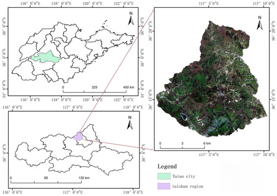
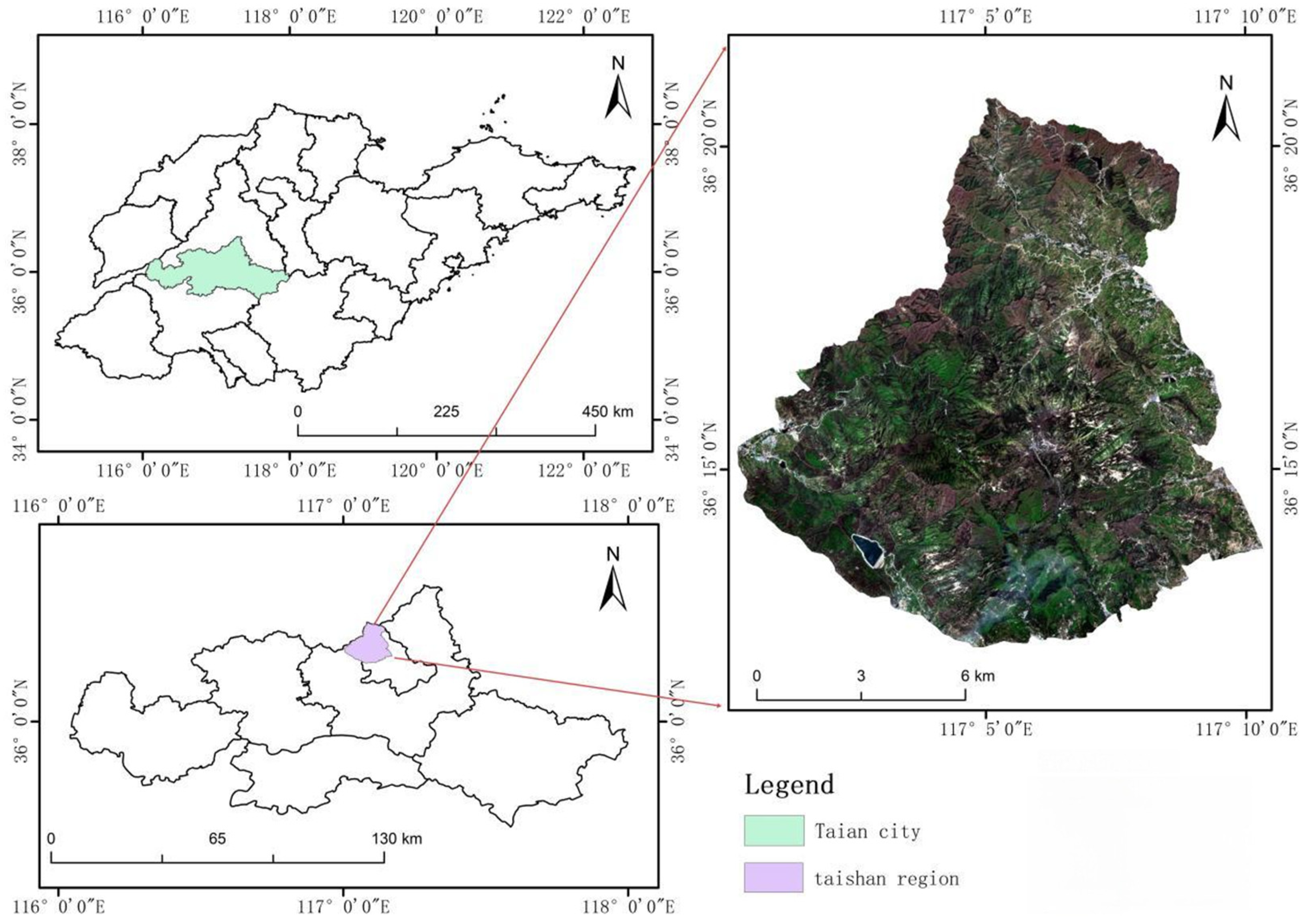
The study area is situated in Taian City, Shandong Province, China, encompassing the Mount Tai region (116°50′–117°12′ E, 36°11′–36°31′ N). Located at the boundary between Jinan and Taian, the area covers approximately 426 km² and includes the highest peak on the North China Plain. The climate of the study area is warm temperate continental monsoonal, with an average annual temperature of 12.6 °C and annual precipitation of around 758 mm over the long term, most of which occurs between June and September. The terrain is characterized by steep mountainous landscapes, with elevation gradually decreasing from northwest to southeast. Jade Emperor Peak, the highest summit in the study area, stands at 1545 m above sea level, while mountainous terrain covers over 90% of the region. Forests cover approximately 80% of the region, and the dominant vegetation types include deciduous broadleaf forests (e.g., oak species), coniferous forests (e.g., Pinus tabulaeformis and Platycladus orientalis), and mixed forests [17]. In addition, portions of the study area fall within the protection zone of a World Cultural and Natural Heritage site. The location of the study area is shown in Figure 1.

Figure 1. Location of the study area.

2.2. Remote Sensing Data

The Sentinel-2 remote sensing imagery used in this study was acquired from the European Space Agency (ESA, Paris, France) Copernicus Data Centre on 27 June 2024. Sentinel-2A scenes with cloud cover of less than 5% were selected to minimize atmospheric interference. Image pre-processing, including atmospheric correction, resampling, and spatial subsetting, was carried out using SNAP 9.0 and ENVI 5.3 software to generate surface reflectance products. Sentinel-2 is a core component of the ESA Copernicus programme. The mission was originally based on Sentinel-2A and Sentinel-2B, and Sentinel-2C was launched in 2024 to support the continuity of high-resolution multispectral observations. In this study, Sentinel-2A imagery was used. Sentinel-2 carries a Multispectral Instrument (MSI) that provides 13 spectral bands distributed across the visible, VNIR, and SWIR regions, with original spatial resolutions of 10 m, 20 m, and 60 m. To ensure spatial consistency among variables, all Sentinel-2 bands used in this study were resampled to 10 m spatial resolution before feature extraction and model construction. The DEM-derived terrain variables were also aligned to the same spatial grid, so that spectral, vegetation-index, texture, and topographic variables shared a consistent spatial resolution and extent before plot-level extraction and subsequent modeling.

2.3. Ground Survey Data

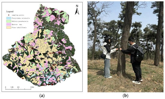
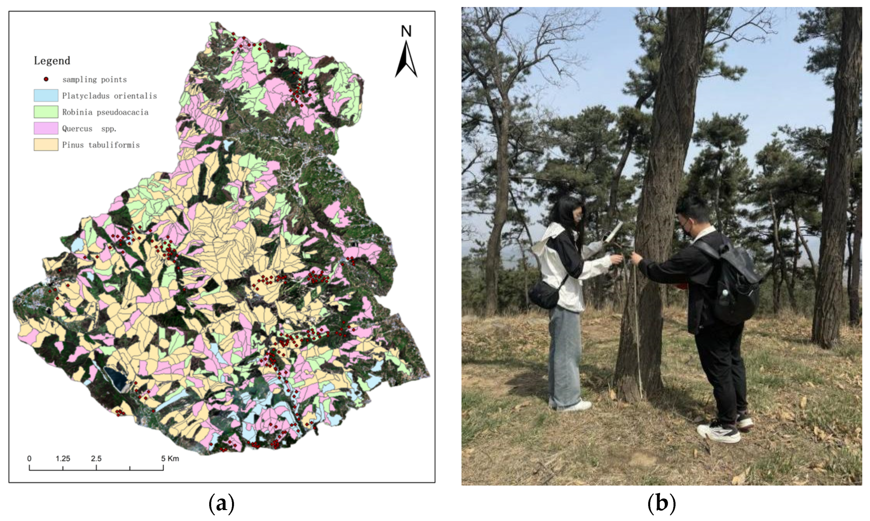
Field data were collected between May and June 2024. The dominant tree species—including Quercus spp., Robinia pseudoacacia, Pinus tabuliformis, and Platycladus orientalis—were identified through field investigations combined with existing forestry inventory data. Following the principles of species representativeness, uniform spatial distribution, and measurement feasibility, representative sample plots with a size of 10 m × 10 m were established for each species. The geographic coordinates and elevation of the center of each plot were recorded using a GPS receiver, and detailed stand attributes within each plot were measured. In total, 205 sample plots were surveyed across the four target species (Pinus tabuliformis, Platycladus orientalis, Robinia pseudoacacia, and Quercus spp.). The collected field data included diameter at breast height (DBH), root collar diameter (RCD), tree height (H), and crown width (CW). Due to constraints such as steep mountainous terrain and forest fire prevention regulations, the sample plots could not be uniformly distributed across the entire study area. Figure 2 presents the spatial arrangement of the sample plots.

Figure 2. (a) Distribution of sample sites by species; (b) Field data collection.

The allometric equations applied for aboveground biomass calculation in this study were chosen according to the Guidelines on Carbon Accounting and Monitoring for Afforestation Projects issued by the National Forestry and Grassland Administration of China. Specifically, for Platycladus orientalis and Pinus tabuliformis, province-specific equations for Shandong were adopted. For Robinia pseudoacacia, because no Shandong-specific equation was available in the guideline, the equation for Hebei Province was used. For Quercus spp., because no Shandong-specific equation was available, the equation for Beijing was used. Regional AGB was calculated based on field sampling data collected within the study area, the mean values appeared in Table 1 and the specific equations employed are listed in Table 2. In these equations, diameter at breast height (DBH, denoted as D in equations) is expressed in centimeters (cm), tree height is measured in meters (m), and biomass is reported in metric tons per hectare (t/hm²). For tree species lacking region-specific allometric equations, biomass estimates were obtained using equations developed for ecologically similar neighboring regions.

Table 1. Summary of Field Survey Data.

Tree Species	Number	Minimum (t/hm2)	Maximum (t/hm2)	Mean AGB (t/hm2)	Standard Deviation (t/hm2)	Coefficient of Variation (%)
Platycladus orientalis	45	70.4047	519.5040	260.6584	123.9561	47.5550
Quercus spp.	47	50.1650	541.6702	202.2876	127.4144	62.9867
Pinus tabuliformis	53	45.9000	567.1940	241.6070	133.9167	55.4275
Robinia pseudoacacia	60	43.0483	460.9291	222.9042	109.0712	48.9319

Note: Number refers to the number of sample plots for each species rather than the number of individual trees.

Table 2. Allometric Growth Model of Major Tree Species in the Study Area.

Tree Species	Allometric Growth Equation	References
Platycladus orientalis	1.034885 + 0.0223(D2H) + 0.095(D2H)0.571 + 0.714(D2H)0.583	[18]
Quercus spp.	0.0369(D2H)0.9165 + 0.00051(D2H)1.3377 + 0.00021(D2H)1.171	[18]
Pinus tabuliformis	0.946835 + 0.214(D2H) + 0.77(D2H)0.679 + 0.848(D2H)0.594	[18]
Robinia pseudoacacia	0.05527(D2H)0.8576 + 0.02425(D2H)0.7908 + 0.0545(D2H)0.4574	[18]

Note: D represents diameter at breast height (cm), and H represents tree height (m).

2.4. Methodological Flowchart

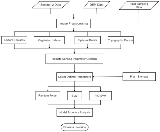
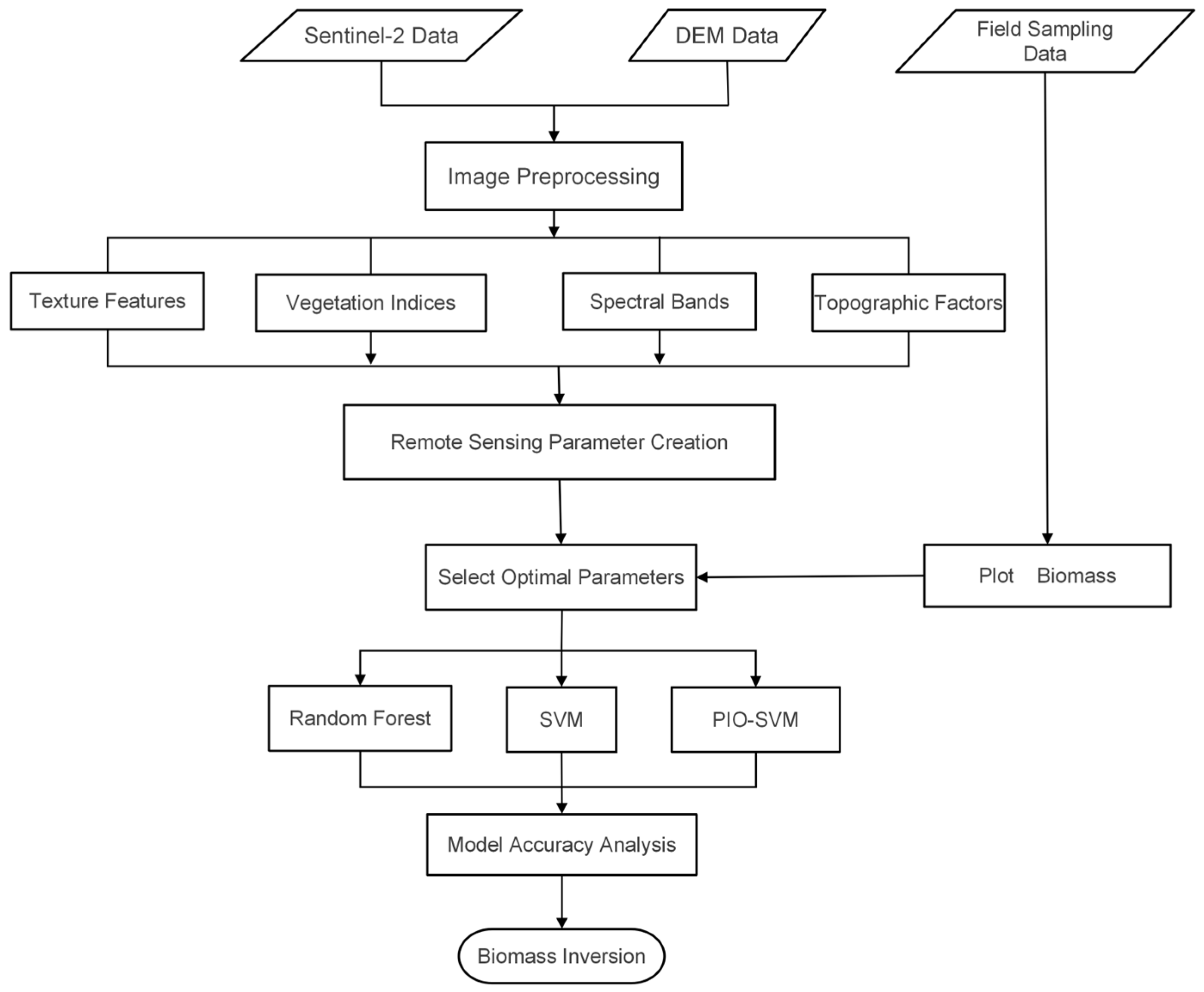
In this study, ArcGIS 10.8 software was used to extract a broad range of remote sensing variables associated with forest aboveground biomass as the first step of the overall workflow, followed by their integration with AGB estimates derived from field sampling data. After performing correlation analysis and feature selection, multiple machine learning models are developed and evaluated in terms of estimation accuracy. Through this workflow, a spatially explicit map of forest AGB was generated for the entire study area, as illustrated in Figure 3.

Figure 3. Method flow chart.

2.5. Feature Variable Extraction and Selection

In forest AGB estimation studies, spectral variables and vegetation indices are widely used as important predictors because they can effectively reflect vegetation condition, canopy cover, and biomass-related variation [19]. In this study, Sentinel-2 multispectral imagery was utilized, including Bands 2 (blue), 3 (green), 4 (red), 5–7 (red-edge), 8 (near-infrared), and 11–12 (shortwave infrared). Based on these spectral bands, six widely used vegetation indices were derived: the Normalized Difference Vegetation Index (NDVI), Fractional Vegetation Cover (FVC), Enhanced Vegetation Index (EVI), Normalized Difference Red Edge Index (NDRE), Optimized Soil-Adjusted Vegetation Index (OSAVI), and Kernel Normalized Difference Vegetation Index (KNDVI).

Texture features were additionally incorporated to characterize the spatial structure and heterogeneity of forest vegetation, thereby improving AGB estimation accuracy [20]. To reduce information redundancy and extract representative texture information, texture metrics were derived from the selected 10-band imagery, namely mean, variance, homogeneity, contrast, dissimilarity, entropy, correlation and second moment. Window size selection is critical in texture analysis: overly small windows are prone to noise, whereas excessively large windows may obscure spatial heterogeneity. Accordingly, texture information was generated using the Gray-Level Co-occurrence Matrix (GLCM) method with a moving window of 3 × 3 pixels, which provides a balance between detail preservation and feature representativeness [21]. Principal Component Analysis (PCA) was subsequently applied to reduce feature dimensionality while retaining at least 90% of the total variance.

In addition, the Tasseled Cap Transformation provided three components—brightness, greenness, and wetness—which were integrated with topographic variables to form the feature set used for AGB estimation [22]. Terrain-related variables were generated from a 30 m Digital Elevation Model (DEM) obtained from the Geospatial Data Cloud platform, including slope, aspect, terrain wetness index (TWI), and terrain solar radiation index. The incorporation of these variables improves the model’s ability to account for complex terrain effects and ecological variability. The feature variables used in this study are summarized in Table 3.

Table 3. Feature variables used in this study.

Variables	Feature Variable	Formula	References
Spectral Variable	Band reflectance (Sentinel-2 bands)	Band i (i = 2,3, …, 12)	[23]
	Normalized difference vegetation index (NDVI)	(NIR − R)/(NIR + R)	[24]
	Enhanced vegetation index (EVI)	2.5 × (NIR − R)/(NIR + 6R − 7.5B + 1)	[25]
	Fractional Vegetation Cover (FVC)	(NDVI − NDVI_min)/(NDVI_max − NDVI_min)	[26]
	Normalized Difference Red Edge Index (NDRE)	(NIR − RE)/(NIR + RE)	[27]
	Optimized Soil Adjusted Vegetation Index (OSAVI)	(1 + 0.16)(NIR − R)/(NIR + R + 0.16)	[28]
	Kernel Normalized Difference Vegetation Index (KNDVI)	tanh (NDVI2)	[29]
Texture feature	Mean	${\sum }_{\mathrm{i},\mathrm{j}=0}^{\mathrm{N}-1}{\mathrm{i}\mathrm{p}}_{\mathrm{i}\mathrm{j}}$	[21]
	Contrast	${\sum }_{\mathrm{i},\mathrm{j}=0}^{\mathrm{N}-1}{{\mathrm{i}\mathrm{p}}_{\mathrm{i}\mathrm{j}}\left(\mathrm{i}-\mathrm{j}\right)}^2$	[21]
	Variance	${\sum }_{\mathrm{i},\mathrm{j}=0}^{\mathrm{N}-1}{{\mathrm{p}}_{\mathrm{i}\mathrm{j}}\left(\mathrm{i}=\mathrm{M}\mathrm{E}\right)}^2$	[21]
	Dissimilarity	${\sum }_{\mathrm{i},\mathrm{j}=0}^{\mathrm{N}-1}{\mathrm{i}\mathrm{p}}_{\mathrm{i}\mathrm{j}}\left|\mathrm{i}-\mathrm{j}\right|$	[21]
	Homogeneity	${\sum }_{\mathrm{i},\mathrm{j}=0}^{\mathrm{N}-1}\mathrm{i}{\displaystyle \frac{{\mathrm{p}}_{\mathrm{i}\mathrm{j}}}{1+{\left(\mathrm{i}-\mathrm{j}\right)}^2}}$	[21]
	Entropy	${\sum }_{\mathrm{i},\mathrm{j}=0}^{\mathrm{N}-1}{\mathrm{i}\mathrm{p}}_{\mathrm{i}\mathrm{j}}\left(-\ln {\mathrm{P}}_{\mathrm{i}\mathrm{j}}\right)$	[21]
	Correlation	${\sum }_{\mathrm{i},\mathrm{j}=0}^{\mathrm{N}-1}\mathrm{i}\mathrm{P}\mathrm{i}\mathrm{j}\left[{\displaystyle \frac{\left(\mathrm{i}-\mathrm{M}\mathrm{E}\right)\left(\mathrm{j}-\mathrm{M}\mathrm{E}\right)}{\sqrt{{\mathrm{V}\mathrm{A}}_{\mathrm{i}}{\mathrm{V}\mathrm{A}}_{\mathrm{i}}}}}\right]$	[21]
	Second moment	${\sum }_{\mathrm{i},\mathrm{j}=0}^{\mathrm{N}-1}{\mathrm{i}\mathrm{p}}_{\mathrm{i}\mathrm{j}}^2$	[21]
Tasseled Cap Transformation	Brightness	0.3510B + 0.3813G + 0.3437R + 0.7196NIR + 0.2396SWIR1 + 0.1949SWIR2	[30]
	Greenness	−0.3599B − 0.3533G − 0.4734R + 0.6633NIR + 0.0087SWIR1 − 0.2856SWIR2	[30]
	Wetness	0.2578B + 0.2305G + 0.0883R + 0.1071NIR − 0.7611SWIR1 − 0.5308SWIR2	[30]

Notes: B, G, and R denote the blue, green, and red bands, respectively; NIR denotes the near-infrared band; RE denotes the red-edge band; ME, mean; VAi, variance; SWIR1 and SWIR2 represent shortwave infrared bands 1 and 2, respectively.

2.6. Pearson Correlation

Before constructing the estimation models, Pearson correlation analysis was performed to identify feature variables that are significantly associated with forest AGB, thereby reducing feature redundancy and mitigating the risk of model overfitting. This analysis is used to quantify the strength of linear relationships between candidate independent variables and AGB. The Pearson correlation coefficient r is defined as:

$$r={\displaystyle \frac{\sum _{i=1}^n \left(x_i-\overline{x}\right)\left(y_i-\overline{y}\right)}{\sqrt{\sum _{i=1}^n (x_i-\overline{x}{)}^2(y_i-\overline{y}{)}^2}}}$$

(1)

where n is the sample size; x_i and y_i represent the observed values of variables x and y at sample point i, respectively; and $\overline{x}$ and $\overline{y}$ are the average values of variables x and y. The correlation coefficient r ranges from −1 to 1, with its absolute value indicating the strength of linear association between the variables. In this study, Pearson correlation analysis was used as a preliminary feature-screening step. Variables were retained when they showed a statistically significant correlation with AGB at the 0.05 level (p < 0.05) and an absolute Pearson correlation coefficient greater than 0.60 (|r| > 0.60). This procedure was used to reduce the dimensionality of the candidate feature set before subsequent machine-learning modeling. Because several retained variables were derived from related spectral bands, vegetation indices, and texture measures, some intercorrelation may still remain among them. Therefore, multicollinearity was noted but was not used as the sole exclusion criterion at this stage.

2.7. Random Forest Algorithm

Random Forest (RF) is an ensemble learning method that extends traditional decision tree approaches by combining multiple decision trees within a unified framework [31]. Based on bagging, RF introduces additional randomness during tree construction by resampling both training samples and feature subsets from the original dataset, which increases model diversity and helps reduce overfitting [32]. The predictions from individual trees are then aggregated, typically by averaging in regression tasks, to generate the final output. Owing to this structure, RF has strong capability for modeling nonlinear relationships, while also providing useful measures of variable importance. Because of its robustness, generalization ability, and relative ease of implementation, RF has been widely used in classification, regression, and feature selection studies, including forest parameter estimation [33,34]. Previous studies have also demonstrated the theoretical consistency and reliability of RF [35]. In this study, RF was used as one of the comparison models for forest AGB estimation.

2.8. Support Vector Machine Algorithm

Support Vector Machine (SVM) is a supervised learning algorithm derived from statistical learning theory and structural risk minimization [36]. The method aims to determine an appropriate separating boundary in the feature space while maintaining a large margin between the boundary and nearby samples. For nonlinear problems, SVM uses kernel functions to transform the original variables into another feature space, where complex relationships can be modeled more effectively. Owing to its strong generalization capability, SVM has clear advantages in tasks involving small sample datasets and high-dimensional variables [36]. In this study, the regression form of SVM, namely Support Vector Regression (SVR), was adopted to model forest AGB as a continuous variable.

2.9. Pigeon-Inspired Optimization Algorithm

Pigeon-inspired optimization is a novel swarm intelligence-based optimization algorithm characterized by a simple operational mechanism and a limited number of control parameters. Compared with other swarm intelligence algorithms, PIO is relatively easy to implement and exhibits fast convergence behavior [16]. The algorithm was first proposed in 2014 by Duan Haibin et al., inspired by the collective homing behavior of pigeons [37]. Since its introduction, PIO and its variants have demonstrated strong performance in a range of complex optimization tasks, including parameter optimization, scheduling problems, and machine learning model tuning.

The PIO algorithm models pigeon homing behavior through two main components: the map-and-compass operator and the landmark operator. When pigeons are far from their destination, they rely on geomagnetic fields and the sun to determine flight direction; this behavior is simulated by the map-and-compass operator [16]. As pigeons approach their destination, they increasingly depend on familiar landmarks for navigation, which is represented by the landmark operator. Accordingly, the map-and-compass operator is constructed based on geomagnetic and solar navigation principles, whereas the landmark operator is based on landmark-based guidance.

Pigeons are assumed to possess innate magnetic sensitivity, enabling them to perceive geomagnetic fields and adjust their flight direction according to the position of the sun during long-distance homing. As the flock approaches its destination, the influence of geomagnetic cues and solar navigation gradually diminishes. In the PIO framework, the solution space is defined as a D-dimensional space, where the position and velocity of the i-th pigeon (i = 1, 2, …, N) represent candidate solutions. At each iteration, the positions and velocities of all pigeons are updated according to predefined update rules, as expressed in Equations (2) and (3):

$$V_{i\left(t\right)}= V_{i\left(t-1\right)}\cdot e^{\left\{-R \cdot t\right\}}+ \left\{rand\right\}\cdot \left(X_g- X_{i\left(t-1\right)}\right)$$

(2)

$$X_{i\left(t\right)}=X_{i\left(t-1\right)}+V_{i\left(t\right)}$$

(3)

where R denotes the map-and-compass factor (0 < R < 1), X represents the global best position, t is the current iteration number, where rand is a random variable following a uniform distribution over the range [0, 1].

The landmark operator is established based on pigeons’ navigation behavior when approaching their destination, where landmark guidance becomes more dominant than geomagnetic navigation. If pigeons are unfamiliar with the landmarks at their current location, they fly under the guidance of nearby pigeons. Once a landmark or familiar location is identified, pigeons rely on accumulated experience to guide their flight independently. In the landmark model, $N_{\mathrm{p}}\left(t\right)$ denotes the number of pigeons in the t-th generation, and $X_{c\left(t\right)}$ represents the center position of the pigeon swarm. Assuming that each pigeon can fly directly toward the destination, the population size is updated as:

$$N_{\mathrm{p}}\left(t\right) = ceil\left[N_{\mathrm{p}}\right(t-1) /2]$$

(4)

The center position of the pigeon swarm is calculated as a fitness-weighted mean:

$$X_{c\left(t\right)}=[\sum (X_{\mathrm{i}}\left(t\right)\times \mathrm{f}\mathrm{i}\mathrm{t}\mathrm{n}\mathrm{e}\mathrm{s}\mathrm{s}\left(X_{\mathrm{i}}\right(t\left)\right)\left)\right]÷ [N_{\mathrm{p}}\times \sum \mathrm{f}\mathrm{i}\mathrm{t}\mathrm{n}\mathrm{e}\mathrm{s}\mathrm{s}(X_{\mathrm{i}}\left(t\right)\left)\right]$$

(5)

Subsequently, the position of each pigeon is updated according to:

$$X_{i\left(t\right)}= X_{i\left(t-1\right)}+\left\{rand\right\}\cdot \left(X_{c\left(t\right)}- X_{i\left(t-1\right)}\right)$$

(6)

where fitness(X) denotes the fitness value of each pigeon and indicates the quality of the corresponding solution.

In this study, PIO was applied to optimize the key SVM hyperparameters, including the penalty parameter C and the insensitive loss parameter ε. By automatically searching for optimal parameter combinations, the PIO-SVM framework aims to enhance the accuracy and robustness of forest AGB estimation models [38].

Model accuracy assessment relies on appropriate evaluation metrics that effectively reflect both model fitting ability and predictive performance. In this study, three machine learning models were employed to estimate forest aboveground biomass in the Taishan forest region: PIO-SVM, SVM, and RF model. To quantitatively evaluate and compare the performance of these regression models, two widely used statistical metrics were used: the root mean square error (RMSE) and the coefficient of determination (R²).

The dataset was randomly partitioned into a training subset and a testing subset using a 7:3 ratio. The evaluation metrics were calculated as follows:

$$R^2=1-{\displaystyle \frac{\sum _{i=1}^n(y_i-{\widehat{y}}_i{)}^2}{\sum _{i=1}^n(y_i-\overline{y}{)}^2}}$$

(7)

$$RMSE=\sqrt{{\displaystyle \frac{1}{n}}\sum _{i=1}^n(y_i-{\widehat{y}}_i{)}^2}$$

(8)

where n denotes the number of samples, y_i represents the observed AGB value, ${\widehat{y}}_i$ is the model-predicted AGB value, and $\overline{y}$ is the mean of the observed AGB values. RMSE reflects the overall prediction error magnitude, while R² indicates the proportion of variance in AGB explained by the model.

3. Results

3.1. Correlation Analysis

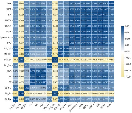
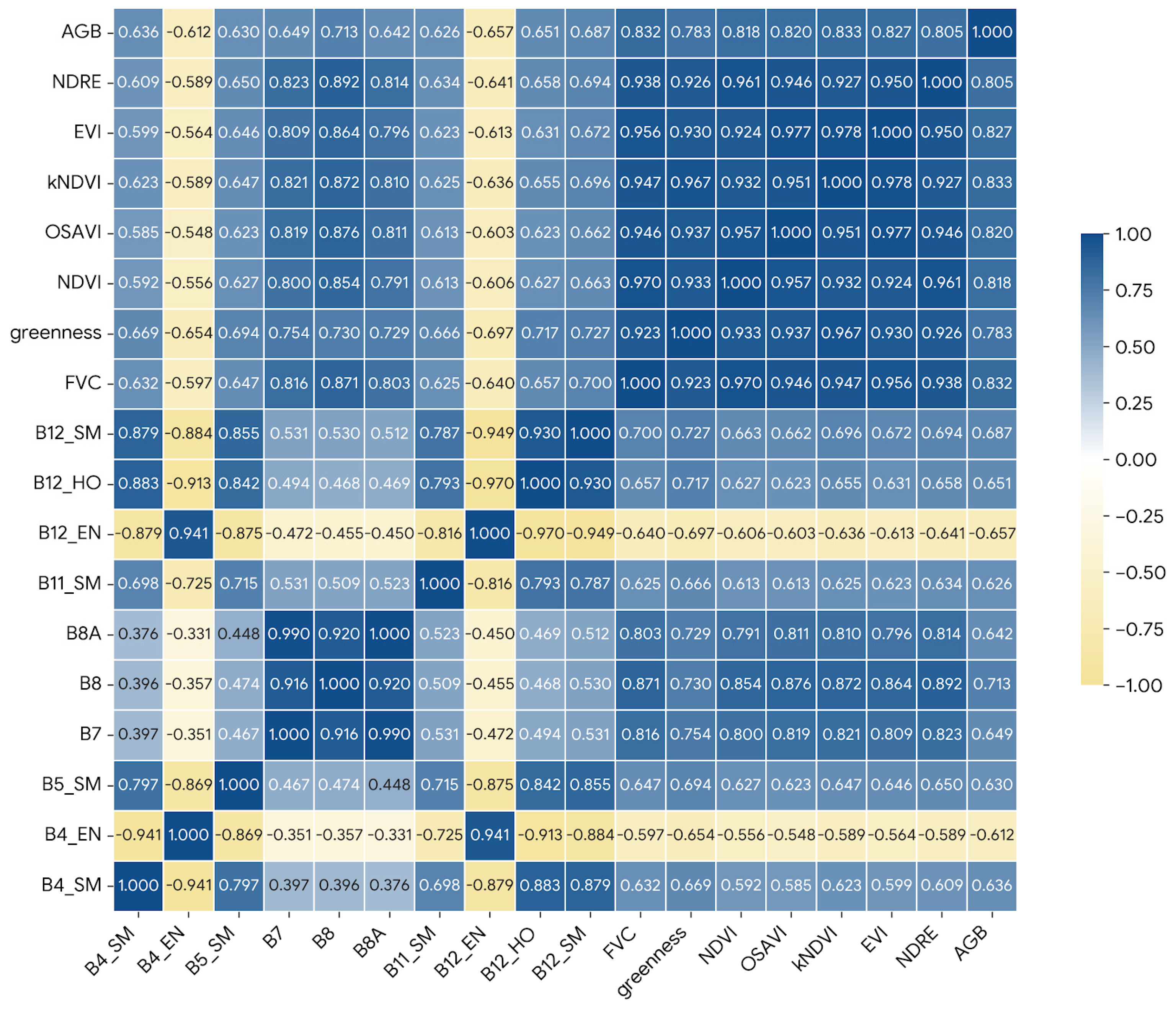
After extracting a total of 105 remote-sensing-derived feature variables, including 10 spectral bands, 6 vegetation indices, 80 texture features, 6 environmental factors, and 3 Tasseled Cap Transformations, Pearson correlation analysis was used to identify feature variables that exhibited significant correlations with forest AGB. Variables with p < 0.05 and |r| > 0.60 were retained. Based on these criteria, 17 variables were selected for subsequent machine-learning modeling, namely B4_SM, B4_EN, B5_SM, B8, B8A, B11_SM, B12_EN, B12_SM, B12_HO, B7, NDRE, OSAVI, EVI, FVC, greenness, NDVI, and KNDVI. Among these variables, KNDVI showed the strongest correlation with AGB, as summarized in Figure 4 and Table 4. Because some retained variables were derived from related spectral and vegetation information, a certain degree of intercorrelation may still exist among them. However, the purpose of this step was to reduce the number of candidate predictors before model construction rather than to eliminate all redundancy among predictors.

Figure 4. Correlation coefficient matrix between characteristic variables and AGB.

Table 4. Significant Correlation Coefficients for Remote Sensing Parameters.

Variable	Correlation Coefficient
B4_SM	0.636 ***
B4_EN	−0.612 ***
B5_SM	0.630 ***
B8	0.713 ***
B8A	0.642 ***
B11_SM	0.626 ***
B12_EN	−0.657 ***
B12_SM	−0.687 ***
B12_HO	0.651 ***
B7	0.649 ***
NDRE	0.805 ***
OSAVI	0.820 ***
EVI	0.827 ***
FVC	0.832 ***
greenness	0.783 ***
NDVI	0.818 ***
KNDVI	0.833 ***

Note: *** denotes significance at the 1% level.

3.2. Evaluation of Model Accuracy

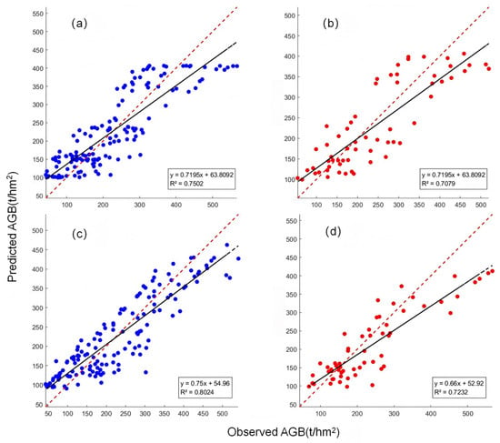
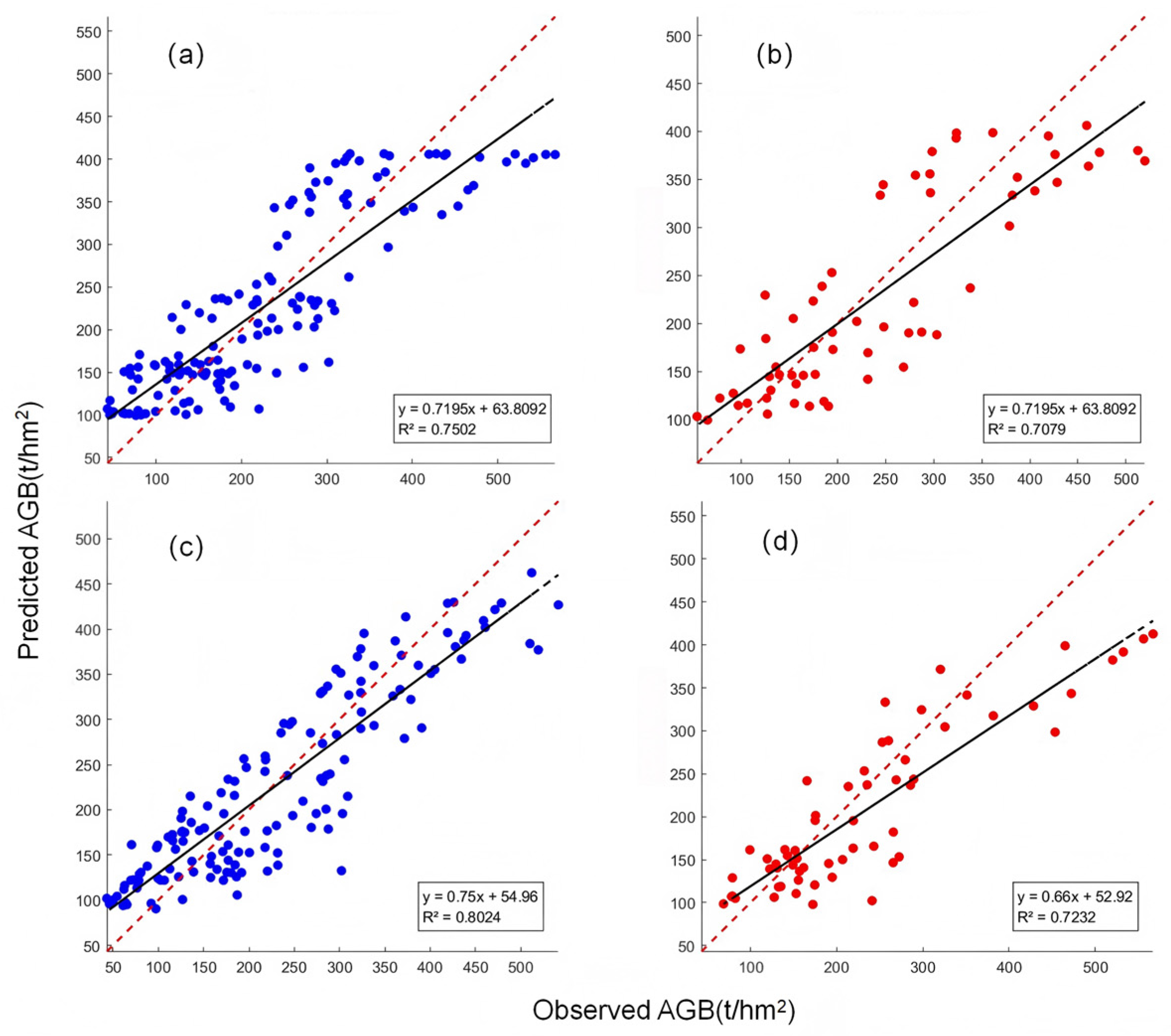
The selected model parameters and measured aboveground biomass data from 205 sample plots were imported into the MATLAB R2021a environment for model training and evaluation. A random split was performed to divide the dataset into training and testing sets in a proportion of 7:3. The conventional RF model was implemented using the TreeBagger function in regression mode. The number of trees was set to 500, the minimum leaf size was set to 20, and OOB prediction and OOB-based predictor importance were enabled. The remaining parameters were kept at the MATLAB default settings. The conventional SVM model was implemented using support vector regression with an RBF kernel. After preliminary trial-and-error testing, the BoxConstraint parameter was fixed at 0.3 and the insensitive loss parameter ε was fixed at 0.1 as baseline settings. Input and output variables were normalized before model training. Scatter plots illustrating the relationships between measured and predicted AGB values for the different models are presented in Figure 5.

Figure 5. Scatter plot between predicted and observed AGB. (a) Modeling Set of RF; (b) Validation set of RF; (c) Modeling Set of SVM; (d) Validation set of SVM. The dashed line represents the 1:1 reference line between observed and predicted AGB values.

In addition to the single 7:3 train-test split, five-fold cross-validation was further conducted for the RF, SVM, and PIO-SVM models to reduce the influence of a single random partition and to evaluate model robustness. In each round, four folds were used for training and the remaining fold was used for validation. This process was repeated five times, and the mean and standard deviation of R² and RMSE were calculated across the five folds.

3.3. AGB Estimation Based on PIO-SVM

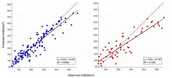
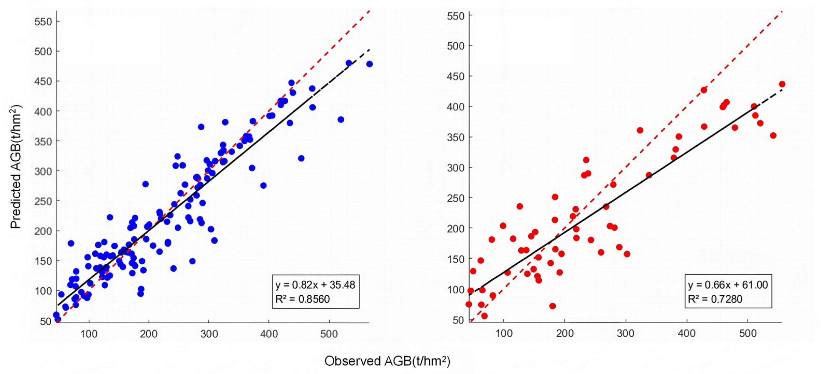
Forest aboveground biomass estimation was conducted using SVM optimized by the PIO algorithm. For the PIO-SVM model, the pigeon-inspired optimization algorithm was used to optimize the penalty parameter (C) and the insensitive loss parameter (ε) of the SVM model, while the RBF kernel was retained and KernelScale was kept at MATLAB’s automatic setting. The population size was set to 20, the maximum number of iterations was set to 30, and the map-and-compass factor was set to 0.2. The search ranges of C and ε were 0.1–100 and 0.001–1, respectively. During the optimization process, the fitness of each candidate parameter combination was evaluated using the mean RMSE from five-fold cross-validation on the training dataset. The optimization process was terminated when the maximum number of iterations was reached. The optimal parameter combination obtained in this study was C = 2.8933 and ε = 0.09514. The estimation results obtained using the PIO-SVM model are presented in Figure 6.

Figure 6. Scatter plots of the predicted AGB by PIO-SVM model. The dashed line represents the 1:1 reference line between observed and predicted AGB values.

3.4. Model Accuracy Evaluation

In this study, three machine learning algorithms—RF, SVM, and PIO-SVM—were employed to construct forest aboveground biomass estimation models for the Mount Tai region. All models were developed using Sentinel-2 multispectral imagery in combination with an optimized set of environmental variables. The quantitative accuracy assessment results for the three models are summarized in Table 5.

Table 5. Accuracy Evaluation Results for Different Models.

Model	Modeling Set		Validation Set
	R2	RMSE (t/hm2)	R2	RMSE (t/hm2)
RF	0.75	62.41	0.70	65.19
SVM	0.80	54.85	0.72	66.25
PIO-SVM	0.85	46.12	0.73	62.19

As reported in Table 5, the three models all achieved reasonable performance for forest AGB estimation, with validation R² values ranging from 0.70 to 0.73. On the training dataset, the PIO-SVM model showed the highest R² (0.85) and the lowest RMSE (46.12 t/hm²). On the validation dataset, it yielded an R² of 0.73 and an RMSE of 62.19 t/hm², compared with 0.72 and 66.25 t/hm² for the conventional SVM model and 0.70 and 65.19 t/hm² for the RF model. These results indicate that the PIO-SVM model provided the best numerical performance among the three models under the present random split, although the improvement over the conventional SVM model on the validation dataset was relatively limited.

To reduce the dependence on a single random split, five-fold cross-validation was further conducted for the three models, and the results are presented in Table 6. Under cross-validation, PIO-SVM achieved the best overall predictive performance, with the highest mean R² (0.661) and the lowest mean RMSE (68.41 t/hm²). In comparison, RF produced a mean R² of 0.647 and a mean RMSE of 69.36 t/hm², whereas the conventional SVM showed the lowest predictive accuracy, with a mean R² of 0.615 and a mean RMSE of 73.74 t/hm². In addition, PIO-SVM exhibited the smallest standard deviations for both R² and RMSE, indicating improved model stability after parameter optimization. Overall, the cross-validation results further support the effectiveness of the PIO-based optimization strategy for improving SVM performance in forest AGB estimation.

Table 6. Five-fold cross-validation results of RF, SVM, and PIO-SVM models.

Model	CV R2 (Mean ± Std)	CV RMSE (t/hm2) (Mean ± Std)
RF	0.647 ± 0.057	69.36 ± 4.13
SVM	0.615 ± 0.106	73.74 ± 5.42
PIO-SVM	0.661 ± 0.042	68.41 ± 4.06

3.5. Forest Aboveground Biomass Estimation Mapping

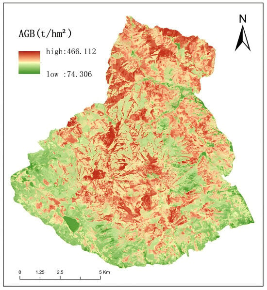
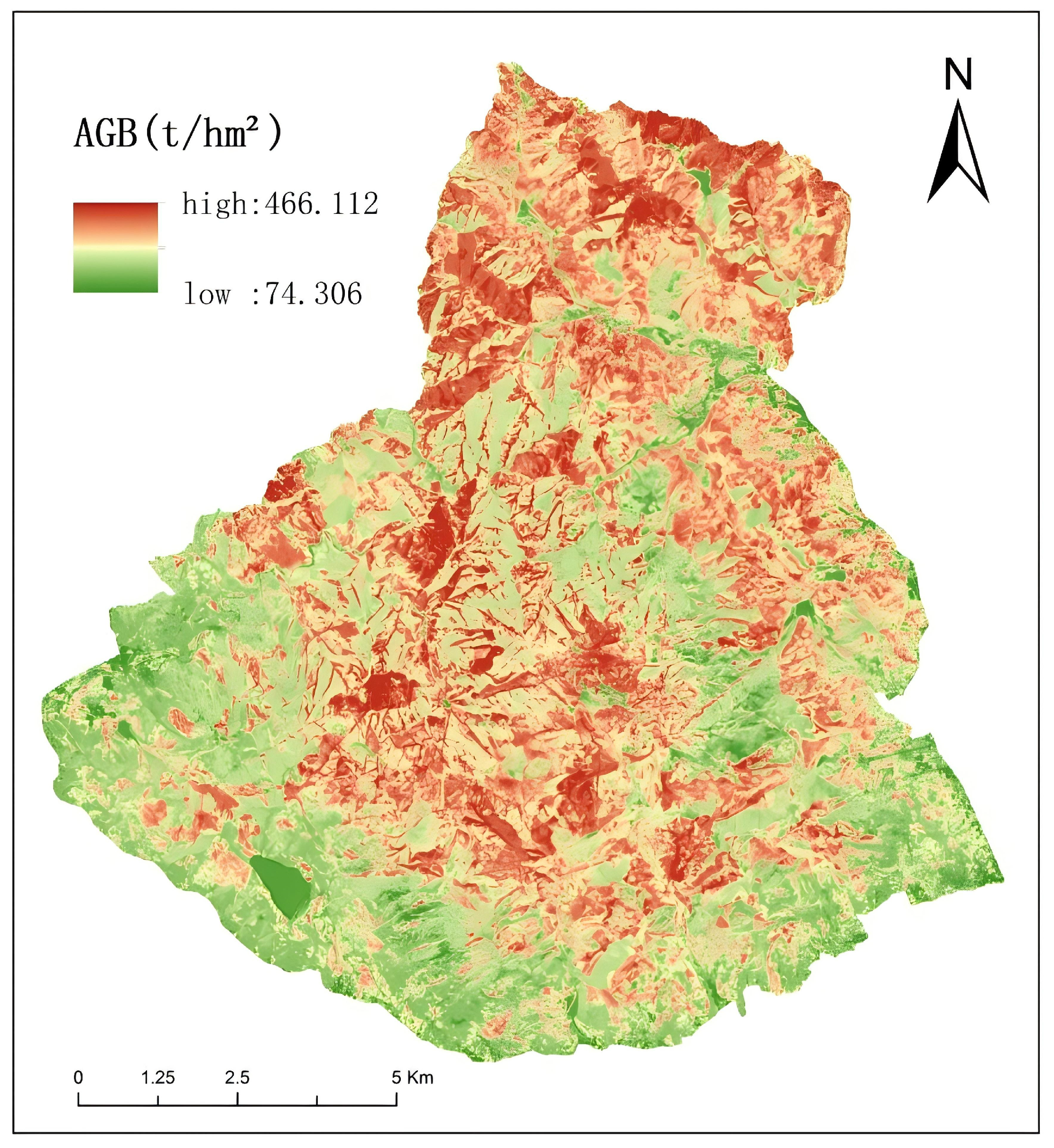
After model optimization, the selected PIO-SVM model was employed to predict forest aboveground biomass for the whole study area. The findings show that forest AGB is mainly distributed in the central and northern parts of the study area, where forest cover is relatively dense. Biomass density exhibits a clear spatial gradient, gradually increasing from the peripheral areas toward the interior of the region. This spatial pattern is highly consistent with field survey observations, demonstrating the reliability of the PIO-SVM model for large-scale forest AGB mapping. The mapped distribution of estimated AGB across the study area is displayed in Figure 7.

Figure 7. Spatial distribution of forest AGB estimated using the PIO-SVM model in the study area.

4. Discussion

4.1. Performance Comparison of Different Machine Learning Models

Machine learning models differ in their ability to handle complex data structures and environmental heterogeneity. In the mountainous forest environment of Mount Tai, the three models examined in this study—RF, SVM, and PIO-SVM—all produced acceptable AGB estimation results. Among them, the PIO-SVM model achieved the best numerical performance, especially on the training dataset, and showed slightly better validation results than the RF and conventional SVM models. However, the improvement over the conventional SVM model on the validation dataset was relatively limited.

To reduce the influence of a single random partition, five-fold cross-validation was further conducted. The cross-validation results showed that PIO-SVM still achieved the best overall predictive performance, with the highest mean R² and the lowest mean RMSE among the three models. In addition, PIO-SVM exhibited the smallest standard deviations for both R² and RMSE, indicating improved model stability after parameter optimization. These results suggest that the superiority of PIO-SVM was not solely dependent on a single train-test split, but was also supported by repeated cross-validation.

The slightly better performance of the PIO-SVM model may be related to the global optimization capability of the PIO algorithm in tuning key SVM hyperparameters, including the penalty coefficient C and the insensitive loss parameter ε. Conventional SVM models are highly sensitive to hyperparameter selection, and suboptimal configurations may result in convergence to local optima or reduced generalization performance. By contrast, RF models reduce variance through ensemble learning and exhibit strong robustness to noise with minimal parameter tuning; however, their ability to capture highly complex nonlinear relationships may be constrained in heterogeneous forest environments. The PIO algorithm employed in this study balances global exploration and local exploitation of the parameter space by simulating the two-stage homing behavior of pigeons, represented by a global map-and-compass operator and a local landmark operator. This optimization strategy enables the SVM to identify parameter combinations closer to the global optimum, thereby improving predictive accuracy, convergence stability, and robustness in modeling complex nonlinear relationships between multi-source remote sensing features and forest AGB in mountainous terrain. Consequently, the PIO-SVM model achieves a favorable balance between accuracy and stability under complex terrain conditions, demonstrating the effectiveness of PIO for enhancing traditional machine learning models.

The dominance of vegetation-index variables such as NDVI, FVC, and NDRE in this study is ecologically meaningful. In mountainous forests, aboveground biomass is closely associated with canopy density, foliage abundance, and photosynthetic activity, all of which strongly influence spectral reflectance. NDVI and FVC mainly reflect canopy cover and greenness conditions and are therefore sensitive to variation in forest growth status and biomass accumulation, especially in areas with relatively continuous vegetation cover. NDRE, which incorporates the red-edge region, is particularly useful in forest environments because it is more sensitive to chlorophyll content and canopy vitality than conventional visible-band indices and is less prone to saturation under moderate-to-high biomass conditions. Therefore, these vegetation indices can capture both canopy development and physiological status, making them effective predictors of AGB in the Mount Tai region.

Terrain and canopy structure also play important roles in shaping model behavior in mountainous forests. Large elevation differences in Mount Tai create strong spatial variability in illumination, temperature, soil moisture, and hydrothermal conditions, which in turn affect forest growth patterns and spectral responses. At the same time, coniferous, broadleaf, and mixed forests differ in crown architecture, canopy closure, leaf traits, and seasonal dynamics, causing the same biomass level to produce different spectral or textural responses under different stand conditions. This partly explains why topographic variables and texture-related variables improved model performance when combined with spectral and vegetation-index variables. It also suggests that model behavior in mountainous forests is jointly controlled by vegetation physiological information, canopy structural heterogeneity, and terrain-related environmental gradients.

4.2. Consistency Analysis and Comparison with Previous Studies

The findings of this study are generally consistent with previous research emphasizing the role of optimization strategies in improving forest AGB estimation accuracy. Existing studies have demonstrated that model performance can be enhanced either by refining feature selection procedures or by improving model parameterization, particularly when high-dimensional remote sensing datasets are involved.

For example, Wang et al. constructed an SVR model based on Lasso-based feature selection, with an emphasis on reducing feature redundancy and improving generalization performance [38]. Although both studies aim to improve model performance, the present study emphasizes parameter-space optimization through adaptive hyperparameter tuning using the PIO algorithm. The results indicate that this strategy effectively improved the predictive performance of SVM. A related conclusion was reported by Chen et al., who evaluated the transferability of spectral variables and prediction models for forest aboveground biomass mapping and showed that model performance can vary markedly across forest conditions and feature sets, highlighting the importance of both model generalization and variable selection [39].

In contrast, Luo et al. employed regression kriging to correct spatially autocorrelated residuals from Random Forest predictions, thereby improving spatial mapping accuracy, particularly by mitigating overestimation and underestimation at extreme values [40]. In the present study, residual-based spatial correction was not conducted. Instead, terrain-related factors were considered at an earlier stage of analysis. Variables such as slope and terrain wetness index were included as candidate factors during feature screening to examine their potential associations with forest growth conditions. The inclusion of these variables contributes to more realistic spatial patterns in the AGB estimates produced by the PIO-SVM model, particularly in areas with pronounced terrain variation. In general, post-processing spatial correction methods and feature-selection strategies and parameter-optimization approaches should be considered complementary rather than mutually exclusive. Integrating the parameter optimization strengths of the PIO-SVM framework with spatial residual correction methods such as regression kriging represents a promising avenue for further enhancing forest AGB estimation accuracy.

4.3. Limitations and Outlook

Although the PIO-SVM model shows relatively good performance in this study, several limitations should be acknowledged, mainly associated with data sources, terrain conditions, and sampling constraints. First, optical remote sensing data are subject to spectral saturation in areas with high biomass. Under dense canopy conditions, the reflectance signals recorded by sensors such as Sentinel-2 tend to saturate in the visible and near-infrared bands, reducing sensitivity to further increases in AGB. As a result, biomass in high-density forest stands may be underestimated, a phenomenon that has also been reported in previous studies. Second, the complex terrain and heterogeneous forest composition of the Mount Tai region introduce additional uncertainty into the modeling process. Large elevation differences lead to spatial variability in illumination and moisture conditions, which in turn affect vegetation growth and spectral responses. In addition, coniferous, broadleaf, and mixed forests exhibit different canopy structures and seasonal characteristics, making it difficult to establish a single relationship that performs equally well across all forest types. Although texture features and topographic variables were examined during feature screening, estimation errors still occur in areas with steep slopes or structurally complex mixed forests. Uncertainty may also arise from the allometric equations used to derive plot-level AGB. In this study, Shandong-specific equations were adopted for Platycladus orientalis and Pinus tabuliformis, whereas the equation for Robinia pseudoacacia was taken from Hebei Province and that for Quercus spp. was taken from Beijing because no corresponding equations for Shandong were available in the national guideline. Although these equations were selected from geographically adjacent regions, their use may still introduce additional uncertainty into plot-level AGB estimation and should be taken into account when interpreting the modeling results. Third, the spatial distribution of field samples imposes limitations on model generalization. Due to accessibility constraints, sample plots were not evenly distributed across the study area, with fewer observations located in high-elevation or steep terrain. In addition, although the sample sizes of the four target tree species were relatively comparable, the distribution of plots among species and environmental gradients was not fully balanced. This may have affected the representation of certain stand conditions and may in turn influence the reliability of AGB estimation at both the stand and regional scales. Furthermore, some forest age classes were underrepresented in the dataset, which may also contribute to uncertainty in model performance. Overall, these limitations indicate that further improvements could be achieved by integrating complementary data sources, such as active remote sensing data, expanding field sampling coverage, and refining modeling strategies for heterogeneous mountainous forests.

To address these limitations, future research should pursue several complementary directions. At the data level, multisource data fusion integrating optical, radar, and LiDAR data offers a promising approach for mitigating spectral saturation effects. Radar data such as Sentinel-1 SAR or ALOS-2 PALSAR-2 are sensitive to vegetation vertical structure, while airborne or satellite LiDAR can directly capture three-dimensional forest structural information, thereby enabling the construction of feature sets with stronger physical interpretability and improved discrimination in high-biomass regions. At the methodological level, further integration of advanced modeling approaches is warranted. Combining PIO algorithms with deep learning architectures (e.g., convolutional neural networks or Transformer-based models) may facilitate the automated extraction of deeper spatial–spectral features. In addition, incorporating spatial statistical techniques—such as coupling PIO-SVM with regression kriging for residual correction—could establish a hybrid framework integrating intelligent parameter optimization with spatial error correction, thereby reducing prediction bias and improving spatial continuity.

Finally, to boost the ecological interpretability and applicability of AGB estimation models, future research ought to further integrate ecological processes by incorporating multidimensional factors such as forest age, species composition, soil properties, climate variability, and human disturbances. This transition from purely data-driven modeling toward a data–mechanism synergistic framework would not only improve estimation accuracy but also support long-term monitoring of forest carbon sinks, ecosystem dynamics, and the scientific assessment of regional carbon neutrality strategies.

In addition, although five-fold cross-validation was introduced in this study to reduce the influence of a single random split, spatial validation was not implemented. Because the sample plots were unevenly distributed across environmental gradients and topographic conditions, spatial autocorrelation may still affect model evaluation to some extent. Therefore, future studies should further assess model robustness using spatial block validation or other spatially explicit validation strategies, so as to improve the reliability of model transferability and regional-scale application in complex mountainous forests.

5. Conclusions

A robust framework for estimating aboveground biomass (AGB) in the Mount Tai region, a temperate mountainous forest area in eastern China, was established by integrating multisource remote sensing data and intelligent parameter optimization. The performance of the proposed PIO-SVM model was evaluated against standard SVM and RF models. The main conclusions can be summarized as follows.

(1)

Feature screening based on Pearson correlation analysis identified spectral, red-edge, vegetation-index, texture, and topographic variables as important contributors to the spatial variability of forest AGB in mountainous environments. Among these, FVC, KNDVI, and NDRE showed strong correlations with field-measured AGB, indicating their usefulness for biomass estimation in complex terrain.

(2)

Among the three tested models, the PIO-SVM model achieved the best numerical performance under the single 7:3 train-test split, with higher training accuracy and slightly better validation results than the conventional SVM and RF models. In addition, the five-fold cross-validation results further showed that PIO-SVM yielded the best overall predictive performance, with the highest mean R², the lowest mean RMSE, and the smallest variability among the three models. These results indicate that PIO-based parameter optimization can improve both the predictive accuracy and stability of SVM for forest AGB estimation in complex mountainous environments.

(3)

The spatial distribution of AGB derived from the PIO-SVM model showed clear spatial heterogeneity across the study area, with relatively higher biomass values concentrated in the central and northern forested regions of Mount Tai. This pattern was generally consistent with field survey observations, indicating that the model can provide useful support for regional-scale biomass mapping in mountainous forest environments.

(4)

Future studies should further improve both model accuracy and ecological interpretability by incorporating additional ecological and stand-related variables, such as species composition, soil properties, climate variability, and stand age. The integration of these factors, together with multisource remote sensing data and improved validation strategies, would help strengthen the applicability of AGB estimation models in heterogeneous mountainous forests.

References

- Xu, W.Y.; Jin, X.B.; Yang, X.H.; Wang, Z.Q.; Liu, J.; Wang, D.; Dan, W.; Zhou, Y.K. Spatial grid-based estimation of forest vegetation biomass in China. J. Nat. Resour. 2018, 33, 1725–1741. [Google Scholar] [CrossRef] [Scilit]
- Kumar, L.; Mutanga, O. Remote sensing of above-ground biomass. Remote Sens. 2017, 9, 935. [Google Scholar] [CrossRef] [Scilit]
- Saatchi, S.S.; Harris, N.L.; Brown, S.; Lefsky, M.; Mitchard, E.T.A.; Salas, W.; Zutta, B.R.; Buermann, W.; Lewis, S.L.; Hagen, S.; et al. Benchmark map of forest carbon stocks in tropical regions across three continents. Proc. Natl. Acad. Sci. USA 2011, 108, 9899–9904. [Google Scholar] [CrossRef] [Scilit]
- Ahmad, A.; Gilani, H.; Ahmad, S.R. Forest Aboveground Biomass Estimation and Mapping through High-Resolution Optical Satellite Imagery—A Literature Review. Forests 2021, 12, 914. [Google Scholar] [CrossRef] [Scilit]
- Breiman, L. Random forests. Mach. Learn. 2001, 45, 5–32. [Google Scholar] [CrossRef] [Scilit]
- Zou, W.T.; Zeng, W.S. Advances in forest biomass and carbon stock estimation. World For. Res. 2025, 38, 32–38. [Google Scholar] [CrossRef]
- Tian, L.; Wu, X.; Tao, Y.; Li, M.; Qian, C.; Liao, L.; Fu, W. Review of remote sensing-based methods for forest aboveground biomass estimation: Progress, challenges, and prospects. Forests 2023, 14, 1086. [Google Scholar] [CrossRef] [Scilit]
- Hengl, T.; Heuvelink, G.B.M.; Rossiter, D.G. About regression-kriging: From equations to case studies. Comput. Geosci. 2007, 33, 1301–1315. [Google Scholar] [CrossRef] [Scilit]
- Foody, G.M.; Boyd, D.S.; Cutler, M.E.J. Predictive relations of tropical forest biomass from Landsat TM data and their transferability between regions. Remote Sens. Environ. 2003, 85, 463–474. [Google Scholar] [CrossRef] [Scilit]
- Zhang, B.H.; Zhang, L.; Xie, D.; Yin, X.; Liu, C.; Liu, G. Application of synthetic NDVI time series blended from Landsat and MODIS data for grassland biomass estimation. Remote Sens. 2015, 8, 10. [Google Scholar] [CrossRef] [Scilit]
- Dang, A.T.N.; Nandy, S.; Srinet, R.; Luong, N.V.; Ghosh, S.; Kumar, A.S. Forest aboveground biomass estimation using machine learning regression algorithm in Yok Don National Park, Vietnam. Ecol. Inform. 2019, 50, 24–32. [Google Scholar] [CrossRef] [Scilit]
- Wai, P.; Su, H.; Li, M. Estimating Aboveground Biomass of Two Different Forest Types in Myanmar from Sentinel-2 Data with Machine Learning and Geostatistical Algorithms. Remote Sens. 2022, 14, 2146. [Google Scholar] [CrossRef] [Scilit]
- Wang, Y.F.; Sun, Y.J.; Guo, X.Y. Standing biomass model of Pinus massoniana based on BP neural network. J. Beijing For. Univ. 2013, 35, 17–21. [Google Scholar] [CrossRef]
- Lin, Z.; Wu, C.Z.; Hong, W.; Hong, T. Harvesting model of artificial cypress forests based on BP neural network and support vector machine. J. Beijing For. Univ. 2015, 37, 42–47. [Google Scholar] [CrossRef]
- Zhang, P.C.; Liang, Y.; Liu, B.; Ma, T.X.; Wu, M.M. Remote sensing estimation of forest above-ground biomass on the Qinghai–Tibet Plateau based on random forest models. J. Ecol. 2023, 42, 415–424. [Google Scholar] [CrossRef]
- Liu, H.; Yan, X.; Wu, Q. An improved pigeon-inspired optimisation algorithm and its application in parameter inversion. Symmetry 2019, 11, 1291. [Google Scholar] [CrossRef] [Scilit]
- Liu, S.T.; Gao, P.; Liu, P.W.; Niu, X.; Wang, B. Assessment of ecosystem services and their value in the Taishan forest ecosystem. Acta Ecol. Sin. 2017, 37, 3302–3310. [Google Scholar] [CrossRef] [Scilit]
- Guidelines on Carbon Accounting and Monitoring for Afforestation Project. Available online: https://std.samr.gov.cn/hb/search/stdHBDetailed?id=8B1827F1BB6BBB19E05397BE0A0AB44A (accessed on 12 August 2024).
- Hao, Q.; Huang, C. Review of forest aboveground biomass estimation based on remote sensing data. Chin. J. Plant Ecol. 2023, 47, 1356–1374. [Google Scholar] [CrossRef] [Scilit]
- Berberoglu, S.; Lloyd, C.D.; Atkinson, P.M.; Curran, P.J. The integration of spectral and textural information using neural networks for land cover mapping in the Mediterranean. Comput. Geosci. 2000, 26, 385–396. [Google Scholar] [CrossRef] [Scilit]
- Haralick, R.M.; Shanmugam, K.; Dinstein, I. Textural features for image classification. IEEE Trans. Syst. Man Cybern. 1973, 3, 610–621. [Google Scholar] [CrossRef] [Scilit]
- Stoyanov, A. Application of Tasseled Cap Transformation of Sentinel-2—MSI Data for Forest Monitoring and Change Detection on Territory of Natural Park “BLUE STONES”. Environ. Sci. Proc. 2022, 22, 42. [Google Scholar] [CrossRef] [Scilit]
- Jiang, F.; Kutia, M.; Ma, K.; Chen, S.; Long, J.; Sun, H. Estimating aboveground biomass of coniferous forest using spectral variables, land surface temperature and soil moisture. Sci. Total Environ. 2021, 785, 147335. [Google Scholar] [CrossRef] [Scilit] [PubMed]
- Tucker, C.J. Red and photographic infrared linear combinations for monitoring vegetation. Remote Sens. Environ. 1979, 8, 127–150. [Google Scholar] [CrossRef] [Scilit]
- Huete, A.; Didan, K.; Miura, T.; Rodriguez, E.P.; Gao, X.; Ferreira, L.G. Overview of the radiometric and biophysical performance of the MODIS vegetation indices. Remote Sens. Environ. 2002, 83, 195–213. [Google Scholar] [CrossRef] [Scilit]
- Purevdorj, T.S.; Tateishi, R.; Ishiyama, T.; Honda, Y. Relationships between percent vegetation cover and vegetation indices. Int. J. Remote Sens. 1998, 19, 3519–3535. [Google Scholar] [CrossRef] [Scilit]
- Sharifi, A.; Felegari, S. Remotely sensed normalized difference red-edge index for rangeland biomass estimation. Aircr. Eng. Aerosp. Technol. 2023, 95, 1128–1136. [Google Scholar] [CrossRef] [Scilit]
- Rondeaux, G.; Steven, M.; Baret, F. Optimization of soil-adjusted vegetation indices. Remote Sens. Environ. 1996, 55, 95–107. [Google Scholar] [CrossRef] [Scilit]
- Guo, B.; Xu, M.; Zhang, R.; Lu, M. Dynamic monitoring of rocky desertification using Sentinel-2 images and KNDVI. Geomat. Nat. Hazards Risk 2024, 15, 2399659. [Google Scholar] [CrossRef] [Scilit]
- Shi, T.; Xu, H. Derivation of tasseled cap transformation coefficients for Sentinel-2 MSI data. IEEE J. Sel. Top. Appl. Earth Obs. Remote Sens. 2019, 12, 4038–4048. [Google Scholar] [CrossRef] [Scilit]
- Cutler, A.; Cutler, D.R.; Stevens, J.R. Random forests. In Ensemble Machine Learning: Methods and Applications; Springer: New York, NY, USA, 2012; pp. 157–175. [Google Scholar] [CrossRef] [Scilit]
- Belgiu, M.; Drăguț, L. Random forest in remote sensing: A review of applications and future directions. ISPRS J. Photogramm. Remote Sens. 2016, 114, 24–31. [Google Scholar] [CrossRef] [Scilit]
- Houghton, R.A.; Butman, D.; Bunn, A.G.; Krankina, O.N.; Schlesinger, P.; A Stone, T. Mapping Russian forest biomass with satellite and inventory data. Environ. Res. Lett. 2007, 2, 045032. [Google Scholar] [CrossRef] [Scilit]
- Xiong, K.; Li, S.F.; Xing, Y.J. Remote sensing estimation of aboveground biomass in forest lands of Yuanling County, Hunan Province. Cent. South For. Surv. Plan. 2024, 43, 44–50. [Google Scholar] [CrossRef]
- Scornet, E.; Biau, G.; Vert, J.-P. Consistency of random forests. Ann. Stat. 2015, 43, 1716–1741. [Google Scholar] [CrossRef] [Scilit]
- Ding, S.F.; Qi, B.J.; Tan, H.Y. Review of support vector machine theory and algorithms. J. Univ. Electron. Sci. Technol. China 2011, 40, 2–10. [Google Scholar] [CrossRef]
- Duan, H.; Qiao, P. Pigeon-inspired optimization: A new swarm intelligence optimizer for air robot path planning. Int. J. Intell. Comput. Cybern. 2014, 7, 24–37. [Google Scholar] [CrossRef] [Scilit]
- Wang, P.; Tan, S.; Zhang, G.; Wang, S.; Wu, X. Remote sensing estimation of forest aboveground biomass based on Lasso-SVR. Forests 2022, 13, 1597. [Google Scholar] [CrossRef] [Scilit]
- Chen, L.; Lin, H.; Long, J.; Liu, Z.; Yang, P.; Zhang, T. Evaluating the Transferability of Spectral Variables and Prediction Models for Mapping Forest Aboveground Biomass Using Transfer Learning Methods. Remote Sens. 2023, 15, 5358. [Google Scholar] [CrossRef] [Scilit]
- Luo, Y.N.; Yan, L.; Zhou, Z.; Huang, D.; Cai, L.; Du, S.; Yang, Y.; Huang, Y.; Li, Q. Estimation of forest aboveground biomass in complex mountainous areas using regression kriging. Forests 2024, 15, 1734. [Google Scholar] [CrossRef] [Scilit]
Disclaimer/Publisher’s Note: The statements, opinions and data contained in all publications are solely those of the individual author(s) and contributor(s) and not of MDPI and/or the editor(s). MDPI and/or the editor(s) disclaim responsibility for any injury to people or property resulting from any ideas, methods, instructions or products referred to in the content. |
© 2026 by the authors. Licensee MDPI, Basel, Switzerland. This article is an open access article distributed under the terms and conditions of the Creative Commons Attribution (CC BY) license.