Airborne LiDAR for Basal Area Estimation: Accuracy Assessment and Improvement in Eastern Canada’s Mixed Temperate Forests

Abstract

Sustainable forest management requires current, territory-wide data, which is difficult to obtain in vast regions like Quebec, Canada. To complement ground inventories and photo-interpretation, the province developed an airborne laser scanning (ALS)-based model that performs well in coniferous stands, but its accuracy in hardwood stands remains untested. This study aims to evaluate the accuracy of the ALS-based prediction of stand basal area and then test new approaches to increase its performance. Airborne LiDAR data from 2011 to 2020 and 12,506 validation plots from sample plots were used. The ALS model accuracy was initially compared across the stand types, revealing lower accuracy in shade-tolerant deciduous stands. Three inputs were found to increase prediction accuracy: proportion of each species basal area in the stand, geographical coordinates, and meteorological data associated with location. Parametric and auto machine learning (AutoML) methods were employed using those inputs to improve accuracy, with AutoML achieving the highest improvement with initial R² of 0.27, 0.47 and 0.54 and after correction R² of 0.31, 0.56 and 0.67, respectively, for shade-tolerant deciduous, shade-intolerant deciduous, and coniferous stand. Even with the advancements made, further improvements will be necessary to consider using an ALS-based model for shade-tolerant deciduous species.

1. Introduction

The forested area of Quebec covers nearly 905,800 km², which is more than the four countries with the most forest in Europe combined, excluding Russia (Sweden, Finland, Spain, France) [1,2]. In order to achieve sustainable forest management and effective operational planning in this vast territory, it is essential to have a reliable, complete and sufficiently rapid inventory technique for up-to-date monitoring. Stand basal area (BA) is an important variable for evaluating forest productivity [3]. It represents the area covered by trees at breast height per hectare. It is highly correlated with the volume and growth of forest stands [4]. The classical method for determining stand BA uses ground sampling data and applies linear/non-linear regressions models [5,6,7,8] or simultaneous equation methods [9,10] to extrapolate it to the entire stand. These approaches are becoming less common with the potential of new automated survey methods using technologies such as LiDAR (light detection and ranging) and photogrammetry [11].

The use of airborne laser scanning (ALS) for large-scale forest inventory has been used for several years and has shown that it can be the primary tool for evaluating stand dendrometric metrics [12]. In Quebec (Canada), the prediction of forest metrics, including BA, is done using the k-nearest neighbors method [13] with data from an airborne LiDAR when available. This approach has limitations, as it relies on ground-based data and photo-interpretation to generate and update its results. Annually, thousands of temporary and permanent samples are collected until the entire province is covered, temporary samples are taken once, while permanent samples are revisited to track changes over the years. It takes about 10 years to update the full inventory [14], which makes it expensive and time-consuming to collect; it also requires significant labor in a labor shortage context [15,16]. From 2022, a tool called the LiDAR Dendrometric Map (LDM) was developed to predict forest metrics, derived from density and height of captured pulses combined with the effective ecoforest map data and a relative density index [17]. This area-based approach (ABA) map is currently available only for bioclimatic domains dominated by conifers in northern Quebec. This approach has shown great potential since, without needing new costly ground sample plot acquisition programs, it is possible to map forest metrics using ALS with a good level of accuracy in the boreal forest of Quebec, where the main species are coniferous or shade-intolerant deciduous [17,18].

The province now wants to extend the map to southern regions, where shade-tolerant species are located. Before extending the ALS-based tool to southern forests, an essential step is to validate whether the tool will achieve the same accuracy in predicting basal area as it does in boreal forests. While ALS approaches have demonstrated their efficiency in boreal forest with coniferous and shade-intolerant deciduous species [19,20,21,22], this has not been the case for shade-tolerant deciduous forests [23,24,25]. Since ALS mainly gives information about crown heights, and the relation between crown height and mean diameter at breast height (DBH) is weak in these forests, the accuracy tends to be lower [23,24]. To enhance forest metrics estimation from LiDAR, incorporating more canopy characteristics beyond vertical structure is necessary [24,26]. For the LDM, a relative density index (RDI) was generated using inventory data to predict crown closure, thereby strengthening the model [17]. Data from the ecoforest map were also utilized, including dominant species, the proportion of merchantable conifer (FSPL), the standard version of the map, and two ecological land classifications [17]. Given the unique approach used by the LDM for generating forest metrics, it is justified to test its effectiveness in shade-tolerant deciduous stands.

It is known that height-to-diameter relationships are related to growing environment and stand conditions [27,28], and the growth of shade-tolerant species is more influenced by abiotic factors than the growth of intolerant species [29,30]. Targeting improvements, adding data from outside the ecoforest map such as climate data, latitude and longitude to complement independent variables used by the LDM has not been tested. A tool called BIOSIM has been developed in Canada based on weather station data and provides a range of geospatial climate metrics that can be merged with the model [31]. To add independent variables to a model, using a linear or non-linear parametric model is an option that is frequently used in forestry [20,24]. Another way is to use machine learning and train a new model with validation data [32]. In forestry and biology, certain types of machine learning, such as neural networks, Maximum Likelihood and Random Forests are employed [33,34], but the use of ongoing advancements such as automated machine learning is still emerging [35]. This approach allows one to test different types of machine learning or mix them to obtain the optimal solution for a specific situation [36]. Although the use of this approach facilitates interaction compared to other methods of machine learning, certain criteria such as the proper selection of training and validation data, as well as suitable inputs, are crucial to maximize effectiveness [37]. The large amount of inventory data in Quebec, both from permanent and temporary plots coinciding with LiDAR acquisition, provides an opportunity to test this approach [38,39,40]. With a robust database and careful selection of inputs, the use of this modern method could lead to increased accuracy in forest types dominated by shade-tolerant deciduous trees, aiming to achieve a level of accuracy similar to that found in boreal forests. Characterizing model error [41] and calculating mean bias, the precision and accuracy of a model’s predictions are essential steps of the quantitative validation process [42] and are necessary to make a decision on the validity of a model [43] and to choose the best model.

The objectives of this study were as follows: (i) Assess the accuracy of predictions for stand BA obtained with the LDM across three distinct stand types: shade-tolerant deciduous, shade-intolerant deciduous and conifers. (ii) Identify and test independent variables that can increase the accuracy of BA predictions, including variables originally used for LDM production as well as additional geospatial and climatic factors. (iii) Test model improvements by comparing linear, non-linear, and automated machine learning approaches to enhance the accuracy of LDM predictions.

Addressing these objectives provides the first independent validation of the LiDAR Dendrometric Map (LDM) in mixed temperate forests of eastern Canada, a region where the tool has never been tested. Unlike prior ALS-based studies that rely mainly on LiDAR metrics, this work evaluates the added value of integrating species-level basal area proportions, geographic coordinates, and climate variables, despite evidence that these factors influence forest structure and LiDAR–DBH relationships [44]. Finally, by comparing linear, non-linear, and AutoML approaches within the same operational framework, this study introduces a novel methodological contribution that has not yet been explored for large-scale ALS-based forest inventory in eastern Canada.

2. Materials and Methods

2.1. Study Area

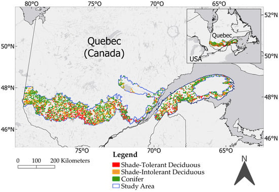
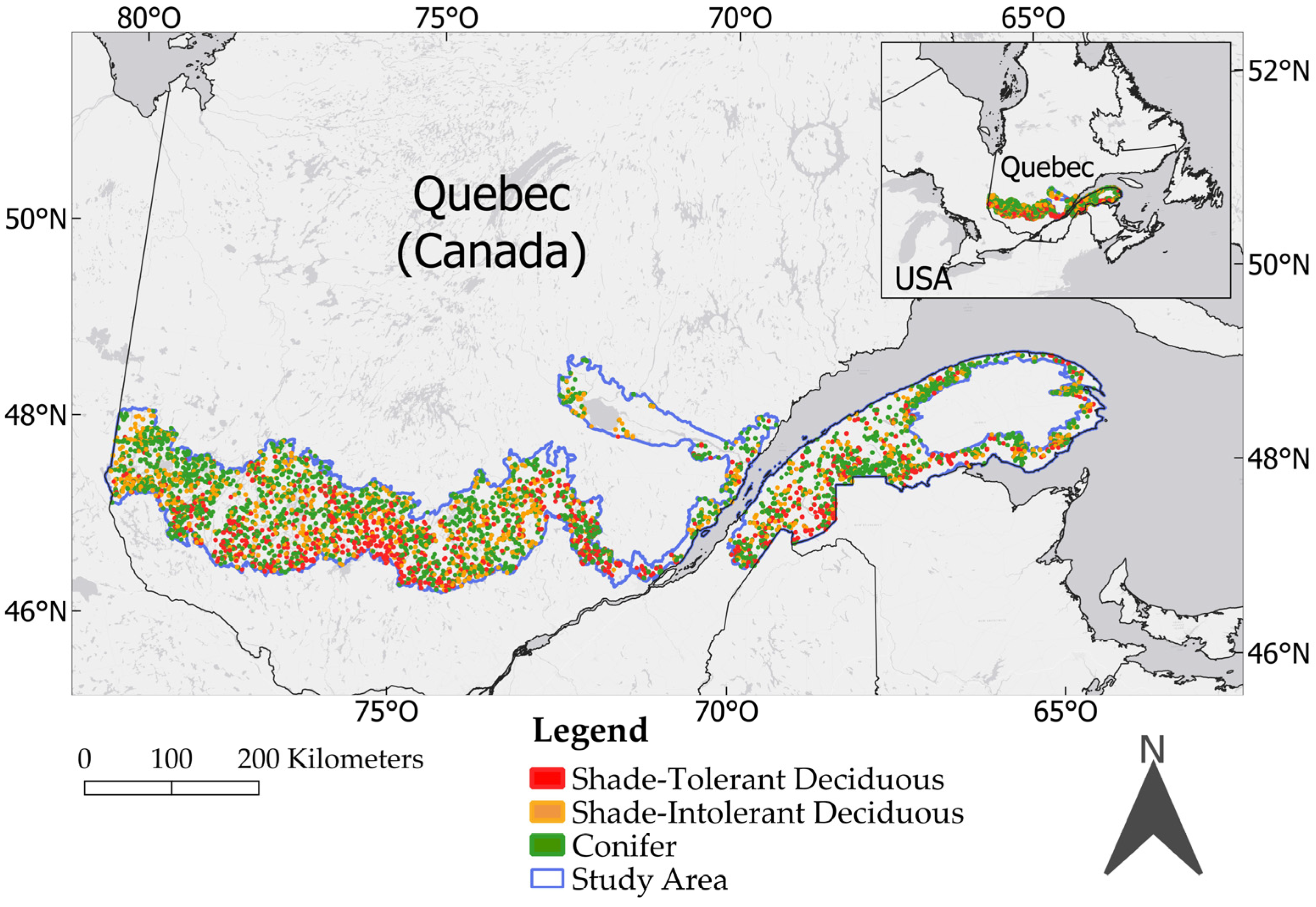
The study area (94,800 km²) is located within the bioclimatic domain of the balsam fir-yellow birch forest, which crosses the southern middle of Quebec from west to east (Figure 1) [45]. It extends between the 47th and 49th parallels. The elevation is relatively low, with less than 500 m in altitude, and the terrain is generally gently undulating. Annual precipitation ranges between 1100 and 1600 mm, with 30% falling as snow. The average temperature ranges from 0 to 2.5 °C, and the annual growing season lasts for 160 to 170 days [46,47]. The area includes stands of coniferous, mixed, and deciduous species, primarily dominated by Abies balsamea, Picea mariana, Betula papyrifera, Betula alleghaniensis, Populus tremuloïde and Acer saccharum. Within the study area, coniferous and shade-intolerant deciduous stands are managed as even-aged forests in public forests, while shade-tolerant stands are managed as irregular forests [48].

Figure 1. Field ground sample plots distribution by stand type (color dots) in the balsam fir-yellow birch forest of Quebec (study area).

This area represents the southernmost bioclimatic zone covered by the LiDAR Dendrometric Map and serves as the boundary between coniferous and mixed deciduous forests. This makes it the logical choice for conducting the study due to its significant proportion of stands dominated by deciduous species.

2.2. Data

2.2.1. Airborne LiDAR Data and Basal Area Prediction (Predicted Basal Area)

The predicted basal area tested in this study is derived from the LiDAR Dendrometric Map (LDM). Developed by the Ministry of Natural Resources and Forest (MNRF), Quebec, QC, Canada, the LDM provides predictions of essential forest attributes, including the basal area (BA) of merchantable trees (DBH > 9.0 cm), which is the focus of this study. The LDM predicts the basal area from the following method:

-

The basal area (BA) prediction process follows a similar method to that described in Leboeuf et al. (2022) for the volume prediction [17], where

-

BA is derived from a form factor, dominant height, and volume prediction.

-

Predictions are generated using a linear parametric model that incorporates independent variables derived from LiDAR and ecoforest map data.

-

LiDAR data acquisition in the study area took place between 2011 and 2020 during leaf-on periods.

-

Several sensors were used for data collection, with pulse density ranging from 2 to 6 points per square meter.

-

Variable selection was carried out using stepwise linear regression.

-

Basal area predictions are available at a 5 m × 5 m raster scale.

-

Known independent variables, including LiDAR-derived, MNRF custom-generated, and ecoforest map variables, are presented in Section 2.2.3 (independent variables).

2.2.2. Ground Sample Plots (Observed Basal Area)

To test the accuracy of the predicted basal area, a network of ground sample plots from the MRNF was used for the comparison. These plots include permanent plots, which are revisited periodically to track stand evolution, and temporary plots, which are specifically established for 10-year inventory. Each of these circular plots, measuring 400 m² (0.04 ha) of 11.28 m radius, includes data on tree count, average stand height, and for each tree, the diameter at 1.3 m from the ground (DBH) and tree species [49,50,51,52]. The study focuses on the inventory data collected between 2006 and 2020, covering the 4th and 5th decade inventories.

To ensure an accurate comparison of the BA between the ground sample plots and the LDM results, the ground sample plots had to meet six criteria.

• LiDAR coverage: The ground sample plots must be located in an area covered by LiDAR airborne data.
• Measurement timeframe: The selected plots must have been measured no more than five years before or after the LiDAR acquisition date.
• Absence of natural disturbances: No natural disturbances (e.g., windthrow events, storms, insect outbreaks) must have occurred between the LiDAR acquisition and their field measurement.
• Absence of human intervention: The plot must not have undergone any human interventions (e.g., logging, thinning, other silvicultural treatments) between the LiDAR acquisition and their field measurement.
• Stand attributes: The selected plots must have been established in productive forest stand of 7 m or more in height.
• A ≤3.57 m positional accuracy, ensuring co-registration with the LiDAR data [49,50,51,52].

Using these criteria, 12,506 plots were selected to represent three stand types across the study area (shade-tolerant deciduous, shade-intolerant deciduous and conifers) (Figure 1, Table 1). The stand types were established based on the main species indicated in the ecoforest map [53]. Yellow birch, sugar maple, red maple, and ash comprise the class of shade-tolerant deciduous. Aspen and white birch constitute the class of shade-intolerant deciduous. Spruce, larch, pine, fir, and cedar form the class of conifers. Finally, the basal area of each plot (observed value for the analysis) was calculated by summing the basal areas of all trees within it. We will refer to this reference value as the “observed basal area” in the remainder of the paper.

Table 1. Distribution of plots by stand type and observed basal area.

Stand Type	Number of Plots	Mean Basal Area (m2/ha)
Shade-tolerant deciduous	2590	24.22 (0.18–85.56)
Shade-intolerant deciduous	3217	23.77 (1.15–61.51)
Conifers	6699	24.62 (0.20–107.52)
Total	12,506	24.32 (0.18–107.52)

The bottom row, shown in bold, represents the total of the three stand types.

To ensure an adequate sample size, the literature suggests a minimum of 375 plots of 0.04 ha per stand type to achieve stability in the results [54] and the applied selection criteria allowed this threshold to be exceeded for all stand types (Table 1).

2.2.3. Independent Variables

Independent variables in the study are split into two groups: those used to build the LiDAR Dendrometric Map (LDM) [13,18,53] and additional data sources aimed at improving the accuracy of basal area prediction.

The source data for the LDM were provided by the MNRF and include LiDAR-derived, MNRF custom-generated, and ecoforest map variables. Details on LiDAR data acquisition parameters are presented in Section 2.2.1. (airborne LiDAR data and basal area prediction (predicted basal area)). The LiDAR Dendrometric Map (LDM) is produced using a standardized, province-wide workflow based on a fixed set of LiDAR-derived summary metrics [17]. This operational pipeline is designed to ensure consistency across all LiDAR acquisitions in Quebec and therefore does not incorporate additional point cloud-level descriptors such as voxel metrics, individual-tree segmentation, or extended height-percentile distributions. In this study, we relied on the metrics generated by the existing LDM workflow, as our objective was to evaluate and improve the predictive performance of the operational product rather than modify its underlying LiDAR processing chain.

Selection of the additional variables followed criteria of geolocated availability, continuous numerical type, coverage across the entire study area, and ability to explain differences or similarities between stand types. The additional set includes species composition from the MNRF ecoforest map, climatic data (1981–2010 mean) derived from geographical location and the BIOSIM software tool (version BIOSIM 9) [31,55], as well as geographic coordinates (latitude, longitude). These additional datasets are derived from the ecoforest map database [53].

Table 2 contains a detailed description of all variables.

Table 2. Description and value ranges of independent variables used in the study.

Variable	Description	Values
DENS_CLASS *12347	Canopy density. Calculated as the proportion of LiDAR points that do not reach the ground (%).	0 to 95
DH *23457	Dominant height. Average height of the highest LiDAR return in each 5 × 5 m pixel within the 11.26 m plot (m).	0.96 to 29.33
H_CLASS *1234567	Height above ground of the tallest tree. LDM polygon 1 m scale classification computed from DH (m).	4 to 30
LGDH *	Log10(DH).
RDI *	Relative density index indicating stand quality [17].	0.001 to 1.212
R_RDI_DH *1234567	RDI/DH.
LGRDI *234567	Log10(RDI).
FF10 *234567	Form factor used to estimate basal area from volume and dominant height. Predicted with LiDAR Dendrometric Map.	0 to 0.415
N10 *12347	Estimated number of merchantable stems (trees) per hectare. Predicted with LiDAR Dendrometric Map.	0 to 2939
ALTITUDE *	Altitude (m) derived from digital terrain model.	0 to 890
LGALT *234567	Log10(ALTITUDE).	0 to 2.938
dSPEC_PR *1234567	Dominant species of the stand according to the ecoforest map where PR correspond to EN (Picea mariana), EB (Picea glauca), SB (Abies balsamea), BP (Betula papyrifera), BJ (Betula alleghaniensis), ES (Acer saccharum), EO (Acer rubrum), PE (Populus spp.), TO (Thuja occidentalis), PG (Pinus banksiana), AF (other deciduous species), AR (other coniferous species), ML (Larix laricina), FN (Fraxinus nigra) and PB (Pinus strobus). Factor/categorical value.	“EN”, “EB”, “SB”, “BP”, “BJ”, “ES”, “EO”, “PE”, “TO”, “PG”, “AF”, “AR”, “ML”, “FN”, “PB”
pXXX 1234567	Proportion of the basal area in the stand cover by species (%), where XXX corresponds to WSP 1467 (Picea glauca), BSP 146 (Picea mariana), BFI 23467 (Abies balsamea), JPI 147 (Pinus banksiana), TAM 47 (Larix laricina), FSPL 2347 (fir, spruce, pine, and larch), WPI 7 (Pinus strobus), OPI 7 (other pine species, mostly Pinus resinosa), OCON 1234567 (other conifers, mostly Thuja occidentalis), TCON 12347 (all conifers), WBI 13467 (Betula papyrifera), YBI 12347 (Betula alleghaniensis), ASPE 1467 (Populus spp.), RMA 47 (Acer rubrum), SMA 347 (Acer saccharum), ODEC 47 (other deciduous, mostly Quercus rubra, Fraxinus nigra and Fagus grandifolia).	0 to 100
DEGRE_DAY 1347	Annual sum of daily average temperatures above 5 °C (Tavg − 5) for days where Tavg > 5 °C (°C).	977.9 to 1660.5
PRECI_GRS 1467	Total precipitation during the growing season (GRS) (mm).	380.3 to 664.7
PRECI_SNOW 147	Annual total of snow precipitation converted to liquid equivalent, considering only days where Tavg < 0 °C (mm).	229.9 to 574.2
PP_SNOW 1347	Proportion of total precipitation in the form of snow (%).	27.95 to 45.75
TMIN_AN 34567	Annual average of daily minimum temperatures (°C).	−6.34 to −0.60
TMOY_AN 4	Annual average temperature (°C).	−0.42 to 4.11
TMAX_AN 134567	Annual average of daily maximum temperatures (°C).	5.35 to 9.64
TMOY_GRS 1234567	Average temperature during the growing season (°C).	12.49 to 14.84
TMOY_JULY 34567	Average temperature in July (°C).	14.26 to 18.51
FF_TOT 14567	Total number of frost-free days (Tmin > 0 °C).	137 to 193
CONSE_FF 467	Number of consecutive frost-free days (Tmin > 0 °C).	49 to 137
DAY_GRS 467	Number of days in the growing season (GRS).	115 to 166
FDAY_FF 1467	First day of the consecutive frost-free days period (Julian day).	135 to 179
VPD_UTI 1347	Cumulative vapor pressure deficit for June, July, and August (Julian days 152 to 243) (mbar).	1075 to 1552
ARID_TOT 14567	Sum of monthly water deficits based on the difference between monthly precipitation and Thornthwaite potential evapotranspiration (0 if negative) (cm).	0.49 to 5.88
RADIA_T 47	Annual sum of energy emitted by solar radiation (MJ/m2).	4581 to 5415
RADIA_GRS 47	Energy emitted by solar radiation during the growing season (GRS) (MJ/m2).	2327 to 2921
LATITUDE 1234567	Geographic coordinate that specifies the north–south position of a point on Earth (dd.ddddd).	46.66 to 49.22
LONGITUDE 134567	Geographic coordinate that specifies the east–west position of a point on Earth (dd.ddddd).	−79.52 to −64.32

* Variables used to build LDM. ^1234567 Details on the meaning of the index numbers are provided in Section 3.2.

LGDH and RDI are not considered in variable selection, because they are directly correlated to other variables: LGDH to DH and RDI to LGRDI.

The relative density index (RDI) and the form factor (FF10) are custom variables generated by the MNRF. RDI is calculated by first calibrating a self-thinning line using quantile regression on the number of stems taller than 5 m from ground sample plots. RDI values are then derived by taking the ratio of the observed stem count to the predicted values from the self-thinning line. Finally, a log-linear model with LiDAR-derived metrics is developed to generate an RDI raster for the study area [17]. The form factor is generated using a bank of measured taper coefficients for each species and then adapted to a 5 m × 5 m raster [56].

Species composition follows the MNRF ecoforest map of Quebec, which is based on the photo-interpretation of high-resolution aerial imagery. Trained photo-interpreters delineate forest stands based on stand resemblance, and species distribution is assessed using basal area cover proportion [57].

Geolocated meteorological data are generated through the BIOSIM software tool [31,55], which was initially developed to analyze insect behavior. BIOSIM utilizes historical meteorological data collected by weather stations across Canada and extrapolates weather trends between these stations to generate geolocated climate data.

Geographical coordinates consist of the latitude and longitude of the center of each sample plot.

The use of the variables is presented in Section 2.3.2. (identification of basal area predictors).

2.3. Data Analysis

2.3.1. Assess the BA Accuracy of the LDM

The accuracy assessment of the LDM for predicting basal area (predicted BA) was conducted at the plot level using ground sample plots for comparison (observed BA). To ensure consistency with the ground sample plots, the 5 m × 5 m raster data were converted to match the format of the 11.28 m circular plots. Predicted BA for each plot was obtained by overlaying the plots onto the raster pixels and calculating a weighted average of the BA values from the pixels with centroids inside the plot.

Once the data were adjusted to the appropriate format, analysis was performed using R Studio statistical software (version 2023.09.1+494). Accuracy was assessed through statistical analysis using the coefficient of determination (R²) (Equation (1)), bias (Equation (2)), root mean square error (RMSE) (Equation (3)), mean absolute error (MAE) (Equation (4)), and the fraction of variance of the “expected response” (r²_ER) (Equation (5)) [58].

$${\mathrm{R}}^2=1-{\displaystyle \frac{{\sum }_{i=1}^n{\left(y_i-x_i\right)}^2}{{\sum }_{i=1}^n{\left(\overline{x}-x_i\right)}^2}}$$

(1)

$$\mathrm{b}\mathrm{i}\mathrm{a}\mathrm{s}={\displaystyle \frac{1}{n}}\sum _{i=1}^n\left(y_i-x_i\right)$$

(2)

$$\mathrm{R}\mathrm{M}\mathrm{S}\mathrm{E}=\sqrt{{\displaystyle \frac{1}{n}}\sum _{i=1}^n{\left(y_i-x_i\right)}^2}$$

(3)

$$\mathrm{M}\mathrm{A}\mathrm{E}={\displaystyle \frac{{\sum }_{i=1}^n\left|y_i-x_i\right|}{n}}$$

(4)

$${{\mathrm{r}}^2}_{\mathrm{E}\mathrm{R}}={\displaystyle \frac{({\sum }_{i=1}^n\left(y_i-\overline{y}\right)\left(x_i-\overline{x}\right){)}^2}{{\sum }_{i=1}^n(y_i-\overline{y}{)}^2{\sum }_{i=1}^n(x_i-\overline{x}{)}^2}}$$

(5)

where n is the number of field plots, x_i is the ground field inventory (observed value), $\overline{x}$ is the mean of the field inventory, y_i is the predicted value and $\overline{y}$ is the mean of the predicted value.

To evaluate the influence of species composition on model performance, stands were analyzed by stand types and dominant species. This stratification allowed the assessment of how species dominance affected the effectiveness of the LiDAR Dendrometric Map (LDM). Predictions were evaluated for stands dominated by Betula papyrifera (white birch), Populus spp. (aspen), Betula alleghaniensis (yellow birch), Acer rubrum (red maple), Acer saccharum (sugar maple), Fraxinus spp. (ash), Picea glauca (white spruce), Picea mariana (black spruce), Larix laricina (larch), Pinus strobus (white pine), Pinus banksiana (jack pine), Abies balsamea (balsam fir), and Thuja occidentalis (white cedar). In addition, stands were grouped into three stand types (coniferous, shade-intolerant deciduous, and shade-tolerant deciduous) to examine differences in model performance across general stand categories. After assessing the accuracy of the LDM, the next step was to identify the most relevant predictors for modeling basal area. Section 2.3.2 describes the feature selection procedures used to construct the predictor subsets.

2.3.2. Identification of Basal Area Predictors (Independent Variables)

Feature selection is an important step in model improvement. Using fewer variables is more restrictive, as it limits the model to only the most critical predictors, potentially simplifying the model but risking the loss of valuable information. On the other hand, including more variables is less restrictive, providing the model with a broader range of data, which can capture more complex patterns but may also introduce noise or redundancy [59]. To select the optimal predictors among the variables presented in Table 2, three variable selection methods were used to identify subsets of relevant variables for the development of the predictive model: stepwise forward and backward selection, the Boruta method, and the Least Absolute Shrinkage and Selection Operator (Lasso). Feature selection for each method was performed in R Studio.

Stepwise forward and backward selection [60]: We implemented both forward selection (adding variables one by one) and backward elimination (removing less significant variables) using the Akaike Information Criterion (AIC) to optimize model fit. The process followed these steps:

• Base model: A linear regression model was initialized with only an intercept.
• Subsets models: Models including similar predictors subsets were defined.
• Stepwise selection: For each subset, the step() function in R studio was used to iteratively add or remove variables based on AIC, balancing model complexity and predictive power. The most significant variables from each subset were retained.
• Final selection: After analyzing the individual subsets, a final stepwise selection was performed on the combined set of shortlisted variables to further refine the model. This final iteration ensured that only the most predictive and non-redundant variables were retained.

Boruta method [61]: Boruta is a Random Forest-based wrapper algorithm that identifies predictors whose importance exceeds that of permuted “shadow” variables. We applied Boruta using the Boruta R studio package and retained variables classified as confirmed after applying the TentativeRoughFix procedure. The resulting ranked list provided an alternative subset used to assess the robustness of the stepwise selection.

Lasso regression [62,63]: Lasso performs variable selection by shrinking some coefficients to zero through an L1 penalty. Using the glmnet package, we identified two subsets based on λ_min and λ_1se obtained via cross-validation. These subsets were used to evaluate whether a regularization-based method selected predictors consistent with the stepwise approach. Four primary subsets were generated from the feature selection methods: one from stepwise selection, two from Lasso (λ_1se and λ_min), and one from Boruta selection. Additional subsets were constructed based on the variable importance rankings from Lasso and Boruta to match the number of variables selected by stepwise and Lasso λ_1se. This procedure resulted in three additional subsets, for a total of seven subsets. These subsets were later compared in the modeling approaches section to evaluate their performance under the best-performing modeling approach. They were generated to compare the performance of different feature selection strategies based on distinct statistical principles.

Stepwise selection, Boruta, and Lasso each identify relevant predictors using different criteria (AIC optimization, Random Forest importance, and L1 regularization, respectively). Creating multiple subsets allowed us to evaluate the stability of selected predictors across methods and to assess whether model performance was sensitive to the choice of feature selection technique. Additional subsets with matched variable counts were included to ensure fair comparisons across methods.

Once the predictor subsets were generated, we evaluated their predictive performance using three modeling approaches, described in Section 2.3.3.

2.3.3. Modeling Approaches

Three modeling approaches were applied to the variables selected through the stepwise method: linear parametric models, non-linear parametric models, and automated machine learning. Each model was trained on 80% of the dataset and evaluated on the remaining 20% to assess predictive accuracy.

(1)

Linear parametric models fitted a linear regression with observed basal area values as the response variable and variables selected by the stepwise method cited in Section 2.3.2 above as the explanatory variable. The model can be expressed as follows:

$$Y=A\times X+B\times Z+\epsilon$$

(6)

where Y is the dependent variable (observed basal area), X is the predicted basal area, Z is the explanatory variable, A and B are the general parameters of the equation and ε is the error term.

(2)

Non-linear parametric models [64], quadratic, logarithmic, square root, and reciprocal applying the same methodology as in method one. Although fully parameterized multivariate non-linear models are typically expressed in a multiplicative form (y = a₀ x₁^a1 x₂^a2 … x_p^ap + ε), the non-linear models used in this study follow an additive structure with non-linear transformations of individual predictors. These transformations provide flexible non-linear responses while maintaining interpretability and avoiding the complexity of fitting full non-linear multiplicative models. The performance of each model was tested, and the linear model and the best-performing non-linear model were retained for comparison with the other approach.

(3)

Using automatic machine learning H2O(H2OAutoML) with R studio package H2O (version 3.42.0.2) [65]. It is an open-source tool for automating the predictive analytics workflow. It is widely used in academia and in industry as well [66]. The H2O AutoML tests different models such as a generalized linear model (GLM), a default Random Forest (DRF), a gradient boosting machine (GBM), a near-default Deep Neural Nets (DNNs) and Stacked Ensemble Model (SEM) that integrates the previous models to determine the optimal combination of prediction algorithms all in one function [67]. The AutoML search was constrained to a 60 s runtime to ensure consistent and reproducible model exploration across all stand types. Preliminary tests indicated that this duration allowed AutoML to evaluate a sufficiently diverse set of candidate models while maintaining stable performance rankings. Model evaluation relied on 5-fold cross-validation, and hyperparameter optimization was performed using H2O’s random search strategy with early stopping based on the convergence of cross-validated RMSE. Under these conditions, AutoML typically generated between 20 and 30 models, from which the final Stacked Ensemble was constructed using the top-performing base learners.

Model performance was compared across the three approaches and against the LDM. The best-performing approach was subsequently applied to the six additional variable subsets generated through Lasso and Boruta feature selection in order to identify the most effective feature selection strategy.

3. Results

3.1. LiDAR Dendrometric Map Accuracy Assessment

For practical purposes (AAC calculations, harvest planning, etc.), the forest inventory must provide useful information by species or groups of species. Table 3 displays the average observed and predicted basal area for each of the three stand types and dominant species along with the computed statistics.

Table 3. Performance results of the LiDAR Dendrometric Map sorted by stand types and main tree species composition.

Stand Type	Species	N	BAObs	BAPred	Bias	MAE	RMSE	R2	r2ER
			(m2/ha)	(m2/ha)	(m2/ha)	(m2/ha)	(m2/ha)
Shade-tolerant deciduous		2590	24.22	27.01	2.79	6.01	7.43	0.246	0.103
	Yellow birch	1430	24.48	26.89	2.41	5.96	7.43	0.243	0.151
	Red maple	337	23.99	24.67	0.68	5.52	6.94	0.363	0.332
	Sugar maple	802	24.04	28.46	4.41	6.35	7.65	0.226	0.177
	Ash	21	16.97	17.40	0.43	4.84	5.66	0.400	0.190
Shade-intolerant deciduous		3217	23.77	24.43	0.66	5.30	6.83	0.469	0.461
	White birch	2192	23.76	24.82	1.06	5.09	6.43	0.454	0.434
	Aspen	1025	23.79	23.61	−0.18	5.74	7.61	0.498	0.498
Coniferous		6699	24.62	23.26	−1.36	5.27	7.38	0.534	0.513
	White spruce	388	27.19	24.15	−3.04	6.10	7.87	0.509	0.419
	Black spruce	2194	21.36	21.65	0.29	4.30	5.70	0.603	0.602
	Larch	109	21.14	22.98	1.84	4.83	6.69	0.560	0.517
	White pine	65	23.34	23.86	0.52	6.28	8.11	0.412	0.409
	Jack pine	515	20.55	21.35	0.80	4.43	5.65	0.559	0.540
	Balsam fir	3047	26.21	24.01	−2.20	5.39	7.41	0.514	0.464
	White cedar	381	34.78	28.14	−6.65	10.08	14.26	0.271	0.057

Bold values indicate the stand level summaries.

Bias indicates that, on average, the LDM underestimated the basal area for coniferous stands while it overestimated it for the deciduous stands. Shade-tolerant deciduous stands showed slightly higher bias (2.79 m²/ha) and MAE (6.01 m²/ha) than the other two stand types. Although the absolute RMSE was higher in coniferous stands, the relative error (RMSE%) remained slightly higher in shade-tolerant deciduous stands (30.6%) compared with coniferous (30.0%) and shade-intolerant deciduous stands (28.7%). R² and the r²_ER showed higher results for the coniferous (0.534) and shade-intolerant deciduous (0.469) stands than for the shade-tolerant deciduous stands (0.246).

The stands dominated by sugar maple and yellow birch showed particularly poor performance, with R² values of 0.226 and 0.243, and overestimations of 4.4 m²/ha and 2.4 m²/ha, respectively. Stands dominated by white cedar also performed poorly, with an R² of 0.271 and an underestimation of 6.6 m²/ha.

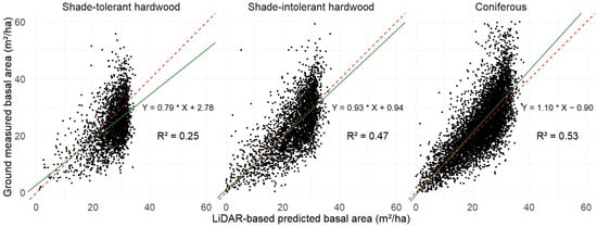
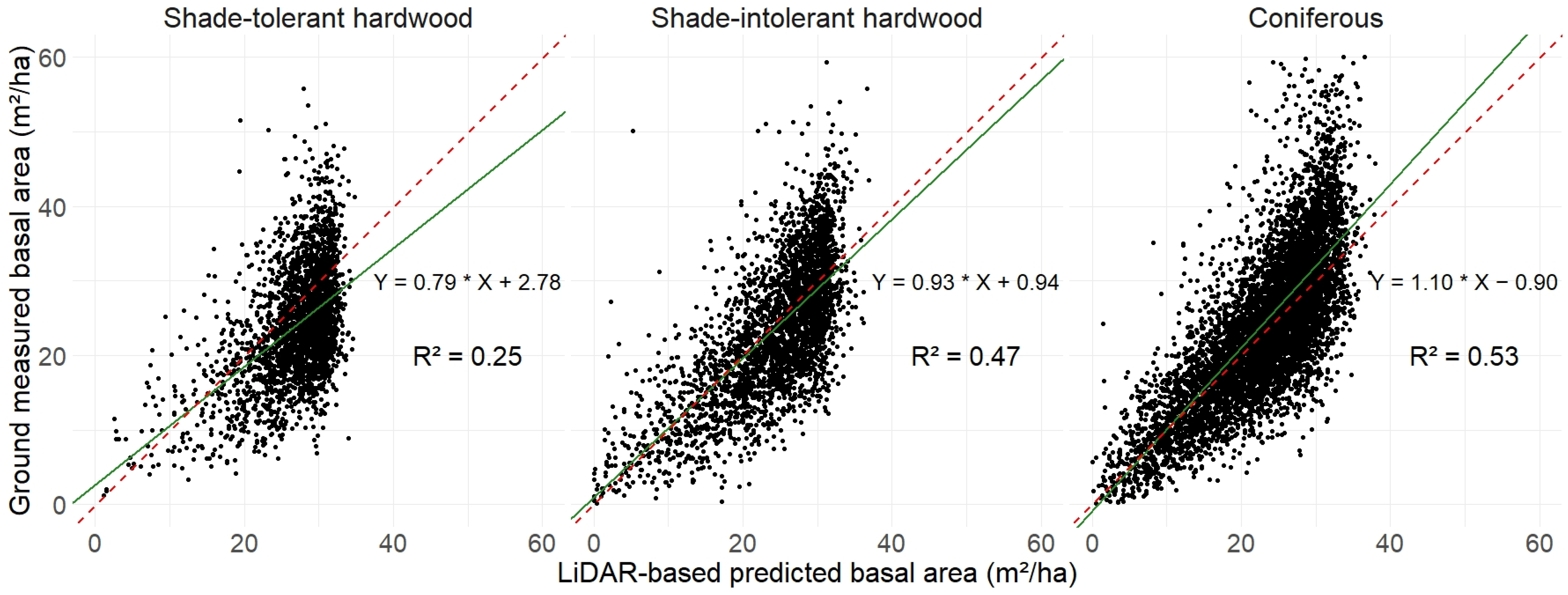
Figure 2 illustrates the relationship between ground-observed data and the LiDAR Dendrometric Map. As the parameter approaches 1, the R² value increases, indicating more accurate results.

Figure 2. Correlation between ground sample plots measured basal area and predicted basal area from the LiDAR Dendrometric Map for the three stand types. The red dashed line represents the 1:1 ratio, while the green line indicates the fitted linear relationship.

Figure 2 illustrates that shade-tolerant deciduous stands exhibit a correlation deviating from the 1:1 line, as indicated by the equation Y = 0.79x + 2.78 (a). Conversely, shade-intolerant and coniferous stands demonstrate regressions closer to the 1:1 line, with equations of Y = 0.93x + 0.94 (b) and Y = 1.10x − 0.90 (c), respectively.

3.2. Independent Variables Analysis

3.2.1. Stepwise Selection Method

A total of 25 variables were retained, including localization data, species composition percentages, and meteorological variables. The selected variables are indicated with the index 1 in Table 2.

3.2.2. Boruta Method

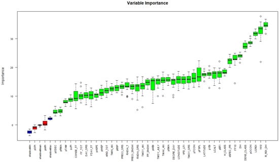
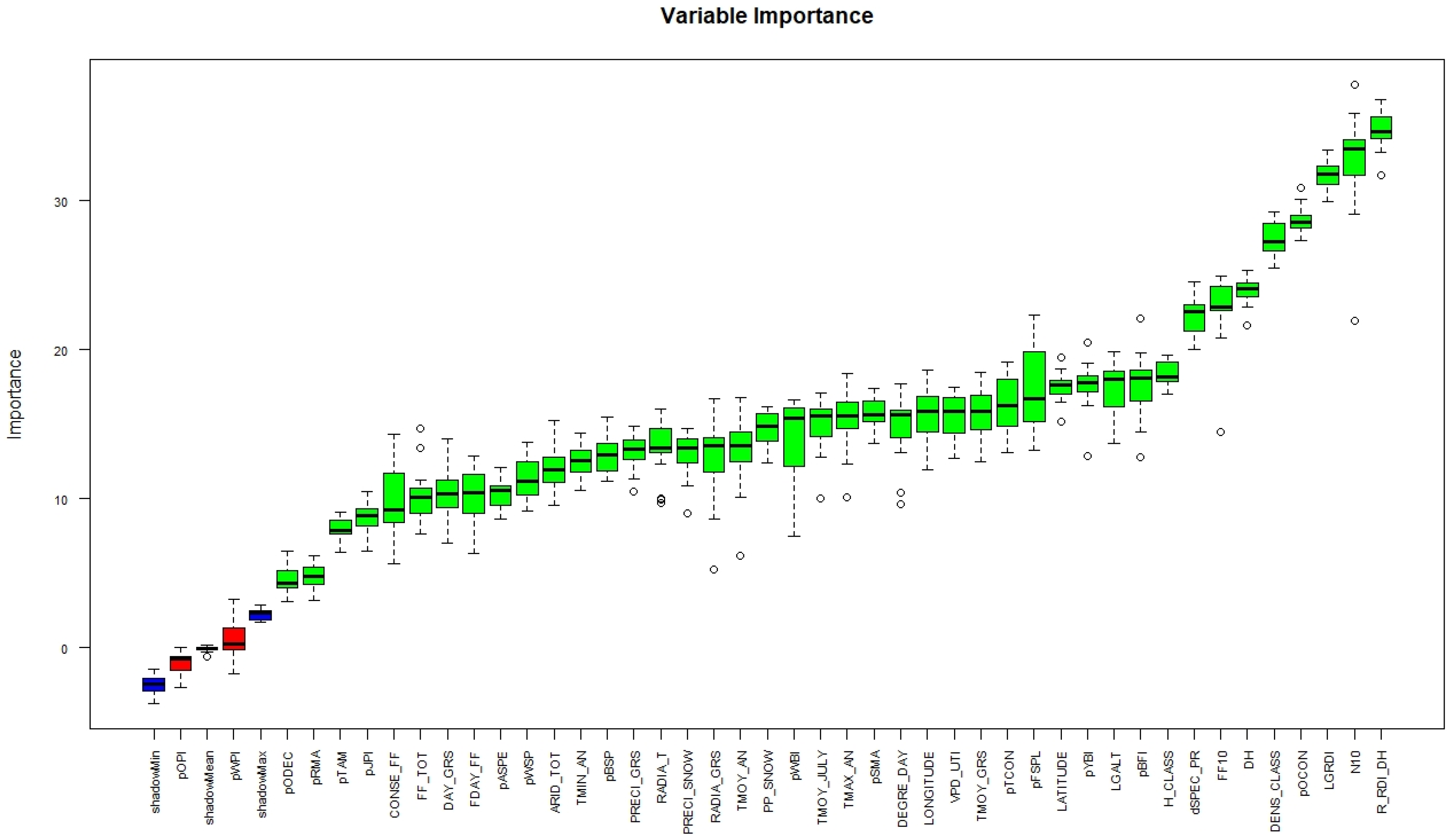
Figure 3 depicts the Boruta variable importance chart. Blue boxes represent the maximum, mean, and minimum Z score of a shadow attribute. Green and red boxplots represent Z score of confirmed and rejected variables respectively. Out of the 44 variables, two were rejected (pOPI and pWPI) and 42 were confirmed.

Figure 3. Distribution of variables according to their degree of importance as judged by the Boruta method. Green: confirmed important variables; red: rejected variables; blue: shadow features used as random benchmarks.

3.2.3. Lasso Method

Figure 4 and Table 4 illustrate the results obtained from the Lasso method.

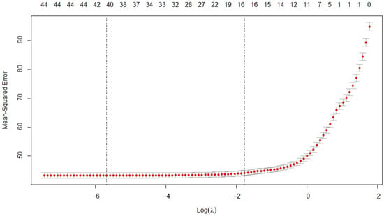
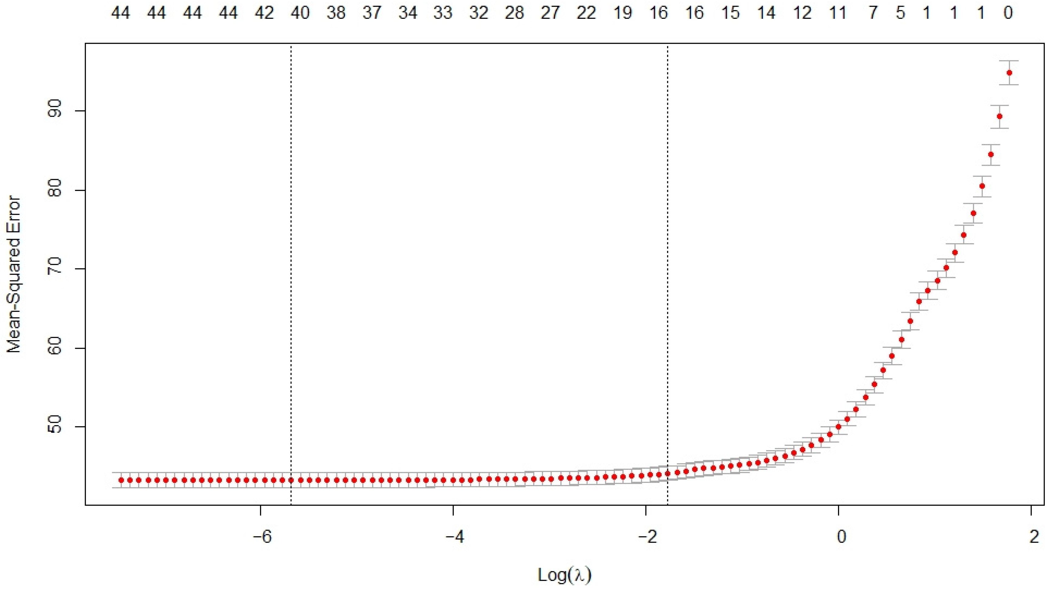
Figure 4. Lasso-generated graph illustrates the optimal number of variables (top ax) to incorporate into the model, between the available variables. The curve represents the average prediction error across folds, with vertical bars indicating ±1 standard error. The dashed vertical lines indicate the optimal values of λmin and λ1se.

Table 4. Best 25 variables selected by Lasso regression ranked by absolute coefficient value.

Rank	Variable	Coefficient	Abs (Coefficient)
1	R_RDI_DH	1037.24	1037.24
2	FF10	15.93	15.93
3	LGALT	−2.60	2.60
4	TMOY_GRS	−2.30	2.30
5	TMAX_AN	1.70	1.70
6	LATITUDE	1.01	1.01
7	LGRDI	−0.92	0.92
8	H_CLASS	−0.63	0.63
9	ARID_TOT	−0.63	0.63
10	TMOY_JULY	−0.38	0.38
11	TMIN_AN	−0.32	0.32
12	pOCON	0.24	0.24
13	DH	−0.12	0.12
14	LONGITUDE	0.12	0.12
15	dSPEC_PR	0.11	0.11
16	FF_TOT	−0.10	0.10
17	DAY_GRS	0.09	0.09
18	pWSP	0.07	0.07
19	CONSE_FF	0.06	0.06
20	pBFI	0.05	0.05
21	pWBI	0.04	0.04
22	pBSP	0.04	0.04
23	pASPE	0.03	0.03
24	PRECI_GRS	−0.03	0.03
25	FDAY_FF	−0.03	0.03

The two vertical lines correspond to λ_min, which minimizes the cross-validated mean squared error (MSE) and retains more predictors, and λ_1se, within one standard error of the minimum, producing a more parsimonious model with fewer variables. According to these values, the optimal number of variables falls within the range of 16 to 43.

The Lasso variables were ranked according to their λ_min coefficients, which represent the expected change in the response variable for a one-unit increase in the corresponding predictor, holding all other variables constant. Using λ_min instead of λ_1se allows the ranking of additional variables beyond the first 16 (up to 43), since the λ_1se model sets the remaining coefficients to zero, facilitating comparison with other feature selection methods. Because variables were set on the same scale, the absolute values of the coefficients directly correlate with their importance in the model. Table 4 shows the variable rank by coefficient value.

Table 4 presents the ranking of the 25 most influential variables identified by the Lasso regression; beyond this point, coefficient magnitudes gradually decreased from PP_SNOW (0.03) to N10 (−0.0003). The only variable with a coefficient of 0 is TMOY_AN, which means it was not considered to have any influence on the model and was excluded from the Lasso selection.

Because each feature selection method produced a different number of selected variables, subsets were created to allow a fair comparison by using the same number of variables across methods. Since the stepwise method does not provide a variable ranking, subsets were generated only for Boruta and Lasso. Three rankings were considered: the 16 best variables according to Lasso λ_1se (within one standard error of the minimum), the 25 best variables corresponding to the number selected by the stepwise method, and the corresponding number of variables selected by each method. This procedure resulted in seven subsets, with the selected variables for each method presented in Table 2 along with their respective superscript.

^1. 

Stepwise method, 25 selected variables

^2. 

Boruta method, best 16 variables

^3. 

Boruta method, best 25 variables

^4. 

Boruta method, 42 selected variables

^5. 

Lasso method, λ_1se 16 variables

^6. 

Lasso method, best 25 variables

^7. 

Lasso method, λ_min 43 variables

3.3. Model Improvement with Three Approaches

3.3.1. Linear Parametric, Non-Linear Parametric and H2O AutoML Models

For comparison, all-new modeling approaches were developed using the same set of variables selected through the stepwise backward selection method [17].

Linear Model

Equation (7) displays the results of the optimized linear model.

$$\begin{array}{ll}BAcorrected=& 3.64+959.03\times R\_RDI\_DH-1.57\times TMOY\_GRS+1.39\times TMAX\_AN\\ & +1.31\times LATITUDE-0.57\times H\_CLASS+0.16\times pOCON-0.13\times ARID\_TOT\\ & +B\times factor\left(dSPE{C}_{PR}\right)+{\displaystyle \sum _i}{\beta }_i{X}_i\end{array}$$

(7)

where BAcorrected is the prediction of the model, factor(dSPEC_PR) represents a coefficient B assigned to each species, which is only applied when that species is the dominant one in the stand. Other predictors are also present in the model but are not explicitly displayed in the formula due to their lower relative importance ${\sum }_{\mathit{i}}{\mathit{\beta }}_{\mathit{i}}{\mathit{X}}_{\mathit{i}}$. Results are shown in Table 5.

Table 5. New modeling approach performances using the stepwise variable selection, compared to the LiDAR Dendrometric Map, for all commercial stands and shade-tolerant deciduous stands.

Approaches	All Commercial Stands					Shade-Tolerant Deciduous Stands
	N	MAE	Bias	R2	r2ER	N	MAE	Bias	R2	r2ER
		(m2/ha)					(m2/ha)
LiDAR Dendrometric Map	2560	5.47	−0.02	0.456	0.456	515	6.03	2.70	0.266	0.134
H2O AutoML	2560	4.78	−0.05	0.598	0.596	515	5.13	0.01	0.312	0.310
Linear	2560	5.03	0.06	0.559	0.558	515	5.21	0.03	0.310	0.308
Quadratic	2560	5.06	−0.30	0.546	0.544	515	5.20	0.03	0.306	0.304

Blue is used in table to identify the initial model, which serves as the reference.

Non-Linear Model

Out of all the non-linear models tested, the quadratic regression model produced the best results. Equation (8) displays the optimized quadratic base on the same approach as the linear model.

$$\begin{array}{ll}BAcorrected=& -24.92+834.14\times R_{RD{I}_{DH}}+{ 23.68\times R_{RD{I}_{DH}}}^2-0.73\times H_{CLASS}+0.14\times pOCON\\ & -3.14\times TMO{Y}_{GRS}+0.55\times TMA{X}_{AN}+0.40\times ARI{D}_{TOT}+2.02\times LATITUDE\\ & +factor(dSPEC\_PR)+{\displaystyle \sum _i}{\beta }_i{X}_i\end{array}$$

(8)

The same notation and additional predictors as described in Equation (7) are used. Results are shown in Table 5.

H2O AutoML Model

The H2O AutoML function does not provide a detailed description of the best resulting model because its primary goal is to automate the model selection and tuning process rather than to generate interpretable model outputs. The best-performing model often corresponds to a Stacked Ensemble, which combines multiple base learners (e.g., GBM, DRF, DNN, GLM) to maximize predictive accuracy. This Ensemble Model integrates the predictions of several algorithms through a meta-learner, making the internal structure complex and not easily summarized in a single set of equations or coefficients.

The leaderboard indicates that the Stacked Ensemble Model achieved the highest performance among all AutoML candidates, followed by GBM, and outperformed DRF, DNN, and GLM. Results for the best model are presented in Table 5 under H2O AutoML.

For all three modeling approaches, the best performance for shade-tolerant species was achieved by training models exclusively on data from shade-tolerant deciduous stands, using the same input variables.

3.3.2. Comparing Models Performance: New Approaches vs. Initial Model

Table 5 shows that the H2O AutoML method achieved the best overall performance across both groups. For all commercial stands, r²_ER increased from 0.456 (LDM) to 0.598, with MAE reduced from 5.47 m²/ha to 4.78 m²/ha and bias remained close to zero (−0.05). For shade-tolerant deciduous stands, r²_ER improved from 0.134 to 0.310, MAE decreased from 6.03 m²/ha to 5.13 m²/ha, and bias was also minimized from 2.70 m²/ha to 0.01 m²/ha. Linear and quadratic models also provided considerable improvements, with the linear model performing slightly better for all commercial stands and shade-tolerant deciduous stands.

In order to further improve model performance, subsequent evaluations were conducted using the other variable subsets with the H2O AutoML, the best-performing modeling approach.

3.3.3. Testing the Variable Selection Impacts on the Best-Performing Model (H2O AutoML)

To select the inputs for automatic machine learning, a comparison between metric selection approaches was conducted and is presented in Table 6.

Table 6. Variable selection results: comparison of performance for Boruta, stepwise, and Lasso methods with different number of inputs.

Method	Number of Inputs	r2ER
Stepwise	25	0.5964
Boruta	25	0.5965
Lasso	43	0.5969

Based on the results presented in Table 6, increasing the number of input variables beyond 25 does not lead to any meaningful improvement in explained variance. All three feature selection methods (stepwise, Boruta, and Lasso) produced very similar predictive performance, with differences in r²_ER below 0.001. Given this equivalence, the stepwise method with 25 selected variables was retained for model development, as it provides comparable accuracy while relying on a more parsimonious and interpretable set of predictors.

3.3.4. Testing Best Model with Best Variable Selection

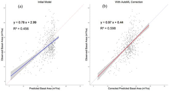
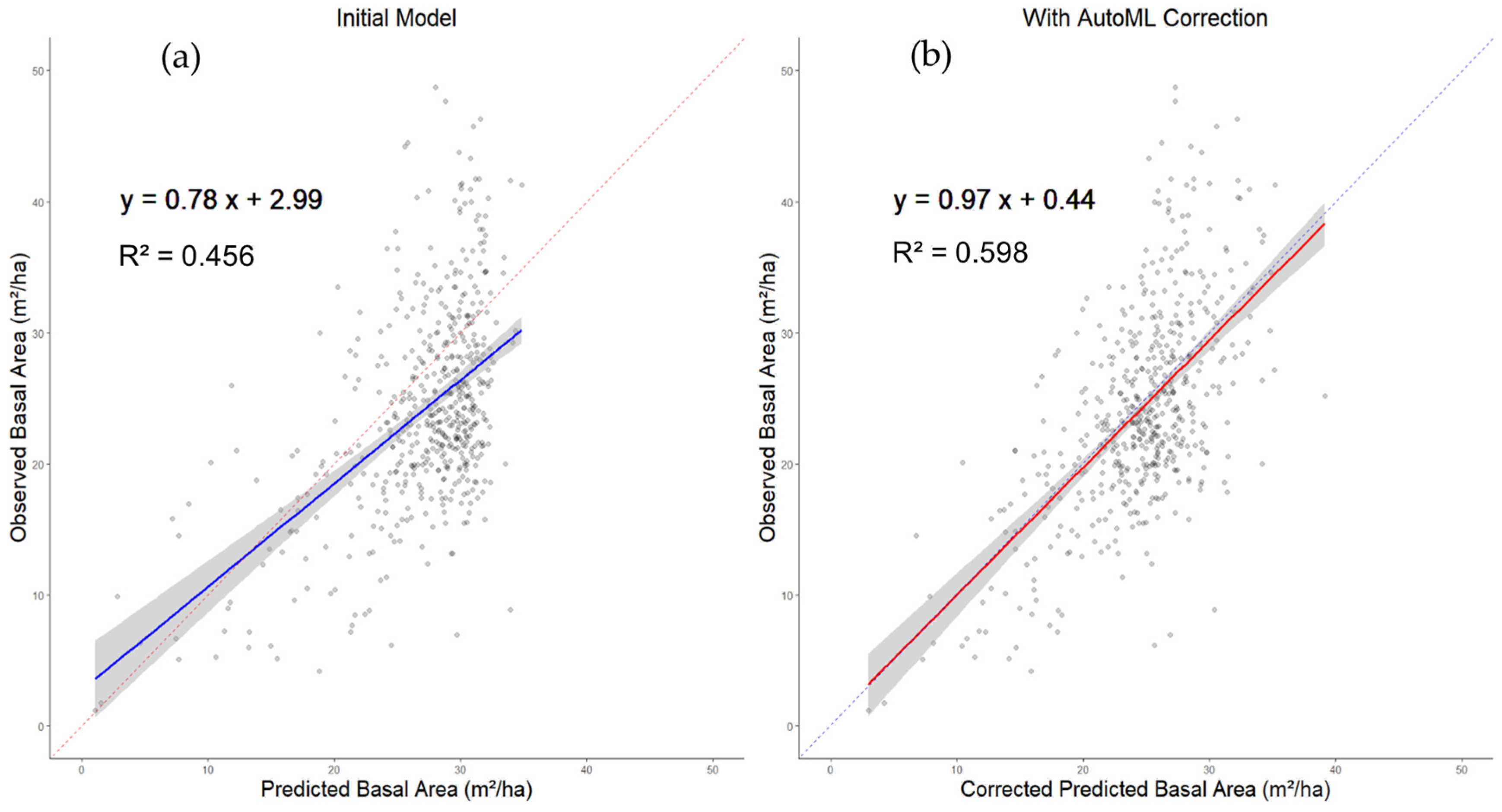
A graphical representation illustrating the correction’s impact using AutoML on the distribution of data, comparing observed and predicted basal area in shade-tolerant deciduous stands, is depicted in Figure 5.

Figure 5. Observed stand basal area as a function of the stand basal area predicted by initial model (a) and the corrected one following H2O AutoML method (b) in shade-tolerant deciduous stands situations. The dashed lines represent the 1:1 ratio, while the full lines (blue for the initial model and red for the AutoML-corrected model) indicates the fitted linear relationship.

We observe that the results are centered on the 1:1 line in the AutoML corrected model; however, the data points are still widely scattered around this line, highlighting the lack of accuracy.

Results for each stand type show the improvement from the initial model to the best model (Table 7). The test dataset is used for the comparison, which represents 20% of the total data, ensuring trustworthy results by using data that were not part of the model training.

Table 7. Performance results of the initial LiDAR parametric model and the best model issue with H2O AutoML correction on the test data by stand type.

		Initial Model					Best Model
Stand Type	N	Bias	MAE	RMSE	R2	r2ER	Bias	MAE	RMSE	R2	r2ER
Shade-tolerant deciduous	515	2.70	6.03	7.45	0.266	0.134	0.01	5.13	6.64	0.312	0.310
Shade-intolerant deciduous	624	0.96	5.31	7.07	0.468	0.455	0.42	4.81	6.37	0.559	0.557
Coniferous	1421	−1.43	5.33	7.70	0.539	0.516	−0.28	4.64	6.43	0.669	0.662
All commercial	2560	−0.02	5.47	7.50	0.456	0.456	−0.05	4.78	6.46	0.598	0.596

The bottom row, shown in bold, represents the total of the stand types above.

Improvements were observed across all stand types, with the most significant corrections seen in shade-tolerant deciduous stands in terms of bias, MAE and r²_ER. Coniferous stands received the most significant correction in terms of RMSE and R². Despite the improvements, shade-tolerant deciduous stands still exhibit a lower performance indicator than the other stands in the initial model.

4. Discussion

This project has provided essential confirmation that ALS-based approaches, such as the LDM developed by the Quebec government’s forest inventory program, still require refinement before they can be extended to temperate forests with complex stands, like those in the southern regions of Quebec. In particular, shade-tolerant deciduous stands have been identified as the main challenge requiring further research and development. The incorporation of geolocalized data independent of ground samples, together with the original metrics of the LDM, combined with the use of automated machine learning, has led to notable improvements. Although these enhancements have not yet yielded competitive accuracy for shade-tolerant deciduous stands, the approach developed in this project opens a new avenue for generating data that can be integrated with future advancements in the field. The approach adopted in this project lays the foundation for leveraging automated machine learning to fully exploit the potential of large datasets and incorporate new inputs derived from recent advances in forest remote sensing.

When assessing the LDM model’s accuracy in predicting plot basal area across different stand types, it showed that the independent variables in the LDM explained a greater proportion of the variability of the BA in coniferous stands and shade-intolerant deciduous stands than in shade-tolerant deciduous stands. The low R² in the latter indicates a weak correlation between the predicted and observed basal area. The higher RMSE% in shade-tolerant deciduous also suggests that basal area predictions are proportionally more variable in those stands, resulting in larger relative prediction errors at the plot level.

Further analysis revealed that dominant species composition significantly affects BA prediction accuracy, consistent with previous studies [23,24,25]. Stands dominated by sugar maple and yellow birch showed the lowest R² values among species groups, supporting the clear performance limitation of the model in shade-tolerant deciduous stand types. The negative r²_ER of −0.177 observed for the sugar maple indicates that the LiDAR model performs worse than a trivial baseline predictor, likely due to systematic overestimation of BA. Another species stand that is not well-understood by the LDM model is white cedar. This bias contributes to the higher RMSE% observed in conifer stands. These species-specific biases highlight the importance of considering species composition in the model.

When evaluated on the training data (Appendix A), the model showed a slightly higher correlation than on the test data, with an R² of 0.72 across all commercial species. This suggests that the model captures a substantial portion of the variance but still lacks sufficient information to fully explain it. The small difference between training and test performance indicates that overfitting is minimal or absent.Given that other studies have reported R² values exceeding 0.900 for basal area estimation [19,20], we examined the relationship between ground observations and predictions graphically to identify potential weaknesses in the model. The model appears resistant to predicting values above 35 m²/ha, suggesting a saturation effect driven by model constraints that limit overestimating basal area at the pixel level. While this limitation may be beneficial for large-scale estimations, it restricts accuracy at the plot level, suggesting that the 5 m × 5 m data provided by the LDM are not well-suited for fine-scale predictions where higher variability in BA is typically observed.

To complement the species information already considered in the LDM, an alternative metric—the proportion of basal area covered by species—was tested alongside LDM inputs, geospatial climate variables, and location coordinates. Six variables were consistently identified as most important across all input selection methods: R_RDI_DH, H_CLASS, dSPEC_PR and pOCON, TMOY_GRS and LATITUDE. Among these, R_RDI_DH and H_CLASS confirmed their strong relationship with BA, whereas species-related metrics such as dSPEC_PR and pOCON emphasize the role of species composition and help explain the poor performance of the LDM in cedar-dominated stands [68]. Specifically, the former captures species-specific height-to-diameter ratios, while the latter reflects structural divergence in stands such as cedar. Climatic and geographic variables (TMOY_GRS, LATITUDE) further demonstrate how environmental conditions shape forest structure. Conversely, the rejection of redundant predictors such as TMOY_AN illustrates the model’s ability to prioritize the most informative variables.

Integrating these variables into the three modeling approaches improved the results. Given its superior performance, the AutoML modeling approach was selected for the subsequent analyses. The results showed that using 16 input variables was insufficient to achieve optimal accuracy, whereas increasing the number of inputs beyond 25 did not yield substantial gains. No significant difference was observed between the model selection methods. In the comparison between AutoML (25 splitwise-selected variables) and the LDM model (Figure 5), the elimination of the prediction plateau at 35 m²/ha in the AutoML outputs suggests that this approach better captures stand dynamics and reduces systematic bias. The closer alignment of predicted versus observed values with the 1:1 line further indicates an improved capacity to generalize across conditions. However, despite the gains observed in shade-tolerant deciduous stands, model accuracy remains limited compared to the performance levels achieved in coniferous and shade-intolerant deciduous stands, underscoring the persistent challenges of modeling heterogeneous forest structures.

This research supports the MNRF’s efforts to identify optimal LiDAR-based approaches for southern Quebec’s forest inventory. It confirms that the LDM requires further refinement to handle structurally irregular, shade-tolerant deciduous stands. The improvements made here offer guidance for future aerial LiDAR applications in complex forest environments.

To enhance BA prediction in shade-tolerant deciduous stands, new structural variables must be explored. Satellite imagery has shown mixed results [69,70,71], and canopy complexity remains a challenge [72]. The height–BA relationship may be insufficient, prompting investigation into variables like slope angle, stem size distribution [73], and vertical foliage profiles [74]. Promising LiDAR-derived metrics include mean height filtered by intensity thresholds and leaf area density variation [24,75]. With ongoing advances, species-level identification via aerial LiDAR may soon be feasible [76,77], offering transformative inputs for models highly sensitive to dominant species.

This study faced several challenges that may have influenced model performance and interpretation. A key limitation was the need to obtain a large volume of observed data corresponding to MNRF validation plots, where GPS imprecision and human interpretation bias may have introduced spatial and semantic errors. Despite the careful selection process of ground sample plots, it was not possible to verify whether unrecorded disturbances or stand growth occurred between the field data collection period and LiDAR acquisition, potentially degrading the quality of the training dataset. To address this issue, estimating growth differences and adjusting ground or ALS measurements prior to exploring correlations can help mitigate the effect of the time interval between ground and LiDAR acquisitions on model training, while still allowing the use of a wide range of data [78]. Moreover, some variables used in the model were designed for broad-scale applications and lacked the spatial specificity required for fine-scale plot-level predictions. For instance, tree species composition percentages are currently derived from photo-interpretation over sectors spanning several hectares. This coarse resolution may introduce discrepancies when applied to 400 m² plots, where species composition can vary significantly. The available LiDAR dataset had already been transformed into predefined summary metrics, with a single value per plot. This constrained the capacity to extract new structural information directly from the point cloud. As a result, model improvements had to rely on external inputs independent of LiDAR, such as climate variables or geolocation.

Because the LDM is produced using an area-based approach (ABA) relying on predefined LiDAR summary metrics [17], it does not incorporate point cloud-level or individual tree-level structural information. Integrating such descriptors could therefore represent a promising avenue for improving predictions in structurally complex deciduous stands. Incorporating custom LiDAR-derived variables—tailored to local canopy structure and vertical heterogeneity—could enhance the model’s sensitivity to subtle structural variations. Another limitation stems from the use of automated machine learning (AutoML), particularly the Stacked Ensemble Model, which does not provide interpretable model parameters. While feature importance can be assessed, the internal logic of the ensemble remains opaque. This reinforces the importance of careful input selection, as model transparency is limited. Additionally, a common issue in machine learning regression models was observed: Low values were generally overestimated, whereas high values were underestimated [79]. To address this, the Regression of Observed on Estimated values (ROE) method was applied to correct the bias [80], but the improvements were marginal. This suggests that further investigation is needed to determine whether H2O’s AutoML framework exhibits structural bias in extreme values.

In summary, the study has advanced our understanding of the link between stand type and ALS-based model accuracy and highlighted potential improvements.

5. Conclusions

This study has demonstrated that shade-tolerant deciduous stands remain a major challenge for airborne LiDAR-based approaches. Evaluating the LDM across three distinct stand types confirmed that ALS-based models require improvement to accurately predict basal area in southern Quebec, particularly in structurally complex shade-tolerant deciduous stands. The incorporation of new variables through both parametric models and automated machine learning led to notable improvements, especially when using the H2O AutoML framework. However, the objective of achieving accuracy levels for shade-tolerant deciduous stands comparable to those observed in shade-intolerant deciduous and coniferous stands has not yet been met. Key input variables were identified to improve the model, including species-specific basal area proportions, geolocation coordinates, and meteorological metrics. These findings underscore the importance of input selection and structural sensitivity in LiDAR-based modeling. Future research should prioritize enhancing spatial alignment between field plots and LiDAR data, improving species composition inputs through higher-resolution mapping, and investigating bias-correction techniques as well as model interpretability in AutoML frameworks. These refinements are essential to strengthen the robustness, accuracy, and scalability of LiDAR-based forest inventory models, particularly in heterogeneous and species-diverse environments.

References

- Ministère des Ressources naturelles et des Forêts. Ressources et Industrie Forestière Du Québec-Portrait Statistique 2023, 29th ed.; Direction du développement et de l’innovation de l’industrie; Gouvernement du Québec: Québec, QC, Canada, 2024; ISBN 978-2-555-00005-6.
- FAO. Global Forest Resources Assessment 2020. Main Report; FAO: Rome, Italy, 2020; ISBN 978-92-5-132974-0. [Google Scholar]
- Sun, H.G.; Zhang, J.G.; Duan, A.G.; He, C.Y. A Review of Stand Basal Area Growth Models. For. Stud. China 2007, 9, 85–94. [Google Scholar] [CrossRef] [Scilit]
- Vogt, J.T.; Koch, F.H. The Evolving Role of Forest Inventory and Analysis Data in Invasive Insect Research. Am. Entomol. 2016, 62, 46–58. [Google Scholar] [CrossRef] [Scilit]
- Comeau, P.G.; Wang, J.R.; Letchford, T. Influences of Paper Birch Competition on Growth of Understory White Spruce and Subalpine Fir Following Spacing. Can. J. For. Res. 2003, 33, 1962–1973. [Google Scholar] [CrossRef] [Scilit]
- Sharma, M.; Oderwald, R.G.; Amateis, R.L. A Consistent System of Equations for Tree and Stand Volume. For. Ecol. Manag. 2002, 165, 183–191. [Google Scholar] [CrossRef] [Scilit]
- Fang, Z.; Bailey, R.L.; Shiver, B.D. A Multivariate Simultaneous Prediction System for Stand Growth and Yield with Fixed and Random Effects. For. Sci. 2001, 47, 550–562. [Google Scholar] [CrossRef] [Scilit]
- Nyland, R.D.; Ray, D.G.; Yanai, R.D.; Briggs, R.D.; Zhang, L.; Cymbala, R.J.; Twery, M.J. Early Cohort Development Following Even-Aged Reproduction Method Cuttings in New York Northern Hardwoods. Can. J. For. Res. 2000, 30, 67–75. [Google Scholar] [CrossRef] [Scilit]
- Pothier, D.; Savard, F. Actualisation Des Tables de Production Pour Les Principales Espèces Forestières Québécoises; Ministère des Ressources naturelles, Gouvernement du Québec: Québec, QC, Canada, 1998; ISBN 2-551-18982-9.
- Eerikäinen, K. A Site Dependent Simultaneous Growth Projection Model for Pinus Kesiya Plantations in Zambia and Zimbabwe. For. Sci. 2002, 48, 518–529. [Google Scholar] [CrossRef] [Scilit]
- Pearse, G.D.; Dash, J.P.; Persson, H.J.; Watt, M.S. Comparison of High-Density LiDAR and Satellite Photogrammetry for Forest Inventory. ISPRS J. Photogramm. Remote Sens. 2018, 142, 257–267. [Google Scholar] [CrossRef] [Scilit]
- Naesset, E. Area-Based Inventory in Norway—From Innovation to an Operational Reality. In Forestry Applications of Airborne LaserScanning; Managing Forest Ecosystems; Springer: Dordrecht, The Netherlands, 2014; Volume 27, pp. 215–240. ISBN 978-94-017-8663-8. [Google Scholar]
- Ministère des Forêts, de la Faune et des Parcs. Méthodologie Des Compilations Forestières Du 4e Inventaire Écoforestier Du Québec Méridional: Cas Particulier Des Estimations k-NN; Direction des inventaires forestiers, Gouvernement du Québec: Québec, QC, Canada, 2017; ISBN 978-2-550-78110-3.
- Ministère Des RESSOURCES Naturelles et Des Forêts Inventaire Écoforestier Du Québec Méridional. Available online: https://www.quebec.ca/agriculture-environnement-et-ressources-naturelles/forets/recherche-connaissances/inventaire-forestier/types/quebec-meridional (accessed on 29 January 2025).
- Apostol, B.; Chivulescu, S.; Ciceu, A.; Petrila, M.; Pascu, I.S.; Apostol, E.N.; Leca, Ş.; Lorenţ, A.; Tǎnase, M.; Badea, O. Data Collection Methods for Forest Inventory: A Comparison between an Integrated Conventional Equipment and Terrestrial Laser Scanning. Ann. For. Res. 2018, 61, 189–202. [Google Scholar] [CrossRef] [Scilit]
- Hummel, S.; Hudak, A.T.; Uebler, E.H.; Falkowski, M.J.; Megown, K.A. A Comparison of Accuracy and Cost of LiDAR versus Stand Exam Data for Landscape Management on the Malheur National Forest. J. For. 2011, 109, 267–273. [Google Scholar] [CrossRef] [Scilit]
- Leboeuf, A.; Riopel, M.; Munger, D.; Fradette, M.-S.; Bégin, J. Modeling Merchantable Wood Volume Using Airborne LiDAR Metrics and Historical Forest Inventory Plots at a Provincial Scale. Forests 2022, 13, 985. [Google Scholar] [CrossRef] [Scilit]
- Ministère des Ressources naturelles et des Forêts. Carte Dendrométrique LiDAR: Méthode et Utilisation—2e Édition, 3rd ed.; Direction des inventaires forestiers, Gouvernement du Québec: Québec, QC, Canada, 2025; ISBN 978-2-555-01344-5.
- Thomas, V.; Treitz, P.; McCaughey, J.H.; Morrison, I. Mapping Stand-Level Forest Biophysical Variables for a Mixedwood Boreal Forest Using Lidar: An Examination of Scanning Density. Can. J. For. Res. 2011, 36, 34–47. [Google Scholar] [CrossRef] [Scilit]
- Silva, C.A.; Klauberg, C.; Hudak, A.T.; Vierling, L.A.; Fennema, S.J.; Corte, A.P.D. Modeling and Mapping Basal Area of Pinus Taeda L. Plantation Using Airborne LiDAR Data. An. Acad. Bras. Ciênc. 2017, 89, 1895–1905. [Google Scholar] [CrossRef] [Scilit] [PubMed]
- Chen, Q.; Gong, P.; Baldocchi, D.; Tian, Y.Q. Estimating Basal Area and Stem Volume for Individual Trees from Lidar Data. Photogramm. Eng. Remote Sens. 2007, 73, 1355–1365. [Google Scholar] [CrossRef] [Scilit]
- Woods, M.; Pitt, D.; Penner, M.; Lim, K.; Nesbitt, D.; Etheridge, D.; Treitz, P. Operational Implementation of a LiDAR Inventory in Boreal Ontario. For. Chron. 2011, 87, 512–528. [Google Scholar] [CrossRef] [Scilit]
- Spriggs, R.A.; Vanderwel, M.C.; Jones, T.A.; Caspersen, J.P.; Coomes, D.A. A Critique of General Allometry-Inspired Models for Estimating Forest Carbon Density from Airborne LiDAR. PLoS ONE 2019, 14, e0215238. [Google Scholar] [CrossRef] [Scilit]
- Bouvier, M.; Durrieu, S.; Fournier, R.A.; Renaud, J.P. Generalizing Predictive Models of Forest Inventory Attributes Using an Area-Based Approach with Airborne LiDAR Data. Remote Sens. Environ. 2015, 156, 322–334. [Google Scholar] [CrossRef] [Scilit]
- Vandendaele, B.; Fournier, R.A.; Vepakomma, U.; Pelletier, G.; Lejeune, P.; Martin-ducup, O. Estimation of Northern Hardwood Forest Inventory Attributes Using Uav Laser Scanning (Uls): Transferability of Laser Scanning Methods and Comparison of Automated Approaches at the Tree- and Stand-level. Remote Sens. 2021, 13, 2796. [Google Scholar] [CrossRef] [Scilit]
- Allouis, T.; Durrieu, S.; Vega, C.; Couteron, P. Stem Volume and Above-Ground Biomass Estimation of Individual Pine Trees From LiDAR Data: Contribution of Full-Waveform Signals. IEEE J. Sel. Top. Appl. Earth Obs. Remote Sens. 2013, 6, 924–934. [Google Scholar] [CrossRef] [Scilit]
- Sharma, M. Comparing Height-Diameter Relationships of Boreal Tree Species Grown in Plantations and Natural Stands. For. Sci. 2016, 62, 70–77. [Google Scholar] [CrossRef] [Scilit]
- Wang, X.; Fang, J.; Tang, Z.; Zhu, B. Climatic Control of Primary Forest Structure and DBH–Height Allometry in Northeast China. For. Ecol. Manag. 2006, 234, 264–274. [Google Scholar] [CrossRef] [Scilit]
- Zhang, Z.; Papaik, M.J.; Wang, X.; Hao, Z.; Ye, J.; Lin, F.; Yuan, Z. The Effect of Tree Size, Neighborhood Competition and Environment on Tree Growth in an Old-Growth Temperate Forest. J. Plant Ecol. 2017, 10, 970–980. [Google Scholar] [CrossRef] [Scilit]
- Sylvain, J.-D.; Drolet, G.; Kiriazis, N.; Thiffault, É.; Anctil, F. Assessing the Hydroclimatic Sensitivity of Tree Species in Northeastern America through Spatiotemporal Modelling of Annual Tree Growth. Agric. For. Meteorol. 2024, 355, 110079. [Google Scholar] [CrossRef] [Scilit]
- Régnière, J.; Cooke, B.; Bergeron, V. BioSIM: A Computer-Based Decision Support Tool for Seasonal Planning of Pest Management Activities. User’s Manual; Natural Resources Canada, Laurentian Forestry Centre: Québec, QC, Canada, 1995; ISBN 978-1-100-23464-9.
- Kim, J.; Popescu, S.C.; Lopez, R.R.; Wu, X.B.; Silvy, N.J. Vegetation Mapping of No Name Key, Florida Using Lidar and Multispectral Remote Sensing. Int. J. Remote Sens. 2020, 41, 9469–9506. [Google Scholar] [CrossRef] [Scilit]
- Zhao, Q.; Yu, S.; Zhao, F.; Tian, L.; Zhao, Z. Comparison of Machine Learning Algorithms for Forest Parameter Estimations and Application for Forest Quality Assessments. For. Ecol. Manag. 2019, 434, 224–234. [Google Scholar] [CrossRef] [Scilit]
- Liu, Z.; Peng, C.; Work, T.; Candau, J.N.; Desrochers, A.; Kneeshaw, D. Application of Machine-Learning Methods in Forest Ecology: Recent Progress and Future Challenges. Environ. Rev. 2018, 26, 339–350. [Google Scholar] [CrossRef] [Scilit]
- Naik, P.; Dalponte, M.; Bruzzone, L. Automated Machine Learning Driven Stacked Ensemble Modeling for Forest Aboveground Biomass Prediction Using Multitemporal Sentinel-2 Data. IEEE J. Sel. Top. Appl. Earth Obs. Remote Sens. 2023, 16, 3442–3454. [Google Scholar] [CrossRef] [Scilit]
- LeDell, E.; Poirier, S. H2O AutoML: Scalable Automatic Machine Learning. In Proceedings of the 7th ICML Workshop on Automated Machine Learning, Virtual, 17–18 July 2020. [Google Scholar]
- Hutter, F.; Kotthoff, L.; Vanschoren, J. Automated Machine Learning: Methods, Systems, Challenges; Springer: Cham, Switzerland, 2019; ISBN 978-3-030-05318-5. [Google Scholar]
- Ministère des Ressources naturelles et des Forêts. LISEZ MOI—Description d’un Jeu de Données: Placettes-Échantillons Permanente; Direction des inventaires forestiers: Québec, QC, Canada, 2022; p. 23.
- Ministère des Ressources naturelles et des Forêts. LISEZ-MOI—Description d’un Jeu de Données: Placettes-Échantillons Temporaire Du Quatrième Inventaire; Direction des inventaires forestiers: Québec, QC, Canada, 2024; p. 28.
- Ministère des Ressources naturelles et des Forêts. LISEZ MOI—Description d’un Jeu de Données: Placettes-Échantillons Temporaires Du Cinquième Inventaire; Direction des inventaires forestiers: Québec, QC, Canada, 2024; p. 22.
- Vanclay, J.K.; Skovsgaard, J.P. Evaluating Forest Growth Models. Ecol. Model. 1997, 98, 1–12. [Google Scholar] [CrossRef] [Scilit]
- Pretzsch, H. Forest Dynamics, Growth and Yield: From Measurement to Model; Springer: Berlin, Germany, 2010; pp. 1–664. [Google Scholar] [CrossRef] [Scilit]
- Stage, A.R. How Forest Models Are Connected to Reality: Evaluation Criteria for Their Use in Decision Support. Can. J. For. Res. 2003, 33, 410–421. [Google Scholar] [CrossRef] [Scilit]
- Beaudoin, A.; Bernier, P.Y.; Guindon, L.; Villemaire, P.; Guo, X.J.; Stinson, G.; Bergeron, T.; Magnussen, S.; Hall, R.J. Mapping Attributes of Canada’s Forests at Moderate Resolution through kNN and MODIS Imagery. Can. J. For. Res. 2014, 44, 521–532. [Google Scholar] [CrossRef] [Scilit]
- Ministère des Ressources naturelles et des Forêts. Classification Écologique Du Territoire Québécois; Direction des inventaires forestiers, Gouvernement du Québec: Québec, QC, Canada, 2021; ISBN 978-2-550-89426-1.
- Ministère des Ressources naturelles du Québec. Rapport de Classification Écologique—Sapinière à Bouleau Jaune de L’est; Direction des inventaires forestiers, Gouvernement du Québec: Québec, QC, Canada, 1999; ISBN 2-551-34331-X.
- Ministère des Ressources naturelles du Québec. Rapport de Classification Écologique—Sapinière à Bouleau Jaune de L’ouest; Direction des inventaires forestiers, Gouvernement du Québec: Québec, QC, Canada, 1998; ISBN 2-551-19035-5.
- Guillemette, F.; Bédard, S. Sylviculture Des Peuplements à Dominance de Feuillus Nobles Au Québec—Hors-Série; Ministère des ressources naturelles et de la faune, Direction de la recherche forestière: Québec, QC, Canada, 2006; p. 112.
- Ministère des Forêts, de la Faune et des Parcs. Norme D’inventaire Écoforestier: Placette-Échantillons Permanentes—4e Inventaire; Direction des inventaires forestiers; Gouvernement du Québec, secteur des forêts: Québec, QC, Canada, 2016; ISBN 978-2-550-72875-7.
- Ministère des Ressources naturelles et des Forêts. Norme D’inventaire Écoforestier: Placettes-Échantillons Temporaires—5e Inventaire; Direction des inventaires forestiers, Gouvernement du Québec, secteur des forêts: Québec, QC, Canada, 2025; ISBN 978-2-555-01399-5.
- Ministère des Ressources naturelles et des Forêts. Norme D’inventaire Écoforestier: Placette-Échantillons Permanentes—5e Inventaire; Direction des inventaires forestiers, Gouvernement du Québec, secteur des forêts: Québec, QC, Canada, 2025; ISBN 978-2-555-01400-8.
- Ministère des Forêts, de la Faune et des Parcs. Norme D’inventaire Écoforestier: Placettes-Échantillons Temporaires—4e Inventaire; Direction des inventaires forestiers, Gouvernement du Québec, secteur des forêts: Québec, QC, Canada, 2016; ISBN 978-2-550-72899-3.
- Ministère des Ressources naturelles et des Forêts. Cartographie Du Cinquième Inventaire Écoforestier Du Québec Méridional—Méthodes et Données Associées, 4th ed.; Direction des inventaires forestiers, Gouvernement du Québec, secteur des forêts: Québec, QC, Canada, 2025; ISBN 978-2-550-97714-8.
- Levick, S.R.; Hessenmöller, D.; Schulze, E.D. Scaling Wood Volume Estimates from Inventory Plots to Landscapes with Airborne LiDAR in Temperate Deciduous Forest. Carbon Balance Manag. 2016, 11, 7. [Google Scholar] [CrossRef] [Scilit]
- Ministère des Ressources naturelles et des Forêts. Guide D’utilisation de La Carte Écoforestière Originale et Résultats D’inventaire Courants, 8th ed.; Direction des inventaires forestiers, Gouvernement du Québec: Québec, QC, Canada, 2024; ISBN 978-2-555-00104-6.
- Schneider, R.; Fortin, M.; Saucier, J.-P. Équations de Défilement en Forêt Naturelle Pour Les Principales Essences Commerciales Du Québec; Mémoire de recherche forestière; Ministére des Ressources naturelles et de la Faune, Direction de la recherche forestière: Québec, QC, Canada, 2013; ISBN 978-2-550-66646-2.
- Ministère des Ressources naturelles et des Forêts. Cartographie Du Cinquième Inventaire Écoforestier Du Québec Méridional—Méthode et Données Associées, 4th ed.; Direction des inventaires forestiers, Gouvernement du Québec: Québec, QC, Canada, 2025; ISBN 978-2-550-97714-8.
- Pospisil, D.A.; Bair, W. The Unbiased Estimation of the Fraction of Variance Explained by a Model. PLoS Comput. Biol. 2021, 17, e1009212. [Google Scholar] [CrossRef] [Scilit]
- Theng, D.; Bhoyar, K.K. Feature Selection Techniques for Machine Learning: A Survey of More than Two Decades of Research. Knowl. Inf. Syst. 2024, 66, 1575–1637. [Google Scholar] [CrossRef] [Scilit]
- Whittingham, M.J.; Stephens, P.A.; Bradbury, R.B.; Freckleton, R.P. Why Do We Still Use Stepwise Modelling in Ecology and Behaviour? J. Anim. Ecol. 2006, 75, 1182–1189. [Google Scholar] [CrossRef] [Scilit]
- Kursa, M.B.; Rudnicki, W.R. Feature Selection with the Boruta Package. J. Stat. Softw. 2010, 36, 1–13. [Google Scholar] [CrossRef] [Scilit]
- Muthukrishnan, R.; Rohini, R. LASSO: A Feature Selection Technique in Predictive Modeling for Machine Learning. 2016 IEEE Int. Conf. Adv. Comput. Appl. ICACA 2016, 2017, 18–20. [Google Scholar] [CrossRef] [Scilit]
- Ranstam, J.; Cook, J.A. LASSO Regression. Br. J. Surg. 2018, 105, 1348. [Google Scholar] [CrossRef] [Scilit]
- Seber, G.A.F.; Wild, C.J. Nonlinear Regression; John Wiley & Sons: Hoboken, NJ, USA, 1989. [Google Scholar] [CrossRef] [Scilit]
- Goretzko, D.; Bühner, M. One Model to Rule Them All? Using Machine Learning Algorithms to Determine the Number of Factors in Exploratory Factor Analysis. Psychol. Methods 2020, 25, 776–786. [Google Scholar] [CrossRef] [Scilit]
- Shinde, P.P.; Shah, S. A Review of Machine Learning and Deep Learning Applications. In Proceedings of the 2018 Fourth International Conference on Computing Communication Control and Automation (ICCUBEA), Pune, India, 16–18 August 2018. [Google Scholar] [CrossRef] [Scilit]
- H2O. H2O AutoML: Automatic Machine Learning. Available online: https://docs.h2o.ai/h2o/latest-stable/h2o-docs/automl.html (accessed on 11 February 2025).
- Rijal, B.; Weiskittel, A.R.; Kershaw, J.A. Development of Regional Height to Diameter Equations for 15 Tree Species in the North American Acadian Region. For. Int. J. For. Res. 2012, 85, 379–390. [Google Scholar] [CrossRef] [Scilit]
- Brown, S.; Narine, L.L.; Gilbert, J. Using Airborne Lidar, Multispectral Imagery, and Field Inventory Data to Estimate Basal Area, Volume, and Aboveground Biomass in Heterogeneous Mixed Species Forests: A Case Study in Southern Alabama. Remote Sens. 2022, 14, 2708. [Google Scholar] [CrossRef] [Scilit]
- Lahssini, K.; Teste, F.; Dayal, K.R.; Durrieu, S.; Ienco, D.; Monnet, J.-M. Combining LiDAR Metrics and Sentinel-2 Imagery to Estimate Basal Area and Wood Volume in Complex Forest Environment via Neural Networks. IEEE J. Sel. Top. Appl. Earth Obs. Remote Sens. 2022, 15, 4337–4348. [Google Scholar] [CrossRef] [Scilit]
- Monnet, J.M.; Chirouze, É.; Mermin, É. Estimation de Paramètres Forestiers Par Données LiDAR Aéroporté et Imagerie Satellitaire Rapideye: Étude de Sensibilité. Rev. Fr. Photogramm. Teledetect. 2015, 1, 71–79. [Google Scholar] [CrossRef] [Scilit]
- Hastings, J.H.; Ollinger, S.V.; Ouimette, A.P.; Sanders-Demott, R.; Palace, M.W.; Ducey, M.J.; Sullivan, F.B.; Basler, D.; Orwig, D.A. Tree Species Traits Determine the Success of LiDAR-Based Crown Mapping in a Mixed Temperate Forest. Remote Sens. 2020, 12, 309. [Google Scholar] [CrossRef] [Scilit]
- Leclère, L.; Lejeune, P.; Bolyn, C.; Latte, N. Estimating Species-Specific Stem Size Distributions of Uneven-Aged Mixed Deciduous Forests Using ALS Data and Neural Networks. Remote Sens. 2022, 14, 1362. [Google Scholar] [CrossRef] [Scilit]
- Racine, E.B.; Coops, N.C.; Bégin, J.; Myllymäki, M. Tree Species, Crown Cover, and Age as Determinants of the Vertical Distribution of Airborne LiDAR Returns. Trees-Struct. Funct. 2021, 35, 1845–1861. [Google Scholar] [CrossRef] [Scilit]
- Lim, K.; Treitz, P.; Baldwin, K.; Morrison, I.; Optech, J. LiDAR Remote Sensing of Biophysical Properties of Tolerant Northern Hardwood Forests. Can. J. Remote Sens. 2003, 29, 658–678. [Google Scholar] [CrossRef] [Scilit]
- Sylvain, J.-D.; Drolet, G.; Thiffault, É.; Anctil, F. High-Resolution Mapping of Tree Species and Associated Uncertainty by Combining Aerial Remote Sensing Data and Convolutional Neural Networks Ensemble. Int. J. Appl. Earth Obs. Geoinf. 2024, 131, 103960. [Google Scholar] [CrossRef] [Scilit]
- Yu, X.; Hyyppä, J.; Litkey, P.; Kaartinen, H.; Vastaranta, M.; Holopainen, M.; Waser, L.T.; Wynne, R.H.; Thenkabail, P.S. Single-Sensor Solution to Tree Species Classification Using Multispectral Airborne Laser Scanning. Remote Sens. 2017, 9, 108. [Google Scholar] [CrossRef] [Scilit]
- Adams, T.; Brack, C.; Farrier, T.; Pont, D.; Brownlie, R. So You Want to Use LiDAR? A Guide on How to Use LiDAR in Forestry. N. Z. J. For. 2011, 55, 19–23. [Google Scholar]
- Zhang, G.; Lu, Y. Bias-Corrected Random Forests in Regression. J. Appl. Stat. 2012, 39, 151–160. [Google Scholar] [CrossRef] [Scilit]
- Belitz, K.; Stackelberg, P.E. Evaluation of Six Methods for Correcting Bias in Estimates from Ensemble Tree Machine Learning Regression Models. Environ. Model. Softw. 2021, 139, 105006. [Google Scholar] [CrossRef] [Scilit]
Disclaimer/Publisher’s Note: The statements, opinions and data contained in all publications are solely those of the individual author(s) and contributor(s) and not of MDPI and/or the editor(s). MDPI and/or the editor(s) disclaim responsibility for any injury to people or property resulting from any ideas, methods, instructions or products referred to in the content. |
© 2026 by the authors. Licensee MDPI, Basel, Switzerland. This article is an open access article distributed under the terms and conditions of the Creative Commons Attribution (CC BY) license.