Programming Air Phytoremediation in Row−Alley Agroforestry Systems to Enhance Environmental Benefits: A Modelling Approach

Abstract

Agroforestry, where trees and shrubs are planted in row-alley systems, can utilize the natural ability of plants to interact with pollutants and serve as a passive biotechnological method for improving air quality. A method for programming air phytoremediation processes is presented, using appropriately shaped plant structures, considering species characteristics and the spatial configuration of plants in row-alley plantings. The main objectives of this study were: to determine the relationship between pollution reduction and the characteristics of plant communities, considering the parameters of individual plants and group characteristics, to determine strategic parameters for the interaction between plants and pollutant flows, and to identify optimization paths for each stage. The optimization of the air phytoremediation process is presented using the example of changes in the fine particulate matter (PM_2.5) concentration pattern, analyzed through numerical experiments using micrometeorological computational fluid dynamics models (ENVI-met software). Ex-ante analysis of hypothetical scenarios showed that introducing appropriate configurations of variable vegetation structure could lead to pollution reductions of up to 19%. The effectiveness of the presented plant systems qualifies this method as a type of bioengineering technology, supporting the multifunctionality of agroforestry systems.

1. Introduction

Agroforestry systems (AFSs) are increasingly recognized as multifunctional land-use solutions that integrate agricultural production with the provision and regulation of key ecosystem services [1,2], including biodiversity conservation and restoration [3,4,5], as well as climate change mitigation and adaptation [6,7,8]. They are also widely regarded as nature-based approaches that can improve environmental quality and mitigate environmental degradation [9,10,11].

AFS can support environmental quality improvement and reduce degradation processes; however, their benefits are particularly well documented for soils [9,12] and water [13]. By contrast, the potential of AFS to deliver regulating ecosystem services related to air quality improvement and air phytoremediation remains comparatively less developed [11,14,15,16]. Consequently, the intentional design of AFS aimed at maximizing the air phytoremediation effect remains a less frequently addressed direction in both implementation and analytical studies [15,17].

A key application context for agroforestry systems (AFS) is exposure to emissions from traffic-related sources, which may affect crops cultivated along transportation corridors and at field margins. In this setting, the effectiveness of vegetative structures as passive barriers reducing local-scale exposure to air pollutants has been widely investigated, particularly with respect to particulate matter (PM) and select gaseous pollutants [11,15,16,18,19]. However, reported outcomes in terms of air quality improvement are highly variable and depend strongly on design characteristics (geometry, porosity, density, and species composition), as well as on meteorological conditions [20,21,22,23].

Reported pollutant reduction efficiencies for tree-based barriers span from single-digit to several-tens-of-percent changes, reflecting a strong dependence on site-specific conditions, species composition, canopy density/porosity, and barrier geometry. Consequently, the literature emphasizes context-specific design guidance over universal solutions [24,25].

It is noted that the effectiveness of vegetative barriers does not depend on a single factor, but on the interaction between deposition and dispersion processes, whose relative contributions may vary depending on meteorological conditions, aerosol properties, and the morphology and architecture of the plant community [19,24,25,26].

Vegetation may both reduce concentrations through particle interception and deposition, and, in some configurations, modify airflow in an unfavourable manner—for example, by creating recirculation zones and altering turbulence—thereby potentially worsening air quality [25,27]. This ambiguity stems from the fact that plants act simultaneously as a filter providing surface area for pollutant deposition and as a persistent aerodynamic obstacle influencing pollutant dispersion [25]. Accordingly, it is suggested that species selection and the shaping of structural parameters (density, porosity, vertical profile, layering, and spatial arrangement) should be treated as a form of “programming” phytoremediation effectiveness, which requires the joint consideration of depositional and aerodynamic mechanisms. Such an approach necessitates recognizing the complex interactions among vegetation, meteorological forces, the physical characteristics of the site, and the properties of the pollutants [17,19,24,25,26,28].

Such an approach is particularly relevant for PM_2.5, a fraction of greatest concern from a public health perspective [29]. The observed trend in reduction capacity (ΔPM₁ > ΔPM₁₀ > ΔPM_2.5) indicates that PM_2.5 is the most difficult fraction to capture by vegetation under practical conditions [15,30], and may therefore be considered a representative reference for developing an appropriate framework for phytoremediation-oriented design.

With respect to deposition capacity, functional leaf traits and surface characteristics play a crucial role, as they determine particle immobilization within the epicuticular wax layer, on trichomes, and within epidermal structures, thereby explaining interspecific differences in particulate capture efficiency [31,32,33,34,35,36,37]. From an aerodynamic perspective, the architectural traits of vegetation and its spatial configuration are decisive for the interaction between the plant community and the pollutant plume, and consequently for the course of dispersion processes [20,21,22,23,38].

In AFS design practice, the optimization of phytoremediation performance therefore requires consideration of both individual plant parameters and community-level structural attributes, as well as their positioning within a given spatial unit [23,37,39,40], in accordance with the concept of coupled parameters [41].

In design and research practice, the evaluation of green barrier effectiveness with respect to PM_2.5 is increasingly supported by microscale modelling, including CFD simulations using, among others, the ENVI-met model, which enables the analysis of coupled dispersion and deposition processes at the local scale. When appropriately parameterized and supplied with suitable input variables, simulation outputs demonstrate good agreement with field observations in roadside configurations [23,42], and in select cases, coefficients of determination (R²) in the range of 0.79–0.94 have been reported [43].

At the same time, the strong sensitivity of modelling results to system geometry, vegetation structural parameters, and meteorological conditions implies that absolute concentration reduction values are difficult to generalize. Consequently, a parametric approach becomes essential, enabling the identification of structural variables that most strongly determine phytoremediation performance, as well as the comparative evaluation of design alternatives and the selection of parameters tailored to site-specific conditions.

In response to these limitations, the present study adopts a perspective in which the objective is not to demonstrate a single, generalized magnitude of concentration reduction, given its sensitivity to environmental and meteorological variability, but rather to develop a comparative analytical framework for vegetative structures that allows for the identification of the variables most strongly governing dispersion–deposition processes [17,25,30,44]. The proposed framework encompasses species selection, principles for configuring and spatially arranging the vegetative component, and an approach to validating process performance, treating the selection and combination of parameters as a form of “programming” the phytoremediation efficiency of the designed plant complex.

Such a framework may serve as a tool to support the design and validation of vegetative structures with enhanced air phytoremediation performance and, consequently, to strengthen the regulatory potential of agroforestry systems (AFSs) in delivering air quality-related ecosystem services [7,45,46,47]. This approach is consistent with the development trajectory of AFS as multifunctional systems in which environmental functions can be intentionally enhanced through the deliberate configuration of the vegetative component while maintaining productive functions [8,46,48].

2. Materials and Methods

Optimizing the restorative effects of vegetation requires the concurrent consideration of coupled dispersion–deposition processes. This necessitates simultaneous attention to both the characteristics of individual plants and the attributes of the plant community. In the initial phase, the attributes and characteristics of individual plants were parameterized to assess their suitability for air phytoremediation. Subsequently, in the second phase, the properties of the entire complex were examined, wherein the parameters of individual plants were integrated into larger structures and considered as interconnected parameters.

2.1. Shaping at the Single Plant Level

2.1.1. Species Selection

Experimental studies indicate a wide range of deposition capacities across plant species [32,34,36] depending on species-specific micro- and macromorphological traits, including stomata, trichomes, waxes, cuticular ornamentation, leaf phenology, plant health status, and season [33].

The deposition efficiency of individual species can be quantified through various methods by employing a comparative scale [35]. In this study, a comparison was made between studies utilizing the traditional gravimetric method [35,36] and those employing the magnetic measurements based on the Saturation Isothermal Remanent Magnetization (SIRM) index [49]. This comparison facilitated the assessment of their utility in the phytoremediation process across several categories.

To derive a final species-level depositional ranking relevant to the AFS, we used the dataset reported by Muhammad et al. 2020 [37], as it demonstrated deposition efficiency for the widest range of species traditionally used in agroforestry, ensuring data consistency [50]. The SIRM parameter adopted in this study concerned washed leaf samples collected from a common garden (Antwerp, Belgium) in September 2016. The range of values of the studied parameter for all 96 species analyzed in the publication by Muhammad et al. (2020) [37] ranged from 1 to 35 µA. In the present study, a three-stage author-defined scale was introduced to assess depositional capacity, where 1 = SIRM values ≤ 12 µA, 2 = SIRM values 13–22 µA, and 3 = SIRM values ≥ 23 µA (

Table 1. Evaluation of the accuracy of plant structure (tree crown) in shaping the isolation function of plant row structure *.

Parameter	Type of Crown *
	Sparse	Intermediate	Dense	Dense Canopy with Shrubs
LAI *	2.0	4.0	6.0	6.5
LAD **	1.0	1.7	2.0	3.0
Efficiency scale (score)	1.0	2.0	3.0	3.5

* According to Mori et al., 2018; Xing & Brimblecombe, 2019; Barwise & Kumar, 2020; and Sgrigna et al., 2020 [30,38,39,44]. ** According to the standard ENVI-met software data (min: 0.1 m² m⁻³ to max 3 m² m⁻³) (Version: ENVI-met 5.6.1).

, columns A1/A2).

2.1.2. Crown Parameterization

The observed relationship between the crown structure and the course of aerodynamic processes emphasizes the importance of selecting the spatial features of the crown structure to induce the proper interaction with pollutant flows [51]. While in practice, the structural characteristics of crowns are typically determined by using the sensitive descriptive parameter of optical openness [52], in more precise studies, the quality of vegetation density and porosity is expressed by the pair of parameters Leaf Area Index (LAI; m²/m⁻²) and Leaf Area Density (LAD; m²/m⁻³), which are correlated with each other (Equation (1)). The precise selection of parameters, specifically Leaf Area Index (LAI) and Leaf Area Density (LAD), is essential as it significantly impacts both the dispersion processes that shape aerodynamic flows and the deposition processes that determine filtration capacity and establish an appropriate deposition field [23,44].

$$LAI={\int }_0^{\mathrm{h}}\mathrm{L}\mathrm{A}\mathrm{D}\Delta \mathrm{z}$$

(1)

where h—height of the tree (m); Δz—vertical grid size (m).

Through the dependence of the deposition rate (DA) on the surface available for deposition, which is determined by the parameter Leaf Area Index (LAI), higher LAI induces higher deposition (Equation (2)).

$$DA=\mathrm{L}\mathrm{A}\mathrm{I} {\mathrm{v}}_{\mathrm{d}}\mathrm{C}\mathrm{t} \left[\mathrm{g}{\mathrm{m}}^{-2}\right] \mathrm{o}\mathrm{r} \mathrm{L}\mathrm{A}\mathrm{D} {\mathrm{v}}_{\mathrm{d}}\mathrm{C}\mathrm{t} \left[\mathrm{g}{\mathrm{m}}^{-3}\right]$$

(2)

where LAI—leaf area index, LAD—leaf area density, v_d—deposition velocity, C—the average PM concentration at the hedge site, and t—the time available for particle deposition to leaves.

The documented inverse correlation between the increase in Leaf Area Density (LAD)/Leaf Area Index (LAI) and pollutant concentration [23,44] suggests that these factors serve as critical indicators of the blocking, flow, and filtration efficiency of the pollutant stream within the vegetation community.

For our assessment, the filtration efficiency was evaluated on a three-level scale, considering the crown structure: sparse (1), intermediate (2), and dense (3).

Given that the three-dimensional parameters of the canopy are contextual, non-linear, and influenced by various environmental factors [34,38,39,44], a simplified LAD value was adopted from the literature to facilitate the estimation of the volume of crown structures in clear categories [23,39].

2.1.3. Phytoremediation Usefulness at the Level of a Single Plant

The meticulous selection of individual plant species is crucial for ensuring the morphological characteristics that influence the intensity of deposition processes. The evaluation of the depositional efficiency of exemplary productive species, along with their suitability for performing an insulating function within a row-type community, was developed in the form of a comparative table (

Table 2. Phytoremediation usefulness at the level of a single plant. Evaluation of the depositional efficiency of exemplary productive species and their suitability for performing the insulating function in the row community. Bold indicates the columns of assessment on a subjectively accepted scale (A2, B2, B4, and C1).

Column	The Vertical Stratification	A1	A2	B1	B2	B3 *	B4	C1
species name	higher–lower layer	SIRM value [µA]	deposition capacity (scale 1–3)	crown structure	filtration efficiency (scale 1–3)	LAI/LAD value [m2/m−2/m2/m−3]	insulating capacity (scale 1–3)	phytoremediation usefulness [A2+B2+B4] + illustrative and descriptive value

: deposition processes, : efficiency of insulation and filtration, : cumulative assessment. * The average LAI values for tree and shrub species were derived from Muhammad et al. (2023) [49]. These values were compared with the data from the ENVI-met software (LAD values ranging from 0.1 m² m⁻³ to 3.5 m² m⁻³).

). The final assessment was presented as a compilation of descriptive parameters, ranking the collective effectiveness of each species in executing the anticipated functions that constitute the air phytoremediation process. This evaluation was derived by analyzing sub-values related to both the deposition process (A1, B1, and B3) and insulation and filtration efficiency (A2, B2, and B4), culminating in a cumulative assessment of the collective parameter C1 (“phytoremediation usefulness”). The sub-values associated with deposition processes include the SIRM value (column A1) and deposition capacity (column A2), whereas insulation and filtering functions encompass the type of crown structure (column B1), filtration efficiency (column B2), and insulating capacity expressed by the LAI/LAD value (column B3) (Table 2). For ease of identification, the columns of assessment on a subjectively adopted scale (A2, B2, B4, and C1) are highlighted in bold.

The evaluation table functions as an effective tool for facilitating decision-making during the initial phase of species selection. The analysis of plant specificity using the developed table allows for the creation of a “property map” for individual plants, highlighting the attributes necessary for the efficiency of the deposition process (A1) and supporting the filtration (B2) and insulating (B4) functions.

This selection should be considered a preliminary phase, specifically focused on selecting the properties of a single plant, allowing for the adoption of the most favourable parameters for the deposition process. This selection should be considered as a selection of elements whose arrangement will be tested in hypothetical scenarios, to achieve maximum efficiency of both deposition and dispersion.

2.2. Shaping Phytoremediation Performance at the Plant Community Level

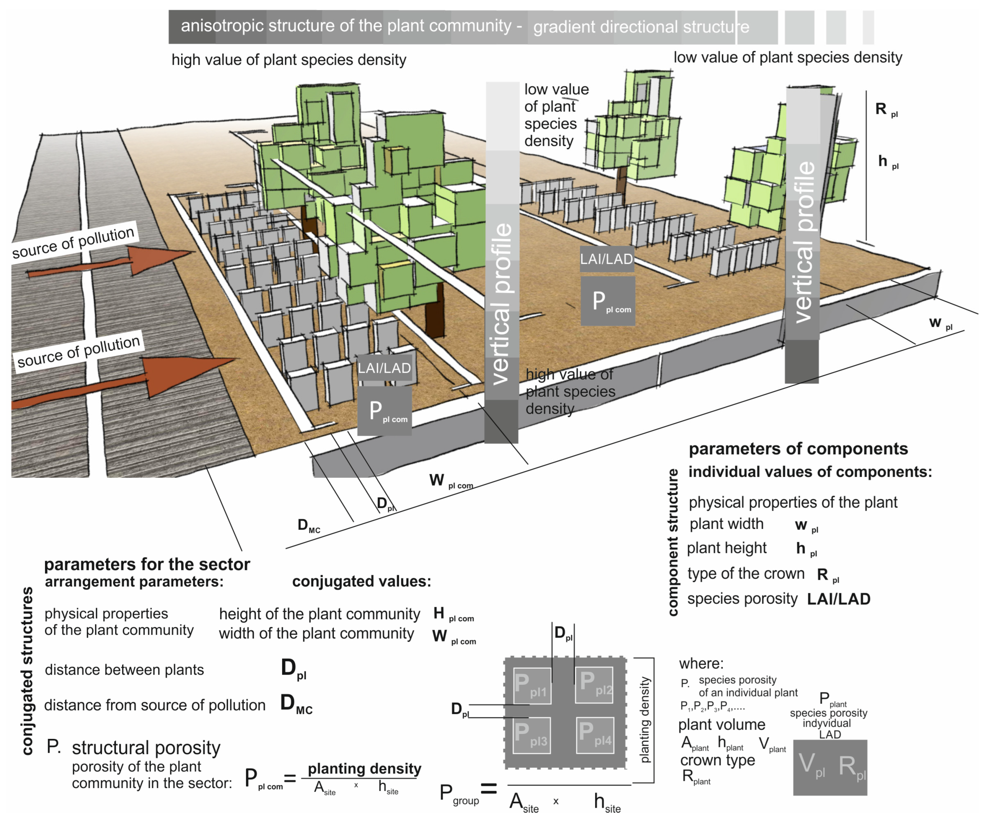
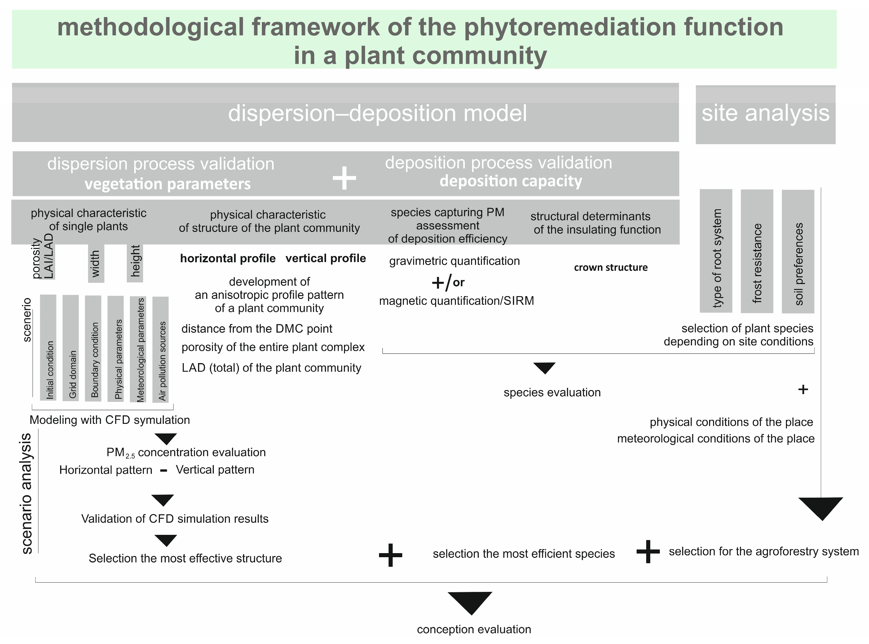
The optimization of the air phytoremediation process within the dispersion–deposition model is contingent on a synergistic methodology. This approach emphasizes the identification of correlated values and group parameters (Figure 1), considering environmental properties, individual plant characteristics, and spatial configurations that collectively influence the overall effectiveness of the formed group of plants [19,25].

Considering quality in a synergistic manner applies to both the deposition and dispersion processes. The deposition velocity (V_d) is a synchronous value which is the sum of the reciprocal of resistance (R_tot), which considers the aerodynamic resistance (R_a), boundary resistance (R_b), and canopy resistance (R_c) (Equation (3)) [19,25,26].

$${\mathrm{V}}_{\mathrm{d}}={\displaystyle \frac{1}{\mathrm{R}\mathrm{t}\mathrm{o}\mathrm{t}}}={\displaystyle \frac{1}{\mathrm{R}\mathrm{a}+\mathrm{R}\mathrm{b}+\mathrm{R}\mathrm{c}}}$$

(3)

where V_d—deposition velocity, R_tot—total resistance to deposition, R_a—aerodynamic resistance, R_b—boundary resistance, and R_c—canopy resistance.

By aggregating the partial attributes of individual elements, such as structural porosity indicated by LAI/LAD, as well as height, width, and the spatial configuration of plants relative to one another and the site (Distance to Maximum Concentration (DMC), site geometry), the comprehensive quality of the vegetation community is captured [19,22,25]. The values attributed to individual plants contribute to the collective values of conjugated parameters, thereby determining the quality of the plant group (Table 3).

Table 3. Plant characteristics, in terms of individual plants and groups, important for modelling the course of the dispersion process.

Plant Factors
At the Level of an Individual Plant (Individual Values of Plant)	At the Level of a Group of Plants: Parameters for the Sector-Arrangement Parameters and Conjugated Values
species deposition efficiency [g m−2] potential for shaping the value of porosity: filtration efficiency LAI [m2 m−2] insulating capacity LAD [m2 m−3] height [m] width [m] crown placement parameter [m]	distance from source of pollution/from the point DMC [m] Hplcom (height of the plant community)—parameter conjugated: the sum of the individual heights of low- and high-level plants (Equation (4)) Wplcom (width of the plant community)—parameter conjugated width of plants community (Equation (5)) Pplcom (barrier density–structural porosity)—the LAI/LAD value of individual plants, their sum in a plant community and the distribution of plants in each spatial unit (Equation (6), Figure 2 [41])

Table 3. Plant characteristics, in terms of individual plants and groups, important for modelling the course of the dispersion process.

Plant Factors
At the Level of an Individual Plant (Individual Values of Plant)	At the Level of a Group of Plants: Parameters for the Sector-Arrangement Parameters and Conjugated Values
species deposition efficiency [g m−2] potential for shaping the value of porosity: filtration efficiency LAI [m2 m−2] insulating capacity LAD [m2 m−3] height [m] width [m] crown placement parameter [m]	distance from source of pollution/from the point DMC [m] Hplcom (height of the plant community)—parameter conjugated: the sum of the individual heights of low- and high-level plants (Equation (4)) Wplcom (width of the plant community)—parameter conjugated width of plants community (Equation (5)) Pplcom (barrier density–structural porosity)—the LAI/LAD value of individual plants, their sum in a plant community and the distribution of plants in each spatial unit (Equation (6), Figure 2 [41])

While the height, width, and volume of plant structures can be easily summed up from individual elements (Equations (4) and (5)), the porosity of the entire plant group must consider the spatial context, including the population size (n) in a given spatial unit and the individual plant characteristics (R), and defining the nature of distribution by determining the rhythm of filling and gaps between plants (Equation (6); [41]). The characteristics of an individual plant contribute only partially to the overall porosity quality of the plant group, which is essentially built up by the arrangement parameters.

$${Hpl}_{com}={\sum }_1^{n}Hpl=h_1+h_2\dots +h_n [\mathrm{m}]$$

(4)

where ${\mathrm{H}\mathrm{p}\mathrm{l}}_{\mathrm{c}\mathrm{o}\mathrm{m}}$—total plant community height [m]; ${\mathrm{h}}_{\mathrm{i}}$—height of the i-th plant component [m]; $\mathrm{n}$—number of components.

$${Wpl}_{com}={\sum }_1^{n}Wpl=w_1+w_2\dots +w_n [\mathrm{m}]$$

(5)

where ${Wpl}_{com}$—total plant community width [m]; $w_i$—width of the i-th plant component [m]; $n$—number of components.

$${\mathrm{P}\mathrm{p}\mathrm{l}}_{\mathrm{c}\mathrm{o}\mathrm{m}}={\displaystyle \frac{1}{{\mathrm{A}}_{\mathrm{s}\mathrm{i}\mathrm{t}\mathrm{e}}\times {\mathrm{H}}_{\mathrm{s}\mathrm{i}\mathrm{t}\mathrm{e}}}}\sum _{\mathrm{s}+1}^{\mathrm{k}}\left({\mathrm{a}}_{\mathrm{s}}{\mathrm{H}}_{\mathrm{s}}{\mathrm{R}}_{\mathrm{s}}{n}_s\right)$$

(6)

where: ${\mathrm{P}\mathrm{p}\mathrm{l}}_{\mathrm{c}\mathrm{o}\mathrm{m}}$—plant community porosity index [-]; $A_{site}$—site area [m²]; $H_{site}$—site height [m]; $a_s$—crown projection area [m²]; $H_s$—plant height [m]; $R_s$—crown structure coefficient [-]; $n_s$—number of plants [-]; $s$—species index; $k$—number of species.

The importance of contextual recognition beyond individual characteristics can be illustrated using the crown placement parameter height. This value does not individually determine the phytoremediation efficiency, but only its coupling with the parameters of other plants and their arrangement shapes the tightness of the entire system.

An essential collective aspect is the introduction of directional grading of porosity values within the vegetation polyculture, which shapes a directional anisotropic character of tightness in a plant group across both horizontal and vertical profiles. The porosity gradient, depending on the geometry of the pollution source, shapes the course of interaction between plants and the flow of pollutants, activating individual stages of the process in appropriate places, supporting the blocking and filtering of pollutants and creating a deposition field [21,41].

Enhancing the phytoremediation efficiency of a plant community by optimizing the properties of the entire structure, rather than focusing solely on individual plant quality, significantly improves the effectiveness of the planned phytoremediation functions. This approach is particularly advantageous when the selection of plant species, and consequently the selection of individual plant qualities, is constrained by practical or production considerations, as is often the case with the planned crops, where selection is guided by plant utility and not by their strict phytoremediation values (Table 2 and

Table 4. Summary assessment of the suitability of plant species to perform phytoremediation functions, along with the assessment of their deposition capacities (all parameters are given on a scale from 1 to 3, with 1 indicating a low grade, 2 indicating moderately positive, and 3 indicating maximum positive assessment). A1—SIRM, A2—deposition capacity, B1—crown structure, B2—filtration efficiency (assessment of structural suitability in terms of insulation), B3—LAI/LAD (based on ENVI-met assumption), B4—insulating capacity, and C1—phytoremediation usefulness. For ease of identification, the columns of assessment on a subjectively adopted scale (A2, B2, B4, and C1) are highlighted in bold.

Species	The Vertical Stratification	A1 [µA]	A2 [1,2,3]	B1	B2 [1,2,3]	B3 * [m2 m−2/ m2 m−3]	B4 [1,2,3]	C1 [A2 + B2 + B4]
Acer campestre	higher layer	22	2	dense	3	3.9/2.0	3	2/3/3
Prunus avium	higher layer	13	2	intermediate	2	4.2/1.7	2	2/2/2
Sorbus intermedia	higher layer	26	3	intermediate	2	1.7	2	3/2/1
Quercus petraea	higher layer	17	2	dense	3	5.2/2.0	3	2/3/3
Sambucus nigra	higher layer	12	1	intermediate	2	1.2/1.7	2	1/2/2
Tilia platyphyllos	higher layer	18	2	Intermediate/ dense	3	6.0/1.3	2	2/3/2
Cornus sanguinea	lower layer	9	1	intermediate	2	1.2/1.7	2	1/2/2
Corylus avellana	lower layer	17	2	Intermediate/ dense	3	2.5/1.7	2	2/3/2
Viburnum opulus	lower layer	23	3	sparse	1	1.2/1.0	1	3/1/1
Prunus spinosa	lower layer	12	1	dense	3	1.2/2.0	2	1/3/2
Crataegus monogyna	lower layer	11	1	intermediate	2	1.7	2	1/2/2
Rosa rugosa	lower layer	24	3	dense	3	1.2/3	3	3/3/3

: Deposition processes. : Efficiency of the insulating and filtration. : Cumulative assessment. * The average LAI values for tree and shrub species were derived from Muhammad et al. (2023) [49]. These values were compared with the data from the ENVI-met software (LAD values ranging from 0.1 m² m⁻³ to 3.5 m² m⁻³).

).

2.3. Evaluation of the Impact of Vegetation on the PM Dispersion Process Using CFD Simulation

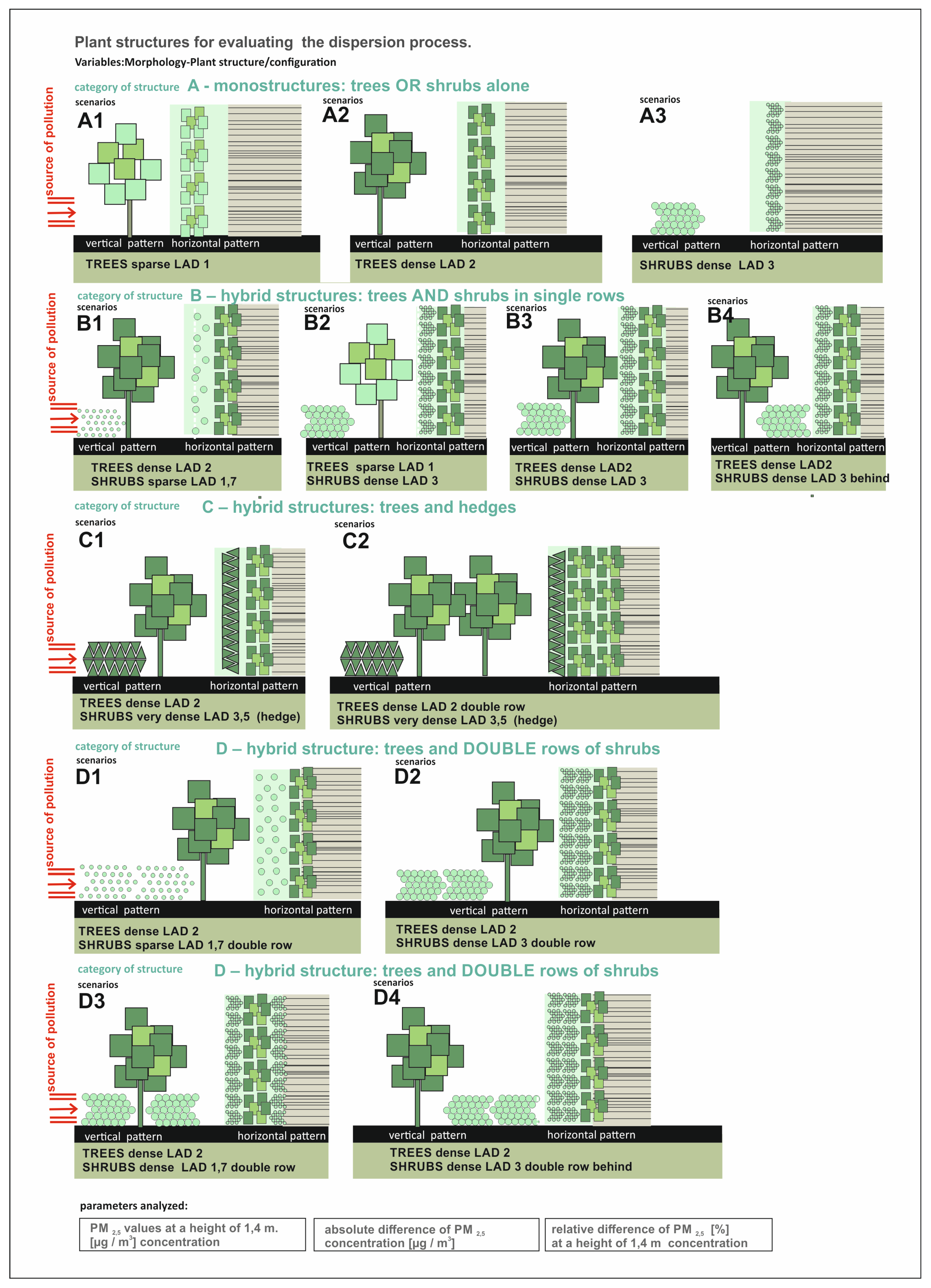
Phytoremediation performance in terms of dispersion processes was tested in several hypothetical situational scenarios, considering various spatial arrangements of plants shaping different parameter systems (Figure 3). The basic spatial structure adopted was a row arrangement of the arable system at a spacing of 50 m in the intercrop, where the first row was located 10 m from the pollution source (Figure 4). It should be explained that a typical linear road pollution pattern was assumed, where the source of pollution is located below the crown line. The distribution of PM_2.5 concentrations was observed in numerical experiments conducted using Micrometeorological Computational Fluid Dynamics models. These simulations were performed using ENVI-met software (Version: ENVI-met 5.6.1), a micro-climatological three-dimensional computational fluid dynamics model [53], widely recognized in air quality studies at the local scale [22,23,24,39,54]. In ENVI-met, particle transport is simulated using the Eulerian pollutant module in which concentrations evolve through advection and turbulent diffusion in the resolved flow field, while deposition is computed concurrently as a removal process. The model provides deposition-related outputs and represents dry deposition onto both built surfaces and vegetation; depending on the specified particle properties, gravitational settling may also contribute to particle removal [55]. Vegetation effects are represented primarily through canopy structure (e.g., the spatial distribution of canopy density/leaf area distribution), which is a common approach in vegetation–air quality modelling [23,40,56]. However, ENVI-met does not explicitly resolve species-specific leaves that are known to influence deposition velocities; such effects are typically parameterized in simplified ways in operational deposition modelling.

The simulations were conducted for a reference meteorological scenario with a perpendicular crosswind of 1 m s⁻¹. This setting was chosen as a conservative, high-impact case for near-road air quality because weak crosswinds reduce ventilation and promote pollutant accumulation while strengthening the interaction between the traffic plume and the roadside vegetation barrier. The numerical experiments illustrated horizontal and vertical patterns of PM_2.5 concentration resulting from the interaction of the pollution stream with various vegetation types. The simulation results showed the dependence of the effects on individual plant features and their configuration within the community, which allowed the identification of optimal systems under specific habitat conditions. Therefore, the results are interpreted as scenario-based and comparative across vegetation configurations.

2.4. Statistical Analysis

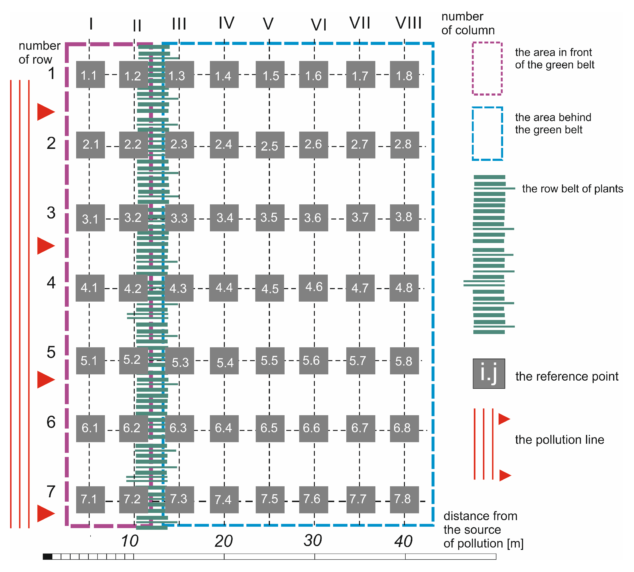
The results obtained from the numerical experiments were subjected to statistical analysis. The analysis of relative differences in PM_2.5 concentration for the five main scenarios (A, B, C, D, and the baseline scenario) allowed us to verify the efficiency of various selected plant arrangements for air purification purposes. The data were collected from the CFD simulation on the P × Q lattice given for the wind perpendicular to the direction of the pollution line and plant group. The PM_2.5 concentration was simulated in a column system, where the first column was located 5 m from the emission source (road), and the next seven rows of measurement points were introduced every 5 m, as shown in Figure 4. The arrangement contained 56 reference points placed in seven rows and eight columns. Two initial columns are supposed to be placed between the pollution source and the planned barrier.

The presentation of all collected data from the CFD simulation, specifically the pollution concentration at designated points, is conveniently structured in the form of a P × Q matrix (i = 1, …, P, j = 1, …, Q), where P = 7 represents the number of rows, and Q = 8 represents the number of columns. The superscripts 0, A, B, C, and D denote five primary scenarios. We conducted a statistical analysis of the data obtained from all reference points to ascertain the optimal plant arrangement. Furthermore, the data were deliberately divided into two subsets based on the natural division of the entire area into two zones: zone I, located between the emission source and the plant barrier (i = 1, …, 7; j = 1,2), and zone II, situated behind the barrier (i = 1, …, 7; j = 3, …, 8) (see Figure 4).

The effect of vegetation barriers on pollutant concentration is usually presented using the Average Relative Difference in Concentration (ARDC) summary parameter ${\delta }_{ARDC}$, which is one of the applicable air quality assessment indicators [22], calculated according to Equation (7):

$${\delta }_{ARDC}^{A(B,C,D)}= {\displaystyle \frac{1}{n}}{\sum }_{i, j}{\displaystyle \frac{C_{ij}^{A(B,C,D)}-C_{ij}^0}{C_{ij}^0}}$$

(7)

where $C_{ij}^0$ indicates the PM_2.5 concentration at the reference point in the baseline scenario, $C_{ij}^{A(B,C,D)}$ indicates the PM_2.5 concentration at the reference point after intervention (Scenario A, Scenario B, Scenario C, or Scenario D, respectively), and n indicates the number of reference points.

One may also determine the collective parameter of relative percentage change (RC) in total pollution concentration (Equation (8)), showing the difference in performance of specific vegetation.

$$RC={\displaystyle \frac{∆C^{A(B,C,D)}}{C^0}}$$

(8)

where

$$∆C^{A(B,C,D)}=C^{A(B,C,D)}-C^0$$

(9)

and

$$C^{A(B,C,D)}={\sum }_{i, j}{C}_{ij}^{A(B,C,D)}, C^0={\sum }_{i, j}{C}_{ij}^0$$

(10)

The last sum may be spread over various ranges of indices (i,j) depending on the context.

A one-way ANOVA was conducted to assess whether PM_2.5 concentration levels varied among the tested scenarios. Furthermore, post hoc analyses were performed using Tukey’s HSD test to evaluate differences among the scenarios. To enhance the analysis of the impact of the implemented green barriers, the second zone (located behind the barrier) was divided into two subsets: columns III–V (BI zone) and rows VI–VIII (BII zone). The first subset represents the area directly affected by traffic-related pollutants, where the implementation of green barriers resulted in a more substantial reduction in concentration. The second subset includes rows with very low concentration levels in the more remote sections of the analyzed area.

3. Results

3.1. Analysis of the Deposition Process—Performance of a Single Plant

The assessment of phytoremediation efficacy at the level of an individual plant was conducted through two primary approaches: firstly, by categorizing dry deposition potential based on data analysis (Table 4, values A1, A2), and secondly, by selecting appropriate characteristics of the plant’s crown to optimize filtration (B2) and insulation functions (B4) (Table 1 and Table 4).

The analysis conducted on 10 species, each representative of their use in AFS, revealed a deposition capacity ranging from 11 to 26 µA. This wide range, indicative of parameter variability, underscores the significant deposition capacity of plants employed in agroforestry practices [36]. A case-by-case analysis is imperative, particularly for species with uncertain potentials. An illustrative example is Viburnum opulus, which is recognized for its substantial deposition capacity but has a spreading, loose structure that results in excessively large gaps, even within a compact planting arrangement. Similar considerations apply to shrubs characterized by high compactness, where sparse planting can also result in permeable structures. These considerations led to the concept of coupled parameters, which are elaborated upon in the dispersion process (Section 2.1).

The analysis of the phytoremediation efficiency of species is presented in a clear tabular format (Table 2), addressing the key stages of the deposition process (deposition, filtration, isolation), defining the “property map” of the elements of the planned plant community (§2.1.3), and shaping the basis for the initial selection of species. The selection made, arranged in specific spatial settings and configurations, should then be verified to optimize dispersal processes.

3.2. Analysis of the Dispersal Process—Performance of the Phytoremediation in Terms of the Plant Community

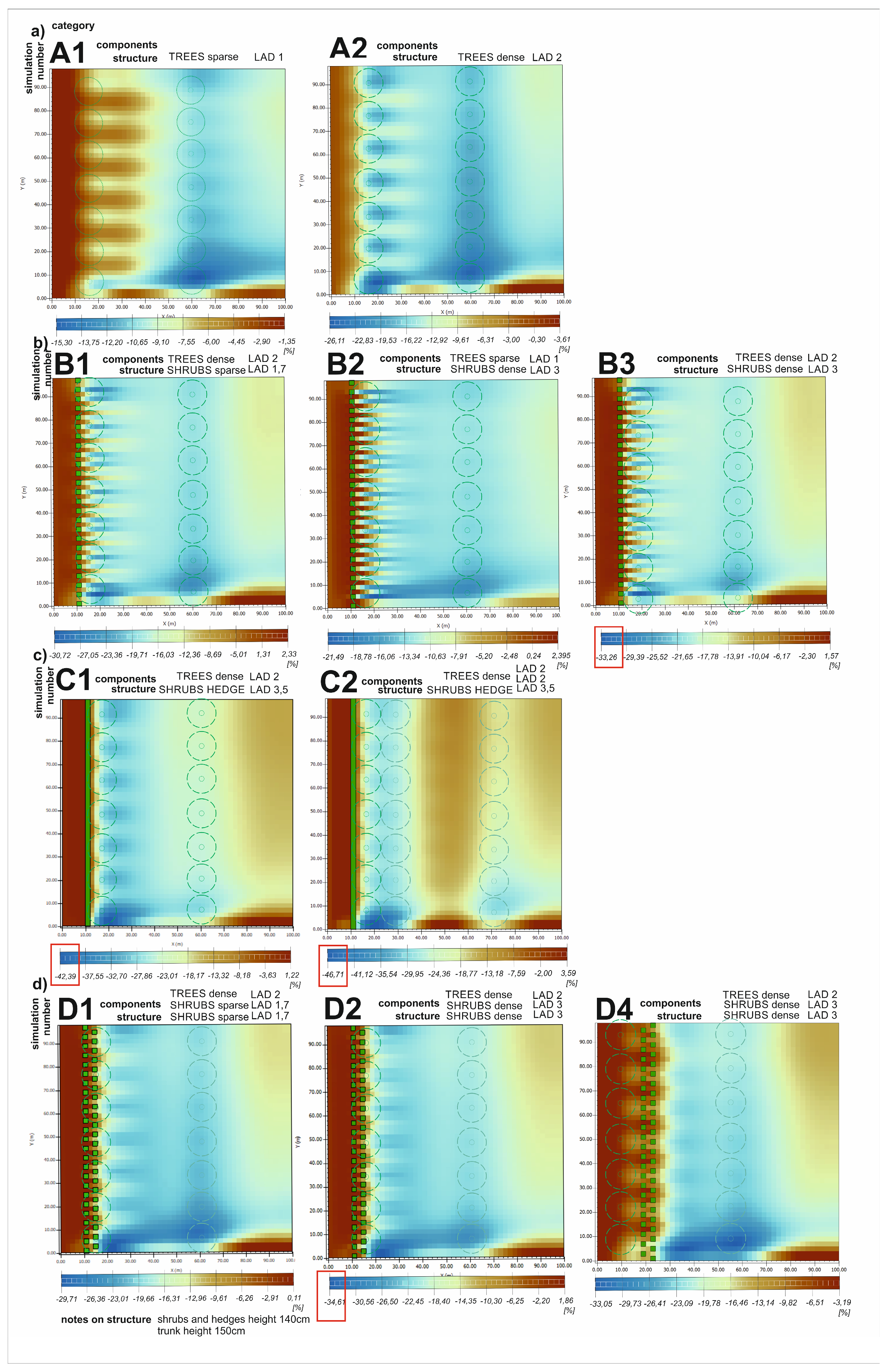
To assess the effectiveness of the dispersion processes, a two-stage analysis of PM_2.5 concentration variability was performed by shaping different arrangements of plant communities and thus manipulating their characteristics. Images of relative differences in PM_2.5 concentration [%] were compared (Figure 5, Figures S1 and S3 in Supplementary Materials), and statistical analysis was performed using data from readings from 56 measurement points at a height of 1.4 m (Table S3 in Supplementary Materials).

Analysis of the simulation images across categories A, B, C, and D revealed that the expansion of plant barriers in both the horizontal and vertical dimensions significantly enhanced phytoremediation effectiveness. The levels of concentration reduction achieved allowed for a clear categorization of the individual structures in terms of phytoremediation efficiency. Structures with a single layer of vegetation (category A) demonstrated the lowest efficiency, whereas those with expanded vertical and horizontal profiles, utilizing double lines of planted trees (C2) and shrubs (entire category D), exhibited the highest efficiency. Within each category, permutations of features were analyzed, providing insights into how the phytoremediation process can be intensified by specific components and their strategic arrangement.

Across all comparison groups, a direct correlation was observed between the density of the plant structure and the phytoremediation effect, illustrating the dependence of performance on the height of the LAD parameter both in terms of a single plant and a group of plants (Figure 5, Figures S1 and S3 in Supplementary Materials).

The correlation was validated for both the monostructures and hybrid structures. Monostructure systems (category A) exemplify this relationship with clarity, minimizing the impact of extraneous variables. In scenario A1 (low LAD of trees), the maximum reduction in PM_2.5 concentration reached up to 15% in certain areas, whereas in scenario A2 (high LAD of trees), the reduction exceeded 26% ((A1 vs. A2 scenario—Figure 5). These systems underscore the significance of individual species’ LAD parameters by examining plant strips with identical plant spacing, thanks to which the same structure is maintained, clearly displaying the effects. The analysis of hybrid multi-layer systems, which comprise combinations of trees and shrubs (groups B, C, and D), underscores the critical importance of adeptly managing the LAD parameter within the meaning of the collective LAD within vegetation groups. Comparative assessments revealed the superior efficacy of employing a higher LAD parameter, with maximum effectiveness observed in scenarios characterized by uniformly high LAD in medium- and high-level plants. This is particularly evident in configurations such as B3 and D2, which involve dense trees and dense shrubs arranged in single and double rows, respectively, as well as in category C, which utilizes hedges—notably, the highly efficient case of C2, which features a hedge and a double row of trees. Furthermore, the analysis of groups B, C, and D highlighted the significance of an appropriate LAD arrangement within individual sections, emphasizing the importance of the LAD parameter gradient pattern within the plant community, with scaling of the density values in the horizontal and vertical profiles, as demonstrated in cases B2 versus B1 and D2 versus D1 (Figure 5, Figures S2 and S3 in Supplementary Materials). It is worth noting, however, based on the comparison of various scenarios, including C1 vs. D2 and C2 vs. D2, it can be concluded that a large deposition field consisting of both loose (D1) and dense (D2) shrubs arranged in two rows is less effective than a narrower but compact hedge structure, providing a high level of isolation function. This suggests that for a linear pollution source, establishing a robust isolation function is the most effective strategy for reducing pollutant concentrations. These findings also corroborate the less pronounced but significant effects of other dense structures, such as B3/D1/D2.

The analysis of the modelling results enabled the identification of the most representative arrangements for subsequent statistical evaluation, focusing on the B3, D2, C2, and C1 scenarios.

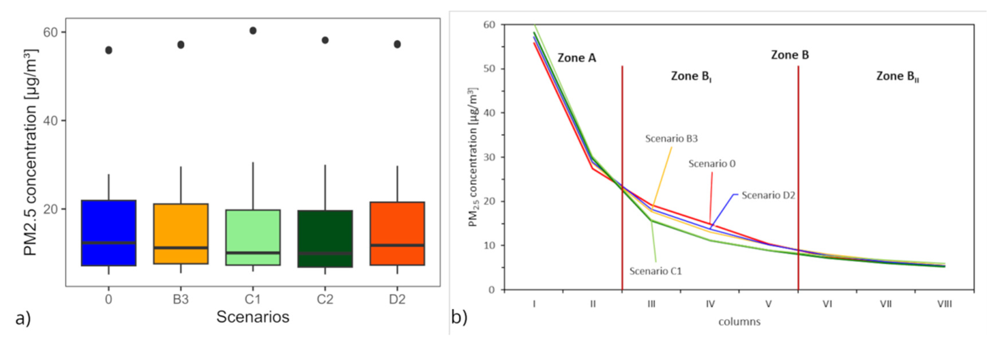
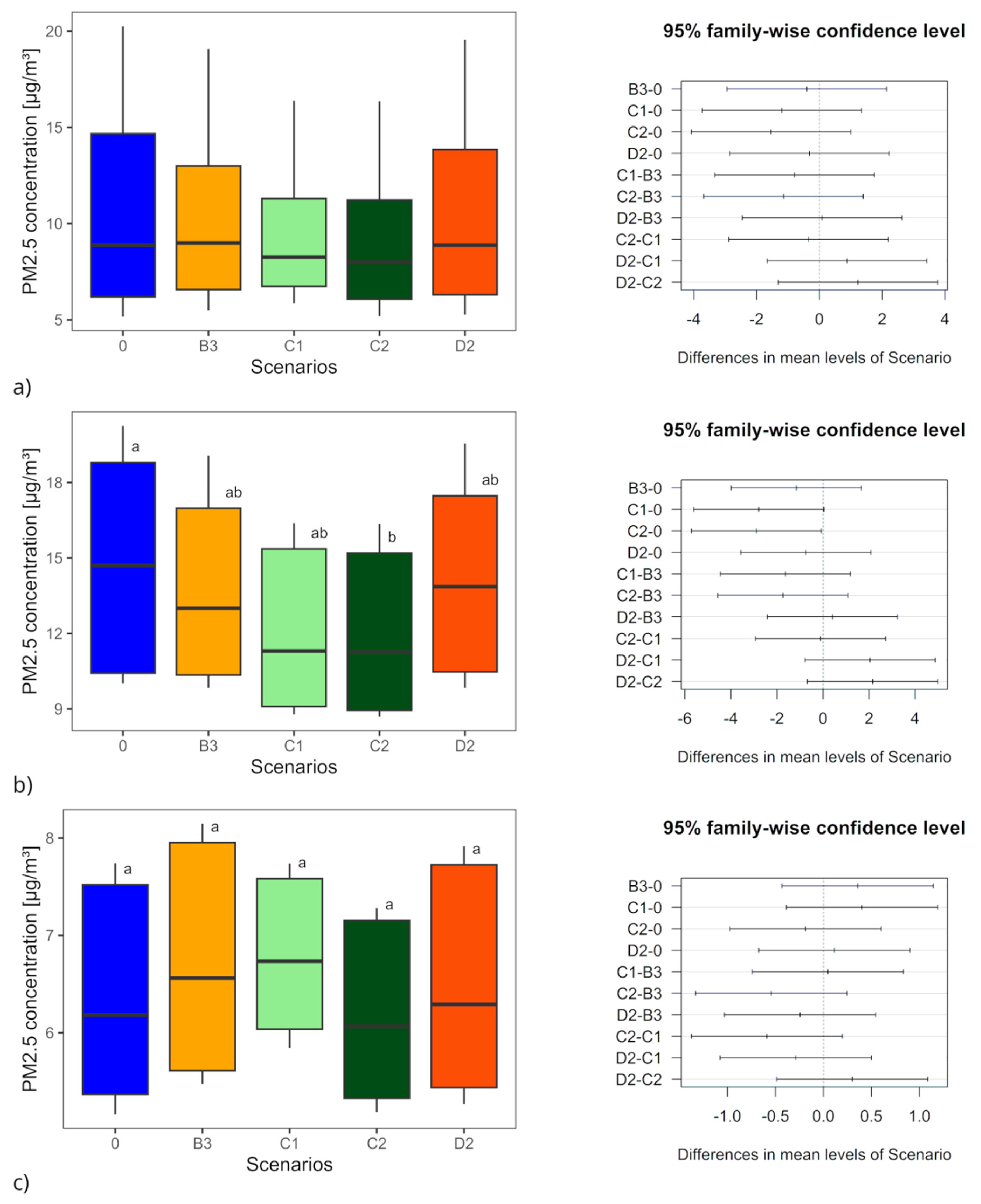
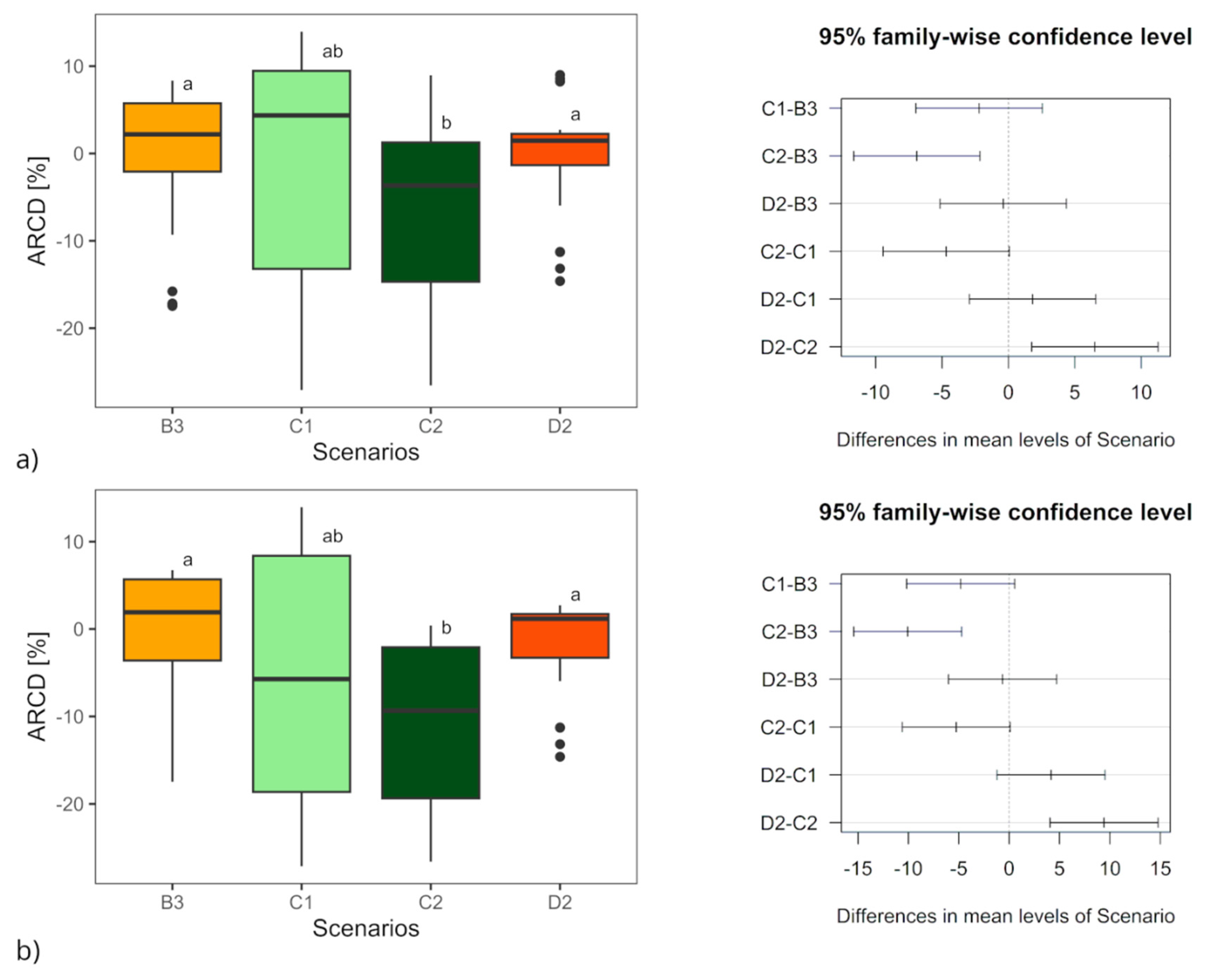
To conduct a comprehensive analysis of green barrier efficiency, it is essential to segment the area under investigation into distinct zones. The initial zone A represents the area situated in front of the green barrier, whereas zone B encompasses the area located behind the filtering barrier. Furthermore, zone B was subdivided into two subzones: BI, which included columns III–V and exhibited a pronounced influence of traffic-related emissions, and BII, where concentrations remained below 10 µg m⁻³ and displayed a uniform distribution. The most noteworthy aspect is the extent of PM_2.5 reduction in zone BI, as this metric serves as an indicator of the effectiveness of the implemented solution. Across the entire area under analysis, the PM_2.5 concentrations demonstrated a similar distribution (Figure 6). The one-way ANOVA revealed no statistically significant differences among the analyzed scenarios. The minimum PM_2.5 values recorded in the final columns ranged from approximately 5.2 µg m⁻³ (for scenarios 0 and C2) to 5.8 µg m⁻³ (for scenario C1), whereas the maximum values ranged from 57 µg m⁻³ (for the baseline scenario) to over 60 µg m⁻³ (for scenario C1). The median PM_2.5 concentration varied from approximately 10 µg m⁻³ (for scenarios C1 and C2) to 12.3 µg m⁻³ (for scenario 0). However, within the zone directly influenced by the green belt, a one-way ANOVA test indicated significant differences in PM_2.5 concentrations between scenario C2 and the baseline scenario (Figure 7). This finding highlights the superior phytoremediation efficiency of a configuration featuring a double row of trees and a dense hedge, characterized by a rich horizontal and vertical profile. In the scenario demonstrating maximum efficiency, the vegetation structure resulted in an approximate 14% reduction (RC parameter) in PM concentrations (scenario C2) within zone B (Figure 8,

Table 5. The average Relative Difference in Concentration (${\delta }_{ARDC}$) and RC values calculated from simulated data for the plant community between the analyzed scenario and the baseline scenario.

Parameter	Zone	B3	D2	C2	C1
${\delta }_{ARDC}$	The entire area	0.00	0.00	−0.07	−0.02
${\delta }_{ARDC}$	Zone A	0.04	0.04	0.06	0.09
${\delta }_{ARDC}$	Zone B	−0.01	−0.01	−0.11	−0.06
${\delta }_{ARDC}$	Zone BI	−0.07	−0.05	−0.19	−0.18
${\delta }_{ARDC}$	Zone BII	0.06	0.02	−0.03	0.07
RC [%}	The entire area	0.11	0.64	−3.21	0.08
RC [%}	Zone A	3.07	3.40	5.43	8.73
RC [%}	Zone B	−3.77	−2.98	−14.54	−11.26
RC [%}	Zone BI	−7.80	−5.03	−19.54	−18.82
RC [%}	Zone BII	5.60	1.79	−2.93	6.32

) and a more than 19% decrease in PM_2.5 concentration in Zone BI. Comparable results were observed for scenario C1, which comprised an arrangement of rows of trees and a dense hedge. To evaluate the statistical significance of the differences in ARDC values across various scenarios, a one-way ANOVA was conducted, followed by Tukey’s HSD test (Figure 8, Table 5). Statistically significant differences were identified between scenarios C2 and B3, as well as C2 and D2, when considering the entire area of analysis and specifically zone B. These findings corroborate the validity of the adopted categorization (A, B, C, and D) based on the complexity of the plant structure.

4. Discussion

The findings from the ENVI-met simulation revealed that strategically placing trees and shrubs, while considering the characteristics of each species and their individual structures, as well as spatial relationships within the community and in relation to the pollution source, can significantly enhance the phytoremediation effectiveness of row-alley agroforestry systems.

Optimizing the phytoremediation process involves considering the phase-based nature of the interaction between vegetation and the pollutant stream. The selection of plant parameters and the composition of plant communities, tailored to the individual phases, is responsible for achieving optimal efficiency of isolation, filtration, deposition, and dispersion. Statistical analysis of the most successful scenarios using the ARDC and RC parameters demonstrated a link between the efficiency of the phytoremediation process, the development of plant structure in horizontal and vertical profiles, and the distribution of parameters within these structures. This correlation supports the conclusions of earlier studies conducted through both numerical experiments and field research [21,23,25,31,55,56]. The initial step in structuring the plant community is to define the pollution source, including its geometry and location, which allows the direction and height of pollutant inflow to be determined in relation to low vegetation and tree crowns, and enables identification of the point of maximum concentration (DMC) [22].

The effective deposition of particles onto vegetation decreases with distance from the DMC, highlighting an important limitation of species-specific deposition potentials derived from laboratory experiments (Table 4, column A1). Under field conditions, deposition is jointly controlled by deposition velocity and local airborne concentration, commonly expressed as a deposition flux, F = V_dC. Therefore, even if V_d remains similar, a rapid decrease in concentration away from the source will lead to a pronounced decline in deposition flux with distance [57]. Consequently, the laboratory-derived ranking of species should be interpreted as deposition potential under controlled conditions, whereas actual field deposition will be reduced and strongly distance-dependent, especially for PM_2.5. Importantly, this supports the use of near-source deposition considerations in our study (Table 2, Table 4), because the first row of vegetation is located within ≤5 m of the source zone, where particle concentrations, and thus potential deposition flux, are expected to be highest [44,58]. The limited spatial reach of plant deposition potential highlights the importance of promoting heterogeneity in plant groups and expanding the profile [21,24], especially in near-source rows, thereby supporting a coherent recommendation for a multi-species polyculture system. A key finding concerns the crucial role of porosity, both as an individual plant trait and as a collective parameter of the plant community, corroborating the findings of previous studies [24,25,41,54]. The results obtained for category C (hedges with a single row, C1, and double-row lines, C2) surpassed those of the other configurations.

It has been shown that employing a stronger insulating barrier (with a high LAD) is more efficient than expanding the deposition field, and this approach is applicable to both single structures and double shrub barriers (as seen in the comparison between B3 and D1). At the same time, the variation in results obtained with different LAD values indicates that LAD is a strategic operational parameter and that its variability can significantly influence the phytoremediation efficiency of the plant community. In the present study, it is important to note that the Leaf Area Density (LAD) parameter is primarily considered as a collective parameter, and the high performance of category C is attributed to the tight structure of the entire group, specifically hedges and double rows of trees. This draws attention to the fact that, in addition to selecting an appropriate LAD assigned to a plant species, attention should be paid to parameters such as the height, width, and shape of individual crowns, as well as the height of the crown base. The arrangement and synchronization of these traits, together with species-specific LAD parameters, shape the collective compactness of the plant group, thereby creating a shared porosity value within each spatial area.

The significance of this factor is frequently highlighted in urban studies, where there is considerable variability in the efficiency of urban vegetation, which is influenced, among other factors, by planting density. In general, urban studies underscore the predominance of aerodynamic factors over deposition efficiency, noting that plantings, acting as obstacles, alter flow patterns [22,34,40]. This phenomenon can have both positive and negative implications and is strongly contingent upon other environmental conditions. In densely built urban environments, the implementation of vegetation that effectively obstructs ventilation presents significant limitations. Numerous studies have demonstrated that the introduction of vegetation in dense urban areas can lead to increased local pollutant concentrations [17,31,40,59]. Consequently, it is advisable to avoid dense rows of trees in street canyons and to employ vegetation with a limited impact on flow fields (e.g., single trees, low hedges) [25], which may appear contradictory to the recommendations presented in this article. However, the distinctly different morphological conditions of the areas under discussion should be considered. In urban settings, the introduction of a dense plant structure does not impede the inflow of pollutants as much as it obstructs the outflow, thereby limiting ventilation, preventing effective aerodynamic recirculation, and reducing dilution.

The necessity of proper vegetation configuration is confirmed in these studies, reinforcing the validity of multi-faceted analyses of implementation strategies.

Case C2 (Figure 5c(C2)) exemplifies a highly effective blocking barrier characterized by the implementation of very compact structures. However, despite its high effectiveness, an elevated concentration zone was observed between the rows, indicating pollutant accumulation, particularly in the vicinity of columns V–VIII, where other cases demonstrated a reduction in PM concentration. This case underscores that modifications in aerodynamic flow can also lead to a decrease in air-exchange rates and to alterations in vortex and turbulence patterns, potentially resulting in stagnation and localized increases in pollutant concentrations [40,59], analogous to the urban situations discussed above [25,40]. It is worth considering that focusing on a narrowly defined maximization approach may not lead to optimal efficiency at the general scale. A relevant reference is provided by Santiago (2017) [60], who reported that after planting, variability in average neighbourhood-scale concentration was small, while local differences in pollutant concentration exceeded 100%. These examples highlight the need to analyze the impact of tree cover on pollutant concentrations beyond basic quantification of the immediate surroundings. Urban studies emphasize the need to assess the effectiveness of tree cover (e.g., urban forests) at multiple scales, considering not only the immediate surroundings but also the broader context of the district or city. This phenomenon, known as the “green paradox”, reveals dramatically different impacts, with increased and decreased pollutant concentrations recorded for the same vegetation formation depending on the scale of analysis [40].

Moreover, attention should be paid to the specificity of planting in field areas, where there is no restrictive limitation on the area available for planting, as is often the case in cities.

It is worth noting that the satisfactory efficiency of the plant community with a looser but wider structure (category D, double rows of shrubs) indicates a trend that can be applied in certain practical circumstances. Although the highest concentration reductions were achieved with compact strips, the large deposition field was also effective. The advantage of this type of structure is that it exerts broader spatial influence and produces a more spatially uniform concentration reduction, demonstrating that phytoremediation efficiency can be improved not only by maximizing LAD. The effectiveness of a multi-layer structure in horizontal and vertical profiles, with substantial thickness providing an extended deposition area, may prove to be a useful alternative, especially when using certain crop species whose structure does not always meet the requirements for high LAD (see the case of Viburnum opulus in Section 3). Under certain conditions, a crown classified as intermediate may be preferable owing to the possibility of contamination penetrating deep into the crown, thereby providing a larger surface area for deposition. This aspect may be particularly important in plantings close to the pollution source, as discussed above.

The above analysis comprehensively covers issues related to the characteristics and configuration of plant structures with increased phytoremediation potential, providing a coherent picture of how this potential can be activated through manipulation of plant resources. A deliberate limitation of this work is the lack of analysis of effects under varying environmental conditions, leaving room for further research.

Phytoremediation, which is an ecological, cost-effective, and non-invasive method, belongs to the pool of passive, plant-related sustainable landscape practices [61]. It can be expected that implementing this function as an ongoing long-term process will provide more diverse and resilient agroforestry ecosystems, as indicated by researchers as beneficial [1,46,62], thereby guaranteeing the sustainable nature of such interventions [2,62] and providing an extension of the environmental affordances of agricultural systems in the area of atmospheric services [16,63,64].

5. Conclusions

Typical Agroforestry System (AFS) row-alley structures can be designed to enhance air phytoremediation processes, serving as an additional function alongside primary agricultural production.

Optimizing phytoremediation efficiency requires recognition of the quality at the level of individual plant properties, as well as their collective properties within a group in a specific area.

The selection of species with high deposition potential, the structure of individual plants, and the spatial arrangement within the plant community are strategic factors that determine the course of the individual stages of the phytoremediation process in terms of isolation, filtration, and deposition of pollutants.

It is recommended to create a multi-species plant polyculture in a layered arrangement with a complex horizontal and vertical profile and varying porosity values. The significance of porosity is highlighted in this context, both the porosity of a single plant and the porosity of a collective group of plants.

While the individual Leaf Area Density (LAD) value of plants is noteworthy, the manipulation of the compactness of the plant community structure is of paramount importance. Parameters such as height, width, stem height, and spacing between plants within a specified spatial unit are equally critical, as their configuration determines the porosity of the plant community.

In addition to obstructing pollutants, plant communities should also establish extensive areas for pollutant deposition and filtration. These areas should incorporate anisotropic structures with directional porosity gradation, both vertically and in terms of system depth.

References

1. Notaro, M.; Gary, C.; Le Coq, J.-F.; Metay, A.; Rapidel, B. How to increase the joint provision of ecosystem services by agricultural systems. Evidence from coffee-based agroforestry systems. Agric. Syst. 2022, 196, 103332. [Google Scholar] [CrossRef]
2. Veldkamp, E.; Schmidt, M.; Markwitz, C.; Beule, L.; Beuschel, R.; Biertümpfel, A.; Bischel, X.; Duan, X.; Gerjets, R.; Göbel, L.; et al. Multifunctionality of temperate alley-cropping agroforestry outperforms open cropland and grassland. Commun. Earth Environ. 2023, 4, 20. [Google Scholar] [CrossRef]
3. Estrada-Carmona, N.; Hart, A.K.; DeClerck, F.A.J.; Harvey, C.A.; Milder, J.C. Integrated landscape management for agriculture, rural livelihoods, and ecosystem conservation: An assessment of experience from Latin America and the Caribbean. Landsc. Urban Plan. 2014, 129, 1–11. [Google Scholar] [CrossRef]
4. Torralba, M.; Fagerholm, N.; Burgess, P.J.; Moreno, G.; Plieninger, T. Do European agroforestry systems enhance biodiversity and ecosystem services? A meta-analysis. Agric. Ecosyst. Environ. 2016, 230, 150–161. [Google Scholar] [CrossRef]
5. Montagnini, F.; Metzel, R. The Contribution of Agroforestry to Sustainable Development Goal 2: End Hunger, Achieve Food Security and Improved Nutrition, and Promote Sustainable Agriculture. In Integrating Landscapes: Agroforestry for Biodiversity Conservation and Food Sovereignty; Advances in Agroforestry; Springer International Publishing: Cham, Switzerland, 2017; pp. 11–45. [Google Scholar] [CrossRef]
6. Plieninger, T.; Muñoz-Rojas, J.; Buck, L.E.; Scherr, S.J. Agroforestry for sustainable landscape management. Sustain. Sci. 2020, 15, 1255–1266. [Google Scholar] [CrossRef]
7. Zomer, R.J.; Trabucco, A.; Coe, R.; Place, F.; van Noordwijk, M.; Xu, J.C. Trees on Farms: An Update and Reanalysis of Agroforestry’s Global Extent and Socio-Ecological Characteristics; World Agroforestry Centre (ICRAF): Nairobi, Kenya, 2014. [Google Scholar] [CrossRef]
8. Quandt, A.; Neufeldt, H.; Gorman, K. Climate change adaptation through agroforestry: Opportunities and gaps. Curr. Opin. Environ. Sustain. 2023, 60, 101244. [Google Scholar] [CrossRef]
9. Anderson, S.H.; Udawatta, R.P. Agroforestry: A system for improving soil health. In Agroforestry for Sustainable Agriculture; Burleigh Dodds Science Publishing: Cambridge, UK, 2019; pp. 317–334. [Google Scholar] [CrossRef]
10. Chen, B.; Lu, S.; Zhao, Y.; Li, S.; Yang, X.; Wang, B.; Zhang, H. Pollution Remediation by Urban Forests: PM2.5 Reduction in Beijing, China. Pol. J. Environ. Stud. 2016, 25, 1873–1881. [Google Scholar] [CrossRef]
11. Udawatta, R.P. Flood Control and Air Cleaning Regulatory Ecosystem Services of Agroforestry. In Agroforestry and Ecosystem Services; Springer International Publishing: Cham, Switzerland, 2021; pp. 305–330. [Google Scholar]
12. Rivest, D.; Lorente, M.; Olivier, A.; Messier, C. Soil biochemical properties and microbial resilience in agroforestry systems: Effects on wheat growth under controlled drought and flooding conditions. Sci. Total Environ. 2013, 463–464, 51–60. [Google Scholar] [CrossRef]
13. Biswas, B.; Chakraborty, D.; Timsina, J.; Bhowmick, U.R.; Dhara, P.K.; Lkn, D.K.G.; Sarkar, A.; Mondal, M.; Adhikary, S.; Kanthal, S.; et al. Agroforestry offers multiple ecosystem services in degraded lateritic soils. J. Clean. Prod. 2022, 365, 132768. [Google Scholar] [CrossRef]
14. Manes, F.; Marando, F.; Capotorti, G.; Blasi, C.; Salvatori, E.; Fusaro, L.; Ciancarella, L.; Mircea, M.; Marchetti, M.; Chirici, G.; et al. Regulating Ecosystem Services of forests in ten Italian Metropolitan Cities: Air quality improvement by PM10 and O3 removal. Ecol. Indic. 2016, 67, 425–440. [Google Scholar] [CrossRef]
15. Lin, C.H.; Weber, E.E.; Walter, W.D.; Lim, T.T.; Garrett, H.E.G. Vegetative Environmental Buffers for Air Quality Benefits. In North American Agroforestry; Garrett, H.E., Jose, S., Gold, M.A., Eds.; Wiley: Hoboken, NJ, USA, 2021. [Google Scholar] [CrossRef]
16. Prigioniero, A.; Postiglione, A.; Zuzolo, D.; Niinemets, Ü.; Tartaglia, M.; Scarano, P.; Mercurio, M.; Germinario, C.; Izzo, F.; Trifuoggi, M.; et al. Leaf surface functional traits influence particulate matter and polycyclic aromatic hydrocarbons air pollution mitigation: Insights from Mediterranean urban forests. J. Clean. Prod. 2023, 418, 138158. [Google Scholar] [CrossRef]
17. Chen, X.; Wang, X.; Wu, X.; Guo, J.; Zhou, Z. Influence of roadside vegetation barriers on air quality inside urban street canyons. Urban For. Urban Green. 2021, 63, 127219. [Google Scholar] [CrossRef]
18. Pandey, V.C.; Bajpai, O. Phytoremediation. In Phytomanagement of Polluted Sites; Elsevier: Amsterdam, The Netherlands, 2019; pp. 1–49. [Google Scholar]
19. Tiwary, A.; Williams, I. Air pollution control and mitigation. In Air Pollution, 4th ed.; CRC Press: Boca Raton, FL, USA, 2018; pp. 361–413. [Google Scholar]
20. Wei, X.; Lyu, S.; Yu, Y.; Wang, Z.; Liu, H.; Pan, D.; Chen, J. Phylloremediation of Air Pollutants: Exploiting the Potential of Plant Leaves and Leaf-Associated Microbes. Front. Plant Sci. 2017, 8, 1318. [Google Scholar] [CrossRef]
21. Vera, S.; Viecco, M.; Jorquera, H. Effects of biodiversity in green roofs and walls on the capture of fine particulate matter. Urban For. Urban Green. 2021, 63, 127229. [Google Scholar] [CrossRef]
22. Morakinyo, T.E.; Lam, Y.F.; Hao, S. Evaluating the role of green infrastructures on near-road pollutant dispersion and removal: Modelling and measurement. J. Environ. Manag. 2016, 182, 595–605. [Google Scholar] [CrossRef]
23. Heshani, A.L.S.; Winijkul, E. Numerical simulations of the effects of green infrastructure on PM2.5 dispersion in an urban park in Bangkok, Thailand. Heliyon 2022, 8, e10475. [Google Scholar] [CrossRef]
24. Baldauf, R. Roadside vegetation design characteristics that can improve local, near-road air quality. Transp. Res. Part D Transp. Environ. 2017, 52, 354–361. [Google Scholar] [CrossRef]
25. Janhäll, S. Review on urban vegetation and particle air pollution—Deposition and dispersion. Atmos. Environ. 2015, 105, 130–137. [Google Scholar] [CrossRef]
26. Buccolieri, R.; Jeanjean, A.P.R.; Gatto, E.; Leigh, R.J. The impact of trees on street ventilation, NOx and PM2.5 concentrations across heights in Marylebone Rd street canyon, central London. Sustain. Cities Soc. 2018, 41, 227–241. [Google Scholar] [CrossRef]
27. Beckett, K.P.; Freer-Smith, P.; Taylor, G. Effective Tree Species for Local Air quality Management. Arboric. Urban For 2000, 26, 12–19. [Google Scholar] [CrossRef]
28. Lee, B.X.Y.; Hadibarata, T.; Yuniarto, A. Phytoremediation Mechanisms in Air Pollution Control: A Review. Water Air Soil Pollut. 2020, 231, 437. [Google Scholar] [CrossRef]
29. Gong, C.; Xian, C.; Wu, T.; Liu, J.; Ouyang, Z. Role of urban vegetation in air phytoremediation: Differences between scientific research and environmental management perspectives. npj Urban Sustain. 2023, 3, 24. [Google Scholar] [CrossRef]
30. Mori, J.; Hanslin, H.M.; Burchi, G.; Sæbø, A. Particulate matter and element accumulation on coniferous trees at different distances from a highway. Urban For. Urban Green. 2015, 14, 170–177. [Google Scholar] [CrossRef]
31. Jeanjean, A.P.R.; Monks, P.S.; Leigh, R.J. Modelling the effectiveness of urban trees and grass on PM2.5 reduction via dispersion and deposition at a city scale. Atmos. Environ. 2016, 147, 1–10. [Google Scholar] [CrossRef]
32. Kafle, A.; Timilsina, A.; Gautam, A.; Adhikari, K.; Bhattarai, A.; Aryal, N. Phytoremediation: Mechanisms, plant selection and enhancement by natural and synthetic agents. Environ. Adv. 2022, 8, 100203. [Google Scholar] [CrossRef]
33. Chen, J.; Hoek, G. Long-term exposure to PM and all-cause and cause-specific mortality: A systematic review and meta-analysis. Environ. Int. 2020, 143, 105974. [Google Scholar] [CrossRef]
34. Abhijith, K.V.; Kumar, P. Quantifying particulate matter reduction and their deposition on the leaves of green infrastructure. Environ. Pollut. 2020, 265, 114884. [Google Scholar] [CrossRef]
35. Dzierżanowski, K.; Popek, R.; Gawrońska, H.; Sæbø, A.; Gawroński, S.W. Deposition of Particulate Matter of Different Size Fractions on Leaf Surfaces and in Waxes of Urban Forest Species. Int. J. Phytoremediat. 2011, 13, 1037–1046. [Google Scholar] [CrossRef]
36. Sæbø, A.; Popek, R.; Nawrot, B.; Hanslin, H.M.; Gawronska, H.; Gawronski, S.W. Plant species differences in particulate matter accumulation on leaf surfaces. Sci. Total Environ. 2012, 427–428, 347–354. [Google Scholar] [CrossRef]
37. Muhammad, S.; Wuyts, K.; Samson, R. Atmospheric net particle accumulation on 96 plant species with contrasting morphological and anatomical leaf characteristics in a common garden experiment. Atmos. Environ. 2019, 202, 328–344. [Google Scholar] [CrossRef]
38. Sgrigna, G.; Baldacchini, C.; Esposito, R.; Calandrelli, R.; Tiwary, A.; Calfapietra, C. Characterization of leaf-level particulate matter for an industrial city using electron microscopy and X-ray microanalysis. Sci. Total Environ. 2016, 548–549, 91–99. [Google Scholar] [CrossRef]
39. Barwise, Y.; Kumar, P. Designing vegetation barriers for urban air pollution abatement: A practical review for appropriate plant species selection. npj Clim. Atmos. Sci. 2020, 3, 12. [Google Scholar] [CrossRef]
40. Vos, P.E.J.; Maiheu, B.; Vankerkom, J.; Janssen, S. Improving local air quality in cities: To tree or not to tree? Environ. Pollut. 2013, 183, 113–122. [Google Scholar] [CrossRef]
41. Podhajska, E.; Halarewicz, A.A.; Zienowicz, M.; Deszcz, R.; Podhajski, B. Structural and parametric aspects of plant barriers as a passive method for improving urban air quality. City Environ. Interact. 2020, 8, 100048. [Google Scholar] [CrossRef]
42. Du, M.; Zhao, Y.; Yang, J.; Wang, W.; Luo, X.; Zhong, Z.; Huang, B. Impact of ENVI-met-Based Road Greening Design on Thermal Comfort and PM2.5 Concentration in Hot–Humid Areas. Sustainability 2024, 16, 8475. [Google Scholar] [CrossRef]
43. Meng, F.; Wu, Y.; Ma, D.; Yang, B.; Diao, H.; Dong, D.; Zhang, J.; Jin, X.; Jin, X.J.; Chen, J.; et al. Environmental justice at a crossroads: Examining the impact of vegetation and building patterns on road-sourced PM2.5 dispersion and population exposure. Ecol. Front. 2025, 45, 667–677. [Google Scholar] [CrossRef]
44. Xing, Y.; Brimblecombe, P. Urban park layout and exposure to traffic-derived air pollutants. Landsc. Urban Plan. 2020, 194, 103682. [Google Scholar] [CrossRef]
45. Elbakidze, M.; Surová, D.; Muñoz-Rojas, J.; Persson, J.-O.; Dawson, L.; Plieninger, T.; Pinto-Correia, T. Perceived benefits from agroforestry landscapes across North-Eastern Europe: What matters and for whom? Landsc. Urban Plan. 2021, 209, 104044. [Google Scholar] [CrossRef]
46. Andreotti, F.; Mao, Z.; Jagoret, P.; Speelman, E.N.; Gary, C.; Saj, S. Exploring management strategies to enhance the provision of ecosystem services in complex smallholder agroforestry systems. Ecol. Indic. 2018, 94, 257–265. [Google Scholar] [CrossRef]
47. Viñals, E.; Maneja, R.; Rufí-Salís, M.; Martí, M.; Puy, N. Reviewing social-ecological resilience for agroforestry systems under climate change conditions. Sci. Total Environ. 2023, 869, 161763. [Google Scholar] [CrossRef]
48. Ghezehei, S.B.; Annandale, J.G.; Everson, C.S. Modelling radiation interception and water balance in agroforestry systems. In Tree-Crop Interactions: Agroforestry in a Changing Climate; CABI: Wallingford, UK, 2015; pp. 41–56. [Google Scholar] [CrossRef]
49. Deepika; Haritash, A.K. Phytoremediation potential of ornamental plants for heavy metal removal from contaminated soil: A critical review. Hortic. Environ. Biotechnol. 2023, 64, 709–734. [Google Scholar] [CrossRef]
50. Karg, J. Zadrzewienie Śródpolne, Strefy Buforowe i Miedze; Ministerstwo Rolnictwa i Rozwoju Wsi: Warszawa, Poland, 2003.
51. Finnigan, J. Turbulence in Plant Canopies. Annu. Rev. Fluid Mech. 2000, 32, 519–571. [Google Scholar] [CrossRef]
52. Russavage, E.; Thiele, J.; Lumbsden-Pinto, J.; Schwager, K.; Green, T.; Dovciak, M. Characterizing Canopy Openness in Open Forests: Spherical Densiometer and Canopy Photography Are Equivalent but Less Sensitive than Direct Measurements of Solar Radiation. J. For. 2020, 119, 130–140. [Google Scholar] [CrossRef]
53. Bruse, M. Modelling and strategies for improved urban climate and air quality. In Proceedings of the 6th International Conference on Urban Climate, Gothenburg, Sweden, 12–16 June 2006; International Association for Urban Climate (IAUC): Dublin, Ireland, 2011. [Google Scholar]
54. Buccolieri, R.; Santiago, J.-L.; Rivas, E.; Sanchez, B. Review on urban tree modelling in CFD simulations: Aerodynamic, deposition and thermal effects. Urban For. Urban Green. 2018, 31, 212–220. [Google Scholar] [CrossRef]
55. Deng, S.; Ma, J.; Zhang, L.; Jia, Z.; Ma, L. Microclimate simulation and model optimization of the effect of roadway green space on atmospheric particulate matter. Environ. Pollut. 2019, 246, 932–944. [Google Scholar] [CrossRef]
56. Abhijith, K.V.; Kumar, P. Field investigations for evaluating green infrastructure effects on air quality in open-road conditions. Atmos. Environ. 2019, 201, 132–147. [Google Scholar] [CrossRef]
57. Zhu, D.; Kuhns, H.D.; Gillies, J.A.; Etyemezian, V.; Gertler, A.W.; Brown, S. Inferring deposition velocities from changes in aerosol size distributions downwind of a roadway. Atmos. Environ. 2011, 45, 957–966. [Google Scholar] [CrossRef]
58. Gao, Z.; Cizdziel, J.V.; Wontor, K.; Clisham, C.; Focia, K.; Rausch, J.; Jaramillo-Vogel, D. On airborne tire wear particles along roads with different traffic characteristics using passive sampling and optical microscopy, single particle SEM/EDX, and µ-ATR-FTIR analyses. Front. Environ. Sci. 2022, 10, 1022697. [Google Scholar] [CrossRef]
59. Setälä, H.; Viippola, V.; Rantalainen, A.-L.; Pennanen, A.; Yli-Pelkonen, V. Does urban vegetation mitigate air pollution in northern conditions? Environ. Pollut. 2013, 183, 104–112. [Google Scholar] [CrossRef]
60. Santiago, J.-L.; Martilli, A.; Martin, F. On Dry Deposition Modelling of Atmospheric Pollutants on Vegetation at the Microscale: Application to the Impact of Street Vegetation on Air Quality. Bound. Layer Meteorol. 2016, 162, 451–474. [Google Scholar] [CrossRef]
61. Hajipour, S.; Alinia-Ahandani, E.; Behnaz, S.-B.; Zahra, A.-T.; Selamoglu, Z.; Akram, M. Phytoremediation potential and its methods—A review. Bioeng. Stud. 2023, 4, 1–8. [Google Scholar] [CrossRef]
62. Zanzi, A.; Andreotti, F.; Vaglia, V.; Alali, S.; Orlando, F.; Bocchi, S. Forecasting Agroforestry Ecosystem Services Provision in Urban Regeneration Projects: Experiences and Perspectives from Milan. Sustainability 2021, 13, 2434. [Google Scholar] [CrossRef]
63. Elagib, N.A.; Al-Saidi, M. Balancing the benefits from the water–energy–land–food nexus through agroforestry in the Sahel. Sci. Total Environ. 2020, 742, 140509. [Google Scholar] [CrossRef] [PubMed]
64. van Noordwijk, M.; Speelman, E.; Hofstede, G.J.; Farida, A.; Abdurrahim, A.Y.; Miccolis, A.; Hakim, A.L.; Wamucii, C.N.; Lagneaux, E.; Andreotti, F.; et al. Sustainable Agroforestry Landscape Management: Changing the Game. Land 2020, 9, 243. [Google Scholar] [CrossRef]
Figure 1. Stages of programming the air phytoremediation function in a plant community, considering the aspects of dispersion and deposition, as well as aspects of species selection and site conditions.
Forests 17 00405 g001
Figure 2. Formation of conjugated structural porosity of the plant community (Pgroup)—description and development of the structural image of a given plant community in each spatial unit parameterizes the porosity of the structure, considering the population size (n) of a given species and individual plant characteristics (R). P1 (…)—individual LAD values for individual plants; P group—the porosity of the entire unit; Vpl—the volumetric capacity of the elements (1,2,3); A1—the area of the plant crown projection area (species number 1, LAI1); h1—the height of the plant (species number 1); R1—the crown typology indicator; (species number 1)—defining the structure of the crown, specific for a given species; Asite—the area of the entire unit; Hsite—the height of the entire unit; n—typology indicator: the all population of a given species in given areas; and k—species ordinal number.
Forests 17 00405 g002
Figure 3. The structural scenarios for the first row were as follows: Scenario 0, no isolation row of plants; Scenario A, monostructures: trees alone or shrubs alone; Scenario B, hybrid structures: trees and shrubs in single rows; Scenario C, hybrid structures: trees and hedges, single and double rows, respectively; and Scenario D, hybrid structures: double rows of shrubs plus trees. In the scenarios, two LAD values were developed: sparse and dense structures. The input data for the simulations are presented in Supplementary Materials (Table S1).
Forests 17 00405 g003
Figure 4. The 56-reference-point matrix of vegetation barriers allows for the area to be analyzed in horizontal rows (1–7) and vertical columns (I–VIII). The diagram indicates the distribution of the matrix (i.j) adopted for statistical analysis.
Forests 17 00405 g004
Figure 5. The compilation and analysis of the most characteristic scenarios for the arrangement of plant communities: (a) Scenario A1/Scenario A2/Scenario A3—comparison of monostructured arrangements using low LAD trees versus high LAD trees; (b) Scenario B1/Scenario B2/Scenario B3—comparison of hybrid structured arrangements; (c) Scenario C1/Scenario C2/Scenario D2—comparison of the performance of strictly structured (hedge) and double-row rows; (d) Scenario D1/Scenario D2/Scenario D4—analysis of the importance of the location and quality of low-layer plants. The juxtaposition illustrates the gradual increase in system performance relative to the introduction of an increasing LAD value and the effect of rearranging the row of shrubs forming the low layer of the plant barrier.
Forests 17 00405 g005
Figure 6. The concentrations were compared by dividing the study area into distinct zones and comparing the results. The average PM2.5 concentration values (a) and the effectiveness of green barriers (b) were analyzed with a distinction between zones A and B in vertical sections (columns I–VIII), illustrating PM concentration changes at specific distances from the emission source (rows 1–8) using various vegetation structure variants (Scenario 0, B3, C1, C2, and D2). The graph displays values from all columns, with points representing the average values from these columns. Based on the assumptions, the critical area for phytoremediation was identified as zone B, situated beyond the green belt, with a further distinction of subzone BI, the area directly influenced by the green barrier.
Forests 17 00405 g006
Figure 7. Diagrams for PM2.5 mass concentrations simulated for different green belt scenarios and different zones and Tukey’s HSD test analysis: (a) zone B, (b) zone BI, (c) zone BII. Letters above boxplots indicate Tukey’s HSD grouping; boxplots sharing the same letter are not significantly different.
Forests 17 00405 g007
Figure 8. ARDC value [%] for the whole area (a) and for zone B (b). Letters above boxplots indicate Tukey’s HSD grouping; boxplots sharing the same letter are not significantly different.
Forests 17 00405 g008