


Abstract
Spanning structures that must be maintained, not merely rebuilt, underlie sensor fabrics, peer-to-peer overlays, and software-defined networks. We give a complete treatment of distributed minimum-spanning-tree (MST) construction and maintenance built on non-tree-edge (NTE) tracking, which certifies the edges excluded from the tree rather than growing tree fragments. First, we provide the full specification and correctness proofs of the static NTE algorithm—previously available only in outline—achieving messages of bits in rounds with only three message types. Second, we prove an exact maintenance algorithm for edge-weight updates: three of four update cases resolve in , and the fourth is resolved by ExactSwap within a message bound that experiments show to be tight (median ratio 1.00); across 221,874 update records, the median affected set is 2, independent of scale (–). Third, we establish a separation result: verifying a replacement edge distributively provably requires examining the entire search region, an obstruction with no centralized analogue. Fourth, we show that prediction is best used for scheduling: under contention, prioritizing predicted-cheap updates improves mean time-to-resolution by 2.1–3.8× over FIFO, matching an oracle, with a linear model sufficing.
1. Introduction
The infrastructures that define large-scale computing today are wide-area, fully distributed, and in constant flux. Sensor fabrics in the Internet of Things coordinate thousands of energy-constrained nodes whose links degrade and whose members die [1,2]; peer-to-peer and overlay networks reorganize continually under churn [3]; federated-learning deployments train models across participant sets that grow and shrink between rounds [4,5]; and software-defined fabrics must repair multicast and control structures when links fail [6]. All of these depend on a common substrate: a low-cost spanning structure over the current participants. Building that structure once is a solved problem; keeping it correct and minimal as the infrastructure changes—without re-running a global computation on every event—is not, and at the scales above, the difference between rebuilding and repairing is the difference between an infrastructure that spends its bandwidth and energy on its mission and one that spends them on self-maintenance.
Distributed construction of a minimum spanning tree (MST), the canonical such structure, is a classical problem in distributed computing, with algorithms dating to Gallager, Humblet and Spira (GHS) [7] and a substantial line of subsequent work improving message and time complexity [8,9,10,11,12]. Almost all of this work addresses static construction: given a fixed graph, build its MST once. In practice, the networks these algorithms run over rarely stay fixed. Peer-to-peer overlays experience churn as participants join and leave; wireless sensor networks lose nodes to battery depletion and suffer channel-quality fluctuation from interference and mobility; software-defined network fabrics reprovision links and route around failures. An MST built once becomes stale as soon as the underlying graph changes, and the naive response, recomputing from scratch, discards everything the network already knew and pays the full construction cost again.
How often this matters is an empirical question, and the answer shapes what a dynamic algorithm should optimize for. Real link costs change on two very different timescales, and only discrete structural events—not short-term measurement jitter—alter the optimal tree; our update model makes this distinction explicit and grounds it in measurement literature.
The applications motivating this distinction are concrete and, in two cases, the author’s own prior work. Ragab and Haque [13] applied an early, structurally-outlined version of the algorithm formalized in full here to eliminate duplicate packet delivery in -bounded multicast overlay clusters for peer-to-peer video streaming—an application where peer churn and link-quality fluctuation are the norm. Khan and Haque [14] applied MST-based aggregation to extend the lifetime of power-limited sensor networks, where node death from battery depletion is a discrete event of exactly the kind our dynamic extension is built to handle efficiently—a motivation independently echoed by the Dynamic GHS of Díaz et al. [15]. Beyond these, the same structure recurs in SDN-controlled multicast tree maintenance under link failure, in decentralized federated learning’s communication-efficient client overlays under participant churn, and, as very recent work confirms [16], in large-scale dynamic graph analytics generally, where full MST recomputation is explicitly noted to lack practical efficiency under frequent updates.
Learning-augmented algorithms offer a further tool for problems of this shape. Lykouris and Vassilvitskii [17] and subsequent work [18] give online algorithms access to a machine-learned prediction, with guarantees that improve when the prediction is accurate and degrade no worse than a prediction-free baseline when it is not. Van den Brand et al. [19] extend this framework to dynamic graph algorithms (reachability, shortest paths, matching) in a centralized model. Whether an analogous guarantee is available for distributed MST maintenance is a natural question we investigate; the answer, established in Section 5.5, is more nuanced than a straightforward “yes.”
Against this background, our contributions are as follows. First, a full specification and correctness proof of the NTE (non-tree-edge tracking) distributed MST algorithm (Section 4), first outlined in the author’s earlier conference paper [13] and originating in the author’s dissertation [20]. The conference presentation established the two-phase structure, the module decomposition and message types, and proofs of Path Optimality and graph orientation, but stated the complexity without proof; we supply the complete module-level specification (full slate design and per-module pseudocode), the Cycle Theorem, Theorem NTE with its supporting lemmas, and the complexity proofs.
Second, a provably correct, non-learned algorithm for maintaining the MST under a sequence of edge-weight changes (Section 5), achieving rounds and messages, summed over the smaller side of the induced cut, for the one update case that can force a structural change—a bound tightened, via a structural observation about spanning-tree cuts, well below the naive degree-based estimate.
Third, a separation between the distributed and centralized settings (Section 5.5, Proposition 4): in the distributed model, verifying the true minimum-weight replacement edge provably requires examining the full search region—no distance-based local certificate can confirm a partial search using only information visible within a bounded region. This obstruction has no analogue in centralized dynamic-MST maintenance, where global visibility makes the question moot. It cleanly delimits what any distributed algorithm, learned or not, can achieve for this problem, and directly motivates the design of our fourth contribution.
Fourth, a scheduling-aware use of prediction built on top of the proven algorithm (Section 6): since the true replacement edge cannot be found via a shortcut, prediction instead informs when the unavoidable computation is carried out, letting systems that tolerate bounded staleness prioritize cheap and small updates over expensive ones without ever affecting correctness (Proposition 5).
The remainder of the paper is organized as follows. Section 2 surveys related work; Section 3 defines the model; Section 4 gives the static algorithm; Section 5 the dynamic extension and the separation result; Section 6 the scheduling layer; Section 7 the experimental evaluation; and Section 9 concludes.
2. Related Work
2.1. Classical Distributed MST
The foundational result is Gallager, Humblet and Spira’s distributed MST algorithm [7], which grows fragments and merges them by a minimum-outgoing-edge rule, achieving time and messages; Chin and Ting [21] improved its time to almost linear. Awerbuch [8] improved the time to , optimal with respect to n, retaining near-linear message complexity; Garay, Kutten and Peleg [9] then argued that the network diameter is the more sensitive parameter and gave the first diameter-sensitive sublinear-time algorithm, running in rounds (throughout, d denotes the network diameter; see Section 3). Faloutsos and Molle [10] revisited these algorithms and clarified correctness subtleties. Lotker, Patt-Shamir, Pavlov and Peleg [11] gave an -round algorithm for fully connected (overlay-style) networks. All of these are tree-edge-tracking: non-tree edges are discarded once superseded. The present paper inverts this, tracking the non-tree edges via the Path Optimality criterion (Theorem 2); the approach was outlined in the author’s conference paper [13] and is specified and proved in full here.
2.2. Modern CONGEST-Model MST
The CONGEST model [22] is the standard cost model for network-scale distributed algorithms: nodes compute in synchronous rounds and each link carries at most bits per round, so bandwidth, not local computation, is the scarce resource, matching the economics of the infrastructures in Section 1 (Section 3 gives the formal definition). Within it, Kutten and Peleg [23] achieved rounds, near-optimal in view of the lower bound of Peleg and Rubinovich [24], which holds even for networks of diameter ; Pandurangan, Robinson and Scquizzato [12] attained near-optimality in both rounds and messages simultaneously, and Elkin [25] gave a simple deterministic algorithm with near-optimal time and message complexity; Khan and Pandurangan [26] gave fast distributed approximation algorithms. Parallel (as opposed to message-passing distributed) constructions form a neighbouring line (e.g., Huang’s fully pipelined MST constructor [27]) analyzed under parallel cost models rather than the CONGEST message/round accounting used here. These results target worst-case round complexity as the primary metric, in contrast to this paper’s emphasis on simplicity of message structure: three message types and six modules.
2.3. Dynamic MST: Centralized Settings
A separate line maintains an MST under updates in a centralized model with full access to the graph in memory. Sleator and Tarjan’s dynamic trees [28] underlie much of it (alongside Karger, Klein and Tarjan’s randomized linear-time static construction [29]); Frederickson [30] gave the first -per-update structures; Eppstein, Galil, Italiano and Nissenzweig’s sparsification [31] improved this generically; Holm, de Lichtenberg and Thorup [32] gave the first polylogarithmic fully-dynamic algorithm, and Eppstein et al. [33] handled the planar case. A related sub-problem (maintaining a replacement for every tree edge simultaneously) culminates in a recent engineered solution [16]. Recent engineering work continues the centralized line: Luo et al. [34] update an MST under batches of edge and vertex changes by reusing the surviving portion of the previous tree and continuing Kruskal’s algorithm from it, motivated explicitly by backbone maintenance in ad hoc IoT networks—again presuming full in-memory access to the graph. This centralized line differs from ours in two ways worth making explicit. First, what is maintained: the replacement-maintenance approach [16] eagerly maintains a replacement for every tree edge (affordable on a single machine) whereas our ExactSwap (Section 5) computes a replacement reactively. Second, and more fundamentally, what “local information” means: a centralized algorithm can determine the true global minimum crossing edge directly, whereas a distributed algorithm cannot in general certify that a partial search has found the true minimum without examining a provably sufficient region (Section 5.5, Proposition 4)—an obstruction with no analogue in the centralized setting.
2.4. Dynamic MST: Sensor Networks and Distributed Settings
Awerbuch, Cidon and Kutten [35] studied optimal maintenance of a (not necessarily minimum) spanning tree under topology change, establishing the classical distributed-maintenance baseline; the present paper maintains the minimum spanning tree specifically. Díaz et al. [15] proposed a distributed dynamic GHS (DGHS) for wireless sensor networks, motivated by GHS’s lack of tolerance to change: node failures and time-varying channel quality require the tree to be repaired rather than rebuilt, since rebuilding costs sensor nodes scarce battery energy. This motivation is essentially our own for Section 5, applied to a different base algorithm; DGHS does not address the CONGEST complexity questions our Claims 4–6 resolve, nor does it include a learning-augmented layer. A further distributed-maintenance line is the self-stabilizing one: Gupta and Srimani’s self-stabilizing multicast protocols for ad hoc networks [36] maintain a spanning structure that recovers from arbitrary transient faults, an objective adjacent to but stronger than ours. Two lines address exactly this setting—a fixed communication topology whose edge weights change. Peleg [37] gave a distributed correction algorithm for minimum-weight spanning trees after weight changes, which stores the full tree at each node. Foerster et al. [38] formalize the batch dynamic CONGEST model, in which a batch of weight changes arrives at once, and maintain an MST in rounds with only bits of auxiliary state per node, together with an lower bound that is tight up to a polylogarithmic factor in . Their accounting is per batch, in rounds and space, and their algorithm broadcasts the changed labels network-wide to compute a matroid basis; ours is per single update, in messages, and confines work to the affected region, whose size we measure directly (Section 7). The two are complementary: for a single change their round bound is , comparable to ours, but the message cost of a global broadcast is incurred regardless of how localized the actual repair is.
2.5. Learning-Augmented Algorithms
Lykouris and Vassilvitskii [17] introduced the modern framework; Purohit, Svitkina and Kumar [39] established its consistency–robustness tradeoffs for scheduling problems, and Mitzenmacher and Vassilvitskii [18] survey the area. Van den Brand et al. [19] extend it to dynamic graph algorithms (reachability, shortest paths, matching) in a centralized setting, with predictions concerning the timing of future updates. Their work addresses neither MST nor the distributed CONGEST model. We investigate whether their framework extends to distributed MST; the answer is instructive rather than straightforwardly positive—Section 5.5 shows that the partial-search verification their mechanisms would require has no sound distributed analogue for this problem. Section 6 accordingly repositions the learning-augmented contribution around scheduling decisions that do not require certifying a shortcut’s correctness.
2.6. Adjacent Distributed P2P and Overlay Tree Constructions
The most directly comparable work is that of Abdel-Wahab et al. [40]: a fully distributed MST algorithm for wide-area communication networks, motivated, like ours, by efficient multicast. It grows disjoint trees concurrently, each repeatedly joining its closest neighbouring tree, until a single tree remains; the construction is fragment-growing in the GHS lineage and addresses the static problem only. The author’s prior work [13] applies the NTE static construction within -bounded MON-Clusters for P2P video streaming. Hossain and Khan’s ZePoP [41] elects a delay-optimal leader by closeness centrality and builds a data collection and distribution tree rooted at it, optimizing delay rather than edge-weight minimality; a centrality-based construction and an MST-based one solve genuinely different problems, and their outputs need not coincide. Mokhtarian and Jacobsen [42] address minimum-delay overlay multicast, a distinct objective. At the infrastructure level, structure-placement and lifetime-optimization problems—load-balanced gateway placement in wireless mesh backbones [43], lifetime optimization of dense sensor deployments [2], and aggregation-point placement for semi-decentralized federated learning [44]—optimize related objectives at coarser granularity; the present work supplies the tree-maintenance primitive that such infrastructure-level optimizers implicitly assume.
3. Model and Preliminaries
3.1. Graph Model
Let be a connected, undirected graph with nodes and edges, where assigns a positive weight to each edge. We write d for the diameter and for the maximum degree. As is standard in CONGEST, edge weights are assumed polynomial in n, so a weight fits in bits.
Assumption 1
(Unique weights). All edge weights are distinct. This is without loss of generality: ties break by the pair , ordered lexicographically: iff , or and . This total order is used wherever edge weights are compared—in the orientation rule (Section 4.3) and in every candidate comparison of the detection and maintenance phases. Uniqueness makes the MST unique. In practice, quantized or coarsely reported link metrics produce many exact ties; the identifier tie-break then decides deterministically, correctness is unaffected, and the only consequence of near-equal weights is that a different—equally valid—minimum spanning tree may be selected.
Definition 1
(MST; tree and non-tree edges). The minimum spanning tree is the acyclic edge subset connecting all of V with minimum total weight. Edges in T are tree edges, and edges in are non-tree edges (NTEs). For an NTE , its fundamental cycle is the cycle formed by and the unique tree path between u and v; the tree edges on that path are the edges the cycle crosses.
3.2. Distributed Computation Model
We work in the synchronous CONGEST model [22]. A processor resides at each node; computation proceeds in synchronous rounds; each round, every node sends one message of at most bits across each incident edge. Links are bidirectional and reliable. Each node initially knows its own -bit identifier, its neighbors’ identifiers, and its incident edge weights. Cost is measured in total messages (one message across one link = one unit) and rounds. At least one node, the session initiator, is awake at the start and designates an update initiator.
3.3. Slate State
Each node maintains local state called its slate, specified in Section 4. Two fields on which the dynamic extension depends on:
Definition 2
(Subtree size). With the tree rooted per the orientation of Section 4, is the number of nodes in the subtree rooted at v, maintained as a byproduct of reply-aggregation at no additional asymptotic cost.
Definition 3
(Candidate weight). For each NTE e recorded in a node’s slate, the field stores the maximum tree-edge weight on e’s fundamental cycle as of the last refresh. The field is populated by a post-construction labeling pass (Section 4)—not from the comparison value observed at detection time, which provably differs from the fundamental-cycle maximum in general (Remark 1)—and thereafter maintained by affected-set refresh. It is what makes the stability check of Lemma 1 possible.
3.4. Dynamic Update Model
Definition 4
(Update sequence). An update sequence is , where each changes the weight of one existing edge to , preserving uniqueness (Assumption 1). Edge insertions and deletions, and hence node arrival and departure, are outside this model and are deferred to future work; Section 5.4 shows how each case reduces to the machinery developed here. Updates are observed initially only by the endpoints of , and are well-separated in time. Simultaneous or bursty changes are handled by serialization: concurrent updates enter a queue and are processed one session at a time, which is exactly the contended regime evaluated in Section 7 (a stream of 4000 updates under a fixed per-round budget), where scheduling order becomes the performance lever.
Real link costs exhibit two kinds of variation on very different timescales, a distinction long established by Internet measurement studies. The first is short-timescale jitter: delay fluctuation from queuing and contention, small relative to the weight gaps between distinct edges. Such fluctuation does not change the relative order of edge weights, and therefore cannot change the MST, by Assumption 1 and Path Optimality (Theorem 2). Measurement studies support this: path properties such as round-trip time are operationally steady over the intervals that matter here [45]. Discrete structural events—route changes, point-of-presence reassignment, link re-provisioning—occur on the scale of minutes to weeks [46] and do change the optimal tree. Only the latter are modeled as elements of ; node failure, which removes a vertex rather than re-weighting an edge, is the topology-change case deferred above: a practical implementation applies a hysteresis threshold so that jitter never triggers processing, and the well-separated-updates assumption is realistic under this reading, since the per-update processing cost of Section 5 is far below typical inter-arrival times of structurally meaningful changes. The same two-timescale structure holds in wireless sensor networks, where link quality drifts with interference and mobility while re-routing and transmission-power adjustment shift link costs abruptly; node death from battery depletion is again the deferred topology-change case. After each is processed, the invariant holds, with each node’s slate current.
4. The Static NTE Algorithm
This section gives the full specification, correctness proofs, and complexity of the NTE-tracking algorithm, introduced in outline in [13] and originating in [20]. The conference presentation established the two-phase structure, the module decomposition, and proofs of Path Optimality and graph orientation, but stated complexity without proof; we supply the full module-level specification and slate design, the Cycle Theorem, Theorem NTE, and the complexity proofs.
4.1. Overview
The algorithm’s central design choice is to identify the non-tree edges—the set whose membership has a strictly local certificate (Path Optimality, Theorem 2)—rather than growing tree fragments. It runs in two phases: an orientation phase converting the undirected graph into an acyclic directed graph via request and reply messages, and an NTE detection phase in which update messages flow from the update initiator back toward the session initiator, each NTE identified by exactly one node en route. Six modules generate and aggregate the three message types.
4.2. Messages and Slate Variables
Each node’s slate is initialized with , the sentinel value meaning unleveled; levels are assigned by the request flood of the orientation phase (Section 4.3), empty parent, child, and NTE sets, and zeroed aggregation fields. Three message types are used. A request carries six fields (sender/receiver id, sender level, session-initiator id, update-initiator id, session id); a reply carries three (sender/receiver id, ACK/NACK); an update carries six (sender/receiver id, candidate-edge, max-link, non-shared-candidate-edge, max-link-non-shared-path). All fields are bits (Claim 1).
Each node’s slate holds its id, neighbor set, incident edge costs, level, parent/child sets, the request sets , and the working fields , , the detected-NTE set, and (Definition 3).
Remark 1
(The aggregation runner-up is not the fundamental-cycle maximum). At the moment a node detects an NTE by comparing two branch max-links, the runner-up value is the maximum weight along the alternative aggregation path back to the update initiator—which may traverse non-tree edges and omit tree edges of the NTE’s fundamental cycle. In Figure 1 graph, simulation shows that the runner-up diverges from the fundamental-cycle maximum on four of the six NTEs, in both directions. Divergence either way is unsafe for the check of Lemma 1: a too-high value triggers spurious swaps, a too-low one silently misses required swaps. The runner-up therefore must not be used as .
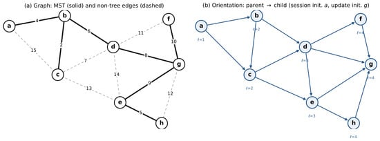
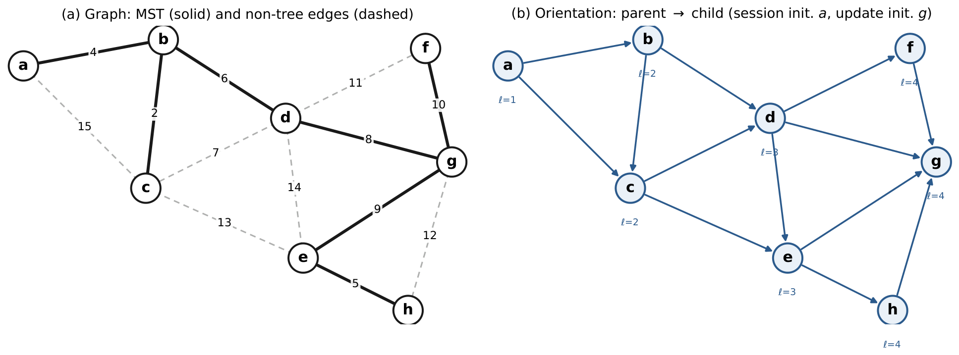
Figure 1.
The worked-example graph of Section 4.5. (a) The weighted graph with MST edges solid and non-tree edges dashed. (b) The oriented DAG produced by the orientation phase, with levels ℓ and parent→child arcs; session initiator a, update initiator g.
The field is instead populated by a post-construction labeling pass over the final tree, assigning each node a label supporting maximum-edge-weight queries on tree paths (in the Korman–Kutten line of distributed MST-verification labeling [47], whose label size is optimal, with W the largest edge weight; under the polynomial-weight convention of Section 3 this is bits), after which each NTE’s endpoints compute the fundamental-cycle maximum from their labels. The pass is required only for the dynamic extension; a static-only deployment may omit it.
4.3. Graph Orientation
For node v, let be its identifier, its neighbors, and the nodes from which it received a request. The level function assigns each node the position at which it first received a request; we write as a sentinel value denoting that v has not yet been leveled:
The third case is transient: it describes a node the request wave has not yet reached, and it is precisely the state tested by the request aggregator’s opening guard (Section 4.4), which enforces the first-request rule. Since G is connected and requests flood to all neighbors, every node is leveled within rounds (see Claim 3), so f is total over V at termination and the sentinel never survives to the end of the orientation phase. The slate initializes (Section 4.2), matching this sentinel convention. Each edge is oriented so that is the parent of when
Levels are assigned once per update session by the request flood and remain fixed for the remainder of that session; the orientation of Equation (2) is therefore static throughout the detection phase, and changes only when a new session re-floods.
Orienting the edges of a graph by a vertex numbering, so that every edge points from lower to higher number, is a standard way to obtain an acyclic orientation [48]. The rule below instantiates this idea with a numbering the protocol can compute in one flood—levels first, identifiers as tie-breakers—plus an override that makes the update initiator the unique sink; the statement records the properties this specific rule guarantees.
Theorem 1
(Graph Orientation). A directed graph is acyclic if and only if its nodes can be numbered such that, for every arc , .
Proof.
(⇒) Suppose a cycle exists on with arcs , , . If , arcs force , so , contradicting , which, by (2) requires . If , the tie-break forces , again contradicting closure. If , then contradicts . (⇐) Symmetric case analysis on level/id ordering. □
Orientation guarantees that the detection phase propagates without deadlock: every message flows from a lower level to a higher one. Levels are assigned by breadth-first arrival, so a node adjacent to two differently-leveled nodes takes the smaller-level parent’s level plus one.
4.4. The Six Modules
The algorithm uses six event-driven modules: request generator, request aggregator/propagator, reply aggregator, update generator, update aggregator, and the degenerate-case handler. Pseudocode is given in Appendix A; the update aggregator, the heart of the detection phase, appears as Algorithm 1.
| Algorithm 1 Update Aggregator (at internal node s) |
|
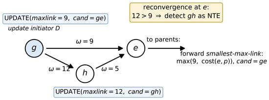
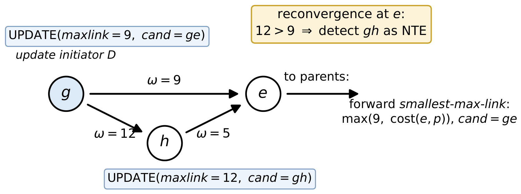
The aggregation step, in words (Figure 2). The update phase is a wave that starts at the update initiator D (the unique childless node of the orientation) and flows child-to-parent toward the session initiator. Every Update message carries two values: max-link, the largest edge cost on the path the wave has traversed from D to the sender, and candidate-edge, the identity of the edge attaining it. A node with a single child merely extends the path: it forwards the pair, raising max-link if its own outgoing edge is heavier (line 13). Detection happens where the wave reconverges: when a node s has received from two (or more) children, the two branch paths from D to s together close a cycle—this is the situation of Proposition 1—and the heaviest edge on that cycle is simply the larger of the two branch max-links (line 6). By Proposition 2 that edge cannot belong to the MST, so s records it as an NTE (line 7). The smaller max-link—the runner-up—describes the surviving path from D to s and is what continues upward (line 12), again raised by as the wave proceeds (line 14). Figure 2 traces one such meeting; ties between branch maxima are broken by the non-shared-path comparison of lines 8–10, which consults only the portions of the two paths beyond their last common node.
Figure 2.
The aggregation step on the worked example of Figure 1 (update initiator ). Two branch paths reconverge at e: the child g reports and the child h reports . The larger max-link identifies its candidate edge as a non-tree edge (Proposition 2); the runner-up pair (the pseudocode’s smallest-max-link) is forwarded to e’s parents, raised by the outgoing edge cost (Algorithm 1, line 13). Exactly one cycle is closed per reconvergence, which is the content of Proposition 1.
4.5. Worked Example
Consider Figure 1 with weights , , , , , , , , , , , , ; session initiator a, update initiator g. Independent recomputation gives tree edges (weight 44) and NTEs . A full simulation of the oriented-DAG aggregation reproduces exactly six detections— at e, and at d, at c, at b, at a—matching the independently computed NTE set.
4.6. Correctness
The following characterization is classical: it is equivalent to the cut and cycle properties of minimum spanning trees [48,49] (see also the Path Optimality conditions of network-flow theory). We state it in the form the protocol exploits and include the one-paragraph proof for self-containment; a proof also appears in the conference paper [13].
Theorem 2
(Path Optimality). A spanning tree is an MST if and only if, for every non-tree edge , for every edge on the -path between k and l.
Proof.
(⇒) If on the path had , swapping for gives a lighter spanning tree, contradicting minimality. (⇐) If the inequality holds throughout, no single-edge swap decreases total weight, and since any spanning tree reaches any other by such swaps, is minimum. □
Proposition 1
(Cycle Theorem). If two paths converge at a node during the detection phase, exactly one cycle—and hence exactly one non-tree edge—is produced.
Proof.
Let aggregation occur at s with update initiator u. Paths share an initial segment to some k, then diverge through distinct (distinct because if , node q would already have detected the cycle and forwarded one path), reconverging at s. Then is a single cycle, introducing exactly one chord. □
Proposition 2.
The edge of maximum cost among the two paths aggregated at a node is a non-tree edge.
Proof.
Immediate from Theorem 2 and Proposition 1: the heaviest edge on the unique cycle cannot lie in any MST containing the cycle’s other edges. □
Theorem 3
(Theorem NTE). Let be the NTEs detected at node i. Then .
Proof.
Via three lemmas. (i) is a spanning tree. Every node retains exactly one surviving path to the update initiator D (the update aggregator keeps only the smaller-max-link branch), so the result is connected, spans V, and is acyclic. (ii) Each detected is genuinely a non-tree edge of G. Detection at v via candidate implies (Proposition 2); any alternative k–l path through another node u has all edges lighter still, so by Path Optimality remains non-tree. (iii) No NTE remains undetected. By (i) the result is already a tree with edges; removing more would disconnect it. Combining (i)–(iii) with Theorem 2 and Proposition 1 gives the claim. □
4.7. Complexity
Claim 1
(Message size). Every message is bits.
Proof.
Identifiers are bits; the level is bounded by n. Each message carries a constant number of such fields. □
Claim 2
(Message complexity). The algorithm uses messages.
Proof.
At most requests (one per incident edge per side, plus at most one conflict resolution), replies, and m updates (one per oriented parent-child pair): at most total. □
Claim 3
(Time complexity). The algorithm completes in rounds.
Proof.
Request propagation from session to update initiator is ; replies proceed concurrently; update propagation back is . □
Table 1 compares against prior algorithms. The NTE advantage is not asymptotically better message complexity than the best modern CONGEST results, but a smaller message-type count and simpler per-message structure—properties that matter for the dynamic extension, where each message type’s role in affected-set maintenance must be tracked explicitly. When the dynamic extension is deployed, the labeling pass adds its own cost (a distributed maximum-weight-on-tree-path scheme in the Korman–Kutten line [47]) as a separate line item; a static-only deployment does not incur it.
Table 1.
Comparison with prior distributed MST algorithms. Here d is the network diameter (Section 3); hides polylogarithmic factors. † Randomized (Las Vegas); all other entries, including ours, are deterministic. GKP analyze time only and do not bound message complexity.
5. Dynamic NTE-MST Framework
This section presents a correct, complete, non-learned algorithm for maintaining the MST under edge-weight updates, built on Section 4. Section 6 builds a scheduling layer on top; nothing there is required for this section’s claims.
5.1. Case Analysis
An update falls into exactly one of four cases:
- Case A (non-tree edge, weight increases): e remains non-tree by Path Optimality. Cost , no messages.
- Case B (non-tree edge, weight decreases): decided in by Lemma 1; if a swap results, the leaving edge is known from the slate—no search.
- Case C (tree edge, weight decreases): e remains a tree edge. Cost .
- Case D (tree edge, weight increases): the one case that can force a structural change; resolved by ExactSwap (Section 5.2).
Lemma 1
(Stability Verification, Case B). Let be a non-tree edge, and let denote its stored value: the maximum tree-edge weight on its fundamental cycle (Definition 3). On update : if , then remains non-tree, verifiable in by one local comparison; if , then enters the tree and the edge achieving leaves it—a swap whose leaving edge is already identified by the endpoint labels (Section 4.2), so that, in contrast to Case D, no search is required: the splice and the slate refresh reuse ExactSwap ’s update machinery while skipping its search phase entirely.
Proof.
Immediate from Path Optimality (Theorem 2): stays non-tree exactly when its weight is not less than the heaviest tree edge on its fundamental cycle, which is . The comparison needs no messages since is local slate state. □
Case B can therefore change the tree’s edge set; what distinguishes it from Case D is not the absence of structural change but the absence of discovery. In Case B the entering edge is the updated edge itself and the leaving edge is determined by the state the endpoints already hold; in Case D the replacement must be found, and Proposition 4 shows that finding it provably requires searching the full region. “Three of four cases resolve in ” refers to this decision cost.
5.2. The Affected Set and the ExactSwap Protocol
Let Case D occur at tree edge , p the parent of c. Removing e splits the tree into (rooted at c) and .
Definition 5
(Affected set). The affected set of a Case-D update at e is the set of non-tree edges whose fundamental cycle crosses e—equivalently, those with exactly one endpoint in . These are exactly the NTEs whose becomes stale when e leaves the tree.
The protocol ExactSwap: (1) since both know , let be the smaller of (); (2) the root of floods a one-bit marker to its members; (3) each marked node probes its non-tree incident edges for cut-crossing candidates; (4) a convergecast reports the minimum-weight crossing edge; (5) if lighter than , it replaces e, and affected slates update by piggyback on steps 3–4.
Step 3’s restriction to non-tree edges rests on a structural fact: within a spanning tree, every edge crossing the cut induced by removing e, other than e itself, is necessarily a non-tree edge—so tree-edge neighbors need not be probed.
5.3. Complexity of ExactSwap
Claim 4
(Messages). ExactSwap resolves a Case-D update in messages, the sum over , where is v’s non-tree degree.
Proof.
Steps 2 and 4 cost each; step 3, by the structural fact above, probes only non-tree incident edges, costing , which dominates. □
Claim 5
(Rounds). ExactSwap resolves a Case-D update in rounds, which is at most .
Claim 6
(Message size). All ExactSwap messages are bits.
The message bound of Claim 4 is empirically 9– of the naive degree-based bound , with the largest improvement on scale-free graphs (Section 7).
5.4. Beyond Weight Updates: Insertions, Deletions, Departures
The update model of Section 3 covers weight changes to existing edges; the machinery above nonetheless already decides the natural extensions. For insertion:
Proposition 3
(Insertion decision). Let a new edge with weight ω be added between existing nodes, and let be the maximum tree-edge weight on the k–l tree path, available from the endpoint labels (Section 4.2). If , the tree is unchanged; if , enters and the edge achieving leaves. The decision is one local comparison.
Proof.
Path Optimality (Theorem 2) applied to the single fundamental cycle the new edge closes. □
Deletion of a tree edge reduces to Case-D machinery with the removed edge unavailable as its own replacement, and node departures compose multiple deletions. What a full treatment adds beyond these reductions is slate initialization and teardown for arriving and departing nodes under realistic churn; that is deferred to follow-up work (Section 9).
5.5. On Partial-Search Shortcuts: A Distributed–Centralized Separation
Proposition 4
(No sound local certificate for partial-search verification). There is no distance-based stopping rule that certifies, using only information visible within a bounded region around c, that the true minimum-weight edge crossing the cut induced by e has been found, for arbitrary edge-weight assignments.
Proof.
By construction. Consider a tree path from c with a crossing edge of weight at distance and a lighter crossing edge of weight at greater distance , with no crossing edges in between. A search halting upon finding the weight- edge and observing a quiet local frontier cannot detect the lighter edge further out, since edge weight is assigned independently of tree distance from c: any stopping rule based on the local appearance of the frontier is defeated by placing the true minimum arbitrarily far. □
Consequently, verifying the true minimum crossing edge with a worst-case guarantee requires examining the entire relevant region—precisely Claim 4’s cost, not a looseness in that claim. This is a point of contrast with the centralized dynamic-MST literature (Section 2), where global visibility makes the question moot. An eager-caching alternative (maintaining a replacement per tree edge) was investigated; it handles one invalidation trigger cleanly but a second (a Case-B decrease silently undercutting an existing cache entry) remains unresolved, so it is recorded as future work rather than adopted.
5.6. Summary: The Non-Learned Floor
Combining the above, the non-learned dynamic algorithm maintains after every update at cost for Cases A and C, and for Case B without a swap, and messages / rounds for Case D or a Case-B-triggered swap—always at most , and by Proposition 4, the true cost with no sound distributed shortcut.
6. Learning-Augmented Scheduling
Since the expensive computation cannot be shortcut (Proposition 4), prediction is used to decide when it runs, not to reduce its cost. On a Case-D event, a predictor estimates whether the event is cheap or expensive and, for bounded-staleness-tolerant applications, expensive events may be deferred to a maintenance window—the application meanwhile continuing on the last-known-correct tree—while cheap updates are applied immediately.
Proposition 5
(No correctness cost from the predictor). The scheduling-aware algorithm maintains at every point where a deferred update is resolved, identically to the non-learned algorithm, regardless of predictor accuracy.
Proof.
Every branch that resolves a Case-D event does so via unmodified ExactSwap (Claim 4); the predictor only selects which branch is taken when, never altering what any branch computes. □
The value of scheduling, namely improved throughput or responsiveness under contention, depends on workload and is properly an empirical question (Section 7). The predictor uses local graph-structural features already available in the slate: node degrees, non-tree degree, , and edge-weight ranks. Notably, on scale-free topologies the dominant feature is itself, so a threshold on existing slate state largely suffices, and where a model does help (denser topologies), a linear one recovers nearly all of the signal (Section 7)—so the “learning” here is deliberately lightweight. This is a more modest role than a cost-reduction guarantee in the style of van den Brand et al. [19]; resolving the open eager-caching question (Section 5.5) could reopen a stronger result in future work.
7. Experimental Evaluation
Our evaluation is designed around the question an infrastructure operator would ask: how does maintenance cost behave at scale? We therefore measure across graph sizes up to ( update records), report how per-update cost scales with deployment size, and give particular weight to the scaling of the affected set (Section 7.2), since it determines whether the approach remains viable as an infrastructure grows.
All CONGEST costs are computed analytically from the proven formulas (Claims 1–3, 4–6) applied to NetworkX-generated graphs; step-by-step simulation is used only for the GHS baseline, which lacks a closed-form cost. Graphs: Barabási–Albert (BA, attachment—sparse, scale-free, closest to our applications), Erdős–Rényi (ER), and random geometric (GEO). All runs are seeded and reproducible.
7.1. Static Construction: NTE vs. GHS
We simulate the standard synchronous phase-based GHS (distributed Borůvka with GHS-style test/reject pruning), with per-phase message and depth-based round accounting; every simulated run’s output was verified against an independently computed MST. GHS is measured; NTE is charged its proven worst case ( messages, ∼ rounds)—an asymmetry favoring GHS. On rounds, NTE wins everywhere (GHS – more, across all families and sizes). On messages, a density-dependent crossover: on sparse BA, GHS uses more; on GEO, more; on dense ER, GHS uses fewer (ratio –), because its dominant per-edge cost is the one-time two-message test/reject plus overhead while NTE’s bound scales as . NTE’s message advantage is thus a sparse-graph advantage—and our motivating applications are sparse by design. The crossover can be located exactly on a guarantee-versus-guarantee basis: GHS’s classical bound is messages [7], so NTE’s worst case of is smaller precisely when the average degree is below —a threshold of 22 at , 33 at , and 44 at , growing with scale. Every configuration in Table 2 sits below this threshold (our densest, ER at , has average degree against a threshold of ): on a like-for-like worst-case basis NTE wins in every tested regime, and the measured reversal on ER arises from the deliberately asymmetric charging—measured GHS runs at 38– of its bound on these graphs while NTE is billed of . Two further observations bound the objection’s reach. First, the round advantage persists at every density measured (– on ER). Second, the maintenance framework of Section 5 and Section 6 is construction-agnostic: its inputs—incident tree/non-tree status, parent/child orientation, subtree sizes (one tree convergecast), and the labels of the post-construction labeling pass—are computable from any rooted MST, so a genuinely dense deployment may construct with GHS or a modern optimal algorithm [12] and still obtain every maintenance guarantee of this paper; the crossover concerns the one-time build, not the per-update economics that are our central subject. Table 2 gives the measured comparison.
Table 2.
Static construction: measured synchronous GHS versus NTE charged its proven worst case ( messages, rounds). Means over 3–10 seeded graphs per row; ratios are GHS ÷ NTE.
7.2. Case Distribution and Sweep-Size at Scale
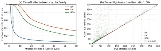
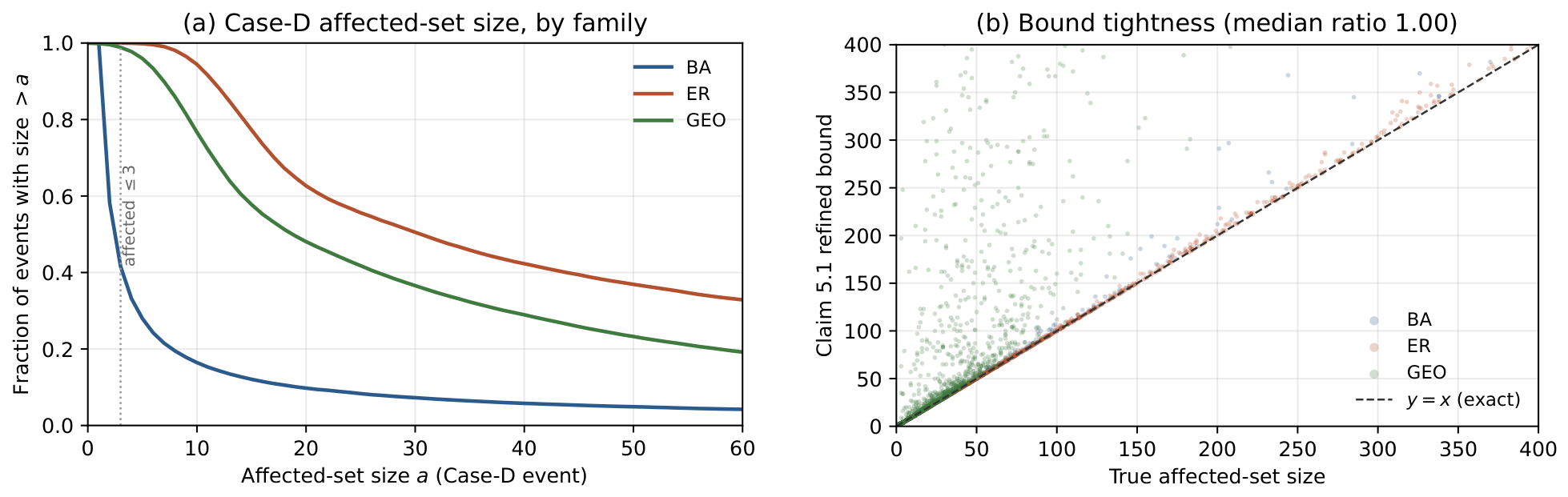
Across tree-edge records (BA/ER at –5000 and GEO at –2000 in the full three-family sweep, extended on BA to and ): the median affected-set size on BA is exactly 2 at every scale, with of Case-D events touching ≤3 NTEs—a scale-invariance strengthening the small-scale finding. ER’s median grows () and mean grows steeply (); GEO grows moderately. Claim 4’s refined bound correlates with the true affected-set size at (BA), (ER), (GEO), with median ratio —the bound is essentially tight in practice, and exactly tight for of events on BA, on ER, and on GEO. At the two largest scales the bound tightens further: exactly tight for of events at both and , with zero violations among the extension records. In Figure 3b, every event lies on or above the diagonal (the bound is never violated) and points above it are events where locally-known non-tree degrees include edges internal to the smaller side, which the bound must count but the true affected set excludes: a node’s slate knows its non-tree degree for free, but distinguishing cut-crossing from internal edges would require non-local information. This looseness is accordingly most common on GEO, where spatial locality keeps many non-tree edges within one side. Figure 3a’s curve shapes also preview the scheduling result: BA’s cliff-and-tail distribution (most events cheap, cost concentrated in a rare tail) is exactly the cheap/expensive separability that Section 7’s PRIORITY policy exploits, whereas ER’s uniformly high curve ( of events exceed size 10) leaves a scheduler the least to separate. Table 3 details the affected-set distribution.
Figure 3.
(a) Complementary CDF of Case-D affected-set size by family: BA is sharply concentrated (two-thirds of events touch NTEs), while ER and GEO have heavy tails (axis truncated at 60; tails extend further—a third of ER events exceed it). (b) Claim 4’s refined bound versus the true affected-set size; points cluster on (median ratio ), no point lies below it (the bound is never violated), and points above it are conservative cases where the locally-counted non-tree degree includes edges internal to the smaller side.
Table 3.
Affected-set size of Case-D events by family and scale. BA’s median is scale-invariant at 2; ER and GEO grow with n. “” is the fraction of events touching at most three NTEs. ‡ Scales added in revision: three graphs each (29,997 and 59,997 events), same generator and analysis.
7.3. Magnitude Predictor: How Much Model Is Needed?
The scheduler (Section 6) needs only to distinguish cheap from expensive Case-D events. We ask how much modelling this requires, comparing four points on a complexity spectrum—a zero-parameter threshold, a linear model, and two tree ensembles—all evaluated with by-graph train/test splits (never by row), so every number is a generalization to unseen graphs. Features are local slate quantities (endpoint degrees, non-tree degrees, , depth, edge-weight ranks, n, m); the label is “expensive” (refined bound ). Table 4 reports AUC and the Brier score (calibration; lower is better).
Table 4.
How much model is needed to predict Case-D cost. AUC (top) and Brier score (bottom), by-graph split, mean over 3 seeds. The threshold uses the slate’s and emits a raw bound, not a probability (no Brier). A linear model already recovers near-perfect discrimination where the threshold fails (ER, GEO); ensembles add negligible AUC but are extremely well calibrated.
Three findings, all reinforcing the same point. First, on BA, the zero-ML threshold on (exact slate state, computed for free) already reaches AUC , matching every model; no learning is needed there at all. Second, where the threshold fails (ER, AUC ), the gap is closed not by a nonlinear model but by a linear one: logistic regression jumps to , essentially matching the tree ensembles. The signal the threshold misses is not nonlinear—it is simply spread across the slate features in a way a linear combination recovers. Third, gradient-boosted trees are best on every family but beat logistic regression by at most a few thousandths of AUC, while being extremely well calibrated (Brier ): their predicted probabilities can be thresholded directly by the scheduler with confidence. The linear model also generalizes across families better than the ensembles (train BA, test GEO: for logistic regression versus GBDT, random forest). The overall conclusion is deflationary and, we think, the honest one: on the favorable topology the scheduling signal is already in the slate, and where it is not, it is nearly linearly recoverable from slate state—ensembles and, a fortiori, heavier models such as graph neural networks are not required for this task.
7.4. Scheduling Value Under Bounded Staleness
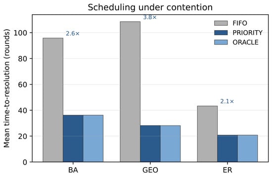
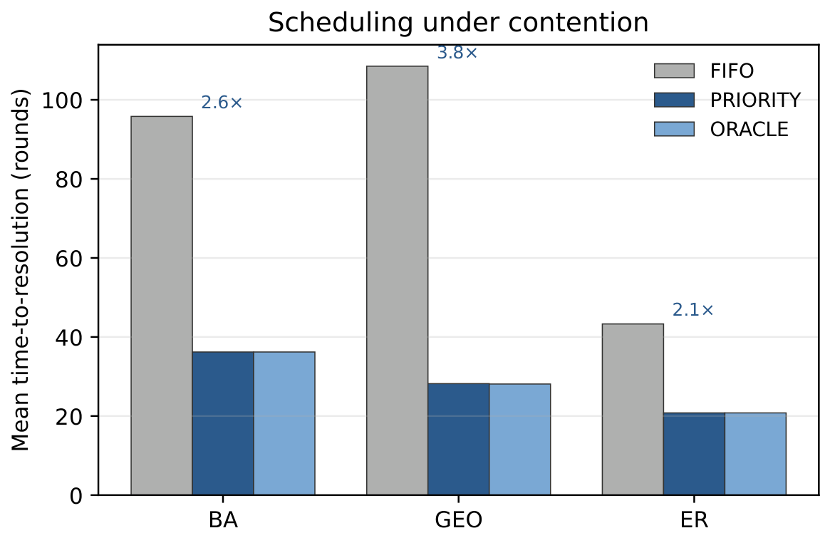
A stream of 4000 updates under a fixed per-round budget with headroom (a contended system), comparing FIFO, predictor-informed PRIORITY, and an ORACLE ceiling. PRIORITY improves mean time-to-resolution by (BA), (GEO), (ER) over FIFO, concentrated on cheap updates, and matches ORACLE in every family—the result is not predictor-limited. Correctness is unaffected throughout (Proposition 5). Table 5 reports time-to-resolution (TTR, rounds from arrival to completion), and Figure 4 shows the mean-TTR improvement of PRIORITY over FIFO across the three families.
Table 5.
Scheduling under contention. PRIORITY (predictor-informed) versus FIFO and an ORACLE ceiling; TTR in rounds. PRIORITY matches ORACLE throughout, so the result is not predictor-limited.
Figure 4.
Mean time-to-resolution under contention. Predictor-informed PRIORITY scheduling improves over FIFO by the annotated factors and coincides with the ORACLE ceiling in every family, showing the benefit is not limited by predictor accuracy.
7.5. Threats to Validity
Case-B-triggered swaps are modeled as cost-1 in the scheduling stream (rare, bounded by the same machinery); the scheduling experiment tests one contention level, one graph and seed per family (the benefit vanishes without queueing pressure); the static comparison charges NTE its worst case against measured GHS and uses the synchronous GHS variant. These are conservative simplifications that do not affect the qualitative conclusions. Finally, our evaluation is simulation-based, measuring protocol-level message and round costs rather than wall-clock performance on deployed hardware. A testbed deployment on real IoT or overlay infrastructure is the natural next validation step and is discussed in Section 9.
8. Implementation Considerations
The protocol is specified in the synchronous CONGEST model; this section maps that specification onto deployable systems and quantifies the per-node resources it needs.
8.1. From Modules to Executables
Each of the six modules of Section 4.4 is an event handler triggered by a message arrival or a local timer, so the natural implementation is a single-threaded, message-driven event loop per node—the execution model native to embedded operating systems for constrained devices and to actor frameworks on server-class overlays. The slate is a per-node record; no shared memory, global clock, or topology map is required. The synchronous-round abstraction is realized either by the coarse time-slotting common in duty-cycled sensor MACs or, on asynchronous networks, by running the protocol under a synchronizer [50]; the -synchronizer preserves round complexity at a constant-factor message overhead, which the worst-case charging of Section 7 already dominates. The model’s reliable-link assumption maps to any transport with per-link reliable in-order delivery: TCP between overlay peers, or link-layer acknowledgment and retransmission (e.g., IEEE 802.15.4 [51] ARQ) on wireless fabrics.
8.2. Per-Node Resource Footprint
State. A node v stores its slate—identifiers and costs for its incident edges, parent/child flags, the request sets, and the aggregation fields—totaling bits, plus the maximum-weight label of Section 4.2 at bits under polynomial weights. Concretely, with 16-bit identifiers and 32-bit weights, a degree-8 sensor node stores under 100 bytes of slate and a label of order 64 bytes: comfortably within Class-1 constrained devices (∼10 KB RAM) [52].
Messages. All three message types carry a constant number of fields (type tag, one edge identifier, one weight, one level), at most bytes of payload with the encodings above; every message fits in a single IEEE 802.15.4 frame (127-byte MTU) or one UDP datagram, so the -bit bound of Claim 1 is not merely asymptotic. Network-wide, the static algorithm’s worst case of messages amounts to KB of payload on a 1000-node Barabási–Albert fabric ().
Processing. Every handler performs integer comparisons per event; no floating point, cryptography, or dynamic allocation is required, and the degenerate-case handler is a constant-size guard.
8.3. Validation Path
The measured quantities of Section 7—messages and rounds—are the model-level proxies for transmission energy and latency respectively; converting them to joules and seconds for a concrete radio is a per-platform calibration. The natural validation sequence, planned as follow-up work (Section 9), is protocol emulation under a realistic radio and duty-cycle model (e.g., Contiki-NG/COOJA), followed by deployment on a public wireless testbed (e.g., FIT IoT-LAB) for wireless fabrics and containerized overlay deployment for the P2P and SDN settings.
9. Conclusions and Future Work
For the infrastructures that motivated this work (sensor fabrics, content and learning overlays, software-defined networks) the operative question is not whether a minimum spanning tree can be built, but whether it can be kept: maintained correctly and cheaply as the network changes underneath it. This paper answers the algorithmic core of that question with a complete treatment: a fully specified and proven construction protocol, an exact maintenance algorithm whose cost is characterized at scale, a precise boundary on what any distributed approach can achieve, and a scheduling layer that turns prediction into operational value. Along the way we established that the most ambitious use of prediction—shortcutting the maintenance computation itself—is impossible in a precise sense, a boundary that itself became a contribution and that shaped the design toward scheduling.
On construction, infrastructures gain a protocol they can implement from specification: the NTE algorithm is now fully specified and proved (Section 4)—the complete module-level design, the Cycle Theorem and Theorem NTE, and proofs of the complexity claims ( messages of bits in rounds) appear in the peer-reviewed literature for the first time. Experimentally, the algorithm’s proven worst case beats a measured synchronous GHS on rounds in every family tested (GHS taking – more) and on messages in the sparse regime ( fewer on Barabási–Albert graphs), with a density-dependent crossover on dense graphs—and the sparse regime is where the motivating applications live.
On maintenance—the operational core—the guarantees are proven and empirically characterized (Section 5 and Section 7): three of four update cases resolve in , and the fourth is resolved by ExactSwap within a bound shown essentially tight in practice (median ratio to the true cost). That cost is favorably distributed exactly where it matters: on scale-free graphs the median affected set has size 2 at every scale tested from to , a scale-invariance that considerably strengthens the case for the approach. The separation result (Proposition 4) delimits what any distributed algorithm can achieve here—exact replacement verification provably requires full-region search, a boundary with no centralized analogue—and directly shaped the final contribution: a scheduling-aware use of prediction that improves time-to-resolution – under contention while matching an oracle, and that needs less machine learning than one might expect, since the algorithm’s own state largely suffices and the residual signal is nearly linearly recoverable.
Several directions follow. The eager-caching question (Section 5.5) is the most consequential open problem: caching a replacement per tree edge works cleanly against one invalidation trigger (proven), but a second—a Case-B weight decrease silently undercutting an existing cache entry—remains unbounded; resolving it would reopen a genuine cost-reduction guarantee in the style of van den Brand et al. [19], and this paper has now located precisely where the difficulty lies. Edge insertions and deletions are treated in Section 5.4: the insertion decision is already an consequence of existing state (Proposition 3), deletion reduces to Case-D machinery, and a full treatment under realistic churn—mechanism, correctness, and evaluation together—is left to future work. A measured NTE simulator would replace the worst-case charging of Section 7 with measured message counts, sharpening the dense-graph crossover in NTE’s favor. Robustness sweeps for the scheduling result, across contention levels, graphs, and streams, are inexpensive with the pipeline in place; the benefit necessarily vanishes without queueing pressure, and mapping where it turns on is worth reporting. Finally, the three infrastructure settings that motivated this work each map directly onto the machinery developed here, with a distinct cost currency in each case. The readings below are protocol-level: they translate the measured message and round costs into each setting’s operational currency, and hold subject to the per-platform calibration described in Section 8. Energy-constrained sensor fabrics [1,2]: node death from battery depletion is precisely a Case-D-like event, and the scale-invariant median affected set of 2 means the energy cost of repairing the aggregation tree does not grow with deployment size on scale-free topologies—the currency is energy, and the O(1) resolution of Cases A–C means routine link-quality drift costs essentially nothing. Decentralized federated-learning overlays [4]: participant churn between training rounds is a stream of well-separated structural events, exactly the update model of Section 3—and the aggregation topology whose placement recent work optimizes [44] is precisely the structure our algorithm keeps minimal between placements— and the scheduling layer of Section 6 lets overlay repair be deferred to inter-round windows—the currency is training-round latency, and the oracle-matching PRIORITY policy shows that the deferral decision needs no heavyweight learning infrastructure. Software-defined multicast fabrics [6]: link failure triggers tree repair whose cost the controller must budget, and the tight per-update bound (median ratio ) gives the controller an accurate, locally-computable cost estimate before committing to a repair—the currency is reconfiguration latency. A testbed evaluation in one of these settings, replacing our protocol-level simulation with deployed-infrastructure measurements, is the natural next step and would complete the arc from formal specification to operational tool.
Funding
This research was supported by the Deanship of Scientific Research, Vice Presidency for Graduate Studies and Scientific Research, King Faisal University, Al Ahsa, Saudi Arabia [Grant number KFU264054].
Data Availability Statement
The datasets and seeded simulation code reproducing all experiments in Section 7 are available from the author on request.
Acknowledgments
During the preparation of this work, the author used Claude Opus 4.1 (Anthropic) to assist with language editing, improving the clarity of the manuscript, and preparing the LATEX source. AI-assisted output was carefully reviewed, revised, and verified by the author. The author directed and reviewed AI-assisted output, verified technical content, and takes full responsibility for the content of the published article.
Conflicts of Interest
The author declares no conflict of interest.
Appendix A. Detailed Pseudocode
The five modules below complete the specification begun with Algorithm 1 (the update aggregator, in the main text). All listings have been validated against the simulated trace of Section 4.5.
| Algorithm A1 Request Generator (at the session initiator) |
|
| Algorithm A2 Request Aggregator / Propagator (at node y, on Request from x) |
| Algorithm A3 Reply Aggregator (at node x) |
|
| Algorithm A4 Update Generator (at the update initiator D; D has no children) |
|
| Algorithm A5 Degenerate-Case Handler |
|
Note (Remark 1): the field is written by none of these modules; that field is populated only by the post-construction labeling pass described after Remark 1.
References
- Akyildiz, I.F.; Su, W.; Sankarasubramaniam, Y.; Cayirci, E. Wireless Sensor Networks: A Survey. Comput. Netw. 2002, 38, 393–422. [Google Scholar] [CrossRef] [Scilit]
- Njoya, A.N.; Thron, C.; Awa, M.N.; Ari, A.A.A.; Gueroui, A.M. Lifetime Optimization of Dense Wireless Sensor Networks Using Continuous Ring-Sector Model. Future Gener. Comput. Syst. 2022, 129, 212–224. [Google Scholar] [CrossRef] [Scilit]
- Chu, Y.h.; Rao, S.G.; Seshan, S.; Zhang, H. A Case for End System Multicast. IEEE J. Sel. Areas Commun. 2002, 20, 1456–1471. [Google Scholar] [CrossRef]
- Kairouz, P.; McMahan, H.B. Advances and Open Problems in Federated Learning. Found. Trends Mach. Learn. 2021, 14, 1–210. [Google Scholar] [CrossRef] [Scilit]
- Prigent, C.; Costan, A.; Antoniu, G.; Cudennec, L. Enabling Federated Learning Across the Computing Continuum: Systems, Challenges and Future Directions. Future Gener. Comput. Syst. 2024, 160, 767–783. [Google Scholar] [CrossRef] [Scilit]
- Kreutz, D.; Ramos, F.M.V.; Veríssimo, P.E.; Rothenberg, C.E.; Azodolmolky, S.; Uhlig, S. Software-Defined Networking: A Comprehensive Survey. Proc. IEEE 2015, 103, 14–76. [Google Scholar] [CrossRef] [Scilit]
- Gallager, R.G.; Humblet, P.A.; Spira, P.M. A Distributed Algorithm for Minimum-Weight Spanning Trees. ACM Trans. Program. Lang. Syst. 1983, 5, 66–77. [Google Scholar] [CrossRef] [Scilit]
- Awerbuch, B. Optimal Distributed Algorithms for Minimum Weight Spanning Tree, Counting, Leader Election, and Related Problems. In Proceedings of the 19th Annual ACM Symposium on Theory of Computing (STOC); Association for Computing Machinery: New York, NY, USA, 1987; pp. 230–240. [Google Scholar]
- Garay, J.A.; Kutten, S.; Peleg, D. A Sublinear Time Distributed Algorithm for Minimum-Weight Spanning Trees. SIAM J. Comput. 1998, 27, 302–316. [Google Scholar] [CrossRef] [Scilit]
- Faloutsos, M.; Molle, M. A Linear-Time Optimal-Message Distributed Algorithm for Minimum Spanning Trees. Distrib. Comput. 2004, 17, 151–170. [Google Scholar] [CrossRef] [Scilit]
- Lotker, Z.; Patt-Shamir, B.; Pavlov, E.; Peleg, D. Minimum-Weight Spanning Tree Construction in O(log log n) Communication Rounds. SIAM J. Comput. 2005, 35, 120–131. [Google Scholar] [CrossRef] [Scilit]
- Pandurangan, G.; Robinson, P.; Scquizzato, M. A Time- and Message-Optimal Distributed Algorithm for Minimum Spanning Trees. ACM Trans. Algorithms 2019, 16, 1–27. [Google Scholar] [CrossRef] [Scilit]
- Ragab, K.; Haque, A.U. A Minimum Spanning Tree Algorithm for Efficient P2P Video Streaming System. In Proceedings of the International Conference on Advanced Communication Technology (ICACT), Gangwon, Republic of Korea, 7–10 February 2010. [Google Scholar]
- Khan, J.I.; Haque, A.U. Maximizing Lifetime of Power-Limited Network with Active Minimum Spanning Tree Aggregation. In Proceedings of the 17th International Conference on Parallel and Distributed Computing and Systems (PDCS); ACTA Press: Cambridge, MA, USA, 2004. [Google Scholar]
- Díaz, S.; Méndez, D.; Schölzel, M. Dynamic Minimum Spanning Tree Construction and Maintenance for Wireless Sensor Networks. Rev. Fac. Ing. Univ. Antioq. 2019, 93, 57–69. [Google Scholar] [CrossRef] [Scilit]
- Xu, L.; Wen, D.; Qin, L.; Li, R.; Zhang, Y.; Lu, Y.; Lin, X. Minimum Spanning Tree Maintenance in Dynamic Graphs. Proc. Acm Manag. Data (PACMMOD) 2025, 3, 1–24. [Google Scholar] [CrossRef] [Scilit]
- Lykouris, T.; Vassilvitskii, S. Competitive Caching with Machine Learned Advice. J. ACM 2021, 68, 1–25. [Google Scholar] [CrossRef] [Scilit]
- Mitzenmacher, M.; Vassilvitskii, S. Algorithms with Predictions. Commun. ACM 2022, 65, 33–35. [Google Scholar] [CrossRef] [Scilit]
- van den Brand, J.; Forster, S.; Nazari, Y.; Polak, A. On Dynamic Graph Algorithms with Predictions. In Proceedings of the ACM-SIAM Symposium on Discrete Algorithms (SODA); Society for Industrial and Applied Mathematics: Philadelphia, PA, USA, 2024. [Google Scholar]
- Haque, A.U. Bounded Wait Communication for Systems with Distributed and Autonomous Components. Ph.D. Thesis, Kent State University, Kent, OH, USA, 2006. [Google Scholar]
- Chin, F.; Ting, H.F. An Almost Linear Time and O(V log V + E) Messages Distributed Algorithm for Minimum-Weight Spanning Trees. In Proceedings of the 26th IEEE Symposium on Foundations of Computer Science (FOCS), Portland, OR, USA, 21–23 October 1985; pp. 257–266. [Google Scholar]
- Peleg, D. Distributed Computing: A Locality-Sensitive Approach; SIAM: Philadelphia, PA, USA, 2000. [Google Scholar]
- Kutten, S.; Peleg, D. Fast Distributed Construction of Small k-Dominating Sets and Applications. J. Algorithms 1998, 28, 40–66. [Google Scholar] [CrossRef] [Scilit]
- Peleg, D.; Rubinovich, V. A Near-Tight Lower Bound on the Time Complexity of Distributed Minimum-Weight Spanning Tree Construction. SIAM J. Comput. 2000, 30, 1427–1442. [Google Scholar] [CrossRef] [Scilit]
- Elkin, M. A Simple Deterministic Distributed MST Algorithm, with Near-Optimal Time and Message Complexities. In Proceedings of the ACM Symposium on Principles of Distributed Computing (PODC), Washington, DC, USA, 25–27 July 2017; pp. 157–163. [Google Scholar]
- Khan, M.; Pandurangan, G. A Fast Distributed Approximation Algorithm for Minimum Spanning Trees. Distrib. Comput. 2008, 20, 391–402. [Google Scholar] [CrossRef] [Scilit]
- Huang, S.T. A Fully Pipelined Minimum-Spanning-Tree Constructor. J. Parallel Distrib. Comput. 1990, 9, 55–62. [Google Scholar] [CrossRef] [Scilit]
- Sleator, D.D.; Tarjan, R.E. A Data Structure for Dynamic Trees. J. Comput. Syst. Sci. 1983, 26, 362–391. [Google Scholar] [CrossRef] [Scilit]
- Karger, D.R.; Klein, P.N.; Tarjan, R.E. A Randomized Linear-Time Algorithm to Find Minimum Spanning Trees. J. ACM 1995, 42, 321–328. [Google Scholar] [CrossRef] [Scilit]
- Frederickson, G.N. Data Structures for On-Line Updating of Minimum Spanning Trees, with Applications. SIAM J. Comput. 1985, 14, 781–798. [Google Scholar] [CrossRef] [Scilit]
- Eppstein, D.; Galil, Z.; Italiano, G.F.; Nissenzweig, A. Sparsification—A Technique for Speeding Up Dynamic Graph Algorithms. J. ACM 1997, 44, 669–696. [Google Scholar] [CrossRef] [Scilit]
- Holm, J.; de Lichtenberg, K.; Thorup, M. Poly-Logarithmic Deterministic Fully-Dynamic Algorithms for Connectivity, Minimum Spanning Tree, 2-Edge, and Biconnectivity. J. ACM 2001, 48, 723–760. [Google Scholar] [CrossRef] [Scilit]
- Eppstein, D.; Italiano, G.F.; Tamassia, R.; Tarjan, R.E.; Westbrook, J.; Yung, M. Maintenance of a Minimum Spanning Forest in a Dynamic Plane Graph. J. Algorithms 1992, 13, 33–54. [Google Scholar] [CrossRef] [Scilit]
- Luo, M.; Qin, H.; Wu, X.; Xiong, C.; Xia, D.; Ke, Y. Efficient Maintenance of Minimum Spanning Trees in Dynamic Weighted Undirected Graphs. Mathematics 2024, 12, 1021. [Google Scholar] [CrossRef] [Scilit]
- Awerbuch, B.; Cidon, I.; Kutten, S. Optimal Maintenance of a Spanning Tree. J. ACM 2008, 55, 1–45. [Google Scholar] [CrossRef] [Scilit]
- Gupta, S.K.S.; Srimani, P.K. Self-Stabilizing Multicast Protocols for Ad Hoc Networks. J. Parallel Distrib. Comput. 2003, 63, 87–96. [Google Scholar] [CrossRef] [Scilit][Green Version]
- Peleg, D. Distributed Matroid Basis Completion via Elimination Upcast and Distributed Correction of Minimum-Weight Spanning Trees. In Proceedings of the 25th International Colloquium on Automata, Languages and Programming (ICALP); Springer: Berlin/Heidelberg, Germany, 1998; pp. 164–175. [Google Scholar]
- Foerster, K.T.; Korhonen, J.H.; Paz, A.; Rybicki, J.; Schmid, S. Input-Dynamic Distributed Algorithms for Communication Networks. Proc. ACM Meas. Anal. Comput. Syst. 2021, 5, 1–33. [Google Scholar] [CrossRef] [Scilit]
- Purohit, M.; Svitkina, Z.; Kumar, R. Improving Online Algorithms via ML Predictions. In Proceedings of the Advances in Neural Information Processing Systems (NeurIPS), Montréal, QC, Canada, 3–8 December 2018; pp. 9684–9693. [Google Scholar]
- Abdel-Wahab, H.; Stoica, I.; Sultan, F.; Wilson, K. A Simple Algorithm for Computing Minimum Spanning Trees in the Internet. Inf. Sci. 1997, 101, 47–69. [Google Scholar] [CrossRef] [Scilit]
- Hossain, M.A.; Khan, J.I. ZePoP: A Distributed Leader Election Protocol using the Delay-based Closeness Centrality for Peer-to-Peer Applications. In Proceedings of the 12th IEEE International Conference on Cloud Networking (CloudNet), Hoboken, NJ, USA, 1–3 November 2023. [Google Scholar] [CrossRef] [Scilit]
- Mokhtarian, K.; Jacobsen, H.A. Minimum-Delay Overlay Multicast. In Proceedings of the IEEE INFOCOM, Turin, Italy, 14–19 April 2013; pp. 1771–1779. [Google Scholar] [CrossRef] [Scilit]
- Mohammed, N.A.; Othman, M. A Load-Balanced Algorithm for Internet Gateway Placement in Backbone Wireless Mesh Networks. Future Gener. Comput. Syst. 2024, 150, 144–159. [Google Scholar] [CrossRef] [Scilit]
- Xu, B.; Zhao, H.; Cao, H.; Garg, S.; Kaddoum, G.; Hassan, M.M. Edge Aggregation Placement for Semi-Decentralized Federated Learning in Industrial Internet of Things. Future Gener. Comput. Syst. 2024, 150, 160–170. [Google Scholar] [CrossRef] [Scilit]
- Zhang, Y.; Duffield, N.; Paxson, V.; Shenker, S. On the Constancy of Internet Path Properties. In Proceedings of the ACM SIGCOMM Internet Measurement Workshop (IMW), San Francisco, CA, USA, 1–2 November 2001; pp. 197–211. [Google Scholar]
- Paxson, V. End-to-End Routing Behavior in the Internet. IEEE/ACM Trans. Netw. 1997, 5, 601–615. [Google Scholar] [CrossRef] [Scilit]
- Korman, A.; Kutten, S. Distributed Verification of Minimum Spanning Trees. Distrib. Comput. 2007, 20, 253–266. [Google Scholar] [CrossRef] [Scilit]
- Cormen, T.H.; Leiserson, C.E.; Rivest, R.L.; Stein, C. Introduction to Algorithms, 4th ed.; MIT Press: Cambridge, MA, USA, 2022. [Google Scholar]
- Prim, R.C. Shortest Connection Networks and Some Generalizations. Bell Syst. Tech. J. 1957, 36, 1389–1401. [Google Scholar] [CrossRef] [Scilit]
- Awerbuch, B. Complexity of Network Synchronization. J. ACM 1985, 32, 804–823. [Google Scholar] [CrossRef] [Scilit]
- IEEE Std 802.15.4-2024; IEEE Standard for Low-Rate Wireless Networks. IEEE: New York, NY, USA, 2024.
- Bormann, C.; Ersue, M.; Keränen, A. Terminology for Constrained-Node Networks; RFC 7228; Internet Engineering Task Force: Wilmington, DE, USA, 2014. [Google Scholar]

Disclaimer/Publisher’s Note: The statements, opinions and data contained in all publications are solely those of the individual author(s) and contributor(s) and not of MDPI and/or the editor(s). MDPI and/or the editor(s) disclaim responsibility for any injury to people or property resulting from any ideas, methods, instructions or products referred to in the content. |
© 2026 by the author. Licensee MDPI, Basel, Switzerland. This article is an open access article distributed under the terms and conditions of the Creative Commons Attribution (CC BY) license.