


Abstract
Published gaining-sharing knowledge (GSK) variants adapt scalar parameters and donor/selection policy to a single operating point. Dimension-Tiered GSK (DT-GSK) selects its configuration by dimension: an adaptive scaffold serves every tier, a deterministic, budget-exact final refinement runs once at , with the GSK vector-update equations retained; an exploratory interaction-structure memory supplies the refinement’s basis. Against six GSK-family baselines re-executed on five CEC suites under one budget-fair paired protocol, DT-GSK attains the best descriptive family-rank aggregate on CEC2017 (2.48) and CEC2013 (2.80), though Holm-corrected tests separate it from eGSK on either suite only at ; it is second behind eGSK at CEC2017 and on CEC2011 (Holm-significant loss). On AGSK’s strongest suite, the CEC2020 competition in which it was the runner-up, DT-GSK places fourth; the family panel corroborates AGSK’s published strength in this low-dimensional boundary regime, where every dimension-gated DT-GSK subsystem is inactive (). On CEC2013LSGO the comparison is family-internal: tied-first descriptive rank; paired tests do not separate DT-GSK from AGSK. Suite roles: CEC2017 selection-exposed; CEC2011/CEC2013 corroborative; CEC2020 pre-registered confirmatory; CEC2013LSGO post hoc. Direct isolations find no standalone benefit from that memory; coordinate axes outperform its basis: controlled negative results. All findings are scoped to the GSK-family panel.
1. Introduction
Bound-constrained continuous minimization under a hard evaluation budget (no derivatives, a fixed cap on objective evaluations, and landscapes that mix unimodal, multimodal, hybrid, and composition structure) is the regime that the CEC benchmark protocols formalize [1,2]. Population metaheuristics are the standard instrument in this regime, and the literature that produces them has grown to the point where its own surveys ask for fewer new metaphors and for more rigorous, statistically tested analysis of the algorithm families that already exist [3,4]. This paper follows that prescription. It stays inside one family, the gaining-sharing knowledge (GSK) algorithm and its published descendants, and asks a single design question. Published GSK variants adapt control to a single operating point. Can control instead be resolved by dimension, through an adaptive scaffold that reconfigures per tier and is closed by a deterministic, budget-exact refinement? And does that yield a measurable, statistically defensible improvement within the family? A second, subordinate question follows from the same design: whether a run’s own accepted moves carry recoverable coordinate-interaction structure that can be exploited at no extra objective evaluations, in particular at and . We answer the first affirmatively at the dimensions where tiering was demonstrated, and report the second as a controlled negative result.
GSK is a human-inspired metaheuristic whose junior and senior knowledge-transfer phases define the base operator family studied in this paper; every control parameter of the original algorithm is fixed for the whole run [5]. Its descendants attack that rigidity at the level of scalar parameters and donor or selection policy. AGSK draws its settings from a pool updated by success history [6], and APGSK extends those parameter-adaptation pools [7]. FDB-AGSK replaces the senior-phase guide with fitness–distance-balance selection after diagnosing premature convergence in its predecessor [8]. eGSK adds dual adaptive knowledge factors and a late local polish that relies on a sequential-quadratic-programming solver [9]. ATMALS-GSK tunes its control parameters through a memory of recent enhancement rates, plus a randomized local search whose computational overhead its authors acknowledge [10]. Each documented weakness in this lineage maps onto a named subsystem of the algorithm proposed here. Brittle fixed control, the family’s founding complaint, is answered by an operator-level, bandit-style credit-based adaptive operator selector with acceptance-gated pruning. Stagnation under GSK’s greedy selection, the failure mode behind the family’s escape and local-search additions, meets a hard-capped budget-safe escape and a restart that can never lose the global best. Late refinement that depends on a gradient-based solver or on randomized local search gives way to a deterministic, one-shot final polish: the deterministic refinement of the title, realized as the deterministic final polish (C1). And the weakness that no descendant addresses, recombination that treats every coordinate independently of the run’s own improvement history, is targeted by the interaction-structure memory (ISM), which this paper evaluates as an exploratory mechanism rather than as a source of the reported standing.
The common boundary of the GSK-family variants cited in this paper is what they adapt: scalar control parameters, donor and selection policy, or the population’s composition. Within that cited family (surveyed in Section 2, of which six algorithms form this paper’s comparison panel), none learns, or exploits, the interaction structure of the moves the run has already accepted. Yet a run under greedy selection may leave recoverable traces of that structure as a byproduct: every accepted move is a candidate signal about which coordinate pairs co-move on improving steps, and the signal costs no objective evaluations beyond those the run has already spent. Whether such a signal, once recovered, improves the optimizer is a hypothesis this paper tests; under the design reported here, and for GSK at these dimensions, it finds no detectable improvement. This paper proposes Dimension-Tiered Gaining-Sharing Knowledge (DT-GSK), which layers an adaptive configuration-and-budget scaffold and a deterministic final polish on the gaining-sharing vector-update operator, leaving that core unchanged, and is assessed through a controlled family evaluation; an interaction-structure memory feeds the polish basis and block crossover as a supporting mechanism. Section 2 bounds this gap against structure-learning approaches outside the family. The empirical question the paper answers is deliberately bounded as well: within the seven-algorithm GSK-family panel, under a budget-fair, reference-locked protocol, where does DT-GSK stand, and how does that standing change across dimension tiers?
The contributions are:
- C1—a deterministic final polish. A one-shot, RNG-free deterministic compass search executed on the eigenbasis of the ISM signed interaction matrix in the final budget slice (coordinate axes when the graph carries no signal). Every probe is charged through the strict budget-accounting path; the substreams driving the rest of the run are byte-identical whether the polish fires or not (its own probes still consume budget and can change the final incumbent); and no convergence guarantee is claimed. The contribution is the deterministic endgame itself, not the basis it searches along: a direct three-arm isolation at fixed enablement (Supplementary Materials Section S9.1) shows the endgame beating no refinement at both active dimensions, while the learned eigenbasis is beaten by the plain coordinate axes at () and, under the stated tie rule, at as well (). C1 is therefore claimed basis-neutrally, and the eigenbasis is retained as a specified, reproducible negative result rather than as a source of the benefit.
- C2—a dimension-tiered adaptive scaffold. The adaptive configuration engine (ACE), an exponential-moving-average credit-based adaptive selector over a pool of complete operator settings, with acceptance-rate gated pruning (ARGP) of unproductive arms; a tier-floored nonlinear population-size reduction (NLPSR) schedule, a variant of the APGSK NLPSR schedule, explicitly not claimed as new; a hard-capped budget-safe escape (BSE) seeded from a distance-filtered diversity archive; and a deep-stall full restart (multi-start) that preserves the global best. ACE, NLPSR, BSE, the archive, and the restart modify cited antecedents; we did not find ARGP’s acceptance-rate-gated arm-freezing rule among the surveyed GSK variants. C2 is claimed for the dimensions where tiering was demonstrated, and ; the tier is disclosed as mis-specified (Section 3.3).
- C3—a controlled, reproducible family evaluation. A 13-substream, append-only, prefix-locked random-number layer makes runs byte-stable and keeps each subsystem’s draws on a named substream, so component-level re-evaluation is exact; paired optimizer-independent seeds, one configuration fixed and verified by checksum, and versioned, immutable evidence releases bind every reported number to its release, from which the released analysis pipeline re-derives it in the declared supported environment. DT-GSK is evaluated against the original GSK and its five published descendants (AGSK, APGSK, FDB-AGSK, eGSK, and ATMALS-GSK, which together form the seven-algorithm GSK-family panel, every member of which was re-executed in this repository under that single protocol and seed schedule rather than quoted from its source publication) on five suites: the CEC2017 primary suite, the CEC2011 real-world optimization benchmark suite, the CEC2013 second comparison suite, the CEC2020 bound-constrained suite (pre-registered confirmatory), and the CEC2013LSGO large-scale suite (family-internal, post hoc). Every comparative finding in this paper is scoped to that panel. The within-family scope is a design choice rather than an omission—one code base, one budget protocol, and one evaluation harness confine implementation and environment confounds to the exceptions disclosed in Section 4 and Section 5 (the eGSK solver port and the documented self-initialization). Reported deltas are therefore read as algorithmic in origin, subject to those disclosed exceptions.
The interaction-structure memory is an online, decaying, evidence-gated coordinate-pair graph learned from strictly improving accepted moves without additional objective evaluations. It provides candidate linkage blocks for blockwise crossover and a candidate eigenbasis for the deterministic final polish (C1). However, the component isolation does not establish a consistent standalone performance contribution from ISM at the dimensions where it is active, and the function-class analysis reveals no systematic advantage on the hybrid or composition categories (Supplementary Materials, Sections S6.5 and S6.6). A direct basis isolation goes further: in the memory’s terminal exploitation channel, the polish basis, the learned eigenframe is outperformed by the plain coordinate axes at (Supplementary Materials, Section S9.1), so at that dimension the exploitation of the learned structure subtracts from a refinement that works without it. ISM is therefore positioned as a specified negative result rather than as a source of DT-GSK’s performance standing. Its inclusion provides a fully specified and reproducible investigation of structure learning from strictly improving accepted moves, while the paper’s principal contributions remain the dimension-tiered adaptive scaffold (C2), the deterministic final polish (C1), and the controlled, budget-fair family evaluation (C3).
The remainder of the paper is organized as follows. Section 2 reviews the GSK family, positions the interaction-structure memory against structure learning outside the family, and states the resulting gaps. Section 3 specifies DT-GSK: notation and the inherited base operators, the adaptive scaffold, the interaction-structure memory and its exploitation channels, the deterministic final polish, the frozen configuration, and the complexity and evaluation accounting. Section 4 reports the experimental study on the five suites, including the statistical analysis, the convergence subset, and measured runtime. Section 5 concludes with limitations and future work.
2. Related Work
Adaptation within the GSK family has been almost entirely scalar: each published variant adapts how strongly to move (rates, probabilities, population size), while the question of which coordinates to move together is left to a fixed, dimension-blind rule. The structure-learning literature outside the family answers that question, but pays for it with dedicated objective evaluations or a full sampling covariance. That gap (scalar control inside the family, evaluation-hungry structure learning outside it) is what the following comparison establishes, variant by variant (Table 1) and against the closest structure-learning lines on four dimensions (Table 2).
Table 1.
GSK-family review summary for the six published algorithms of the comparison panel: core mechanism, suites tested in the cited source, and key limitation. All entries are facts drawn from the cited publications; the table contains no results from this paper’s experiments.
Table 2.
Structure-learning taxonomy positioning ISM against differential-grouping and covariance/eigenbasis methods on four dimensions: update trigger, evaluation cost, what is learned, and how it is exploited. ISM updates from strictly improving accepted moves at no extra objective evaluations (not “free”: a per-generation decay plus an worst-case accumulation, with linkage blocks re-extracted every fifth generation at and every twentieth at ). Authored from literature facts drawn from the cited sources only.
2.1. The GSK Family: From Fixed Parameters to Adaptive Configuration
The gaining-sharing knowledge algorithm (GSK) is a human-inspired metaheuristic whose junior and senior knowledge-transfer phases define the base operator family studied in this paper [5]. Each individual learns from its fitness-ranked neighbors in the junior phase and from the elite, middle, and bottom strata in the senior phase; a knowledge-rate exponent shifts the per-dimension balance between the two over the run. Its original evaluation ranked it first on the CEC2017 score metric against ten classical and recent metaheuristics, and third by Friedman rank on the 22 CEC2011 real-world problems [5]. Every control parameter is fixed for the whole run (, , ): the limitation that later family papers identify as its central weakness.
The descendants attack that weakness at three levels: parameter adaptation, donor policy, and composite designs that add memory or a local search. AGSK introduced the family’s first adaptive parameter control: each individual draws its pair from a four-setting pool whose probabilities are updated from realized fitness improvements, combined with a dual-regime knowledge rate and linear population-size reduction in the L-SHADE lineage [6,11]. The adaptation, however, selects among four predefined scalar settings, and the evidence is confined to the ten CEC2020 functions at under budgets far larger, relative to dimension, than the CEC2017 protocol [6]. APGSK extended the same machinery with a second, negative-knowledge-factor pool activated after half the budget to re-diversify the population, a nonlinear population-size reduction schedule, an adaptive knowledge rate, and a much larger initial population [7]. Its evidence base remains CEC2020 at , where its comparisons against the CEC2020 winners show no statistically significant pairwise differences; what is adapted is still scalar parameter values, not where in the coordinate space the operators act [7].
FDB-AGSK redesigned AGSK’s donor policy instead of its parameters: the senior-phase guide is replaced by fitness–distance-balance selection, motivated by an explicit diagnosis of AGSK’s premature convergence on multimodal, hybrid, and composition functions [8]. The change concerns which individuals’ knowledge flows from, not which coordinates move together; and its benchmark evaluation used a budget (one tenth of the standard protocol) at , against AGSK variants only, with untested [8].
The two composite variants add memory and local refinement. ATMALS-GSK auto-tunes five control parameters (K, , , P, and a local-search probability) through Gaussian-weighted enhancement rates accumulated in an exponentially weighted moving-average (EWMA) memory and sampled by powered roulette-wheel selection, plus a shrinking-range local search on a small population fraction [10]. Within the GSK family as measured in that study, it ranks first on CEC2017 with eGSK second, its advantage growing with dimension while remains only competitive; its authors acknowledge the computational overhead of the memory machinery and local search [10]. Yet what that memory stores is which parameter values recently produced improvement, a hyperparameter memory; it carries no information about which coordinate pairs co-improve. eGSK layers three mechanisms on the base operator: a population-sum selection criterion, phase-specific self-adaptive knowledge factors activated after 75% of the budget, and a sequential-quadratic-programming (SQP) escape triggered in the same late window [9]. In its own CEC2017 study, it leads the compared family variants at but is competitive-only at , where it is significantly worse than AGSK [9]. Its late refinement depends on a gradient-based solver, and its adaptation remains scalar: no record of the run’s accepted-move structure informs the crossover or the escape.
The wider variant literature groups its own improvements into population, hybrid, strategy, and composite categories [12]. Population-side devices include Sobol-sequence initialization with Cauchy junior mutation and senior reverse learning [13], opposition-based learning with Cauchy mutation [14], and multi-population parallelism with Taguchi-orthogonal communication [15]. Strategy refinements range from historical-probability expansion of AGSK’s adaptation [12] to a reinforcement-learned controller for /. That controller’s authors report win/tie/loss tallies against basic GSK of 14/5/10 at and 16/4/9 at ; the instability they report is localized to a single function outside the training set rather than to the panel, whose tally is in fact stronger than the one [16]. Hybrid and operator-export lines transplant the junior/senior operators into DE [17], and the junior-phase operator into a whale-optimization host [18]; composite designs extend the family to multiobjective search [19] and to dual-population, multi-operator control with SHADE-style success histories [20,21]. Across all of these lines the adapted quantity is a scalar control parameter, a donor or selection policy, the population’s composition, or a grafted foreign operator. Within the cited GSK family, none of these variants learns, or exploits, the interaction structure of the moves the run has already accepted; Table 1 summarizes the six of these lines that form this paper’s comparison panel.
2.2. Structure Learning Outside the GSK Family
Learning structure from the search itself is well established outside the GSK family. The approaches separate on four axes (update trigger, evaluation cost, what is learned, and how it is exploited) on which Table 2 places each method and the interaction-structure memory. Three contrasts matter here. Differential grouping learns a hard variable partition in a dedicated offline stage, spending objective evaluations on pairwise probes and exploiting the result by decomposition into cooperative-coevolution subcomponents; its evidence lies at , with stated failure modes on overlapping interactions and region-dependent separability [22]. CMA-ES instead learns during the run at no additional objective evaluations, accumulating a full sampling covariance that reshapes every mutation, though a significant shape change takes on the order of evaluations of adaptation time [23]. Eigenvector-based crossover recomputes the eigenbasis of the current population covariance each generation (an instantaneous statistic, not a cumulative memory) at per generation [24]. Two further lines are adjacent rather than comparable. Adaptive operator selection adapts the choice of operator rather than the search geometry, and grounds the framing of DT-GSK’s ACE controller only [25,26]: ACE is not claimed to instantiate any specific bandit policy, and no regret guarantee transfers to the drifting rewards of an evolutionary run. Direct-search methods, in turn, refine a single solution without derivatives and carry no learned structure [27,28].
The interaction-structure memory occupies a point none of these covers. It updates online from accepted moves only, into a decaying (), confidence- and evidence-gated pair graph. It spends no additional objective evaluations (it learns from evaluations the run already made) at a compute-only cost of a per-generation decay plus an worst-case accumulation at –99 (thinned to every tenth generation at ) and one terminal eigendecomposition. What it learns is soft, signed pairwise evidence rather than a hard partition, a full sampling covariance, or an instantaneous eigenbasis; the distinction is not the type of object but the accepted-move-only, signed, decaying accumulation and a discrete exploitation that leaves the GSK operator numerics unchanged. Two boundaries are explicit. The component-isolation evidence for this memory stops at : it is isolated only on the bound-constrained suites, so the family’s standing is not attributed to it, in either direction, and the large-scale suite is a whole-algorithm family comparison, not a component contrast. And ISM is not claimed to recover the objective’s true interaction structure or to confer rotational invariance; it accumulates heuristic evidence from strictly improving accepted moves.
2.3. Positioning of DT-GSK Against the GSK Family
Three technical deficiencies, each traceable to the variants reviewed above, define the gap DT-GSK addresses. This subsection argues need only; effect is assessed in Section 4.
First, structure blindness. Every variant in Table 1 adapts scalar control parameters, donor or selection policy, or population composition. Within the GSK-family variants cited in this paper (a bounded review of the GSK lineage rather than an exhaustive systematic search of the wider metaheuristic literature), none learns or exploits the interaction structure of the moves the run has already accepted. The survey scope is explicit and reproducible. It covers the original GSK and the published GSK-family variants of Table 1. For each, we inspected the stated adaptation target (control parameters, donor/selection policy, or population sizing) for any online, evaluation-free learning of coordinate-pair interaction structure. The resulting claim is bounded to this lineage; it is not a state-of-the-art priority claim over the wider literature. DT-GSK’s interaction-structure memory and its two active consumers, the linkage-aware block crossover and the signed-graph eigenframe polish (an ISM-block subspace local search is implemented but not enabled in the frozen configuration), are designed for exactly this quantity.
Second, endgame refinement without determinism or budget safety. The family’s two late-refinement mechanisms are eGSK’s SQP escape, which depends on a gradient-based solver [9], and ATMALS-GSK’s randomized shrinking local search, whose computational overhead its authors acknowledge [10]. DT-GSK’s deterministic final polish is instead one-shot, RNG-free, hard-capped by the final budget slice, and runs on the eigenbasis the ISM has already learned; no convergence guarantee is claimed for it.
Third, regime-limited adaptation evidence. AGSK’s and APGSK’s adaptive machinery was evaluated on CEC2020 at [6,7], and FDB-AGSK at a budget without [8]. The two strongest variants also share a low-dimension weakness on CEC2017: eGSK is significantly worse than AGSK at [9], and ATMALS-GSK is competitive-only there [10]. Across these variants the axis of adaptation is the parameter value: ATMALS-GSK, for instance, drives five scalar parameters from a Gaussian and weighted-moving-average memory of their past effect on fitness, but resolves them within one control regime that is not itself a function of problem dimension [10]. This paper meets that regime head-on: CEC2020 at serves as the pre-registered confirmatory suite (Section 4.5). DT-GSK responds on an orthogonal axis, resolving the control regime by dimension rather than only the values inside it: a dimension-tiered adaptive scaffold, resolved from a single frozen configuration per dimension tier. Its parts are the ACE credit-based selector with ARGP pruning, the tier-floored NLPSR schedule (a variant of the APGSK NLPSR schedule, not claimed as new [7]), the budget-safe escape in the JADE/SHADE archive lineage [21,29], and a deep-stall restart that preserves the global best.
The bounded gap is therefore: within the GSK operator style, exploit the interaction structure of the moves the run has already accepted, at the upper tested tiers ( and ), without spending any additional objective evaluations and without replacing the base operator. The junior and senior gaining-sharing vector-update equations are inherited unchanged [5], while the surrounding generation mechanics are modified; DT-GSK’s contribution is an adaptive configuration-and-budget scaffold, a deterministic final polish, and a controlled family evaluation layered on those inherited equations, with an interaction-structure memory as a supporting mechanism. Whether this closes the gap is an empirical question, answered within the seven-algorithm GSK-family panel in Section 4.
3. Proposed DT-GSK Algorithm
DT-GSK retains the junior and senior gaining-sharing vector-update equations of GSK verbatim (Equations (1)–(4)). What it modifies is the generation mechanics that surround them: the crossover mask (linkage blocks, Equation (5)), tie handling in the greedy selection (≤, Equation (9)), the floor, an optional DE trial arm, the senior partition, and the population size (NLPSR). On top of that core, it layers four kinds of machinery: control, budget, structure-memory, and polish. The contribution boundaries are marked explicitly throughout: no new base operator is claimed, the dimension-tiered adaptive scaffold is C2, the deterministic final polish is C1, and the determinism layer is C3; the interaction-structure memory is a supporting mechanism, not a contribution. Every mechanism below is presented as proposed and fully specified, and each design constant is either justified in one sentence or labeled a frozen default of the single shipped configuration.
3.1. Notation and Base-GSK Recap
Table 3 collects the core problem, population, and base-GSK symbols; the subsystem symbols are introduced with their sections, and the RNG substream key with the reproducibility material (Supplementary Materials, Section S5). Throughout, symbols keep one casing and one meaning across prose, equations, pseudocode, and tables.
Table 3.
Core notation: problem, population, and base-GSK symbols used in the pseudocode (Algorithm 1) and the equation registry (Equations (1)–(13)). Subsystem symbols are defined with their sections (Tables 6 and 8); per-equation GSK trial/mask symbols (, , ) are defined in place, and constants take the frozen-configuration values (Table 10).
We consider bound-constrained minimization of over the box , whose bounds are given per coordinate (the uniform case , recovers the scalar box ), under a fixed evaluation budget MaxFES. GSK [5] evolves a population P through a junior (gaining) and a senior (sharing) knowledge-transfer phase. In the junior phase, each individual at fitness rank draws its knowledge sources from its rank neighbors and one random peer, Equation (1). In the senior phase the sources come from the top, middle, and worst partitions of the ranked population, with the outer group sizes set by the partition fraction p, Equation (2). The expected number of coordinates treated by the junior rule decays with the consumed budget fraction through the schedule of Equation (3), where is the schedule exponent (frozen default ). Both phases apply the gaining-sharing update of Equation (4), where scales the step and is the sign of the fitness comparison between the individual and the knowledge source its phase compares against. That source is the random peer in the junior phase and the middle-group source in the senior phase, exactly as in the published operator. Out-of-bounds components are repaired to the midpoint of the parent and the violated bound, Equation (8), the rule introduced with JADE [29] and carried through the L-SHADE lineage [11], and survivors are chosen by greedy elitist selection, Equation (9): a child replaces its parent if it is no worse (≤; ties accepted).
These four elements (the junior/senior operator with its index rules, the junior-dimension schedule, the midpoint bound repair, and the greedy selection) are inherited from their cited sources [5,11] with their vector-update numerics unchanged; the only relaxation is the ≤ tie-handling in selection (accepting equal-fitness trials). For single-source reference, the complete frozen set of update rules for DT-GSK is reproduced below: Equations (1)–(4), (8) and (9) are the inherited rules just discussed. Equation (5) (crossover mask) is discussed with the linkage channel in Section 3.4. Equations (6), (7) and (10) belong to the scaffold of Section 3.3. Equations (11) and (12) define the structure memory and the polish (Section 3.4 and Section 3.5). Finally, Equation (13) defines the determinism layer (Section 3.7).
At the rank boundaries the neighbour pair is taken from the two nearest interior ranks: for the best individual () and for the worst (), as in the reference GSK implementation [5].
The fraction p is population-wide below . At the frozen profile enables a conditional two-rate partition: while the trailing ten-generation mean acceptance is at most , the worse-ranked half of the population draws its senior sources with and the better-ranked half keeps ; whenever acceptance is above that floor, the single rate is used for the whole population.
Each coordinate joins the junior phase with marginal probability , so is the expected, not the realized, junior-coordinate count. The assignment is an independent per-coordinate Bernoulli draw only on the rows that take the scalar mask; on a linkage-blockwise row (Equation (5)) a single draw is shared across a whole block, so coordinates within a block are perfectly correlated and the realized count is more dispersed than the independent case.
Here are the signs of two different fitness comparisons: the junior phase compares the random source to , whereas the senior phase compares the middle source to . Both follow the same convention: when the compared source is fitter than , so that the step is oriented towards it, and otherwise (an exact tie takes ).
Here is not a single frozen configuration value but the rate carried by the ACE arm that individual i drew this generation, so it varies per individual and per generation over the arm pool. It is additionally floored at with by tier, which raises the low- arms above their nominal rates at every . Finally, a force-nonzero guarantee applies after mask assembly in both modes: if a row’s mask would leave the trial identical to its parent, one coordinate is set at random so that every trial differs from its parent in at least one coordinate.
The tie-accepting form above is the base rule and is what runs at . At the late-acceptance clip can replace it, late in the budget and after a stall streak, with the strict test at (a distinct symbol from the stagnation tolerance ), which rejects ties; the clip’s own gates are given in Supplementary Section S5.
where 2,147,483,646 is the child-seed modulus (Supplementary Material, Section S5).
3.2. Architecture Overview and Execution Order
DT-GSK ships as a single frozen configuration, which resolves every setting from the problem dimension and is hash-frozen (Section 3.7); no per-suite or per-run tuning exists on the four bound-constrained suites, and the single large-scale exception, two linkage-block-size entries for CEC2013LSGO’s native dimensions, is disclosed in Section 3.7 and Supplementary Section S7. Table 4 shows how the subsystems compose around the unchanged GSK vector-update equations, Algorithm 1 gives the canonical loop, and Figure 1 and Figure 2 chart the control flow of base GSK and DT-GSK, respectively.
| Algorithm 1 Pseudo-code of the DT-GSK algorithm. The junior and senior gaining-sharing vector-update equations are retained unchanged; the generation around them is not: crossover masking, tie handling, the population size, and the senior partition are all modified. The added subsystems and their fixed execution order are listed in Section 3. | |
| Require: objective f, dimension D, bounds , budget , seed ▷ budgets: Section 3.8 | |
| Ensure: global best solution | |
| Initialization | |
| 1: | Initialize the interaction graphs ▷ allocated only at |
| 2: | Set and the GSK parameters |
| 3: | Open the 13 RNG substreams for dimension D |
| 4: | Create a random population in |
| 5: | Evaluate for all i and set the global best |
| 6: | while do |
| Adapt and build trials | |
| 7: | Reduce by the NLPSR schedule ▷ Equation (6) |
| 8: | Assign each individual an ACE arm ▷; a sixth DE arm at |
| 9: | Count the gained and shared dimensions ▷ Equation (3) |
| 10: | Apply the junior gaining-sharing phase |
| 11: | Apply the senior gaining-sharing phase |
| 12: | Form the crossover mask: linkage block on some rows, mask on the rest ▷ Equation (5) |
| 13: | if DE arm: overwrite the masked coordinates with a DE/rand/1 mutant ▷, |
| 14: | Repair the out-of-bounds coordinates |
| 15: | Evaluate the maximal prefix of that fits the budget ▷ the rest are non-selectable |
| 16: | Greedily keep each no-worse trial and update the diversity archive ▷ Equation (9) |
| Learn, escape, and refine (dimension-gated) | |
| 17: | if : update the interaction-structure memory ▷ Equation (11) |
| 18: | Update the ACE credit and prune stalled arms (ARGP) |
| 19: | if stagnating: apply the budget-safe escape ▷ Equation (10) |
| 20: | if in the endgame slice: charged coordinate local search on the elites |
| 21: | if : polish the working incumbent once, in the final slice ▷ Equation (12) |
| Update and restart | |
| 22: | Update the global best |
| 23: | if deep-stalled: restart the population, keeping |
| 24: | end while |
| 25: | return |
| Note. The linkage block is learned at (random otherwise) and confidence-gated; the local search enters at of the budget below and at above, under its evaluation cap and cooldown; and the upper-tier controllers are cross-cutting (they act inside the reduction, trial-construction, acceptance and escape steps above and gate the local search) as detailed in Section 3. | |
Table 4.
Architecture of DT-GSK: the eight subsystems composed around the unchanged GSK vector-update operator, with each subsystem’s category (inherited/scaffold/dimension-gated), active tier, and role. Every objective evaluation (trials, escapes, local-search and polish probes, restart resamples) is charged through one budget controller, and all randomness draws from the 13-substream RNG rail (Equation (13)); the deep-stall restart preserves the global best.
Figure 1.
Flowchart of the base GSK algorithm of Mohamed et al. [5], redrawn here from that paper’s description: a single generation loop of fitness evaluation, gained–shared dimension counting, the junior and senior gaining-sharing knowledge phases, and greedy update, repeated until the termination criterion is met. The figure depicts prior work and contributes nothing new; it is included so the DT-GSK flowchart in Figure 2 can be read against its parent.
Figure 2.
Flowchart of the DT-GSK algorithm, drawn in the same style as Figure 1 for direct comparison. The GSK core (fitness evaluation, dimension counting, the junior and senior phases, and the update) is retained; the boxes with a light shaded fill are the mechanisms DT-GSK adds: the nonlinear population-size reduction (NLPSR) and the ACE selector with acceptance-gated pruning, the linkage-aware block crossover, the dimension-gated interaction-structure memory, the coordinate local search, the budget-safe escape with deep-stall restart, and the one-shot deterministic final polish. At the upper-tier controllers are cross-cutting rather than a single stage: they act within the population-reduction, trial-construction, acceptance, and escape steps above (and gate the local search), so they are not drawn as a separate node. The global best is preserved throughout.
One configuration asymmetry follows from running each algorithm at its own reference configuration rather than at a common population size. The six comparators use at every dimension (the setting of the family’s shipped reference implementations re-executed here, which for some comparators differs from the dimension-scaled populations of their source papers), whereas DT-GSK initializes before the NLPSR reduction; at , that is 500 against 100. All seven receive the identical evaluation budget, so the difference lies in how each algorithm spends that budget rather than in how much it is given. Both settings are protocol-conformant: each suite’s protocol fixes its evaluation budget and run count and prescribes no population size. We state it explicitly because population size is a design choice that can materially affect upper-tier behavior, and a reader comparing at should know the initial populations differ by a factor of five. A common-initial- replication was carried out on CEC2017, with DT-GSK’s own reduction law and tier floors retained: at the comparators’ , DT-GSK remains first at and second at , 50 and 100, with the paired difference significant only at and (Supplementary Materials, Section S9.2). On CEC2013LSGO the corresponding ratio at initialization is fifty-fold; it is disclosed but not controlled (Supplementary Materials, Section S7).
Within one generation the subsystems execute in the fixed order below, which Algorithm 1 lists and Figure 2 charts.
- (1)
- Nonlinear population-size reduction (NLPSR).
- (2)
- Operator-arm sampling by the adaptive configuration engine (ACE).
- (3)
- Junior/senior trial construction and crossover masking.
- (4)
- Bound repair and evaluation.
- (5)
- Elitist acceptance and the diversity-archive update.
- (6)
- At , the interaction-graph (ISM) update from strictly improving accepted moves.
- (7)
- The operator-credit update and acceptance-rate gated pruning (ARGP) of the operator pool.
- (8)
- Stagnation escape by the budget-safe escape (BSE) mechanism.
- (9)
- The charged coordinate local search.
- (10)
- At , the one-shot deterministic final polish in the final budget slice.
- (11)
- Global-best update.
- (12)
- The deep-stall restart check.
The upper-tier controllers do not form a separate step in this order: they are cross-cutting, acting within population reduction (the subspace-sampling floor), trial construction (frozen-streak broaden and late linkage random-mix), acceptance (the late-acceptance clip and the basin-memory update), and the budget-safe escape (basin-novelty reseed); a budget/ROI gate additionally gates the local search (a matching hook exists on the escape but never blocks it in the frozen configuration). A step written “if ” in Algorithm 1 is inactive below tier d. Every subsystem is elitist with respect to the working population (it cannot return a population whose best is worse than the incumbent it was given), with one deliberate exception: the deep-stall restart resamples the working population outright (Section 3.3.5). The global best is held separately from the working population, is never re-initialized, and is what the run returns; it therefore never loses ground. Dimension-tier gating is stated once and holds everywhere. The blockwise linkage mask is active from , applied to a tier-dependent fraction of the population, with the remainder keeping the per-coordinate mask of Equation (5). The interaction-structure memory and the deterministic final polish activate at , while the coordinate local search is active at all tiers. The protective controllers activate at . Below its tier, each gated block is a no-op. Table 5 gives the activation pattern.
Table 5.
Subsystem activation across the frozen configuration’s four dimension tiers (, 20–49, 50–99, ; the CEC benchmark dimensions are the respective tier representatives). on/off gives the activation state per tier and the last column gives the tier-varying parameters. The threshold structure follows the frozen parameter table (Table 10). Within the tier, the linkage mask carries its own gate (Table 4), so it is additionally inactive at the CEC2020 cells.
3.3. Dimension-Tiered Adaptive Scaffold (Contribution C2)
The scaffold answers a control and budget problem: a single frozen configuration must remain usable from to without per-problem tuning, under a greedy selection rule (a trial replaces its parent when no worse, ≤; Equation (9)) that can starve the search of accepted moves. Its five sub-mechanisms are labeled honestly: ACE, NLPSR, BSE, the diversity archive, and the deep-stall restart are modifications of cited antecedents; we did not find ARGP’s acceptance-rate-gated arm-freezing rule among the surveyed GSK variants. The individual contribution of the scaffold subsystems is examined in a remove-one component study in the Supplementary Materials (with the interaction-structure memory held off in every cell); ARGP, the final polish and the deep-stall restart are prespecified exclusions from that study and are therefore not isolated. A direct isolation of the memory overlay itself is reported in the Supplementary Materials (Section S6.5) and finds no significant standalone benefit at the memory’s active tiers. The dimension-tiering itself, resolving control by dimension rather than at a single fixed operating point, is likewise not isolated by the component studies above. A controlled tiered-versus-tier-constant contrast (Supplementary Materials, Section S9.3) separates the two at and against a high-dimension transplant, while at a low-dimension transplant outperforms the shipped configuration. C2 is therefore claimed for the dimensions where tiering was demonstrated, with the tier disclosed as mis-specified, rather than as evidence that dimension-tiering is individually causal at every tier. Here each mechanism is specified with its trigger, timing, and cost. Table 6 lists the symbols this subsection introduces.
Table 6.
Scaffold notation (Contribution C2): symbols for the ACE/ARGP operator controllers (Section 3.3.1 and Section 3.3.2), the tier-floored population schedule (Section 3.3.3), and the budget-safe escape, diversity archive, and restart machinery (Section 3.3.4 and Section 3.3.5). Constants take the frozen-configuration values (Table 10).
3.3.1. ACE: Bandit Control of the Operator Pool
A fixed triple that suits one landscape or one dimension tier is brittle on another. AGSK adapts from a fixed pool by success history [6], and APGSK widens the adapted parameter pools [7]; both adapt at the parameter level. ACE instead adapts at the operator level: it maintains a pool of five complete operator settings (a sixth, optional differential-evolution arm joins at the mid-dimension tiers, below)—arm 3 is the GSK-pure setting —and draws one arm per individual per generation. Each arm’s per-generation reward is its aggregate fitness improvement , the summed over the individuals that drew it, not a raw acceptance count. The credit target is mixed by an exponential moving average at learning rate (frozen default) into the selection-probability vector , which is projected onto the floored simplex , Equation (7). When the generation improves in aggregate () the target is the full-pool share . When it does not, the target is restricted to the arms that individually improved. When no arm improves, or the aggregate is exactly zero, is held unchanged apart from that projection. The floor keeps every arm alive for exploration, and the improvement-weighted update is in the spirit of SHADE’s success history [21]. At the credit assignment splits into a top/bottom improvement memory, and for an optional differential-evolution arm joins the pool [30]. The bandit literature grounds this framing of operator selection as a dynamic exploration–exploitation problem [25,26]; ACE is not an instance of those algorithms, and no regret bound is claimed for it. ACE is control-plane only: it consumes no objective evaluations, and its per-generation cost is for arms (five, or six with the optional mid-tier DE arm).
3.3.2. ARGP: Acceptance-Rate Gated Pruning
The probability floor that keeps ACE exploring also forces draws of arms that have stopped producing accepted moves. ARGP resolves this. After a warm-up of 0.15 of the budget, any arm whose acceptance rate over a rolling window of generations falls below the tier threshold (0.02, tightened to 0.010 at ) is soft-frozen to the probability floor rather than removed, provided at least two arms remain active. Subsequent draws therefore concentrate on productive operators. The freeze is recoverable: a frozen arm is re-activated as soon as its windowed acceptance climbs back to , so ARGP redistributes operator budget rather than permanently retiring it. Its bookkeeping cost is per generation.
3.3.3. NLPSR: Tier-Floored Population-Size Reduction
NLPSR is explicitly not claimed as new. It keeps the concave reduction shape of APGSK’s NLPSR schedule [7] and modifies its endpoints, starting from the dimension-scaled and bottoming at a tier-specific floor (25 at , 12 below) rather than a fixed minimum, Equation (6). Each generation the worst surplus rows are culled. The tier floor is the modification that preserves enough parallel samples for the structure memory at upper tier while letting low tiers shrink further. Table 7 hand-checks the two schedules at .
Table 7.
Worked numeric example at : the tier-resolved NLPSR schedule of Equation (6) (with , ; rounded half-up) and the junior-dimension schedule of Equation (3) (with ), against the consumed budget fraction x. Milestones mark the frozen configuration’s gates; all values are analytic evaluations of the schedule formulas.
3.3.4. BSE and the Diversity Archive: Budget-Safe Escape
Greedy selection over a shrinking population can stagnate: no accepted moves, collapsing diversity, and a flat improvement signal. BSE monitors these symptoms over a window of generations. At it uses a triple-trigger detector (signal window 10, scale-aware tolerance , acceptance floor 0.10, diversity floor 0.35); below it falls back to a single stagnation trigger, for which the acceptance and diversity floors are inactive. When triggered it first perturbs the worst fraction of the population with heavy-tailed Cauchy draws, Equation (10), sparing the frozen elite: the top rows by fitness, exempt from both the rescue and the restart (Supplementary Material, Section S5), which anchors the equation’s “unfrozen” qualifier; a successful rescue, one that lowers the incumbent best, cancels the restart for that generation, and only when the rescue fails does BSE then reseed part of the population from a diversity archive: a Cauchy-rescue-then-partial-restart design in the external-archive lineage of adaptive differential evolution [21,29,30]. The archive is a distance-filtered diversity store, not a fitness-ranked elite set. A candidate is admitted only when it is at least a normalized-L2 distance of from every stored point. Once the store is full ( at every dimension in the frozen configuration; the sizing is the fallback used only when no absolute cap is set, and is inert here), a new admission overwrites the spatially closest entry. There is no fitness-quality admission or eviction criterion. The modification that names the mechanism is its budget safety: BSE is hard-capped by a maximum restart count (4 at and , else 2) and by a stop fraction beyond which it is disabled, so as a design fact it can never overshoot MaxFES. When it fires, its cost is , and its restart evaluations are charged like any others (Section 3.8).
3.3.5. Deep-Stall Restart with the Global-Best Invariant
BSE perturbs within the current basin; a search that is deeply stuck needs more. The deep-stall full restart (multi-start) re-initializes the working population when the incumbent has been frozen for at least of the budget, subject to a cooldown (0.15 of budget) and a stop fraction (0.9). It draws up to fresh individuals, truncated when little budget is left, and the resampled points are evaluated through the same budget as any other trial. A separate global-best pair is preserved across restarts and is what the run returns. This yields the restart-never-loses-ground invariant, a design property of the implementation: no restart can worsen the reported result, because the global best is never re-initialized. A minimum-budget guard (20,000 evaluations) keeps tiny budgets inert, so the mechanism cannot perturb short runs.
3.4. Interaction-Structure Memory and Linkage-Aware Exploitation (Supporting Mechanism)
As established in Section 2, no cited GSK-family variant learns or exploits the interaction structure of the moves a run has already accepted. Outside the family, structure learning is available, but at a different cost or mechanism. Differential grouping spends a dedicated offline budget of pairwise-probing objective evaluations, quadratic in the dimension, before optimization starts [22]. Covariance matrix adaptation learns a full sampling covariance from selected steps [23]. Eigenvector-based crossover recomputes the population-covariance eigenbasis every generation [24]. The design observation behind the interaction-structure memory is that greedy selection already exposes this signal for free: each accepted move records which coordinate pairs moved together on an improving step, and reading that record consumes none of the run’s evaluation budget. Table 8 lists the symbols this subsection and the final polish use.
Table 8.
Interaction-structure memory and eigenframe-polish notation (supporting mechanism, Section 3.4; Contribution C1, Section 3.5). Constants take the frozen-configuration values (Table 10); the graph-confidence functional is detailed in Supplementary Materials, Section S5.
The interaction-structure memory accumulates this evidence in a decaying interaction graph, updated only from strictly-improving accepted-move deltas at learning rate . The retained graph is decayed by at each update so that stale evidence fades, Equation (11). There is the accepted move of individual i, contributed as an improvement-weighted, per-move -normalized outer product. Two of the four state components, the co-evolving interaction matrices, share this decay–accumulate form; both are symmetrized with a zero diagonal. A non-negative magnitude graph (built from ) supplies the confidence gate and the linkage blocks. A signed graph (built from the raw ) supplies the eigenframe-polish basis of Section 3.5. The full per-move weighting, normalization, and support bookkeeping are in the Supplementary Materials (Section S5). Because the graph is allocated only at , the operative confidence gate there is , superseded by an adaptive rolling-window median of recent confidences, floored at ; a block is used only when . The graph is updated every generation and its linkage blocks are re-extracted every 5 generations (at , every 10 and 20 generations respectively) after a warm-up of 0.10 of the budget. Formally, is a signed, decaying second-moment (co-movement) statistic over coordinate indices: it is covariance-like in construction, and the terminal polish of Section 3.5 operates on its eigenbasis, a covariance-eigenbasis operation. The novelty is therefore not that the learned object is of a fundamentally new type. It is that the object is accumulated only from strictly-improving accepted moves (ties and DE-arm moves are excluded, and local-search moves enter at weight ), then held signed and decaying, and exploited discretely through block masks and the polish eigenbasis, all while the GSK vector-update numerics are left unchanged. The interaction memory records which coordinate indices co-move on improving steps; it is not a recovered map of the objective’s true variable interactions. ISM consumes no extra objective evaluations, since it observes moves the run already evaluated. It is not free of cost, however. At each generation costs to decay the graph, plus to accumulate the k strictly-improving accepted-move outer products (). It also stores four decaying accumulators: the two interaction matrices (magnitude and signed ), the co-occurrence support C, and the per-dimension activity (Section 3.8).
The learned structure is exploited through two active channels (Table 9): the linkage-aware block crossover and, terminally, the eigenframe polish of Section 3.5. A third channel, an ISM-block subspace local search, is implemented but not enabled in the frozen configuration. The first active channel is the linkage-aware block crossover. For a tier-dependent fraction of the population, about at and at 20–49, the per-coordinate mask of Equation (5) is replaced by a linkage-block mask that copies a whole block together. The mask is refreshed every 20 generations () or 10 (). The blocks are not contiguous coordinate ranges: the random groups are permutation chunks (arbitrary index subsets) and the ISM-supplied groups are learned graph components. Below the blocks are random groups of size 5, a variant of the inherited mask, not a claimed contribution. From each blockwise row draws its blocks from the learned ISM graph with probability , and from the random permutation partition otherwise (block size 10), so the learned structure supplies about half of the blockwise rows rather than all of them. The graph itself is active only for and is re-extracted into blocks every 5 generations at and every 20 at . The graph’s top-k blocks could also define a bounded subspace (at most 20 coordinates) for a structure-aware local search, but this ISM-block subspace variant is not enabled in the frozen configuration, which runs a charged axis-aligned coordinate local search instead (the second active channel, the eigenframe polish, is Section 3.5). Either way the local-search probes are charged through the normal budget path.
Table 9.
How strictly improving accepted moves become exploitable structure: strictly improving acceptance events update the interaction-structure memory (ISM) graph EMA (Equation (11)), whose confidence-gated blocks feed the linkage crossover mask (Equation (5)), while the signed graph feeds the shipped eigenframe basis of the deterministic final polish (Equation (12)) directly (without the confidence gate); that basis is an implementation choice that direct isolation does not support (Supplementary Materials, Section S9.1). The graph is updated continuously from strictly improving accepted moves; the polish fires once. Eligibility is exactly: only strictly positive improvements update the ISM (a non-improving move, , does not; this is the graph’s own strict-positivity gate, not the win/tie/loss reporting band); DE-arm moves have update weight 0 in the frozen profile; and successful local-search displacements enter at weight . No measured interaction structure is shown.
ISM activates at under the frozen configuration; below that tier, no structure is allocated and DT-GSK runs the adaptive scaffold alone, a structural design fact of the dimension gating. The four-dimensional contrast against the closest structure-learning lines (online accepted-move updates, no extra objective evaluations, a soft decaying pair graph rather than a hard partition or a full sampling covariance, and discrete exploitation) is developed in Section 2.2 and not repeated here. As stated there, ISM is not claimed to recover the objective’s true separability structure, to confer rotational invariance, or to extend to large-scale global optimization beyond the dimensions evaluated.
3.5. Deterministic Final Polish (Contribution C1)
At the end of a budget-limited run, the incumbent typically sits near a local minimizer that the population operators refine slowly; a direct-search endgame is a natural refinement step. Classical pattern and compass search iterate in the coordinate frame with a run length that is not bounded a priori [27], and the Nelder–Mead simplex, the common derivative-free default, has documented failure modes and degrades with dimension [27,28,31]. These properties motivate a capped, deterministic design; they are not evidence about the polish itself.
The deterministic final polish is a one-shot compass search executed on the eigenbasis V of the ISM signed interaction matrix, Equation (12), falling back to the coordinate axes when the graph carries no signal. It fires at most once, in the final budget slice ( of the budget), and only at , where the graph exists. Two properties define it. First, it is RNG-free but not evaluation-free. It draws no random numbers, so the random-number substreams, and hence the run up to the final budget slice, are byte-identical whether it fires or not. Every compass probe it then makes is an objective evaluation charged through the strict budget path, so the polish can never exceed MaxFES. It operates on the working incumbent, re-materialized atomically from the current population best at the moment it fires, so the incumbent vector and its fitness always refer to the same individual. A probe is accepted only if strictly better, so the stage never returns a point worse than the incumbent and cannot corrupt any reported result. Any out-of-bounds probe component here is repaired by a hard clip to the violated bound (an element-wise projection onto ), not by the parent-and-bound midpoint of Equation (8) used for the junior/senior and DE trials, matching the standard feasibility rule for a bound-constrained direct search. Second, its basis is drawn from the interaction-structure memory’s accepted-move record rather than from the coordinate frame. The direct isolation of Supplementary Materials Section S6.5 cannot separate the learned basis from coordinate axes: any effect that isolation measures therefore attaches to the deterministic, budget-exact compass endgame as a whole, not to the learned directions. The three-arm contrast (Supplementary Materials, Section S9.1) does separate them, and finds against the learned basis; contribution C1 is accordingly stated basis-neutrally. Its one-time cost is the eigendecomposition of the matrix, incurred once per run (Section 3.8). The comparison to direct search is conceptual only; no generating-set-search convergence guarantee is transferred to the polish or to DT-GSK.
3.6. Upper-Tier Controllers (D ≥ 100)
At , the frozen configuration enables a set of protective controllers documented here as method detail under contribution C2’s dimension-tier scope, not as headline contributions: a late-acceptance clip, a frozen-streak broadening, a late linkage random-mix, a bounded basin memory, and a subspace-sampling floor. They are scalar guards and bounded memories that protect the late budget phase of the upper-tier () runs: clipping late acceptance drift, broadening after frozen streaks, randomizing a fraction of linkage assignments, remembering visited basins by spatial novelty, and keeping a floor on subspace sampling. All are gated to and are no-ops below that tier. A trust-region displacement governor from earlier development was removed from the code at the paper freeze (it was runtime-dead: its enable flag was always false, and its clip-rate telemetry is pinned at zero). A linkage-reliability/predicted-value admission gate remains present in the codebase as an optional component but is never instantiated by the frozen configuration. Neither affects any reported trajectory and neither is claimed as an active mechanism. Their aggregate per-generation cost is , with the basin memory bounded at .
3.7. Parameter Configuration, Determinism, and Configuration Lock (Contribution C3)
Table 10 consolidates DT-GSK’s tier-resolved configuration, hash-frozen in the repository’s freeze manifest and enforced by unit tests, so the pseudocode, the prose above, and the executed configuration cannot drift apart; the finer controller scalars are pinned in the same frozen manifest. Where a value varies by tier, the table shows all four tiers; nothing is tuned per suite or per run on the four bound-constrained suites. On CEC2013LSGO alone, two linkage-block-size entries are added for and (native dimensions outside the shipped tier table), set to the benchmark’s declared group size of 50 rather than fitted to any observed result; the rule, its rationale, and its timing are disclosed in Supplementary Section S7.
Table 10.
Frozen run parameters of the shipped configuration (core). Where a value varies by dimension tier, the tier-resolved values are given inline against the four tiers /20–49/50–99/. No per-suite or per-run tuning is performed: every value here is resolved from D alone and is identical across the four bound-constrained suites. The adapter does expose an advanced per-run override path, which is not used for any result in this paper.
Table 11 records the comparator panel and its configuration provenance. All seven algorithms are run in-repository under one frozen protocol; the six comparators run their reference-implementation constants, and eGSK is the Python port in which the SciPy SLSQP solver substitutes the reference implementation’s MATLAB R2025b fmincon (SQP) polish; the panel column is therefore “eGSK (Python port, SLSQP polish)”, with no numerical-equivalence claim between the two backends.
Table 11.
GSK-family panel roster and configuration provenance. All panel results are produced by in-repository re-runs under one frozen protocol (identical evaluator, budgets, seeds, and shared initial populations; the DT-GSK self-init exception is documented in the experimental setup). No literature-copied numbers appear in any panel exhibit.
The exact numeric settings behind “reference-implementation constants” are reproduced in Table 12 so the main text is parameter-complete without the Supplementary Material: every value is read programmatically from the shipped optimizer modules (module constants imported, runner-visible defaults extracted from source), never hand-transcribed, and the frozen campaign configuration records an empty per-optimizer override set for every comparator, so these module defaults are the settings of record. Pools are written first:step:last. DT-GSK is omitted from this table because its core frozen configuration is given in Table 10 (per-subsystem constants: Supplementary Material, Section S5); its single documented per-suite exception, the two CEC2013LSGO linkage-block entries (, ), is disclosed in Section 4.6 and Supplementary Section S7.
Table 12.
GSK-family comparator parameter settings exactly as run in this study, read from the shipped optimizer modules. Identical settings apply on all five suites; no comparator is tuned per suite. Bracketed lists are per-arm pools; ranges are written first:step:last.
Determinism is contribution C3’s core. A 13-substream, append-only, prefix-locked counter-based random-number layer child-seeds every subsystem from one run seed, Equation (13), where substream k is derived by counter-based child-seeding and substream 0 is the run seed verbatim. Because each subsystem draws from its own named substream (with a few closely related mechanisms, such as the deep-stall restart, sharing the budget-safe-escape substream), toggling a subsystem cannot disturb the draw order of any subsystem on a different substream. Three distinct reproducibility levels should be kept apart. The first is RNG-substream isolation: the structural guarantee just stated, which makes component-level re-evaluation well-defined and is test-enforced in the repository’s regression suite. The second is same-environment trajectory repeatability: bit-for-bit identical runs under the same single-threaded build with a fixed floating-point reduction order, which is the shipped configuration. That is not a cross-thread or cross-platform guarantee, as noted in Section 4. The third is artifact byte-identity: the released result files reproduce byte-for-byte after the documented normalization. All three cover DT-GSK and this repository’s pipeline only; no byte-stability claim is made for the comparator implementations.
3.8. Complexity and Evaluation Accounting
3.8.1. Computational Cost
Per generation, the scaffold costs what the base algorithm costs: trial construction, masking, and bound repair are , ranking is , ACE and ARGP add and bookkeeping, and the archive update is an distance check. The dimension-gated structures dominate only at the upper tier. The three interaction matrices are decayed at per update, the activity vector at , and each strictly-improving accepted move contributes a rank-one outer product over its active-coordinate set J (, ); this sums to worst case, and less when the per-move support is sparse. That update runs every generation at –99, but is thinned at to every tenth generation from a capped sample of accepted moves, with its linkage blocks re-extracted on a slower multi-generation cadence. The eigenframe polish performs a single eigendecomposition once per run. For no or interaction structure is allocated. The sub-20 tier is per generation like GSK. At the only added term is the optional DE arm’s vectorized donor selection: a partial selection over an key matrix, with a matching transient buffer (up to when most rows draw DE). That is bounded compute, not budget. Memory is dominated by the population family at every tier (the population, trial, and three-buffer RNG workspaces, all with ), which at is on the order of a few megabytes in float64. The dimension-gated interaction state adds three persistent matrices (magnitude , signed , and co-occurrence support C), an activity vector, and several reusable scratch buffers. That is about half a megabyte at , a minority of the live footprint even where it is largest. Alongside it sit the diversity archive () and the one-shot eigenframe workspace. We claim no complexity improvement over GSK: the terms are bounded compute overhead, not budget, paid for zero-extra-objective-evaluation structure learning, and the dimension gating means low-dimensional runs pay none of it. Measured wall-clock overhead is reported with the experimental results.
3.8.2. Evaluation Accounting
Every objective evaluation flows through a single budget controller holding the evaluation budget MaxFES ( for CEC2017 and CEC2013, for CEC2011, , , and at for CEC2020, and for CEC2013LSGO); there is no second counter and no path that calls the objective directly. This includes every evaluation spent by the coordinate local search, the BSE rescue, the deep-stall re-initialization, and the polish probes; none is exempt. When a final batch would exceed the remaining budget, only the prefix that fits is evaluated and charged, so runs are MaxFES-exact by construction: budget-exact, monotone, and repeat-identical, as verified by the repository’s deterministic trace. One protocol exception is disclosed here and documented in the experimental setup: DT-GSK self-initializes, drawing its own -point initial population from the same seed-paired stream as the shared runner-generated initial populations, rather than consuming the runner’s matrix; the draw is deterministic and charged like any other.
4. Experimental Study
On CEC2017 DT-GSK attains the best overall Friedman mean rank in the seven-algorithm panel, placing first at three of four dimensions and second at ; on CEC2011 it is likewise second, with a Holm-significant loss to eGSK. That aggregate rank is a descriptive summary, not evidence of overall superiority: on CEC2017 the Holm-corrected pairwise tests separate DT-GSK from eGSK only at , and the two are never Nemenyi-separable at any dimension of that suite (Section 4.2). The CEC2020 and CEC2013LSGO legs, added under a registered analysis-plan addendum, are reported in Section 4.5 and Section 4.6 at their registered evidential tiers, and the five-suite synthesis is confined to Section 4.9. The evidence below is reported at that resolution (tier by tier, with the unfavorable cells stated alongside the favorable ones) because the dimension-resolved pattern, not a single aggregate, is what the dimension-tiered design predicts and what the data support. Every comparative statement is scoped to this panel; no field-wide claim is made.
4.1. Experimental Setup
4.1.1. Evidence Discipline
Every empirical value in this paper derives from a versioned, immutable evidence release: all seven panel algorithms were re-run in-repository under one identical protocol, and the analysis pipeline (SciPy 1.15.3) runs restricted so that it can read only the immutable evidence releases identified in the Data Availability Statement and the Supplementary Materials: never staging data and never literature-copied numbers presented as comparable. One provenance qualification applies: the eGSK panel cells derive from the committed reference results of the runnable eGSK port, whose late local polish uses SciPy-SLSQP, whereas the original algorithm’s late refinement is a sequential-quadratic-programming polish [9], realized as MATLAB fmincon in the family’s reference implementation. The substituted routine is a search component rather than a cosmetic finishing step: it consumes part of the same evaluation budget and can move the returned solution, so the eGSK cells reported here are properties of this port and not of the published implementation. Cross-implementation runtime and environment comparability is therefore limited; no runtime-superiority claim is made anywhere in this paper, and no claim of numerical equivalence to the published eGSK is made in either direction.
4.1.2. Suites, Budgets, and Metrics
Table 13 summarizes the frozen protocol. The primary suite is the CEC2017 bound-constrained suite [1]: 29 functions (F1, F3–F30) at , 51 runs per (function, dimension), , and final error with errors below treated as zero per the suite’s reporting convention. F2 is excluded under the adopted CEC2017 protocol because of documented instability and difficult-to-reproduce behavior, uniformly in every panel cell. The real-world suite is CEC2011 [2], which supplies real-world problem formulations executed as a standardized benchmark: 22 problems at their native dimensions, 25 runs per problem, . This is breadth-of-application formulation, not evidence of deployment performance. The endpoint is the raw best objective value, and negative optima occur on some problems. The error column is NaN by design on problems without published optima, where best-fitness is authoritative. Infeasible evaluations—for instance, a failed trajectory integration or an out-of-domain intermediate value on the orbital-mechanics problems — receive the reference implementation’s standard infeasibility penalty (), applied identically for all seven algorithms, so a feasible candidate is always preferred to an infeasible one at selection. Finally, CEC2013 [32] is reported as a second comparison suite for breadth of comparison under the same protocol: 28 functions at , 51 runs, , same error convention. Two further suites were added after the primary release under a registered analysis-plan addendum, with their protocol facts fixed at registration. The CEC2020 bound-constrained suite [33] is the pre-registered confirmatory suite: 10 functions at , with F6 and F7 undefined at , giving 38 protocol cells; 30 runs per cell; a dimension-dependent budget of , , , and at ; and the same error basis and floor as CEC2017. The CEC2013LSGO large-scale suite [34], distinct from the bound-constrained CEC2013 suite above, is the post hoc, family-internal suite: 15 functions at their native (F13 and F14 at 905 through their overlap), 25 runs, , and the raw best-objective basis (the error column is not populated on this suite). Its F3, F6 and F10 were executed with the transformed Ackley variant, so results on those three functions are not comparable to published values obtained on the raw variant, and no such comparison is drawn anywhere in this paper.
Table 13.
Frozen evaluation protocol, one row per suite. The seed schedule is optimizer-independent and keyed by (dimension, function, run); the full-schedule recomputation audit for the primary release (70,813 rows, 0 mismatches) is part of the released evaluation record, and the CEC2020 and CEC2013LSGO banks were audited for cross-algorithm seed identity at promotion (0 mismatches). CEC2020 scores 38 protocol cells (F6 and F7 are undefined at ); CEC2013LSGO runs F13 and F14 at their native .
4.1.3. Panel, Pairing, and Seed-Paired Start
The comparison panel is exactly the seven-algorithm GSK family of Table 11; comparator configurations follow the family’s shipped reference implementations (Table 12; Section 3.2 discloses where these differ from the source papers), and DT-GSK runs the single hash-frozen configuration (Table 10), identical across the four bound-constrained suites with no per-suite tuning. On CEC2013LSGO alone it adds two linkage-block-size entries, for and , set to the benchmark’s own declared group size of 50 rather than fitted to any observed result; without them, the shipped table falls back to a block size of 10. The values were added while LSGO results already existed, so outcome-blindness is not asserted for them; the rule, the rationale, and the timing are disclosed in Supplementary Section S7. That configuration was, however, selected on CEC2017, which is therefore the development suite and is selection-exposed; CEC2011 and CEC2013 were not consulted during configuration selection and serve as corroborative suites, not independent development benchmarks; CEC2020 is the pre-registered confirmatory suite, whose analysis plan, hypotheses and outcome wording were committed before any CEC2020 result existed; and CEC2013LSGO is post hoc exploratory and family-internal, its descriptive layer having been inspected before registration. The CEC2017 standing should accordingly be read as development-suite performance, the CEC2011/CEC2013 standings as corroboration, the CEC2020 standing as the registered confirmatory test, and the CEC2013LSGO standing as exploratory. Six full-panel candidate configurations, including the one selected, were compared against the seven-algorithm panel on CEC2017 before promotion; the full development protocol and the scope of that count are disclosed in the Supplementary Materials, Section S5. Runs are paired across optimizers by common seed, problem instance, and run index: within each suite all seven optimizers use the identical seed schedule of Table 13 on byte-identical problem instances. For the six comparators, run r additionally starts from the same runner-generated initial population ; DT-GSK is the one documented exception: it self-initializes its own population from the same seed-paired random stream, so its initial population is drawn under the identical seed but is not byte-identical to the shared . Pairing is therefore by common seed/problem/run rather than by an identical starting population for DT-GSK; the exception is recorded in the protocol exhibit and the pairing audit rather than hidden. One evidence gap is disclosed up front. At the time of the frozen analysis, APGSK per-run records on CEC2017 were available only at , the result of a sidecar-overwrite anomaly in the evidence tree. Seeds and summary values for were verified as equivalent from the generation logs, so run-level statistics against APGSK at those dimensions were treated as disclosed-unavailable and were never imputed. The primary across-function test on per-function means, the same test used for every comparator, still applies to APGSK. Those run-level records were subsequently recovered and are present in the released bundle; only the non-deterministic wall-clock runtime remains unavailable at those dimensions. The recovery was deterministic, from the seed-identical per-run logs, and reproduces the frozen APGSK summaries exactly; because the primary analysis was already frozen when it landed, the manuscript conservatively retains the function-level basis reported here, and no headline number is affected.
4.1.4. Environment and Determinism
All runs were executed on a 22-logical-core Windows workstation (Windows 11, build 10.0.26200) under Python 3.10.11 with Numba 0.64.0 JIT kernels. Campaigns parallelize only across independent (function, dimension, run) cells: 15 worker processes, with no parallelism inside a run. Every cell records an environment.json manifest including the git commit, JIT state, and floating-point probe hashes of the shared RNG, the DT-GSK kernels, and the suite evaluators. The comparator-specific update kernels are not covered by a numerical probe: their JIT state is recorded, but their numerical identity across producer commits rests on the shared-kernel probes and code history rather than on a direct hash. The analysis bundle records its own environment (NumPy 2.2.6, SciPy 1.15.3, pandas 2.3.3). For DT-GSK, every objective evaluation, including polish and escape evaluations, is charged through the strict budget-accounting path described in Section 3; the reference-faithful comparator ports instead retain their original budget-crossing semantics, evaluating the terminal batch in full and counting only its in-budget prefix. No optimizer is therefore charged more than ; AGSK and APGSK additionally stop on reaching the target error, which ends 1845 of the primary evidence release’s runs (AGSK 962 and APGSK 883, summed over CEC2017 and CEC2013; by suite, 742 and 1103 respectively) below the cap, while the remaining five optimizers implement no such criterion and always consume the full budget. That crossing
falls only on the terminal generation, so the uncounted rows enter no incumbent and no later state. A controlled cell was constructed so that the budget is not a multiple of the population, forcing the crossing for every optimizer that exhibits it. Overwriting all such rows leaves the returned solution, its fitness and the charged budget bit-identical for all seven. The inertness itself follows structurally, from the prefix-only incumbent scan and immediate loop exit, so the crossing confers no search advantage. Runs are budget-exact and repeat-identical; byte-identical reproduction at requires single-threaded numerical kernels (a fixed reduction order), and the shipped runs use one compute thread per run, so the repeat-identical property holds for them but is not guaranteed under a different thread configuration. This determinism is established for DT-GSK in its declared single-threaded environment; it is not claimed for the comparator ports across producer commits, where a re-execution of the six comparators was verified not to reproduce the frozen scientific columns exactly (a floating-point path shifted between the producing commits, amplified on a minority of runs by the chaotic search). The released evidence is unaffected (it is the archived output of the original campaign), but a bit-identical re-timing of the comparators under current code is not achievable, which is why the runtime table is reported for DT-GSK only. Per-run raw CSVs, seed schedules, and verification manifests ship with the release (see the Data Availability statement). No generative-AI system designed or executed any experiment, and none produced or computed any reported number; two large language models were used for language editing, the drafting of descriptive prose, structural and consistency review, and software-engineering support, as declared in full in the Acknowledgments.
4.1.5. Statistical Protocol
Hypotheses are stated once here. For each comparator and dimension, a two-sided Wilcoxon signed-rank test [35] is applied to the 29 paired per-function mean errors (: the paired differences are symmetric about zero), with Holm step-down correction [36] across the six simultaneous comparators at that dimension (). Win/tie/loss counts use the tie rule , the same the suite uses to floor errors to zero, here applied to the per-function mean difference. This single absolute band is a coarse convention across functions of very different scales, so the win/tie/loss tallies are a descriptive companion only. The Friedman test ranks within each function and is therefore invariant to per-function scale; the Wilcoxon signed-rank test, applied here across per-function mean differences, ranks the absolute differences across functions and is accordingly not scale-invariant: functions with larger numerical ranges carry more weight in it. This cross-function scale heterogeneity is a genuine limitation of the paired test, and is one reason the Friedman ranking is treated as the primary aggregate. Every test is accompanied by its aligned effect size: because the across-function test is a matched-pairs Wilcoxon, the tabulated effect size is the matched-pairs rank-biserial correlation , where is the rank sum of the comparisons favoring DT-GSK, so that favors DT-GSK. (The released workbook stores the same quantity under the mirrored column names w_plus/w_minus, whose roles are exchanged relative to . Its rank_biserial column already carries the sign convention used here). The unpaired Vargha–Delaney [37] ( favors DT-GSK; the conventional 0.56/0.64/0.71 guidelines label magnitudes) is retained as a descriptive companion in the released workbooks. Zero differences under the tie rule () are discarded before ranking (zero_method = ‘wilcox’), and the reported p-values are produced by this repository’s own pure-NumPy wilcoxon_paired routine using the normal approximation with continuity correction. That routine is cross-checked against scipy.stats.wilcoxon (zero_method = ‘wilcox’, correction = True, method = ‘approx’) in the released cross_check.json; of the three audited cells, the two with a defined statistic agree on it to a relative tolerance of and on the decision, the third is degenerate (every paired difference inside the tie band) and is recorded as by convention, and any disagreement would have failed the release gate. The effective post-zero sample sizes are recorded in the released per-comparison workbooks. The released-workbook is computed over the 29 per-function mean errors (the same unit as the across-function Wilcoxon) and is therefore an unpaired distributional effect size, distinct from the run-level Vargha–Delaney in the released effect-size workbook; the 0.56/0.64/0.71 thresholds are applied here as descriptive labels on that function-mean summary. The released per-comparison workbooks carry r alongside for every comparison, with retained as the descriptive distributional companion. For the multi-algorithm view, a Friedman test [38] with the Iman–Davenport correction [39] is run per dimension over the per-function mean errors (: all seven algorithms have equal mean ranks). Only where the omnibus is significant does a Nemenyi critical-difference (CD) analysis [39] follow. It is rendered as mean-rank plots annotated with the CD reference span rather than the clique-connected diagram form, and non-separable groups are identified in the text. Bias-corrected and accelerated (BCa) bootstrap intervals [40] accompany the mean ranks (, seeded); because they resample each algorithm’s fixed per-function midranks rather than re-ranking the algorithms within every bootstrap sample, they are reported as descriptive rank-stability intervals, not inferential rank-uncertainty intervals. Dimensions are never pooled into a single test. Decision symbols are derived mechanically from corrected p-values, and p-values below are reported as bounded, never as “0.0000”. The test statistics are computed by this repository’s own analysis module and validated against scipy.stats (SciPy 1.15.3), which is used directly only for distribution tails. The Friedman statistic uses the tie-corrected rank variance that underlies the Iman–Davenport F, with scipy.stats supplying the F-distribution tail. The Wilcoxon p-values come from the in-repo wilcoxon_paired routine (normal approximation with continuity correction), cross-checked against scipy.stats.wilcoxon as recorded in the released cross_check.json. The Nemenyi critical difference uses the tabulated of [39], not a SciPy studentized-range call. The correction is material: the success floor maps distinct outcomes onto exactly 0, so exact ties concentrate in the low-dimensional panels (correction factor at , covering 9 of 29 functions, and at ; exactly at and , where no ties occur). Because the correction can only increase the statistic, and it leaves the mean ranks untouched; every omnibus decision, rank, and effect direction reported here is identical under the corrected and uncorrected forms. Both are released per panel in friedman_ranks_*.csv so the correction can be checked directly. The complete per-comparison workbooks, including signed-rank sums / and per-function detail, are released with the reproducibility bundle (they accompany the analysis scripts and are not typeset in the supplement).
4.2. Results on the CEC2017 Primary Suite
4.2.1. Per-Function Results
The complete per-function tables are provided at every dimension in Supplementary Materials, Sections S1 and S2. Section S1 carries the seven-algorithm mean ± SD panels for DT-GSK and all six comparators; Section S2 carries the five-statistic detail (best/median/worst/mean/SD over 51 runs) for the DT-GSK-versus-GSK head-to-head. The main text carries the panel-level summaries (Table 14) and the inferential statistics (Table 15) so that the central comparative claims are auditable without the supplement. Against the original GSK, DT-GSK’s per-function win/tie/loss records are 22–4–3, 19–2–8, 22–0–7, and 20–0–9 at . By function class, the pattern is dimension-dependent. On the hybrid functions (F11–F20), DT-GSK attains the best or equal-best class mean rank in the panel at , scoring 1.60 at (equal with eGSK), 1.80 at , and 2.30 at (again equal with eGSK). On the simple multimodal functions (F4–F10), it holds the best class mean rank at (2.07, 2.29, 1.71), but stands second behind eGSK at (3.29 vs. 2.43). The composition functions (F21–F30) are the least favorable class at low dimension: at , DT-GSK’s class mean rank is 3.70, behind APGSK (2.65), FDB-AGSK (2.75), and AGSK (2.90), whereas at it leads the class (2.50) and at it is second behind eGSK (2.85 vs. 2.45 and 2.90 vs. 2.70).
Table 14.
Friedman mean ranks (lower is better) of the seven-algorithm GSK-family panel on CEC2017 per dimension (the four columns ; 29 per-function mean errors as blocks, 51 runs each) plus the unweighted across-dimension mean (“Overall”, a descriptive aggregate); the Friedman + Iman–Davenport omnibus is significant at every dimension (). Best rank per column in bold. Rank-ordering statements are qualified by the prespecified robustness battery (Section 4.2.3). The APGSK evidence gap and its consequence for the inferential basis are stated in Section 4.1.
Table 15.
DT-GSK vs. each GSK-family comparator on CEC2017 (29 functions, 51 runs, per-function mean error), in two aligned sub-tables: above, below. Columns are the across-function Wilcoxon signed-rank p and its Holm-corrected value (family comparators per dimension, ), win/tie/loss counts with tie rule , the matched-pairs rank-biserial effect size r ( favors DT-GSK), and the Holm decision (+ better, = no significant difference, − worse).
4.2.2. Family-Panel Comparison
Table 14 reports the Friedman mean ranks of the seven-algorithm panel per dimension (its final column gives the overall aggregate), with the companion per-dimension bar chart in Figure 3; an overall-aggregate bar view and a rank-versus-dimension trend plot are provided in the Supplementary Materials. Within the GSK-family panel, DT-GSK attains the best Friedman mean rank at (2.88), (2.21), and (2.34), and the second-best at (2.50), behind eGSK (2.29); the Friedman–Iman–Davenport omnibus is significant at every dimension (). The favorable ranks coexist with losing head-to-head records against eGSK: the per-function win/tie/loss is 11–2–16 at , 13–0–16 at , and 12–0–17 at , so the first places at are earned by consistency against the whole panel, not by dominating eGSK. The “Overall” column (2.48 for DT-GSK, best of 7; eGSK second at 2.96) is the unweighted mean of the four per-dimension Friedman mean ranks, a descriptive aggregation with no cross-dimension test attached. The Iman–Davenport correction applies to each per-dimension omnibus, not to the overall row.
4.2.3. Statistical Analysis
Statistical Protocol
Comparisons use the Wilcoxon signed-rank test [35] on paired per-function means, with Holm step-down correction [36] applied within each dimension over the family of six comparators; the tie-corrected Friedman test [38] supplies mean ranks and Nemenyi critical differences supply the post hoc separation [39]. In every case the null hypothesis is that the compared algorithms’ error distributions do not differ on the tested family, and the alternative is that they do; throughout. An effect size accompanies every test (the matched-pairs rank-biserial r here, and BCa bootstrap intervals on the mean ranks in the Supplementary Materials) because a p-value alone does not convey magnitude. Two reporting rules follow and are applied throughout. First, an uncorrected family of per-comparator tests inflates the family-wise error rate, so no significance claim in this paper rests on an uncorrected p [36,39]. Second, win/tie/loss counts are descriptive summaries of per-function outcomes and are never read as significance: every decision reported here comes from a Holm-adjusted test, and the two quantities are kept in separate columns so they cannot be conflated.
Table 15 reports the across-function Wilcoxon tests with Holm correction, win/tie/loss counts, rank-biserial r effect sizes, and Holm decisions for DT-GSK against each comparator at each dimension. Two qualifications apply to how that table should be read. The companion summary is computed over the 29 per-function means, on the same unit as the Wilcoxon test, and is therefore distinct from the run-level reported in the effect-size workbook; the two are not interchangeable. The APGSK rows at rest on function-level tests over per-function means, which was the inferential basis available there because APGSK per-run records were missing at analysis freeze and recovered only afterwards.
Of the 24 Holm-corrected cells (six comparators × four dimensions), 17 are significant wins for DT-GSK, 7 show no significant difference, and none is a significant loss. The Holm correction is applied within each dimension (family size 6), so this 24-cell count aggregates four independent within-dimension families. It is a descriptive tally, not a single jointly family-wise-error-controlled result. As a sensitivity check, applying Holm once across all 24 hypotheses (the most conservative reading, in which the four dimensions are treated as a single family) leaves 15 of the 24 cells significant. Only two cells do not survive (ATMALS-GSK at and GSK at , both just under within their own dimension), and the count of significant losses remains zero under either correction. The unfavorable and borderline cells are stated plainly. Against eGSK, DT-GSK wins significantly only at (); at the outcome is not significant (, , and ) with tabulated rank-biserial r of , , and : negligible magnitudes, all three faintly negative and therefore leaning marginally toward eGSK. Against GSK, the cell is not significant after Holm correction (, ) despite a 20–0–9 win/tie/loss record. At , first place is carried by Holm-significant wins over GSK, ATMALS-GSK, and eGSK only; the cells against AGSK, APGSK, and FDB-AGSK show no significant difference ( each). At , DT-GSK beats AGSK, APGSK, and FDB-AGSK in all nine cells () and ATMALS-GSK at all four dimensions (); the largest effect is against APGSK at ().
Seeded bootstrap BCa rank-stability intervals attached to the Friedman mean ranks (Supplementary Materials, Section S2) qualify the rank point estimates. They resample the fixed per-function midranks rather than recomputing ranks within each resample, so they are read descriptively as a spread on the mean rank, never as a formal overlap test. DT-GSK’s intervals are [2.29, 3.43], [2.07, 3.10], [1.86, 2.69], and [1.90, 2.83] at ; they overlap eGSK’s intervals at , consistent with the pairwise non-significant cells above.
Figure 4 shows the Nemenyi critical-difference view (one panel per dimension, the within-one-CD-of-best cohort shaded), emitted only because the omnibus is significant at every dimension; for algorithms and functions at , rank units (). The plots make one limitation explicit: DT-GSK and eGSK are never Nemenyi-separable at any CEC2017 dimension. Their rank gaps are 1.36, 0.21, 0.41, and 0.34 at on the unrounded mean ranks, all inside the CD band. (The gap reads if formed from the two-decimal displayed ranks.) The per-dimension orderings between these two algorithms must therefore not be over-read as statistically established separations.
Figure 4.
Critical-difference view of the CEC2017 GSK-family Friedman mean ranks (lower is better), one panel per dimension. Bars are mean ranks; the shaded rows are the cohort within one critical difference of the best rank, and the dashed line marks best rank + CD ( for , , ). A bar crossing the line is Nemenyi-separated from the best; DT-GSK and eGSK fall inside one cohort at every dimension.
The Friedman mean rank improves with dimension overall but is not monotone across (2.88, 2.50, 2.21, 2.34): is an ordinal dip to second place and is slightly worse than (a rank-versus-dimension trend plot is provided in the Supplementary Materials).
Robustness of the Rank Statements
A prespecified robustness battery accompanies the release, and two of its checks diverge from the primary analysis and therefore qualify every rank-ordering statement above. Re-ranking on median (rather than mean) per-function errors shifts win/tie/loss tallies materially (21–4–4 becomes 17–10–2 against eGSK at ) and swaps two comparator pairs, APGSK/eGSK at and FDB-AGSK/ATMALS-GSK at . Excluding the disputed APGSK cells at , swaps GSK and FDB-AGSK at . Mean-based ranks are the prespecified primary; DT-GSK’s own ordinal positions (1/2/1/1 at ) are identical under both of these robustness variants, but panel orderings between comparators are not fully robust. Under the median endpoint DT-GSK’s , first place becomes an exact tie with eGSK (both 2.59), consistent with their documented non-separability. As a deliberate pairing-sensitivity check, an unpaired Mann–Whitney companion was also run over the 696 function-by-comparator-by-dimension cells, each a run-level test on 51 paired runs. Dropping the pairing moves 11 cells from significant to non-significant and 21 in the opposite direction, with no sign reversals. The robustness criterion (no sign reversals) is met, and the net effect of dropping the pairing is an increase in significances rather than a simple power loss; an exploratory Benjamini–Hochberg companion [41] over the run-level tests is included in the released analysis workbooks (which accompany the reproducibility bundle, not the typeset supplement). One robustness check is disclosed as a surrogate. Because errors are floored to zero at write time, raw sub-floor values are unrecoverable from the release, so the error-floor sensitivity check could not be run on the raw values. It was executed instead in its pre-registered nearest-admissible form, with ties handled at the floor and means snapped to zero before ranking and win/tie/loss. A scan of the 71,400 stored per-run errors found no value in the open interval , so the surrogate and the raw check would coincide on this release. The substitution is nonetheless recorded rather than presented as the check itself.
4.3. Results on the CEC2011 Real-World Suite
The per-problem five-statistic results of DT-GSK against the original GSK on the 22 CEC2011 problems, together with the eGSK loss and the DT-GSK-versus-GSK detail, are reported in the Supplementary Materials, Section S2 (the complete six-comparator across-problem Wilcoxon–Holm matrix is in the released analysis bundle), and the full convergence grids in Section S3. The endpoint is the raw best objective value; error cells are NaN by design on problems without published optima, and best-fitness is authoritative there. This suite is corroborative, so the main text reports its ranking (Figure 5) and significance below and defers the dense per-problem five-statistic table to the supplement.
Figure 5.
Friedman mean ranks over the 22 CEC2011 real-world problems (25 runs each, raw best-fitness basis), sorted best-first; DT-GSK highlighted. Lower is better. Within this panel DT-GSK’s across-problem Wilcoxon vs. eGSK is a significant loss (Holm ).
Within the GSK-family panel, DT-GSK places second of seven on CEC2011 by Friedman mean rank (3.36), behind eGSK (2.52); the omnibus is significant (Iman–Davenport , ), and Figure 5 shows the resulting ordering. The across-problem Holm-corrected Wilcoxon against eGSK is a statistically significant loss (, ). It is the study’s only Holm-significant unfavorable cell on the three bound-constrained comparison suites; the pre-registered CEC2020 leg adds two at (Section 4.5). It accompanies every CEC2011 placement statement in this paper. As in CEC2017, the DT-GSK–eGSK Friedman-rank gap of is nonetheless within the Nemenyi critical difference of here. The remaining pairwise outcomes at the same family size are two significant wins, against AGSK () and FDB-AGSK (), and no significant difference against GSK, APGSK ( each), and ATMALS-GSK (). The head-to-head against the original GSK illustrates why the suite is corroborative rather than headline evidence: the descriptive record favors DT-GSK (win/tie/loss 13–2–7, vs. ), but the across-problem test does not survive Holm correction (, ) at problems. CEC2011 therefore corroborates within-family competitiveness on real-world problems at native dimensions, a competitive placement (second of seven), and does not corroborate first place; no headline claim in this paper rests on CEC2011 alone.
4.4. Results on the CEC2013 Second Comparison Suite
CEC2013 is reported as a second comparison suite, for breadth of comparison under the identical protocol, and carries no independence claim of any kind. The per-function five-statistic tables and the Wilcoxon summaries are in the Supplementary Materials, Section S2; the panel-level numbers quoted here are re-derivable from the released analysis bundle.
Within the GSK-family panel, DT-GSK attains the best overall Friedman mean rank on CEC2013 (2.80, unweighted mean of the three per-dimension mean ranks, the same descriptive convention as Table 14; eGSK is second at 3.41). Table 16 reports the full per-dimension panel.
Table 16.
Friedman mean ranks (lower is better) of the seven-algorithm GSK-family panel on the CEC2013 second comparison suite per dimension (28 per-function mean errors as blocks, 51 runs each) plus the unweighted across-dimension mean (“Overall”, a descriptive aggregate); the Friedman + Iman–Davenport omnibus is significant at every dimension (). Best rank per column in bold. CEC2013 is reported for breadth of comparison and carries no independence claim.
The per-dimension picture is first/third/first: at , DT-GSK leads with mean rank 2.41 (omnibus ); at it places third (3.38) behind eGSK (3.07) and ATMALS-GSK (3.34) (omnibus ); at it leads again with 2.61 (omnibus ). The third place is disclosed as this suite’s counterpart of the CEC2017 mid-dimension weakness; the across-function Holm-corrected Wilcoxon tests at against both eGSK and ATMALS-GSK show no significant difference ( each), so the deficit is ordinal, not statistically separable. Against the original GSK, DT-GSK records Holm-significant wins at all three dimensions (, , and at ; win/tie/loss 24–2–2, 21–2–5, and 24–2–2; , , and ). The dimension profile of these outcomes mirrors the primary suite: the mid-dimension tier is where the improved family variants, eGSK and ATMALS-GSK in particular, are hardest to separate, while the low- and upper-dimension tiers favor DT-GSK within the panel. Because these results come from the same protocol and pairing as the primary suite, they are read as breadth of comparison within the GSK family panel, not as evidence of generalization beyond the suites tested.
4.5. Results on the CEC2020 Pre-Registered Confirmatory Suite
CEC2020 is the one suite in this study whose entire analysis (the hypotheses, the analysis families, the tie rules, and the three candidate outcome sentences) was committed to the repository before any CEC2020 result existed, at the signing of the registered analysis-plan addendum. The complete registered battery, its robustness checks, and the mid-campaign inspection ledger are reported in Supplementary Section S8, and the outcome sentence below is the pre-committed wording-bank variant selected by the data, not re-drafted after the fact. The protocol is the registered one of Table 13: 10 functions at , with F6 and F7 undefined at (38 scored cells), 30 runs per cell, a MaxFES that rises from at to at , and the error basis with the floor.
On AGSK’s strongest suite, the CEC2020 competition in which it was the runner-up [6], DT-GSK places fourth; the family panel corroborates AGSK’s published strength in this regime. That suite evaluates the low-dimensional boundary condition of the tiered design (every dimension-gated DT-GSK subsystem is inactive at ) and is not affirmative evidence for the tiering choice itself. “Inactive” here follows the gating taxonomy of Table 5: at the cells the always-on scaffold does cross into its 20–49 tier (the optional differential-evolution arm joins the ACE pool, the credit assignment splits into a top/bottom improvement memory, and several tier constants change) while the gated subsystems themselves (the interaction-structure memory, the deterministic final polish, and the upper-tier controllers) remain off. The descriptive across-dimension aggregate (the unweighted mean of the four per-dimension Friedman mean ranks; no test is attached, the task set is reduced to 8 functions, and MaxFES changes by dimension, so the aggregate mixes budget regimes) is 4.11 for DT-GSK, fourth of seven; AGSK is best at 2.09, FDB-AGSK second at 2.31, and APGSK third at 3.09. Per dimension, the Friedman–Iman–Davenport omnibus separates the panel at every dimension (), with the registered seeded permutation check agreeing at each; the mean ranks place DT-GSK at 4.25 (fourth) at , 4.10 (fourth) at , 3.50 (tied-third with APGSK) at , and 4.60 (fifth) at , while AGSK holds the best mean rank at (1.90, 2.10, 1.60) and APGSK at (2.38). Table 17 reports the complete panel.
Table 17.
CEC2020 final panel results: tie-corrected Friedman mean ranks per dimension (lower is better; 30 runs per cell, error basis with the floor; best mean rank per dimension column in bold) and the descriptive across-dimension aggregate. No test is attached to the aggregate: the task set is reduced to 8 functions (F6 and F7 are undefined there), and MaxFES changes with dimension, so the aggregate mixes budget regimes. The omnibus rows give the tie-corrected Friedman statistic, the Iman–Davenport p, and the registered seeded permutation p (). Per-dimension ranks are exact to three decimals (N = 8 or 10); the aggregate, their unweighted mean, is printed to four. Per-function detail, run-level tests, and effect sizes are in Supplementary Section S8.
In the registered across-function pairwise layer, DT-GSK is Holm-separated in five of the twenty-four comparator–dimension cells: three favorable—against ATMALS-GSK and eGSK at , and against eGSK at —and two unfavorable, against AGSK and FDB-AGSK at . In the remaining nineteen cells, including every comparison at and , no separation is demonstrated. This fourth place is the boundary finding that the registered directional expectation predicted in advance (AGSK and APGSK favored on their home regime, every dimension-gated DT-GSK subsystem structurally off at ), and it is reported as such, not as a result that “does not count”; no CEC2020 sentence in this paper claims superiority over AGSK or FDB-AGSK at any dimension. One conflict adjacency accompanies every interpretation of this suite, here as in the back matter: AGSK was the runner-up of the CEC2020 competition [6], and its paper is a co-author’s.
4.6. Results on the CEC2013LSGO Large-Scale Suite
The CEC2013LSGO analysis in this paper is family-internal: it ranks the seven GSK-family variants against one another under a common protocol. Dedicated large-scale optimizers, for example SHADE-ILS [42] and MOS [43], report substantially stronger published results on this suite than any GSK-family member, and no competitiveness with such specialists is claimed here; cross-paradigm comparison is outside this paper’s scope. The suite’s evidential tier is disclosed rather than implied: the descriptive layer (mean ranks, omnibus, win/tie/loss) was inspected informally before the analysis addendum was signed and therefore carries no confirmatory weight, whereas the run-level paired layer had never been computed before registration and is confirmatory-with-disclosure; both are reported in full, with this provenance, in Supplementary Section S7.
Descriptively, DT-GSK and AGSK share the best family mean rank (tied-first, 3.13 each, over the 15 function blocks); no member except eGSK (worse, at 5.47) is separable by the omnibus procedure at the Nemenyi critical distance of 2.33, and DT-GSK is last on F7 and F15. Table 18 reports the final family panel.
Table 18.
CEC2013LSGO final family panel: tie-corrected Friedman mean ranks over the 15 function blocks (raw best-objective basis, 25 runs per cell; lower is better) with the across-function Wilcoxon layer against DT-GSK (win–tie–loss on per-function means, tie band ; exact two-sided sign-flip p; Holm-adjusted over the six comparators). The descriptive columns carry no confirmatory weight (inspected before registration); the pairwise columns are the registered supporting-with-disclosure layer, and no comparator separates from DT-GSK. An exact rank tie is reported as tied-first, never absorbed. Omnibus: Friedman , Iman–Davenport ; Nemenyi critical distance (, ). Run-level tests and effect sizes are in Supplementary Section S7. The best (tied-first) mean rank is in bold.
The registered paired layers resolve the standing: across functions, no comparator separates from DT-GSK after Holm correction, and in particular the paired tests do not separate DT-GSK from AGSK (exact , Holm-adjusted ); the registered ceiling wording, tied-first descriptive rank with no paired separation, applies verbatim. At run level the picture is regular in both directions, and both are stated: DT-GSK is Holm-significantly better than every one of the six family members on F4 and F8, and Holm-significantly worse than every one of them on F7 and F15. The effect layer bars any superiority reading against ATMALS-GSK: the mean run-level effect across the 15 functions marginally favors that comparator (mean Cliff’s delta against DT-GSK), so the effect layer supports no superiority claim over ATMALS-GSK on this suite. The one DT-GSK-specific configuration addition on this suite (the two linkage-block-size entries for and described in Section 4.1) is disclosed, with its rule, rationale, and timing, in Supplementary Section S7.
4.7. Convergence Analysis
Figure 6 and Figure 7 show family-overlay convergence curves on CEC2017 at the two featured dimensions. The function selection was prespecified and frozen before rendering, stratified over function category, difficulty tercile, and DT-GSK standing, and it deliberately includes an unfavorable case. At the selected panel comprises F3 (unimodal, easy/strong), F10 (simple multimodal, hard/comparable), F12 (hybrid, hard/comparable), and F26 (composition, hard/weak: the mandated unfavorable case). At it comprises F1 (unimodal, easy/strong), F5 (simple multimodal, easy/strong), F12 (hybrid, hard/comparable), and F26 (composition, hard/comparable). Every curve is the per-checkpoint mean error across all 51 runs of that algorithm (the identical aggregation basis for all seven curves in every panel, with no smoothing and no interpolation) on a log-error axis whose display-only floor of marks exact zeros and never enters any statistic. The complete convergence sets (CEC2017 at all four dimensions, CEC2011 at native dimensions, and CEC2013 at the prespecified ) are in the Supplementary Materials, Section S3.
Figure 6.
Family-overlay convergence on CEC2017 at (DT-GSK’s known-weak tier, ranked second behind eGSK) for the four prespecified functions: F3 (unimodal; easy/strong), F10 (simple multimodal; hard/comparable), F12 (hybrid; hard/comparable), F26 (composition; hard/weak, the mandated unfavorable case). Shared basis as stated above; APGSK checkpoint evidence at carries the per-run availability qualification of Section 4.1.
Figure 7.
Family-overlay convergence on CEC2017 at , the tier where the structure-memory and polish subsystems are active, for the four prespecified functions: F1 (unimodal; easy/strong), F5 (simple multimodal; easy/strong), F12 (hybrid; hard/comparable), F26 (composition; hard/comparable). Shared basis as stated above.
The unfavorable case is discussed rather than skipped. On F26 at , DT-GSK’s final mean error () is higher than five of the six comparators; only ATMALS-GSK () ends higher. Its best run () never reaches the low attractor that every comparator’s best run reaches (–). At the same time its standard deviation () is the smallest in the panel, the next smallest being GSK’s . The measured pattern at this cell is thus consistent with mid-level convergence without basin escapes, on a composition function at the dimension where the structure-memory subsystems are inactive (Section 3); per-component attribution is not claimed. At the same function is a comparable case: DT-GSK’s final mean error () sits below four comparators (ATMALS-GSK ; FDB-AGSK ; AGSK ; APGSK ) and above GSK () and eGSK ().
Both convergence figures share one reading basis, stated once here rather than repeated in each caption: panels follow the fixed, prespecified function-selection rule frozen before rendering (each set includes a mandated unfavorable case); every curve is the per-checkpoint mean error over the 51 runs on an identical checkpoint grid with no smoothing; the y-axis is log-error with a display-only floor of for exact zeros, which never enters any statistic; and one legend serves all panels.
4.8. Runtime and Complexity in Practice
Table 19 reports DT-GSK’s measured per-run wall-clock time on CEC2017 (mean ± SD over the 1479 runs per dimension cell, i.e., 29 functions × 51 runs), collected in a single environment: the 51-run post-fix campaign with the interaction graph’s compiled kernels active. The comparator timings were collected in a separate measurement session, so we do not tabulate a cross-algorithm wall-clock comparison and make no runtime-superiority claim; the figures characterize DT-GSK’s own cost.
Table 19.
Measured per-run wall-clock time of DT-GSK on CEC2017 (seconds; mean ± SD over 1479 runs per cell = 29 functions × 51 runs), collected in a single environment: the 51-run post-fix campaign with the interaction graph’s compiled kernels active (an earlier release had silently executed the bit-for-bit-equivalent NumPy reference path, inflating wall-clock only). No comparator wall-clock is tabulated, so no cross-algorithm runtime comparison is made. The isolated interaction-structure-memory overhead is reported in the Supplementary Materials, Section S6.5.
DT-GSK’s per-run time scales with dimension, from 4.93 s at to 41.59 s at : the bookkeeping cost of its scaffold and structure-memory subsystems on top of the unchanged GSK vector-update operator. These are measured costs at matched evaluation budgets: the overhead is bookkeeping, not extra objective evaluations (Section 3), and it grounds the overhead limitation restated in the conclusions. These measurements are the empirical counterpart of the per-tier asymptotic cost model in Section 3.8, so cost is reported both analytically and in wall-clock terms. The isolated compute cost of the interaction-structure memory is quantified in the Supplementary Materials (Section S6.5; the measurement provenance for those figures is recorded in Section S6.7), and it is not small: enabling the memory costs wall-clock on CEC2017 at , at , and on CEC2013 at , against no detectable standalone accuracy return at the tiers where it is active. On the other suites DT-GSK’s mean per-run time is 4.45–34.26 s across CEC2013 and 80.64 s on CEC2011 (native dimensions). No comparator wall-clock is reported anywhere in this paper: comparator timings were collected in a separate measurement session, so placing them beside these figures would confound implementation and hardware differences with algorithmic cost. The runtime evidence therefore characterizes DT-GSK’s own cost and its scaling with dimension, and supports no cross-algorithm efficiency claim.
4.9. Discussion
4.9.1. Alternative Explanations for the Standing
Three deserve explicit statement. First, the strongest measured component effect belongs to the deterministic endgame as a whole, and the polish isolation removes that entire compass phase rather than the learned basis alone, so the advantage may rest on classical direct search rather than on anything learned during the run. The three-arm isolation of Supplementary Materials Section S9.1 bears on this explanation and supports it: the coordinate arm alone beats no refinement at both active dimensions. Second, DT-GSK begins from against the comparators’ , a five-fold difference at . The comparators’ value is the family’s reference-implementation setting. A matched-initial-population control isolates the asymmetry (Supplementary Materials, Section S9.2): DT-GSK stays within the top two of the panel at every dimension at the common value, though its and first places are not reproduced there. Third, CEC2017 is development-exposed; CEC2011 and CEC2013 corroborate, but neither is independent of configuration selection: the single configuration was fixed on CEC2017 without consulting either suite, so they were not used for selection yet cannot be read as fully independent holdouts. None of the three is excluded by the evidence reported here, and each bounds how far the panel standing should be read as attributable to the tiered design itself. A fourth bound is evidential role rather than alternative explanation: CEC2020 is the one suite whose analysis plan, hypotheses and outcome wording were committed before any of its data existed (the registered addendum was signed, and its checksum bound into the evidence release, before the first CEC2020 result; Section 4.5 and Supplementary Section S8), whereas CEC2013LSGO’s descriptive layer was inspected before registration and therefore carries no confirmatory weight (Supplementary Section S7).
4.9.2. By Function Class
The class-wise reading of Section 4.2.1 is that DT-GSK’s standing within the panel is strongest on the hybrid class at (best or equal-best class mean rank at all three dimensions) and on the simple multimodal class away from . Its weakest cell is the composition class at , where the class mean rank is 3.70, behind three comparators. This distribution is consistent with the design intent of block-structured recombination on partially separable (hybrid) landscapes. The inherited fixed-size (non-contiguous) block variant is already active at , where the memory-driven channel is not, and the ISM-supplied linkage blocks join it at . This is stated as plausibility, not as a measured component contribution: the mechanisms of Section 3 are proposed and fully specified, and per-component causal attribution is deliberately not claimed in this paper.
4.9.3. By Dimension
The rank-versus-dimension trend (2.88, 2.50, 2.21, 2.34; plotted in the Supplementary Materials) is interpreted as within-panel scalability behavior over the four CEC2017 tiers only. DT-GSK’s relative standing improves from to and remains first at . The trend is not monotone, however: is an ordinal dip to second behind eGSK, and is slightly worse than . The upper-tier () behavior (Figure 4 and Figure 7; Table 14) arises under the frozen configuration, in which the interaction-structure memory and several subsystems, the eigenframe polish and the raised population floor, co-activate at . This reading associates the upper-tier behavior with the bundled tier configuration rather than with any isolated component. A direct isolation of the interaction-structure memory (Supplementary Materials Section S6.5) finds no significant standalone benefit at its active tiers, at a tier-dependent compute overhead; the basis isolation (Supplementary Materials Section S9.1) finds the memory’s learned eigenframe outperformed by the coordinate axes in the polish at . Per-component attribution to the memory is therefore not claimed here (Section 5). Conversely, at DT-GSK runs essentially the adaptive scaffold, so low-dimensional behavior, including the second place and the composition-class weakness at , reflects this structural gating rather than the tier-gated mechanisms.
4.9.4. By Aggregate Counts
Across the 24 Holm-corrected CEC2017 cells, DT-GSK records 17 significant wins, 7 with no significant difference, and no significant loss (Table 15). That is a descriptive across-dimension tally: the four within-dimension Holm families are not pooled. The no-difference cells concentrate against eGSK, whose head-to-head win/tie/loss records favor it at (11–2–16, 13–0–16, 12–0–17) even where DT-GSK holds the better Friedman rank. The two are never Nemenyi-separable on this suite. On CEC2011, the aggregate is two significant wins, three with no significant difference, and one significant loss, the loss to eGSK (), so the real-world suite corroborates competitive placement (second of seven) within the family panel, not first place. On CEC2013, the overall first place (2.80) coexists with a third place (3.38) behind eGSK and ATMALS-GSK. On CEC2020, the across-function tally is three Holm-significant wins, two Holm-significant losses, and nineteen cells with no separation demonstrated, over four independent within-dimension Holm families (Section 4.5). On CEC2013LSGO, the across-function paired layer separates no comparator from DT-GSK, and the run-level regularity (better than all six on F4 and F8, worse than all six on F7 and F15) is stated in both directions (Section 4.6). Taken together, the evidence supports one calibrated statement: within the GSK-family panel and under the frozen budget-fair protocol, DT-GSK is first on two, tied-first on one, second on one, and fourth on one of the five suites’ descriptive family-rank aggregates: first on CEC2017 (2.48) and CEC2013 (2.80), tied-first with AGSK on CEC2013LSGO (3.13 each, with no paired separation), second on CEC2011 (3.36), and fourth on CEC2020 (4.11), the pre-registered confirmatory suite, where the wording-bank outcome sentence of Section 4.5 applies. No statistic pools suites, so this count of independent per-suite descriptive standings is the only cross-suite statement made. eGSK holds the better ordinal rank at the mid-dimension tier, at on both CEC2017 and CEC2013, where the paired tests do not establish a separation, and a Holm-significant advantage on CEC2011. These rank statements carry the robustness qualification of Section 4.2.3: DT-GSK’s own ordinals are stable under the median re-ranking variant and the variant excluding the disputed cells, but several comparator orderings are not. Consistent with no-free-lunch considerations, none of these findings is offered as evidence of field-wide superiority: every comparative claim in this paper is bounded to the cited suites, budgets, and the seven-algorithm GSK-family panel [44].
5. Conclusions
This paper introduced DT-GSK, a GSK-family algorithm that retains the gaining-sharing vector-update equations and layers an adaptive configuration-and-budget scaffold, a deterministic final polish, and a controlled family evaluation on that core, with an interaction-structure memory as a supporting mechanism. That memory is a decaying, confidence- and evidence-gated coordinate-pair graph learned from the strictly improving moves the run has already accepted. It is active at and consumed twice: as linkage blocks for the block crossover, and as the eigenbasis of the one-shot, RNG-free final polish. An ISM-block subspace local search is implemented but not enabled in the frozen configuration. A dimension-tiered scaffold (ACE with ARGP pruning, the tier-floored NLPSR schedule, the hard-capped BSE, and a deep-stall restart that preserves the global best) carries the tiers where the memory is inactive, and one hash-frozen configuration serves every dimension of the four bound-constrained suites, with a single disclosed large-scale exception (Supplementary Section S7).
The empirical findings are panel-scoped and dimension-resolved (the study characterizes the algorithm’s standing tier by tier rather than claiming uniform dominance), and the unfavorable cells are stated with the favorable ones. Within the seven-algorithm GSK-family panel on CEC2017, DT-GSK attains the best overall Friedman mean rank, 2.48, the unweighted mean of the four per-dimension ranks, with eGSK second at 2.96, placing first at (2.88, 2.21, 2.34) and second at (2.50) behind eGSK (2.29). Across the 24 Holm-corrected pairwise cells, it records 17 significant wins, 7 with no significant difference, and no significant loss: a descriptive tally over four independent within-dimension Holm families (size 6 each), not a single result controlled family-wise across dimensions. At the same time, the Holm-corrected pairwise tests separate the two only at (); at they do not (, , and ), its head-to-head records against eGSK at are losing ones (11–2–16, 13–0–16, 12–0–17), and the two algorithms are never Nemenyi-separable on this suite (all four rank gaps lie inside the critical difference of 1.67). On CEC2011, DT-GSK places second of seven (3.36; eGSK first at 2.52), and its across-problem Wilcoxon against eGSK is a Holm-significant loss (). On the CEC2013 second comparison suite, the overall descriptive aggregate is again the panel’s best (2.80), with a per-dimension profile of first/third/first: third at behind eGSK and ATMALS-GSK. On AGSK’s strongest suite, the CEC2020 competition in which it was the runner-up [6], DT-GSK places fourth; the family panel corroborates AGSK’s published strength in this regime. That suite evaluates the low-dimensional boundary condition of the tiered design (every dimension-gated DT-GSK subsystem is inactive at ) and is not affirmative evidence for the tiering choice itself. That suite is the pre-registered confirmatory leg (its analysis and outcome wording were committed before any of its data existed), and DT-GSK is Holm-separated in only five of its twenty-four pairwise cells, three favorable and two unfavorable. On CEC2013LSGO the comparison is family-internal: DT-GSK and AGSK share the best descriptive family mean rank (tied-first, 3.13 each), and the registered paired tests do not separate DT-GSK from AGSK — nor from any other family member across functions; at run level it is Holm-significantly better than every family member on F4 and F8 and worse than every family member on F7 and F15. The CEC2017, CEC2011 and CEC2013 orderings carry the prespecified robustness qualification of Section 4.2.3: DT-GSK’s own ordinal positions are identical under the median re-ranking and the variants that exclude the disputed cells, while several orderings between comparators are not. On CEC2020, DT-GSK’s aggregate ordinal is stable under both registered across-dimension aggregate variants (the pre-committed instability rule did not fire), while the median re-rank moves its ordinal (Supplementary Section S8).
Limitations
The parameter-sensitivity evidence is exploratory and narrow: a one-factor sweep over seven constants at two levels, at and only, with 15 repetitions per cell against the frozen panel’s 51 (Supplementary Materials, Section S9.4). It is descriptive and carries no hypothesis test. A pre-registered boundary study (Supplementary Materials, Section S9.5) varies the tier boundaries themselves: the standing is insensitive to the tested shifts at and , while at both neighbouring profiles beat the shipped middle set and at the set beats the shipped upper profile on paired means with the family ordinal unchanged: boundary-level findings, attributed to no individual mechanism, that extend the disclosed mis-specification. Neither ARGP nor the deep-stall restart is isolated by the remove-one study, which excludes both by pre-specification. The remaining limitations bounding these findings are stated in full, with their numeric evidence, in the Supplementary Materials, Section S5. In outline: the mid-dimension tier favors eGSK, which leads at CEC2017 , on CEC2013 at , and on CEC2011. The structure memory and the polish are gated to , so at DT-GSK is essentially the adaptive scaffold. A configuration-transplant experiment locates part of that weakness: at , the parameter set DT-GSK resolves at outperforms the set it ships, on 20 of 29 functions (; Supplementary Materials, Section S9.3), so the shipped configuration is inferior to the tested low-tier transplant at that dimension. This localizes a configuration-level weakness; it does not identify the responsible key, and the same experiment demonstrates tiering against a high-dimension transplant at and , which is why contribution C2 is claimed for those two dimensions only. Which of the differing configuration keys carries the effect is not resolved here and is left open. Pairing is by common seed, problem and run rather than by an identical starting population: DT-GSK self-initializes its own population from the same seed-paired stream, the one documented departure from the shared used by the six comparators. That departure is bounded rather than merely disclosed: held to the comparators’ initial , DT-GSK stays within the panel’s top two at every CEC2017 dimension, but its first places at and do not survive, so those two rank claims rest in part on the population rule (Supplementary Materials, Section S9.2). Every comparative finding is panel-relative by design, with no claim against other metaheuristic families, and the eGSK cells derive from a port whose SLSQP polish substitutes the reference implementation’s fmincon solver, so no runtime-superiority claim is made in either direction. At no member of the family, DT-GSK included, approaches the performance that dedicated large-scale specialists report in the literature; the family’s evidence of competitiveness therefore ends at the dimensionalities of the bound-constrained suites. The study runs on a single host and environment. Five of the six comparators were authored or co-authored by two of the present authors, and no external non-GSK baseline enters any panel, table, figure or claim; the repository does contain runnable non-GSK implementations and, for three large-scale specialists, CEC2013LSGO result banks produced under this paper’s protocol, all disclosed in the Data Availability Statement and none analyzed here. This is a deliberate trade of breadth of comparison for internal validity: every panel cell reported here was re-executed under one protocol, one budget rule and one seed schedule, whereas a wider roster assembled from values quoted across source publications would carry uncontrolled implementation and environment differences into the comparison. Attribution gaps bound what the component evidence can support; the basis gap among them is closed by a direct three-arm isolation (Supplementary Materials, Section S9.1), which separates the deterministic endgame (supported) from the learned basis it searches (not supported), leaving open alternative bases, other suites, and the conditions under which accepted-move geometry becomes informative. Finally, the statistical scope is itself bounded, with inference within dimension and the across-dimension aggregate descriptive.
Component-level evidence anchors the mechanisms and frames the open questions. A scaffold remove-one component study (each component disabled in turn within the otherwise complete system, so that a cell measures that component’s marginal contribution in context rather than its standalone effect in isolation, with the interaction-structure memory held off in every cell) is reported in the Supplementary Materials, as is a direct isolation of the interaction-structure memory overlay itself (Section S6.5). The isolation finds no detectable standalone benefit at the memory’s active tiers, at a tier-dependent compute overhead. A breakdown by function class shows this null holds even on the hybrid and composition functions, so the aggregate null is not explained by the separable-problem subset. Both are benchmark categories in which variable interaction is present by construction, though they are not a validated ground-truth annotation of coordinate interaction. We therefore report the interaction-structure memory as a controlled negative result: under this design, learning coordinate-pair structure from accepted moves without additional objective evaluations yields no detectable standalone improvement to a GSK optimizer at these dimensions. This is a failure to detect an effect, not a demonstration that none exists: no equivalence test or confidence bound on the effect size was computed, so the result places no numerical ceiling on how large a benefit the design could have missed. A direct basis isolation sharpens this. In the memory’s terminal exploitation channel, the basis the final polish searches along, the learned eigenframe is outperformed by the plain coordinate axes at (, 25 of 29 functions) and, under the manuscript’s stated tie rule, at as well (), while the polish itself beats no refinement at both active dimensions (Supplementary Materials, Section S9.1). At both active dimensions, therefore, exploiting the learned structure did not merely fail to help: it subtracted from a refinement that works without it. Contribution C1 is stated basis-neutrally for this reason. Both mechanisms are retained unchanged. The configuration evaluated here was fixed and checksum-locked before these isolations were run, so replacing a component in response to the experiment that measured it would define a different algorithm, and every number reported here is bound to the one that was evaluated. The isolations therefore correct the claims rather than the method, and the mechanisms remain in the shipped configuration so that both negative results are reproducible from it. It is presented alongside the reproducible dimension-tiered system rather than as a fourth claimed contribution. Reporting it, together with the mid-dimension second place and the Holm-significant CEC2011 loss, is part of what the evaluation contribution (C3) is for: the locked protocol that supports the favorable findings fixes the unfavorable ones in the same record, and both are re-derivable from the same release. The mid-dimension deficit motivates studying the structure memory’s activation boundary below its current gate. At the family’s standing is consistent with the Supplementary Section S6.5 isolation null rather than an independent measurement of it: no component contrast was run at that scale, so the large-scale result attributes nothing to the memory or the polish in either direction, and pairing the memory with decomposition-style scaling in the differential-grouping line [22] remains future work. And evaluation beyond the family (non-GSK baselines under the same locked, budget-fair protocol) is the natural external test of the panel-scoped findings reported here. The implementation, the frozen configuration, per-run raw results, seed schedules, and the versioned evidence releases accompanying this article are identified in the Data Availability Statement, and the byte-stable determinism layer lets the released analysis pipeline re-derive the reported numbers from them in the declared supported environment.
Supplementary Materials
The following supporting information can be downloaded at https://www.mdpi.com/article/10.3390/a19090769/s1, Supplementary Sections S1–S9, comprising the complete CEC2017 per-function panel tables (S1); pairwise matrices and additional-suite detail for CEC2011 and the CEC2013 second comparison suite, including the descriptive rank-stability intervals (S2); the convergence figure sets for CEC2017, CEC2011 and CEC2013, every scored function at the prespecified dimensions (S3); a population-schedule visualization and diagnostic-availability note (S4); a reproducibility appendix covering the seed schedule and pairing, the hash-frozen configuration, and the evidence-release checksums (S5); a supplement-only component-contribution study: a scaffold remove-one decomposition and a direct isolation of the interaction-structure memory (which finds no significant standalone benefit at its active tiers), drawn from separate component-isolation evidence, reported after the primary freeze and altering no primary result, together with the per-component cost accounting, the post hoc function-class analysis, and the implementation-caveats trail for the two corrected defects, the material the main text cites as S6.5, S6.6, and S6.7 (S6); the CEC2013LSGO large-scale study, with its family-internal scope, evidential-tier and provenance disclosures (S7); the pre-registered CEC2020 confirmatory battery, reported with its registered outcome wording (S8); and the mechanism-isolation and sensitivity experiments (the refinement-basis isolation, the matched-population-size control, the tiered-versus-tier-constant transplant, the exploratory selected-constant screen, and the dimension-boundary study), each pre-registered before it produced a result (S9).
Author Contributions
Conceptualization, M.E.A.M.; methodology, M.E.A.M. and A.W.M.; software, M.E.A.M.; formal analysis, M.E.A.M. and A.W.M.; investigation, M.E.A.M. and A.W.M.; data curation, M.E.A.M. and A.W.M.; writing—original draft preparation, M.E.A.M. and A.W.M.; writing—review and editing, H.S.M.R.; supervision, H.S.M.R. and A.W.M.; project administration, A.W.M. All authors have read and agreed to the published version of the manuscript.
Funding
This research received no external funding.
Institutional Review Board Statement
Not applicable.
Informed Consent Statement
Not applicable.
Data Availability Statement
The source code, configuration files, and experimental result data supporting the findings of this study are openly available in the public DT-GSK repository at https://github.com/MostafaMassoud/DT-GSK (accessed on 31 August 2026); the originally submitted version corresponds to the repository tag v2.13 and this revised version to tag v2.37, and any further materials are available from the corresponding author upon reasonable request. The Supplementary Materials accompanying the manuscript provide the additional methodological and experimental details needed to evaluate the reported results. All CEC2017, CEC2011 and CEC2013 values derive from a single primary evidence release, rel-2026-07-20-67d9345f9, whose manifest records a SHA-256 checksum for every released file. The CEC2013LSGO and CEC2020 suites, the five revision experiments (E1–E5), and the identity re-execution behind the Supplementary Materials Table SA45 residual are carried by five further additive, non-superseding releases on the same terms, each with its own checksummed manifest and none changing any primary value; their identifiers are recorded in the Supplementary Materials and in the repository’s release manifests. The derived statistical artifacts behind every table and figure are versioned as checksummed analysis bundles alongside them. The supplementary component-isolation study (Section S6) draws on a separate immutable component-isolation release, identified and checksummed in the Supplementary Materials. Beyond the analyzed suites, the implementation also includes runnable versions of eight non-GSK baseline optimizers and, for three of them (SHADE-ILS, MOS and DECC-G), complete result banks on CEC2013LSGO produced under this paper’s protocol. These implementations carry no validation evidence checkable within this project: the vendored ports are byte-faithful copies whose author-code parity records reside in a separate project, and DECC-G is first-party code written from its source paper with no author-code oracle. They fall outside this paper’s analyzed scope, enter no panel, table, figure or claim, and no comparability audit against the family is claimed for them. The complete shipped configuration is the single dimension-aware, hash-frozen configuration, enforced by a configuration-lock validator and a byte-stability regression test; the accompanying runbook documents the commands that reproduce the experiment grid and the analysis outputs, and the tuning-protocol disclosure is provided in the Supplementary Materials. The DT-GSK code is licensed under the MIT License, an OSI-approved open-source licence (the full grant text is in the accompanying LICENSE file), and our own derived data and analysis artifacts under the Creative Commons Attribution 4.0 International (CC BY 4.0) License; the CEC2017, CEC2011, CEC2013, CEC2020 and CEC2013LSGO benchmark definitions remain under their respective upstream terms.
Acknowledgments
During the preparation and revision of this manuscript, the authors used Claude (Opus 4.6, 4.8 and 5.0; Anthropic) and ChatGPT (OpenAI) for language editing, for drafting descriptive text, for structural and consistency review, and for software-engineering support during implementation and tooling, in accordance with the MDPI policy on the use of generative artificial intelligence. No scientific content (the algorithm design, the experimental protocol, the statistical method, or any reported number) was AI-generated. The authors have reviewed and edited all output and take full responsibility for the content of this publication.
Conflicts of Interest
Author A.W.M. is the originator of the baseline Gaining-Sharing Knowledge (GSK) algorithm and a co-author of the AGSK, APGSK, eGSK, and ATMALS-GSK variants used as within-family comparators in this paper; FDB-AGSK, a further comparator, is an independent third-party variant. Author H.S.M.R. is a co-author of the eGSK variant used as a comparator. Author A.W.M. is the doctoral supervisor of author M.E.A.M. One adjacency is disclosed specifically: AGSK was the runner-up of the CEC2020 competition whose suite serves in this paper as the pre-registered confirmatory benchmark, and the AGSK paper is A.W.M.’s; this adjacency is stated here and accompanies every interpretation of the CEC2020 results in the text. These relationships are disclosed here and are also evident from the authorship line and the related-work review. The comparator results do not rest on the conflicted authors’ judgment: every comparator was re-executed from its reference-implementation configuration (Table 12; Section 3.2 discloses where these differ from the source papers) under the optimizer-independent seed schedule, and the released evidence and analysis pipeline permit any third party to re-derive every reported number. No other conflicts of interest are declared, and no funding body influenced the design, implementation, statistical protocol, or interpretation of the reported experiments.
Abbreviations
The following abbreviations are used in this manuscript:
| GSK | Gaining-Sharing Knowledge |
| DT-GSK | Dimension-Tiered Gaining-Sharing Knowledge (this paper) |
| ISM | interaction-Structure Memory |
| ACE | Adaptive Configuration Engine |
| ARGP | Acceptance-Rate Gated Pruning |
| NLPSR | Nonlinear Population-Size Reduction |
| BSE | Budget-Safe Escape |
| DE | Differential Evolution |
| SQP | Sequential Quadratic Programming |
| SLSQP | Sequential Least-Squares Programming (SciPy routine) |
| CEC | Congress on Evolutionary Computation |
| FES | Function Evaluations (MaxFES: maximum number of FES) |
| EMA | Exponential Moving Average |
| EWMA | Exponentially Weighted Moving Average |
| RNG | Random-Number Generator |
| CD | Critical Difference (Nemenyi) |
| BCa | Bias-Corrected and Accelerated (bootstrap) |
| SD | Standard Deviation |
References
- Awad, N.H.; Ali, M.Z.; Liang, J.J.; Qu, B.Y.; Suganthan, P.N. Problem Definitions and Evaluation Criteria for the CEC 2017 Special Session and Competition on Single Objective Real-Parameter Numerical Optimization; Technical Report; Nanyang Technological University: Singapore, 2016. [Google Scholar]
- Das, S.; Suganthan, P.N. Problem Definitions and Evaluation Criteria for the CEC 2011 Competition on Testing Evolutionary Algorithms on Real World Optimization Problems; Technical Report; Jadavpur University: Kolkata, India; Nanyang Technological University: Singapore, 2011. [Google Scholar]
- Hussain, K.; Mohd Salleh, M.N.; Cheng, S.; Shi, Y. Metaheuristic Research: A Comprehensive Survey. Artif. Intell. Rev. 2019, 52, 2191–2233. [Google Scholar] [CrossRef] [Scilit]
- Del Ser, J.; Osaba, E.; Molina, D.; Yang, X.S.; Salcedo-Sanz, S.; Camacho, D.; Das, S.; Suganthan, P.N.; Coello Coello, C.A.; Herrera, F. Bio-Inspired Computation: Where We Stand and What’s Next. Swarm Evol. Comput. 2019, 48, 206–227. [Google Scholar] [CrossRef] [Scilit]
- Mohamed, A.W.; Hadi, A.A.; Mohamed, A.K. Gaining-Sharing Knowledge Based Algorithm for Solving Optimization Problems: A Novel Nature-Inspired Algorithm. Int. J. Mach. Learn. Cybern. 2020, 11, 1501–1529. [Google Scholar] [CrossRef] [Scilit]
- Mohamed, A.W.; Hadi, A.A.; Mohamed, A.K.; Awad, N.H. Evaluating the Performance of Adaptive Gaining-Sharing Knowledge Based Algorithm on CEC 2020 Benchmark Problems. In 2020 IEEE Congress on Evolutionary Computation (CEC); IEEE: Piscataway, NJ, USA, 2020; pp. 1–8. [Google Scholar] [CrossRef] [Scilit]
- Mohamed, A.W.; Abutarboush, H.F.; Hadi, A.A.; Mohamed, A.K. Gaining-Sharing Knowledge Based Algorithm With Adaptive Parameters for Engineering Optimization. IEEE Access 2021, 9, 65934–65946. [Google Scholar] [CrossRef] [Scilit]
- Bakır, H.; Duman, S.; Guvenc, U.; Kahraman, H.T. Improved Adaptive Gaining-Sharing Knowledge Algorithm with FDB-Based Guiding Mechanism for Optimization of Optimal Reactive Power Flow Problem. Electr. Eng. 2023, 105, 3121–3160. [Google Scholar] [CrossRef] [Scilit]
- Jawad, M.A.; Roshdy, H.S.M.; Mohamed, A.W. Enhanced Gaining-Sharing Knowledge-Based Algorithm. Results Control Optim. 2025, 19, 100542. [Google Scholar] [CrossRef] [Scilit]
- Alfadli, N.M.; Oun, E.M.; Mohamed, A.W. Auto-Tuning Memory-Based Adaptive Local Search Gaining–Sharing Knowledge-Based Algorithm for Solving Optimization Problems. Algorithms 2025, 18, 398. [Google Scholar] [CrossRef] [Scilit]
- Tanabe, R.; Fukunaga, A.S. Improving the Search Performance of SHADE Using Linear Population Size Reduction. In 2014 IEEE Congress on Evolutionary Computation; IEEE: Piscataway, NJ, USA, 2014; pp. 1658–1665. [Google Scholar] [CrossRef] [Scilit]
- Xie, L.; Wang, Y.; Tang, S.; Li, Y.; Zhang, Z.; Huang, C. Adaptive Gaining-Sharing Knowledge-Based Variant Algorithm with Historical Probability Expansion and Its Application in Escape Maneuver Decision Making. Artif. Intell. Rev. 2025, 58, 161. [Google Scholar] [CrossRef] [Scilit]
- Liang, Z.; Wang, Z. Enhancing Population Diversity Based Gaining-Sharing Knowledge Based Algorithm for Global Optimization and Engineering Design Problems. Expert Syst. Appl. 2024, 252, 123958. [Google Scholar] [CrossRef] [Scilit]
- Jalali, S.M.J.; Ahmadian, M.; Ahmadian, S.; Khosravi, A.; Alazab, M.; Nahavandi, S. An Oppositional-Cauchy Based GSK Evolutionary Algorithm with a Novel Deep Ensemble Reinforcement Learning Strategy for COVID-19 Diagnosis. Appl. Soft Comput. 2021, 111, 107675. [Google Scholar] [CrossRef] [Scilit]
- Pan, J.S.; Liu, L.F.; Chu, S.C.; Song, P.C.; Liu, G.G. A New Gaining-Sharing Knowledge Based Algorithm with Parallel Opposition-Based Learning for Internet of Vehicles. Mathematics 2023, 11, 2953. [Google Scholar] [CrossRef] [Scilit]
- Nomer, H.A.A.; Mohamed, A.W.; Yousef, A.H. GSK-RL: Adaptive Gaining-Sharing Knowledge Algorithm Using Reinforcement Learning. In 2021 Novel Intelligent and Leading Emerging Sciences Conference (NILES); IEEE: Piscataway, NJ, USA, 2021. [Google Scholar] [CrossRef] [Scilit]
- Zhong, X.; Duan, M.; Zhang, X.; Cheng, P. A Hybrid Differential Evolution Based on Gaining-Sharing Knowledge Algorithm and Harris Hawks Optimization. PLoS ONE 2021, 16, e0250951. [Google Scholar] [CrossRef] [Scilit]
- Liang, Z.; Shu, T.; Ding, Z. A Novel Improved Whale Optimization Algorithm for Global Optimization and Engineering Applications. Mathematics 2024, 12, 636. [Google Scholar] [CrossRef] [Scilit]
- Chalabi, N.E.; Attia, A.; Alnowibet, K.A.; Zawbaa, H.M.; Masri, H.; Mohamed, A.W. A Multi-Objective Gaining-Sharing Knowledge-Based Optimization Algorithm for Solving Engineering Problems. Mathematics 2023, 11, 3092. [Google Scholar] [CrossRef] [Scilit]
- Ma, H.; Zhang, J.; Wei, W.; Cheng, W.; Liu, Q. A Modified Gaining-Sharing Knowledge Algorithm Based on Dual-Population and Multi-Operators for Unconstrained Optimization. In Advances in Swarm Intelligence: Proceedings of the 14th International Conference, ICSI 2023; Lecture Notes in Computer Science; Springer Nature: Cham, Switzerland, 2023; pp. 309–319. [Google Scholar] [CrossRef] [Scilit]
- Tanabe, R.; Fukunaga, A. Success-History Based Parameter Adaptation for Differential Evolution. In 2013 IEEE Congress on Evolutionary Computation; IEEE: Piscataway, NJ, USA, 2013; pp. 71–78. [Google Scholar] [CrossRef] [Scilit]
- Omidvar, M.N.; Li, X.; Mei, Y.; Yao, X. Cooperative Co-Evolution with Differential Grouping for Large Scale Optimization. IEEE Trans. Evol. Comput. 2014, 18, 378–393. [Google Scholar] [CrossRef] [Scilit]
- Hansen, N.; Ostermeier, A. Completely Derandomized Self-Adaptation in Evolution Strategies. Evol. Comput. 2001, 9, 159–195. [Google Scholar] [CrossRef] [Scilit]
- Guo, S.M.; Yang, C.C. Enhancing Differential Evolution Utilizing Eigenvector-Based Crossover Operator. IEEE Trans. Evol. Comput. 2015, 19, 31–49. [Google Scholar] [CrossRef] [Scilit]
- Da Costa, L.; Fialho, Á.; Schoenauer, M.; Sebag, M. Adaptive Operator Selection with Dynamic Multi-Armed Bandits. In Proceedings of the 10th Annual Conference on Genetic and Evolutionary Computation; Association for Computing Machinery: New York, NY, USA, 2008; pp. 913–920. [Google Scholar] [CrossRef] [Scilit]
- Auer, P.; Cesa-Bianchi, N.; Fischer, P. Finite-Time Analysis of the Multiarmed Bandit Problem. Mach. Learn. 2002, 47, 235–256. [Google Scholar] [CrossRef] [Scilit]
- Kolda, T.G.; Lewis, R.M.; Torczon, V. Optimization by Direct Search: New Perspectives on Some Classical and Modern Methods. SIAM Rev. 2003, 45, 385–482. [Google Scholar] [CrossRef] [Scilit]
- Nelder, J.A.; Mead, R. A Simplex Method for Function Minimization. Comput. J. 1965, 7, 308–313. [Google Scholar] [CrossRef] [Scilit]
- Zhang, J.; Sanderson, A.C. JADE: Adaptive Differential Evolution with Optional External Archive. IEEE Trans. Evol. Comput. 2009, 13, 945–958. [Google Scholar] [CrossRef] [Scilit]
- Storn, R.; Price, K. Differential Evolution—A Simple and Efficient Heuristic for Global Optimization over Continuous Spaces. J. Glob. Optim. 1997, 11, 341–359. [Google Scholar] [CrossRef] [Scilit]
- Gao, F.; Han, L. Implementing the Nelder-Mead Simplex Algorithm with Adaptive Parameters. Comput. Optim. Appl. 2012, 51, 259–277. [Google Scholar] [CrossRef] [Scilit]
- Liang, J.J.; Qu, B.Y.; Suganthan, P.N.; Hernández-Díaz, A.G. Problem Definitions and Evaluation Criteria for the CEC 2013 Special Session on Real-Parameter Optimization; Technical Report; Zhengzhou University: Zhengzhou, China; Nanyang Technological University: Singapore, 2013. [Google Scholar]
- Yue, C.T.; Price, K.V.; Suganthan, P.N.; Liang, J.J.; Ali, M.Z.; Qu, B.Y.; Awad, N.H.; Biswas, P.P. Problem Definitions and Evaluation Criteria for the CEC 2020 Special Session and Competition on Single Objective Bound Constrained Numerical Optimization; Technical Report 201911; Computational Intelligence Laboratory, Zhengzhou University: Zhengzhou China; Nanyang Technological University: Singapore, 2019. [Google Scholar]
- Li, X.; Tang, K.; Omidvar, M.N.; Yang, Z.; Qin, K. Benchmark Functions for the CEC’2013 Special Session and Competition on Large-Scale Global Optimization; Technical Report; RMIT University: Melbourne, Australia, 2013. [Google Scholar]
- Wilcoxon, F. Individual Comparisons by Ranking Methods. Biom. Bull. 1945, 1, 80–83. [Google Scholar] [CrossRef] [Scilit]
- Holm, S. A Simple Sequentially Rejective Multiple Test Procedure. Scand. J. Stat. 1979, 6, 65–70. Available online: https://www.jstor.org/stable/4615733 (accessed on 31 August 2026).
- Vargha, A.; Delaney, H.D. A Critique and Improvement of the CL Common Language Effect Size Statistics of McGraw and Wong. J. Educ. Behav. Stat. 2000, 25, 101–132. [Google Scholar] [CrossRef] [Scilit]
- Friedman, M. The Use of Ranks to Avoid the Assumption of Normality Implicit in the Analysis of Variance. J. Am. Stat. Assoc. 1937, 32, 675–701. [Google Scholar] [CrossRef]
- Demšar, J. Statistical Comparisons of Classifiers over Multiple Data Sets. J. Mach. Learn. Res. 2006, 7, 1–30. Available online: https://www.jmlr.org/papers/v7/demsar06a.html (accessed on 31 August 2026).
- Efron, B.; Tibshirani, R.J. An Introduction to the Bootstrap; Chapman & Hall: New York, NY, USA, 1993. [Google Scholar] [CrossRef] [Scilit]
- Benjamini, Y.; Hochberg, Y. Controlling the False Discovery Rate: A Practical and Powerful Approach to Multiple Testing. J. R. Stat. Soc. Ser. B (Methodol.) 1995, 57, 289–300. [Google Scholar] [CrossRef] [Scilit]
- Molina, D.; LaTorre, A.; Herrera, F. SHADE with Iterative Local Search for Large-Scale Global Optimization. In 2018 IEEE Congress on Evolutionary Computation (CEC); IEEE: Piscataway, NJ, USA, 2018; pp. 1–8. [Google Scholar] [CrossRef] [Scilit]
- LaTorre, A.; Muelas, S.; Peña, J.M. Large Scale Global Optimization: Experimental Results with MOS-based Hybrid Algorithms. In Proceedings of the 2013 IEEE Congress on Evolutionary Computation; IEEE: Piscataway, NJ, USA, 2013; pp. 2742–2749. [Google Scholar] [CrossRef] [Scilit]
- Wolpert, D.H.; Macready, W.G. No Free Lunch Theorems for Optimization. IEEE Trans. Evol. Comput. 1997, 1, 67–82. [Google Scholar] [CrossRef] [Scilit]
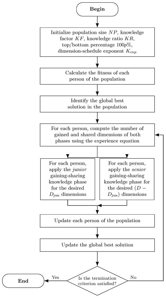
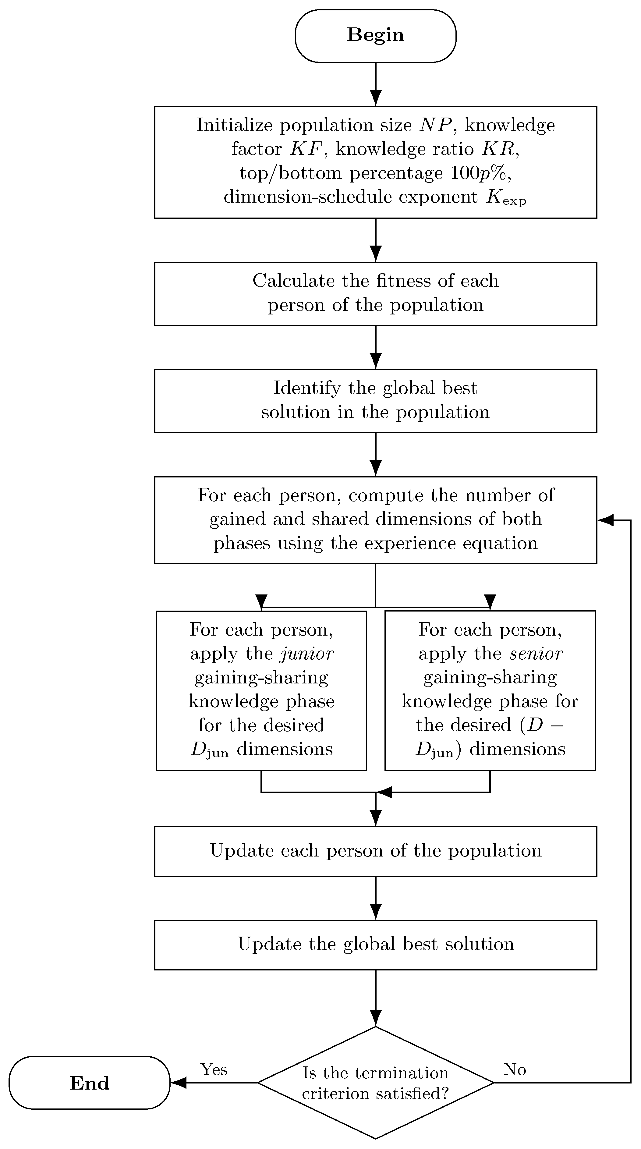
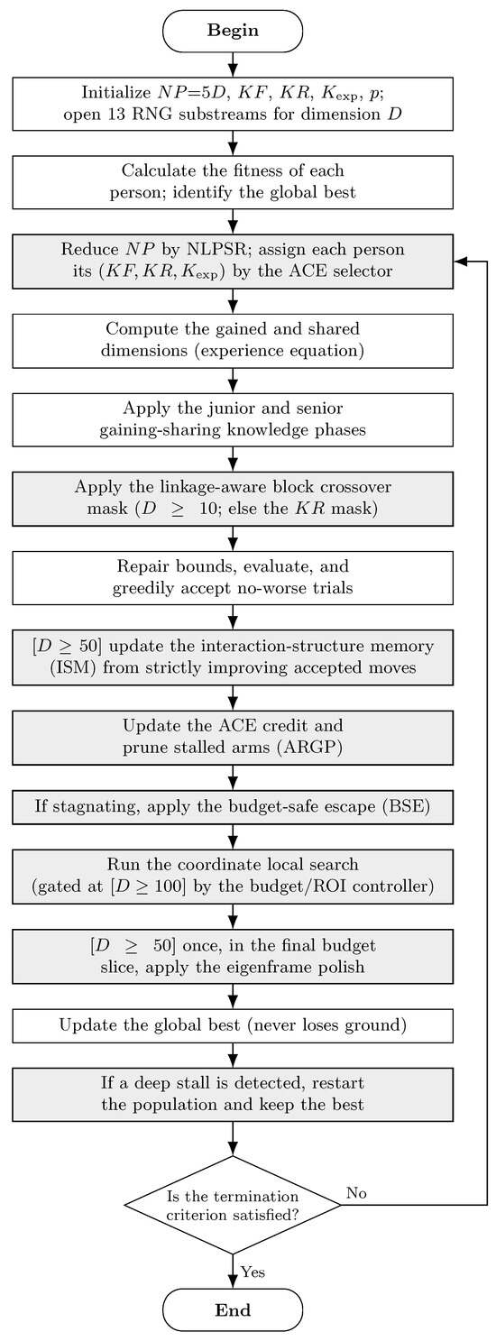
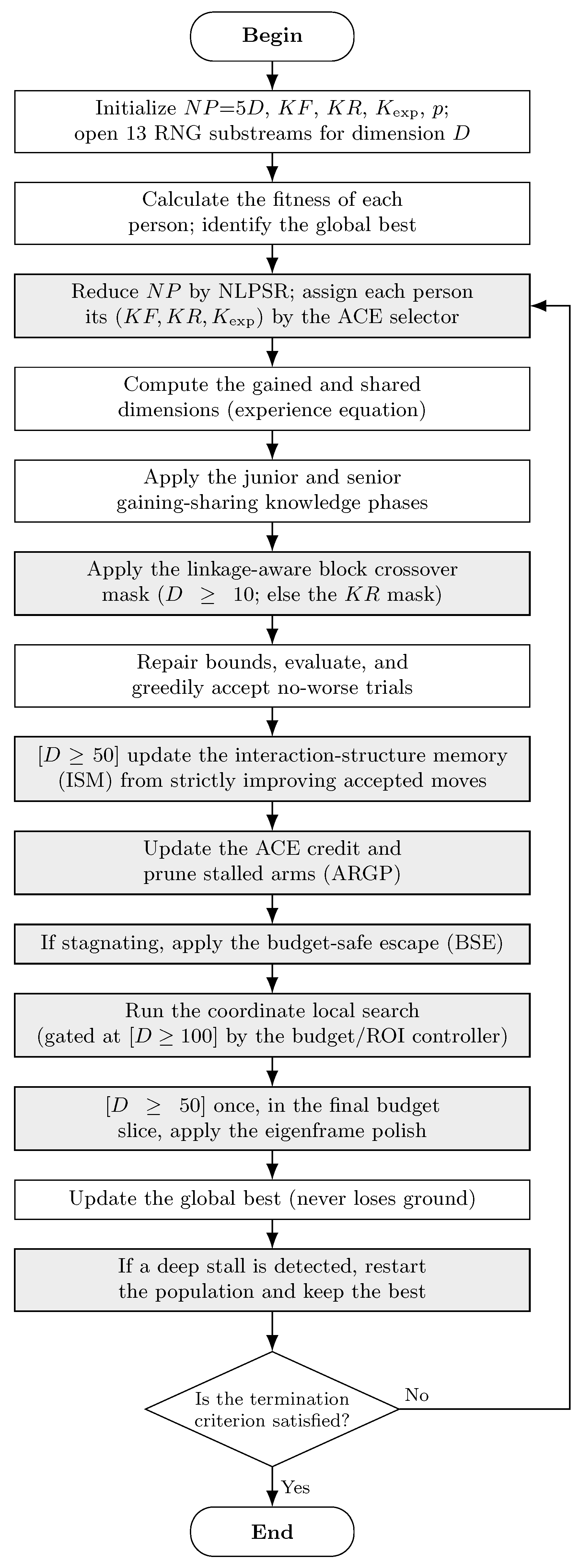
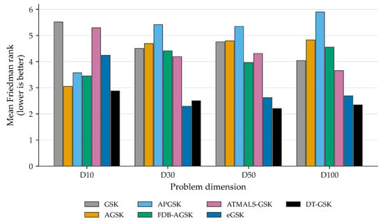
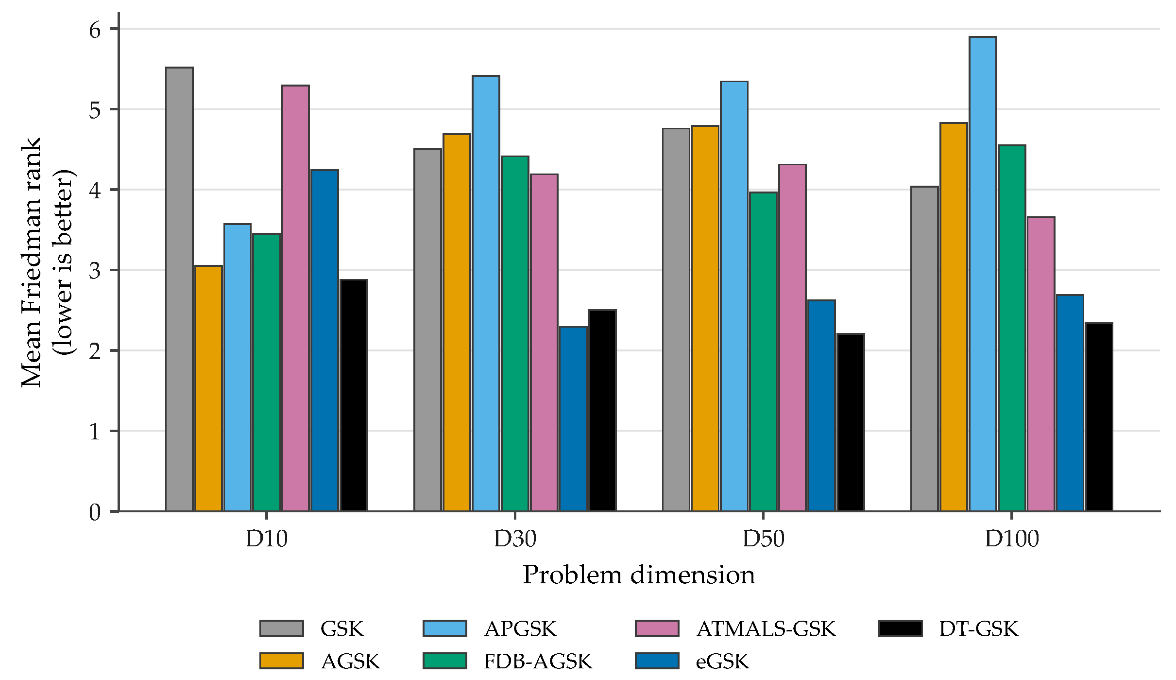
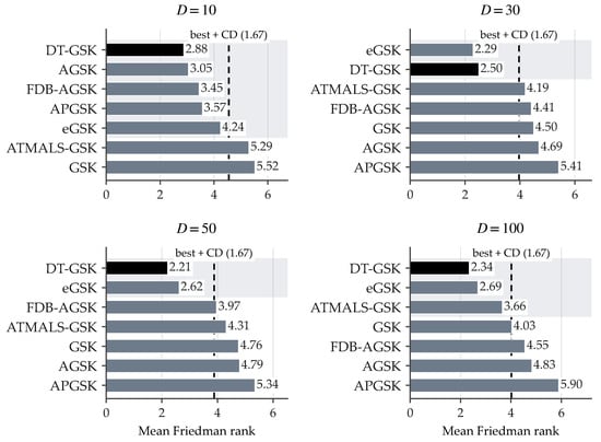
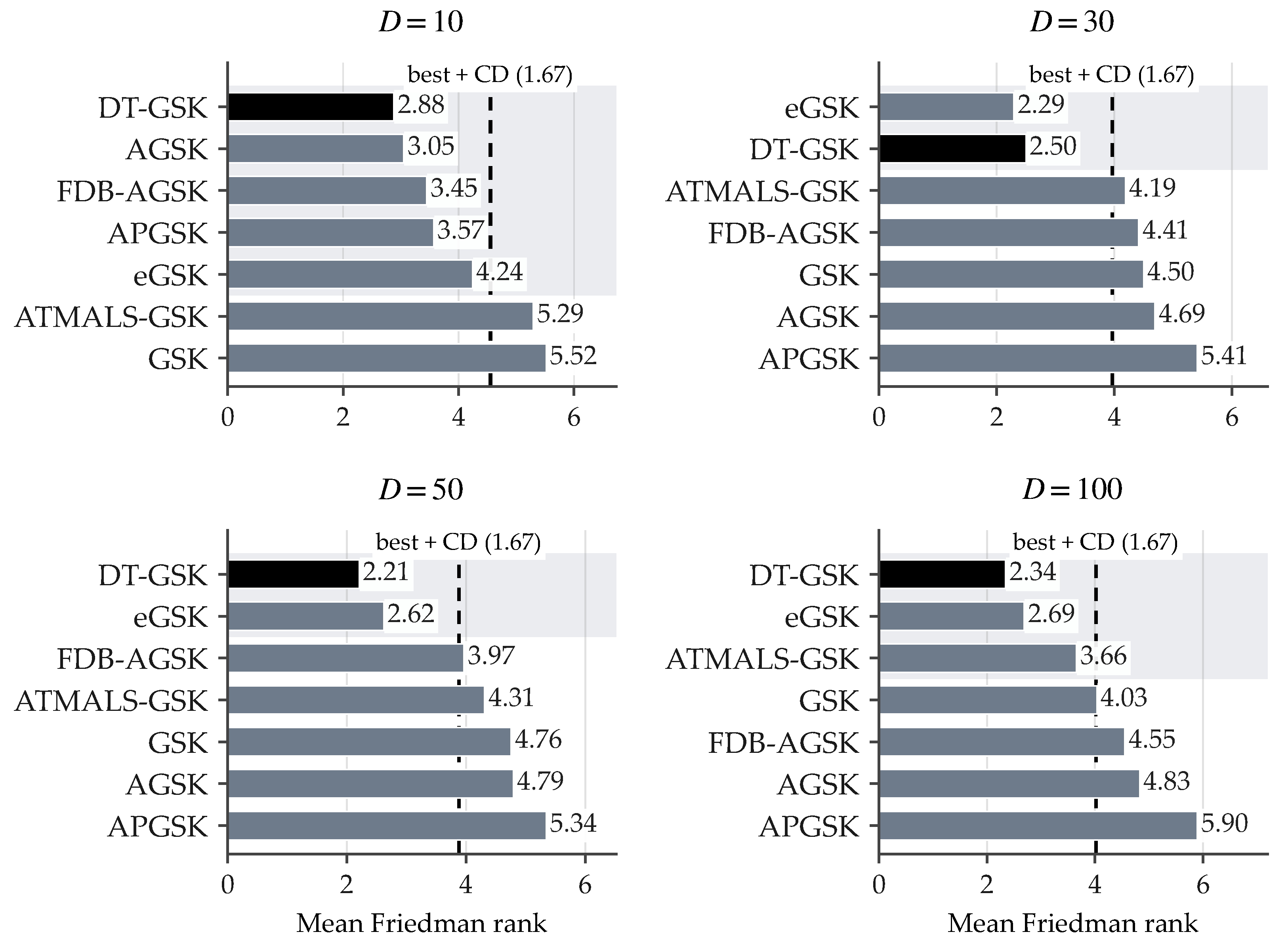
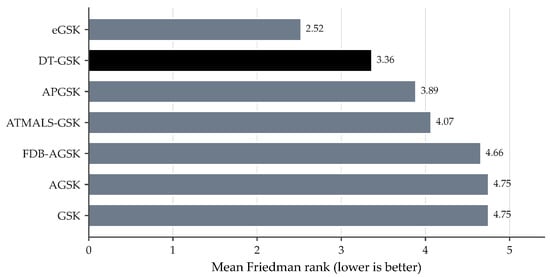
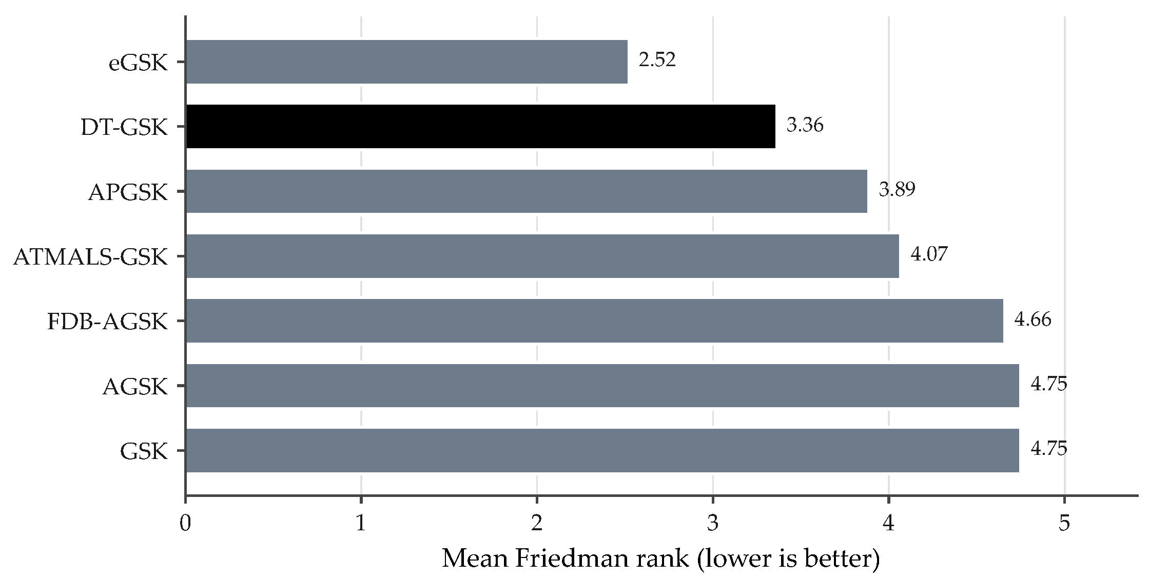
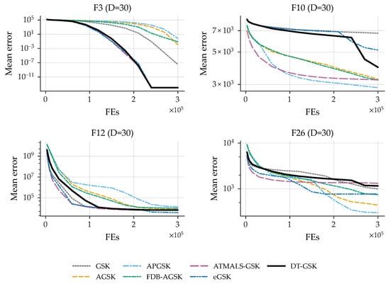
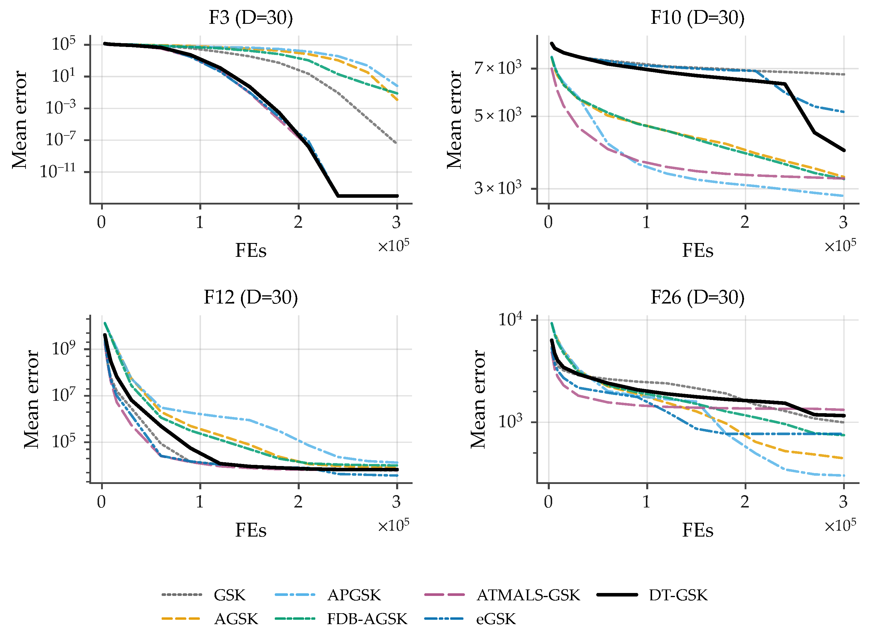
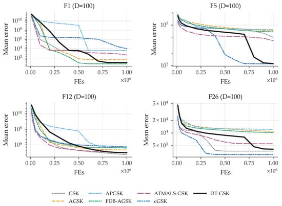
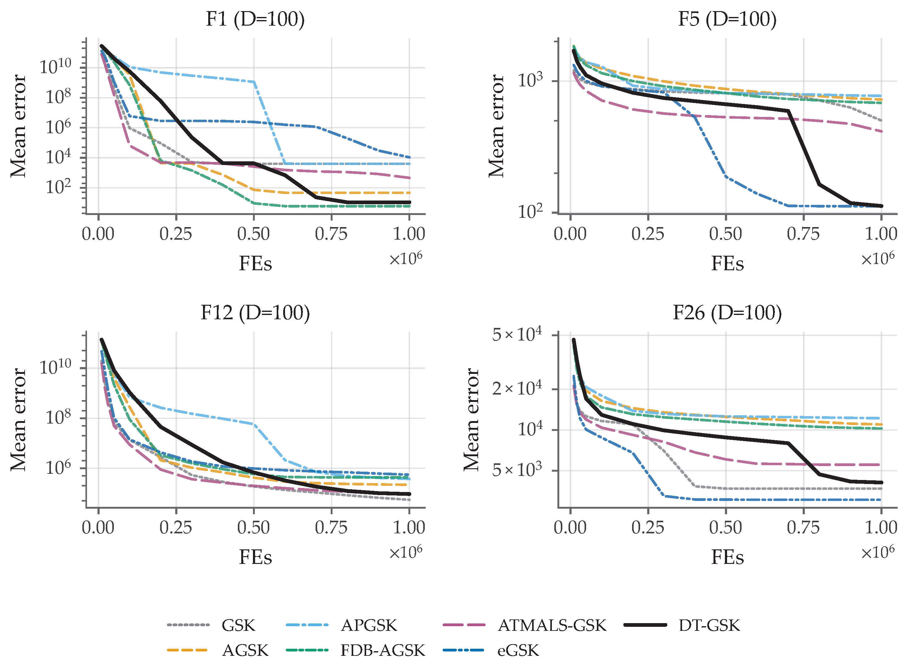

Disclaimer/Publisher’s Note: The statements, opinions and data contained in all publications are solely those of the individual author(s) and contributor(s) and not of MDPI and/or the editor(s). MDPI and/or the editor(s) disclaim responsibility for any injury to people or property resulting from any ideas, methods, instructions or products referred to in the content. |
© 2026 by the authors. Licensee MDPI, Basel, Switzerland. This article is an open access article distributed under the terms and conditions of the Creative Commons Attribution (CC BY) license.