


Abstract
Explainable artificial intelligence (XAI) is increasingly important in scientific and engineering applications where predictive performance alone is insufficient and model outputs must also be physically credible, transparent, and reliable under unseen conditions. This study proposes a domain-informed XAI framework for predicting total suction in xanthan gum-treated clays using 139 experimental observations covering different mineralogical, moisture, polymer-dosage, and curing conditions. Eleven linear, kernel-based, ensemble, boosting, and physics-guided algorithms were evaluated using leakage-resistant five-fold grouped cross-validation, including a matched constrained–unconstrained HGB comparison with identical model settings. The methodological contribution is an evidence-linked XAI validation protocol in which model explanations are not accepted from feature attribution alone, but are audited through their agreement with leakage-resistant grouped generalization, physically constrained response directions, matched experimental contrasts, residual behavior, predictive uncertainty, and applicability-domain support. Selective monotonic constraints, physics-guided residual learning, SHAP explanations, and nonlinear response visualization are integrated within this protocol as complementary sources of evidence rather than treated as independent indicators of interpretability. The unconstrained histogram–gradient-boosting model achieved the highest out-of-fold predictive performance (R2 = 0.958, RMSE = 0.098, and MAE = 0.070 in log10(MPa)). The corresponding monotonic model produced R2 = 0.935, RMSE = 0.121, and MAE = 0.094 but eliminated the directional violations detected in the unconstrained response, revealing a measurable trade-off between predictive accuracy and guaranteed physical consistency. Explanations identified moisture content as the dominant negative control and revealed that xanthan-gum effects were non-monotonic and dependent on curing, moisture, and mineralogy. The residual model remained interpretable but underperformed the leading ensembles. Overall, the framework validates explanations against experimental contrasts, physical directions, grouped generalization, residual behavior, uncertainty, and domain support, offering a transferable strategy for trustworthy XAI in structured scientific datasets.
1. Introduction
Artificial intelligence is now routinely used to construct predictive surrogates for complex physical systems, yet the scientific value of a model depends on more than numerical accuracy. In engineering applications, a prediction must be traceable to physically meaningful variables, stable under modest perturbations, and accompanied by evidence that the model has learned generalizable structure rather than artefacts of sampling or data leakage. These requirements have accelerated the development of explainable artificial intelligence (XAI), which seeks to make algorithmic behavior understandable through intrinsically interpretable models, post hoc attribution, local explanations, counterfactual reasoning, visual analytics, and formal evaluation of explanation quality [1,2,3,4,5,6,7,8]. XAI is particularly important for scientific machine learning because explanation is expected not only to support user trust, but also to reveal mechanisms, challenge implausible correlations, and guide subsequent experiments [9,10,11,12,13].
The literature distinguishes between interpretability, which concerns the transparency of a model or representation, and explainability, which concerns the generation of human-understandable accounts of model behavior [3,5,7]. Local methods explain individual predictions, whereas global methods summarize the response of a model over its domain. Model-agnostic approaches such as LIME approximate the decision surface around a selected observation [14], while SHAP uses cooperative-game-theoretic values to allocate a prediction among the contributing variables [15]. TreeSHAP enables efficient and theoretically consistent attribution for tree ensembles [16,17]. Partial-dependence plots, individual conditional expectation curves, and accumulated local effects provide complementary descriptions of nonlinear response structure [18,19,20]. Counterfactual explanations identify minimal input changes associated with alternative outcomes [21], and gradient-based methods such as Integrated Gradients and Grad-CAM have become central to deep-model interpretation [22,23]. Together, these methods have transformed explanation from an informal visual exercise into a diverse algorithmic research field.
Nevertheless, the existence of an explanation does not guarantee that it is faithful, robust, or scientifically meaningful. Explanation methods can be unstable under small input or model perturbations [24,25], can be manipulated by adversarial model constructions [26], and may assign importance to variables that are correlated rather than causally influential [27]. Sanity checks have shown that some saliency methods can remain visually plausible even when model parameters or labels are randomized [28]. Feature-removal benchmarks such as ROAR and related evaluation frameworks therefore emphasize the need to assess fidelity rather than relying on visual persuasiveness alone [29]. Rigorous XAI evaluation should consider correctness, completeness, consistency, stability, sparsity, human usability, and task relevance [6,8,30,31,32]. In high-stakes contexts, transparent models may be preferable to post hoc explanations of opaque predictors [12], whereas in scientific discovery, a hybrid strategy is often more appropriate: a high-performing model is retained, but its explanations are tested against governing physical expectations and independent diagnostic evidence.
Physics-informed machine learning provides a natural bridge between explanation and scientific credibility. Rather than treating observations as unconstrained numerical pairs, physics-informed approaches incorporate conservation laws, constitutive relationships, dimensional structure, monotonicity, symmetry, boundary conditions, or mechanistically motivated features during model design [33,34,35,36]. Physics-informed neural networks embed differential-equation residuals in the loss function [37], while process-guided and theory-guided architectures combine numerical models with data-driven correction [34,35,36]. In smaller tabular datasets, the same philosophy can be implemented through signed or monotonic constraints, physically transformed variables, residual learning around a mechanistic baseline, and explicit audits of response direction. Such approaches are attractive because they improve interpretability at the algorithmic level: the model is not merely explained after fitting; it is designed so that selected parts of its behavior conform to established knowledge.
Unsaturated soil mechanics provides a demanding test bed for physics-informed XAI. Soil suction governs water retention, hydraulic conductivity, effective stress, deformation, collapse, swelling, and shear strength [38,39,40,41,42,43]. Classical formulations by Brooks and Corey, van Genuchten, and Fredlund–Xing represent the soil-water retention curve using compact physically interpretable equations [44,45,46]. These models remain indispensable when complete drying or wetting paths and reliable residual and saturated water contents are available. However, they become difficult to calibrate independently when only sparse moisture states are observed for numerous treatment combinations. In such cases, a single curve can conceal mineralogical and treatment effects, whereas separate parameterization of every condition can be non-identifiable. A hybrid algorithmic formulation can retain the principal physical expectation—suction generally decreases with increasing water content—while learning nonlinear shifts associated with mineralogy, additives, and curing.
The present application concerns xanthan gum, a microbial biopolymer increasingly investigated as a lower-carbon soil modifier. Xanthan gum forms viscous hydrogels, coats particle surfaces, bridges grains, and modifies pore connectivity and water-film continuity. Previous studies have demonstrated substantial changes in strength, stiffness, erosion resistance, permeability, and fabric in biopolymer-treated soils [47,48,49,50,51,52]. The magnitude and even direction of these changes depend on soil mineralogy, polymer concentration, moisture condition, density, and curing. Clay minerals add further complexity because kaolinite and bentonite differ strongly in specific surface, diffuse-double-layer behavior, plasticity, and bound-water retention. Consequently, the effect of xanthan gum on total suction cannot be represented safely by a universal monotonic dosage rule. Early hydration can redistribute water and locally reduce suction, while longer curing can promote polymer-network development and increased water retention. This interaction makes the problem well suited to an XAI framework that separates dominant physical controls from treatment-dependent nonlinear deviations.
Machine-learning methods have been increasingly applied to soil-water and geotechnical prediction problems, including random forests, support-vector machines, gradient boosting, evolutionary regression, and neural networks [53,54,55,56,57,58]. Random forests and extremely randomized trees are effective for small nonlinear tabular datasets because they capture thresholds and interactions with limited preprocessing [53,54]. Gradient boosting and XGBoost iteratively construct additive tree ensembles [55,56], while CatBoost addresses prediction bias and categorical structure through ordered boosting [57]. Support-vector regression provides a kernel-based alternative for smooth nonlinear mapping [58]. Yet comparisons among such methods are frequently based on random train–test divisions. When repeated specimens or closely related experimental configurations are split across both sets, estimated performance can be severely optimistic. Cross-validation must reflect the data-generating hierarchy, and grouped or blocked validation is recommended whenever observations share sites, subjects, batches, spatial locations, or experimental configurations [59,60,61].
This concern is central to the current database because corresponding soil–xanthan-gum–moisture configurations occur at 1, 7, and 28 days. A conventional random split can place one curing-age variant in training and another closely related variant in testing, allowing the model to exploit repeated structure rather than generalize to an unseen experimental configuration. Accordingly, this study uses five-fold GroupKFold validation, in which all related curing-age observations remain within the same fold. Out-of-fold predictions are retained for every specimen and every algorithm, enabling model comparison, residual analysis, and explanation on genuinely held-out configurations. This design follows the broader principle that model selection and performance estimation should be separated and that validation units should match the intended domain of generalization [59,60,61,62].
A further challenge is that model accuracy and explanation quality can conflict. Highly flexible ensembles may outperform constrained models, but their predictions require post hoc interpretation. Conversely, aggressive physical constraints may improve plausibility while suppressing legitimate interactions. Recent work on Rashomon sets highlights that many near-optimal models can coexist and that interpretability may be a property of a region of model space rather than of a unique predictor [63]. For an engineering XAI study, it is therefore insufficient to declare a single winner based only on R2. Performance, residual bias, stability across folds, physical consistency, uncertainty calibration, and explanation coherence must be assessed together. Conformal and ensemble-based intervals further help distinguish interpolation from poorly supported extrapolation [64,65,66].
The methodological advance of this study does not lie in proposing a new attribution algorithm or predictive learner. Rather, it addresses a less developed problem in scientific XAI: how to determine whether a model explanation is sufficiently supported to be interpreted as physically meaningful. In many application studies, grouped validation, physical constraints, SHAP analysis, residual diagnostics, uncertainty estimation, and applicability-domain assessment are performed separately, if at all, and no explicit criterion connects these outputs. The proposed framework links them into an evidence chain in which an explanation is considered credible only when its direction and conditional behavior are consistent across held-out experimental groups, established physical expectations, matched laboratory contrasts, residual patterns, uncertainty levels, and local data support. This converts explainability from a post hoc visualization exercise into an auditable scientific validation process. The framework also distinguishes three outcomes that conventional SHAP-based analyses often conflate: an explanation that is physically and experimentally supported, an explanation that is model-faithful but weakly supported by the available domain, and an explanation that conflicts with observed or physically expected behavior [67]. The present study addresses this agenda through an algorithm-centered framework rather than a conventional materials-comparison paper. Its contribution is not merely the application of SHAP to a high-performing regressor. Instead, it combines four layers of explainability: (i) transparent experimental contrasts and matched treatment effects; (ii) physics-informed model construction through monotonic constraints and signed residual baselines; (iii) post hoc global and local explanations using SHAP and accumulated-response visualization; and (iv) explanation validation using grouped generalization, residual diagnostics, uncertainty, and applicability-domain analysis.
Accordingly, the objectives of this study are to (1) establish the independent physical effects of moisture content, mineralogical plasticity, xanthan-gum dosage, and curing on measured suction; (2) compare eleven linear, kernel, ensemble, and physics-informed algorithms under leakage-resistant grouped cross-validation, including a matched constrained–unconstrained HGB ablation; (3) quantify the predictive-accuracy and physical-consistency trade-off introduced by monotonic constraints and physics-guided residual learning; (4) interpret the selected models through SHAP, response surfaces, treatment-effect matrices, and a nine-panel algorithmic response atlas; (5) quantify residual structure and predictive uncertainty; and (6) provide a reader-oriented workflow that converts model explanations into material-screening and confirmatory-testing decisions. The central methodological contribution is therefore a reproducible explanation-auditing protocol that connects predictive validation, physical plausibility, experimental evidence, residual behavior, uncertainty, and domain support. This protocol provides an explicit basis for deciding when an explanation can be interpreted scientifically and when it should instead be treated as uncertain, extrapolative, or potentially misleading.
2. Materials and Database
2.1. Soil Systems and Variables
The experimental program was designed to span a deliberately broad mineralogical and plasticity domain rather than represent only a single clay. Three soil systems were selected: kaolinite (LL = 71%; PI = 38%), a 50:50 kaolinite–bentonite mixture (LL = 138%; PI = 104%), and bentonite (LL = 201%; PI = 164.5%). These materials represent progressively greater surface activity, diffuse-double-layer influence, and water-retention capacity. Kaolinite provides a comparatively low-activity reference dominated by relatively rigid 1:1 clay platelets, whereas bentonite represents a highly active smectitic system with large specific surface area and strong hydration potential. The 50:50 mixture supplies an intermediate fabric in which the contrasting mineralogical behaviors coexist. This three-level design therefore enables the models to distinguish treatment effects from the much larger baseline influence of clay mineralogy.
The selected input variables were liquid limit (LL), plasticity index (PI), xanthan-gum dosage (XG), measured gravimetric moisture content (MC), curing time, and void ratio. LL and PI were retained as practical proxies for mineral surface activity, bound-water demand, and the shape of the soil-water retention response. They were not interpreted as independent causal variables because both co-vary strongly with soil mineralogy. Void ratios of 1.54, 1.52, and 1.27 were assigned to kaolinite, the 50:50 mixture, and bentonite, respectively, and were included to represent differences in pore-space availability and packing state. The combination of LL, PI, and void ratio therefore encodes complementary information on mineralogy, plasticity, and pore structure, while MC, XG dosage, and curing time describe the imposed hydraulic and treatment conditions.
Xanthan gum was examined at 0, 0.5, 1.0, and 2.0% by dry soil mass. This range was selected to capture untreated behavior; low-to-moderate dosages commonly reported as effective for biopolymer stabilization; and a higher dosage at which polymer agglomeration, excess hydrogel formation, or trapped pore water may cause non-monotonic behavior. Curing periods of 1, 7, and 28 days were used to separate immediate hydration and mixing effects from progressive polymer redistribution, drying, particle bridging, and fabric reorganization. Because the actual water content after preparation and curing can depart from the nominal target, the measured MC was used in every physical and algorithmic analysis. This decision prevents the model from attributing suction changes to nominal treatment categories when they are actually caused by specimen-specific water loss or redistribution.
The complete database contains 139 observations. The balanced factorial core consists of 117 measurements distributed across the three soil systems, four XG levels, multiple moisture states, and three curing ages (See Table 1). Suction was modeled as log10(psiMPa), because the measured response spans almost two orders of magnitude, and the transformation reduces heteroscedasticity, limits domination by the highest-suction observations, and yields residuals that are more suitable for comparative algorithm assessment. The original suction values in MPa were nevertheless retained for physical interpretation and engineering use.
Table 1.
Summary of the experimental database and variable ranges.
2.2. Specimen Preparation and Curing
The kaolinite, bentonite, and 50:50 kaolinite–bentonite materials were first air-dried at ambient laboratory temperature, gently pulverized to break down agglomerates, and then passed through a 425 μm sieve to obtain a consistent fine-grained fraction. For each soil system, a fixed dry mass was selected to maintain a comparable specimen volume: approximately 31.5 g for kaolinite and the 50:50 mixture and 32.0 g for bentonite. This mass-controlled approach reduced variation in specimen geometry and supported consistent comparison across mineralogical groups.
Xanthan-gum powder was incorporated at 0, 0.5, 1.0, and 2.0% by dry soil mass. Because direct addition of xanthan gum to water can produce rapid hydration and localized agglomeration, the dry polymer was first blended thoroughly with the dry soil. Water was then added incrementally while the mixture was continuously folded and mixed until a visually uniform soil–polymer paste was obtained. Particular care was taken to break down any developing polymer-rich lumps and to distribute the hydrogel precursor uniformly throughout the specimen. The measured water content, rather than the nominal target content, was retained in the modeling database.
The prepared mixtures were placed into stainless-steel rings and compacted to a consistent specimen form. Each specimen was labeled according to soil type, xanthan-gum dosage, moisture condition, and intended curing age, and then sealed to minimize unintended moisture loss. Curing was carried out at approximately 20–25 °C for 1, 7, or 28 days. The sealed-storage procedure limited exposure to direct sunlight, air movement, and short-term temperature fluctuations, thereby allowing the measured changes in suction to be interpreted principally in relation to moisture state, mineralogy, polymer dosage, and curing time.
2.3. Total-Suction Measurement Using the WP4C Dewpoint Potentiometer
Total suction was measured using a WP4C Dewpoint PotentiaMeter (METER Group, Pullman, WA, USA). The instrument determines water potential from the equilibrium relative humidity of the vapor phase above a sealed soil specimen (See Figure 1). It combines a chilled-mirror dewpoint sensor with an infrared specimen-temperature sensor. During measurement, the mirror is cooled until condensation is first detected; the dewpoint temperature and specimen temperature are then used to determine equilibrium relative humidity and total water potential. Because the vapor-equilibrium method responds to both capillary and solute-related reductions in water chemical potential, the measured response represents total suction, incorporating matric and osmotic components [38,68].
Figure 1.
WP4C dewpoint potentiometer used for total-suction measurement, showing the digital display and the sample-chamber drawer.
The conversion from equilibrium relative humidity to total water potential follows the Kelvin relation:
where ψ is total water potential, R is the universal gas constant, T is absolute temperature, Vw is the partial molar volume of water, and RH is equilibrium relative humidity expressed as a decimal. Negative water potential was reported as a positive suction magnitude in MPa. The WP4C measurement range extends from approximately 0.1 to 300 MPa, which is appropriate for the broad suction domain encountered in fine-grained and bentonite-rich soils. The chilled-mirror approach is also recognized in ASTM D6836 for high-suction soil-water retention measurements [68].
ψ = (RT/Vw) ln(RH),
Before testing, the WP4C chamber and mirror were inspected and cleaned to prevent contamination. Calibration checks were performed using manufacturer-recommended standard salt solutions. A representative portion of each cured specimen was transferred into a clean stainless-steel sample cup, forming a shallow and approximately level surface while avoiding soil contact with the rim. The cup was inserted into the sealed measurement chamber, and the reading was accepted only after the instrument indicated stable vapor equilibrium. Laboratory temperature was kept as stable as practicable because small temperature gradients can materially affect dewpoint-based measurements.
The WP4C was selected because it provides rapid direct measurement over a suction range that is difficult to cover using tensiometers or pressure-plate methods alone. This capability was essential for the present database, in which measured suction ranged from low single-digit values to more than 100 MPa. The method is particularly suitable for evaluating xanthan gum-treated soils because polymer hydration, particle coating, pore narrowing, and mineral–water interactions can simultaneously modify capillary and adsorptive water retention. Accordingly, total suction was treated as the experimentally measured response used for both physical interpretation and machine-learning development.
2.4. Supplementary High-Plasticity Experimental Observations and Domain Separation
Twenty-two supplementary high-plasticity measurements were retained in the complete experimental database to extend the range of index properties and pore states. These observations occupy a substantially different domain from the balanced factorial matrix, with LL = 411–503%, PI = 350–450%, XG = 0%, MC = 30%, and a nominal one-day condition. Their inclusion increases the overall mineralogical and structural diversity of the database, but their design is not factorial with respect to XG dosage, moisture, and curing. Treating them as interchangeable with the 117 factorial observations would therefore allow the algorithms to associate extreme LL and PI values with a narrow moisture-treatment condition and could distort the estimated contribution of polymer dosage or curing.
For this reason, the supplementary subset was used primarily for applicability-domain and transferability analysis rather than for selecting the best predictive algorithm. The principal model comparison’s grouped cross-validation, residual diagnostics, and SHAP interpretation were based on the 117 factorial measurements, where the effects of soil system, XG, moisture, and curing were systematically represented. The supplementary observations were then examined relative to the feature ranges of the factorial database to determine whether they fell within interpolation space or required extrapolation. This separation provides a more stringent test of model credibility than pooling all observations into a single random split, because it explicitly distinguishes predictive accuracy within the designed experiment from transferability to a more extreme high-plasticity domain.
Domain separation is especially important for explainable AI. Feature-attribution methods can produce numerically plausible explanations even when a prediction is made far outside the training distribution. Accordingly, explanations generated for the factorial domain were not assumed to remain valid automatically for the supplementary high-plasticity soils. The supplementary subset was instead used to identify changes in feature leverage, prediction interval width, and proximity to the training envelope. This strategy allows the complete database to support broader interpretation while preventing out-of-domain observations from inflating performance estimates or creating misleading global feature rankings.
2.5. Quality-Control Considerations
Quality control was implemented at specimen, instrument, database, and validation levels. At the specimen level, soils were sieved to a common fine fraction, fixed dry masses were used, XG was dry-blended before water addition, and specimens were sealed during curing to reduce uncontrolled moisture loss. Each sample was identified by soil type, polymer dosage, moisture condition, and curing age so that traceability was maintained from preparation to WP4C measurement. The actual gravimetric MC was retained as the hydraulic state variable because even small differences in water content can cause large changes in suction, particularly in the low-moisture range.
At the instrument level, the WP4C chamber, mirror, and sample cups were inspected and cleaned before testing, and calibration checks were performed using manufacturer-recommended salt standards. Samples were placed below the cup rim with a shallow, level-exposed surface to promote representative vapor exchange and prevent contamination of the chamber. Readings were accepted only after stable vapor equilibrium was indicated. Laboratory temperature was kept as constant as practicable, because temperature gradients between the sample and dewpoint mirror can bias relative-humidity measurements and, therefore, the calculated total suction. Suspicious readings were rechecked against sample condition, cup cleanliness, and instrument stability before inclusion.
At the database level, units, categorical labels, and physically admissible ranges were checked before modeling. Suction was retained in MPa and transformed consistently as log10(MPa); no target-derived variables were used as model inputs. Duplicate-looking observations were not removed automatically, because repeated values can represent valid controls across curing ages; instead, their experimental relationship was handled through grouped validation. Missing or inconsistent records were reviewed against the experimental matrix rather than imputed without context. Feature ranges for the factorial and supplementary subsets were documented separately to make the applicability domain explicit.
At the validation level, all observations sharing the same soil–XG–nominal-moisture configuration were assigned to the same GroupKFold partition. This prevented corresponding 1-, 7-, and 28-day specimens, and repeated untreated controls, from being divided between training and validation sets. Performance was evaluated from out-of-fold predictions using R2, RMSE, MAE, bias, and residual dispersion. Physical checks were performed in parallel by examining the sign of the moisture response, the behavior across plasticity classes, the non-monotonicity of XG effects, and the stability of explanations across folds. These controls were necessary because a model can achieve high statistical accuracy while violating fundamental retention behavior or relying on leakage between closely related specimens.
3. Soil-Water Retention and Domain-Informed Formulation
3.1. Classical Retention Models
Table 2 compares the soil-water retention and hybrid modeling approaches. The van Genuchten retention model expresses effective saturation, Se, as Equation (2):
where h is pressure head, alpha is related to the inverse air-entry scale, n controls the breadth of the pore-size distribution, and m governs curve asymmetry. In classical use, effective saturation is calculated from saturated and residual water contents, and the fitted parameters describe a continuous drying or wetting path. The model is attractive because its parameters can be linked qualitatively to pore structure and it can be coupled with unsaturated hydraulic-conductivity functions. However, treatment-specific calibration requires sufficiently dense water-retention data over the near-saturated, transition, and residual zones. In the present experiment, each soil–XG-curing combination contains only a small number of discrete moisture states; unconstrained fitting of alpha, n, m, and residual water content to each combination would therefore be weakly identifiable and highly sensitive to individual observations.
Table 2.
Comparison of soil-water retention and hybrid modeling approaches.
The Fredlund–Xing formulation is particularly useful for high-suction soils because it represents water content as a logarithmic function of suction and includes a correction that approaches zero water content at an imposed limiting suction [2]. Its flexibility is advantageous for bentonite-rich materials and WP4C measurements extending into the multi-megapascal range. Nevertheless, this flexibility is accompanied by several correlated shape parameters. Brooks–Corey-type models provide a simpler power-law representation beyond an air-entry value, but their abrupt transition is less suitable when adsorption and broad pore-size distributions produce gradual curvature. These classical models were therefore treated as physical reference frameworks rather than forced as independent curve fits for every treatment cell.
The central physical expectation common to these retention formulations is that suction decreases as water content increases, although the gradient and curvature depend on mineralogy, pore structure, hysteresis, and chemical conditions. Higher plasticity and bentonite content generally shift the retention response toward higher suction at a comparable gravimetric moisture content because a larger fraction of water is adsorbed on mineral surfaces and retained within fine pores. XG can modify the curve through pore filling, hydrogel formation, altered vapor equilibrium, and redistribution of water films. Its effect is therefore expected to interact with moisture and curing rather than act as a simple constant offset. These observations guided the choice of monotonic constraints and nonlinear interaction terms used in the algorithmic framework.
3.2. Domain-Informed Strategies
Domain knowledge was incorporated through established soil-water retention behavior, directional constraints, and empirically motivated feature transformations rather than through governing differential equations or conservation laws. The approaches were intentionally complementary: monotonic boosting enforces selected response directions inside the learner; residual learning decomposes the prediction into a constrained physical baseline and a flexible correction; and feature engineering exposes dimensionless or interaction-type variables that approximate known retention mechanisms. No monotonic constraint was imposed on XG dosage or curing, because the experiments show that their effects depend on moisture state and mineralogy.
The term “domain-informed” applies specifically to the directional constraints, the signed baseline, and the physically motivated feature transformations derived from established soil-water behavior. SHAP analysis, response-surface visualization, residual diagnostics, uncertainty estimation, and applicability-domain assessment do not themselves incorporate physical knowledge; instead, they provide complementary explanation and validation layers. Residual learning is evaluated separately as a diagnostic benchmark and is not treated as part of the explanation of predictor effects.
To isolate the effect of monotonic regularization from the predictive capability of the HGB architecture, an unconstrained HGB model was added as a matched baseline. It used the same six predictors, maximum of 250 boosting iterations, learning rate of 0.04, maximum of 15 leaf nodes, minimum of five observations per leaf, L2 regularization of 0.2, random seed, and GroupKFold partitions as the monotonic HGB model. The two models therefore differed only in the application of the monotonic constraint vector [1, 1, 0, −1, 0, 0], corresponding respectively to LL, PI, XG dosage, actual MC, curing time, and void ratio.
Strategy 1 is a monotonic constrained boosting method. A histogram gradient-boosting regressor was constrained so that predicted log suction was non-increasing with measured MC and non-decreasing with LL and PI. The moisture constraint represents the most robust retention principle in the database. Positive LL and PI constraints encode the expectation that, at comparable hydraulic states, greater plasticity and mineral activity support stronger water retention. XG, curing time, and void ratio were left unconstrained because their marginal directions are not universal. The constrained learner was evaluated using the same grouped folds as the unconstrained algorithms, allowing any gain in physical consistency to be weighed directly against predictive error.
Strategy 2 is a physics-guided residual learning method. The response was decomposed into a physically signed baseline and a nonlinear residual. Consistent with the supplied implementation, the baseline used PI, negative MC, logarithmic curing, time, the XG-curing interaction, and PI normalized by water content. The transformed design matrix was fitted using non-negative least-squares, so the sign of the moisture term remained negative while the remaining baseline contributions were non-negative. This component represents the broad retention surface, whereas the residual learner captures local departures caused by mineral-specific fabric, XG agglomeration, thresholds, and interactions not represented in the baseline.
All fitted baseline coefficients were constrained to be non-negative after the moisture predictor had been transformed as -MC. After fitting the baseline, residuals were calculated as r = y − yphys. A random forest was trained to predict these residuals from the original variables, and the final prediction was obtained as = yphys + . This architecture differs from ordinary stacking because the first component is deliberately restricted to a physically interpretable trend. Residual magnitude and structure provide an additional diagnostic: small, pattern-free residuals indicate that the baseline captures most systematic behaviour, whereas structured residuals reveal missing interactions or local regimes.
The rationale for this decomposition was to test whether the broad directional response could be represented transparently by a constrained baseline while the random forest captured treatment-dependent departures. It was not assumed that this structure would necessarily improve accuracy or interpretability. Moreover, the residual diagnostics reported for the competing models are independent of this residual-learning architecture. Given its lower predictive performance, the approach is retained as a diagnostic benchmark of the limitations of the simplified baseline rather than as the preferred model.
Strategy 3 is a physics-guided feature engineering method. Candidate features included PI/(MC + 1), LL/(MC + 1), MC/LL, XG ln(tc + 1), XG/(MC + 1), and ln(tc + 1), where tc is curing time. The ratios PI/(MC + 1) and LL/(MC + 1) express water content relative to plasticity-related water demand; MC/LL provides a normalized wetness indicator; XG/(MC + 1) represents polymer dosage relative to available water; and XG ln(tc + 1) permits the polymer contribution to evolve with curing. These terms do not claim a unique constitutive law, but they provide the learner with variables that are closer to the governing physical interactions than isolated raw inputs.
3.3. Physical-Consistency and Plausibility Assessment
Physical consistency was assessed independently of conventional accuracy metrics. First, one-dimensional response checks were used to verify that predicted suction generally decreased with increasing MC over the factorial domain. Second, soil-specific response surfaces were inspected to confirm that the model preserved the observed ordering and curvature among kaolinite, the 50:50 mixture, and bentonite without generating abrupt nonphysical discontinuities. Third, the XG response was evaluated conditionally at fixed soil, moisture, and curing states rather than through a global monotonic assumption. This is essential because the measured treatment effects were slightly negative at early age in some configurations but positive after longer curing.
The constrained model was not assumed to be superior merely because it obeyed selected directions. A constraint can improve extrapolation but can also increase bias if the chosen physical rule is too strong or is applied to a correlated proxy. Therefore, physical plausibility, grouped out-of-fold error, residual bias, and explanation stability were considered together. The preferred model was the one that achieved an acceptable balance between these criteria rather than the model with the smallest error under an unconstrained random split.
The remaining algorithms were retained as unconstrained predictive benchmarks because they represent different learning architectures and do not provide an identical implementation of the HGB monotonicity mechanism. Consequently, the independent effect of monotonic regularization was inferred from the matched HGB pair rather than from cross-algorithm differences.
A matched monotonicity audit was additionally conducted for the constrained and unconstrained HGB models. After fitting each model to the laboratory database, LL, PI, and actual MC were varied individually across 51 equally spaced values spanning their observed ranges, while the remaining predictors were held at each of the 117 observed configurations. This produced 5850 adjacent comparisons per feature and model. A violation was recorded when predicted suction decreased with increasing LL or PI, or increased with increasing MC. The audit was intended to quantify the physical-consistency benefit obtained in exchange for any change in grouped predictive accuracy.
3.4. Interpretation of Classical and Algorithmic Response Surfaces
Classical retention curves and machine-learning response surfaces answer related but different questions. A calibrated van Genuchten or Fredlund–Xing curve describes the continuous hydraulic path of a defined material under a specified wetting or drying history. The algorithmic model instead estimates suction across changes in mineralogy, XG dosage, and curing, as well as moisture. Accordingly, the response atlas should be interpreted as a conditional prediction surface within the observed experimental design, not as a replacement for a complete constitutive SWRC obtained from dense path-specific measurements.
The benefit of the algorithmic representation is its ability to share information across treatment combinations and to reveal interactions that cannot be estimated reliably by fitting a separate multi-parameter retention curve to each sparse subset. The corresponding limitation is that predictions inherit the distribution and correlations of the training database. Response surfaces were therefore accompanied by uncertainty intervals, grouped validation, and applicability-domain checks. Predictions outside the factorial ranges of LL, PI, XG, MC, curing, or void ratio should be treated as screening estimates requiring confirmatory testing.
3.5. Residual Learning as a Diagnostic Benchmark
Residual learning was used not only as a predictive technique but also as a mechanism-discovery tool. When the physical baseline systematically underpredicts or overpredicts a particular soil–XG-curing regime, the residual model identifies where simple monotonic retention concepts are insufficient. In future extensions, SHAP values of the residual component can then be examined to determine whether the learned correction is associated primarily with moisture thresholds, high plasticity, polymer dosage or curing interactions. In the present study, residual structure was interpreted as evidence of unresolved processes rather than as undifferentiated statistical noise.
This interpretation remains cautious: residual patterns do not prove a specific microstructural mechanism. They identify combinations for which additional measurements, such as pore-size distribution, microscopy, hydraulic conductivity, or separate matric and osmotic suction, would be most informative. The physics-guided framework therefore links prediction with experimental planning by directing future tests toward regions where the current physical baseline is least adequate.
4. Algorithms and Validation
The algorithmic evaluation was designed as a single integrated protocol rather than a sequence of disconnected model comparisons. Eleven candidate approaches were examined: multiple linear regression (MLR), ridge regression, radial-basis-function support vector regression, random forest, extra trees, gradient boosting, XGBoost, CatBoost, monotonic histogram gradient boosting, unconstrained histogram gradient boosting, and a physics-guided residual random forest. The model set was intentionally heterogeneous. MLR and ridge regression quantified the extent to which the response could be represented by additive global effects; support vector regression tested a smooth kernel representation; bagged and boosted trees captured thresholds, interactions, and non-additive behavior; and the two physics-informed alternatives examined whether explicit directionality or decomposition around a physically signed baseline improved transfer to unseen experimental configurations. All models used the same six input variables and the same log-transformed suction target, ensuring that observed differences reflected algorithmic behavior rather than inconsistent preprocessing.
Hyperparameters were selected conservatively to match the small, structured nature of the database. Excessively deep trees, very large boosting rates, and aggressive feature expansion were avoided because these settings can fit specimen-level noise while appearing accurate under ordinary random splits. Tree ensembles were regularized through limits on leaf size, feature subsampling, or learning rate, whereas the linear and kernel models were scaled within pipelines. The physics-informed monotonic model imposed non-decreasing responses to LL and PI and a non-increasing response to actual moisture content, while leaving XG dosage, curing time, and void ratio unconstrained because their effects were demonstrably conditional. The residual-learning model first represented the physically expected global structure and subsequently fitted only the remaining discrepancy, so its nonlinear component was required to explain departures rather than relearn the full suction relation from scratch.
Five-fold GroupKFold validation formed the core of the evaluation. The grouping variable represented soil type, XG dosage, and nominal moisture state, so the 1-, 7-, and 28-day variants of an analogous configuration remained together in either training or validation. This design prevents curing-age counterparts and repeated untreated controls from being distributed across both sets, a leakage pathway that would otherwise allow the algorithm to interpolate between nearly identical specimens. Each observation received exactly one out-of-fold prediction from a model that had not been fitted to its experimental group, and final performance was calculated from the complete vector of pooled out-of-fold predictions. Consequently, the reported scores estimate generalization to unseen treatment configurations rather than the easier task of predicting random held-out rows from already represented combinations.
The grouped design was also used for uncertainty estimation and residual interpretation. Fold-level metrics were retained to expose ranking instability, because an algorithm that performs well on average may fail when a particular soil, dosage, or moisture regime is withheld. No target-derived transformation, imputed response, or global preprocessing statistic was allowed to incorporate validation information. For scaled models, transformations were fitted inside each training fold. This hierarchy-aware validation strategy is particularly important for explainable AI: explanations derived from an overoptimistic split can faithfully describe a model that has learned experimental duplication rather than transferable physical relationships.
All primary metrics were computed in log10(MPa), which reduces the dominance of the highest-suction dry specimens and makes relative prediction errors more comparable across the response range. Coefficient of determination quantified explained out-of-fold variance, RMSE penalized occasional large deviations, and MAE represented typical absolute error with lower sensitivity to extremes. Median absolute error, mean bias, and residual standard deviation were additionally retained in the prediction workbook. Residuals were defined as observed minus predicted response, such that positive values indicate underprediction. Interpretation was based on the joint evidence from these metrics rather than R2 alone; a preferred model was expected to combine high explained variance, low average error, limited systematic bias, stable fold ranking, and physically plausible response surfaces.
Because the response was modeled logarithmically, raw-MPa errors were also reconstructed for practical inspection. This back-transformation is nonlinear: equal log-scale deviations correspond to different MPa errors at low and high suction. Therefore, the log metrics were used for fair statistical comparison, whereas raw-scale observed-versus-predicted values were used to judge engineering magnitude. Residual diagnostics included residual-versus-fitted trends, distributional shape, calibration against the 1:1 line, soil- and curing-specific error patterns, and error concentration near the edges of the sampled domain.
Explainability and uncertainty were embedded in the same evaluation framework. SHAP values were calculated for the final tree ensemble to decompose each prediction into feature-specific contributions. Global mean absolute SHAP values quantified the average magnitude of influence; beeswarm distributions showed whether high or low feature values shifted suction upward or downward; and dependence plots were examined for thresholds, interaction signatures, and heterogeneous treatment effects. Correlations among SHAP contributions were also evaluated because LL, PI, and void ratio jointly encode mineralogy; the resulting explanations were therefore interpreted as model-conditional evidence, not as isolated causal effects. Physical-response maps and matched experimental contrasts were used to check whether the attribution patterns agreed with directly observed behavior.
Predictive uncertainty was approximated within each held-out fold from the distribution of individual-tree predictions. The lower and upper quantiles define an empirical ensemble interval that reflects model disagreement under the available data, although it does not include all sources of laboratory, sampling, or structural uncertainty. Interval coverage and mean width were reported together: high coverage with very wide bounds is uninformative, whereas narrow intervals with low coverage are overconfident. Applicability-domain assessment complemented these intervals by identifying whether a query occupied the balanced factorial domain or the supplementary high-plasticity region. The complete protocol thus evaluated accuracy, stability, explanation, physical consistency, residual structure, and uncertainty as mutually dependent properties of a trustworthy scientific algorithm.
For each predictor, , a normalized extrapolation distance was calculated as , where , , and were obtained exclusively from the 117 factorial observations. The overall extrapolation score was defined as . A record was classified as inside the factorial interpolation domain when , and as extrapolative when . This criterion provides an explicit quantitative flag and does not imply that every point inside the bounding ranges is equally well supported.
All 22 supplementary observations had Dext > 0 and were therefore classified as extrapolative. Their scores ranged from 1.615 to 2.323, confirming that they were substantially outside the factorial calibration domain.
5. Experimental and Physical Results
5.1. Moisture Content and Mineralogy
Figure 2, Figure 3 and Figure 4 show effect of moisture content on suction for different clays. Across the 117 factorial observations, actual moisture content was the strongest negative control on log-transformed total suction (Spearman ρ = −0.565). This relation reflects the progressive loss of capillary curvature and adsorptive demand as water content increases. The decline was nonlinear: the greatest suction gradient occurred between the dry and low-moisture states, whereas incremental changes became smaller with wetter conditions. Such curvature is expected when the governing retention mechanism transitions from strongly adsorbed and thin-film water toward a more continuous pore-water phase. The WP4C response therefore captures not merely a statistical inverse correlation but a fundamental change in the thermodynamic energy state of water within the treated soil.
Figure 2.
Moisture–suction response for kaolinite across XG dosage and curing time.
Figure 3.
Moisture–suction response for the 50:50 kaolinite–bentonite mixture.
Figure 4.
Moisture–suction response for bentonite.
Mineralogy shifted the elevation and shape of this moisture–suction relation. LL and PI each exhibited ρ = 0.435 with log suction because they distinguish the kaolinite, mixed, and bentonite systems, while void ratio showed an inverse coefficient of comparable magnitude because the assigned structural state covaried with soil type. Mean log suction increased from kaolinite to the 50:50 mixture and then bentonite: at 1 day, the respective means were 0.817, 1.050, and 1.244, increasing to 0.865, 1.136, and 1.411 at 28 days. Bentonite contains a larger active surface area and a stronger diffuse-double-layer contribution than kaolinite, allowing it to maintain high water potential deficits across a broader moisture range. The mixed soil displayed intermediate behavior but did not behave as a simple arithmetic average, indicating that fabric, interparticle association, and the connectivity of bentonite-rich domains influence the macroscopic retention response.
The dry controls produced the highest measured suctions and exerted substantial leverage on raw-scale statistics, but their inclusion is physically important because they anchor the high-energy end of the response domain. At increasing moisture, separation among the three soils remained visible, demonstrating that mineralogical effects were not restricted to the driest state. Nevertheless, LL, PI, and void ratio should not be interpreted as independent causal variables in this database: each is partly a descriptor of the same mineralogical grouping. For this reason, subsequent physical interpretation emphasizes soil-specific curves and matched treatment contrasts, while the XAI analysis is used to describe how the fitted algorithm distributes predictive credit among correlated descriptors.
5.2. Xanthan-Gum and Curing Effects
The XG effect was evaluated against the untreated specimen matched by soil, curing age, and nominal moisture level, thereby separating the polymer response from the much larger baseline influences of mineralogy and water content. At 1 day, mean changes in log suction were −0.074, −0.075, and −0.022 for 0.5, 1, and 2% XG, respectively. After 7 days, the corresponding effects became +0.022, +0.053, and +0.052, and after 28 days, they increased to +0.053, +0.086, and +0.123. The sign reversal is a central experimental result: XG dosage cannot be represented by a universal positive monotonic constraint over all curing conditions.
At an early age, the polymer remains highly hydrated and may redistribute water locally, increase the fraction of mobile or weakly bound water, or delay establishment of a stable polymer-clay fabric. These plausible mechanisms could reduce the vapor-pressure deficit measured by WP4C relative to the untreated control, particularly where polymer hydration changes the effective water state more strongly than pore confinement. With curing, dehydration, and progressive adsorption may promote gel contraction, particle coating, and bridging, while partial pore obstruction may increase the energetic cost of water removal. The increasingly positive treatment effect at later ages is consistent with transition from a water-rich viscous phase to a more developed soil–biopolymer network. Microstructural measurements would be required to verify these mechanisms directly.
The response nevertheless remained heterogeneous among soils and moisture states. Polymer efficiency depends on the available mineral surface, pore dimensions, initial water-to-polymer ratio, and whether the XG network forms discrete agglomerates or continuous bridges. In kaolinite, lower surface activity may limit adsorption but permit polymer films to dominate interparticle bonding; in bentonite, extensive surface area increases interaction opportunities but also creates stronger competition for water. At high moisture, the intrinsic moisture effect can mask the polymer contribution, whereas at low moisture, the same dosage can substantially alter film continuity and adsorptive retention. The strongest average increase occurred at 2% XG after 28 days, but the existence of local plateaus and reversals supports treatment-specific optimization rather than the assumption that increasing dosage always produces a proportionate suction increase (See Figure 5).
Figure 5.
Mean XG treatment effect relative to matched untreated controls.
5.3. Implications for Retention Modeling
The measured curves preserve the fundamental decrease in suction with increasing water content but exhibit treatment-dependent offsets, local changes in slope, and soil-specific curvature. A single van Genuchten, Fredlund–Xing, or Brooks–Corey relation fitted to all records would merge distinct mineralogical systems and implicitly treat XG dosage and curing as unexplained scatter. Conversely, fitting an independent multi-parameter retention curve to every soil–XG-curing subset would be underdetermined because each subset contains only a small number of moisture states and does not independently identify saturated water content, residual water content, and all shape parameters. Parameter values could then appear physically meaningful while being controlled largely by the assumed bounds and initial guesses.
The appropriate interpretation is hierarchical. Classical retention theory supplies the dominant moisture-controlled backbone and establishes physically credible directionality. Mineralogy changes the baseline retention capacity and air-entry behavior; XG and curing then shift or reshape that backbone through changes in water binding, pore connectivity, and fabric. The physics-informed algorithms operationalize this hierarchy without claiming that machine-learning surfaces are complete constitutive SWRCs. Their outputs should be understood as conditional total-suction estimates within the tested ranges, not as full wetting–drying paths or direct substitutes for independently calibrated hydraulic functions.
Total suction measured by WP4C includes both matric and osmotic contributions. Although the specimens did not contain deliberately added salts, polymer hydration, dissolved constituents, and mineral surface chemistry can influence water activity. Consequently, differences among treatments cannot be attributed exclusively to capillarity. The observed response is best described as a coupled thermodynamic outcome of pore geometry, adsorptive surface forces, and solution effects. This distinction is important when linking the results to numerical unsaturated-soil models, which often require matric suction or a water-retention function coupled to hydraulic conductivity. Future work should therefore pair WP4C total-suction measurements with independent matric-suction techniques or pore-fluid characterization to resolve these components.
5.4. Multivariate Dependence and Coupled Physical Controls
The experimental response cannot be interpreted from isolated one-variable trends, because LL, PI, mineralogy, void ratio, moisture, and curing are structurally coupled. The Spearman matrix (Figure 6) provides a compact representation of these dependencies. Moisture exhibits the dominant negative relation with suction, whereas LL and PI act as mineralogical proxies. The matrix also demonstrates why ordinary partial regression coefficients can be unstable: LL, PI, and void ratio jointly encode soil type. Consequently, physical interpretation was based on matched treatment effects and soil-specific response surfaces rather than on marginal correlations alone.
Figure 6.
Spearman correlation structure of inputs and measured log suction.
The dependence structure also has direct implications for XAI. When correlated features are available to a flexible model, predictive contribution can be distributed among them in several statistically equivalent ways. A high SHAP magnitude for PI, for example, does not prove that PI alone causes the predicted change; it may represent a portion of the broader mineralogical contrast jointly encoded by LL and void ratio. Agreement between the correlation matrix, matched experimental contrasts, response surfaces, and SHAP direction is therefore more informative than any isolated ranking. This triangulation forms the basis of the physical interpretation adopted in the paper.
5.5. Curing Trajectories and Treatment-Response Matrix
Configuration-level trajectories reveal that curing does not produce a uniform vertical shift in suction. The direction and magnitude depend on mineralogy, moisture state, and XG dosage. Figure 7 overlays individual soil–dosage–moisture trajectories with dosage-level means, while Figure 8 expresses the average response relative to untreated controls. This representation separates the polymer contribution from the much larger baseline effect of water content and prevents an apparently strong soil effect from being misinterpreted as a treatment effect.
Figure 7.
Configuration-level curing trajectories and dosage-level mean responses.
Figure 8.
Curing-dependent treatment-response matrix relative to untreated controls.
Individual trajectories are especially valuable because averaging across moisture states can conceal opposing mechanisms. A positive dosage-level mean may coexist with local decreases at wetter conditions, while a nearly neutral mean may result from substantial positive and negative responses canceling each other. The trajectory plot therefore provides a visual test of treatment stability: parallel trajectories suggest a systematic curing effect, whereas crossings indicate interaction among curing, XG and moisture. The observed crossings justify retaining these interactions in the learning algorithms and explain why a purely additive linear model leaves structured residuals.
5.6. Nonlinear Physical Response Surfaces
The fitted response surfaces in Figure 9 visualize the joint XG–moisture influence at 28 days for the three soil systems. The surfaces are not presented as substitutes for direct measurements; instead, they expose the nonlinear structure learned from the complete factorial matrix. Steep gradients occur along the moisture axis, while the polymer axis shows soil-specific curvature and local plateaus. This confirms that a globally monotonic XG constraint would be physically over-restrictive, whereas the moisture constraint remains defensible.
Figure 9.
Three-dimensional algorithmic response surfaces at 28-day curing.
The nine-panel atlas extends this analysis across all curing ages and reveals how the response topology evolves with time. The dominant color transition remains aligned with the moisture axis, confirming that water state controls the first-order response. By contrast, the XG-related contours are relatively shallow at 1 day and become more differentiated at later ages, particularly in the mixed and bentonite systems. Local contour bending identifies regimes where XG modifies moisture sensitivity rather than simply adding a constant suction offset. These surfaces are useful for hypothesis generation, but interpretation should remain within the convex region supported by observations because tree ensembles can create visually smooth plateaus in sparsely sampled areas.
6. Algorithmic Results
6.1. Predictive Performance
The matched HGB comparison changed the interpretation of the model ranking (See Table 3). The unconstrained HGB achieved the highest grouped out-of-fold accuracy, with R2 = 0.958, RMSE = 0.098, and MAE = 0.070. Applying the monotonic constraints reduced R2 to 0.935 and increased RMSE and MAE to 0.121 and 0.094, respectively. Thus, the strong performance previously attributed to the physics-informed HGB model partly reflected the capability of the underlying HGB architecture, while the constraints imposed a modest but measurable predictive penalty.
Table 3.
Grouped out-of-fold predictive performance. Values in parentheses represent the standard deviations of the corresponding fold-specific metrics across the five validation folds.
The physical-consistency audit, however, demonstrated the benefit obtained from this reduction in accuracy (See Table 4). The unconstrained HGB violated the expected negative MC direction in 15.06% of the perturbation comparisons and showed a small LL violation rate of 0.15%, whereas no PI violations were detected. The monotonic HGB produced zero violations for all three constrained predictors. Accordingly, the constrained model should not be described as the most accurate predictor; its value is that it provides guaranteed directional consistency while retaining high grouped predictive performance.
Table 4.
Directional-violation rates obtained from one-variable monotonicity perturbation tests.
The comparative ranking was based exclusively on the reproducible out-of-fold predictions supplied with the analysis package. All subsequent performance statements, figures, and interpretation use this single final result set.
The performance gain of the leading ensembles was driven mainly by lower errors in the intermediate- and high-suction regimes, where the relation among moisture, plasticity, and dosage changes slope (See Figure 10 and Figure 11). Bagged trees are well suited to this structure because they partition the predictor space into locally homogeneous regions without requiring a single global functional form. Boosting methods also captured these interactions, but their sequential fitting made them more sensitive to hyperparameter choice and to difficult held-out groups. The ranking therefore reflects both representational capacity and robustness under the available sample size. The results should not be interpreted as evidence that random forest is intrinsically the best suction model for all datasets; they show that tree ensembles provide an effective bias–variance compromise for this particular structured experimental design.
Figure 10.
Grouped out-of-fold RMSE for the evaluated algorithms.
Figure 11.
Observed versus grouped out-of-fold random-forest predictions.
Fold-level results revealed that aggregate metrics alone conceal meaningful variation. Some validation folds withheld combinations concentrated at the dry or highly plastic edge of the design, producing larger errors for every algorithm. The leading models nevertheless retained comparatively stable ranks, whereas several boosted and residual models changed position depending on which treatment configurations were absent from training. This stability is an important criterion for scientific deployment: an algorithm that attains a high pooled R2 through exceptional performance in easy folds but fails on a physically distinct group is less dependable than a model with slightly lower average accuracy and consistent behavior.
6.2. Physics-Informed and Residual-Learning Comparison
The physics-guided residual random forest achieved R2 = 0.813, RMSE = 0.206, and MAE = 0.109 and therefore performed substantially worse than the leading direct ensemble models. Accordingly, it is not proposed as the preferred predictive approach. Its practical value is diagnostic: the result shows that the simplified physically signed baseline did not adequately represent the mineralogical and treatment-dependent curvature, leaving a difficult and noisy correction for the residual learner. The model is therefore retained as evidence of the limitations of this decomposition rather than as a major performance contribution.
The unconstrained HGB model achieved the highest grouped out-of-fold R2, while the monotonic HGB remained within the leading performance tier and provided guaranteed directional consistency. Its success indicates that the strongest directional assumptions—suction decreasing with actual moisture and increasing with plasticity descriptors—are compatible with the dominant experimental structure. Importantly, XG and curing were not constrained. A universal positive XG constraint would have contradicted the observed early-age reductions. This selective use of constraints is a central methodological finding: physics-informed learning benefits from encoding only relationships that are theoretically robust and empirically supported over the sampled domain.
The comparison also shows why physics-informed methods should be evaluated against unconstrained benchmarks rather than assumed to be superior. Constraints can reduce variance and prevent implausible extrapolation, but they can also introduce bias when predictors are correlated or when the measured response combines several physical components. The most defensible workflow is therefore dual: use the unconstrained ensemble to identify the attainable predictive ceiling, use the constrained model to test whether comparable accuracy can be achieved with stronger directional guarantees, and inspect disagreements as evidence of regions where the physical assumptions or data coverage require further investigation.
6.3. Residual Diagnostics
According to Figure 12 and Figure 13, the out-of-fold residuals of the leading ensembles were centered close to zero and did not display a strong global linear trend with fitted value, indicating limited overall bias. Nevertheless, residual variance was not completely constant. Dispersion increased near the dry, high-suction end of the response and in the most plastic bentonite configurations, where a small difference in water state produces a comparatively large change in total suction. This heteroscedastic pattern is physically plausible and suggests that a constant-variance Gaussian error model would be inadequate for uncertainty quantification across the entire domain.
Figure 12.
Residuals versus grouped out-of-fold fitted values.
Figure 13.
Distribution of grouped out-of-fold residuals.
The residual distribution was broadly symmetric but heavier-tailed than a normal distribution. A small number of group-held-out cases contributed disproportionately to RMSE while having less influence on MAE, justifying the joint reporting of both metrics. Soil-specific inspection showed that bentonite generated the largest positive and negative residuals, whereas kaolinite predictions were generally more compact. Curing-specific residuals did not indicate a simple systematic bias, which supports the inclusion of curing as an interacting predictor rather than as a uniform correction factor.
Residual analysis was also used as a diagnostic of missing physics. Clusters of positive residuals indicate regimes where the model underestimates measured suction and may be omitting stronger-than-expected adsorption, gel contraction, or pore blocking. Negative clusters indicate overprediction and may correspond to polymer-rich water states or local fabric conditions that weaken the assumed retention enhancement. These hypotheses are not proven by residuals alone, but they provide a rational basis for targeted follow-up measurements such as separate matric and osmotic suction, pore-size distribution, hydraulic conductivity, and microscopy.
6.4. Explainable AI
Although the unconstrained HGB model achieved the highest out-of-fold R2 and lowest MAE, random forest was retained as the post hoc explanation model because it achieved competitive predictive performance and permitted efficient TreeSHAP computation. Accordingly, the SHAP results describe the random-forest representation of the response surface rather than the unconstrained or constrained HGB models (See Figure 14). SHAP analysis identified actual moisture content as the dominant predictor, and high moisture values consistently produced negative contributions to predicted log suction. This direction agrees with both classical retention theory and the measured soil-specific curves, providing a first level of explanation validation. PI and LL carried much of the mineralogical contrast, while void ratio shared part of the same signal because it was fixed within soil groups. Curing time and XG showed smaller global mean absolute contributions, but their local effects were strongly heterogeneous. A low global rank therefore does not imply physical irrelevance; it indicates that the variable is influential only within particular combinations rather than across every record.
Figure 14.
Global mean absolute SHAP values for the random-forest explanation model. Error bars represent ±1 standard deviation across the 117 factorial observations.
The beeswarm and dependence patterns revealed that XG contributions changed sign with curing and moisture (See Figure 15). At early age or high water content, added XG could shift the prediction downward relative to the baseline, whereas after extended curing and at lower moisture, it increasingly shifted predictions upward. This pattern mirrors the matched experimental treatment effects and is one of the strongest pieces of evidence that the explanations are capturing a real interaction rather than an arbitrary model artefact. The response also demonstrates why reporting only a global feature-importance bar would be insufficient: averaging positive and negative local effects can make a mechanistically important variable appear weak.
Figure 15.
SHAP beeswarm plot showing the direction and heterogeneity of feature contributions for random-forest explanation model.
LL and PI were perfectly correlated in the present database (r = 1.000), while void ratio was strongly correlated with LL and PI (r = −0.889 and −0.886, respectively). These variables largely encode the same three-level mineralogical contrast, and their SHAP values should therefore not be interpreted as independent causal contributions. Instead, they were interpreted collectively as a mineralogical–structural descriptor block distinguishing kaolinite, the 50:50 mixture, and bentonite. The allocation of importance among these correlated predictors is model-dependent, whereas their combined contribution is more meaningful than their individual rankings.
The standardized MLR coefficients broadly supported the SHAP interpretation. Actual MC had the largest coefficient magnitude (−0.453), followed by PI (0.194) and LL (0.191), confirming that moisture and the combined mineralogical descriptors dominate the response. The random-forest SHAP analysis also ranked actual MC first but assigned greater importance to void ratio, reflecting its use in nonlinear partitions and its strong association with soil type. The comparatively good MLR performance therefore indicates a strong global linear structure, while the improved ensemble performance and response surfaces show that local thresholds and interactions remain important.
6.5. Predictive Uncertainty
The empirical 80% tree-ensemble interval covered 61.5% of held-out observations and had a mean width of 0.305 log units. Coverage was therefore substantially below the nominal 80% level, confirming that dispersion among individual trees is not a fully calibrated predictive distribution. Individual trees share the same training data and model family, so their spread reflects algorithmic disagreement but omits specimen variability, WP4C measurement uncertainty, uncertainty in moisture content, and structural error common to the ensemble (See Figure 16). The resulting bounds should therefore be described as empirical model-disagreement intervals rather than formal confidence or prediction intervals. Accordingly, no claim of calibrated 80% predictive coverage is made, and the 61.5% result is reported explicitly as evidence of under-coverage.
Figure 16.
Approximate ensemble uncertainty for grouped out-of-fold predictions.
Despite this limitation, interval width contained useful information. Wider bounds occurred disproportionately in high-suction, high-plasticity, and sparsely represented regimes, where held-out predictions depend on extrapolation across larger gaps in the factorial matrix. Narrower bounds were obtained in the densely supported middle of the moisture range. The interval pattern therefore acts as a local data-support indicator and complements the global applicability-domain analysis. A prediction with a plausible mean but a wide interval should trigger confirmatory WP4C testing rather than be accepted as a precise design value.
Future probabilistic development should use methods with explicit coverage guarantees, such as grouped conformal prediction, quantile regression forests, or distributional boosting. Importantly, calibration must preserve the same experimental grouping used for model validation; ordinary random conformal splits would again risk leakage among curing counterparts. Replicate laboratory testing would also permit decomposition of irreducible experimental variability from epistemic model uncertainty. Until such data are available, uncertainty reporting in this study is deliberately conservative and linked to a reader-oriented decision framework.
6.6. Multi-Criteria Model Ranking and Fold Stability
Figure 17 compares fold-level ranks across the evaluated algorithms. The unconstrained HGB, monotonic HGB, and random forest generally occupied the leading performance region, although their order varied among folds. This variability shows that model ranking depends partly on the held-out experimental configurations and supports interpreting aggregate metrics together with fold-level variability.
Figure 17.
Algorithm-rank stability across grouped cross-validation folds.
For interpolation within the tested factorial domain, the unconstrained HGB model may be preferred when minimizing average errors is the primary objective. For screening beyond densely sampled combinations, the monotonic model offers an additional safeguard against moisture or plasticity responses that violate the strongest physical expectations. The fold-stability plot makes this trade-off explicit by treating predictive performance as a vector rather than a scalar. Such multi-criteria selection is particularly appropriate for XAI applications, where explanation quality and physical consistency can be as consequential as a marginal difference in RMSE.
6.7. Residual Structure, Calibration, and Uncertainty
The four-panel diagnostic in Figure 18 combines residual-versus-prediction behavior, distributional shape, a normal quantile comparison, and observed–predicted calibration. Residuals remain centered near zero without a dominant global trend, although the tails are wider in sparse high-suction regions. Figure 19 orders the uncertainty intervals across the response domain. Wider intervals identify combinations where the model is extrapolating between relatively isolated configurations and should therefore be supplemented by confirmatory testing.
Figure 18.
Integrated residual, distribution, and calibration diagnostics for the monotonic HGB model.
Figure 19.
Empirical tree ensemble model disagreement intervals for the random-forest model across the measured response domain.
The calibration panel also shows that the ensembles reproduce the overall response range without severe compression toward the mean, a common weakness of small-data regressors. Some regression to the mean remains at the highest observed suctions, where predictions are slightly conservative. This behavior is preferable to uncontrolled overestimation but should be recognized when the model is used to screen very dry bentonite-rich specimens. The combined diagnostic supports the conclusion that error is dominated by local domain difficulty rather than a single global misspecification.
6.8. Feature-Contribution Dependence and Response Atlas
SHAP effects are additive at the prediction level but remain statistically dependent because the physical variables are coupled. Figure 20 maps correlations between feature contributions, helping distinguish independent importance from shared mineralogical information. Figure 21 provides a nine-panel atlas spanning three soils and three curing ages. The atlas is intended as an interpretable design-screening tool: readers can locate a soil system, curing age, XG dosage, and moisture state, and then assess the predicted suction regime and the steepness of nearby gradients.
Figure 20.
Dependence structure among SHAP feature contributions for the random-forest explanation model.
Figure 21.
Nine-panel response atlas across soil systems and curing ages.
The atlas reveals that the most persistent gradient is vertical, along the moisture axis, while horizontal XG gradients strengthen with curing and vary among soils. This topology is consistent with the SHAP evidence: moisture has a large, directionally stable effect, whereas XG exerts a conditional influence that depends on the surrounding state. The agreement among the atlas, matched treatment-effect matrix, and local SHAP contributions increases confidence that the model has learned a coherent representation of the experiment. Areas with flat, block-like contours should be interpreted cautiously because they may reflect tree partitioning and limited resolution rather than a truly discontinuous physical process.
6.9. Limitations and Future Research
Despite the strong predictive performance and the physically informed structure of the proposed framework, several limitations should be acknowledged. First, the database contains 139 observations, and although this is sufficient for comparative modeling under grouped cross-validation, it remains relatively small for developing highly flexible machine-learning models. The limited sample size may increase sensitivity to individual experimental groups and may restrict the stability of model rankings across alternative validation partitions. The reported results should therefore be interpreted as evidence of performance within the investigated experimental domain rather than as definitive proof of universal generalization.
Second, the experimental database is structured around a limited number of soil systems, namely kaolinite, a 50:50 kaolinite–bentonite mixture, and bentonite. Liquid limit, plasticity index, and void ratio are consequently strongly associated with soil type and are not independently varied. Although these variables provide useful numerical descriptors of mineralogical and structural differences, their individual SHAP contributions should not be interpreted as independent causal effects. In particular, the model may distribute predictive importance among LL, PI, and void ratio in different ways because these variables partially encode the same underlying mineralogical contrast. A broader database containing soils with independently varying mineralogy, plasticity, density, and pore structure would be required to separate these effects more rigorously.
Third, the xanthan gum-dosage, moisture-content, and curing-time ranges are limited to the experimental conditions considered in this study. The model was developed using XG contents of 0–2%, curing periods of 1–28 days, and the measured moisture-content range represented in the database. Predictions outside these intervals represent extrapolation and should not be used directly for engineering design without confirmatory laboratory testing. This limitation is particularly important for very high polymer dosages, extended curing periods, wetting–drying cycles, or near-saturated conditions, where additional mechanisms such as biodegradation, polymer redistribution, cracking, hysteresis, and long-term fabric evolution may become important.
Fourth, total suction was measured using the WP4C dewpoint potentiometer. This method provides an efficient measure of total suction over a broad high-suction range; however, it does not separately quantify matric and osmotic suction. Xanthan gum may affect both components through pore-scale water retention, dissolved polymer effects, ion interactions, and changes in vapor equilibrium. Consequently, the present model predicts total suction but cannot determine whether an observed change is caused primarily by capillary, adsorptive, or osmotic mechanisms. Future studies should combine WP4C measurements with methods capable of independently characterizing matric suction, pore-water chemistry, electrical conductivity, and osmotic effects.
Fifth, the grouped validation strategy reduces leakage between closely related soil–treatment–moisture configurations, but it does not fully replicate validation against an entirely independent experimental campaign. All observations were generated within the same overall laboratory program, using similar preparation procedures, equipment, and environmental conditions. Therefore, unrecognized laboratory-specific characteristics may still be shared across the training and validation folds. External validation using specimens prepared by different operators, laboratories, soil sources, and xanthan-gum products would provide a more demanding test of model transferability.
Sixth, the monotonic constraints imposed on moisture content, LL, and PI represent physically motivated directional assumptions within the observed domain rather than universally valid constitutive laws. The negative relationship between suction and moisture content is well established; however, the effects of LL and PI may depend on mineralogy, pore-water chemistry, density, and the basis on which moisture content is compared. Since LL and PI are also correlated in the present database, constraining both variables may introduce redundant physical information. Future work should examine alternative constraint structures, including moisture-only constraints, LL-only or PI-only formulations, and constraints applied to mineralogical classes rather than correlated index properties.
Seventh, the uncertainty intervals derived from ensemble disagreement represent only one component of predictive uncertainty. They mainly describe variation among fitted learners and do not fully account for measurement error, specimen heterogeneity, uncertainty in moisture-content determination, sample preparation variability, model-form uncertainty, or uncertainty associated with extrapolation. Therefore, the reported intervals should not be interpreted as complete probabilistic confidence bounds. More rigorous uncertainty quantification could be achieved through repeated nested validation, bootstrap resampling at the experimental-group level, conformal prediction, Bayesian modeling, or explicit propagation of laboratory measurement uncertainty.
Eighth, SHAP and response-surface interpretations describe the behavior of the fitted model and do not establish causality. Feature-attribution values may be influenced by correlations among LL, PI, void ratio, moisture content, and treatment conditions. Although the explanations were compared with experimental trends and physical expectations, they should be regarded as model-conditional evidence rather than direct confirmation of microscopic mechanisms. Additional measurements, including pore-size distribution, scanning electron microscopy, mercury intrusion porosimetry, water-retention hysteresis, and polymer-distribution imaging, would be necessary to verify the mechanisms suggested by the model.
Finally, the present framework focuses on suction prediction and does not directly establish how the predicted changes in suction translate into engineering performance. Increased suction may influence stiffness, strength, shrinkage, swelling, hydraulic conductivity, and cracking, but these relationships may vary among soil types and treatment conditions. Future research should therefore integrate suction prediction with mechanical and hydraulic response variables and evaluate whether the proposed physics-informed features remain effective in multi-output models. Such extensions would support a more complete assessment of xanthan gum-treated soils under field-relevant environmental loading and long-term service conditions.
7. Conclusions
This study developed a domain-informed XAI framework for predicting total suction in xanthan gum-treated clays. Its methodological contribution is an evidence-linked validation protocol that combines grouped validation, physical constraints, experimental contrasts, SHAP interpretation, residual diagnostics, uncertainty assessment, and applicability domain analysis. The framework evaluates whether model explanations are consistent with observed behavior, physical expectations, and generalization to unseen experimental configurations.
Moisture content was the dominant negative control on suction, while the combined effects of mineralogy, plasticity, and void ratio shifted the retention response across the three clay systems. The influence of xanthan gum depended strongly on curing and moisture conditions: its mean effect was slightly negative after one day, positive after seven days, and stronger after 28 days, with the largest increase observed at 2% dosage. This conditional response confirms that xanthan-gum dosage should not be assigned a universal monotonic constraint.
The unconstrained HGB model achieved the highest grouped out-of-fold accuracy, with R2 = 0.958, RMSE = 0.098, and MAE = 0.070 in log10(MPa). The monotonic HGB model achieved R2 = 0.935, RMSE = 0.121, and MAE = 0.094 but eliminated the directional violations observed for moisture content and liquid limit. This comparison demonstrates a clear trade-off between predictive accuracy and guaranteed physical consistency. The poorer performance of the residual random forest further shows that physically structured models should be tested against matched unconstrained alternatives rather than assumed to be superior.
SHAP results supported the experimental trends but were interpreted cautiously because LL, PI, and void ratio jointly encode mineralogical differences. Prediction errors and interval widths increased in dry, highly plastic, and sparsely represented regions. The nominal 80% tree ensemble interval covered only 61.5% of held-out observations and was therefore treated as a model disagreement interval rather than a calibrated prediction interval. The framework is best used for screening and interpretation within the investigated domain, with confirmatory WP4C testing required for extrapolative or weakly supported conditions.
Author Contributions
Conceptualization, A.B. and A.S.; methodology, A.B. and A.S.; software, A.B.; validation, A.B., A.S., and H.A.-N.; formal analysis, A.B., A.S., and H.A.-N.; investigation, A.B. and A.S.; resources, A.S.; data curation, A.B.; writing—original draft preparation, A.B.; writing—review and editing, A.B. and H.A.-N.; visualization, A.B.; supervision, A.B. and H.A.-N.; project administration, A.B. and A.S. All authors have read and agreed to the published version of the manuscript.
Funding
This research received no external funding.
Data Availability Statement
The data supporting the findings of this study are available from the corresponding author upon reasonable request.
Conflicts of Interest
The authors declare no conflicts of interest.
Abbreviations
The following abbreviations are used in this manuscript:
| AI | Artificial intelligence |
| ASTM | ASTM International (formerly American Society for Testing and Materials) |
| HGB | Histogram gradient boosting |
| LL | Liquid limit |
| LIME | Local Interpretable Model-Agnostic Explanations |
| MAE | Mean absolute error |
| MC | Moisture content |
| MLR | Multiple linear regression |
| OOF | Out-of-fold |
| PI | Plasticity index |
| RBF | Radial basis function |
| RF | Random forest |
| RH | Relative humidity |
| RMSE | Root mean square error |
| ROAR | RemOve-And-Retrain |
| R2 | Coefficient of determination |
| SHAP | SHapley Additive exPlanations |
| SVR | Support vector regression |
| SWRC | Soil-water retention curve |
| WP4C | WP4C Dewpoint PotentiaMeter |
| XAI | Explainable artificial intelligence |
| XG | Xanthan gum |
References
- Burkart, N.; Huber, M.F. A survey on the explainability of supervised machine learning. J. Artif. Intell. Res. 2021, 70, 245–317. [Google Scholar] [CrossRef] [Scilit]
- Carvalho, D.V.; Pereira, E.M.; Cardoso, J.S. Machine learning interpretability: A survey on methods and metrics. Electronics 2019, 8, 832. [Google Scholar] [CrossRef] [Scilit]
- Arrieta, A.B.; Díaz-Rodríguez, N.; Del Ser, J.; Bennetot, A.; Tabik, S.; Barbado, A.; García, S.; Gil-López, S.; Molina, D.; Benjamins, R.; et al. Explainable Artificial Intelligence (XAI): Concepts, taxonomies, opportunities and challenges toward responsible AI. Inf. Fusion 2020, 58, 82–115. [Google Scholar] [CrossRef] [Scilit]
- Samek, W.; Wiegand, T.; Müller, K.-R. Explainable artificial intelligence: Understanding, visualizing and interpreting deep learning models. ITU J. ICT Discov. 2017, 1, 39–48. [Google Scholar]
- Lipton, Z.C. The mythos of model interpretability. Queue 2018, 16, 31–57. [Google Scholar] [CrossRef] [Scilit]
- Doshi-Velez, F.; Kim, B. Towards a rigorous science of interpretable machine learning. arXiv 2017, arXiv:1702.08608. [Google Scholar]
- Liao, Q.V.; Gruen, D.; Miller, S. Questioning the AI: Informing design practices for explainable AI user experiences. In Proceedings of the 2020 CHI Conference on Human Factors in Computing Systems, Honolulu, HI, USA, 25–30 April 2020; pp. 1–15. [Google Scholar] [CrossRef] [Scilit]
- Molnar, C. Interpretable Machine Learning, 2nd ed.; Lean Publishing: Victoria, BC, Canada, 2022; Available online: https://christophm.github.io/interpretable-ml-book/ (accessed on 27 July 2026).
- Roscher, R.; Bohn, B.; Duarte, M.F.; Garcke, J. Explainable machine learning for scientific insights and discoveries. IEEE Access 2020, 8, 42200–42216. [Google Scholar] [CrossRef] [Scilit]
- McGovern, A.; Lagerquist, R.; Gagne, D.J.; Jergensen, G.E.; Elmore, K.L.; Homeyer, C.R.; Smith, T. Making the black box more transparent: Understanding the physical implications of machine learning. Bull. Am. Meteorol. Soc. 2019, 100, 2175–2199. [Google Scholar] [CrossRef] [Scilit]
- Ghassemi, M.; Oakden-Rayner, L.; Beam, A.L. The false hope of current approaches to explainable artificial intelligence in health care. Lancet Digit. Health 2021, 3, e745–e750. [Google Scholar] [CrossRef] [Scilit]
- Gilpin, L.H.; Bau, D.; Yuan, B.Z.; Bajwa, A.; Specter, M.; Kagal, L. Explaining explanations: An overview of interpretability of machine learning. In Proceedings of the IEEE DSAA, Turin, Italy, 1–4 October 2018; pp. 80–89. [Google Scholar] [CrossRef] [Scilit]
- Tjoa, E.; Guan, C. A survey on explainable artificial intelligence (XAI): Toward medical XAI. IEEE Trans. Neural Netw. Learn. Syst. 2021, 32, 4793–4813. [Google Scholar] [CrossRef] [Scilit]
- Ribeiro, M.T.; Singh, S.; Guestrin, C. Why should I trust you? Explaining the predictions of any classifier. In Proceedings of the KDD 2016, San Francisco, CA, USA, 13–17 August 2016; pp. 1135–1144. [Google Scholar] [CrossRef] [Scilit]
- Kiany, K.; Baghbani, A.; Abuel-Naga, H.; Baghbani, H.; Arabani, M.; Shalchian, M.M. Enhancing ultimate bearing capacity prediction of cohesionless soils beneath shallow foundations with grey box and hybrid AI models. Algorithms 2023, 16, 456. [Google Scholar] [CrossRef] [Scilit]
- Lundberg, S.M.; Erion, G.; Chen, H.; DeGrave, A.; Prutkin, J.M.; Nair, B.; Katz, R.; Himmelfarb, J.; Bansal, N.; Lee, S.I. From local explanations to global understanding with explainable AI for trees. Nat. Mach. Intell. 2020, 2, 56–67. [Google Scholar] [CrossRef] [Scilit]
- Lundberg, S.M.; Erion, G.G.; Lee, S.-I. Consistent individualized feature attribution for tree ensembles. arXiv 2018, arXiv:1802.03888. [Google Scholar]
- Friedman, J.H. Greedy function approximation: A gradient boosting machine. Ann. Stat. 2001, 29, 1189–1232. [Google Scholar] [CrossRef] [Scilit]
- Baghbani, A.; Nguyen, M.D.; Kafle, B.; Baghbani, H.; Shirani Faradonbeh, R. AI grey box model for alum sludge as a soil stabilizer: An accurate predictive tool. Int. J. Geotech. Eng. 2023, 17, 480–494. [Google Scholar] [CrossRef] [Scilit]
- Apley, D.W.; Zhu, J. Visualizing the effects of predictor variables in black box supervised learning models. J. R. Stat. Soc. B 2020, 82, 1059–1086. [Google Scholar] [CrossRef] [Scilit]
- Wachter, S.; Mittelstadt, B.; Russell, C. Counterfactual explanations without opening the black box: Automated decisions and the GDPR. Harv. J. Law Technol. 2017, 31, 841–887. [Google Scholar]
- Sundararajan, M.; Taly, A.; Yan, Q. Axiomatic attribution for deep networks. In Proceedings of the ICML 2017, Sydney, Australia, 6–11 August 2017; pp. 3319–3328. [Google Scholar]
- Selvaraju, R.R.; Cogswell, M.; Das, A.; Vedantam, R.; Parikh, D.; Batra, D. Grad-CAM: Visual explanations from deep networks via gradient-based localization. In Proceedings of the ICCV 2017, Venice, Italy, 22–29 October 2017; pp. 618–626. [Google Scholar] [CrossRef] [Scilit]
- Ghorbani, A.; Abid, A.; Zou, J. Interpretation of neural networks is fragile. Proc. AAAI Conf. Artif. Intell. 2019, 33, 3681–3688. [Google Scholar] [CrossRef] [Scilit]
- Alvarez-Melis, D.; Jaakkola, T.S. On the robustness of interpretability methods. arXiv 2018, arXiv:1806.08049. [Google Scholar]
- Slack, D.; Hilgard, S.; Jia, E.; Singh, S.; Lakkaraju, H. Fooling LIME and SHAP: Adversarial attacks on post hoc explanation methods. In Proceedings of the AIES 2020, New York, NY, USA, 7–9 February 2020; pp. 180–186. [Google Scholar] [CrossRef] [Scilit]
- Janzing, D.; Minorics, L.; Blöbaum, P. Feature relevance quantification in explainable AI: A causal problem. In Proceedings of the AISTATS 2020; PMLR: London, UK, 2020; Volume 108, pp. 2907–2916. [Google Scholar]
- Adebayo, J.; Gilmer, J.; Muelly, M.; Goodfellow, I.; Hardt, M.; Kim, B. Sanity checks for saliency maps. Adv. Neural Inf. Process. Syst. 2018, 31, 9505–9515. [Google Scholar]
- Hooker, S.; Erhan, D.; Kindermans, P.-J.; Kim, B. A benchmark for interpretability methods in deep neural networks. Adv. Neural Inf. Process. Syst. 2019, 32, 9737–9748. [Google Scholar]
- Nauta, M.; Trienes, J.; Pathak, S.; Nguyen, E.; Peters, M.; Schmitt, Y.; Schlötterer, J.; Van Keulen, M.; Seifert, C. From anecdotal evidence to quantitative evaluation methods: A systematic review on evaluating explainable AI. ACM Comput. Surv. 2023, 55, 295. [Google Scholar] [CrossRef] [Scilit]
- Lakkaraju, H.; Kamar, E.; Caruana, R.; Leskovec, J. Faithful and Customizable Explanations of Black Box Models. In Proceedings of the 2019 AAAI/ACM Conference on AI, Ethics, and Society, Honolulu, HI, USA, 27–28 January 2019; pp. 131–138. [Google Scholar] [CrossRef] [Scilit]
- Hoffman, R.R.; Mueller, S.T.; Klein, G.; Litman, J. Metrics for explainable AI: Challenges and prospects. arXiv 2018, arXiv:1812.04608. [Google Scholar]
- Karniadakis, G.E.; Kevrekidis, I.G.; Lu, L.; Perdikaris, P.; Wang, S.; Yang, L. Physics-informed machine learning. Nat. Rev. Phys. 2021, 3, 422–440. [Google Scholar] [CrossRef] [Scilit]
- Almasoudi, R.; Baghbani, A.; Abuel-Naga, H. Sand–Steel Interface Performance Using Fibre Reinforcement: Experimental and Physics-Guided Artificial Intelligence Prediction. Sustainability 2026, 18, 2368. [Google Scholar] [CrossRef] [Scilit]
- Karpatne, A.; Atluri, G.; Faghmous, J.H.; Steinbach, M.; Banerjee, A.; Ganguly, A.; Shekhar, S.; Samatova, N.; Kumar, V. Theory-guided data science: A new paradigm for scientific discovery from data. IEEE Trans. Knowl. Data Eng. 2017, 29, 2318–2331. [Google Scholar] [CrossRef] [Scilit]
- Read, J.S.; Jia, X.; Willard, J.; Appling, A.P.; Zwart, J.A.; Oliver, S.K.; Karpatne, A.; Hansen, G.J.; Hanson, P.C.; Watkins, W.; et al. Process-guided deep learning predictions of lake water temperature. Water Resour. Res. 2019, 55, 9173–9190. [Google Scholar] [CrossRef] [Scilit]
- Raissi, M.; Perdikaris, P.; Karniadakis, G.E. Physics-informed neural networks: A deep learning framework for solving forward and inverse problems involving nonlinear partial differential equations. J. Comput. Phys. 2019, 378, 686–707. [Google Scholar] [CrossRef] [Scilit]
- Fredlund, D.G.; Rahardjo, H.; Fredlund, M.D. Unsaturated Soil Mechanics in Engineering Practice; Wiley: Hoboken, NJ, USA, 2012. [Google Scholar]
- Lu, N.; Likos, W.J. Unsaturated Soil Mechanics; Wiley: Hoboken, NJ, USA, 2004. [Google Scholar]
- Bishop, A.W. The principle of effective stress. Tek. Ukebl. 1959, 106, 859–863. [Google Scholar]
- Khalili, N.; Khabbaz, M.H. A unique relationship for chi for the determination of the shear strength of unsaturated soils. Géotechnique 1998, 48, 681–687. [Google Scholar] [CrossRef] [Scilit]
- Fredlund, D.G.; Morgenstern, N.R.; Widger, R.A. The shear strength of unsaturated soils. Can. Geotech. J. 1978, 15, 313–321. [Google Scholar] [CrossRef] [Scilit]
- Alonso, E.E.; Gens, A.; Josa, A. A constitutive model for partially saturated soils. Géotechnique 1990, 40, 405–430. [Google Scholar] [CrossRef] [Scilit]
- Brooks, R.H.; Corey, A.T. Hydraulic Properties of Porous Media; Hydrology Paper No. 3; Colorado State University: Fort Collins, CO, USA, 1964. [Google Scholar]
- van Genuchten, M.T. A closed-form equation for predicting the hydraulic conductivity of unsaturated soils. Soil Sci. Soc. Am. J. 1980, 44, 892–898. [Google Scholar] [CrossRef] [Scilit]
- Fredlund, D.G.; Xing, A. Equations for the soil-water characteristic curve. Can. Geotech. J. 1994, 31, 521–532. [Google Scholar] [CrossRef] [Scilit]
- Daghistani, F.; Baghbani, A.; Abuel Naga, H. Shear strength characteristics of binary mixture sand-carpet fibre using experimental study and machine learning. Int. J. Geotech. Eng. 2023, 17, 449–463. [Google Scholar] [CrossRef] [Scilit]
- Khatami, H.R.; O’Kelly, B.C. Improving mechanical properties of sand using biopolymers. J. Geotech. Geoenviron. Eng. 2013, 139, 1402–1406. [Google Scholar] [CrossRef] [Scilit]
- Lee, S.; Chang, I.; Chung, M.-K.; Kim, Y.; Kee, J. Geotechnical shear behavior of xanthan gum biopolymer-treated sand from direct shear testing. Geomech. Eng. 2017, 12, 831–847. [Google Scholar] [CrossRef] [Scilit]
- Cabalar, A.F.; Wiszniewski, M.; Skutnik, Z. Effects of xanthan gum biopolymer on the permeability, odometer, unconfined compressive and triaxial shear behavior of a sand. Soil Mech. Found. Eng. 2017, 54, 356–361. [Google Scholar] [CrossRef] [Scilit]
- Soldo, A.; Miletić, M.; Auad, M.L. Biopolymers as a sustainable solution for the enhancement of soil mechanical properties. Sci. Rep. 2020, 10, 267. [Google Scholar] [CrossRef] [Scilit]
- Chang, I.; Prasidhi, A.K.; Im, J.; Shin, H.-D.; Cho, G.-C. Soil treatment using microbial biopolymers for anti-desertification purposes. Geoderma 2015, 253–254, 39–47. [Google Scholar] [CrossRef] [Scilit]
- Breiman, L. Random forests. Mach. Learn. 2001, 45, 5–32. [Google Scholar] [CrossRef] [Scilit]
- Geurts, P.; Ernst, D.; Wehenkel, L. Extremely randomized trees. Mach. Learn. 2006, 63, 3–42. [Google Scholar] [CrossRef] [Scilit]
- Nong, X.; Bai, W.; Yi, S.; Baghbani, A.; Lu, Y. Vibration mitigation performance of a novel grouting material in the tunnel environment. Constr. Build. Mater. 2024, 452, 138995. [Google Scholar] [CrossRef] [Scilit]
- Friedman, J.H. Stochastic gradient boosting. Comput. Stat. Data Anal. 2002, 38, 367–378. [Google Scholar] [CrossRef] [Scilit]
- Kafle, B.; Baghbani, A.; Pempeit, R.; Shrestha, K. Investigating the mechanical behaviour of unbound granular material (ugm) for road pavement construction applications: A Western Victoria case study. Int. J. Geosynth. Ground Eng. 2024, 10, 29. [Google Scholar] [CrossRef] [Scilit]
- Cortes, C.; Vapnik, V. Support-vector networks. Mach. Learn. 1995, 20, 273–297. [Google Scholar] [CrossRef] [Scilit]
- Roberts, D.R.; Bahn, V.; Ciuti, S.; Boyce, M.S.; Elith, J.; Guillera-Arroita, G.; Hauenstein, S.; Lahoz-Monfort, J.J.; Schröder, B.; Thuiller, W.; et al. Cross-validation strategies for data with temporal, spatial, hierarchical, or phylogenetic structure. Ecography 2017, 40, 913–929. [Google Scholar] [CrossRef] [Scilit]
- Vabalas, A.; Gowen, E.; Poliakoff, E.; Casson, A.J. Machine learning algorithm validation with a limited sample size. PLoS ONE 2019, 14, e0224365. [Google Scholar] [CrossRef] [Scilit]
- Varma, S.; Simon, R. Bias in error estimation when using cross-validation for model selection. BMC Bioinform. 2006, 7, 91. [Google Scholar] [CrossRef] [Scilit]
- Hastie, T.; Tibshirani, R.; Friedman, J. The Elements of Statistical Learning, 2nd ed.; Springer: New York, NY, USA, 2009. [Google Scholar]
- Fisher, A.; Rudin, C.; Dominici, F. All models are wrong, but many are useful: Learning a variable’s importance by studying an entire class of prediction models simultaneously. J. Mach. Learn. Res. 2019, 20, 177. [Google Scholar]
- Vovk, V.; Gammerman, A.; Shafer, G. Algorithmic Learning in a Random World; Springer: New York, NY, USA, 2005. [Google Scholar]
- Angelopoulos, A.N.; Bates, S. Conformal prediction: A gentle introduction. Found. Trends Mach. Learn. 2023, 16, 494–591. [Google Scholar] [CrossRef] [Scilit]
- Aminaee, A.; Ardakani, A.; Baghbani, A.; Abuel-Naga, H.; Daghistani, F. Hybrid ML–XAI Framework for Predicting and Interpreting the Strength of Lime–Silica Fume Stabilized Clay for Sustainable Construction Applications. Buildings 2026, 16, 953. [Google Scholar] [CrossRef] [Scilit]
- ASTM D6836-25; Standard Test Methods for Determination of the Soil Water Characteristic Curve. ASTM International: West Conshohocken, PA, USA, 2025.
- Baghbani, A.; Bahrampour, D.; Moballegh, A.; Daghistani, F. A Curated Experimental Dataset of UCS and CBR Results from Biopolymer-Based Two-Additive Stabilisation Studies on Fine-Grained Soils. Data 2026, 11, 109. [Google Scholar] [CrossRef] [Scilit]
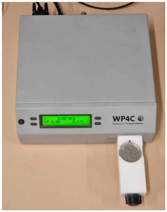
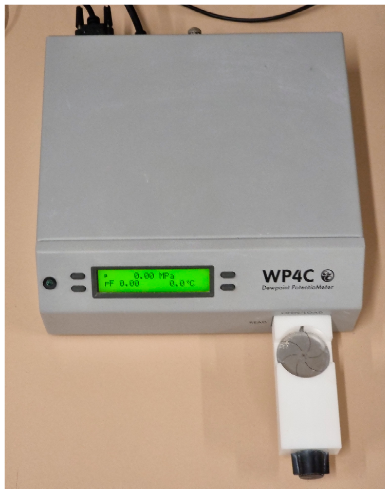
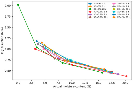
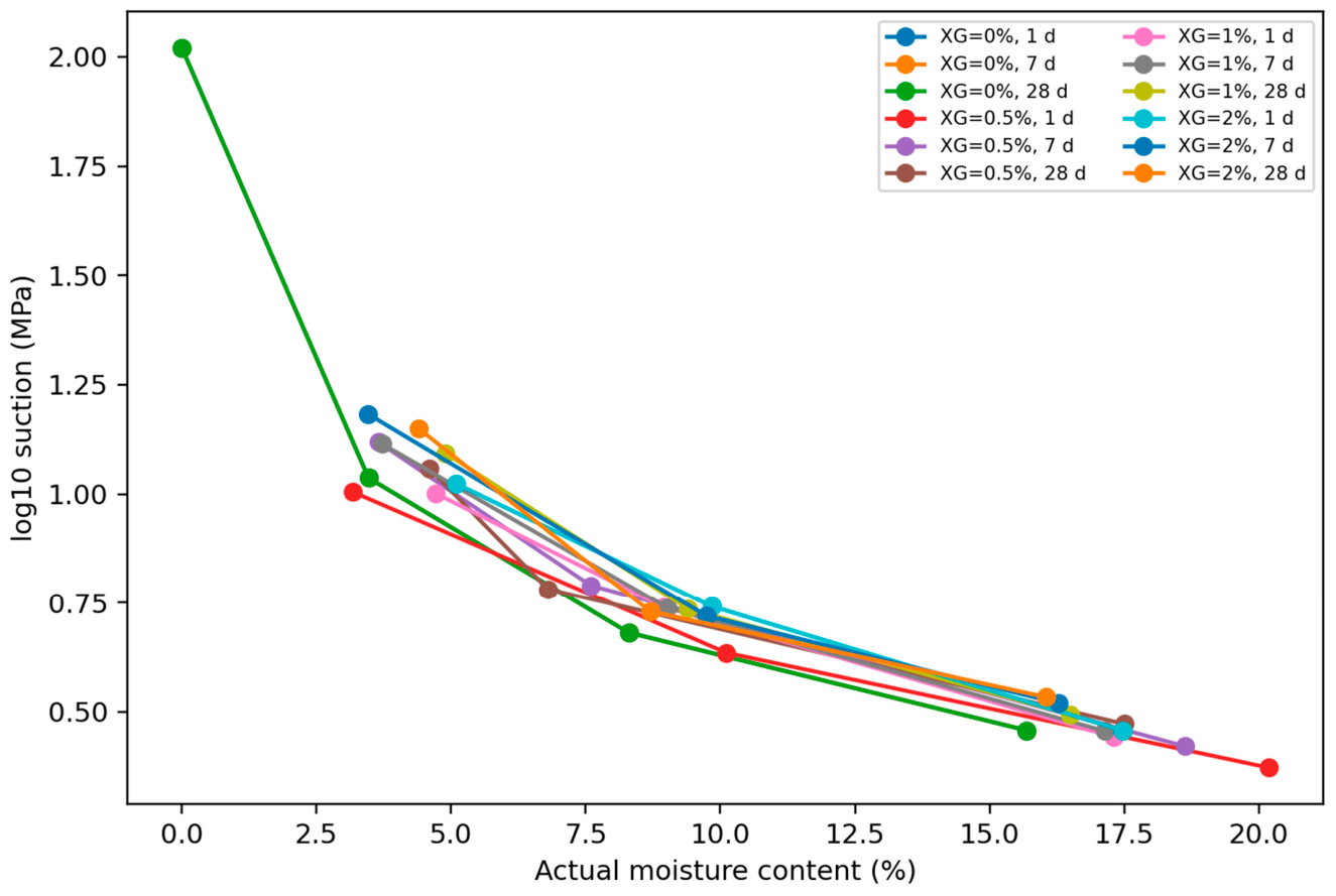
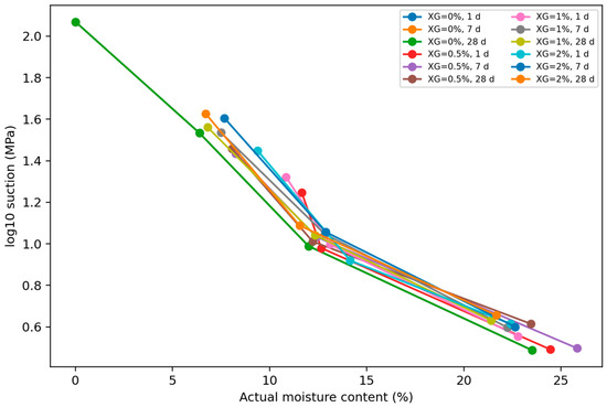
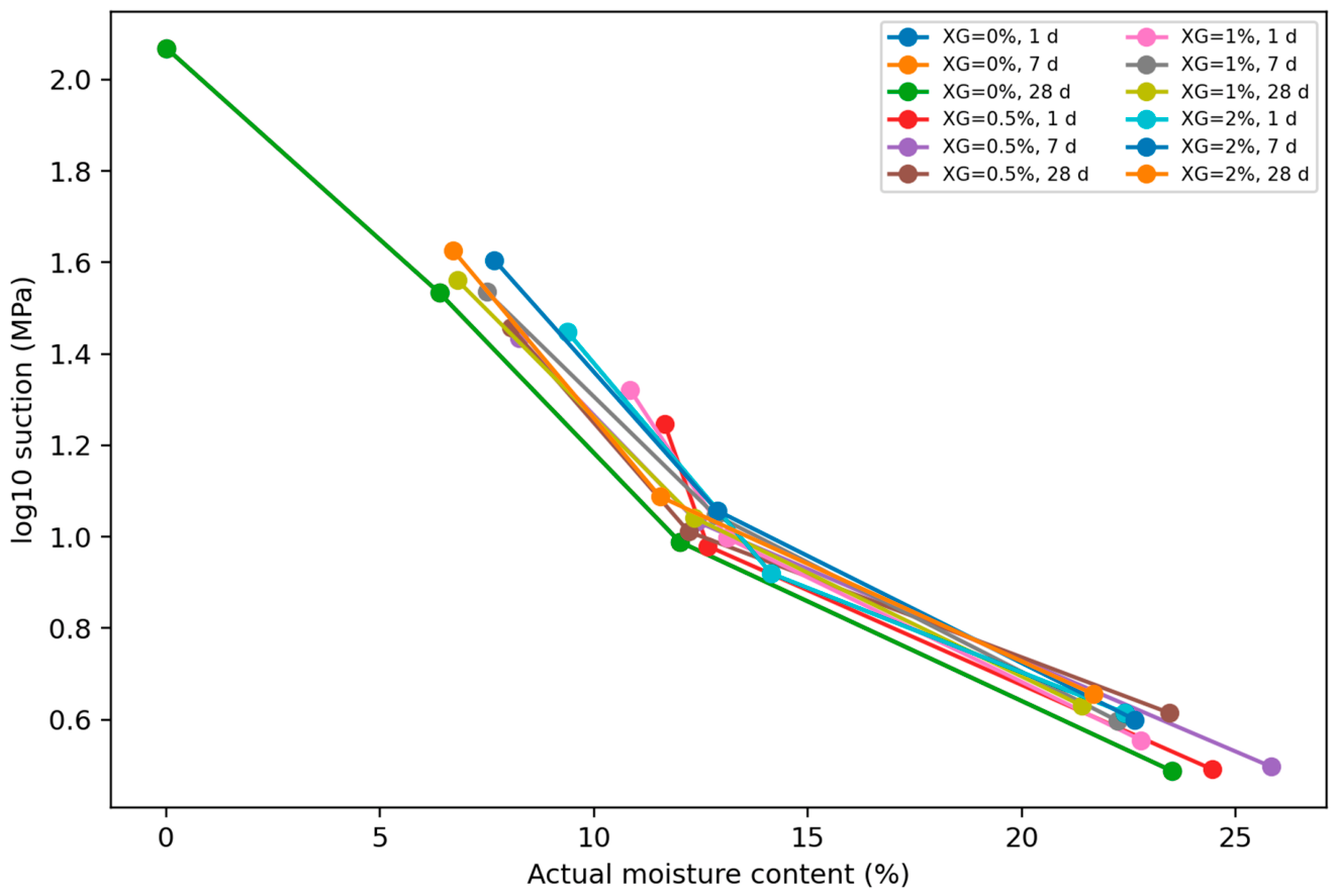
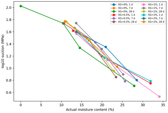
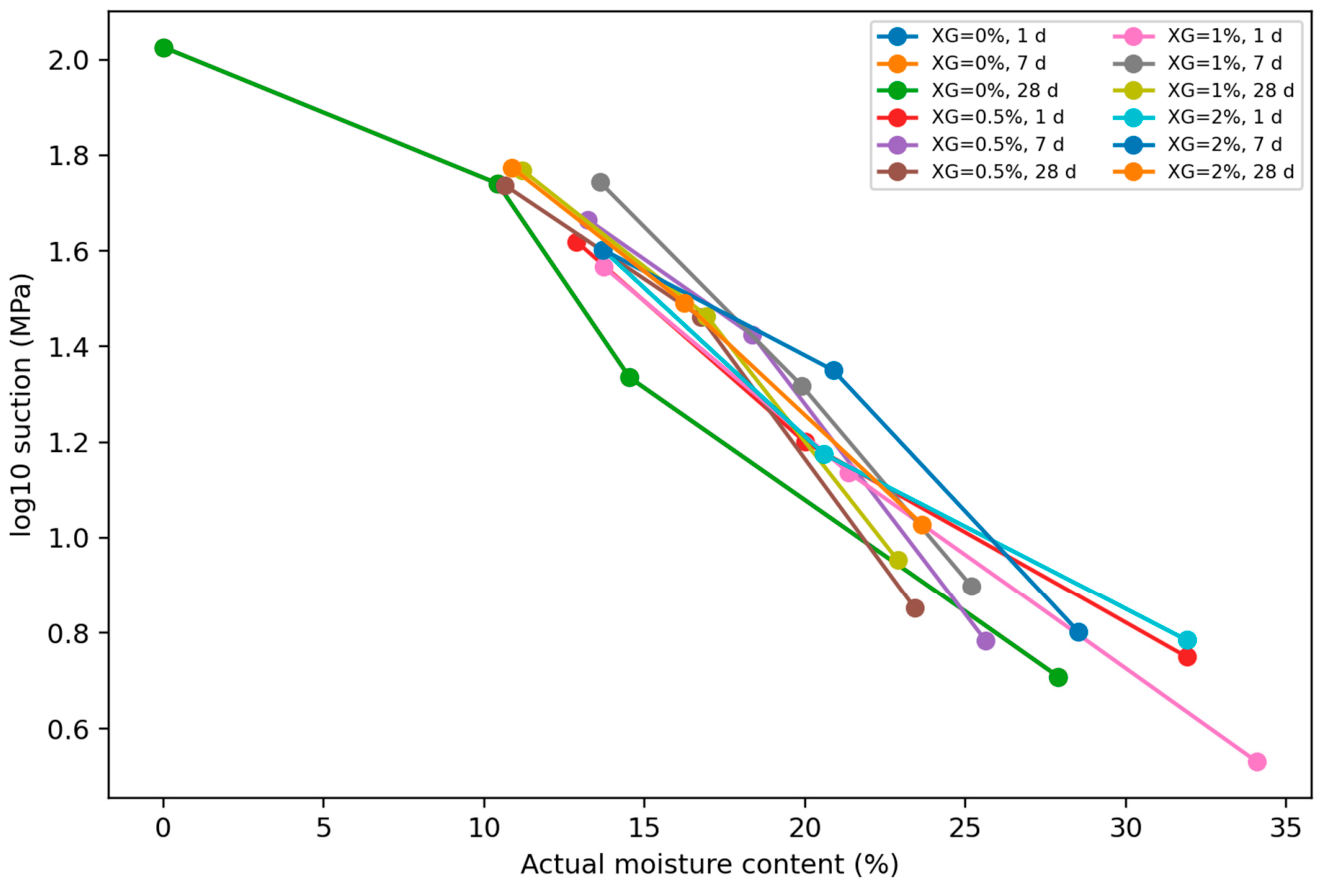
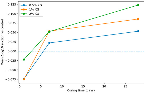
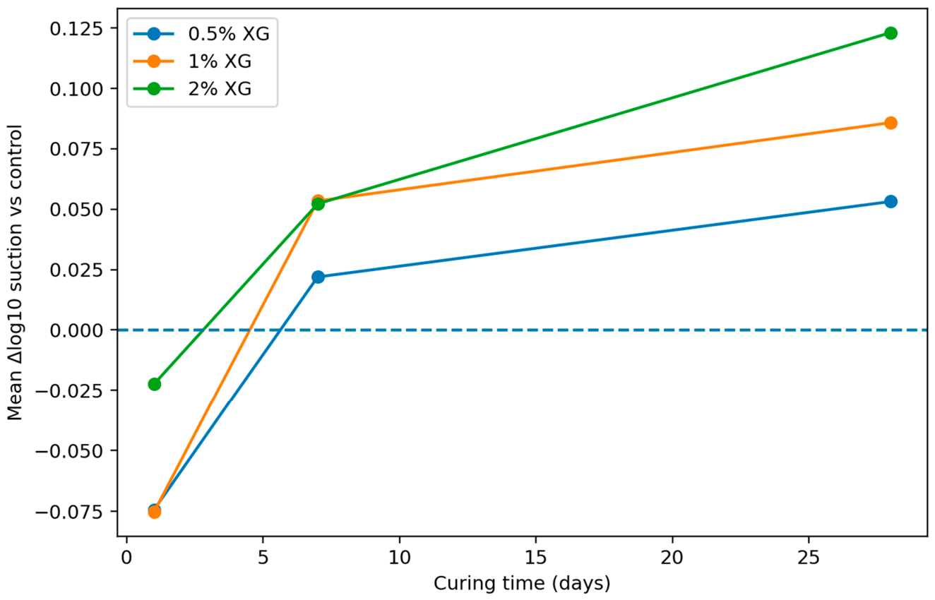
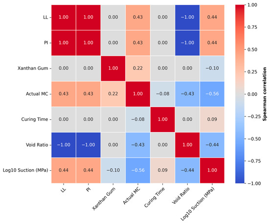
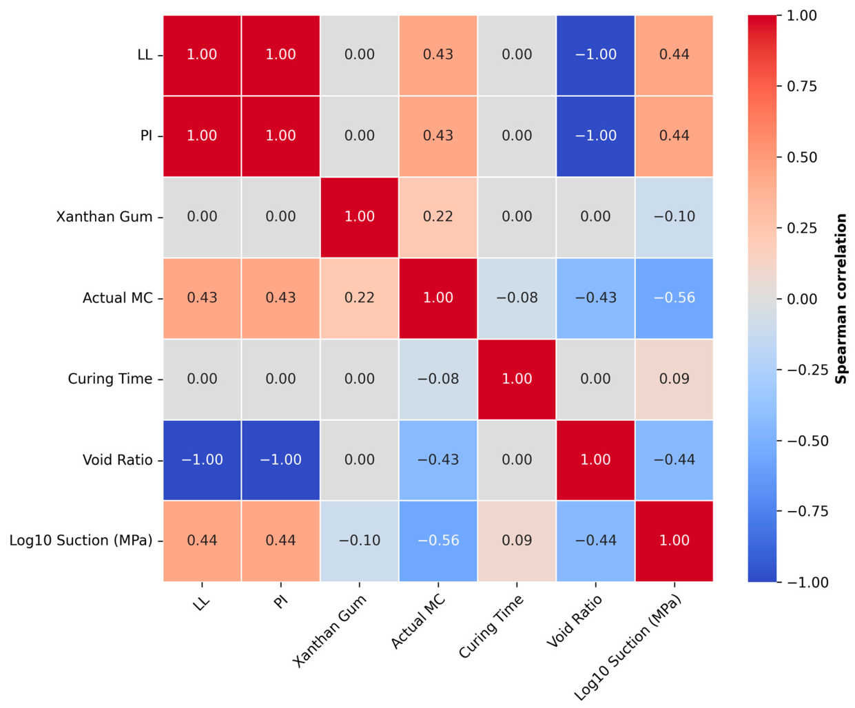
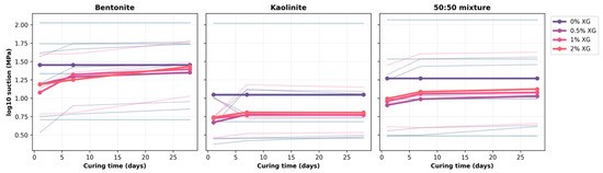
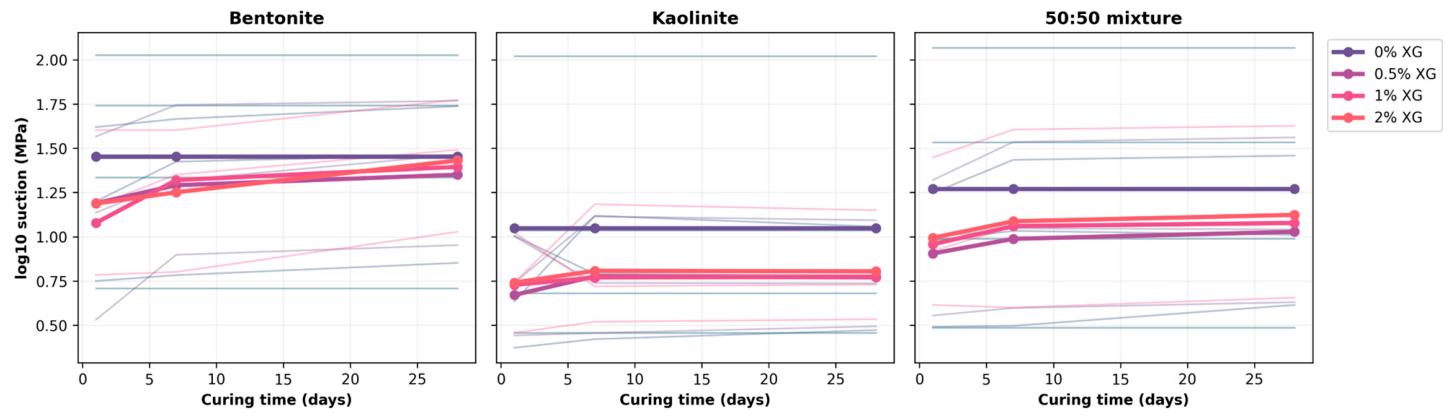
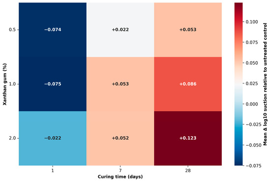
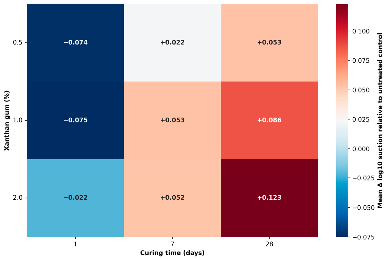
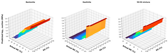
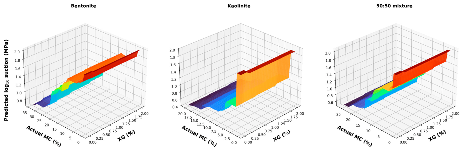
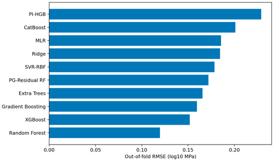
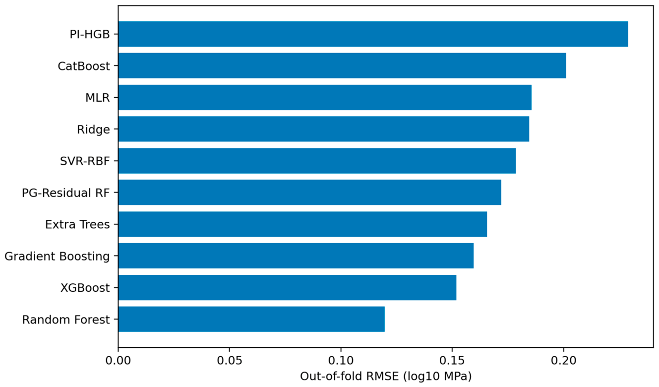
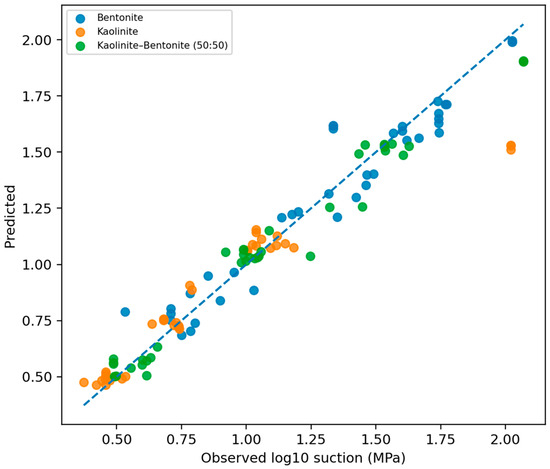
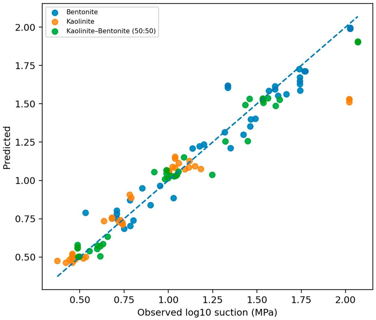
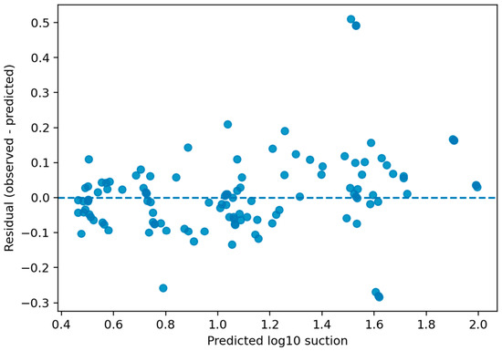
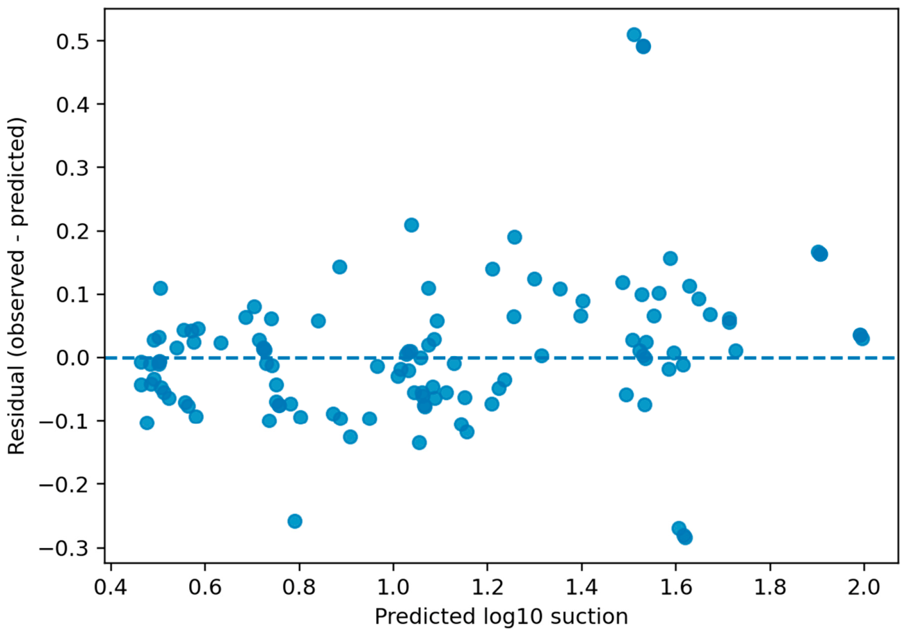
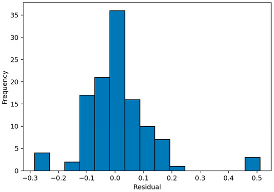
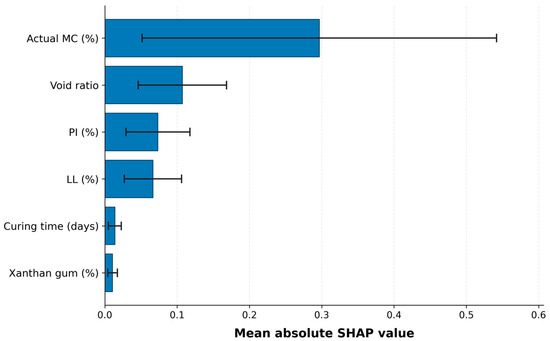
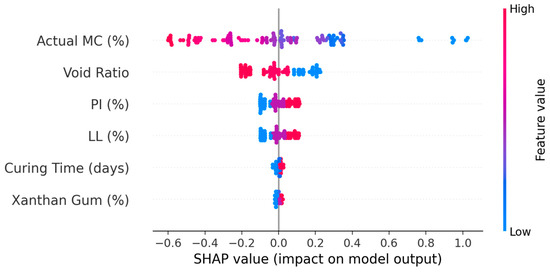
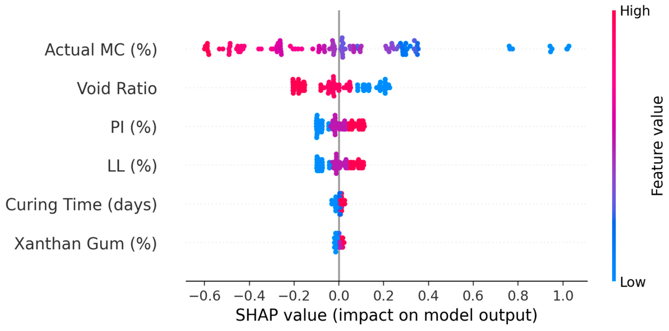
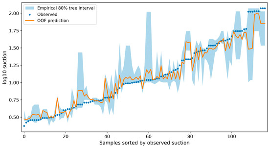
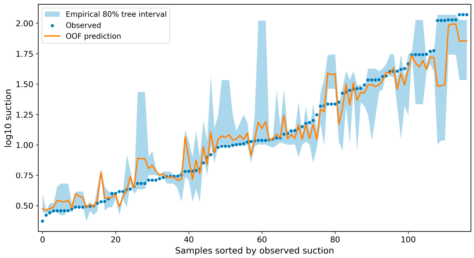
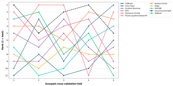
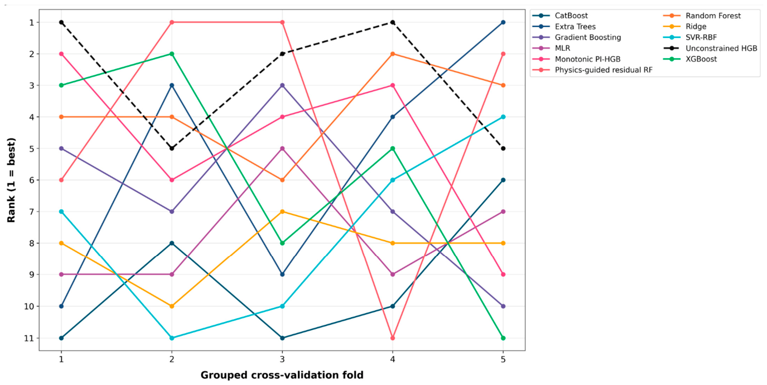
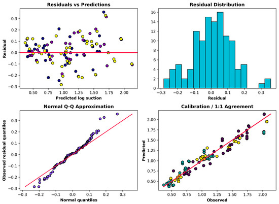
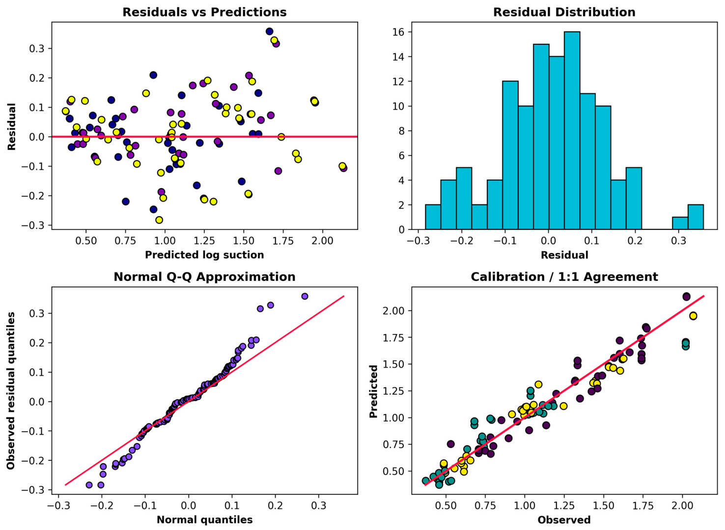
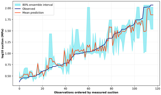
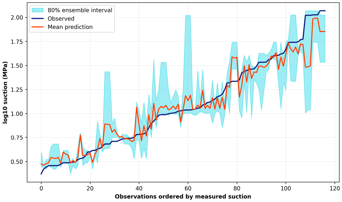
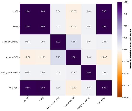
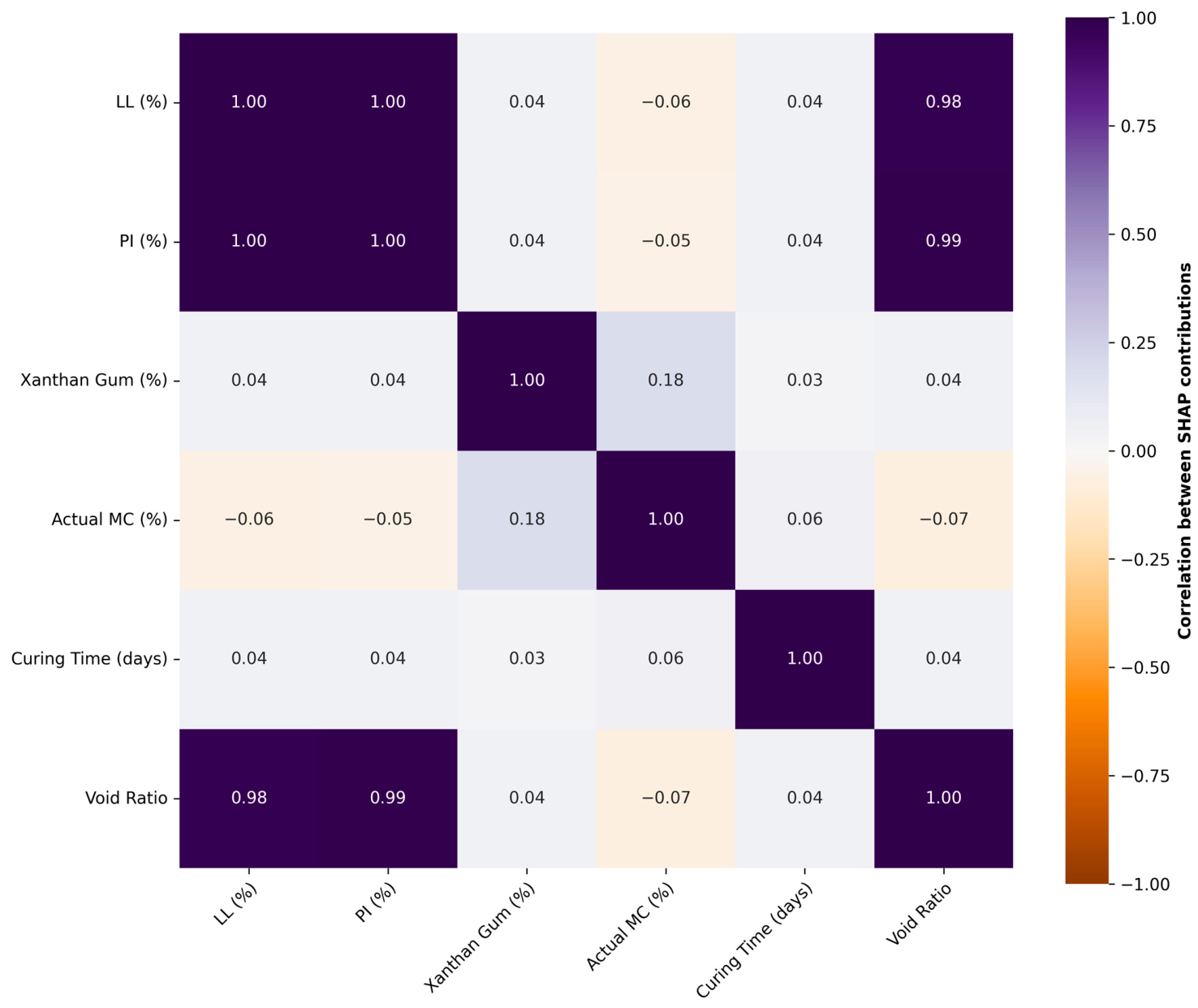
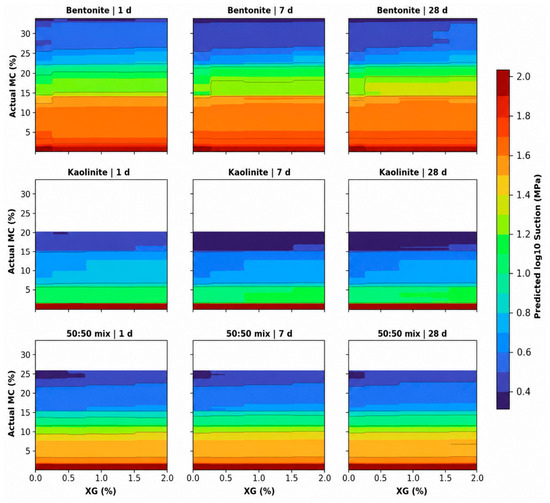
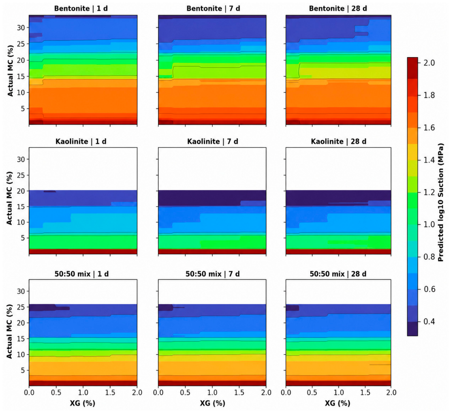

Disclaimer/Publisher’s Note: The statements, opinions and data contained in all publications are solely those of the individual author(s) and contributor(s) and not of MDPI and/or the editor(s). MDPI and/or the editor(s) disclaim responsibility for any injury to people or property resulting from any ideas, methods, instructions or products referred to in the content. |
© 2026 by the authors. Licensee MDPI, Basel, Switzerland. This article is an open access article distributed under the terms and conditions of the Creative Commons Attribution (CC BY) license.