DOA Estimation for Underwater Coprime Arrays with Sensor Failure Based on Segmented Array Validation and Multipath Matching Pursuit

Abstract

Coprime arrays enable enhanced degrees of freedom through the construction of virtual array equivalent signals. However, the presence of large “holes” leads to discontinuous co-arrays, which severely hampers direction-of-arrival (DOA) estimation techniques that rely on uniform array structures. This paper explores the practical application of co-array domain signal processing for underwater acoustic coprime arrays. We propose a novel array configuration based on coprime minimum disordered pairs, enabling the formation of continuously connected co-arrays without interpolating. To address the challenge of limited snapshots in underwater environments, DOA estimation can be achieved by utilizing traditional multipath matching pursuit (MMP) algorithms under the proposed continuous co-array implementation scheme. In practical applications, physical array element failures are inevitable, and faulty elements can create holes in the originally continuous co-array. While interpolation techniques can mitigate small gaps, their performance deteriorates significantly in the presence of large holes or uneven data distribution. To overcome these limitations, we introduce a sparse signal recovery (SSR) method using a fragment array data validation technique for sparse DOA estimation with an underwater acoustic coprime array. Based on the designed continuous array expansion scheme, the resulting continuous co-array is used to map the positions of element failures, revealing the gaps in the co-array. A validation model is established for partially continuous sub-arrays within the discontinuous co-array, enabling signal direction estimation based on the fragmented array validation. Both simulation and sea trial results confirm that the proposed approach maximizes the utilization of co-array elements without relying on interpolation or prediction, offering a robust solution for scenarios involving sensor failures.

1. Introduction

Coprime arrays offer enhanced resolution and increased degrees of freedom (DoF) due to their closed-form geometry and reduced sensor mutual coupling. In contrast to Minimum Redundancy Arrays (MRA) [1] and Minimum Hole Arrays (MHA) [2], which rely on optimization procedures or precomputed look-up tables, coprime array configurations are defined by a clear and unambiguous analytical expression. The enhanced maximum inter-element spacing constraint-based sparse array (EMISC) array can achieve a performance balance between uniform DOF and mutual coupling [3], but it offers limited additional advantages in underwater acoustic array scenarios. As a result, coprime arrays have attracted considerable interest across a wide range of applications, including radar, speech processing, communications, and underwater acoustics.

Current coprime array signal processing techniques primarily operate within the physical array and co-array domains. In the physical domain, research has focused on analyzing the beamwidth and array gain (AG) characteristics of coprime array beamforming [4]. A key finding is that a coprime linear array with $M+N-1$ elements can achieve an array gain equivalent to that of a full uniform linear array (ULA) with $MN$ elements, resulting in a logarithmic gain of $10log\left(MN\right)$. Classical physical-domain processing methods for coprime arrays include the Product and Min processors. The Product processor calculates the conventional beamformer output for each subarray and then multiplies the output of one subarray by the complex conjugate of the other’s output [5,6,7,8]. In contrast, the Min processor selects the minimum power between the two subarrays’ scanned responses at each bearing [9,10,11]. However, both methods are limited by high grating lobes and elevated sidelobe levels. These limitations have driven extensive research into extensions and modifications of the coprime array structure. For instance, studies have examined the positioning of peak sidelobes in extended coprime sensor arrays [12,13], establishing conditions on the extension factor to ensure sidelobe levels remain below those of a full ULA. Other works have designed array factors to produce beam responses with amplitudes opposite to those of one coprime subarray [14], effectively reducing peak sidelobes at the cost of broader mainlobe widths. Additionally, a novel direction-of-arrival (DOA) estimation method has been proposed using a decomposed coprime linear array (CLA). This method formulates a joint optimization problem for covariance matrix reconstruction, specifically targeting the interference-plus-noise covariance matrix, and subsequently computes the optimal weight vector for a Minimum Variance Distortionless Response (MVDR) beamformer [15,16].

Signal processing in the co-array domain has been extensively studied, particularly in radar applications. Most established methods rely on reconstructing the covariance matrix of the received signal. For example, one approach utilizes a sliding window scheme for covariance matrix reconstruction to facilitate source localization, followed by recalculating the signal power for each source based on the estimated directions-of-arrival (DOAs) [17]. Another method exploits the rotational invariance property of an interpolated coprime array covariance matrix to estimate DOAs without the need for exhaustive spectral searches [18]. These techniques primarily aim to improve the effective DoF and resolution of the array system. Beyond localization, a variety of advanced techniques have been proposed to address practical radar requirements. These include tensor-based processing methods [19,20], adaptive moving coprime array configurations [21], and the application of the annihilating filter concept [22]. A persistent challenge in coprime arrays arises from the discontinuities in the derived co-array-positions without virtual elements, commonly referred to as “holes.” Traditional subspace-based DOA estimation algorithms typically utilize only the longest contiguous segment of the co-array, effectively ignoring information from non-contiguous virtual elements [23]. To fully exploit the entire co-array aperture, numerous interpolation-based DOA estimation methods have been developed. These include techniques based on nuclear norm minimization (NNM) [24,25], gridless methods employing low-rank Toeplitz covariance matrix reconstruction [26], and algorithms that integrate atomic norm minimization (ANM) with Toeplitz matrix reconstruction [27]. While these methods offer improved estimation performance by leveraging the full coarray structure, their high computational complexity significantly limits their practicality in real-world engineeringapplications. These methods offer improved estimation performance by leveraging the full co-array structure. The NNM algorithm is well-suited for scenarios with sufficient signal snapshots, but its performance degrades significantly when the number of snapshots is limited. Similarly, the reconstruction accuracy of the ANM method is adversely affected under low signal-to-noise ratio (SNR) conditions. These limitations restrict the practical applicability of both algorithms in underwater environments. Furthermore, certain studies have pursued the design of hole-free arrays from an array optimization perspective. By configuring multiple subarrays and optimizing their assembly, these approaches achieve hole filling in the virtual array [28]. Through multilayer replication of subarrays, a virtual array containing holes at multiple levels is generated. The holes are categorized into the original layer-gaps inherent between the original subarrays-and the replication layer-holes introduced by the replicated subarrays. These cross-layer holes are subsequently filled by strategically adding supplementary subarrays [29]. Additionally, there are improved methods based on existing coprime array structures that reduce virtual array holes through sensor repositioning, optimization of subarray spacing, or completion of missing inter-layer subarrays [30,31]. Novel coprime arrays are designed by adding sparse subarrays and widening the spacing between subarrays to achieve a hole-free virtual array [32]. Such array configurations successfully balance hole-free difference coarray (DCA) performance with low mutual coupling, while also maximizing the uniform degrees of freedom (uDOFs) through optimal parameter design. The resulting high degree of freedom is particularly valuable in target detection applications such as radar systems. Among other methods based on interpolation and optimization, the interpolation-based method mainly includes array interpolation methods used in the subspace DOA [33,34,35]. These methods rely on array interpolation to fill spatial holes for DOA estimation, making them suitable only for limited scenarios. They lack robustness when facing practical constraints such as large-scale holes, array element failures, and underwater scenarios with limited snapshots. Algorithms Alternating Projection-based Maximum Likelihood Estimation (AP-based ML) [36,37], Root Sparse Bayesian Learning (Root SBL) [38] and Variational Bayesian Inference for Real-valued Sparse Bayesian Learning (VBI) [39] achieve DOA parameter estimation based on optimization methods, but their performance is significantly affected by variations in the number of signal snapshots and SNRs.

In recent underwater acoustic array signal processing, research on coprime array signal processing within underwater acoustic environments remains relatively limited [40]. Investigations into underwater coprime array design have primarily focused on analyzing the performance of Product and Min processors [41,42,43]. Furthermore, an extended coprime hydrophone array configuration was proposed to enhance beamforming resolution and robustness [44]. The inherent complexity of the marine environment poses a significant challenge: it often precludes long-term stationarity in signals received by underwater sonar arrays. This necessitates the development of high-resolution target detection methods capable of operating effectively with limited snapshot data [45,46,47,48,49]. Coprime arrays, as a form of sparse array, offer the significant advantage of substantially expanding the array aperture with a limited number of elements. This inherent sparsity facilitates the construction of a co-array domain, which enables effective signal processing even with limited snapshot availability.

However, in practical underwater deployments, sensor failures pose a critical challenge: they introduce additional, potentially large, holes within the derived co-array. This degradation of the co-array structure renders conventional DOA estimation methods designed for uniform arrays inapplicable. Critically, existing co-array interpolation techniques often fail to adequately compensate for these excessively large holes induced by failures, ultimately degrading the effectiveness of co-array data processing in practical scenarios.

Building upon the aforementioned challenges, this paper proposes a DOA estimation method based on fragment array data validation. We investigate the necessary conditions for achieving a consistent and contiguous co-array, a key concept in coprime array signal processing [50]. A novel array configuration utilizing coprime minimum disordered pairs is proposed, which facilitates the formation of a continuously connected co-array without the need for interpolation. In particular, we address the challenge of sparse signal recovery (SSR) within this context. Array element failures can disrupt the continuity of the array, posing significant obstacles to accurate estimation. This work systematically explores scenarios that lead to such discontinuities, offers a detailed analysis of element failures, and introduces a robust DOA estimation method designed to perform effectively even with discontinuous arrays. The method presented in this paper enables high-resolution underwater DOA estimation and robust signal processing, even in the presence of array element damage, which is an important advancement for engineering applications. The effectiveness of the proposed approach is demonstrated through both simulation and sea trial data.

The remainder of this paper is organized as follows. Section 2 introduces the mathematical signal model for the coprime array and derives the co-array structure resulting from the proposed expansion using the coprime minimum disordered pair. In Section 3, we present the DOA estimation algorithm tailored for co-arrays with large-scale discontinuities, and detail the FADV approach for handling such fragmentation. Section 4 provides simulation-based validation, while Section 5 presents results from sea trial data processing. Finally, conclusions are drawn in Section 6.

2. Signal Model

A typical coprime array comprises two uniform sparse subarrays. One subarray contains M elements with an inter-element spacing of $Nd$, while the other contains N elements with an inter-element spacing of $Md$ [7,51]. $d=\lambda /2$ denotes the unit sensor spacing, where $\lambda$ is the wavelength of the narrowband signal incident on the array. Here, M and N are coprime integers. The array configuration is expressed as

$$\mathbb{S}=\{Mnd,0\le n\le N-1\}\cup \{Nmd,0\le m\le M-1\}.$$

(1)

Considering that L far-field, uncorrelated and narrow-band signals impinged on the coprime array from directions ${\theta }_l$, $l=1,2,\dots ,L$. The signals received by the coprime array at time t can be modeled as

$$\mathit{x}\left(t\right)=\mathit{As}\left(t\right)+\mathit{n}\left(t\right)$$

(2)

where $\mathit{s}\left(t\right)={[s_1\left(t\right),s_2\left(t\right),\dots ,s_L\left(t\right)]}^T$ represents the signal waveform vector, and $\mathit{n}\left(t\right)\sim \mathcal{CN}(0,{\sigma }_n^2\mathit{I})$ denotes the independent and identically distributed Gaussian noise component with variance ${\sigma }_n^2$, where ${\sigma }_n^2$ is the noise power and $\mathit{I}$ stands for the identity matrix. The l-th source signal’s steering vector is represented by the l-th column of $\mathit{A}$, which can be formulated as

$$\mathit{a}\left({\theta }_l\right)=[1,exp(-j{\displaystyle \frac{2\pi }{\lambda }}{d}_{2}sin\left({\theta }_l\right)),\dots ,exp(-j{\displaystyle \frac{2\pi }{\lambda }}{d}_{M+N-1}sin\left({\theta }_l\right))]$$

(3)

where $d_i\in \mathbb{S}$, $i=1,2,\dots ,M+N-1$ and $j=\sqrt{-1}$.

2.1. Signal Model for the Co-Array from the Coprime Array

The co-array signals can be derived by vectorizing the covariance matrix. In this context, the signal covariance matrix is expressed as

$$\mathit{R}=E\left[\mathit{x}\left(t\right){\mathit{x}}^H\left(t\right)\right]=\sum _{l=1}^L{p}_l\mathit{a}\left({\theta }_l\right){\mathit{a}}^H\left({\theta }_l\right)+{\sigma }_n^2\mathit{I}$$

(4)

where $p_l$ represents the power of the l-th source signal. In practical applications, $\mathit{R}$ can be approximated as

$$\widehat{\mathit{R}}={\displaystyle \frac{1}{T}}\sum _{t=1}^T\mathit{x}\left(t\right){\mathit{x}}^H\left(t\right).$$

(5)

When the covariance matrix is vectorized, the co-array signals can be obtained as

$$\mathit{v}=vec\left(\mathit{R}\right)={\mathit{A}}_v\mathit{p}+{\sigma }_n^2\mathit{u}$$

(6)

where ${\mathit{A}}_v=[{\mathit{a}}^{*}\left({\theta }_1\right)\otimes \mathit{a}\left({\theta }_1\right),{\mathit{a}}^{*}\left({\theta }_2\right)\otimes \mathit{a}\left({\theta }_2\right),\dots ,{\mathit{a}}^{*}\left({\theta }_L\right)\otimes \mathit{a}\left({\theta }_L\right)]$, $\mathit{u}=\mathrm{vec}\left(\mathit{I}\right)$, and $\mathit{p}={[p_1,p_2,\dots ,p_L]}^T$. ${\mathit{A}}_v$ can be constructed based on $\mathbb{D}$, which is the difference set of a coprime array and can be expressed as

$$\mathbb{D}=\left\{\mathsf{\ell }\left|\mathsf{\ell }=\pm (Mn-Nm),0\le n\le N-1,0\le m\le M-1\right.\right\}.$$

(7)

2.2. A Consistent Array Extension Scheme for Generating Hole-Free Co-Arrays

Co-arrays with a greater number of continuous elements can be obtained by expanding the coprime array from the physical array domain [23]. This paper will investigate the continuity of the difference co-array generated by coprime subarrays under the influence of the same array expansion factor.

Assume that the coprime array consists of two linear subarrays $A_1$ and $A_2$ with overlapping first elements, satisfying $gcd(M,N)=1$, where M and N represent the number of elements in subarrays $A_1$ and $A_2$, respectively. Subarray $A_1$ has an element spacing of $Nd$, and its position set is defined as $P_1=\left\{n_{1}Nd\mid n_1=0,1,\dots ,M-1\right\}$. Subarray $A_2$ has an element spacing of $Md$, and its position set is defined as $P_2=\left\{n_{2}Md\mid n_2=0,1,\dots ,N-1\right\}$.

When the subarray expansion factor $\alpha \in {\mathbb{N}}^{+}$, the expanded subarray $A_1^{\alpha }$ consists of $\alpha M$ elements, with its position set defined as $P_1^{\alpha }=\left\{k_{1}Nd\mid k_1=0,1,\dots ,\alpha M-1\right\}$; the expanded subarray $A_2^{\alpha }$ consists of $\alpha N$ elements, with its position set given by $P_2^{\alpha }=\left\{k_{2}Md\mid k_2=0,1,\dots ,\alpha N-1\right\}$; and the physical position set of the overall expanded array is expressed as $P^{\alpha }=P_1^{\alpha }\cup P_2^{\alpha }$.

Definition of a hole-Free co-array:

The co-array $P_{co}^{\alpha }$ generated by the set of position differences between physical array elements, satisfies

$$P_{co}^{\alpha }=\left\{p_i-p_j|p_i,p_j\in P^{\alpha }\right\}.$$

(8)

For any expansion factor $\alpha$, there exists an integer $L_{\alpha }\in {\mathbb{N}}^{+}$ ensuring that

$$\left\{-L_{\alpha }d,-(L_{\alpha }-1)d,\dots ,0,(L_{\alpha }-1)d,L_{\alpha }d\right\}\in P_{co}^{\alpha },$$

(9)

which implies that all integer multiples of the unit spacing d within the interval $\left[-\left(L_{\alpha }d\right),L_{\alpha }d\right]$ are covered. A co-array fulfilling this condition is said to be hole-free.

The co-array consists of three types of position differences.

(1)

The differences within subarray $A_1^{\alpha }$

$$△P_1^{\alpha }=\left\{N(k_1^{\prime }-k_1^{″})d|k_1^{\prime },k_1^{″}\in \left[0,\alpha M-1\right]\right\},$$

(10)

covering all integer multiples of N;

(2)

The differences within subarray $A_2^{\alpha }$

$$△P_2^{\alpha }=\left\{M(k_2^{\prime }-k_2^{″})d|k_2^{\prime },k_2^{″}\in \left[0,\alpha N-1\right]\right\},$$

(11)

covering all integer multiples of M;

(3)

The differences cross two subarrays

$$△P_{12}^{\alpha }=\left\{M{k}_{2}d-N{k}_{1}d|k_1\in \left[0,\alpha M-1\right],k_2\in \left[0,\alpha N-1\right]\right\},$$

(12)

corresponding to the linear combination $(M{k}_2-N{k}_1)d$.

For a co-array without holes, the necessary and sufficient condition is that for any integer t, one of the following conditions must be satisfied: t is a multiple of M (covered by $△P_2^{\alpha }$); t is a multiple of N (covered by $△P_1^{\alpha }$); t can be expressed as $M{k}_2-N{k}_1$ (or $N{k}_1-M{k}_2$), where $k_1\in \left[0,\alpha M-1\right]$, $k_2\in \left[0,\alpha N-1\right]$ (covered by $△P_{12}^{\alpha }$).

Given that $gcd(M,N)=1$, by Bezout’s theorem fulton2008algebraic, there exist integers $x_0$ and $y_0$ such that $M{x}_0+N{y}_0=1$. This indicates that for any integer t, taking $x=t{x}_0$ and $y=t{y}_0$ yields $Mx+Ny=t$.

Since the array element indices are nonnegative, $k_1$ and $k_2$ must satisfy the expanded index range constraints $k_1\le \alpha M-1$ and $k_2\le \alpha N-1$. The problem now reduces to determining whether, for any $\alpha \in {\mathbb{N}}^{+}$ and any integer t, there exist nonnegative integers $k_1$ and $k_2$ satisfying $M{k}_2-N{k}_1=t$ and $k_1\le \alpha M-1$, $k_2\le \alpha N-1$.

In the linear combination $M{k}_2-N{k}_1$ (or $N{k}_1-M{k}_2$), the smaller the values of the pair M and N, the smaller the required $k_1$ and $k_2$ for generating any integer, making it easier to satisfy the expanded index range constraints.

The minimum unordered pair can be represented as

$${\mathbb{U}}_{CMDP}=\{(2,3),(3,2)\}.$$

(13)

Its peculiarity lies in the fact that for any expansion factor $\alpha$, the range of physical element indices after scaling is

$$\left\{\begin{array}{c}{k}_1\in \left[0,2\alpha -1\right]\\ k_2\in \left[0,3\alpha -1\right]\end{array}\right..$$

(14)

The maximum aperture of the co-array is determined by the maximum position difference of physical elements, which can be expressed as

$$max\left(P^{\alpha }\right)-min\left(P^{\alpha }\right)=max(3(2\alpha -1),2(3\alpha -1))d=(6\alpha -2)d.$$

(15)

The positions of virtual elements cover the interval $[-(6\alpha -2)d,(6\alpha -2\left)d\right]$. Within this interval, all even positions are covered by $△P_2^{\alpha }$, all odd positions are covered by $△P_{12}^{\alpha }$, and all integer multiples of 3 are covered by $△P_1^{\alpha }$. Therefore, there are no holes in the interval, and this conclusion holds for any $\alpha$. Similarly, the pair $(3,2)$ also satisfies the condition that the co-array is free of holes for any expansion factor $\alpha$.

When $(M,N)\ne {\mathbb{U}}_{CMDP}$, the increased coefficients lead to larger values for the non-negative integer pair $(k_1,k_2)$ required to generate an arbitrary integer. For small values of $\alpha$, the upper bound of the discrete index range in the extended sub-arrays is low, and the non-negative integer pair $(k_1,k_2)$ needed to produce the integer exceeds the constraint boundaries of the range. Even when $\alpha$ increases, because the least common multiple of M and N is relatively large, certain integers still cannot be generated via the linear combination $M{k}_2-N{k}_1$. These uncovered integer positions are multiples of neither M nor N, ultimately resulting in holes in the virtual array. As shown in Table 1, the table presents co-array null positions under different coprime number pairs and different array expansion factors. The array element positions in the table are normalized, with the unit element spacing d omitted.

Table 1. Comparison Table of Co-array Null Positions Under Different Coprime Pairs and Expansion Factors.

(M, N)	$\mathit{\alpha }$	Coverage Range	Null Positions
${\mathbb{U}}_{CMDP}$	2	[−22, 22]	None
${\mathbb{U}}_{CMDP}$	6	[−70, 70]	None
${\mathbb{U}}_{CMDP}$	13	[−154, 154]	None
${\mathbb{U}}_{CMDP}$	19	[−226, 226]	None
(3, 5)	2	[−27, 27]	$\pm 23,\pm 26$
(3, 5)	6	[−87, 87]	$\pm 83,\pm 86$
(3, 5)	13	[−192, 192]	$\pm 191,\pm 188$
(5, 7)	2	[−65, 65]	$\pm 47,\pm 52,\pm 54,\pm 57,\pm 59,\pm 61,\pm 62,\pm 64$
(5, 7)	6	[−205, 205]	$\pm 187,\pm 192,\pm 194,\pm 197,\pm 199,\pm 201,\pm 202,\pm 204$

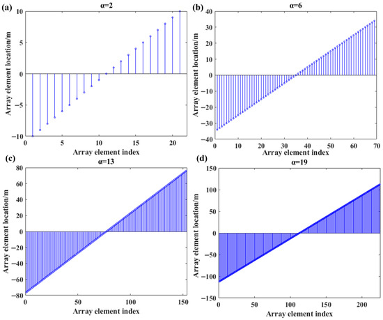
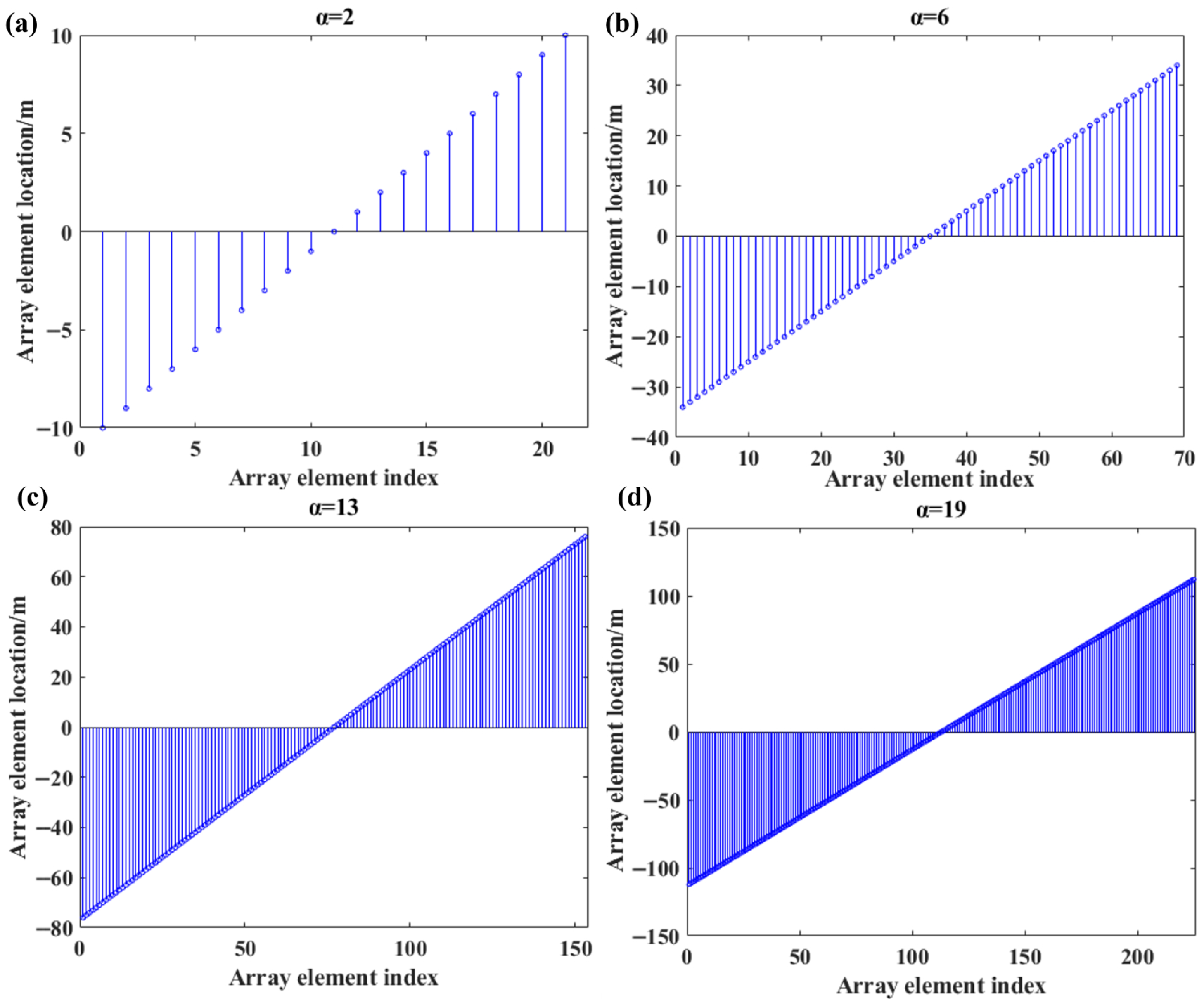
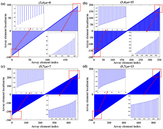
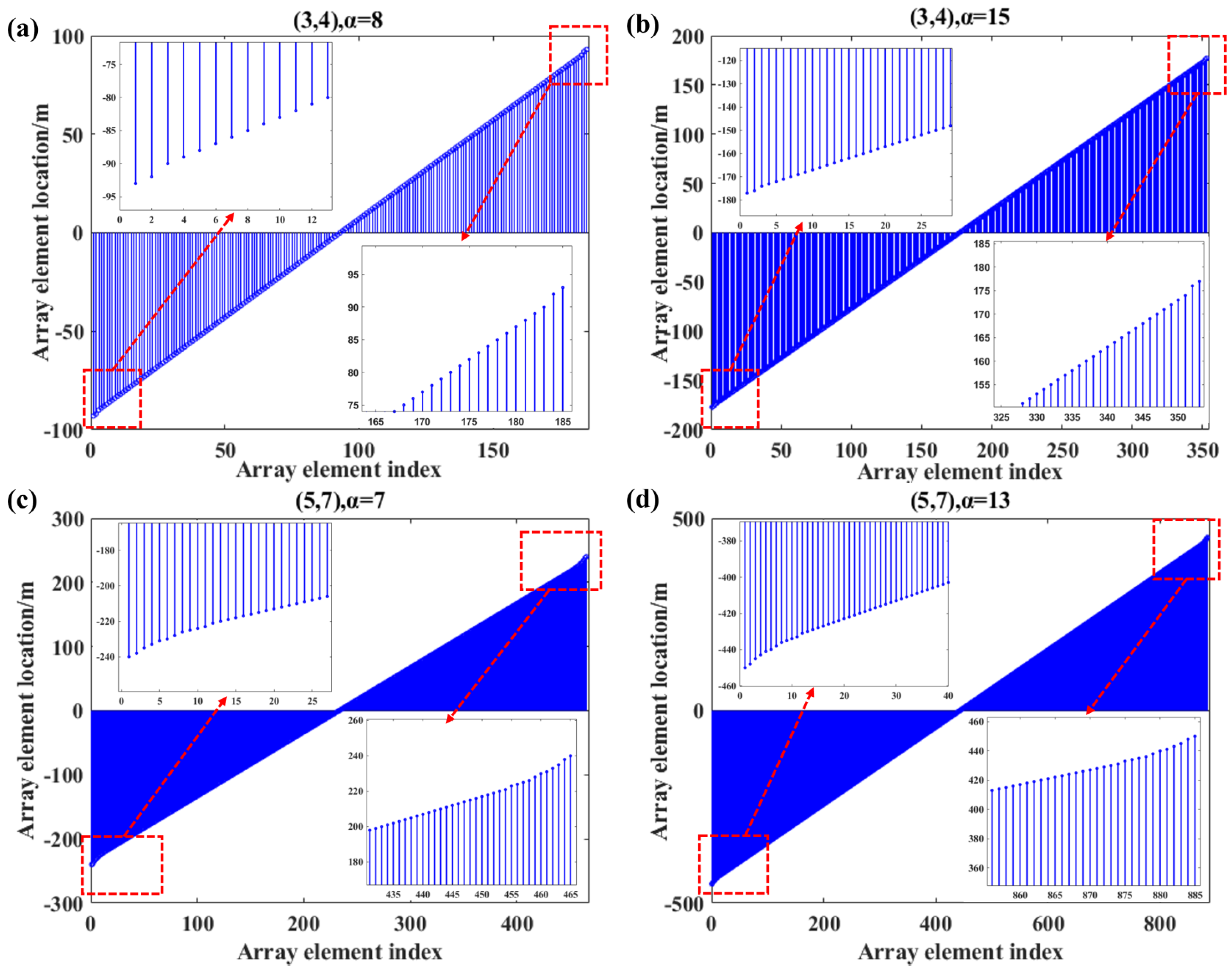
Figure 1 and Figure 2 illustrate co-arrays constructed with and without the coprime minimum disordered pair, respectively. As shown in Figure 1, co-arrays based on the coprime minimum disordered pair consistently yield continuous arrays without any “holes”. However, other coprime array pairs fail to ensure the continuity of the virtual array expanded under any expansion factor. By minimizing the element spacing of the coprime expanded subarrays, CMDP enables the mapping of these subarrays to the virtual domain, covering all element spacings of the complete virtual array. Furthermore, ref. [7] illustrates that virtual array generation is a process involving covariance vectorization and the search for element spacing differences (as well as virtual array element positions). This advantage eliminates the need for additional processing to fill array “holes”, such as virtual interpolation or array element prediction, allowing the complete co-array to be fully utilized. In contrast, when the extended array is not based on the coprime minimum disordered pair, the resulting co-array may be inhomogeneous and contain holes. For example, when $M=3$, $N=4$, and the array expansion factor is a random integer, as shown in Figure 2a,b; and when $M=5$, $N=7$, and the array expansion factor is a random integer, as shown in Figure 2c. It is evident from Figure 2 that all the generated co-arrays are discontinuous.

Figure 1. The co-array elements arrangement based on the coprime minimum disordered pair and random array extension factors $\alpha$. (a) $\alpha =29$. (b) $\alpha =6$. (c) $\alpha =13$. (d) $\alpha =19$.

Figure 2. Disconnected co-array elements arrangement based on non-coprime minimum disordered pair and random array extension factors $\alpha$. (a) $(M,N)=(3,4)$ with $\alpha =8$. (b) $(M,N)=(3,4)$ with $\alpha =15$. (c) $(M,N)=(5,7)$ with $\alpha =7$. (d) $(M,N)=(5,7)$ with $\alpha =13$.

The co-array discontinuity becomes more pronounced when the two sub-arrays have different expansion factors. Extracting only the continuous portion of the co-array for signal processing results in significant waste of both the computed data and the additional resources represented by the co-array elements. In some hole-free coarray configurations, such as the Hole-Free Coprime Array (HFCA) [28], the approach differs from the extended array based on the minimal coprime pair proposed in this paper. Instead of expanding the original coprime array, HFCA starts from an unextended prototype and establishes multiple subarrays. The positional relationships among these subarrays generate a union of virtual elements that collectively form a complete virtual array. While this design can enhance the array’s uniform degrees of freedom (uDOFs), it imposes constraints on the number of physical sensors, often resulting in a large array aperture. This makes it difficult to implement in systems with a limited number of array elements. Similarly, the Multi-Layer Filled Coprime Array (MLFCA) [29] employs a multi-layer hole-filling strategy to achieve a hole-free coarray. Due to its hierarchical filling mechanism, this method also requires a relatively large number of physical sensors, making it unsuitable for arrays with few elements. Moreover, the implementation process involves removing specific sensors and adjusting subarray positions, which significantly increases the complexity of sensor calibration in practical deployments.

3. DOA Estimation for Co-Arrays with Large-Scale Holes

3.1. Hole Discrimination and Reconstruction of Co-Arrays

From Equation (7), it is clear that distinct physical array elements can produce identical virtual array elements. To simplify the discussion, we define a linear array of P sensors, which represents the general form of the array elements described in Equation (1) [52]. The linear array of P sensors

$$\mathit{z}=[n_1{n}_2\dots n_P],$$

(16)

is used to identify the angles at which source signals impinge on the array. The difference co-array, ${\mathbb{D}}_{\mathbf{z}}={\left\{n_i-n_j\right\}}_{i,j=1}^P$, represents the set of all pairwise differences between sensor locations. The co-array weights $w\left(l\right)$ indicate the number of sensor pairs separated by a distance l, i.e.,

$$w\left(l\right)=\left|\{(i,j)\mathrm{where}{n}_i-n_j=l\}\right|$$

(17)

where $\left|·\right|$ denotes the cardinality of the set. When $w\left(l\right)>1$, it indicates that the sensor pair generating the corresponding co-array element can be substituted. If one physical sensor in such a pair fails, other sensor pairs can still be used to generate the same co-array element. However, if the same physical sensor appears in multiple pairs and fails, no alternative pair may exist, resulting in a hole in the co-array. Moreover, when $w\left(l\right)=1$, it implies that only a single pair of physical sensors can generate the corresponding co-array element. In this case, the failure of either sensor in the pair will lead to a hole in the co-array.

3.2. DOA Estimation for Continuous Co-Arrays

Based on Section 2, the covariance vector $\mathit{v}$ of the received signal in the co-array, constructed using the coprime minimum disordered pair, can be expressed as

$$\mathit{v}=\mathbf{\Psi }\mathit{s}$$

(18)

where $\mathit{v}$ is the co-array signal obtained from the co-array generated through covariance vectorization, and its dimension depends on the specific coprime pair used. $\mathit{s}$ is a sparse signal, and the set of indices corresponding to the non-zero elements in $\mathit{s}$ is referred to as the support set. Suppose $\mathit{v}$ has dimension Q, then $\mathit{s}\in {\mathbb{C}}^Q$. The basis matrix $\mathbf{\Psi }$ is a $Q\times Q$ identity matrix. Its specific manifestation is a square matrix where the main diagonal elements are 1 and all other elements are 0 and its corresponding mathematical form is matrix $\mathrm{\Psi }=I_Q$. When Equation (18) holds, the problem of solving for $\mathit{v}$ can be transformed into a sparse signal recovery (SSR) process. In this work, we apply the Multipath Matching Pursuit (MMP) algorithm [53] to co-array processing for coprime arrays. The proposed method eliminates the need to estimate the signal covariance matrix, enabling DOA estimation with only a few snapshots. By employing the measurement matrix $\mathbf{\Phi }\in {\mathbb{C}}^{P\times Q}$, where $P\ll Q$, the sparse signal $\mathit{v}$ is projected onto a lower-dimensional space ${\mathbb{C}}^P$, resulting in the following observed vector for $\mathit{v}$.

$$\mathit{x}=\mathbf{\Phi }\mathit{v}=\mathbf{\Phi }\mathbf{\Psi }\mathit{s}=\mathit{A}\mathit{s}$$

(19)

Since $P\ll Q$, the system of equations in Equation (19) is underdetermined. However, because $\mathit{s}$ is sparse, the number of effective unknowns is much smaller than the dimensionality of the vector. In other words, given that $\mathit{s}$ contains many zero elements, it is possible to recover the signal by solving an optimization problem with significantly fewer unknowns. Here, $\mathit{A}$ denotes the sensing matrix. Assuming that any $2K$ columns of $\mathit{A}$ are linearly independent and that $\mathit{s}$ is K-sparse (i.e., contains at most K non-zero entries), the sparsest solution to the underdetermined system can be obtained by solving the following $l_0$-norm minimization problem:

$$\underset{\mathit{s}}{min}{∥\mathit{s}∥}_{0}subjectto\mathit{A}\mathit{s}=\mathit{x}.$$

(20)

By recovering the sparse vector $\mathit{x}$, the original signal $\mathit{v}$ can be reconstructed. The $l_0$-norm physically represents the number of non-zero elements in a signal x. Solving such problems is fundamentally a combinatorial optimization task, as it requires enumerating all possible K-sparse support sets from a Q-dimensional vector. The complexity of this enumeration is $\left(\begin{array}{c}Q\\ K\end{array}\right)$ and when Q is large, the complexity grows exponentially, making it super-polynomial in time. According to the definition of NP-hardness, this problem cannot be solved optimally in polynomial time, rendering it an NP-hard problem. The MMP algorithm does not directly solve the NP-hard combinatorial optimization problem of the $l_0$-norm. Instead, it relaxes the problem using a greedy heuristic strategy. The MMP algorithm avoids enumerating all possible K-sparse support sets and instead adopts an iterative multi-path exploration of candidate solutions. In each iteration, it simultaneously explores multiple columns that are highly correlated with the current residual $(\mathit{x}-\mathit{A}\mathit{s})$, generating multiple candidate support set paths. Furthermore, based on the premise of the sparsity constraint ${∥\mathit{s}∥}_0=K$, the algorithm relaxes the original $l_0$-norm combinatorial optimization problem into an iterative process of minimizing the residual cost function $\mathit{J}\left(\mathit{s}\right)={∥\mathit{x}-\mathit{A}\mathit{s}∥}_2$. In each step, it selects the support set that minimizes the residual from the candidate paths, gradually updates the sparse vector s, and ultimately obtains an approximate solution that satisfies the sparsity requirement [53].

3.3. DOA Estimation for Co-Array with Large-Scale Holes

A complete and continuous co-array can be achieved using the coprime minimum disordered pair under various array expansion factors. In contrast, co-arrays extended from other coprime pairs not based on the coprime minimum disordered pair are highly likely to exhibit array “holes”. These “holes” fragment the continuous co-array into multiple segments. Accordingly, the positions of the co-array elements can be represented as

$${\mathbb{D}}_{\mathit{c}}=\{\mathsf{\ell }\left|\mathsf{\ell }\in \right.{\mathit{D}}_1\cup {\mathit{D}}_2,\dots ,\cup {\mathit{D}}_i\}$$

(21)

where ${\mathbb{D}}_{\mathit{c}}$ denotes the element positions of the entire co-array, and ${\mathit{D}}_i$ represents the element positions of the i-th continuous array fragment separated by “holes”. Here, i indicates the index of the array fragments.

This section proposes a DOA estimation method based on fragment array data validation for discontinuous co-arrays derived from coprime arrays. In the MMP algorithm applied to the co-array domain of coprime arrays, only a small number of snapshots are required to estimate the DOA of the signals. However, in underwater target detection scenarios, the number of sources is typically unknown, and inaccurate sparsity settings can significantly degrade signal reconstruction performance. To address this, the received signals associated with the discontinuous co-array are divided into two parts, and a compressive sensing approach incorporating fragment array data validation is employed [54]. The multi-snapshot signal model can be derived as Equation (22), based on Equation (6), and the corresponding fragment array data validation term is formulated in Equation (23).

$$\mathit{V}=\mathit{A}\mathit{p}+{\sigma }_n^2\mathit{U}$$

(22)

$${\mathit{V}}_{cv}={\mathit{A}}_{cv}\mathit{p}+{\sigma }_n^2{\mathit{U}}_{cv}$$

(23)

where $\mathit{V}$ serves as the measurement vector, and ${\mathit{V}}_{cv}$ is regarded as the validation vector used in the MMP algorithm for the co-array.

$$\begin{array}{c}\mathit{V}=\{v_{d_1},v_{d_2},\dots ,v_{d_p}\left|d_p\right.\in \mathit{D},\\ \mathrm{where}\left|\mathit{D}\right|=max(\left|\mathit{D}\right|,{\left|\mathit{D}\right|}_1,\dots ,{\left|\mathit{D}\right|}_{\mathrm{i}-1})\}\end{array}$$

(24)

$$\begin{array}{c}{\mathit{V}}_{cv}=\{v_{d_1}^{cv},v_{d_2}^{cv},\dots ,v_{d_q}^{cv}\left|d_q\right.\in {\mathit{D}}_{cv}\mathrm{and}{\mathrm{d}}_{\mathrm{q}}\notin \mathit{D},\\ \mathrm{where}\left|{\mathit{D}}_{\mathrm{cv}}\right|=max({\left|\mathit{D}\right|}_1,{\left|\mathit{D}\right|}_2,\dots ,{\left|\mathit{D}\right|}_{\mathrm{i}-1})\}\end{array}$$

(25)

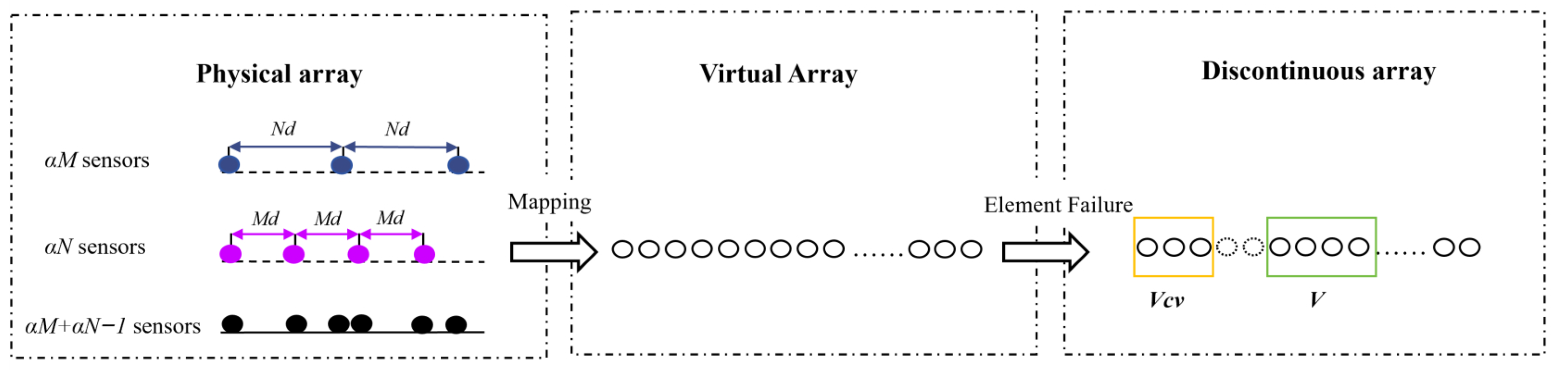
where “$\left|·\right|$” denotes the length (cardinality) of an array. Let ${\widehat{\mathit{v}}}_k$ represent the sparse estimation result obtained after the k-th iteration in the SSR process. The schematic diagram illustrating the selection principle for $\mathit{V}$ and ${\mathit{V}}_{cv}$ is shown in Figure 3.

Figure 3. Schematic diagram of V and Vcv selection.

The iteration error is

$${\epsilon }_k^s={∥\mathit{p}-{\widehat{\mathit{p}}}_k∥}_2^2,$$

(26)

and the validation error is

$${\epsilon }_k^{cv}={∥{\mathit{V}}_{cv}-{\mathit{A}}_{cv}{\widehat{\mathit{p}}}_k∥}_2^2.$$

(27)

As the number of iterations increases, ${\epsilon }_k^{cv}$ gradually decreases; however, it starts to increase again when the recovered signal becomes overfitted. Therefore, the iteration is terminated when ${\epsilon }_k^{cv}$ reaches its minimum value, which can be formulated as

$$\widehat{k}=arg\underset{k}{min}{\epsilon }_k^{cv},k=1,2,\dots ,E$$

(28)

where E denotes the maximum number of iterations. The MMP algorithm based on fragment array data validation is outlined in Algorithm 1. Here, ${\mathit{W}}^0$ represents the initial set of candidate paths, and ${\mathit{W}}^k=w_k^1,w_k^2,\dots ,w_k^u$ denotes the set of remaining candidate paths at the k-th iteration, where $w_k^u$ refers to the u-th index set among them. The variable r indicates the residual error associated with each candidate path during the selection process.

The basic workflow of the algorithm can be summarized as follows: first, based on $\mathit{V}$ and $\mathit{A}$, the MMP algorithm is used to obtain the optimal reconstruction path combination that minimizes the reconstruction residual; second, the sparse solution for each iteration is derived from the optimal reconstruction path set; finally, using fragment co-array validation, the optimal solution that minimizes the fragment co-array validation residual ${\epsilon }_k^{cv}$ is obtained based on ${\mathit{V}}_{cv}$ and ${\mathit{A}}_{cv}$.

The motivation, derivation, and assumptions for the specific steps of the algorithm are as follows:

Step 1: Initialization. The motivation is to define the initial state before the iteration begins:

$k=0$: Iteration counter.

${\mathit{W}}^0=\{\varnothing \}$: Candidate support set.

$r^0=\mathit{V}$: Initial residual. Since there is no reconstructed signal initially, the residual equals $\mathit{V}$.

${\epsilon }_0^{cv}$: Squared norm of the validation signal ${\mathit{V}}_{\mathrm{cv}}$.

The derivation is based on the definition of the residual, which is the difference between the observed value and the reconstructed value. It is assumed that the initial residual $r^0$ contains all the information of the sparse signal $\widehat{\mathit{p}}$, and the maximum number of iterations E is not less than the true sparsity of $\widehat{\mathit{p}}$.

Step 2: While loop. The motivation is to control the iteration termination condition, where each iteration corresponds to an increase in the support set size by 1, continuing until the maximum iteration count E is reached. The derivation is that MMP is a greedy iterative column selection algorithm, where each iteration expands the support set of the sparse signal by one element. The assumption is the true sparsity of $\widehat{\mathit{p}}$ does not exceed E.

Step 3–4: Iteration initialization and traversing candidate support sets from the previous round. The motivation is that when starting a new iteration, reset the current round’s candidate support set counter u and candidate set ${\mathit{W}}^k$ to prepare for generating new multi-path candidates. By expanding new paths based on all candidate support sets from the previous round ${\mathit{W}}^{k-1}$, this approach avoids local optima inherent in single-path matching pursuit.

The derivation basis is that each iteration must independently generate the candidate support sets for the current round. Multi-path expansion can cover more potential support set combinations, thereby increasing the probability of identifying the true support set of $\widehat{\mathit{p}}$. The assumption the candidate support sets from the previous round include candidates that are close to the true support set.

Step 5: Selecting the column most correlated with the residual. The motivation is to choose the column from the sensing matrix $\mathit{A}$ that has the largest inner product with the residual $r_{k-1}^m$ from the previous round. This derivation is based on the principle that the residual has a higher correlation with the columns of the true support set. The underlying assumption is that the sensing matrix $\mathit{A}$ satisfies the Restricted Isometry Property, ensuring low correlation between columns, and that the inner product between a true column and the residual is significantly greater than that of a noise column.

Step 6: Cycling to generate F candidate paths. The motivation is to generate F candidate support set paths per iteration, balancing the coverage of the true support set with computational complexity. The derivation is based on the premise that F is a preset number of paths, controlling the quantity of candidates in each iteration. The assumption is that the chosen value of F can cover a sufficient number of candidates.

Step 7: Extend the temporary support set. This step merges the candidate support set $w_{k-1}^m$ from the previous round with the newly selected column $o^{\prime }$ to generate a temporary support set. The derivation is based on the greedy algorithm, which adds one element to the support set in each iteration.

Step 8: Verify path uniqueness. The motivation is to avoid duplicate candidate support sets and reduce redundant computations. This is derived from the principle that duplicate paths do not provide new information. Ensuring the uniqueness of candidate support sets can lower the algorithm’s complexity without compromising the coverage of the true support set.

Step 9–10: Recording candidate support set motivation. The current round’s candidate counter u is updated, and the unique temporary support set $w^{\prime }$ is added to the current round’s candidate set ${\mathit{W}}^k$. This derivation is based on the principle of uniformly managing all candidate support sets for the current round, thereby preparing for subsequent solution steps.

Step 11: Solving for the sparse signal of the candidate support set. The motivation is to use the pseudo-inverse method to solve for the sparse signal once the candidate support set $w_k^u$ is known. This approach is derived from the fact that the pseudo-inverse provides the least squares solution to an underdetermined system of linear equations. The assumption here is that the submatrix ${\mathit{A}}_{w_k^u}$, corresponding to the candidate support set, is full column rank.

Step 12: Update the residual. The motivation is that the residual, defined as the difference between the original signal and the reconstructed signal from the candidate support set, serves as a measure of the reconstruction effectiveness for that candidate. This derivation is based on the definition of the residual in Equation (26), where a smaller residual indicates better reconstruction performance of the candidate support set.

Step 18: Select the candidate support set with the smallest residual. The motivation is that the candidate support set with the smallest residual has the highest match between its reconstructed signal and $\mathit{V}$, making it more likely to approximate the true support set. This derivation is based on Equation (26), where the core objective of sparse recovery is to minimize the residual.

Step 19: Solve for the sparse signal of each candidate. The motivation is to use the pseudo-inverse to solve for the corresponding sparse signal based on the selected candidate support set. The derivation follows the same pseudo-inverse solution logic as in Step 11.

Step 20: Calculate the verification error. The motivation is to combine fragmented co-array signals for validation to filter out false solutions. The derivation is based on Equation (27), where the fragmented array signals serve as validation signals.

Algorithm 1 MMP Based on Fragment Array Data Validation For Co-array.
Input: $\mathit{V}$, ${\mathit{V}}_{\mathrm{cv}}$, $\mathit{A}$, ${\mathit{A}}_{\mathrm{cv}}$, search path number F and maximum number of iterations E
1:  Initialization: $k=0$, ${\mathit{W}}^0=\{\varnothing \}$, $r^0=\mathit{V}$, ${\epsilon }_0^{cv}={\parallel {\mathit{V}}_{\mathrm{cv}}\parallel }_2^2$
2:  while $k<E$ do
3:        $k=k+1$, $u=0$, ${\mathit{W}}^k=\varnothing$
4:        for $m=1$ to $\left|W^{k-1}\right|$ do	(Equations (22) and (24))
5:              $o^{\prime }=argmax{∥{\left({\mathit{A}}^H{r}_{k-1}^m\right)}_o∥}_2^2$	(F candidate paths)
6:              for $n=1$ to F do
7:                    $w^{\prime }=w_{k-1}^m\cup \left\{o_n^{\prime }\right\}$	(Temporary path)
8:                    if $w^{\prime }\notin {\mathit{W}}^k$ then	(Check if the path exists)
9:                          $u=u+1$
10:                          $w_k^u=w^{\prime }$
11:                          ${\mathit{W}}^k={\mathit{W}}^k\cup \left\{w_k^u\right\}$
12:                          ${\widehat{\mathit{p}}}_k^u={\mathit{A}}_{w_k^u}^{†}\mathit{V}$	(Solve the candidate path)
13:                          ${\mathit{r}}_k^u=\mathit{V}-{\mathit{A}}_{w_k^R}{\widehat{\mathit{p}}}_k^u$	(Equation (26))
14:                    end if
15:              end for
16:       end for
17: end while
18: $w_D^{\widehat{u}}=arg{min}_n{∥r_E^n∥}_2^2,n=1,2,\dots ,u$	(Equation (26))
19: ${\widehat{\mathit{p}}}_k={\widehat{\mathit{p}}}_k^{\widehat{u}}={\mathit{A}}_{w_k^{\widehat{u}}}^{†}V,k=1,2,\dots ,E$	(Iterative solution)
20: ${\epsilon }_k^{cv}={∥{\mathit{V}}_{cv}-{\mathit{A}}_{cv}{\stackrel{\mathit{p}}{^}}_k∥}_2^2,k=1,2,\dots ,E$	(Equation (27))
21: $\widehat{k}=arg{min}_k{\epsilon }_k^{cv},k=1,2,\dots ,E$	(Equation (28))
Output: ${\widehat{p}}_k={\widehat{p}}_{\widehat{k}}$

Step 21: Select the solution with the minimum validation error. The motivation is to choose the solution that satisfies the criterion of having the smallest validation error. This derivation is based on Equation (28), where the solution with the minimum validation error is considered the most reliable. The assumption is that the segmented array signal ${\mathit{V}}_{\mathrm{cv}}$ can accurately reflect the true information of the co-array signal. By taking the minimum validation error of the segmented array as the convergence criterion, the algorithm is terminated precisely when the solution achieves the lowest reconstruction error. This approach removes the necessity of depending on external parameters such as noise variance or sparsity to determine the stopping point.

4. Simulation Analysis

4.1. Simulation Comparison Under Normal Operating Conditions of Array Elements

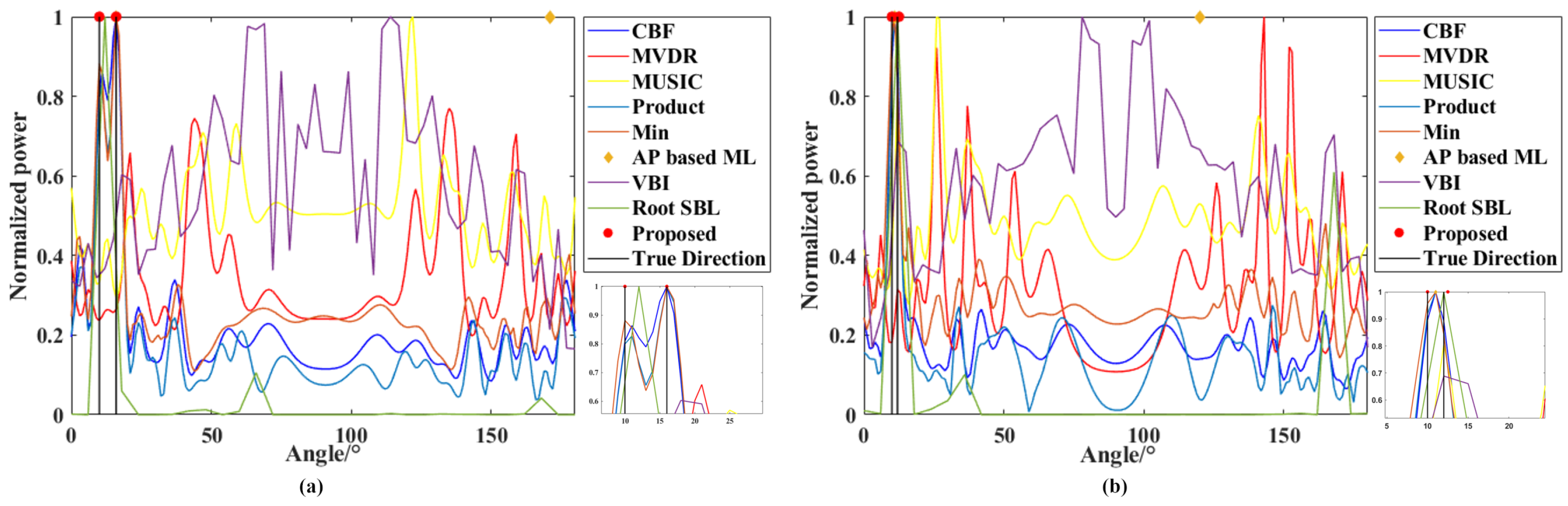
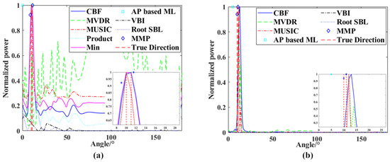
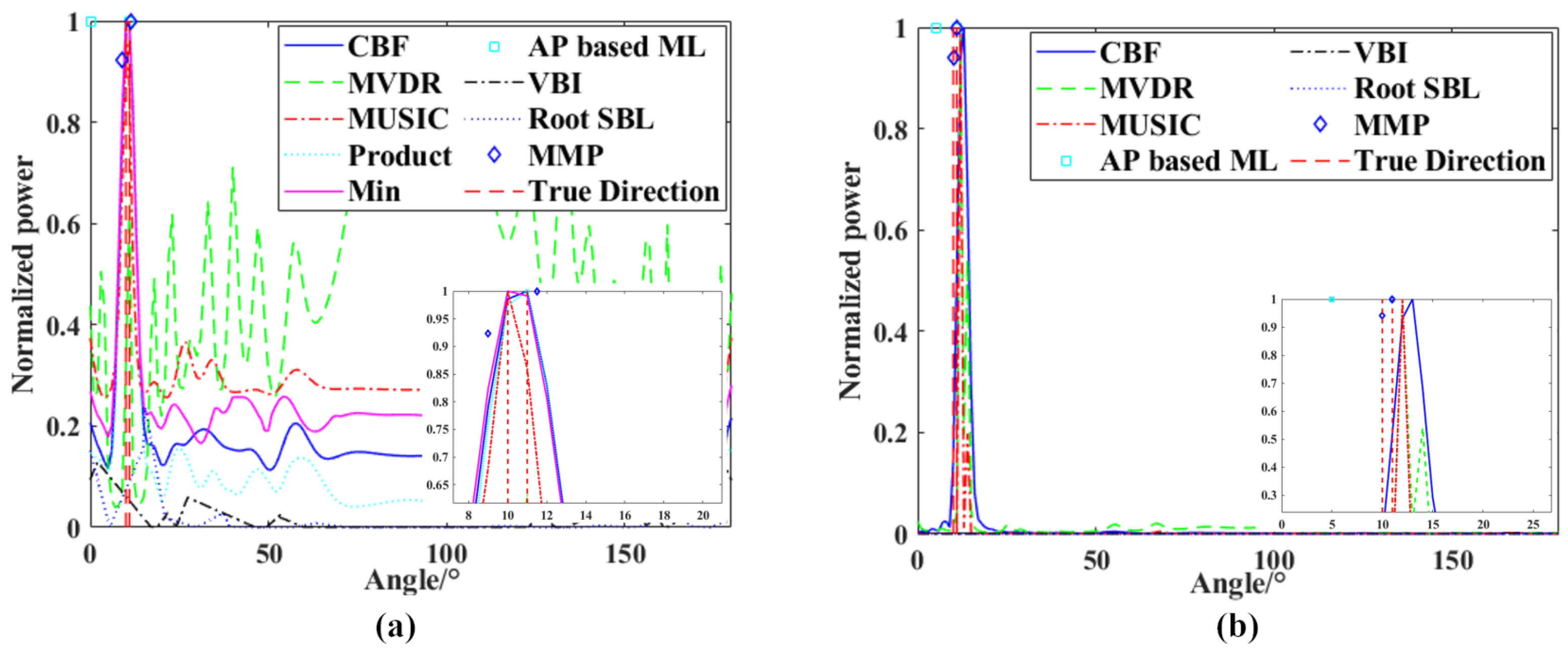
Figure 4 presents a single-trial DOA estimation result on the continuous co-array from the coprime array extended using the coprime minimum disordered pair. In this section, several methods are included for comparison: Conventional Beamforming (CBF), Minimum Variance Distortionless Response (MVDR), Multiple Signal Classification (MUSIC), robust processing methods such as Product and Min, and the classical parameter estimation technique Alternating Projection-based Maximum Likelihood Estimation (AP-based ML) [36,37]. Additionally, sparse signal reconstruction (SSR) methods including Root Sparse Bayesian Learning (Root SBL) [38] and Variational Bayesian Inference for Real-valued Sparse Bayesian Learning (VBI) [39] are also considered. In the Figure 4, the proposed method refers to the classical MMP algorithm applied to the co-array under the extended scheme presented in this paper.

Figure 4. Comparison results of algorithms. (a) The targets come from 10° and 16°. (b) The targets come from 10° and 12°.

In the simulation, we set $M=2$ and $N=3$ for the coprime array, with an expansion factor of $\alpha =4$. The signal-to-noise ratio (SNR) is $-10$ dB, and the number of signal snapshots is 10. The predefined search path is set to 6, and the maximum number of iterations is set to 4. In Figure 4a, two targets impinge on the coprime array from directions 10° and 16°, respectively. It can be observed that the CBF, Product, and Min methods are able to distinguish between the two directions, whereas MVDR and MUSIC perform poorly due to the low SNR and limited snapshot data. Repeated experiments indicate that the performance of AP-based ML and VBI is highly sensitive to the number of snapshots, with algorithmic stability emerging only after a sufficient number of snapshots is reached. Root SBL, on the other hand, is more sensitive to SNR and demonstrates improved performance even under low snapshot conditions when the SNR is high.

When the targets are located more closely, at 10° and 12° as shown in Figure 4b, the CBF, Product, Min, and Root SBL methods fail to resolve the two sources. In contrast, the method proposed in this paper successfully distinguishes the two azimuth angles and accurately estimates the true directions of the targets.

4.2. Comparative Simulation Analysis Under Array Element Failure Conditions

4.2.1. Continuous and Uninterrupted Co-Array Configuration

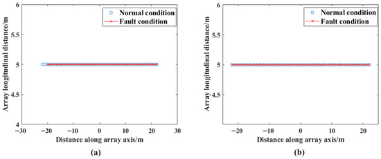
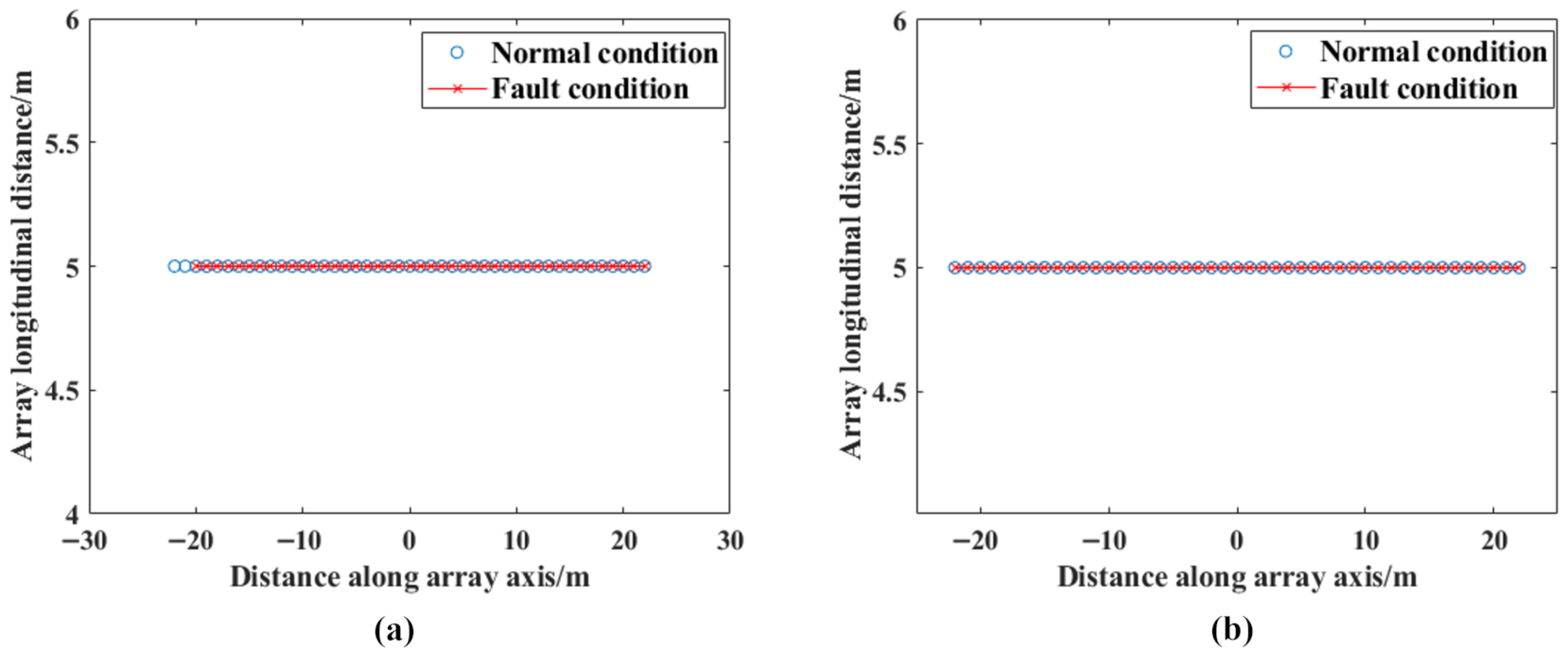
This section evaluates the performance of the SSR method in both the physical array and co-array domains, considering the presence of faulty array elements. For parameters $M=2$, $N=3$, and array expansion factor $\alpha =4$, the corresponding co-array is shown in Figure 5. The blue circles represent the co-array generated under normal operating conditions with all array elements functioning, while the red stars indicate the co-array resulting from a sensor malfunction. In this paper, the first sensor is indexed as 1. For instance, if element 1 malfunctions, its corresponding co-array element is missing, leading to a reduced co-array size. In contrast, if sensor 2 malfunctions, the co-array remains continuous and its size is unaffected.

Figure 5. The comparison of generated co-array between when all array elements are in normal working condition and when sensor failures occur. (a) Fault in sensor number 1. (b) Fault in sensor number 2.

Figure 6 presents a comparison of SSR methods applied to the physical array and co-array under faulty element conditions. The predefined search path is set to 6, and the maximum number of iterations is set to 4. In Figure 6a, due to the failure of physical array elements, the originally continuous array becomes discontinuous, leading to significant deviations in the processing results of conventional methods based on uniform linear arrays. Although both CBF and Min output high spatial spectra at the target directions, the difference in output between the two directions is small, making it practically difficult to distinguish the two targets. As shown in Figure 6b, it is evident that sensor failures have minimal impact on SSR performance in the co-array domain. Specifically, when sensor 1 fails, the co-array with 45 elements loses data from only two elements.

Figure 6. SSR results of array element failure situation. (a) SSR results in the physical array domain. (b) SSR results in the co-array domain.

4.2.2. The Continuity of the Co-Array Is Altered

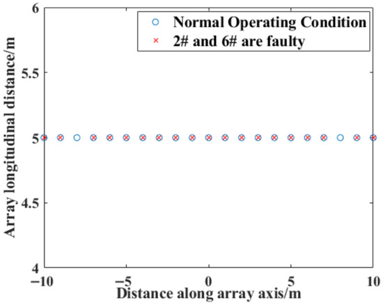
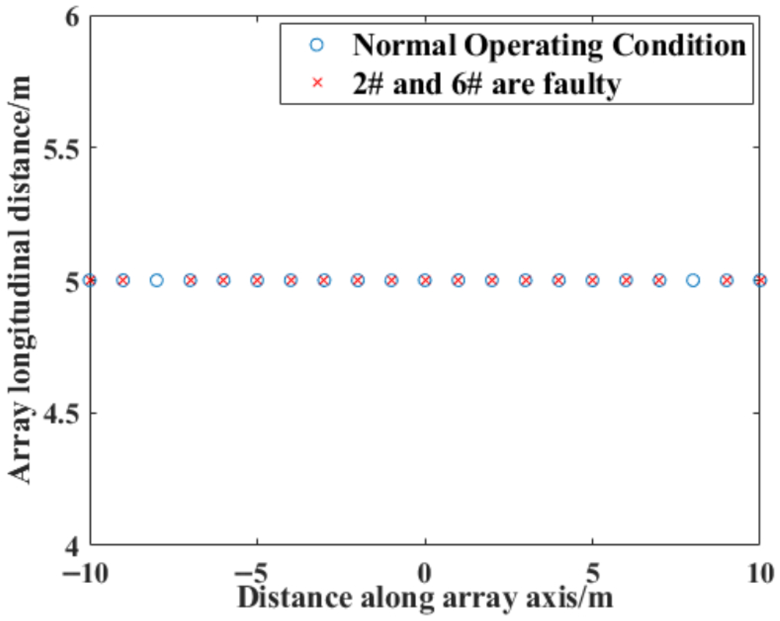
In some situations, malfunctioning elements cause a distortion in the covariance data, resulting in “holes” within the co-array and breaking the continuity of the originally contiguous array. For the parameters $M=2$, $N=3$, and an array expansion factor $\alpha =2$, the co-array generated by coprime array expansion is inherently continuous. However, when the second and sixth array elements malfunction, holes will arise in the previously continuous co-array, thereby leading to discontinuities.

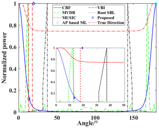
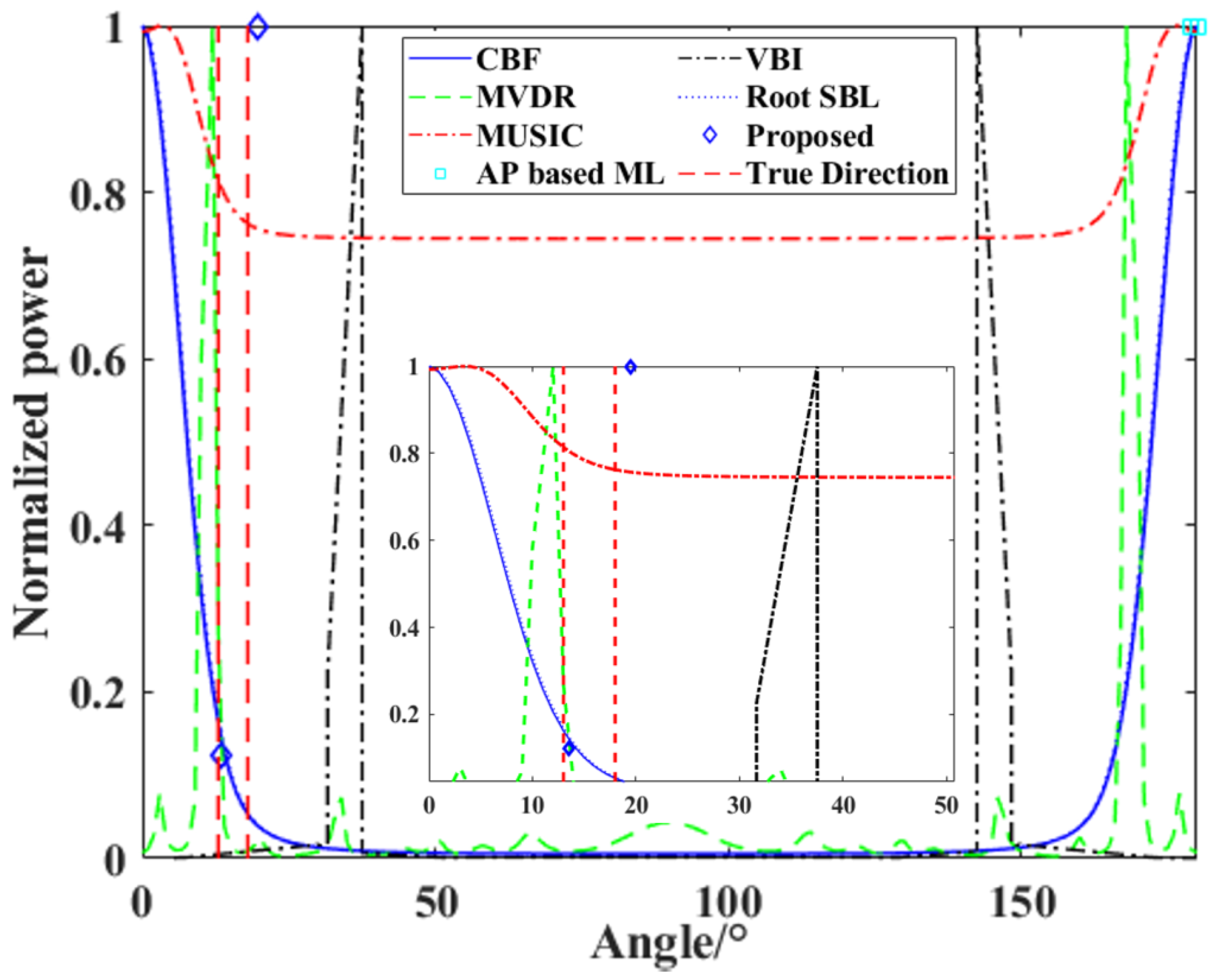
The discontinuous array scenario is illustrated in Figure 7, where the target directions are 13° and 18°, the SNR is −10 dB, and 10 snapshots are used. As demonstrated in Figure 8, despite the presence of discontinuities in the co-array, the proposed algorithm effectively recovers the co-array signals and accurately estimates the DOA. This confirms the robustness of the method in handling discontinuous co-arrays.

Figure 7. Comparison of the co-array in normal condition and the discontinuous array resulting from partial array sensors failure.

Figure 8. SSR results of discontinuous co-array signals obtained due to array sensor failures.

4.3. MSE Under Different SNRs and Snapshot Numbers

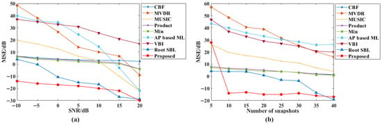
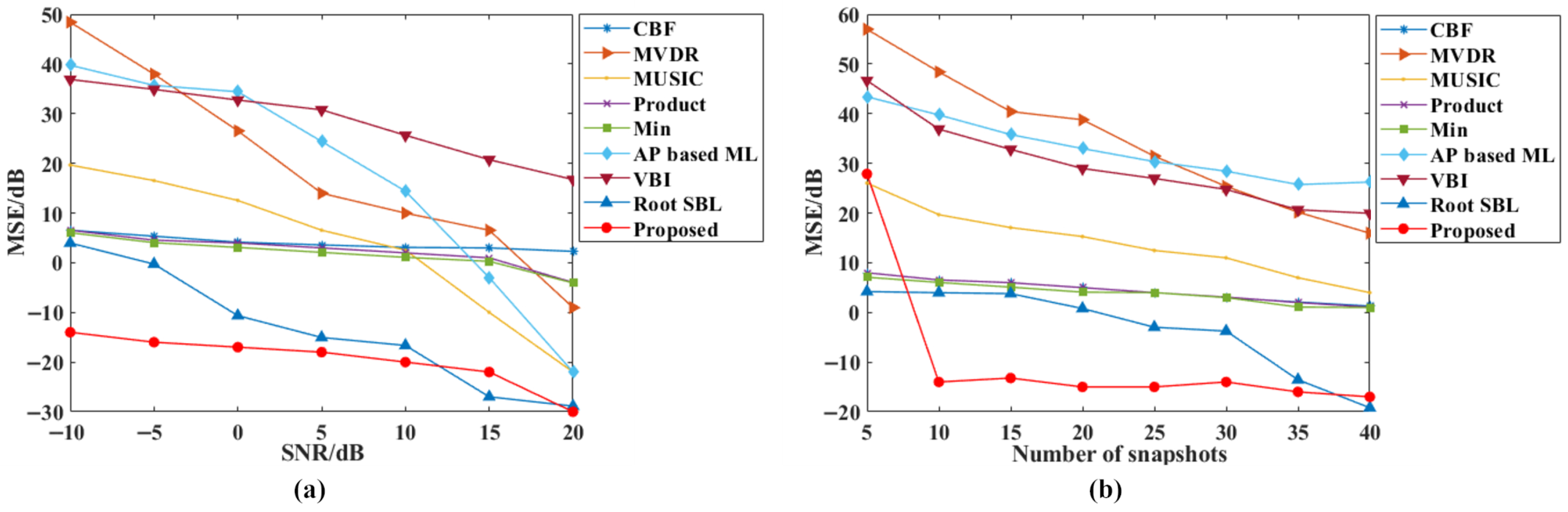
This section examines how the mean square error (MSE) of the proposed method changes with different SNRs and snapshot numbers. Here $M=2$, $N=3$, and an array expansion factor $\alpha =6$. The target directions are 20° and 23°. The co-array is interrupted when sensors 3, 4, 22, and 23 are set as faulty elements. The verification array is a co-array fragment with the length of 5 elements. The DOA estimation performance of different algorithms is evaluated using the MSE, which is described as

$$MSE={\displaystyle \frac{1}{IK}}\sum _{i=1}^I\sum _{k=1}^K{({\widehat{\theta }}_k\left(i\right)-{\theta }_k)}^2$$

(29)

where ${\widehat{\theta }}_k\left(i\right)$ denotes the DOA estimate of ${\theta }_k$ in the ith independent trial, and I and K represent the total number of Monte Carlo experiments and the number of signal sources, respectively.

When analyzing the MSE, the number of signal snapshots is fixed at 10 while the SNR varies. The statistical results in Figure 9 are based on 1000 independent trials. As shown in Figure 9a, the MSE decreases as the SNR increases. Figure 9b illustrates the MSE variation of the proposed method with different numbers of signal snapshots, where the SNR is fixed at −10 dB and other conditions remain unchanged. It is observed that the MSE stabilizes once the number of snapshots exceeds 15. Although the MSE of other methods also gradually decreases with increasing SNR and snapshot count, their overall performance remains inferior.

Figure 9. The mean squared error (MSE) of methods. (a) The relationship between MSE and SNR. (b) The relationship between MSE and signal snapshots.

4.4. Sensitivity Analysis to Sensor Position Errors

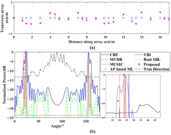
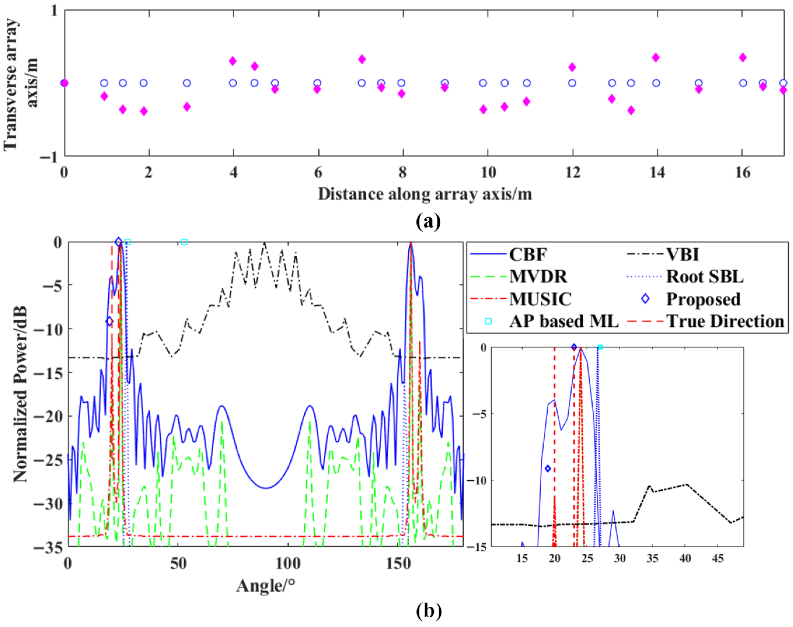
This section investigates the impact of sensor position errors on the proposed method to evaluate its robustness against signal mismatch. We assume that the sensors in the coprime array have random position errors with a mean magnitude of $15\%$ relative to the unit spacing. The simulation settings follow those in Section 4.3, with an SNR of −5 dB and 100 signal snapshots. The target directions are set at 20° and 23°.

As shown in Figure 10a, the ideal position of the array element is indicated by a blue circle, and the actual position of the array element is indicated by a pink diamond. As shown in Figure 10b, the performance of CBF, MVDR, and MUSIC algorithms degrades under array position errors, exhibiting spurious mirror peaks phenomena.The VBI algorithm fails, and both the RooT SBL and AP-based ML algorithms produce incorrect bearing estimation results. The proposed algorithm still maintains correct DOA estimation and achieves superior resolution capability, demonstrating its enhanced robustness under such mismatch conditions.

Figure 10. Algorithm performance when there are errors in the position of the array. (a) Array configuration with and without position error. (b) The target directions are 20° and 23°.

5. Sea Trial Data Analysis

This section evaluates the proposed method using two datasets obtained from sea trials. The experiment employed a 31-element scalar array with 2.5 m spacing between elements, deployed on the seabed at a depth of 20 m. The target was a test vessel. Acoustic data were recorded over 20 min within the frequency band of 200–350 Hz, at a sampling rate of 10 kHz.

In light of the robustness requirements for practical engineering applications, as discussed in Section 4.1 and Section 4.3, the Min algorithm is adopted for comparison in the physical array domain, while CBF is used in the co-array domain.

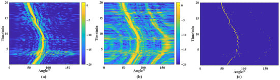
The coprime array configuration is defined by parameters $M=2$, $N=3$, and an expansion factor $\alpha =5$, resulting in a continuous co-array with 57 elements. The predefined search path is set to 6, and the maximum number of iterations is set to 4. Figure 11a presents the Bearing-Time Recording (BTR) result obtained using the Min algorithm. The target’s bearing trajectory is tracked stably throughout the measurement period. Figure 11b shows the result of applying CBF in the co-array domain. Due to the rank deficiency of the co-array covariance matrix, CBF requires spatial smoothing, which increases computational complexity and may introduce false peaks in bearing estimation.

Figure 11. BTR results from sea trial data, demonstrating that sensor failure does not disrupt co-array continuity. (a) Min method in the physical array domain. (b) CBF method in the co-array domain. (c) Proposed method in the co-array domain.

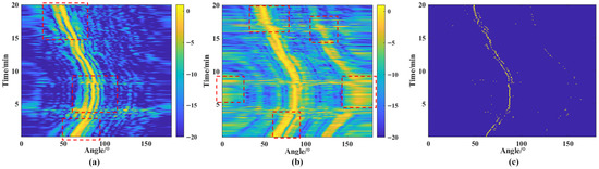
In contrast, Figure 11c illustrates the BTR result of the proposed method. During the experiment, the 22nd sensor was identified as faulty. Nevertheless, the algorithm effectively preserves the continuity of the co-array, ensuring that the failure does not compromise the signal reconstruction. As a result, DOA estimation can still be accurately performed using the SSR method based on the remaining continuous co-array elements, demonstrating the method’s robustness to sensor malfunction in real-world scenarios. To further validate the effectiveness of the proposed method, we manually designated the 3rd, 4th, 18th, and 19th sensors as faulty, thereby disrupting the originally continuous co-array of 57 elements. Figure 12 presents a comparison among the Min algorithm in the physical array domain, the CBF method using 45 valid co-array elements, and the proposed method employing fragment array data validation based on a co-array segment of 5 elements.

Figure 12. BTR results for the sea experiment data (the sensor damage breaks the continuity of the co-array). (a) Min in the physical array domain. (b) CBF in the co-array domain. (c) The proposed method.

When only a few sensors are faulty, the Min algorithm maintains a certain level of robustness, as shown in Figure 11a. However, as the number of faulty elements increases, its performance deteriorates significantly, resulting in ambiguous estimations and false target detections—highlighted by the red boxes in Figure 12a.

Comparing Figure 11b and Figure 12b, it is evident that a reduction in valid co-array elements introduces increased background interference and erroneous direction estimates in the target trajectory produced by the CBF method. This is further reflected by a noticeable increase in beamwidth, as indicated by the red boxes in Figure 12b, ultimately compromising the DOA estimation accuracy.

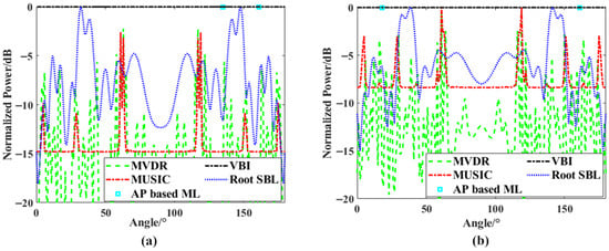
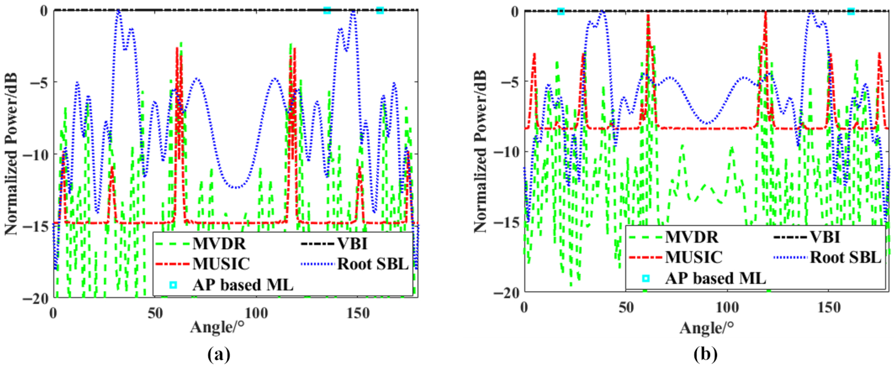
Although the results shown in Figure 12c indicate a slight degradation in clarity compared to Figure 11c, the proposed method based on fragment array data validation still delivers consistent and reliable trajectory estimations, demonstrating strong resilience under discontinuous co-array conditions. Figure 13 presents the time slice results of the comparison methods corresponding to the two sea trial data processing sessions. It can be observed that the MVDR and MUSIC algorithms exhibit false peak targets, the Root SBL and AP-based ML algorithms show high-amplitude outputs in non-target directions, and the VBI algorithm fails. The results are consistent with the simulation.

Figure 13. Comparison results of other algorithms for sea experiment data. (a) The situation where sensor damage does not compromise the continuity of the co-array. (b) The situation where sensor damage breaks the continuity of the co-array.

6. Conclusions

Coprime arrays have attracted considerable interest due to their ability to achieve high-resolution and stable beamforming in the physical array domain, as well as offering increased degrees of freedom (DoF) for target detection in the co-array domain. In the context of underwater acoustics, there is an urgent demand for array signal processing algorithms that can deliver high resolution while remaining effective with a limited number of snapshots. Addressing these practical engineering requirements, this paper investigates sparse signal recovery (SSR) methods in the co-array domain of coprime arrays for underwater applications.

There are two primary reasons for the formation of holes in the virtual array of coprime arrays: (1) Holes can arise when the coprime array is extended based on its initial configuration; (2) Physical element failures can also lead to holes in the co-array. To address the first scenario involving holes, this paper proposes an extension scheme based on the coprime minimum disordered pair. It is discussed and demonstrated that, under this extension method, the resulting co-array remains continuous, i.e., free of holes. For the second scenario, even if the extension scheme ensures a hole-free original co-array, fractures in the co-array due to physical element failures in practical settings cannot be entirely avoided. To address these issues, a novel SSR method based on fragment array data validation is introduced. This approach enables effective sparse recovery when the co-array is discontinuous, maximizing the utilization of available array data. The proposed algorithm demonstrates superior robustness to sensor failures compared to methods operating solely in the physical array domain and mitigates information loss caused by co-array interruptions.

Through extensive simulations and sea trial experiments, the proposed method is shown to significantly enhance spatial resolution and maintain reliable DOA estimation performance under sensor malfunctions. The algorithm offers a practical solution for reducing data degradation in underwater coprime arrays during deployment and operation, especially in scenarios involving large-scale array damage or maintenance-related limitations. It effectively preserves high-precision DOA estimation capabilities in the presence of both small- and large-scale co-array discontinuities.

References

- Moffet, A. Minimum-redundancy linear arrays. IEEE Trans. Antennas Propag. 1968, 16, 172–175. [Google Scholar] [CrossRef] [Scilit]
- Bloom, G.S.; Golomb, S.W. Applications of numbered undirected graphs. Proc. IEEE 1977, 65, 562–570. [Google Scholar] [CrossRef] [Scilit]
- Sheng, X.; Lu, D.; Li, Y.; de Lamare, R.C. Enhanced MISC-based sparse array with high uDOFs and low mutual coupling. IEEE Trans. Circuits Syst. II Express Briefs 2023, 71, 972–976. [Google Scholar] [CrossRef] [Scilit]
- Yang, T.; Ye, Z. Array gain of coprime arrays. J. Acoust. Soc. Am. 2019, 146, EL306–EL309. [Google Scholar] [CrossRef] [Scilit]
- Di Martino, G.; Iodice, A. Passive beamforming with coprime arrays. IET Radar Sonar Navig. 2017, 11, 964–971. [Google Scholar] [CrossRef] [Scilit]
- Berman, A.; Clay, C. Theory of Time-Averaged-Product Arrays. J. Acoust. Soc. Am. 1957, 29, 805–812. [Google Scholar] [CrossRef] [Scilit]
- Vaidyanathan, P.P.; Pal, P. Sparse sensing with co-prime samplers and arrays. IEEE Trans. Signal Process. 2010, 59, 573–586. [Google Scholar] [CrossRef] [Scilit]
- Tan, Z.; Nehorai, A.; Eldar, Y.C. Continuous sparse recovery for direction of arrival estimation with co-prime arrays. In Proceedings of the 2014 IEEE 8th Sensor Array and Multichannel Signal Processing Workshop (SAM), A Coruna, Spain, 22–25 June 2014; IEEE: Piscataway, NJ, USA, 2014; pp. 393–396. [Google Scholar]
- Liu, Y.; Buck, J.R. Detecting Gaussian signals in the presence of interferers using the coprime sensor arrays with the min processor. In Proceedings of the 2015 49th Asilomar Conference on Signals, Systems and Computers, Pacific Grove, CA, USA, 8–11 November 2015; IEEE: Piscataway, NJ, USA, 2015; pp. 370–374. [Google Scholar]
- Liu, Y.; Buck, J.R. Spatial spectral estimation using a coprime sensor array with the min processor. In Proceedings of the 2016 IEEE Sensor Array and Multichannel Signal Processing Workshop (SAM), Rio de Janeiro, Brazil, 10–13 July 2016; IEEE: Piscataway, NJ, USA, 2016; pp. 1–5. [Google Scholar]
- Liu, Y.; Buck, J.R. Gaussian source detection and spatial spectral estimation using a coprime sensor array with the min processor. IEEE Trans. Signal Process. 2017, 66, 186–199. [Google Scholar] [CrossRef] [Scilit]
- Adhikari, K.; Buck, J.R.; Wage, K.E. Beamforming with extended co-prime sensor arrays. In Proceedings of the 2013 IEEE International Conference on Acoustics, Speech and Signal Processing, Vancouver, BC, Canada, 26–31 May 2013; IEEE: Piscataway, NJ, USA, 2013; pp. 4183–4186. [Google Scholar]
- Adhikari, K.; Buck, J.R.; Wage, K.E. Extending coprime sensor arrays to achieve the peak side lobe height of a full uniform linear array. EURASIP J. Adv. Signal Process. 2014, 2014, 148. [Google Scholar] [CrossRef] [Scilit]
- Saadati Moghadam, G.; Beheshti Shirazi, A. Novel method for digital beamforming in co-prime sensor arrays using product and min processors. IET Signal Process. 2019, 13, 614–623. [Google Scholar] [CrossRef] [Scilit]
- Zhou, C.; Gu, Y.; Song, W.Z.; Xie, Y.; Shi, Z. Robust adaptive beamforming based on DOA support using decomposed coprime subarrays. In Proceedings of the 2016 IEEE International Conference on Acoustics, Speech and Signal Processing (ICASSP), Shanghai, China, 20–25 March 2016; IEEE: Piscataway, NJ, USA, 2016; pp. 2986–2990. [Google Scholar]
- Zhou, C.; Gu, Y.; He, S.; Shi, Z. A robust and efficient algorithm for coprime array adaptive beamforming. IEEE Trans. Veh. Technol. 2017, 67, 1099–1112. [Google Scholar] [CrossRef] [Scilit]
- Zhou, C.; Shi, Z.; Gu, Y.; Goodman, N.A. DOA estimation by covariance matrix sparse reconstruction of coprime array. In Proceedings of the 2015 IEEE International Conference on Acoustics, Speech and Signal Processing (ICASSP), South Brisbane, QLD, Australia, 19–24 April 2015; IEEE: Piscataway, NJ, USA, 2015; pp. 2369–2373. [Google Scholar]
- Zhou, C.; Shi, Z.; Gu, Y.; Zhang, Y.D. Coarray interpolation-based coprime array DOA estimation via covariance matrix reconstruction. In Proceedings of the 2018 IEEE International Conference on Acoustics, Speech and Signal Processing (ICASSP), Calgary, AB, Canada, 15–20 April 2018; IEEE: Piscataway, NJ, USA, 2018; pp. 3479–3483. [Google Scholar]
- Ortiz-Jiménez, G.; Coutino, M.; Chepuri, S.P.; Leus, G. Sparse sampling for inverse problems with tensors. IEEE Trans. Signal Process. 2019, 67, 3272–3286. [Google Scholar] [CrossRef] [Scilit]
- Liu, C.L.; Vaidyanathan, P. Tensor MUSIC in multidimensional sparse arrays. In Proceedings of the 2015 49th Asilomar Conference on Signals, Systems and Computers, Pacific Grove, CA, USA, 8–11 November 2015; IEEE: Piscataway, NJ, USA, 2015; pp. 1783–1787. [Google Scholar]
- Yang, X.; Wang, Y.; Chargé, P. Improved coprime linear array configuration for moving platform in DOA estimation. IEEE Commun. Lett. 2020, 25, 470–473. [Google Scholar] [CrossRef] [Scilit]
- Pan, Y.; Luo, G.Q. Efficient direction-of-arrival estimation via annihilating-based denoising with coprime array. Signal Process. 2021, 184, 108061. [Google Scholar] [CrossRef] [Scilit]
- Pal, P.; Vaidyanathan, P.P. Coprime sampling and the MUSIC algorithm. In Proceedings of the 2011 Digital Signal Processing and Signal Processing Education Meeting (DSP/SPE), Sedona, AZ, USA, 4–11 January 2011; IEEE: Piscataway, NJ, USA, 2011; pp. 289–294. [Google Scholar]
- Zheng, Z.; Huang, Y.; Wang, W.Q.; So, H.C. Direction-of-arrival estimation of coherent signals via coprime array interpolation. IEEE Signal Process. Lett. 2020, 27, 585–589. [Google Scholar] [CrossRef] [Scilit]
- Liu, C.L.; Vaidyanathan, P.; Pal, P. Coprime coarray interpolation for DOA estimation via nuclear norm minimization. In Proceedings of the 2016 IEEE International Symposium on Circuits and Systems (ISCAS), Montreal, QC, Canada, 22–25 May 2016; IEEE: Piscataway, NJ, USA, 2016; pp. 2639–2642. [Google Scholar]
- Wu, X.; Zhu, W.P.; Yan, J. A Toeplitz covariance matrix reconstruction approach for direction-of-arrival estimation. IEEE Trans. Veh. Technol. 2017, 66, 8223–8237. [Google Scholar] [CrossRef] [Scilit]
- Zhou, C.; Gu, Y.; Fan, X.; Shi, Z.; Mao, G.; Zhang, Y.D. Direction-of-arrival estimation for coprime array via virtual array interpolation. IEEE Trans. Signal Process. 2018, 66, 5956–5971. [Google Scholar] [CrossRef] [Scilit]
- Ma, P.; Li, J.; Xu, F.; Zhang, X. Hole-free coprime array for DOA estimation: Augmented uniform co-array. IEEE Signal Process. Lett. 2020, 28, 36–40. [Google Scholar] [CrossRef] [Scilit]
- Lai, X.; Zhang, X.; Han, S.; Ahmad, M. Multi-layer filled coprime arrays for DOA estimation with extended hole-free coarray. IEEE Trans. Veh. Technol. 2023, 73, 2621–2632. [Google Scholar] [CrossRef] [Scilit]
- Shaikh, A.H.; Liu, X. Super Fragmented Coprime Arrays for DOA Estimation. IEEE Signal Process. Lett. 2025, 32, 1825–1829. [Google Scholar] [CrossRef] [Scilit]
- Lai, X.; Zhang, X.; Zheng, W.; Li, J.; Zhou, F. Fragmented coprime arrays with optimal inter subarray spacing for DOA estimation: Increased DOF and reduced mutual coupling. Signal Process. 2024, 215, 109273. [Google Scholar] [CrossRef] [Scilit]
- Yan, F.G.; Li, X.; Meng, X.T.; Greco, M.S.; Gini, F. Lengthened Coprime Arrays with Hole-free Coarrays and Reduced Mutual Coupling. IEEE Signal Process. Lett. 2025, 32, 2509–2513. [Google Scholar] [CrossRef] [Scilit]
- Candès, E.J.; Romberg, J.; Tao, T. Robust uncertainty principles: Exact signal reconstruction from highly incomplete frequency information. IEEE Trans. Inf. Theory 2006, 52, 489–509. [Google Scholar] [CrossRef] [Scilit]
- Friedlander, B.; Weiss, A.J. Direction finding using spatial smoothing with interpolated arrays. IEEE Trans. Aerosp. Electron. Syst. 2002, 28, 574–587. [Google Scholar] [CrossRef] [Scilit]
- Li, W.; Li, Y.P.; Yu, W.H. On adaptive beamforming for coherent interference suppression via virtual antenna array. Prog. Electromagn. Res. 2012, 125, 165–184. [Google Scholar] [CrossRef] [Scilit]
- Hou, H.; Mao, X. Doa estimation of uncorrelated, partly correlated and coherent signals using alternating oblique projection. Radioengineering 2017, 26, 588–600. [Google Scholar] [CrossRef] [Scilit]
- Chen, J.C.; Hudson, R.E.; Yao, K. Maximum-likelihood source localization and unknown sensor location estimation for wideband signals in the near-field. IEEE Trans. Signal Process. 2002, 50, 1843–1854. [Google Scholar] [CrossRef] [Scilit]
- Dai, J.; Bao, X.; Xu, W.; Chang, C. Root sparse Bayesian learning for off-grid DOA estimation. IEEE Signal Process. Lett. 2016, 24, 46–50. [Google Scholar] [CrossRef] [Scilit]
- Dai, J.; So, H.C. Real-valued sparse Bayesian learning for DOA estimation with arbitrary linear arrays. IEEE Trans. Signal Process. 2021, 69, 4977–4990. [Google Scholar] [CrossRef] [Scilit]
- Hu, Y.; Yin, J.; Li, T.; Cao, J.; Zhang, L. High gain beamforming method in low-frequency band using virtual array migration. Appl. Acoust. 2025, 232, 110570. [Google Scholar] [CrossRef] [Scilit]
- Chavali, V.; Wage, K.E.; Buck, J.R. Coprime processing for the Elba Island sonar data set. In Proceedings of the 2014 48th Asilomar Conference on Signals, Systems and Computers, Pacific Grove, CA, USA, 2–5 November 2014; IEEE: Piscataway, NJ, USA, 2014; pp. 1864–1868. [Google Scholar]
- Chavali, V.; Wage, K.E.; Buck, J.R. Multiplicative and min processing of experimental passive sonar data from thinned arrays. J. Acoust. Soc. Am. 2018, 144, 3262–3274. [Google Scholar] [CrossRef] [Scilit] [PubMed]
- Chavali, V. Coprime and Nested Array Processing of the Elba Island Sonar Data Set. Master’s Thesis, University of Mumbai, Mumbai, India, 2017. [Google Scholar]
- Chen, X.; Zhang, H.; Lv, Y. Improving the beamforming performance of a vector sensor line array with a coprime array configuration. Appl. Acoust. 2023, 207, 109329. [Google Scholar] [CrossRef] [Scilit]
- Chan, Y. Underwater Acoustic Data Processing; Springer Science & Business Media: Berlin/Heidelberg, Germany, 2012; Volume 161. [Google Scholar]
- Sun, D.; Jia, Z.; Teng, T.; Ma, C. Robust high-resolution direction-of-arrival estimation method using DenseBlock-based U-net. J. Acoust. Soc. Am. 2022, 151, 3426–3436. [Google Scholar] [CrossRef] [Scilit] [PubMed]
- Sun, D.; Ma, C.; Mei, J.; Shi, W. Improving the resolution of underwater acoustic image measurement by deconvolution. Appl. Acoust. 2020, 165, 107292. [Google Scholar] [CrossRef] [Scilit]
- Liu, X.; Fan, J.; Sun, C.; Yang, Y.; Zhuo, J. High-resolution and low-sidelobe forward-look sonar imaging using deconvolution. Appl. Acoust. 2021, 178, 107986. [Google Scholar] [CrossRef] [Scilit]
- Zhang, H.; Gao, Z.; Fu, H. A high resolution random linear sonar array based MUSIC method for underwater DOA estimation. In Proceedings of the 32nd Chinese Control Conference, Xi’an, China, 26–28 July 2013; IEEE: Piscataway, NJ, USA, 2013; pp. 4592–4595. [Google Scholar]
- Van Trees, H.L. Optimum Array Processing: Part IV of Detection, Estimation, and Modulation Theory; John Wiley & Sons: Hoboken, NJ, USA, 2002. [Google Scholar]
- Vaidyanathan, P.; Pal, P. Theory of sparse coprime sensing in multiple dimensions. IEEE Trans. Signal Process. 2011, 59, 3592–3608. [Google Scholar] [CrossRef] [Scilit]
- Kulkarni, P.; Vaidyanathan, P.P. Weight-constrained sparse arrays for direction of arrival estimation under high mutual coupling. IEEE Trans. Signal Process. 2024, 72, 4444–4462. [Google Scholar] [CrossRef] [Scilit]
- Kwon, S.; Wang, J.; Shim, B. Multipath matching pursuit. IEEE Trans. Inf. Theory 2014, 60, 2986–3001. [Google Scholar] [CrossRef] [Scilit]
- Zhang, J.; Chen, L.; Boufounos, P.T.; Gu, Y. On the theoretical analysis of cross validation in compressive sensing. In Proceedings of the 2014 IEEE International Conference on Acoustics, Speech and Signal Processing (ICASSP), Florence, Italy, 4–9 May 2014; IEEE: Piscataway, NJ, USA, 2014; pp. 3370–3374. [Google Scholar]
Disclaimer/Publisher’s Note: The statements, opinions and data contained in all publications are solely those of the individual author(s) and contributor(s) and not of MDPI and/or the editor(s). MDPI and/or the editor(s) disclaim responsibility for any injury to people or property resulting from any ideas, methods, instructions or products referred to in the content. |
© 2026 by the authors. Licensee MDPI, Basel, Switzerland. This article is an open access article distributed under the terms and conditions of the Creative Commons Attribution (CC BY) license.