Symbolic Algorithm for Solving Nonlocal Boundary Value Problems for Systems of Ordinary Integrodifferential Equations

Abstract

Boundary value problems for systems of integrodifferential equations appear in many branches of science and engineering. Accuracy in modeling complex processes requires the specification of nonlocal boundary conditions, including multipoint and integral conditions. These kinds of problems are even harder to solve. In this paper, we present solvability criteria and a direct operator method for constructing the exact solution to systems of linear ordinary integrodifferential equations with general nonlocal boundary conditions. A symbolic algorithm is also proposed. Several examples are solved to demonstrate the effectiveness of the method. The results obtained are equally valid for nonlocal boundary value problems for systems of ordinary differential, loaded differential, and loaded integrodifferential equations.

1. Introduction

Boundary value problems for systems of linear and nonlinear ordinary differential equations, due to their occurrence in numerous applications in science and engineering, have been extensively studied by many researchers. Corresponding problems with nonlocal boundary conditions have also been investigated. Kiguradze [1] considered the following general boundary value problem for a system of linear ordinary differential equations

$$\begin{array}{ccc}\hfill {\displaystyle \frac{dx}{dt}}& =& P\left(t\right)x+q\left(t\right),\hfill \end{array}$$

(1)

$$\begin{array}{ccc}\hfill \mathit{l}\left(x\right)& =& c_0,\hfill \end{array}$$

(2)

where $P\in L([a,b];{\mathbf{R}}^{n\times n})$, $q\in L([a,b];{\mathbf{R}}^n)$, $c_0\in {\mathbf{R}}^n$ and $\mathit{l}:C([a,b];{\mathbf{R}}^n)\to {\mathbf{R}}^n$ is a continuous linear transformation, and the corresponding homogeneous system

$$\begin{array}{ccc}\hfill {\displaystyle \frac{dx}{dt}}& =& P\left(t\right)x,\hfill \end{array}$$

(3)

$$\begin{array}{ccc}\hfill \mathit{l}\left(x\right)& =& 0.\hfill \end{array}$$

(4)

He proved that Equations (1) and (2) are uniquely solvable if and only if

$$det\mathit{l}\left(Y\right)\ne 0,$$

(5)

where Y is the fundamental matrix of Equation (3) satisfying the condition

$$Y\left(a\right)=E,$$

where E is the identity matrix. If Equation (5) holds, then the solution x of Equations (1) and (2) has the representation

$$x\left(t\right)=x_0\left(t\right)+{\int }_a^{b}G(t,\tau )q\left(\tau \right)d\tau ,$$

where $x_0$ is the solution of Equations (2) and (3) and G is the Greens’ matrix of homogeneous Equations (3) and (4). These results are important and of practical use, as they are computationally efficient and can be easily implemented in modern computer algebra systems for constructing solutions to boundary value problems for differential equations.

Integrodifferential equations have many applications in biology, physics, engineering, chemical engineering and economics, and especially in population dynamics, epidemiology, hereditary mechanics, electromagnetic theory, viscoelasticity, nonlocal elasticity, heat transfer, fluid dynamics, automatic control, network theory, and elsewhere [2,3]. Integrodifferential equations (IDEs) involve a differential and an integral operator, and the state of the unknown function depends on its values at a point as well as on its previous and/or nonlocal spatial interactions, which are taken into account by the integral term. Boundary value problems for integrodifferential equations with nonlocal conditions have attracted increasing interest in recent years. The necessity and development of nonlocal boundary conditions in the modeling of complex physical situations are discussed in [4,5,6,7]. Due to the high mathematical complexity involved, numerical methods are mainly used to solve nonlocal boundary value problems. Approximate numerical methods for solving nonlocal boundary value problems for systems of Fredholm integrodifferential equations (FIDEs) can be found in [8,9,10,11], and the references therein. However, numerical methods lead to approximate solutions, require careful stability and error analysis, and provide less intuitive insight. Therefore, closed-form solutions are preferred whenever possible. Furthermore, the latter are also necessary for validating the former. The solvability and exact solution of general and some special boundary value problems for a single linear nth-order ordinary FIDE with nonlocal boundary conditions are investigated in [12,13,14,15]. An approach involving problem transformation and the use of generalized inverse operators to find solvability criteria and solutions to boundary value problems for systems of FIDEs is proposed in [16,17,18]. Also, another method involving the reduction in the system to the solution of a number of simpler differential systems is presented in [19]. The exact solution to systems of first-order FIDEs with constant coefficients and homogeneous general boundary conditions is studied in [20]. From the above analysis, it is understood that there is no direct method for the closed-form solution of boundary value problems for systems of FIDEs with variable coefficients and nonohomogeneous nonlocal boundary conditions. Finally, for the sake of completeness, although not studied here, reference is made to the research on the existence and uniqueness of solutions to classes of boundary value problems for fractional integrodifferential equations with nonlocal boundary conditions [21,22,23].

In this paper, we consider a general nonlocal boundary value problem for a system of linear ordinary FIDEs which is written in matrix form as   

$$\begin{array}{ccc}\hfill x^{\prime }\left(t\right)-A\left(t\right)x\left(t\right)-G\left(t\right)\eta \left(x\right)& =& f\left(t\right),a\le t\le b,\hfill \end{array}$$

(6)

$$\begin{array}{ccc}\hfill \theta \left(x\right)& =& c,\hfill \end{array}$$

(7)

where $x\left(t\right)={\left(\begin{array}{ccc}{x}_1\left(t\right)& \cdots & x_n\left(t\right)\end{array}\right)}^T$ is the $n\times 1$ vector of unknown functions, $x^{\prime }\left(t\right)={\displaystyle \frac{d}{dt}}x\left(t\right)={\left(\begin{array}{ccc}{x}_1^{\prime }\left(t\right)& \cdots & x_n^{\prime }\left(t\right)\end{array}\right)}^T$, $A\left(t\right)$, $G\left(t\right)$ are, respectively, $n\times n$ and $n\times m$ matrices of given functions, $\eta \left(x\right)={\left(\begin{array}{ccc}{\eta }_1\left(x\right)& \cdots & {\eta }_m\left(x\right)\end{array}\right)}^T$ is an $m\times 1$ vector of linear bounded functionals (definite integrals) valued on x, and $f\left(t\right)$ is an $n\times 1$ vector of given forcing functions. The $n\times 1$ vector $\theta \left(x\right)={\left(\begin{array}{ccc}{\theta }_1\left(x\right)& \cdots & {\theta }_n\left(x\right)\end{array}\right)}^T$ is a vector of linear bounded functionals of the type,

$$\theta \left(x\right)=\sum _{j=1}^{{\mathcal{l}}_1}{A}_{j}x\left(t_j\right)+\sum _{j=1}^{{\mathcal{l}}_2}{B}_j{\int }_{{\xi }_j}^{{\xi }_{j+1}}{C}_j\left(s\right)x\left(s\right)ds,$$

where $C_j\left(t\right)$ is an $n\times n$ matrix of functions, $A_j,B_j$ are $n\times n$ constant matrices, $a=t_1<t_2<\cdots <t_{{\mathcal{l}}_1-1}<t_{{\mathcal{l}}_1}=b$ and $a={\xi }_1<{\xi }_2<\cdots <{\xi }_{{\mathcal{l}}_2}<{\xi }_{{\mathcal{l}}_2+1}=b$, and $c={\left(\begin{array}{ccc}{c}_1& \cdots & c_n\end{array}\right)}^T$ is an $n\times 1$ vector of constants. We extend Kiguradze’s results to the class of Equations (6) and (7), and in particular we derive solvability criteria of the type as in Equation (5) and a formula for their solution in closed form. The analysis is based on the existence of the inverse differential operator in closed form, which essentially depends on the availability of the fundamental matrix Z of the homogeneous differential system $x^{\prime }-A\left(t\right)x=0$. The fundamental matrix can be computed analytically for systems with constant coefficients and for systems with special variable coefficient structures [24].

The proposed method is innovative in its design and scope compared to other works in the literature. It is a unified direct matrix approach for symbolic computation that can be applied to various classes of general boundary value problems that can be put in the form of Equations (6) and (7), such as boundary value problems for differential and integrodifferential equations as well as for loaded differential and loaded integrodifferential equations [25,26]. Symbolic computation is increasingly used in solving problems in many areas of mathematics, such as algebra, geometry and differential equations [27,28]. The proposed symbolic algorithm can be easily implemented in any available computer algebra system.

The paper is organized as follows: In Section 2, the problem is formulated in an operator form in a Banach space and some preliminary results are presented. The main results are given in Section 3 where two key theorems for the solvability of the problem are proved and a symbolic procedure for constructing the solution is presented. In Section 4, several examples are solved to demonstrate the application and effectiveness of the proposed technique. The conclusions are drawn in Section 5.

2. Preliminaries

Let $\mathbb{X}$ denotes a Banach space, namely the space of continuous functions $C[a,b]$ or the Lebesgue space $L_p(a,b)$, with $a,b\in \mathbb{R}$. Let ${\mathbb{X}}_n$ be the n-dimensional vector space of all column vectors $x\left(t\right)={\left(x_1\left(t\right),\dots ,x_n\left(t\right)\right)}^T$ with $x_i\left(t\right)\in \mathbb{X},i=1,\dots ,n$, and ${\mathbb{X}}_n^1$ denote the space of all x that have continuous first derivatives $C_n^1[a,b]$ or the Sobolev space $W_{p_n}^1(a,b)$.

Let ${\left[{\mathbb{X}}_n\right]}^{*}$ be the dual space of ${\mathbb{X}}_n$, i.e., the set of all linear bounded functionals ${\varphi }_i$ defined on ${\mathbb{X}}_n$. We denote by ${\varphi }_i\left(x\right)$ the value of ${\varphi }_i$ at $x\in {\mathbb{X}}_n$ and

$$\varphi \left(x\right)=\left(\begin{array}{c}{\varphi }_1\left(x\right)\\ ⋮\\ {\varphi }_n\left(x\right)\end{array}\right),\varphi \left(Z\right)=\left[\begin{array}{ccc}\varphi \left(z_1\right)& \cdots & \varphi \left(z_n\right)\end{array}\right],$$

where Z is $n\times n$ matrix of functions with the column vectors $z_1,\dots ,z_n\in {\mathbb{X}}_n$. Note that for any $n\times 1$ constant vector c,

$$\varphi \left(Zc\right)=\varphi \left(Z\right)c.$$

(8)

Throughout this paper, $I_n$ denotes the $n\times n$ identity matrix and 0 is used to denote the scalar zero and the all-zero vector or matrix, as appropriate, without confusion.

Let the operator $\mathcal{A}:{\mathbb{X}}_n\to {\mathbb{X}}_n$, $\mathfrak{D}\left(\mathcal{A}\right)$ and $\mathfrak{R}\left(\mathcal{A}\right)$ be the domain and range of this operator, respectively. The operator $\mathcal{A}$ is said to be injective or uniquelly solvable if for all $x,y\in \mathfrak{D}\left(\mathcal{A}\right)$ such that $\mathcal{A}x=\mathcal{A}y$, it follows that $x=y.$ Recall that a linear operator $\mathcal{A}$ is injective if and only if $ker\mathcal{A}=\left\{0\right\}.$ The operator $\mathcal{A}$ is called surjective or everywhere solvable if $\mathfrak{R}\left(\mathcal{A}\right)={\mathbb{X}}_n.$ The operator $\mathcal{A}$ is called bijective if $\mathcal{A}$ is both injective and surjective.

Definition 1. 

The operator $\mathcal{A}$ is said to be correct if $\mathcal{A}$ is bijective and its inverse ${\mathcal{A}}^{-1}$ is bounded on $\mathfrak{R}\left(\mathcal{A}\right)={\mathbb{X}}_n$.

Definition 2. 

The problem $\mathcal{A}x=f,f\in {\mathbb{X}}_n,$ is said to be well posed and hence uniquely and everywhere solvable, if the operator $\mathcal{A}$ is correct.

Lemma 1. 

Let the operator $\mathcal{A}:{\mathbb{X}}_n\to {\mathbb{X}}_n$ be defined by

$$\mathcal{A}x=x^{\prime }-A\left(t\right)x,\mathfrak{D}\left(\mathcal{A}\right)=\left\{x\in {\mathbb{X}}_n^1\right\},$$

(9)

where $A\left(t\right)$ is a $n\times n$ matrix of functions $a_{ij}\left(t\right)\in \mathbb{X},i,j=1,\dots ,n$, and the boundary functional vector $\widehat{\theta }\in {\left[{\mathbb{X}}_n\right]}^{*}$. Let $Z\left(t\right)$ be a fundamental matrix of the homogeneous equation $\mathcal{A}x=0$ satisfying $\widehat{\theta }\left(Z\right)=I_n$, where $I_n$ denotes the $n\times n$ identity matrix. Then

(i) 

The operator $\widehat{\mathcal{A}}:{\mathbb{X}}_n\to {\mathbb{X}}_n$ defined by

$$\widehat{\mathcal{A}}x=\mathcal{A}x,\mathfrak{D}\left(\widehat{\mathcal{A}}\right)=\left\{x\in \mathfrak{D}\left(\mathcal{A}\right):\widehat{\theta }\left(x\right)=0\right\},$$

is correct and the unique solution of the equation $\widehat{\mathcal{A}}x=f$ for any $f\in {\mathbb{X}}_n$ is given by

$$x={\widehat{\mathcal{A}}}^{-1}f=Z\left(t\right){\int }_{t_0}^t{Z}^{-1}\left(s\right)f\left(s\right)ds-Z\left(t\right)\widehat{\theta }\left(Z\left(t\right){\int }_{t_0}^t{Z}^{-1}\left(s\right)f\left(s\right)ds\right),$$

(10)

where $t_0$ is a fixed point in $[a,b]$.

(ii) 

In the case that $\widehat{\theta }\left(x\right)=x\left(t_0\right)$,

$$x={\widehat{\mathcal{A}}}^{-1}f=Z\left(t\right){\int }_{t_0}^t{Z}^{-1}\left(s\right)f\left(s\right)ds.$$

(11)

Proof. 

(i) It is well known that every solution of $\mathcal{A}x=f$ is given by

$$x=Z\left(t\right){\int }_{t_0}^t{Z}^{-1}\left(s\right)f\left(s\right)ds+Z\left(t\right)c,$$

(12)

where c is a column vector of n arbitrary constants. Acting by the vector $\widehat{\theta }$ on both sides of Equation (12) and taking into account that $\widehat{\theta }\left(x\right)=0$ and $\widehat{\theta }\left(Z\right)=I_n$, we obtain

$$\begin{array}{ccc}\hfill \widehat{\theta }\left(x\right)& =& \widehat{\theta }\left(Z\left(t\right){\int }_{t_0}^t{Z}^{-1}\left(s\right)f\left(s\right)ds\right)+c=0,\hfill \\ \hfill c& =& -\widehat{\theta }\left(Z\left(t\right){\int }_{t_0}^t{Z}^{-1}\left(s\right)f\left(s\right)ds\right).\hfill \end{array}$$

Substituting c into Equation (12), we obtain Equation (10). Since Equation (10) holds for any $f\in \mathfrak{R}\left(\widehat{\mathcal{A}}\right)={\mathbb{X}}_n$ and $\widehat{\theta }$ is bounded it is concluded that ${\widehat{\mathcal{A}}}^{-1}$ is bounded on $\mathfrak{R}\left(\widehat{\mathcal{A}}\right)={\mathbb{X}}_n$ and hence the operator $\widehat{\mathcal{A}}$ is correct.

(ii) Equation (11) follows immediately from Equation (10) since $\widehat{\theta }\left(x\right)=x\left(t_0\right)$.    □

3. Main Results

Let the operator $\mathcal{B}:{\mathbb{X}}_n\to {\mathbb{X}}_n$ be defined by

$$\mathcal{B}x=\mathcal{A}x-G\left(t\right)\eta \left(x\right),\mathfrak{D}\left(\mathcal{B}\right)=\left\{x\in {\mathbb{X}}_n^1:\theta \left(x\right)=c\right\},$$

(13)

where the operator $\mathcal{A}$ is defined in Equation (9), $G\left(t\right)$ denotes a $n\times m$ matrix of functions $g_{ij}\left(t\right)\in \mathbb{X},i=1,\dots ,n,j=1,\dots ,m$, $\eta \left(x\right)$ is a $m\times 1$ vector of the values ${\eta }_j\left(x\right)$ of the functionals ${\eta }_j\in {\left[{\mathbb{X}}_n\right]}^{*},j=1,\dots ,m$ at x, $\theta \left(x\right)$ is a $n\times 1$ vector of the values ${\theta }_i\left(x\right)$ of the boundary functionals ${\theta }_i\in {\left[{\mathbb{X}}_n\right]}^{*},i=1,\dots ,n$ at x, and c is vector of n arbitrary constants. Then, Equations (6) and (7) can be expressed as follows:

$$\mathcal{B}x=f,f\in {\mathbb{X}}_n.$$

(14)

We first consider the case with homogeneous boundary conditions, that is, when $c\equiv 0$. The following theorem provides conditions for the existence and uniqueness of the solution and the solution itself for this problem:

Theorem 1. 

Let Lemma 1 hold. Let the operator ${\mathcal{B}}_0:{\mathbb{X}}_n\to {\mathbb{X}}_n$ be defined by

$${\mathcal{B}}_{0}x=\mathcal{A}x-G\left(t\right)\eta \left(x\right),\mathfrak{D}\left({\mathcal{B}}_0\right)=\left\{x\in {\mathbb{X}}_n^1:\theta \left(x\right)=0\right\}.$$

(15)

Then

(i) 

The operator ${\mathcal{B}}_0$ is injective if and only if

$$det\left(W\right)=det\left[\begin{array}{cc}\theta \left(Z\right)& \theta \left({\widehat{\mathcal{A}}}^{-1}G\right)\\ -\eta \left(Z\right)& I_m-\eta \left({\widehat{\mathcal{A}}}^{-1}G\right)\end{array}\right]\ne 0,$$

(16)

where W is a square matrix of order $n+m$ and the inverse operator ${\widehat{\mathcal{A}}}^{-1}$ is given in Lemma 1.

(ii) 

When Equation (16) holds, the unique solution of the problem ${\mathcal{B}}_{0}x=f$ for any $f\in {\mathbb{X}}_n$ is given by

$$\begin{array}{ccc}\hfill x& =& {\mathcal{B}}_0^{-1}f\hfill \\ & =& {\widehat{\mathcal{A}}}^{-1}f-\left[\begin{array}{cc}Z\left(t\right)& {\widehat{\mathcal{A}}}^{-1}G\left(t\right)\end{array}\right]W^{-1}\left(\begin{array}{c}\theta \left({\widehat{\mathcal{A}}}^{-1}f\right)\\ -\eta \left({\widehat{\mathcal{A}}}^{-1}f\right)\end{array}\right).\hfill \end{array}$$

(17)

Proof. 

(i) Assume that $det\left(W\right)\ne 0$. Let the element $x\in ker{B}_0$. Then,

$$\begin{array}{ccc}\hfill {\mathcal{B}}_{0}x& =& \mathcal{A}x-G\left(t\right)\eta \left(x\right)\hfill \\ & =& \mathcal{A}\left(x-Z\left(t\right)\widehat{\theta }\left(x\right)\right)-G\left(t\right)\eta \left(x\right)\hfill \\ & =& \widehat{\mathcal{A}}\left(x-Z\left(t\right)\widehat{\theta }\left(x\right)\right)-G\left(t\right)\eta \left(x\right)=0,\hfill \end{array}$$

(18)

since $\mathcal{A}\left(Z\left(t\right)\widehat{\theta }\left(x\right)\right)=0$ and the element $y=x-Z\left(t\right)\widehat{\theta }\left(x\right)\in \mathfrak{D}\left(\widehat{\mathcal{A}}\right)\subset \mathfrak{D}\left(\mathcal{A}\right)$ because $\widehat{\theta }(x-Z{\widehat{\theta }}_0\left(x\right))=\widehat{\theta }\left(x\right)-\widehat{\theta }\left(Z\right)\widehat{\theta }\left(x\right)=\widehat{\theta }\left(x\right)-I_n\widehat{\theta }\left(x\right)=0$ by using Equation $\left(8\right)$ and the relation $\widehat{\theta }\left(Z\right)=I_n$.

Multiplying Equation (18) by ${\widehat{\mathcal{A}}}^{-1}$ and rearranging terms we get

$$x=Z\left(t\right)\widehat{\theta }\left(x\right)+{\widehat{\mathcal{A}}}^{-1}G\left(t\right)\eta \left(x\right).$$

(19)

Acting on Equation (19) by the boundary functional vector $\theta$ and using Equation (8) we get

$$\theta \left(x\right)=\theta \left(Z\right)\widehat{\theta }\left(x\right)+\theta \left({\widehat{\mathcal{A}}}^{-1}G\right)\eta \left(x\right),$$

and from Equation (15), we have

$$\theta \left(Z\right)\widehat{\theta }\left(x\right)+\theta \left({\widehat{\mathcal{A}}}^{-1}G\right)\eta \left(x\right)=0.$$

(20)

Furthermore, acting on Equation (19) by the functional vector $\eta$ and making use of Equation (8) we obtain

$$\eta \left(x\right)=\eta \left(Z\right)\widehat{\theta }\left(x\right)+\eta \left({\widehat{\mathcal{A}}}^{-1}G\right)\eta \left(x\right),$$

and hence

$$-\eta \left(Z\right)\widehat{\theta }\left(x\right)+\left[I_m-\eta \left({\widehat{A}}^{-1}G\right)\right]\eta \left(x\right)=0.$$

(21)

From Equations (20) and (21) we construct the system of algebraic equations

$$\left[\begin{array}{cc}\theta \left(Z\right)& \theta \left({\widehat{\mathcal{A}}}^{-1}G\right)\\ -\eta \left(Z\right)& I_m-\eta \left({\widehat{\mathcal{A}}}^{-1}G\right)\end{array}\right]\left(\begin{array}{c}\widehat{\theta }\left(x\right)\\ \eta \left(x\right)\end{array}\right)=0,$$

or

$$W\left(\begin{array}{c}\widehat{\theta }\left(x\right)\\ \eta \left(x\right)\end{array}\right)=0,$$

(22)

where W is as in Equation (16). Since $det\left(W\right)\ne 0$, it follows from Equation (22) that $\widehat{\theta }\left(x\right)=0$ and $\eta \left(x\right)=0$, so from Equation (19) it is implied that $x=0$ and hence $ker{\mathcal{B}}_0=\left\{0\right\}$, i.e., ${\mathcal{B}}_0$ is injective.

Conversely, let $det\left(W\right)=0$. Then there exists a nonzero constant vector $(c_{\theta }^T,c_{\eta }^T)=(c_{{\theta }_1},\dots ,c_{{\theta }_n},c_{{\eta }_1},\dots ,c_{{\eta }_m})$ such that

$$W\left(\begin{array}{c}{c}_{\theta }\\ c_{\eta }\end{array}\right)=0.$$

(23)

Consider the element $y=Z\left(t\right)c_{\theta }+{\widehat{\mathcal{A}}}^{-1}G\left(t\right)c_{\eta }\in \mathfrak{D}\left(\mathcal{A}\right)={\mathbb{X}}_n$ and note that $y\ne 0$ since $ker\mathcal{A}\cap \mathfrak{D}\left(\widehat{\mathcal{A}}\right)=\varnothing$ [29]. Moreover, $y\in \mathfrak{D}\left({\mathcal{B}}_0\right)$ since from Equation (23),

$$\theta \left(y\right)=\theta \left(Z\right)c_{\theta }+\theta \left({\widehat{\mathcal{A}}}^{-1}G\right)c_{\eta }=0,$$

and also

$$\begin{array}{ccc}\hfill {\mathcal{B}}_{0}y& =& \mathcal{A}y-G\left(t\right)\eta \left(y\right),\hfill \\ & =& G\left(t\right)\left[-\eta \left(Z\right)c_{\theta }+\left[I_m-\eta \left({\widehat{\mathcal{A}}}^{-1}G\right)\right]c_{\eta }\right]=0.\hfill \end{array}$$

(24)

This means that $y\in ker{\mathcal{B}}_0$ and hence the operator is not injective. Thus ${\mathcal{B}}_0$ is injective if and only if $det\left(W\right)\ne 0$.

(ii) We consider the nonhomogeneous system

$${\mathcal{B}}_{0}x=\mathcal{A}x-G\left(t\right)\eta \left(x\right)=f,f\in {\mathbb{X}}_n.$$

Then,

$$\mathcal{A}x-G\left(t\right)\eta \left(x\right)=\widehat{\mathcal{A}}\left(x-Z\left(t\right)\widehat{\theta }\left(x\right)\right)-G\left(t\right)\eta \left(x\right)=f,$$

(25)

since the element $y=x-Z\left(t\right)\widehat{\theta }\left(x\right)\in \mathfrak{D}\left(\widehat{\mathcal{A}}\right)\subset \mathfrak{D}\left(\mathcal{A}\right)$. Multiplying Equation (25) by ${\widehat{\mathcal{A}}}^{-1}$ and solving with respect to x we get

$$x={\widehat{\mathcal{A}}}^{-1}f+Z\left(t\right)\widehat{\theta }\left(x\right)+{\widehat{\mathcal{A}}}^{-1}G\left(t\right)\eta \left(x\right).$$

(26)

Acting on Equation (26) by the boundary functional vector $\theta$ we get

$$\theta \left(x\right)=\theta \left({\widehat{\mathcal{A}}}^{-1}f\right)+\theta \left(Z\right)\widehat{\theta }\left(x\right)+\theta \left({\widehat{\mathcal{A}}}^{-1}G\right)\eta \left(x\right),$$

and from Equation (15), we have

$$\theta \left(Z\right)\widehat{\theta }\left(x\right)+\theta \left({\widehat{\mathcal{A}}}^{-1}G\right)\eta \left(x\right)=-\theta \left({\widehat{\mathcal{A}}}^{-1}f\right).$$

(27)

Similarly, acting on Equation (26) by the functional vector $\eta$ we have

$$-\eta \left(Z\right)\widehat{\theta }\left(x\right)+\left[I_m-\eta \left({\widehat{A}}^{-1}G\right)\right]\eta \left(x\right)=\eta \left({\widehat{\mathcal{A}}}^{-1}f\right).$$

(28)

We write Equations (27) and (28) in the form

$$W\left(\begin{array}{c}\widehat{\theta }\left(x\right)\\ \eta \left(x\right)\end{array}\right)=\left(\begin{array}{c}-\theta \left({\widehat{\mathcal{A}}}^{-1}f\right)\\ \eta \left({\widehat{\mathcal{A}}}^{-1}f\right)\end{array}\right),$$

(29)

where W is given in Equation (16). Since $det\left(W\right)\ne 0$, Equation (29) can be inverted to obtain $\widehat{\theta }\left(x\right)$ and $\eta \left(x\right)$. Substitution then into Equation (26) yields

$$x={\widehat{\mathcal{A}}}^{-1}f+\left[\begin{array}{cc}Z\left(t\right)& {\widehat{\mathcal{A}}}^{-1}G\left(t\right)\end{array}\right]W^{-1}\left(\begin{array}{c}-\theta \left({\widehat{\mathcal{A}}}^{-1}f\right)\\ \eta \left({\widehat{\mathcal{A}}}^{-1}f\right)\end{array}\right),$$

and hence Equation (17).    □

We now prove the main theorem for the solution of the fully nonhomogeneous problem (14).

Theorem 2. 

Let Lemma 1 hold and let the operator

$$\mathcal{B}x=\mathcal{A}x-G\left(t\right)\eta \left(x\right),\mathfrak{D}\left(\mathcal{B}\right)=\left\{x\in {\mathbb{X}}_n^1:\theta \left(x\right)=c\right\}.$$

(30)

Then

(i) 

The operator $\mathcal{B}$ is injective if and only if

$$det\left(W\right)=det\left[\begin{array}{cc}\theta \left(Z\right)& \theta \left({\widehat{\mathcal{A}}}^{-1}G\right)\\ -\eta \left(Z\right)& I_m-\eta \left({\widehat{\mathcal{A}}}^{-1}G\right)\end{array}\right]\ne 0,$$

(31)

where W is a square matrix of order $n+m$ and the inverse operator ${\widehat{\mathcal{A}}}^{-1}$ is given in Lemma 1.

(ii) 

When Equation (31) holds, the unique solution of the nonhomogeneous problem $\mathcal{B}x=f$ for any $f\in {\mathbb{X}}_n$ is given by

$$\begin{array}{ccc}\hfill x& =& {\mathcal{B}}^{-1}f\hfill \\ & =& {\widehat{\mathcal{A}}}^{-1}f-\left[\begin{array}{cc}Z\left(t\right)& {\widehat{\mathcal{A}}}^{-1}G\left(t\right)\end{array}\right]W^{-1}\left(\begin{array}{c}\theta \left({\widehat{\mathcal{A}}}^{-1}f\right)-c\\ -\eta \left({\widehat{\mathcal{A}}}^{-1}f\right)\end{array}\right).\hfill \end{array}$$

(32)

Proof. 

(i) Assume $det\left(W\right)\ne 0$. Let any $u,v\in \mathfrak{D}\left(\mathcal{B}\right)$ such that $\mathcal{B}u=\mathcal{B}v$. Then,

$$\begin{array}{ccc}\hfill \mathcal{A}u-G\left(t\right)\eta \left(u\right)& =& \mathcal{A}v-G\left(t\right)\eta \left(v\right),\hfill \\ \hfill \theta \left(u\right)& =& \theta \left(v\right),\hfill \end{array}$$

whence it follows that

$$\begin{array}{ccc}\hfill \mathcal{A}(u-v)-G\left(t\right)\eta (u-v)& =& 0,\hfill \\ \hfill \theta (u-v)& =& 0,\hfill \end{array}$$

or

$${\mathcal{B}}_0(u-v)=0.$$

(33)

From Theorem 1 it follows that $u-v=0$ and therefore $u=v$ which means that the operator $\mathcal{B}$ is injective.

Conversely, assume that $det\left(W\right)=0$. Let $u,v\in \mathfrak{D}\left(\mathcal{B}\right)$$\forall u,v$ such that $\mathcal{B}u=\mathcal{B}v$. Then from Equation (33) and Theorem 1, we conclude that $B_0$ is not injective. This means that there is at least an element $u-v\in \mathfrak{D}\left({\mathcal{B}}_0\right)$ with $u-v\ne 0$, or equivalently $u\ne v$, satisfying Equation (33). Hence, the operator $\mathcal{B}$ is not injective.

(ii) The solution of the nonhomogeneous problem $\mathcal{B}x=f$ can be obtained via the principle of superposition, i.e., as the sum of the solution of the problem ${\mathcal{B}}_{0}x=f$ and the solution of homogeneous problem $\mathcal{B}x=0$. The former is given in Equation (17) and the latter is now computed below.

We write the homogeneous system as follows:

$$\begin{array}{ccc}\hfill \mathcal{B}x& =& \mathcal{A}x-G\left(t\right)\eta \left(x\right)\hfill \\ & =& \widehat{\mathcal{A}}\left(x-Z\left(t\right)\widehat{\theta }\left(x\right)\right)-G\left(t\right)\eta \left(x\right)=0,\hfill \end{array}$$

(34)

from the fact that the element $y=x-Z\left(t\right)\widehat{\theta }\left(x\right)\in \mathfrak{D}\left(\widehat{\mathcal{A}}\right)\subset \mathfrak{D}\left(\mathcal{A}\right)$ and the assumptions of Lemma 1 hold. Multiplying by ${\widehat{\mathcal{A}}}^{-1}$ and rearranging terms, we get

$$x=Z\left(t\right)\widehat{\theta }\left(x\right)+{\widehat{\mathcal{A}}}^{-1}G\left(t\right)\eta \left(x\right).$$

(35)

Acting on Equation (35) by the functional vectors $\eta$ and $\theta$ and from Equation (30) we get, respectively,

$$-\eta \left(Z\right)\widehat{\theta }\left(x\right)+\left[I_m-\eta \left({\widehat{A}}^{-1}G\right)\right]\eta \left(x\right)=0,$$

(36)

and

$$\theta \left(x\right)=\theta \left(Z\right)\widehat{\theta }\left(x\right)+\theta ({\widehat{\mathcal{A}}}^{-1}G)\eta \left(x\right)=c.$$

(37)

Writing Equations (36) and (37) in matrix form, we have

$$W\left(\begin{array}{c}\widehat{\theta }\left(x\right)\\ \eta \left(x\right)\end{array}\right)=\left(\begin{array}{c}c\\ 0\end{array}\right).$$

(38)

Since $det\left(W\right)\ne 0$, Equation (38) can be inverted to find ${[\widehat{\theta }\left(x\right),\eta \left(x\right)]}^T$ and after substituting into Equation (35) we get

$$x=\left[\begin{array}{cc}Z\left(t\right)& {\widehat{\mathcal{A}}}^{-1}G\left(t\right)\end{array}\right]W^{-1}\left(\begin{array}{c}c\\ 0\end{array}\right).$$

(39)

Finally, by the principle of superposition from Equations (17) and (39) we get Equation (32).    □

In the case where the operator $\mathcal{B}$ is just a differential operator of first order, i.e., when $G\left(t\right)\equiv 0$ and $\eta \left(x\right)\equiv 0$, the following corollary holds:

Corollary 1. 

Let the operator ${\mathcal{B}}_d:{\mathbb{X}}_n\to {\mathbb{X}}_n$ be defined by

$${\mathcal{B}}_{d}x=\mathcal{A}x,\mathfrak{D}\left({\mathcal{B}}_d\right)=\{x\in {\mathbb{X}}_n^1:\theta \left(x\right)=c\}.$$

Then

(i) 

The operator ${\mathcal{B}}_d$ is injective if and only if

$$det\left(W_d\right)=det\theta \left(Z\right)\ne 0,$$

(40)

where $W_d$ is square matrix of order n.

(ii) 

Additionally, when Equation (40) holds, the unique solution of ${\mathcal{B}}_{d}x=f$ for any $f\in {\mathbb{X}}_n$ is given by

$$\begin{array}{ccc}\hfill x& =& {\mathcal{B}}_d^{-1}f\hfill \\ & =& {\widehat{\mathcal{A}}}^{-1}f-Z{W}_d^{-1}\left(\begin{array}{c}\theta \left({\widehat{\mathcal{A}}}^{-1}f\right)-c\end{array}\right).\hfill \end{array}$$

Finally, for the efficient implementation of Theorem 2 we provide the following Algorithm 1.

Algorithm 1: Algorithm for solving nonlocal linear boundary value problems in closed form.

input     parameters n, m     matrices $A\left(t\right)$, $G\left(t\right)$     vectors $f\left(t\right)$, c     matrix $Z\left(t\right)$          /*in case $A\left(t\right)$ is constant compute Z(t)*/ compute      matrix $\theta \left(Z\right)$      matrix $\eta \left(Z\right)$      matrix ${\widehat{\mathcal{A}}}^{-1}G\left(t\right)$      matrix $\theta \left({\widehat{\mathcal{A}}}^{-1}G\right)$      matrix $\eta \left({\widehat{\mathcal{A}}}^{-1}G\right)$      matrix $W:=\left[\begin{array}{cc}\theta \left(Z\right)& \theta \left({\widehat{\mathcal{A}}}^{-1}G\right)\\ -\eta \left(Z\right)& I_m-\eta \left({\widehat{\mathcal{A}}}^{-1}G\right)\end{array}\right]$      if$det\left(W\right)\ne 0$ compute        vector ${\widehat{\mathcal{A}}}^{-1}f\left(t\right)$        vector $\theta \left({\widehat{\mathcal{A}}}^{-1}f\right)$        vector $\eta \left({\widehat{\mathcal{A}}}^{-1}f\right)$        vector $x\left(t\right):={\widehat{\mathcal{A}}}^{-1}f-\left[\begin{array}{cc}Z\left(t\right)& {\widehat{\mathcal{A}}}^{-1}G\left(t\right)\end{array}\right]W^{-1}\left(\begin{array}{c}\theta \left({\widehat{\mathcal{A}}}^{-1}f\right)-c\\ -\eta \left({\widehat{\mathcal{A}}}^{-1}f\right)\end{array}\right)$        print  $x\left(t\right)$      else        print ‘There is no unique solution’      end end

We conclude this section by saying that the complexity in the proposed algorithm, and in symbolic computation in general, lies mainly in the integration of functions and the inversion of matrices. These operations can sometimes lead to very large, unmanageable symbolic expressions and time-consuming computations. In these cases, an alternative option, not considered here, would be to perform them numerically in the framework of symbolic-numeric computation [30].

4. Examples

In this section, selected nonlocal boundary value problems for differential and integrodifferential equations are solved to demonstrate the application of the method and its effectiveness. The algorithm was implemented in the free and open source computer algebra software Maxima (v. 5.44.0) and all operations were performed using the symbolic computing capabilities available in it. Alternatively, it can be implemented in other similar software, such as Mathematica, MatLab, Maple and SymPy.

4.1. Differential Equations

First, we solve two boundary value problems for differential equations with multipoint and integral conditions.

Example DE.1 

We consider a three-point boundary value problem presented by Na [31] and concerns the distribution of shear deformation $\psi$ of sandwich beams governed by the ordinary differential equation

$${\psi }^{‴}-k^2{\psi }^{\prime }+a=0,$$

(41)

where k and a are physical constants related to elastic properties of the beam, under the boundary conditions

$${\psi }^{\prime }\left(0\right)={\psi }^{\prime }\left(1\right)=0,\psi \left({\displaystyle \frac{1}{2}}\right)=0,$$

(42)

corresponding to zero shear bimoment at the two free ends and the symmetry condition, respectively.

By setting $x_1\left(t\right)=\psi ,x_2\left(t\right)={\psi }^{\prime }$ and $x_3\left(t\right)={\psi }^{\prime \prime }$, Equations (41) and (42) can be written as a system of three first-order differential equations as follows:

$$\begin{array}{ccc}\hfill x_1^{\prime }\left(t\right)-x_2\left(t\right)& =& 0,\hfill \\ \hfill x_2^{\prime }\left(t\right)-x_3\left(t\right)& =& 0,\hfill \\ \hfill x_3^{\prime }\left(t\right)-k^2{x}_2\left(t\right)& =& -a,\hfill \end{array}$$

(43)

subject to homogeneous boundary conditions

$$x_2\left(0\right)=x_2\left(1\right)=0,x_1\left({\displaystyle \frac{1}{2}}\right)=0.$$

(44)

To solve the system of Equations (43) and (44), we take $n=3$, $\mathbb{X}=C[0,1]$ and write it in the operator form as in Corollary 1, viz.

$${\mathcal{B}}_{d}x=\mathcal{A}x=f\left(t\right),\mathfrak{D}\left({\mathcal{B}}_d\right)=\{x\in {\mathbb{X}}_3^1:\theta \left(x\right)=c\},$$

where

$$\begin{array}{ccc}\hfill x\left(t\right)& =& {\left(\begin{array}{ccc}{x}_1\left(t\right)& x_2\left(t\right)& x_3\left(t\right)\end{array}\right)}^T,f\left(t\right)={\left(\begin{array}{ccc}0& 0& -a\end{array}\right)}^T,\hfill \\ \hfill \mathcal{A}x& =& x^{\prime }-A\left(t\right)x=x^{\prime }-\left[\begin{array}{ccc}0& 1& 0\\ 0& 0& 1\\ 0& k^2& 0\end{array}\right]x,\hfill \\ \hfill \theta \left(x\right)& =& \left(\begin{array}{c}{x}_2\left(0\right)\\ x_2\left(1\right)\\ x_1\left({\displaystyle \frac{1}{2}}\right)\end{array}\right)=\left[\begin{array}{ccc}0& 1& 0\\ 0& 0& 0\\ 0& 0& 0\end{array}\right]x\left(0\right)+\left[\begin{array}{ccc}0& 0& 0\\ 0& 1& 0\\ 0& 0& 0\end{array}\right]x\left(1\right)+\left[\begin{array}{ccc}0& 0& 0\\ 0& 0& 0\\ 1& 0& 0\end{array}\right]x\left({\displaystyle \frac{1}{2}}\right),\hfill \\ \hfill c& =& {\left(\begin{array}{ccc}0& 0& 0\end{array}\right)}^T.\hfill \end{array}$$

We consider the auxiliary correct system as in Lemma 1, i.e.

$$\widehat{\mathcal{A}}x=\mathcal{A}x=f\left(x\right),\mathfrak{D}\left(\widehat{\mathcal{A}}\right)=\left\{x\in {\mathbb{X}}_3^1:\widehat{\theta }\left(x\right)=x\left(0\right)=0\right\}.$$

Since $\mathcal{A}x=0$ is a system of linear differential equations with constant coefficients, it is easy to find a fundamental matrix, for example,

$$Z\left(t\right)=\left[\begin{array}{ccc}1& {\displaystyle \frac{1}{k}}sinh\left(kt\right)& {\displaystyle \frac{1}{k^2}}(cosh\left(kt\right)-1)\\ 0& cosh\left(kt\right)& {\displaystyle \frac{1}{k}}sinh\left(kt\right)\\ 0& ksinh\left(kt\right)& cosh\left(kt\right)\end{array}\right],k\ne 0,$$

which satisfies the equation $\widehat{\theta }\left(Z\right)=I_3$.

Then, from the proposed algorithm, it follows that Equations (43) and (44) have a unique solution when

$$det\left(W_d\right)={\displaystyle \frac{sinh\left(k\right)}{k}}\ne 0,$$

and in this case we get the solution

$$x_1\left(t\right):={\displaystyle \frac{a}{k^3}}\left(sinh\left({\displaystyle \frac{k}{2}}\right)-sinh\left(kt\right)\right)+{\displaystyle \frac{a}{k^2}}\left(t-{\displaystyle \frac{1}{2}}\right)+{\displaystyle \frac{a}{k^3}}tanh\left({\displaystyle \frac{k}{2}}\right)\left(cosh\left(kt\right)-cosh\left({\displaystyle \frac{k}{2}}\right)\right).$$

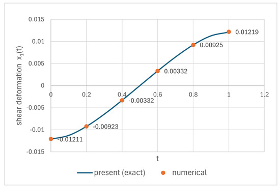
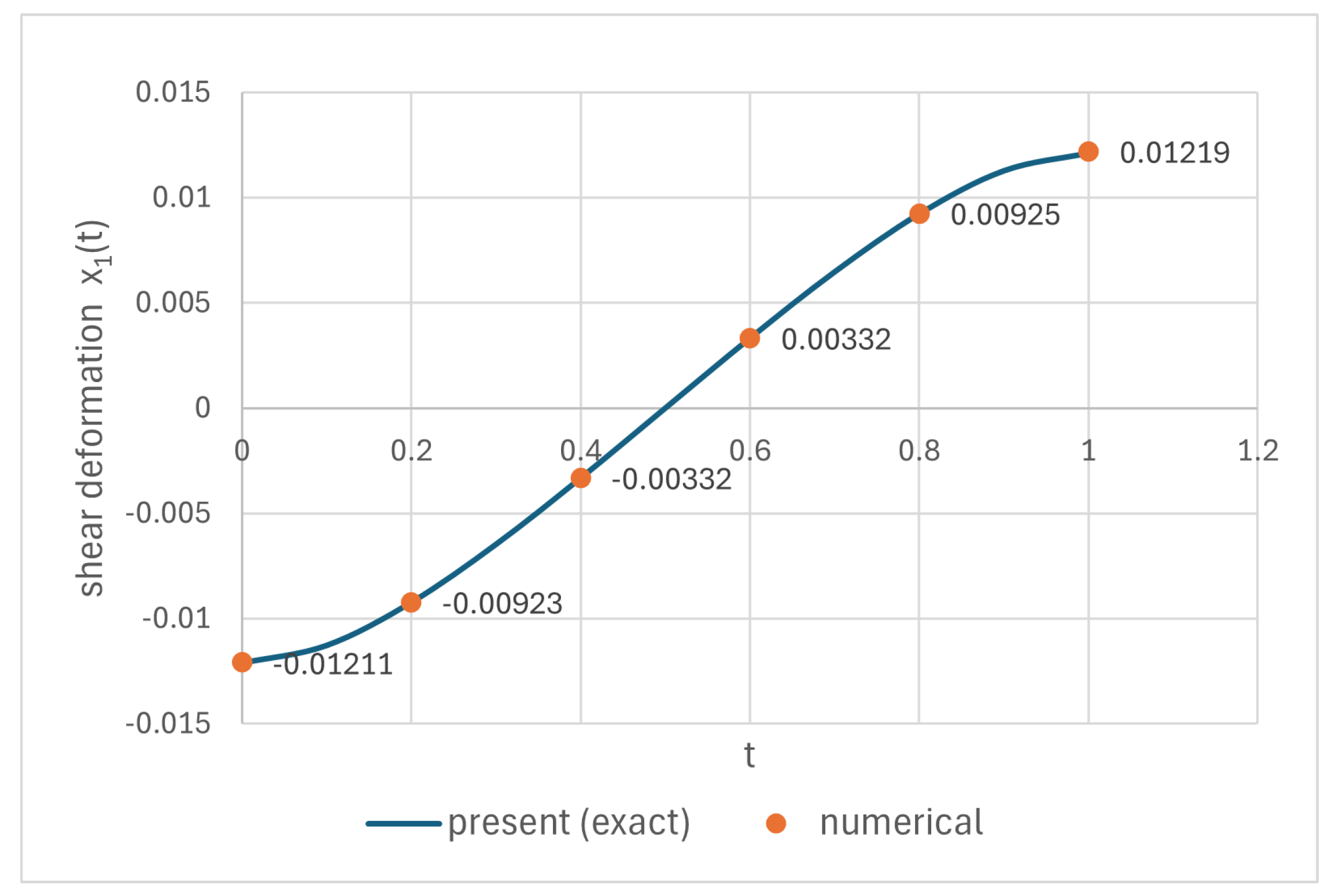
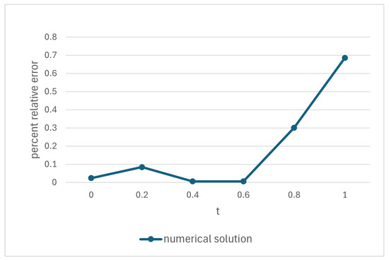
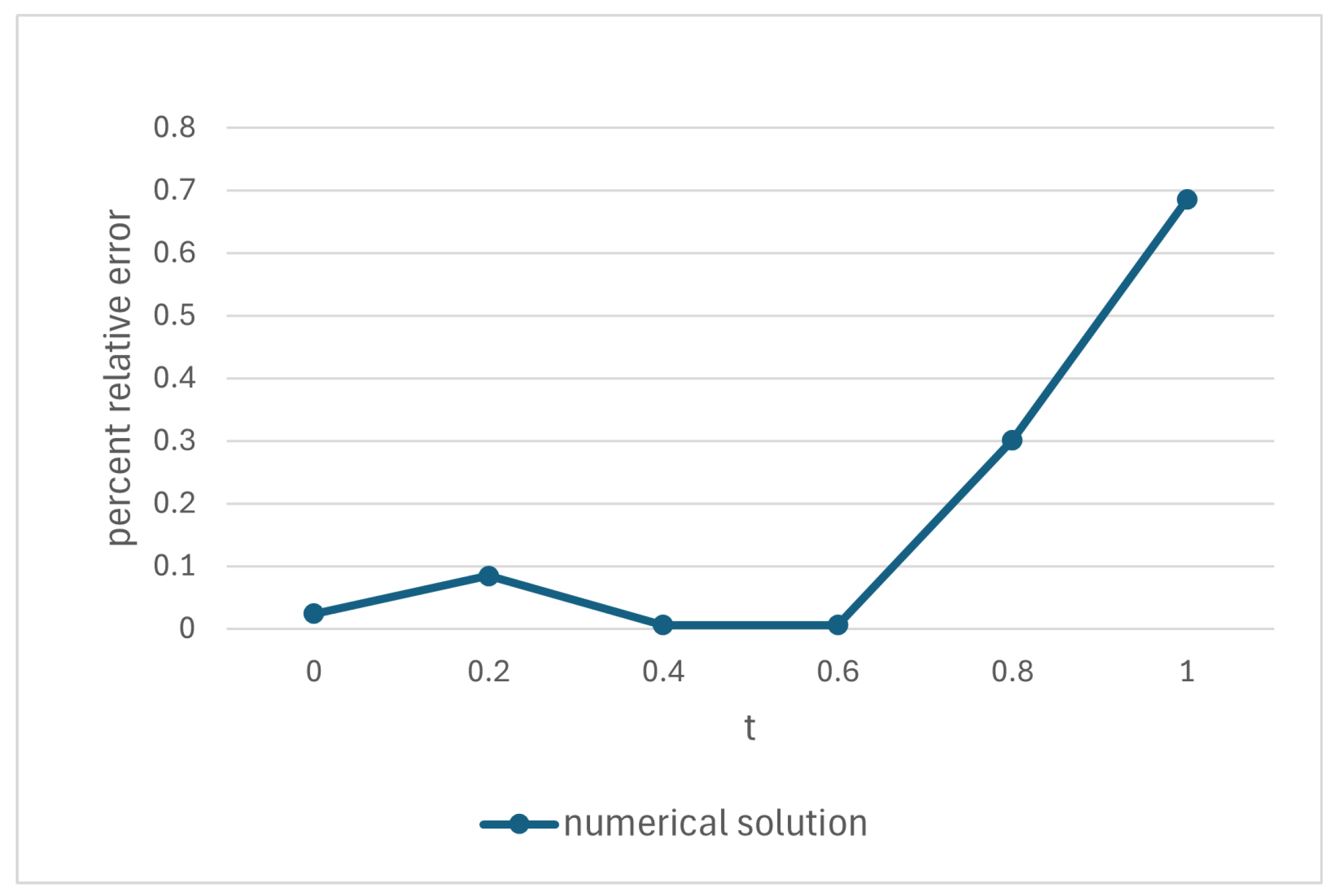
This problem with $k=5$ and $a=1$ was solved numerically in [32,33,34]. The numerical solution obtained by the weighted residuals method in [32] and the error compared to the present exact solution are depicted in Figure 1 and Figure 2, respectively.

Figure 1. Numerical solution (shear deformation) in [32] and the present exact solution.

Figure 2. Relative error rate of the numerical solution in [32] compared to the present exact solution.

Example DE.2 

Consider the system of two differential equations with variable coefficients,

$$\begin{array}{ccc}\hfill (t^2+1)x_1^{\prime }\left(t\right)-t{x}_1\left(t\right)+x_2\left(t\right)& =& 2t^4+4t^2-3,\hfill \\ \hfill (t^2+1)x_2^{\prime }\left(t\right)-x_1\left(t\right)-t{x}_2\left(t\right)& =& 5t,\hfill \end{array}$$

(45)

for $0\le t\le 1$, subject to the boundary conditions

$$\begin{array}{ccc}\hfill x_1\left(0\right)+x_2\left({\displaystyle \frac{1}{2}}\right)-2{\int }_{3/4}^{1}s{x}_1\left(s\right)ds& =& -{\displaystyle \frac{2183}{7680}},\hfill \\ \hfill x_1\left({\displaystyle \frac{1}{2}}\right)-4x_2\left(1\right)+{\int }_0^{1/4}\left(x_1\left(s\right)+2x_2\left(s\right)\right)ds& =& {\displaystyle \frac{4835}{3072}}.\hfill \end{array}$$

(46)

We take $n=2$, $\mathbb{X}=C[0,1]$ and put Equations (45) and (46) in the operator form as in Corollary 1, viz.

$${\mathcal{B}}_{d}x=\mathcal{A}x=f\left(t\right),\mathfrak{D}\left({\mathcal{B}}_d\right)=\{x\in {\mathbb{X}}_2^1:\theta \left(x\right)=c\},$$

where

$$\begin{array}{ccc}\hfill x\left(t\right)& =& {\left(\begin{array}{cc}{x}_1\left(t\right)& x_2\left(t\right)\end{array}\right)}^T,f\left(t\right)={\left(\begin{array}{cc}{\displaystyle \frac{2t^4+4t^2-3}{t^2+1}}& {\displaystyle \frac{5t}{t^2+1}}\end{array}\right)}^T,\hfill \\ \hfill \mathcal{A}x& =& x^{\prime }-A\left(t\right)x=x^{\prime }-\left[\begin{array}{cc}{\displaystyle \frac{t}{t^2+1}}& {\displaystyle \frac{-1}{t^2+1}}\\ {\displaystyle \frac{1}{t^2+1}}& {\displaystyle \frac{t}{t^2+1}}\end{array}\right]x,\hfill \\ \hfill \theta \left(x\right)& =& \left[\begin{array}{cc}1& 0\\ 0& 0\end{array}\right]x\left(0\right)+\left[\begin{array}{cc}0& 1\\ 1& 0\end{array}\right]x\left({\displaystyle \frac{1}{2}}\right)+\left[\begin{array}{cc}0& 0\\ 0& -4\end{array}\right]x\left(1\right)\hfill \\ & & +{\int }_0^{1/4}\left[\begin{array}{cc}0& 0\\ 1& 2\end{array}\right]x\left(s\right)ds+{\int }_{3/4}^1\left[\begin{array}{cc}-2s& 0\\ 0& 0\end{array}\right]x\left(s\right)ds,\hfill \\ \hfill c& =& {\left(\begin{array}{cc}-{\displaystyle \frac{2183}{7680}}& {\displaystyle \frac{4835}{3072}}\end{array}\right)}^T.\hfill \end{array}$$

Consider the complementary system as in Lemma 1, i.e.,

$$\widehat{\mathcal{A}}x=\mathcal{A}x=f\left(x\right),\mathfrak{D}\left(\widehat{\mathcal{A}}\right)=\left\{x\in {\mathbb{X}}_2^1:\widehat{\theta }\left(x\right)=x\left(0\right)=0\right\}.$$

It is known that the homogeneous system $\mathcal{A}x=0$ has the fundamental matrix

$$Z\left(t\right)=\left[\begin{array}{cc}1& -t\\ t& 1\end{array}\right],$$

which satisfies the equation $\widehat{\theta }\left(Z\right)=I_2$, see, for example, [35].

Then, from the proposed algorithm, we obtain

$$det\left(W_d\right)=-{\displaystyle \frac{1279}{384}}\ne 0,$$

which ensures that Equations (45) and (46) have a unique solution, which is

$$x_1\left(t\right)=t^3-2t,x_2\left(t\right)=t^2-1.$$

4.2. Integrodifferential Equations

Next, we solve a boundary value problem for a second-order FIDE and nonhomogeneous multipoint-integral conditions, and a boundary value problem for a system of two second-order FIDEs with nonhomogeneous mixed nonseparable conditions.

Example IDE.1  

In [36], a second order control problem for the dynamics of the rocket bank reduces to the second-order Fredholm integrodifferential equation

$${\chi }^{″}\left(t\right)+\nu {\chi }^{\prime }\left(t\right)+\mu {\int }_0^{T}K\left(s\right)\chi \left(s\right)ds=\mathfrak{f}\left(t\right),$$

(47)

with the boundary conditions

$$T\chi \left(0\right)+{\int }_0^T\chi \left(t\right)dt=0,{\chi }^{\prime }\left(T\right)=\phi ,$$

(48)

where $K\left(s\right),\mathfrak{f}\left(t\right)\in C[0,T]$, $\nu =1/T_0$, $\mu =\left(k_0{k}_1\right)/T_0$, $T_0,k_0,k_1,\phi$ are constants and $T>T_0$.

With the transformation $\chi \left(t\right)=x_1\left(t\right)$ and ${\chi }^{\prime }\left(t\right)=x_2\left(t\right)$ we can reduce Equations (47) and (48) to the following system of two first-order integrodifferential equations:

$$\begin{array}{ccc}\hfill x_1^{\prime }\left(t\right)-x_2\left(t\right)& =& 0,\hfill \\ \hfill x_2^{\prime }\left(t\right)+\nu x_2\left(t\right)+\mu {\int }_0^{T}K\left(s\right)x_1\left(s\right)ds& =& \mathfrak{f}\left(t\right),\hfill \end{array}$$

(49)

subject to the boundary conditions

$$T{x}_1\left(0\right)+{\int }_0^T{x}_1\left(s\right)ds=0,x_2\left(T\right)=\phi .$$

(50)

We set $\mathbb{X}=C[0,T]$, $n=2$ and $m=1$ and write Equations (49) and (50) in the operator form

$$\begin{array}{c}\hfill \mathcal{B}x=\mathcal{A}x-G\left(t\right)\eta \left(x\right),\mathfrak{D}\left(\mathcal{B}\right)=\left\{x\in {\mathbb{X}}_2^1:\theta \left(x\right)=c\right\},\end{array}$$

(51)

where

$$\begin{array}{ccc}\hfill x\left(t\right)& =& {\left(\begin{array}{cc}{x}_1\left(t\right)& x_2\left(t\right)\end{array}\right)}^T,f\left(t\right)={\left(\begin{array}{cc}0& \mathfrak{f}\left(t\right)\end{array}\right)}^T,\hfill \\ \hfill \mathcal{A}x& =& x^{\prime }-A\left(t\right)x=x^{\prime }-\left[\begin{array}{cc}0& 1\\ 0& -\nu \end{array}\right]x,\hfill \\ \hfill G\left(t\right)& =& \left[\begin{array}{c}0\\ -\mu \end{array}\right],\eta \left(x\right)=\left(\begin{array}{c}{\int }_0^T\left[\begin{array}{cc}K\left(s\right)& 0\end{array}\right]x\left(s\right)ds\end{array}\right),\hfill \\ \hfill \theta \left(x\right)& =& \left[\begin{array}{cc}T& 0\\ 0& 0\end{array}\right]x\left(0\right)+\left[\begin{array}{cc}0& 0\\ 0& 1\end{array}\right]x\left(T\right)+{\int }_0^T\left[\begin{array}{cc}1& 0\\ 0& 0\end{array}\right]x\left(s\right)ds,\hfill \\ \hfill c& =& {\left(\begin{array}{cc}0& \phi \end{array}\right)}^T.\hfill \end{array}$$

Let the complementary system in Lemma 1 be defined by

$$\widehat{\mathcal{A}}x=\mathcal{A}x=f\left(x\right),\mathfrak{D}\left(\widehat{\mathcal{A}}\right)=\left\{x\in {\mathbb{X}}_2^1:\widehat{\theta }\left(x\right)=x\left(0\right)=0\right\}.$$

The fundamental matrix of the homogeneous system $\mathcal{A}x=0$ is

$$Z\left(t\right)=\left[\begin{array}{cc}1& {\displaystyle \frac{1-e^{-\nu t}}{\nu }}\\ 0& e^{-\nu t}\end{array}\right],$$

which satisfies $\widehat{\theta }\left(Z\right)=I_2$.

Substituting into algorithm, we obtain that Equations (49) and (50) have a unique solution if and only if

$$det\left(W\right)=2T{e}^{-T\nu }\left(1-{\displaystyle \frac{\mu }{\nu }}{\int }_0^{T}K\left(s\right)[{\displaystyle \frac{T}{4}}-s-{\displaystyle \frac{1}{2T{\nu }^2}}+({\displaystyle \frac{1}{2T\nu }}-e^{-s\nu }+{\displaystyle \frac{1}{2}}){\displaystyle \frac{e^{T\nu }}{\nu }}]ds\right)\ne 0.$$

As a simple example, let $K\left(s\right)=1$, $\mathfrak{f}\left(t\right)=1$, $\nu =1/5$, $\phi =1$ and $T=10$. In this case the exact solution $x_1\left(t\right)$ of boundary value Equations (49) and (50) is

$$x_1\left(t\right)={\displaystyle \frac{e^{-\frac{t}{5}}\left(\left(\left(\left(125e^2+125\right)\mu -10\right)t-1250e^2\mu +30e^2+15\right)e^{\frac{t}{5}}+1250e^2\mu -40e^2\right)}{\left(125e^2-125\right)\mu -2}}.$$

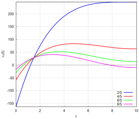
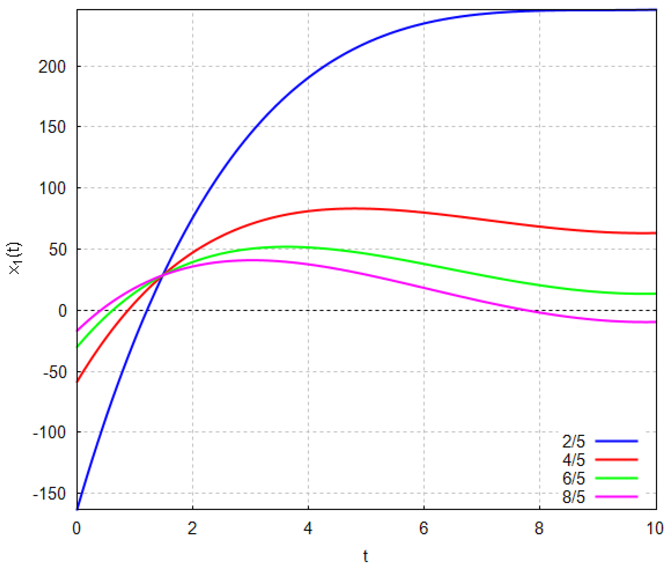
In the more complicated case for $K\left(s\right)=e^{-\nu t}/10$ and $\mathfrak{f}\left(t\right)=2t$, the solution is illustrated for different values of $\mu$ in Figure 3.

Figure 3. Exact solution of boundary value Equations (49) and (50) for different values of $\mu$.

Example IDE.2 

Consider the following system of two second-order linear Fredholm integrodifferential equations:

$$\begin{array}{ccc}\hfill u_1^{″}\left(t\right)+u_2^{\prime }\left(t\right)+{\int }_0^{1}2ts[u_1\left(s\right)-3u_2\left(s\right)]ds& =& 3t^2+{\displaystyle \frac{3t}{10}}+8,\hfill \\ \hfill u_1^{\prime }\left(t\right)+u_2^{″}\left(t\right)+{\int }_0^{1}3(2t+s^2)[u_1\left(s\right)-2u_2\left(s\right)]ds& =& 21t+{\displaystyle \frac{4}{5}},\hfill \end{array}$$

(52)

subject to the boundary conditions

$$\begin{array}{ccc}\hfill u_1\left(0\right)+u_1^{\prime }\left(0\right)& =& 1,\hfill \\ \hfill u_1\left(1\right)+u_1^{\prime }\left(1\right)& =& 10,\hfill \\ \hfill u_2\left(0\right)+u_2^{\prime }\left(0\right)& =& 1,\hfill \\ \hfill u_2\left(1\right)+u_2^{\prime }\left(1\right)& =& 7.\hfill \end{array}$$

(53)

This problem was solved numerically by the Tau method in [11].

To construct the exact solution we use the transformation $u_1\left(t\right)=x_1\left(t\right)$, $u_2\left(t\right)=x_2\left(t\right)$, $u_1^{\prime }\left(t\right)=x_3\left(t\right)$ and $u_2^{\prime }\left(t\right)=x_4\left(t\right)$ and write boundary value Equations (52) and (53) as a system of four first-order integrodifferential equations,

$$\begin{array}{ccc}\hfill x_1^{\prime }-x_3& =& 0,\hfill \\ \hfill x_2^{\prime }-x_4& =& 0,\hfill \\ \hfill x_3^{\prime }+x_4+2t{\int }_0^{1}s\left(x_1\left(s\right)-3x_2\left(s\right)\right)ds& =& 3t^2+{\displaystyle \frac{3t}{10}}+8,\hfill \\ \hfill x_4^{\prime }+x_3+6t{\int }_0^1\left(x_1\left(s\right)-2x_2\left(s\right)\right)ds+3{\int }_0^1{s}^2\left(x_1\left(s\right)-2x_2\left(s\right)\right)ds& =& 21t+{\displaystyle \frac{4}{5}},\hfill \end{array}$$

(54)

with the boundary conditions

$$\begin{array}{ccc}\hfill x_1\left(0\right)+x_3\left(0\right)& =& 1,\hfill \\ \hfill x_1\left(1\right)+x_3\left(1\right)& =& 10,\hfill \\ \hfill x_2\left(0\right)+x_4\left(0\right)& =& 1,\hfill \\ \hfill x_2\left(1\right)+x_4\left(1\right)& =& 7.\hfill \end{array}$$

(55)

In space $\mathbb{X}=C[0,1]$ and for $n=4$ and $m=3$, we write Equations (54) and (55) in the operator form

$$\mathcal{B}x=\mathcal{A}x-G\left(t\right)\eta \left(x\right),\mathfrak{D}\left(\mathcal{B}\right)=\left\{x\in {\mathbb{X}}_4^1:\theta \left(x\right)=c\right\},$$

where

$$\begin{array}{ccc}\hfill x\left(t\right)& =& {\left(\begin{array}{cccc}{x}_1\left(t\right)& x_2\left(t\right)& x_3\left(t\right)& x_4\left(t\right)\end{array}\right)}^T,f\left(t\right)={\left(\begin{array}{cccc}0& 0& 3t^2+{\displaystyle \frac{3t}{10}}+8& 21t+{\displaystyle \frac{4}{5}}\end{array}\right)}^T,\hfill \\ \hfill \mathcal{A}x& =& x^{\prime }-A\left(t\right)x=x^{\prime }-\left[\begin{array}{cccc}0& 0& 1& 0\\ 0& 0& 0& 1\\ 0& 0& 0& -1\\ 0& 0& -1& 0\end{array}\right]x,\hfill \\ \hfill G\left(t\right)& =& \left[\begin{array}{ccc}0& 0& 0\\ 0& 0& 0\\ 0& -2t& 0\\ -6t& 0& -3\end{array}\right],\eta \left(x\right)=\left(\begin{array}{c}{\int }_0^1\left[\begin{array}{cccc}1& -2& 0& 0\\ s& -3s& 0& 0\\ s^2& -2s^2& 0& 0\end{array}\right]x\left(s\right)ds\end{array}\right),\hfill \\ \hfill \theta \left(x\right)& =& \left[\begin{array}{cccc}1& 0& 1& 0\\ 0& 0& 0& 0\\ 0& 1& 0& 1\\ 0& 0& 0& 0\end{array}\right]x\left(0\right)+\left[\begin{array}{cccc}0& 0& 0& 0\\ 1& 0& 1& 0\\ 0& 0& 0& 0\\ 0& 1& 0& 1\end{array}\right]x\left(1\right),c=\left(\begin{array}{c}1\\ 10\\ 1\\ 7\end{array}\right).\hfill \end{array}$$

Let the complementary system in Lemma 1 be defined by

$$\widehat{\mathcal{A}}x=\mathcal{A}x=f\left(x\right),\mathfrak{D}\left(\widehat{\mathcal{A}}\right)=\left\{x\in {\mathbb{X}}_4^1:\widehat{\theta }\left(x\right)=x\left(0\right)=0\right\},$$

where, since the matrix A is constant, it is easy to construct a fundamental set of solutions of the homogeneous system $\mathcal{A}x=0$, namely

$$Z\left(t\right)=\left[\begin{array}{cccc}1& 0& sinh\left(t\right)& 1-cosh\left(t\right)\\ 0& 1& 1-cosh\left(t\right)& sinh\left(t\right)\\ 0& 0& cosh\left(t\right)& -sinh\left(t\right)\\ 0& 0& -sinh\left(t\right)& cosh\left(t\right)\end{array}\right],$$

which satisfies the equation $\widehat{\theta }\left(Z\right)=I_4$.

By substituting into the algorithm, we obtain the unique solution of Equations (54) and (55) as follows:

$$x\left(t\right)={\left(\begin{array}{cccc}3t^2+1& t^3+2t-1& 6t& 3t^2+2\end{array}\right)}^T.$$

5. Conclusions

Solvability criteria for general nonlocal boundary value problems for systems of linear ordinary integrodifferential equations of Fredholm type have been derived in a computationally convenient matrix form. A direct operator method for constructing their exact solution has also been presented. The method can be easily implemented in any computer algebra system. The main advantage is its ease of use and efficiency. Its disadvantage is the requirement of the fundamental matrix of the corresponding homogeneous differential system, which limits its application to cases where the matrix of coefficients is constant or is a matrix with variable coefficients of a special form.

The proposed method will be useful to many researchers as well as educational professionals in teaching advanced mathematics. Exact solutions are always necessary to validate numerical methods.

Although only integrodifferential equations are investigated here, Equations (6) and (7) are more general and describe various types of nonlocal boundary value problems. In particular, when the functionals ${\eta }_j$ are values of x at certain fixed points $\check{t}\in [a,b]$, then Equation (6) becomes a system of differential-boundary equations or loaded differential equations. Therefore, the solvability criteria and the solution method derived here can be extended to nonlocal boundary value problems for systems of linear ordinary loaded differential and loaded integrodifferential equations.

References

- Kiguradze, I.T. Boundary-value problems for systems of ordinary differential equations. J. Math. Sci. 1988, 43, 2259–2339. [Google Scholar] [CrossRef] [Scilit]
- Jerri, A.J. Introduction to Integral Equations with Applications, 2nd ed.; John Wiley & Sons: Hoboken, NJ, USA, 1999. [Google Scholar]
- Corduneanu, C. Integral Equations and Applications; Cambridge University Press: Cambridge, UK, 1991. [Google Scholar]
- Byszewski, L. Theorems about the existence and uniqueness of solutions of a semilinear evolution nonlocal Cauchy problem. J. Math. Anal. Appl. 1991, 162, 494–505. [Google Scholar] [CrossRef] [Scilit]
- Ntouyas, S.K. Chapter 6 Nonlocal Initial and Boundary Value Problems: A Survey. In Handbook of Differential Equations: Ordinary Differential Equations; Cañada, A., Drábek, P., Fonda, A., Eds.; North-Holland: Amsterdam, The Netherlands, 2006; pp. 461–557. [Google Scholar] [CrossRef] [Scilit]
- Štikonas, A. A Survey on stationary problems, Green’s functions and spectrum of Sturm–Liouville problem with nonlocal boundary conditions. Nonlinear Anal. Model. Control 2014, 19, 301–334. [Google Scholar] [CrossRef] [Scilit]
- McKibben, M. Discovering Evolution Equations with Applications: Volume 1-Deterministic Equations, 1st ed.; Chapman and Hall/CRC: Boca Raton, FL, USA, 2010; pp. 393–403. [Google Scholar] [CrossRef] [Scilit]
- Styś, K.; Styś, T. A higher-order finite difference method for solving a system of integro-differential equations. J. Comput. Appl. Math. 2000, 126, 33–46. [Google Scholar] [CrossRef] [Scilit]
- Zhao, J.; Corless, R.M. Compact finite difference method for integro-differential equations. Appl. Math. Comput. 2006, 177, 271–288. [Google Scholar] [CrossRef] [Scilit]
- Ghasemi, M.; Fardi, M.; Moradi, E. A Reproducing Kernel Method for Solving Systems of Integro-differential Equations with Nonlocal Boundary Conditions. Iran. J. Sci. Technol. Trans. Sci. 2021, 45, 1375–1382. [Google Scholar] [CrossRef] [Scilit]
- Pour-Mahmoud, J.; Rahimi-Ardabili, M.Y.; Shahmorad, S. Numerical solution of the system of Fredholm integro-differential equations by the Tau method. Appl. Math. Comput. 2005, 168, 465–478. [Google Scholar] [CrossRef] [Scilit]
- Vassiliev, N.; Parasidis, I.; Providas, E. Exact solution method for Fredholm integro-differential equations with multipoint and integral boundary conditions. Part 1. Extention method. Inf. Control Syst. 2018, 6, 14–23. [Google Scholar] [CrossRef] [Scilit]
- Tsilika, K.D. An exact solution method for Fredholm integro-differential equations. Inform.-Upravl. Sist. 2019, 4, 2–8. [Google Scholar] [CrossRef] [Scilit]
- Providas, E.; Parasidis, I.N. A Procedure for Factoring and Solving Nonlocal Boundary Value Problems for a Type of Linear Integro-Differential Equations. Algorithms 2021, 14, 346. [Google Scholar] [CrossRef] [Scilit]
- Providas, E. On the Exact Solution of Nonlocal Euler–Bernoulli Beam Equations via a Direct Approach for Volterra-Fredholm Integro-Differential Equations. AppliedMath 2022, 2, 269–283. [Google Scholar] [CrossRef] [Scilit]
- Samoilenko, A.M.; Boichuk, O.A.; Krivosheya, S.A. Boundary-Value problems for systems of integro-differential equations with Degenerate Kernel. Ukr. Math. J. 1996, 48, 1785–1789. [Google Scholar] [CrossRef] [Scilit]
- Boichuk, A.A.; Zhuravlev, V.F. Solvability Criterion for Integro-Differential Equations with Degenerate Kernel in Banach Spaces. Nonlinear Dyn. Syst. Theory 2018, 18, 331–341. [Google Scholar]
- Boichuk, A.A.; Zhuravlev, V.F. Solvability Criterion for Linear Boundary-Value Problems for Integrodifferential Fredholm Equations with Degenerate Kernels in Banach Spaces. Ukr. Math. J. 2021, 72, 1695–1714. [Google Scholar] [CrossRef] [Scilit]
- Aida-Zade, K.R.; Abdullayev, V.M. To the solution of integro-differential equations with nonlocal conditions. Turk. J. Math. 2022, 46, 177–188. [Google Scholar] [CrossRef] [Scilit]
- Baiburin, M.M.; Providas, E. Exact Solution to Systems of Linear First-Order Integro-Differential Equations with Multipoint and Integral Conditions. In Mathematical Analysis and Applications, Springer Optimization and Its Applications 154; Rassias, T.M., Pardalos, P.M., Eds.; Springer Nature: Cham, Switzerland, 2019; pp. 1–16. [Google Scholar] [CrossRef] [Scilit]
- Balachandran, K.; Kiruthika, S. Existence results for fractional integrodifferential equations with nonlocal condition via resolvent operators. Comput. Math. Appl. 2011, 62, 1350–1358. [Google Scholar] [CrossRef] [Scilit]
- Gupta, V.; Dabas, J. Existence results for a fractional integrodifferential equation with nonlocal boundary conditions and fractional impulsive conditions. Nonlinear Dyn. Syst. Theory 2015, 15, 370–382. [Google Scholar]
- Ahmad, B.; Alnahdi, M.; Ntouyas, S.K. Existence Results for a Differential Equation Involving the Right Caputo Fractional Derivative and Mixed Nonlinearities with Nonlocal Closed Boundary Conditions. Fractal Fract. 2023, 7, 129. [Google Scholar] [CrossRef] [Scilit]
- Moler, C.; Van Loan, C. Nineteen Dubious Ways to Compute the Exponential of a Matrix, Twenty-Five Years Later. SIAM Rev. 2003, 45, 3–49. [Google Scholar] [CrossRef] [Scilit]
- Krall, A.M. Differential-boundary operators. Trans. Amer. Math. Soc. 1971, 154, 429–458. [Google Scholar] [CrossRef]
- Nakhushev, A.M. Loaded equations and their applications. Differ. Uravn. 1983, 19, 86–94. (In Russian) [Google Scholar]
- Winkler, F. Symbolic computation in algebra, geometry, and differential equations. Inf. Comput. 2024, 301, 105200. [Google Scholar] [CrossRef] [Scilit]
- Mélard, G. A Symbolic Algorithm for Checking the Identifiability of a Time-Series Model. Information 2025, 16, 16. [Google Scholar] [CrossRef] [Scilit]
- Kokebaev, B.K.; Otelbaev, M.; Shynibekov, A.N. About Restrictions and Extensions of operators. Dokl. Akad. Nauk. SSSR 1983, 271, 1307–1310. (In Russian) [Google Scholar]
- Gusev, A.A.; Gerdt, V.P.; Hai, L.L.; Derbov, V.L.; Vinitsky, S.I.; Chuluunbaatar, O. Symbolic-Numeric Algorithms for Solving BVPs for a System of ODEs of the Second Order: Multichannel Scattering and Eigenvalue Problems. In Computer Algebra in Scientific Computing; CASC 2016. Lecture Notes in Computer Science; Gerdt, V., Koepf, W., Seiler, W., Vorozhtsov, E., Eds.; Springer: Cham, Switzerland, 2016; Volume 9890. [Google Scholar] [CrossRef] [Scilit]
- Na, T.Y. Computational Methods in Engineering Boundary Value Problems; Academic Press: New York, NY, USA, 1979. [Google Scholar]
- Haque, M.; Baluch, M.H.; Mohsen, M.F.N. Solution of multiple point, nonlinear boundary value problems by method of weighted residuals. Int. J. Comput. Math. 1986, 19, 69–84. [Google Scholar] [CrossRef] [Scilit]
- Liu, G.R.; Wu, T.Y. Multipoint boundary value problems by differential quadrature method. Math. Comput. Model. 2002, 35, 215–227. [Google Scholar] [CrossRef] [Scilit]
- Groza, G.; Pop, N. Approximate solution of multipoint boundary value problems for linear differential equations by polynomial functions. J. Differ. Equ. Appl. 2008, 14, 1289–1309. [Google Scholar] [CrossRef] [Scilit]
- Shirley, K.L.; Klima, V.W. Linear ODE Systems Having a Fundamental Matrix of the Form f(Mt). CODEE J. 2024, 18, 2. [Google Scholar] [CrossRef] [Scilit]
- Yuldashev, T.K. Nonlocal Boundary Value Problem for a Nonlinear Fredholm Integro-Differential Equation with Degenerate Kernel. Differ. Equ. 2018, 54, 1646–1653. [Google Scholar] [CrossRef] [Scilit]
Disclaimer/Publisher’s Note: The statements, opinions and data contained in all publications are solely those of the individual author(s) and contributor(s) and not of MDPI and/or the editor(s). MDPI and/or the editor(s) disclaim responsibility for any injury to people or property resulting from any ideas, methods, instructions or products referred to in the content. |
© 2026 by the authors. Licensee MDPI, Basel, Switzerland. This article is an open access article distributed under the terms and conditions of the Creative Commons Attribution (CC BY) license.