Improved Nonparallel Support Vector Machine for Pattern Classification

Abstract

In this paper, we propose a new nonparallel support vector machine for binary classification problems and name it the improved nonparallel support vector machine (IMNSVM). The IMNSVM uses a one-sided $\epsilon$-band and minimizes $\epsilon$ to achieve a better fitting effect for the same class of training points. By introducing a new variable, $\rho$, the IMNSVM keeps one class of training points at a certain distance from the hyperplane corresponding to another class of training points, keeping them as far away as possible so as to better adapt to the training points and better describe the difference in data distribution between different categories. The IMNSVM can degenerate into the standard support vector machine (SVM) under certain conditions and is applicable to a wider range of data types. Finally, numerical experiments also explain the effectiveness of the method.

1. Introduction

Support vector machines (SVMs) [1,2,3] are some of the most important tools in machine learning. They use statistical and optimization methods to solve machine learning problems and offer advantages for dealing with small-sample machine learning problems. Support vector machines have achieved great success in many fields, such as image segmentation, handwriting recognition, face recognition, text classification, and strip-steel surface defect classification [4,5,6,7,8,9,10,11,12]. However, in the era of big data, compared to the flourishing development of deep learning and reinforcement learning, research on SVMs has fallen into a slump. Due to the advantages of SVMs, such as simple and clear principles, a solid statistical learning theory foundation, and outstanding practical computational effects, research on theories, models, and algorithms pertaining to SVMs has been ongoing.

Recently, nonparallel support vector machines have attracted a great deal of research attention. Mangasarian [13] proposed the earliest nonparallel classifier and named it the generalized eigenvalue proximal support vector machine (GEPSVM). By solving two related generalized eigenvalue problems, the GEPSVM determines two nonparallel hyperplanes. Jayadeva [14] proposed twin support vector machine (TWSVM). The TWSVM is designed to generate a pair of nonparallel hyperplanes so that each class of points is as close to its corresponding hyperplane as possible and far away from the hyperplane corresponding to another class of points. TWSVMs [14,15,16] solve two small quadratic programming problems (QPPs) instead of the large quadratic programming problem (QPP) addressed by a traditional support vector machine.Their calculation efficiency is faster, and the effect is more significant. Shao [17] proposed TBSVM, which introduced regularization terms on the basis of TWSVM to reduce structural risk. TBSVM can classify multidimensional complex data better than TWSVM. Tian [18] proposed the nonparallel support vector machine (NPSVM). By adding an $\epsilon$-band, the NPSVM posed two new small quadratic programming problems, and, like SVMs, it has various advantages, such as sparsity, direct application of the kernel trick in nonlinear cases, and a lack of a requirement for matrix inversion in the calculation process. The study of nonparallel support vector machines has become an important direction of classification research [19,20,21,22,23,24,25,26].

Let us compare support vector machines with nonparallel support vector machines. SVMs are more theoretically mature, but their decision boundaries are relatively rigid, and they demand higher computational complexity for large-scale data. Nonparallel support vector machines can be decomposed into sub-problems for computation, making them more suitable for large-scale data and more robust to noise. They are also suitable for nonparallel data and can be extended to multi-classification problems, making them more suitable for complex distributions and multi-modal problems. In practice, it may be necessary to choose a method through cross-validation verification based on the complexity of the problem, data size, and interpretability requirements. The NSVM proposed by Shao [27] introduced a new soft-interval $\epsilon$-insensitive loss function for classification problems and fitted the dense regions of each class of training points by minimizing the one-sided $\epsilon$-band. The NSVM is a nonparallel support vector machine model that can degenerate into the standard SVM under certain conditions. It can achieve conversion between parallel and nonparallel algorithms and be used for a wider range of data classification.

In this paper, we further investigate nonparallel support vector machines, which can degenerate into SVMs, and propose the IMNSVM. We introduce a new variable that is not used in the NSVM: $\rho$. By adjusting this variable, we can ensure each class of training points is as far as possible from the hyperplane corresponding to another class of training points to improve the separation of training points so that the model has a better classification effect.

This paper is organized as follows. The C-SVM, TBSVM, NPSVM, and NSVM are briefly reviewed in Section 2. We introduce the improved nonparallel support vector machine (IMNSVM) in Section 3. The experimental results are presented in Section 4. In Section 5, the conclusions are given.

2. Background

In this section, we briefly introduce some support vector classifiers. Consider the binary classification problem with the following training set:

$$T=\{(x_1,+1),(x_2,+1),\cdots ,(x_p,+1),(x_{p+1},-1),(x_{p+2},-1),\cdots ,(x_{p+q},-1)\},$$

(1)

where $x_i\in R^n,i=1,2,\cdots ,p+q$ are inputs, and $+1,-1$ are outputs.

2.1. C-SVM

In the linear case, C-SVM seeks the separation hyperplane

$$(\omega ·x)+b=0$$

via a QPP as follows:

$$\begin{array}{c}{\displaystyle \underset{\omega ,b,\xi }{\min }\frac{1}{2}{\Vert \omega \Vert }^2+C\sum _{i=1}^{p+q}{\xi }_i}\hfill \\ \mathrm{s.t.}{y}_i((\omega ·x_i)+b)\ge 1-{\xi }_i,i=1,2,\cdots ,p+q,\hfill \\ {\xi }_i\ge 0,i=1,2,\cdots ,p+q,\hfill \end{array}$$

(2)

where $\omega \in R^n$, $y_i\in \{+1,-1\},i=1,2,\cdots ,p+q$, $b\in R$, $C>0$ is a parameter, and ${\xi }_i,$$i=1,2,\cdots ,p+q$ is the slack variable. C-SVM has sparsity and solves its dual problem to implement classification. The kernel trick can be directly applied in the nonlinear case because only the inner products exist in the dual problem.

2.2. TBSVM

Linear TBSVM seeks a pair of nonparallel hyperplanes

$$({\omega }_1·x)+b_1=0\mathrm{and}({\omega }_2·x)+b_2=0$$

(3)

by solving two QPPs

$$\begin{array}{c}{\displaystyle \underset{{\omega }_1,b_1,{\xi }_2}{\min }\frac{1}{2}{c}_1(\Vert {\omega }_1{\Vert }^2+b_1^2)+\frac{1}{2}{(A{\omega }_1+e_1{b}_1)}^{\mathrm{T}}(A{\omega }_1+e_1{b}_1)+c_2{e}_2^{\mathrm{T}}{\xi }_2}\hfill \\ \mathrm{s.t.}-(B{\omega }_1+e_2{b}_1)+{\xi }_2\ge e_2,{\xi }_2\ge 0,\hfill \end{array}$$

(4)

and

$$\begin{array}{c}{\displaystyle \underset{{\omega }_2,b_2,{\xi }_1}{\min }\frac{1}{2}{c}_3(\Vert {\omega }_2{\Vert }^2+b_2^2)+\frac{1}{2}{(B{\omega }_2+e_2{b}_2)}^{\mathrm{T}}(B{\omega }_2+e_2{b}_2)+c_4{e}_1^{\mathrm{T}}{\xi }_1}\hfill \\ \mathrm{s.t.}(A{\omega }_2+e_1{b}_2)+{\xi }_1\ge e_1,{\xi }_1\ge 0,\hfill \end{array}$$

(5)

where ${\omega }_k\in R^n$, $b_k\in R,k=1,2$. $c_i>0,i=1,2,3,4$ are parameters, $e_1={(1,1,\cdots ,1)}^T\in R^p$, $e_2={(1,1,\cdots ,1)}^T\in R^q$, $A={(x_1,x_2,\cdots ,x_p)}^{\mathrm{T}}\in R^{p\times n}$, $B={(x_{p+1},x_{p+2},\cdots ,x_{p+q})}^{\mathrm{T}}\in R^{q\times n}$, and ${\xi }_1\in R^p$ and ${\xi }_2\in R^q$ are slack variables. TBSVM has difficultly solving the problem posed by an inverse matrix when there are many data. In the nonlinear case, two extra kernel-generated surfaces need be given to replace hyperplanes. Even with linear kernels, the nonlinear classifiers cannot degenerate into linear classifiers.

2.3. NPSVM

The linear NPSVM, given the following two QPPs, seeks two nonparallel hyperplanes (3):

$$\begin{array}{c}{\displaystyle \underset{{\omega }_1,b_1,{\xi }_1,{\xi }_1^{*},{\eta }_2}{\min }\frac{1}{2}{\Vert {\omega }_1\Vert }^2+C_1\sum _{i=1}^p({\xi }_{1i}+{\xi }_{1i}^{*})+C_2\sum _{j=p+1}^{p+q}{\eta }_{2j}}\hfill \\ \mathrm{s.t.}({\omega }_1·x_i)+b_1\le \epsilon +{\xi }_{1i},i=1,2,\cdots ,p,\hfill \\ -({\omega }_1·x_i)-b_1\le \epsilon +{\xi }_{1i}^{*},i=1,2,\cdots ,p,\hfill \\ ({\omega }_1·x_j)+b_1\le -1+{\eta }_{2j},j=p+1,p+2,\cdots ,p+q,\hfill \\ {\xi }_{1i},{\xi }_{1i}^{*}\ge 0,i=1,2,\cdots ,p,\hfill \\ {\eta }_{2j}\ge 0,j=p+1,p+2,\cdots ,p+q,\hfill \end{array}$$

(6)

and

$$\begin{array}{c}{\displaystyle \underset{{\omega }_2,b_2,{\xi }_2,{\xi }_2^{*},{\eta }_1}{\min }\frac{1}{2}{\Vert {\omega }_2\Vert }^2+C_3\sum _{i=p+1}^{p+q}({\xi }_{2i}+{\xi }_{2i}^{*})+C_4\sum _{j=1}^p{\eta }_{1j}}\hfill \\ \mathrm{s.t.}({\omega }_2·x_i)+b_2\le \epsilon +{\xi }_{2i},i=p+1,p+2,\cdots ,p+q,\hfill \\ -({\omega }_2·x_i)-b_2\le \epsilon +{\xi }_{2i}^{*},i=p+1,p+2,\cdots ,p+q,\hfill \\ ({\omega }_2·x_j)+b_2\ge 1-{\eta }_{1j},j=1,2,\cdots ,p,\hfill \\ {\xi }_{2i},{\xi }_{2i}^{*}\ge 0,i=p+1,p+2,\cdots ,p+q,\hfill \\ {\eta }_{1j}\ge 0,j=1,2,\cdots ,p,\hfill \end{array}$$

(7)

where $x_i,i=1,2,\cdots ,p$ are positive points; $x_j,j=p+1,p+2,\cdots ,p+q$ are negative points; $C_i>0,i=1,2,3,4$ are parameters; and ${\xi }_1={({\xi }_{11},{\xi }_{12},\cdots ,{\xi }_{1p})}^{\mathrm{T}}$, ${\xi }_1^{*}=({\xi }_{11}^{*},{\xi }_{12}^{*},\cdots$,${{\xi }_{1p}^{*})}^{\mathrm{T}}$, ${\xi }_2=({\xi }_{2,p+1},{\xi }_{2,p+2},\cdots ,$${{\xi }_{2,p+q})}^{\mathrm{T}}$, ${\xi }_2^{*}={({\xi }_{2,p+1}^{*},{\xi }_{2,p+2}^{*},\cdots ,{\xi }_{2,p+q}^{*})}^{\mathrm{T}}$, ${\eta }_1={({\eta }_{11},{\eta }_{12},\cdots ,{\eta }_{1p})}^{\mathrm{T}}$, and ${\eta }_2={({\eta }_{2,p+1},{\eta }_{2,p+2},\cdots ,{\eta }_{2,p+q})}^{\mathrm{T}}$ are slack variables. Taking the positive points as an example, this model requires as many positive points as possible between the hyperplanes $({\omega }_1·x)+b_1=\epsilon$ and $({\omega }_1·x)+b_1=-\epsilon$.

2.4. NSVM

The NSVM introduces a new soft-interval $\epsilon$-insensitive loss function for classification problems:

$$l(x,y,g_k)=\left\{\begin{array}{cc}1-y(w_k^{\mathrm{T}}x+b_k),\hfill & y(w_k^{\mathrm{T}}x+b_k)\le 1,\hfill \\ 0,\hfill & 1\le y(w_k^{\mathrm{T}}x+b_k)\le 1+\epsilon ,\hfill \\ y(w_k^{\mathrm{T}}x+b_k)-(1+\epsilon ),\hfill & \mathrm{else}.\hfill \end{array}\right.$$

where $k=1,2,$$x\in R^n$ are inputs, and $y\in \{+1,-1\}$ are outputs.

In the linear case, the NSVM solves two primal problems:

$$\begin{array}{c}{\displaystyle \underset{{\omega }_1,b_1,{\epsilon }_1,{\xi }_1^{(\ast )},{\eta }_2}{\min }\frac{1}{2}{\Vert {\omega }_1\Vert }^2+\gamma {\epsilon }_1+C_1\sum _{i=1}^p({\xi }_{1i}+{\xi }_{1i}^{*})+C_2\sum _{j=p+1}^{p+q}{\eta }_{2j}}\hfill \\ \mathrm{s.t.}1-{\xi }_{1i}^{*}\le ({\omega }_1·x_i)+b_1\le 1+{\epsilon }_1+{\xi }_{1i},i=1,2,\cdots ,p,\hfill \\ ({\omega }_1·x_j)+b_1\le -1+{\eta }_{2j},j=p+1,p+2,\cdots ,p+q,\hfill \\ {\xi }_{1i},{\xi }_{1i}^{*}\ge 0,i=1,2,\cdots ,p,\hfill \\ {\eta }_{2j}\ge 0,j=p+1,p+2,\cdots ,p+q,\hfill \\ {\epsilon }_1\ge 0,\hfill \end{array}$$

and

$$\begin{array}{c}{\displaystyle \underset{{\omega }_2,b_2,{\epsilon }_2,{\xi }_2^{(\ast )},{\eta }_1}{\min }\frac{1}{2}{\Vert {\omega }_2\Vert }^2+\gamma {\epsilon }_2+C_1\sum _{i=1}^p{\eta }_{1i}+C_2\sum _{j=p+1}^{p+q}({\xi }_{2j}+{\xi }_{2j}^{*})}\hfill \\ \mathrm{s.t.}({\omega }_2·x_i)+b_2\ge 1-{\eta }_{1i},i=1,2,\cdots ,p,\hfill \\ -1-{\epsilon }_2-{\xi }_{2j}^{*}\le ({\omega }_2·x_j)+b_2\le -1+{\xi }_{2j},j=p+1,p+2,\cdots ,p+q,\hfill \\ {\eta }_{1i}\ge 0,i=1,2,\cdots ,p,\hfill \\ {\xi }_{2j},{\xi }_{2j}^{*}\ge 0,j=p+1,p+2,\cdots ,p+q,\hfill \\ {\epsilon }_2\ge 0,\hfill \end{array}$$

where  $C_i>0,i=1,2$ are the parameters. ${\xi }_1^{(\ast )}={({\xi }_1^{\mathrm{T}},{\xi }_1^{*\mathrm{T}})}^{\mathrm{T}}={({\xi }_{11},\cdots ,{\xi }_{1p},{\xi }_{11}^{*},\cdots ,{\xi }_{1p}^{*})}^{\mathrm{T}}$, ${\xi }_2^{(\ast )}={({\xi }_2^{\mathrm{T}},{\xi }_2^{*\mathrm{T}})}^{\mathrm{T}}=$ ${({\xi }_{2,p+1},\cdots ,{\xi }_{2,p+q},{\xi }_{2,p+1}^{*},\cdots ,{\xi }_{2,p+q}^{*})}^{\mathrm{T}}$, ${\eta }_1={({\eta }_{11},{\eta }_{12},\cdots ,{\eta }_{1p})}^{\mathrm{T}}$ and ${\eta }_2={({\eta }_{2,p+1},{\eta }_{2,p+2}\cdots ,{\eta }_{2,p+q})}^{\mathrm{T}}$ are slack variables.

For the positive points, the margin between the hyperplanes $({\omega }_1·x)+b_1=1$ and $({\omega }_1·x)+b_1=-1$ can be expressed as ${\displaystyle \frac{2}{\Vert {\omega }_1\Vert }}$. And ${\displaystyle \frac{{\epsilon }_1}{\Vert {\omega }_1\Vert }}$ is defined as the width of the one-sided $\epsilon$-band between the hyperplanes $({\omega }_1·x)+b_1=1$ and $({\omega }_1·x)+b_1=1+{\epsilon }_1$. By minimizing $\Vert {\omega }_1\Vert$, the negative points will be as far away as possible from the hyperplane corresponding to the positive points. Moreover, minimizing ${\epsilon }_1$ can reveal a one-sided $\epsilon$-band that is a better fit for the dense regions of the positive points.

3. IMNSVM

In this section, a new improved nonparallel support vector machine (IMNSVM) is proposed for binary classification with the training set (1).

3.1. Linear IMNSVM

3.1.1. The Original Problems

We look for a pair of nonparallel hyperplanes

$$({\omega }_1·x)+b_1=1\mathrm{and}({\omega }_2·x)+b_2=-1$$

(8)

by solving two QPPs,

$$\begin{array}{c}{\displaystyle \underset{{\omega }_1,b_1,{\epsilon }_1,{\xi }_1^{(\ast )},{\eta }_2,{\rho }_2}{\min }\frac{1}{2}(\Vert {\omega }_1{\Vert }^2+b_1^2)+r_1{\epsilon }_1+C_1\sum _{i=1}^p({\xi }_{1i}+{\xi }_{1i}^{*})-r_2{\rho }_2+C_2\sum _{j=p+1}^{p+q}{\eta }_{2j}}\hfill \\ \mathrm{s.t.}({\omega }_1·x_i)+b_1\le 1+{\epsilon }_1+{\xi }_{1i},i=1,2,\cdots ,p,\hfill \\ -({\omega }_1·x_i)-b_1\le -1+{\xi }_{1i}^{*},i=1,2,\cdots ,p,\hfill \\ ({\omega }_1·x_j)+b_1\le -{\rho }_2+{\eta }_{2j},j=p+1,p+2,\cdots ,p+q,\hfill \\ {\xi }_{1i}\ge 0,{\xi }_{1i}^{*}\ge 0,i=1,2,\cdots ,p,\hfill \\ {\eta }_{2j}\ge 0,j=p+1,p+2,\cdots ,p+q,\hfill \\ {\epsilon }_1\ge 0,{\rho }_2\ge 0,\hfill \end{array}$$

(9)

and

$$\begin{array}{c}{\displaystyle \underset{{\omega }_2,b_2,{\epsilon }_2,{\xi }_2^{(\ast )},{\eta }_1,{\rho }_1}{\min }\frac{1}{2}(\Vert {\omega }_2{\Vert }^2+b_2^2)+r_3{\epsilon }_2+C_3\sum _{j=p+1}^{p+q}({\xi }_{2j}+{\xi }_{2j}^{*})-r_4{\rho }_1+C_4\sum _{i=1}^p{\eta }_{1i}}\hfill \\ \mathrm{s.t.}-({\omega }_2·x_j)-b_2\le 1+{\epsilon }_2+{\xi }_{2j},j=p+1,p+2,\cdots ,p+q,\hfill \\ ({\omega }_2·x_j)+b_2\le -1+{\xi }_{2j}^{*},j=p+1,p+2,\cdots ,p+q,\hfill \\ -({\omega }_2·x_i)-b_2\le -{\rho }_1+{\eta }_{1i},i=1,2,\cdots ,p,\hfill \\ {\xi }_{2j}\ge 0,{\xi }_{2j}^{*}\ge 0,j=p+1,p+2,\cdots ,p+q,\hfill \\ {\eta }_{1i}\ge 0,i=1,2,\cdots ,p,\hfill \\ {\epsilon }_2\ge 0,{\rho }_1\ge 0,\hfill \end{array}$$

(10)

where $C_i>0$ and $r_i>0,i=1,2,3,4$ are parameters, and $x_i,i=1,2,\cdots ,p$ are positive points. $x_j,j=p+1,p+2,\cdots ,p+q$ are negative points, and ${\eta }_1={({\eta }_{11},{\eta }_{12},\cdots ,{\eta }_{1p})}^{\mathrm{T}}$, ${\eta }_2={({\eta }_{2,p+1},{\eta }_{2,p+2},\cdots ,{\eta }_{2,p+q})}^{\mathrm{T}}$, ${\xi }_1^{(\ast )}={({\xi }_1^{\mathrm{T}},{\xi }_1^{*\mathrm{T}})}^{\mathrm{T}}={({\xi }_{11},\cdots ,{\xi }_{1p},{\xi }_{11}^{*},\cdots ,{\xi }_{1p}^{*})}^{\mathrm{T}}$ and ${\xi }_2^{(\ast )}={({\xi }_2^{\mathrm{T}},{\xi }_2^{*\mathrm{T}})}^{\mathrm{T}}=$ ${({\xi }_{2,p+1},\cdots ,{\xi }_{2,p+q},{\xi }_{2,p+1}^{*},\cdots ,{\xi }_{2,p+q}^{*})}^{\mathrm{T}}$ are slack variables.

As with TBSVM, by introducing the transformation from $R^n$ to $R^{n+1}$, ${\displaystyle \frac{1+\rho }{\sqrt{\Vert {\omega }_1{\Vert }^2+b_1^2}}}$ is defined as the margin between the proximal hyperplane $({\omega }_1·x)+b_1=[{\omega }_1^T,b_1]{[x^T,1]}^T=1$ and the bounding hyperplane $({\omega }_1·x)+b_1=[{\omega }_1^T,b_1]{[x^T,1]}^T=-\rho$.

For problems (9) and (10), there are five parts in the objective function. The regularization term, serving as the first part, can ensure that structural risk is minimized. The second part minimizes $\epsilon$ to achieve a better fitting effect for the same class of training points. The third and fifth parts minimize the loss as much as possible. The first and fourth parts ensure that each class of training points remains a certain distance from the hyperplane corresponding to another class of training points, ensuring this distance is as large as possible. When $r_1=r_2=0,{\rho }_2=1,C_1=C_2$, problem (9) can degenerate into the standard SVM. When $r_3=r_4=0,{\rho }_1=1,C_3=C_4$, problem (10) can degenerate into the standard SVM too.

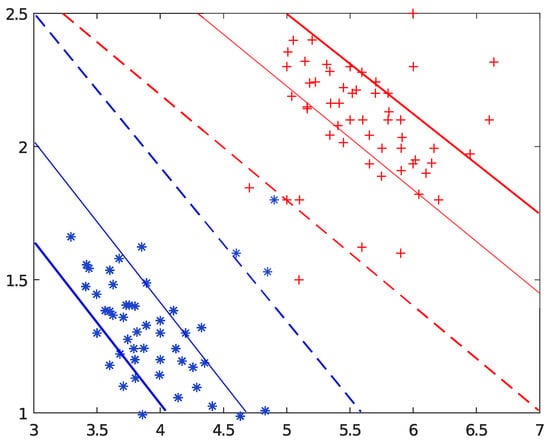
In geometry, we consider problem (9) in terms of $R^2$ (Figure 1). Firstly, we hope that as many and as dense positive points “+” as possible fall into the one-sided $\epsilon$-band between the hyperplanes $({\omega }_1·x)+b_1=1$ (red thin solid line) and $({\omega }_1·x)+b_1=1+{\epsilon }_1$ (red solid line), and $\epsilon$ is made as small as possible to achieve a better fitting effect. Secondly, we hope the negative points “∗” are below the hyperplane $({\omega }_1·x)+b_1=-{\rho }_2$ (red dotted line). The distance between the two is made as large as possible by maximizing ${\rho }_2$. Likewise, problem (10) can be represented by three blue lines.

Figure 1. Geometrical illustration of IMNSVM in $R^2$.

3.1.2. The Dual Problems

To solve problems (9) and (10), we should derive their dual problems. The Lagrangian function of problem (9) is given as follows:

$$\begin{array}{c}L({\omega }_1,b_1,{\epsilon }_1,{\xi }_1^{*},{\xi }_1,{\rho }_2,{\eta }_2,{\alpha }_1^{*},{\alpha }_1,{\beta }_2,{\lambda }_1^{*},{\lambda }_1,{\gamma }_2,{\theta }_1,{\theta }_2)\hfill \\ {\displaystyle =\frac{1}{2}(\Vert {\omega }_1{\Vert }^2+b_1^2)+r_1{\epsilon }_1+C_1{\displaystyle \sum _{i=1}^p}({\xi }_{1i}^{*}+{\xi }_{1i})-r_2{\rho }_2+C_2\sum _{j=p+1}^{p+q}{\eta }_{2j}}\hfill \\ +{\displaystyle \sum _{i=1}^p}{\alpha }_{1i}^{*}(({\omega }_1·x_i)+b_1-1-{\epsilon }_1-{\xi }_{1i}^{*})+{\displaystyle \sum _{i=1}^p}{\alpha }_{1i}(-({\omega }_1·x_i)-b_1+1-{\xi }_{1i})\hfill \\ +{\displaystyle \sum _{j=p+1}^{p+q}}{\beta }_{2j}(({\omega }_1·x_j)+b_1+{\rho }_2-{\eta }_{2j})-{\displaystyle \sum _{i=1}^p}{\lambda }_{1i}^{*}{\xi }_{1i}^{*}-{\displaystyle \sum _{i=1}^p}{\lambda }_{1i}{\xi }_{1i}\hfill \\ -{\displaystyle \sum _{j=p+1}^{p+q}}{\gamma }_{2j}{\eta }_{2j}-{\theta }_1{\epsilon }_1-{\theta }_2{\rho }_2,\hfill \end{array}$$

(11)

where ${\alpha }_1^{*}={({\alpha }_{11}^{*},{\alpha }_{12}^{*},\cdots ,{\alpha }_{1p}^{*})}^{\mathrm{T}}$, ${\alpha }_1={({\alpha }_{11},{\alpha }_{12},\cdots ,{\alpha }_{1p})}^{\mathrm{T}}$, ${\beta }_2={({\beta }_{2,p+1},{\beta }_{2,p+2},\cdots ,{\beta }_{2,p+q})}^{\mathrm{T}}$, ${\lambda }_1^{*}={({\lambda }_{11}^{*},{\lambda }_{12}^{*},\cdots ,{\lambda }_{1p}^{*})}^{\mathrm{T}}$, ${\lambda }_1={({\lambda }_{11},{\lambda }_{12},\cdots ,{\lambda }_{1p})}^{\mathrm{T}}$, ${\gamma }_2={({\gamma }_{2,p+1},{\gamma }_{2,p+2},\cdots ,{\gamma }_{2,p+q})}^{\mathrm{T}}$, ${\theta }_1\in R$, and ${\theta }_2\in R$ are the Lagrange multipliers. Applying the Karush–Kuhn–Tucker (KKT) conditions [28] leaves us with

$$\begin{array}{cc}\hfill {\nabla }_{{\omega }_1}L& ={\omega }_1+\sum _{i=1}^p{\alpha }_{1i}^{*}{x}_i-\sum _{i=1}^p{\alpha }_{1i}{x}_i+\sum _{j=p+1}^{p+q}{\beta }_{2j}{x}_j=0,\hfill \end{array}$$

(12)

$$\begin{array}{cc}\hfill {\nabla }_{b_1}L& =b_1+\sum _{i=1}^p{\alpha }_{1i}^{*}-\sum _{i=1}^p{\alpha }_{1i}+\sum _{j=p+1}^{p+q}{\beta }_{2j}=0,\hfill \end{array}$$

(13)

$$\begin{array}{cc}\hfill {\nabla }_{{\epsilon }_1}L& =r_1-\sum _{i=1}^p{\alpha }_{1i}^{*}-{\theta }_1=0,\hfill \end{array}$$

(14)

$$\begin{array}{cc}\hfill {\nabla }_{{\xi }_1^{*}}L& =C_1{e}_1-{\alpha }_1^{*}-{\lambda }_1^{*}=0,\hfill \end{array}$$

(15)

$$\begin{array}{cc}\hfill {\nabla }_{{\xi }_1}L& =C_1{e}_1-{\alpha }_1-{\lambda }_1=0,\hfill \end{array}$$

(16)

$$\begin{array}{cc}\hfill {\nabla }_{{\rho }_2}L& =-r_2+\sum _{j=p+1}^{p+q}{\beta }_{2j}-{\theta }_2=0,\hfill \end{array}$$

(17)

$$\begin{array}{cc}\hfill {\nabla }_{{\eta }_2}L& =C_2{e}_2-{\beta }_2-{\gamma }_2=0.\hfill \end{array}$$

(18)

$${\alpha }_1^{*},{\alpha }_1,{\lambda }_1^{*},{\lambda }_1\ge 0,$$

(19)

$${\beta }_2,{\gamma }_2\ge 0,$$

(20)

$${\theta }_1,{\theta }_2\ge 0.$$

(21)

From (12) and (13), we find that

$${\omega }_1=\sum _{i=1}^p({\alpha }_{1i}-{\alpha }_{1i}^{*})x_i-\sum _{j=p+1}^{p+q}{\beta }_{2j}{x}_j,$$

(22)

$$b_1=\sum _{i=1}^p({\alpha }_{1i}-{\alpha }_{1i}^{*})-\sum _{j=p+1}^{p+q}{\beta }_{2j}.$$

(23)

From (14)–(21), we find that

$$r_1-\sum _{i=1}^p{\alpha }_{1i}^{*}\ge 0,$$

(24)

$$-r_2+\sum _{j=p+1}^{p+q}{\beta }_{2j}\ge 0,$$

(25)

$$0\le {\alpha }_1^{*},{\alpha }_1\le C_1{e}_1,$$

(26)

$$0\le {\beta }_2\le C_2{e}_2.$$

(27)

Through (11), (14)–(18) and (22)–(27), we arrive at the following dual problem pertaining to problem (9):

$$\begin{array}{c}{\displaystyle \underset{{\alpha }_1^{*},{\alpha }_1,{\beta }_2}{\min }\frac{1}{2}\sum _{i=1}^p\sum _{j=1}^p({\alpha }_{1i}-{\alpha }_{1i}^{*})({\alpha }_{1j}-{\alpha }_{1j}^{*})((x_i·x_j)+1)}\hfill \\ -{\displaystyle \sum _{i=1}^p}{\displaystyle \sum _{j=p+1}^{p+q}}({\alpha }_{1i}-{\alpha }_{1i}^{*}){\beta }_{2j}((x_i·x_j)+1)\hfill \\ {\displaystyle +\frac{1}{2}\sum _{i=p+1}^{p+q}\sum _{j=p+1}^{p+q}{\beta }_{2i}{\beta }_{2j}((x_i·x_j)+1)+\sum _{i=1}^p({\alpha }_{1i}^{*}-{\alpha }_{1i})}\hfill \\ \mathrm{s.t.}{r}_1-{\displaystyle \sum _{i=1}^p}{\alpha }_{1i}^{*}\ge 0,\hfill \\ -r_2+{\displaystyle \sum _{j=p+1}^{p+q}}{\beta }_{2j}\ge 0,\hfill \\ 0\le {\alpha }_{1i}^{*},{\alpha }_{1i}\le C_1,i=1,2,\cdots ,p,\hfill \\ 0\le {\beta }_{2j}\le C_2,j=p+1,p+2,\cdots ,p+q.\hfill \end{array}$$

(28)

(28) can be converted into the following problem:

$$\begin{array}{c}{\displaystyle \underset{\pi }{\min }\frac{1}{2}{\pi }^{\mathrm{T}}\Lambda \pi +{\kappa }^T\pi }\hfill \\ \mathrm{s.t.}{r}_1-{\psi }^{\mathrm{T}}\pi \ge 0,\hfill \\ -r_2+{\delta }^{\mathrm{T}}\pi \ge 0,\hfill \\ 0\le \pi \le C,\hfill \end{array}$$

(29)

where

$$\pi ={({\alpha }_1^{*\mathrm{T}},{\alpha }_1^{\mathrm{T}},{\beta }_2^{\mathrm{T}})}^{\mathrm{T}},$$

$$\kappa ={(e_1^{\mathrm{T}},-e_1^{\mathrm{T}},0e_2^{\mathrm{T}})}^{\mathrm{T}},$$

$$\psi ={(e_1^{\mathrm{T}},0e_1^{\mathrm{T}},0e_2^{\mathrm{T}})}^{\mathrm{T}},$$

$$\delta ={(0e_1^{\mathrm{T}},0e_1^{\mathrm{T}},e_2^{\mathrm{T}})}^{\mathrm{T}},$$

$$C={(C_1{e}_1^{\mathrm{T}},C_1{e}_1^{\mathrm{T}},C_2{e}_2^{\mathrm{T}})}^{\mathrm{T}},$$

and

$$\begin{array}{c}\Lambda =\left(\begin{array}{cc}{\Lambda }_1\hfill & {\Lambda }_2\hfill \\ {\Lambda }_2^{\mathrm{T}}\hfill & {\Lambda }_3\hfill \end{array}\right),\hfill \\ {\Lambda }_1=\left(\begin{array}{cc}A{A}^{\mathrm{T}}+e_1{e}_1^T\hfill & -A{A}^{\mathrm{T}}-e_1{e}_1^T\hfill \\ -A{A}^{\mathrm{T}}-e_1{e}_1^T\hfill & A{A}^{\mathrm{T}}+e_1{e}_1^T\hfill \end{array}\right),\hfill \\ {\Lambda }_2=\left(\begin{array}{c}A{B}^{\mathrm{T}}+e_1{e}_2^T\hfill \\ -A{B}^{\mathrm{T}}-e_1{e}_2^T\hfill \end{array}\right),\hfill \\ {\Lambda }_3=B{B}^{\mathrm{T}}+e_2{e}_2^T,\hfill \end{array}$$

where $e_1={(1,1,\cdots ,1)}^T\in R^p$, $e_2={(1,1,\cdots ,1)}^T\in R^q$, $A={(x_1,x_2,\cdots ,x_p)}^{\mathrm{T}}\in R^{p\times n}$, and $B={(x_{p+1},x_{p+2},\cdots ,x_{p+q})}^{\mathrm{T}}\in R^{q\times n}$.

For problem (10), as discussed above, we arrive at

$${\omega }_2=\sum _{j=p+1}^{p+q}({\alpha }_{2j}^{*}-{\alpha }_{2j})x_j+\sum _{i=1}^p{\beta }_{1i}{x}_i,$$

(30)

$$b_2=\sum _{j=p+1}^{p+q}({\alpha }_{2j}^{*}-{\alpha }_{2j})+\sum _{i=1}^p{\beta }_{1i}.$$

(31)

The dual problem pertaining to problem (10) is given by

$$\begin{array}{c}{\displaystyle \underset{{\alpha }_2^{*},{\alpha }_2,{\beta }_1}{\min }\frac{1}{2}\sum _{i=p+1}^{p+q}\sum _{j=p+1}^{p+q}({\alpha }_{2i}-{\alpha }_{2i}^{*})({\alpha }_{2j}-{\alpha }_{2j}^{*})((x_i·x_j)+1)}\hfill \\ -{\displaystyle \sum _{i=1}^p}{\displaystyle \sum _{j=p+1}^{p+q}}({\alpha }_{2j}-{\alpha }_{2j}^{*}){\beta }_{1i}((x_i·x_j)+1)\hfill \\ {\displaystyle +\frac{1}{2}\sum _{i=1}^p\sum _{j=1}^p{\beta }_{1i}{\beta }_{1j}((x_i·x_j)+1)-\sum _{j=p+1}^{p+q}({\alpha }_{2j}-{\alpha }_{2j}^{*})}\hfill \\ \mathrm{s.t.}{r}_3-{\displaystyle \sum _{j=p+1}^{p+q}}{\alpha }_{2j}^{*}\ge 0,\hfill \\ -r_4+{\displaystyle \sum _{i=1}^p}{\beta }_{1i}\ge 0,\hfill \\ 0\le {\alpha }_{2j}^{*},{\alpha }_{2j}\le C_3,j=p+1,p+2,\cdots ,p+q,\hfill \\ 0\le {\beta }_{1i}\le C_4,i=1,2,\cdots ,p.\hfill \end{array}$$

(32)

(32) can be converted into the following problem:

$$\begin{array}{c}{\displaystyle \underset{\widehat{\pi }}{\min }\frac{1}{2}{\widehat{\pi }}^{\mathrm{T}}\widehat{\Lambda }\widehat{\pi }+{\widehat{\kappa }}^T\widehat{\pi }}\hfill \\ \mathrm{s.t.}{r}_3-{\widehat{\psi }}^{\mathrm{T}}\widehat{\pi }\ge 0,\hfill \\ -r_4+{\widehat{\delta }}^{\mathrm{T}}\widehat{\pi }\ge 0,\hfill \\ 0\le \widehat{\pi }\le \widehat{C},\hfill \end{array}$$

(33)

where

$$\widehat{\pi }={({\alpha }_2^{*\mathrm{T}},{\alpha }_2^{\mathrm{T}},{\beta }_1^{\mathrm{T}})}^{\mathrm{T}},$$

$$\widehat{\kappa }={(e_2^{\mathrm{T}},-e_2^{\mathrm{T}},0e_1^{\mathrm{T}})}^{\mathrm{T}},$$

$$\widehat{\psi }={(e_2^{\mathrm{T}},0e_2^{\mathrm{T}},0e_1^{\mathrm{T}})}^{\mathrm{T}},$$

$$\widehat{\delta }={(0e_2^{\mathrm{T}},0e_2^{\mathrm{T}},e_1^{\mathrm{T}})}^{\mathrm{T}},$$

$$\widehat{C}={(C_3{e}_2^{\mathrm{T}},C_3{e}_2^{\mathrm{T}},C_4{e}_1^{\mathrm{T}})}^{\mathrm{T}},$$

and

$$\begin{array}{c}\widehat{\Lambda }=\left(\begin{array}{cc}{\widehat{\Lambda }}_1\hfill & {\widehat{\Lambda }}_2\hfill \\ {\widehat{\Lambda }}_2^{\mathrm{T}}\hfill & {\widehat{\Lambda }}_3\hfill \end{array}\right),\hfill \\ {\widehat{\Lambda }}_1=\left(\begin{array}{cc}B{B}^{\mathrm{T}}+e_2{e}_2^T\hfill & -B{B}^{\mathrm{T}}-e_2{e}_2^T\hfill \\ -B{B}^{\mathrm{T}}-e_2{e}_2^T\hfill & B{B}^{\mathrm{T}}+e_2{e}_2^T\hfill \end{array}\right),\hfill \\ {\widehat{\Lambda }}_2=\left(\begin{array}{c}B{A}^{\mathrm{T}}+e_2{e}_1^T\hfill \\ -B{A}^{\mathrm{T}}-e_2{e}_1^T\hfill \end{array}\right),\hfill \\ {\widehat{\Lambda }}_3=A{A}^{\mathrm{T}}+e_1{e}_1^T.\hfill \end{array}$$

We can find (${\omega }_1,b_1$)  and  (${\omega }_2,b_2$) by solving dual problems (28) and (32). A new point $x\in R^n$ is assigned to the class by the following decision function:

$${\displaystyle Class=\arg \min (\frac{\mid ({\omega }_1·x)+b_1-1\mid }{\Vert {\omega }_1\Vert },\frac{\mid ({\omega }_2·x)+b_2+1\mid }{\Vert {\omega }_2\Vert }),}$$

(34)

where $\mid ·\mid$ is an absolute value.

3.2. Nonlinear IMNSVM

In this section, we present the nonlinear IMNSVM. As with SVMs, since only inner products appear in dual problems (28) and (32), the kernel function $K(x,x^{\prime })$ can be directly applied in these problems. In this way, the linear IMNSVM can be extended to a nonlinear classifier. When the linear kernel function is used, the nonlinear classifier can be converted into a linear classifier.

The nonlinear dual problem corresponding to problem (28) is obtained via the following steps:

$$\begin{array}{c}{\displaystyle \underset{{\alpha }_1^{*},{\alpha }_1,{\beta }_2}{\min }\frac{1}{2}\sum _{i=1}^p\sum _{j=1}^p({\alpha }_{1i}-{\alpha }_{1i}^{*})({\alpha }_{1j}-{\alpha }_{1j}^{*})(K(x_i·x_j)+1)}\hfill \\ -{\displaystyle \sum _{i=1}^p}{\displaystyle \sum _{j=p+1}^{p+q}}({\alpha }_{1i}-{\alpha }_{1i}^{*}){\beta }_{2j}(K(x_i·x_j)+1)\hfill \\ {\displaystyle +\frac{1}{2}\sum _{i=p+1}^{p+q}\sum _{j=p+1}^{p+q}{\beta }_{2i}{\beta }_{2j}(K(x_i·x_j)+1)+\sum _{i=1}^p({\alpha }_{1i}^{*}-{\alpha }_{1i})}\hfill \\ \mathrm{s.t.}{r}_1-{\displaystyle \sum _{i=1}^p}{\alpha }_{1i}^{*}\ge 0,\hfill \\ -r_2+{\displaystyle \sum _{j=p+1}^{p+q}}{\beta }_{2j}\ge 0,\hfill \\ 0\le {\alpha }_{1i}^{*},{\alpha }_{1i}\le C_1,i=1,2,\cdots ,p,\hfill \\ 0\le {\beta }_{2j}\le C_2,j=p+1,p+2,\cdots ,p+q.\hfill \end{array}$$

(35)

(35) can be converted into the following problem:

$$\begin{array}{c}{\displaystyle \underset{\pi }{\min }\frac{1}{2}{\pi }^{\mathrm{T}}\overline{\Lambda }\pi +{\kappa }^T\pi }\hfill \\ \mathrm{s.t.}{r}_1-{\psi }^{\mathrm{T}}\pi \ge 0,\hfill \\ -r_2+{\delta }^{\mathrm{T}}\pi \ge 0,\hfill \\ 0\le \pi \le C,\hfill \end{array}$$

(36)

where

$$\pi ={({\alpha }_1^{*\mathrm{T}},{\alpha }_1^{\mathrm{T}},{\beta }_2^{\mathrm{T}})}^{\mathrm{T}},$$

$$\kappa ={(e_1^{\mathrm{T}},-e_1^{\mathrm{T}},0e_2^{\mathrm{T}})}^{\mathrm{T}},$$

$$\psi ={(e_1^{\mathrm{T}},0e_1^{\mathrm{T}},0e_2^{\mathrm{T}})}^{\mathrm{T}},$$

$$\delta ={(0e_1^{\mathrm{T}},0e_1^{\mathrm{T}},e_2^{\mathrm{T}})}^{\mathrm{T}},$$

$$C={(C_1{e}_1^{\mathrm{T}},C_1{e}_1^{\mathrm{T}},C_2{e}_2^{\mathrm{T}})}^{\mathrm{T}},$$

and

$$\begin{array}{c}\overline{\Lambda }=\left(\begin{array}{cc}{\overline{\Lambda }}_1\hfill & {\overline{\Lambda }}_2\hfill \\ {\overline{\Lambda }}_2^{\mathrm{T}}\hfill & {\overline{\Lambda }}_3\hfill \end{array}\right),\hfill \\ {\overline{\Lambda }}_1=\left(\begin{array}{cc}K(A,A^{\mathrm{T}})+e_1{e}_1^T\hfill & -K(A,A^{\mathrm{T}})-e_1{e}_1^T\hfill \\ -K(A,A^{\mathrm{T}})-e_1{e}_1^T\hfill & K(A,A^{\mathrm{T}})+e_1{e}_1^T\hfill \end{array}\right),\hfill \\ {\overline{\Lambda }}_2=\left(\begin{array}{c}K(A,B^{\mathrm{T}})+e_1{e}_2^T\hfill \\ -K(A,B^{\mathrm{T}})-e_1{e}_2^T\hfill \end{array}\right),\hfill \\ {\overline{\Lambda }}_3=K(B,B^{\mathrm{T}})+e_2{e}_2^T.\hfill \end{array}$$

Similarly, we have the nonlinear dual problem corresponding to problem (32):

$$\begin{array}{c}{\displaystyle \underset{{\alpha }_2^{*},{\alpha }_2,{\beta }_1}{\min }\frac{1}{2}\sum _{i=p+1}^{p+q}\sum _{j=p+1}^{p+q}({\alpha }_{2i}-{\alpha }_{2i}^{*})({\alpha }_{2j}-{\alpha }_{2j}^{*})(K(x_i·x_j)+1)}\hfill \\ -{\displaystyle \sum _{i=1}^p}{\displaystyle \sum _{j=p+1}^{p+q}}({\alpha }_{2j}-{\alpha }_{2j}^{*}){\beta }_{1i}(K(x_i·x_j)+1)\hfill \\ {\displaystyle +\frac{1}{2}\sum _{i=1}^p\sum _{j=1}^p{\beta }_{1i}{\beta }_{1j}(K(x_i·x_j)+1)-\sum _{j=p+1}^{p+q}({\alpha }_{2j}-{\alpha }_{2j}^{*})}\hfill \\ \mathrm{s.t.}{r}_3-{\displaystyle \sum _{j=p+1}^{p+q}}{\alpha }_{2j}^{*}\ge 0,\hfill \\ -r_4+{\displaystyle \sum _{i=1}^p}{\beta }_{1i}\ge 0,\hfill \\ 0\le {\alpha }_{2j}^{*},{\alpha }_{2j}\le C_3,j=p+1,p+2,\cdots ,p+q,\hfill \\ 0\le {\beta }_{1i}\le C_4,i=1,2,\cdots ,p.\hfill \end{array}$$

(37)

(37) can be converted into the following problem:

$$\begin{array}{c}{\displaystyle \underset{\widehat{\pi }}{\min }\frac{1}{2}{\widehat{\pi }}^{\mathrm{T}}\tilde{\Lambda }\widehat{\pi }+{\widehat{\kappa }}^T\widehat{\pi }}\hfill \\ \mathrm{s.t.}{r}_3-{\widehat{\psi }}^{\mathrm{T}}\widehat{\pi }\ge 0,\hfill \\ -r_4+{\widehat{\delta }}^{\mathrm{T}}\widehat{\pi }\ge 0,\hfill \\ 0\le \widehat{\pi }\le \widehat{C},\hfill \end{array}$$

(38)

where

$$\widehat{\pi }={({\alpha }_2^{*\mathrm{T}},{\alpha }_2^{\mathrm{T}},{\beta }_1^{\mathrm{T}})}^{\mathrm{T}},$$

$$\widehat{\kappa }={(e_2^{\mathrm{T}},-e_2^{\mathrm{T}},0e_1^{\mathrm{T}})}^{\mathrm{T}},$$

$$\widehat{\psi }={(e_2^{\mathrm{T}},0e_2^{\mathrm{T}},0e_1^{\mathrm{T}})}^{\mathrm{T}},$$

$$\widehat{\delta }={(0e_2^{\mathrm{T}},0e_2^{\mathrm{T}},e_1^{\mathrm{T}})}^{\mathrm{T}},$$

$$\widehat{C}={(C_3{e}_2^{\mathrm{T}},C_3{e}_2^{\mathrm{T}},C_4{e}_1^{\mathrm{T}})}^{\mathrm{T}},$$

and

$$\begin{array}{c}\tilde{\Lambda }=\left(\begin{array}{cc}{\tilde{\Lambda }}_1\hfill & {\tilde{\Lambda }}_2\hfill \\ {\tilde{\Lambda }}_2^{\mathrm{T}}\hfill & {\tilde{\Lambda }}_3\hfill \end{array}\right),\hfill \\ {\tilde{\Lambda }}_1=\left(\begin{array}{cc}K(B,B^{\mathrm{T}})+e_2{e}_2^T\hfill & -K(B,B^{\mathrm{T}})-e_2{e}_2^T\hfill \\ -K(B,B^{\mathrm{T}})-e_2{e}_2^T\hfill & K(B,B^{\mathrm{T}})+e_2{e}_2^T\hfill \end{array}\right),\hfill \\ {\tilde{\Lambda }}_2=\left(\begin{array}{c}K(B,A^{\mathrm{T}})+e_2{e}_1^T\hfill \\ -K(B,B^{\mathrm{T}})-e_2{e}_1^T\hfill \end{array}\right),\hfill \\ {\tilde{\Lambda }}_3=K(A,A^{\mathrm{T}})+e_1{e}_1^T.\hfill \end{array}$$

4. Experimental Results

In this section, the feasibility and effectiveness of the IMNSVM are explained through numerical experiments utilizing Algorithm 1. The experimental data are all from UCI open databases [29]. The existing models C-SVM, TBSVM, NPSVM, and NSVM are compared with the IMNSVM using different data sets. All the experimental methods were employed using MATLAB 2018b on a PC with an Intel Core I5 processor and 8 GB of RAM. All algorithms were executed using QP in MATLAB Toolbox. Before training, all data points were normalized to ensure that their features were between [0, 1]. For multi-classification problems, we adopted the One-vs.-Rest (OvR) strategy.

Algorithm 1 (IMNSVM)

(1) Input the training set (1). (2) Select the appropriate parameters  $C_i>0$, $r_i>0$, $i=1,2,3,4$ and kernel function $K(x,x^{\prime })$. (3) By solving two QPPs (35) and (37), the optimal solutions ${({\alpha }_1^{*T},{\alpha }_1^T,{\beta }_2^T)}^T$ and ${({\alpha }_2^{*T},{\alpha }_2^T,{\beta }_1^T)}^T$ are obtained. (4) For a new point $x\in R^n$, assign it using            ${\displaystyle Class=\arg \underset{k=1,2}{\min }\frac{\mid f_k\left(x\right)\mid }{\Vert {\Delta }_k\Vert }}$, where $f_1\left(x\right)={\displaystyle \sum _{i=1}^p}({\alpha }_{1i}-{\alpha }_{1i}^{*})K(x_i,x)-{\displaystyle \sum _{j=p+1}^{p+q}}{\beta }_{2j}K(x_j,x)+b_1-1$, $f_2\left(x\right)=-{\displaystyle \sum _{j=p+1}^{p+q}}({\alpha }_{2j}-{\alpha }_{2j}^{*})K(x_j,x)+{\displaystyle \sum _{i=1}^p}{\beta }_{1i}K(x_i,x)+b_2+1$, ${\Delta }_1={\pi }^{\mathrm{T}}\overline{\Lambda }\pi$,   ${\Delta }_2={\widehat{\pi }}^{\mathrm{T}}\tilde{\Lambda }\widehat{\pi }$, and $b_1,b_2$ are computed by (23) and (31).

We adopted the ten-fold cross-validation method, which can better determine the classification of imbalanced data sets. Each data set is randomly divided into ten parts. Nine of them are used as the training set, and the rest are used as the test set. This process is repeated ten times, and the average of the ten results is taken to be the final classification accuracy. The parameters $C_i,i=1,2,3,4$ are tuned to optimize classification accuracy in the range $[2^{-5},2^7]$. To reduce the time taken to select parameters, we suppose that $C_1=C_3,C_2=C_4$.

In the linear case, each of the above methods was tested. The results obtained using the methods above are shown in Table 1. Those marked in bold denote the optimal accuracy.

Table 1. Results of linear classifiers with respect to the benchmark data sets.

Data	C-SVM	TBSVM	NPSVM	NSVM	IMNSVM
	Accuracy%	Accuracy%	Accuracy%	Accuracy%	Accuracy %
Spect	75.32 ± 3.07	72.64 ± 3.56	79.42 ± 1.52	79.40 ± 0.16	79.59 ± 0.18
$(267\times 44)$
CMC	70.31 ± 4.38	67.28 ± 2.21	74.03 ± 2.16	76.32 ± 4.47	77.39 ± 0.12
$(1473\times 9)$
German	71.96 ± 3.17	73.18 ± 2.37	74.96 ± 3.35	73.51 ± 1.93	70.00 ± 0.00
$(1000\times 20)$
Hepatitis	82.98 ± 4.16	80.79 ± 2.24	85.19 ± 5.51	86.27 ± 3.18	88.74 ± 2.05
$(155\times 19)$
Haberman	72.65 ± 2.03	73.47 ± 3.26	72.36 ± 4.70	72.58 ± 3.04	73.53 ± 0.47
$(306\times 3)$
WPBC	73.25 ± 4.38	74.19 ± 3.25	75.29 ± 4.40	78.80 ± 4.28	79.85 ± 4.86
$(198\times 34)$
Sonar	80.59 ± 4.57	80.92 ± 4.51	79.98 ± 3.10	81.62 ± 3.25	79.37 ± 1.34
$(208\times 60)$
BTSC	76.89 ± 0.79	77.14 ± 1.60	76.21 ± 0.41	76.60 ± 0.52	77.52 ± 0.24
$(748\times 5)$
Parkinsons	73.19 ± 2.99	77.21 ± 11.51	82.32 ± 4.54	83.47 ± 6.03	79.39 ± 1.97
$(195\times 22)$
Breast	96.03 ± 2.09	96.49 ± 1.86	93.98 ± 3.99	97.05 ± 0.64	97.86 ± 1.26
$(683\times 9)$

In the nonlinear case, the $RBF$ kernel $K(x,x^{\prime })$ = $exp\left({\displaystyle \frac{-\Vert x-x^{\prime }{\Vert }^2}{\sigma }}\right)$ is applied, where $\sigma$ is tuned for optimal classification accuracy in the range $[2^{-8},2^8]$. Table 2 shows the results regarding the nonlinear classifiers with respect to the benchmark data sets.

Table 2. Results of nonlinear classifiers on the benchmark data sets.

Data	C-SVM	TBSVM	NPSVM	NSVM	IMNSVM
	Accuracy%	Accuracy%	Accuracy%	Accuracy%	Accuracy%
Spect	75.44 ± 3.60	77.60 ± 2.11	79.39 ± 0.19	79.26 ± 1.75	80.15 ± 2.23
$(267\times 44)$
CMC	70.39 ± 4.26	72.63 ± 3.12	75.12 ± 2.65	77.24 ± 1.17	77.55 ± 0.32
$(1473\times 9)$
German	74.25 ± 1.49	72.13 ± 2.72	74.71 ± 3.13	76.55 ± 4.49	70.30 ± 0.51
$(1000\times 20)$
Hepatitis	81.17 ± 4.62	84.37 ± 4.52	85.90 ± 4.01	85.65 ± 4.24	86.67 ± 3.83
$(155\times 19)$
Haberman	72.65 ± 2.03	73.21 ± 2.27	73.43 ± 0.48	73.86 ± 2.19	73.93 ± 1.45
$(306\times 3)$
WPBC	75.36 ± 4.73	74.27 ± 1.06	75.35 ± 5.68	76.27 ± 2.03	76.28 ± 0.81
$(198\times 34)$
Sonar	83.40 ± 4.57	84.30 ± 5.03	90.86 ± 5.35	91.36 ± 6.80	89.56 ± 2.67
$(208\times 60)$
BTSC	74.73 ± 3.43	73.28 ± 3.10	74.11 ± 2.90	75.43 ± 1.32	76.34 ± 0.28
$(748\times 5)$
Parkinsons	71.19 ± 3.99	78.31 ± 5.51	81.45 ± 3.64	83.07 ± 3.03	76.92 ± 1.97
$(195\times 22)$
Breast	92.13 ± 1.08	91.49 ± 1.36	93.03 ± 1.09	92.05 ± 0.84	94.72 ± 1.69
$(683\times 9)$

Those marked in bold denote the optimal accuracy.

From Table 1 and Table 2, we can see that the IMNSVM has better classification performance on more than half of the data sets in the linear and nonlinear cases. But it can also be seen that the IMNSVM is not applicable to certain data sets. We will determine and analyze the reasons for this using more data sets in the future. Of course, classification accuracy cannot fully demonstrate the advantages of this algorithm. We first studied the effectiveness of the algorithm; then, we conducted comparative studies on other performance measures, such as computation time, sparseness, and computational complexity. If $\rho =1$, the IMNSVM approximates the NSVM. From the calculation results, $\rho$, as a variable, can better regulate the margin between two classes of points and improve classification accuracy. The variable $\rho$ may not be very large, and it may even be less than 1.

5. Conclusions

In this paper, a new binary classifier, the IMNSVM, is proposed. The IMNSVM introduces the one-sided $\epsilon$-band to better fit the dense regions of the training points and endow the model with sparseness. Furthermore, by introducing a new variable, $\rho$, the IMNSVM keeps each class of training points at a certain distance from the hyperplane corresponding to another class of training points, keeping them as far away as possible to better separate different classes of the training points. The IMNSVM only needs to solve two small quadratic programming problems and does not require computation of the inverse of the matrix. In the nonlinear case, the kernel functions can be directly introduced. This new binary classifier, the IMNSVM, is a nonparallel support vector machine, but it can degenerate into the standard SVM under certain conditions. So, it can achieve conversion between parallel and nonparallel algorithms and is convenient for the design and comparison of the algorithms. In the future, we hope to consider similar extension algorithms for other data-mining problems such as regression, semi-supervised, and unsupervised problems.

References

- Cortes, C.; Vapnik, V.N. Support-vector networks. Mach. Learn. 1995, 20, 273–297. [Google Scholar] [CrossRef] [Scilit]
- Vapnik, V.N. The Nature of Statistical Learning Theory; Springer: New York, NY, USA, 1996. [Google Scholar]
- Vapnik, V.N. Statistical Learning Theory; Jahn Wiley and Sons: New York, NY, USA, 1998. [Google Scholar]
- Liu, Y.X.; Peng, Y.H.; Zhou, X.H. Texture classification using finite ridgelet transform and support vector machines. In PRICAI 2006: Trends in Artificial Intelligence; Lecture Notes in Computer Science; Springer: Berlin/Heidelberg, Germany, 2006; Volume 4099, pp. 1042–1046. [Google Scholar]
- Isa, D.; Lee, L.H.; Kallimani, V.P.; RajKumar, R. Text document preprocessing with the Bayes formula for classification using the support vector machine. IEEE Trans. Knowl. Data Eng. 2008, 20, 1264–1272. [Google Scholar] [CrossRef] [Scilit]
- Wu, Y.C.; Lee, Y.S.; Yang, J.C. Robust and efficient multiclass SVM models for phrase pattern recognition. Pattern Recognit. 2008, 41, 2874–2889. [Google Scholar] [CrossRef] [Scilit]
- Wang, X.Y.; Wang, T.; Bu, J.A. Color image segmentation using pixel wise support vector machine classification. Pattern Recognit. 2011, 44, 777–787. [Google Scholar] [CrossRef] [Scilit]
- Khan, N.M.; Ksantini, R.; Ahmad, I.S.; Boufama, B. A novel SVM+ NDA model for classification with an application to face recognition. Pattern Recognit. 2012, 45, 66–79. [Google Scholar] [CrossRef] [Scilit]
- Gong, R.F.; Chu, M.X.; Yang, Y.H.; Feng, Y. A multi-class classifine based on support vector hyper-spheres for steel plate surface defects. Chemom. Intell. Lab. Syst. 2019, 188, 70–78. [Google Scholar] [CrossRef] [Scilit]
- Cao, X.H.; Wang, D.; Wang, X.Z.; Zhao, J.; Jiao, L.C. Hyperspectral imagery classification with cascaded support vector machines and multi-scale superpixel segmentation. Int. J. Remote Sens. 2020, 41, 4528–4548. [Google Scholar] [CrossRef] [Scilit]
- Dhankhar, S.; Gupta, M.K.; Memon, F.H.; Bhatia, S.; Dadheech, P.; Mashat, A. Support vector machine based handwritten hindi character recognition and summarization. Comput. Syst. Sci. Eng. 2022, 43, 397–412. [Google Scholar] [CrossRef] [Scilit]
- Lei, W.L.; Lei, Y.; Li, B.; Jia, K. Support vector machines optimisation for face recognition using sparrow search algorithm. Trait. Signal 2023, 40, 2009–2017. [Google Scholar] [CrossRef] [Scilit]
- Mangasarian, O.L.; Wild, E.W. Multisurface proximal support vector machine classification via generalized eigenvalues. IEEE Trans. Pattern Anal. Mach. Intell. 2006, 28, 69–74. [Google Scholar] [CrossRef] [Scilit]
- Jayadera; Khemchandani, R.; Chandra, S. Twin support vector machines for pattern classification. IEEE Trans. Pattern Anal. Mach. Intell. 2007, 29, 905–910. [Google Scholar] [CrossRef] [Scilit] [PubMed]
- Kumar, M.A.; Gopal, M. Application of smoothing technique on twin support vector machines. Pattern Recognit. Lett. 2008, 29, 1842–1848. [Google Scholar] [CrossRef] [Scilit]
- Chen, X.B.; Yang, J.; Ye, Q.L.; Liang, J. Recursive projection twin support vector machine via within-class variance minimization. Pattern Recognit. 2011, 44, 2643–2655. [Google Scholar] [CrossRef] [Scilit]
- Shao, Y.H.; Zhang, C.H.; Wang, X.B.; Deng, N.Y. Improvements on twin support vector machines. IEEE Trans. Neural Netw. 2011, 22, 962–968. [Google Scholar] [CrossRef] [Scilit]
- Tian, Y.J.; Qi, Z.Q.; Ju, X.C.; Shi, Y.; Liu, X.H. Nonparallel support vector machines for pattern classification. IEEE Trans. Cybern. 2014, 44, 1067–1079. [Google Scholar] [CrossRef] [Scilit]
- Zhao, J.; Yang, Z.J.; Xu, Y.T. Nonparallel least square support vector machine for classification. Appl. Intell. 2016, 45, 1119–1128. [Google Scholar] [CrossRef] [Scilit]
- Liu, L.M.; Chu, M.X.; Gong, R.F.; Zhang, L. An improved nonparallel support vector machine. IEEE Trans. Neural Netw. Learn. Syst. 2021, 32, 5129–5143. [Google Scholar] [CrossRef] [Scilit]
- Sun, F.M.; Lian, S.J. ν-Improved nonparallel support vector machine. Sci. Rep. 2022, 12, 17855. [Google Scholar] [CrossRef] [Scilit]
- Qi, K.; Yang, H. LS-GNHSVM: A novel joint geometrical nonparallel hyperplane support vector machine. Expert Syst. Appl. 2023, 215, 119413. [Google Scholar] [CrossRef] [Scilit]
- Li, C.N.; Shao, Y.H.; Wang, H.J.; Huang, L.W.; Zhao, Y.T.; Xiu, N.H.; Deng, N.Y. Union nonparallel support vector machines framework with consistency. Appl. Soft Comput. 2023, 136, 110129. [Google Scholar] [CrossRef] [Scilit]
- Gao, R.Y.; Qi, K.; Yang, H. Fused robust geometric nonparallel hyperplane support vector machine for pattern classification. Expert Syst. Appl. 2024, 236, 121331. [Google Scholar] [CrossRef] [Scilit]
- Shao, W.Z.; Shao, Y.H.; Li, C.N. A novel regularization method for decorrelation learning of non-parallel hyperplanes. Inf. Sci. 2024, 667, 120461. [Google Scholar] [CrossRef] [Scilit]
- Wang, H.M.; Li, P.; Zheng, Y.Y.; Jiang, K.; Xu, Y.T. Sparse pinball Universum nonparallel support vector machine and its safe screening rule. Appl. Intell. 2025, 55, 563. [Google Scholar] [CrossRef] [Scilit]
- Shao, Y.H.; Yang, K.L.; Liu, M.Z.; Wang, Z.; Li, C.N.; Chen, W.J. From support vector machine to nonparallel support vector machine. Oper. Res. Trans. 2018, 22, 55–65. [Google Scholar]
- Mangasarian, O.L. Nonlinear Programming; SIAM: Philadelphia, PA, USA, 1994. [Google Scholar]
- Blake, C.L.; Merz, C.J. UCI Repository of Machine Learning Databases; Department of Computer Science, University of California: Irvine, CA, USA, 1998; Available online: https://archive.ics.uci.edu/ (accessed on 1 January 2026).
Disclaimer/Publisher’s Note: The statements, opinions and data contained in all publications are solely those of the individual author(s) and contributor(s) and not of MDPI and/or the editor(s). MDPI and/or the editor(s) disclaim responsibility for any injury to people or property resulting from any ideas, methods, instructions or products referred to in the content. |
© 2026 by the authors. Licensee MDPI, Basel, Switzerland. This article is an open access article distributed under the terms and conditions of the Creative Commons Attribution (CC BY) license.