


Abstract
Deep reinforcement learning (DRL) is widely assumed to outperform simpler rule-based and tabular baselines for sequential decision problems. We test this assumption for electric vehicle (EV) charging assignment using Simulation of Urban MObility (SUMO) simulations of real Rabat and Tangier road networks, with a protocol-amended, trained-vs-untrained diagnostic of Deep Q-Network (DQN) and Double DQN (DDQN) agents against untrained controls and an adaptive heuristic under a corrected pipeline and a not-yet-field-validated station-power regime. The primary endpoint, mean queue waiting time, is an assignment-to-arrival access delay. Trained policies are classified against a pre-specified 60 s rule using multiplicity-adjusted bootstrap intervals: of 12 pre-defined contrasts, none reaches the rule, two show a small detectable advantage, one is detrimental (softening to inconclusive with ten seeds), and nine are inconclusive. A legacy 210-run campaign predating the pipeline corrections is exploratory and shows no Holm-corrected difference. A reward/Markov decision process (MDP) audit identifies four structural defects and one replay sampling limitation; of the five audit-derived interventions, three were already active, one was structurally inert although enabled, and one showed no improvement. Exact per-contrast tests of the isolated ablations cannot reject at seven seeds; restoring R2 yields a small DDQN effect in one scenario that does not reproduce in a second. Two post hoc exploratory comparators, a deterministic minimum expected completion time dispatcher (MECT) and a discrete action proximal policy optimization (PPO) agent, are reported descriptively. The diagnostic does not separate under-training from a non-discriminative environment. The broader contribution is a reusable audit workflow for applied reinforcement learning benchmarks: endpoint semantic validation, trained-vs-untrained controls, multiplicity-adjusted inference and reward specification inspection.
1. Introduction
Deep reinforcement learning (DRL) is routinely claimed to outperform simpler rule-based and tabular baselines on sequential decision problems, and this claim is increasingly used to justify deploying learned policies in real operational settings [1,2]. Yet whether a learned policy genuinely outperforms a well-tuned simpler baseline is rarely established with the rigor the claim requires: most published comparisons evaluate agents in isolation, on synthetic networks, with a single seed and without correction for the many implicit comparisons being made [3,4]. Conclusions about DRL superiority drawn this way are difficult to replicate or generalise [5,6], and the statistical evaluation methodology itself is an active area of methodological scrutiny [7]; the gap between a benchmark result and a defensible evaluation is a recurring methodological problem for empirical reinforcement learning, not a peculiarity of any one application domain.
This paper studies that problem through a concrete, realistic instantiation: electric vehicle (EV) charging-station assignment—which station a vehicle is directed to under constrained infrastructure, a decision that directly shapes user waiting times, energy throughput, and station load balance. The domain is a non-trivial testbed precisely because it is under real deployment pressure: Morocco’s national electro-mobility plan targets 100,000 EVs by 2030, while public charging infrastructure in major cities remains scarce (fewer than 20 public stations in Rabat as of 2025 [8,9]), and reinforcement learning (RL) has emerged as a method of choice for this class of assignment problem, with Deep Q-Network (DQN)-based agents reported to outperform heuristics and tabular methods in parts of the literature [2,3].
This paper presents a systematic benchmark, not an agent proposal, and addresses this evaluation gap along three dimensions. First, a metrological gap: the queue-waiting key performance indicator (KPI) commonly reported in EV-charging RL studies conflates the driver’s travel time to a station with the time spent queueing after arrival; this ambiguity between an assignment-to-arrival access delay and a queue-in-line wait can distort both the reward used to train an agent and the outcome used to judge it, so the paper first establishes which quantity is measured (Section 6.1). Second, an applied reproducibility gap: single-seed, post hoc comparisons without multiplicity correction or untrained controls risk overstating an apparent advantage in deep RL [10]; the protocol pre-specifies its confirmatory decision rule before evaluating the extension seeds (Section 5.5) and evaluates trained policies against freshly initialised, untrained controls, not only against other baselines. Third, an upstream audit gap: a statistically sound protocol cannot compensate for a formally mis-specified reward function, so the paper also audits the reward and MDP specification directly—finding, among other issues, a clipping range that erases part of the intended signal and a discount horizon too short to see future congestion (Section 7)—rather than relying on statistical correction or hyperparameter tuning alone. Our contributions are
- A controlled legacy comparison of five agents (Random, Heuristic, Q-Learning, DQN, DDQN) on OSM-derived networks of Rabat and Tangier under three demand profiles and 7 seeds (210 runs; exploratory, since the primary evidence is the post-fix diagnostic of contribution 3).
- A pre-specified, interval-based evaluation protocol: percentile bootstrap intervals at a Bonferroni-adjusted level, read against a 60 s smallest effect of interest, carry the decision; descriptive exact Wilcoxon signed-rank tests with Holm–Bonferroni correction (which cannot reject at for the 12-contrast family, Supplementary Section S10) and Cohen’s d complement them.
- A traceable re-analysis of the legacy campaign (weak, non-significant descriptive pattern; Section 6) and a prospectively specified, protocol-amended post-fix trained-vs-untrained diagnostic in which neither DQN nor DDQN shows a practically meaningful and reproducible advantage over freshly initialised controls or the Adaptive Heuristic baseline (Section 6.3).
- A formal reward specification audit defining four structural reward/MDP defects and one replay sampling limitation (RD1–RD5, this paper’s own taxonomy, distinct from the D1–D5 taxonomy of the companion reproducibility audit [11]) and documenting the status of five corresponding interventions (R1–R5, Table 4), generalised into a reusable RL benchmark audit checklist (Section 8.1) plus two additive, post hoc exploratory comparators, a deterministic dispatcher related to minimum-completion time heuristics [12,13] (MECT, Section 7.3) and a discrete action proximal policy optimization (PPO) agent [14] (Section 7.4), evaluated under the same statistical conventions; applying the checklist to PPO surfaced a session censoring selection issue (31 of 32 sessions initially excluded under a 3600 s cutoff completed by the 7200 s clearance horizon), corrected before reporting.
- A functional restoration of R2 (R2-WAIT, Section 7.2), whose rejection penalty mechanism the audit found structurally unreachable (Section 7): a statistically detectable but operationally small DDQN effect at Rabat Evening () that does not reproduce at Tangier Evening, so the result is scenario-dependent, not a generally validated improvement.
Scope of the study. Four precautions apply throughout and are not repeated below. (i) Apart from the post-fix confirmatory diagnostic, all analyses are exploratory or descriptive: the legacy campaigns, the ablations, R2-WAIT and the two additive comparators. (ii) All results come from simulation (SUMO, modelled demand); none is field-validated (Section 8.4). (iii) The 60 s smallest effect of interest is a study-specific decision aid, not an operationally validated threshold. (iv) Results concern one hyperparameter configuration, an outcome-motivated 50/150 kW charging regime, and four scenarios (Rabat and Tangier, morning and evening); generalisation beyond them is untested.
2. Related Work
RL for EV charging. Wan et al. [3] proposed a model-free deep RL method for real-time EV charging scheduling under electricity-price uncertainty, formulated as a Markov decision process and evaluated against rule-based baselines, but without multi-seed validation. Chung et al. [1] instead formulated charging scheduling as a bi-objective cost/convenience optimisation problem, with centralised and distributed algorithmic variants, on synthetic topologies. Zhang et al. [4] surveyed multi-agent RL algorithms, including QMIX-family value decomposition methods used in station-side coordination settings, without evaluating vehicle-side assignment as considered here. More recently, single- and multi-agent RL schedulers have been proposed for fleet charging [15,16], for scalability and load forecasting [17,18], for graph-based station recommendation on coupled power-transportation networks [19], close in spirit to the assignment problem studied here, for two-level scheduling under heterogeneous demand [20], and for safe joint charging/discharging control [21], an orthogonal safety concern. Zhao et al. [2] surveyed this literature more broadly; to our knowledge, none of these studies reports multi-seed, statistically validated benchmarking on real urban road networks, the gap this paper addresses.
Benchmark methodology in RL. Henderson et al. [10] documented the reproducibility crisis in deep RL: results vary dramatically across seeds, and hyperparameter sensitivity can reverse conclusions. Islam et al. [5] independently reported the same instability for continuous-control policy gradients, and Colas et al. [6] formalised the number of seeds that a statistically powered comparison requires (our / confirmatory-versus-sensitivity design, Section 5.5). Jordan et al. [7] argued for evaluation protocols that report distributions of performance rather than a single aggregate, so that the choice of evaluation metric is part of the problem; this motivates our separation of the QW access-delay endpoint from the training reward (Section 6.1). This literature advocates multi-seed evaluation with formal statistical testing, the protocol adopted here through the bootstrap/SESOI rule of Section 5.5, a study-specific exploratory decision aid. Agarwal et al. [22] showed that point-estimate comparisons across a handful of runs are statistically unreliable and argue for interval estimates (e.g., stratified bootstrap) over aggregate metrics, the rationale of our percentile bootstrap intervals; their stratified bootstrap targets cross-task leaderboards (e.g., Atari-100), whereas we apply per-contrast intervals to 12 individually Bonferroni-corrected, deployment-specific comparisons. Our practical-significance threshold is an instance of a smallest effect size of interest (SESOI) specification, whose formal grounding and pre-specification requirement follow Lakens et al. [23]. Within Algorithms itself, Femminella and Reali [24] benchmarked DQN against actor–critic and policy gradient methods for serverless edge-computing autoscaling, an established genre of controlled multi-algorithm comparison in a different resource-assignment setting. Our confirmatory subset carries limited statistical power and coverage, which we do not treat as calibrated (Section 5.5). Finally, our reward function audit (Section 7) targets a different failure mode than the hyperparameter and implementation sensitivity audits common in the literature [10]: it inspects the MDP and reward specification itself.
Operational baselines. Deterministic dispatch rules, such as the minimum-completion time mapping heuristics of heterogeneous computing [12,13], and optimisation-based schedulers (e.g., MILP or model-predictive control) are natural operational baselines for station assignment. We include a minimum expected completion time dispatcher (MECT, Section 7.3) and a discrete action PPO agent [14] (Section 7.4) as additive, post hoc comparators; optimisation baselines and further deep RL methods (e.g., SAC [25]) are outside this study and listed among its limitations (Section 8.5). Prediction-based optimisation is also used for proactive resource deployment in mobile edge computing [26]; that problem, deploying applications ahead of demand under imperfect prediction, differs from the online, per-vehicle station assignment studied here, and we make no comparison with such methods.
Gap. To our knowledge, no prior study benchmarks multiple RL agents—including DRL—on real Moroccan OSM networks with multi-seed, pre-specified statistical validation. Our prior work [27] established an MQTT-based architecture with an Adaptive Heuristic baseline. The present paper examines the natural next question: does replacing that heuristic with DRL improve outcomes?
3. Problem Formulation
3.1. Environment
We model the EV charging assignment problem as a decentralised partially observable Markov decision process (Dec-POMDP [28]) in which each EV independently selects a charging station. “Single-agent” in this paper’s title refers to this per-vehicle decision problem and to the learning paradigm (Q-Learning, DQN, DDQN), not to a single active vehicle: many EVs act concurrently, each choosing among stations with no inter-vehicle coordination or shared multi-agent value function, which distinguishes this setting from the MARL formulations discussed as future work (Section 9).
Road network. Two real, extracted and validated OpenStreetMap [29] networks, filtered from motorway to tertiary roads, are used: Rabat (metropolitan area, 7132 edges and 4565 junctions) and Tangier (5368 edges and 3306 junctions). Micro-mobility is simulated by SUMO 1.23.1 [30] with TraCI [31] at s, following the same SUMO/TraCI-based assignment approach as Farhani et al. [32], who assign EVs to stations using SUMO-derived traffic data on a different road network.
Charging stations. Four geolocated public stations are included per city, verified against Google Maps and Chargemap (June 2026). Stations offer heterogeneous power levels, making assignment non-trivial. Station capacity is simultaneous vehicles per station (cap in Algorithm 1). A vehicle becomes eligible to seek a station once its state of charge drops to or below , and charging continues until the target is reached. The legacy 210-run campaign (Section 5) used the stations’ real, field-verified power ratings (22 kW or 50 kW); the post-fix trained-vs-untrained diagnostic (Section 8.5e), which carries this paper’s primary conclusion, used a rebaselined synthetic power regime (50 kW or 150 kW) needed to obtain a non-degenerate completion rate under the corrected pipeline; this outcome-motivated rebaselining has not been validated against field infrastructure and is a scope limitation of the diagnostic, not a neutral modelling choice.
| Algorithm 1 Per-vehicle Assignment Decision (shared by QL, DQN, DDQN) |
Require: vehicle v with , active stations
|
Traffic demand. Three demand profiles are evaluated in the legacy campaign (the post-fix diagnostic uses the morning and evening profiles only): a morning peak (nominally 07:00–09:00), a midday profile (12:00–14:00) and an evening peak (17:00–20:00). The clock times are nominal labels: in every profile the departures are spread evenly, with a small random jitter, over a 3500-s simulated window, so the mean inter-departure time is 3500 s divided by the number of vehicles. Rabat has 50, 35 and 75 vehicles (mean inter-departure about 70, 100 and 47 s) and Tangier 48, 30 and 65 (about 73, 117 and 54 s) for the morning, midday and evening profiles. The evening profile has the highest demand density in both cities, by design, to expose differences between policies.
3.2. MDP Formulation
The state observed by each vehicle agent at step t is:
where is the road-network distance to station i, is the occupancy rate, is the available power (kW; ratings of the legacy or post-fix regime, see Charging stations above) and is the number of vehicles queued at station i. The action space is (station selection).
The reward function originally specified for this environment (v1), later shown in Section 7 to carry four structural defects (and one replay sampling limitation), is
where denotes linear normalisation to , , , , , , and the final reward is clipped to . However, for the deep agents (DQN and DDQN), Equation (2) is not the reward actually computed during data collection: R1, R3 and R4 (Section 7) were already active by default throughout the legacy campaign, and R2’s injection never executes. As executed, the reward replaces the linear term with a quadratic penalty , uses a reward-side proxy for the arrival-to-charge delay, (R1; a training-signal proxy, not a measured timestamp difference, and it does not alter the reported QW KPI—see Section 6.1), clips asymmetrically to (R3), specifies an explicit penalty on network-wide rejection (R2, which never executes) and discounts with rather than (R4). Tabular Q-Learning’s terminal reward is unaffected by USE_R1 and keeps the pre-fix quantity. Section 7 gives the derivation and the per-intervention status table.
4. Benchmark Agents
4.1. Random (Baseline Floor)
At each assignment step the agent selects uniformly at random among non-saturated stations. This provides an empirical baseline floor, not a guaranteed lower bound: a random policy can, by chance, outperform a poorly learned policy on a given metric.
4.2. Adaptive Heuristic (EWA)
A per-vehicle preference table is updated via exponential weighted average with learning rate . The assignment score for station i is with , , using city-specific scaling ( m for Rabat, 2500 m for Tangier, inherited from prior calibration [27]), and -greedy exploration (). This heuristic originates from our prior study [27] (submitted); all parameters used here are stated above. Its complexity is per step with no training phase.
4.3. Tabular Q-Learning
The continuous state is discretised into five features: SoC (4 bins: <0.15/0.15–0.30/ 0.30–0.50/>0.50), distance to the nearest station (5 bins, shared edges for both cities: <1000 m/1000–2500 m/2500–4000 m/4000–5500 m/>5500 m), mean station occupancy (3 bins: <0.33/0.33–0.66/>0.66), queue length at the least-congested reachable station (3 bins: 0/1/ ≥2 vehicles), and the number of vehicles already assigned/in transit to that station (3 bins, same edges as queue length). Combining these five discretisations gives distinct states. Updates follow the Bellman equation:
with , (the discount shared with DQN and DDQN, R4 being active by default), -greedy decay from 1.0 to 0.05 over 120 training episodes. Q-Learning converges to under standard conditions [33].
4.4. Deep Q-Network (DQN)
Building on the original DQN formulation [34], the Q-function is approximated by a dense network : [17–64–32–4], ReLU activations, trained end-to-end via the Huber–Bellman loss (). The distance feature is normalised by = 14,500 m, shared across cities for the same reason as the Q-Learning distance bins (Section 8.5c). Key mechanisms: experience replay buffer (capacity 10,000, mini-batch 64) and a frozen target network (synchronisation every 100 steps); the Adam learning rate is and -greedy exploration decays multiplicatively by a factor 0.97534 per training episode, as for Q-Learning (1.0 to 0.05 over 120 episodes). As in our companion deployment study [35], the network is hand-coded on plain NumPy (version 2.2.6) arrays (Adam update [36]) rather than delegated to PyTorch or TensorFlow, avoiding a heavyweight deep-learning runtime dependency.
4.5. Double DQN (DDQN)
Extends DQN by decoupling action selection (online network) from action evaluation (target network) [37]:
This reduces the known overestimation bias of standard DQN.
4.6. Common Assignment Decision Loop
The three learning agents (Tabular Q-Learning, DQN, DDQN) share the same per-vehicle decision loop, differing only in how SelectAction and Update query/modify the value function (Q-table lookup vs. forward/backward pass through ). Algorithm 1 summarises this shared structure; Random and Heuristic instantiate SelectAction without any Update step (no learning).
5. Experimental Protocol
5.1. Campaign Design
The legacy v3_full campaign was executed separately from our earlier four-policy AI2SD v2 deployment-oriented simulation study [35]; it follows the same city/period/seed design, but adds the Random baseline, reduces station capacity from 4 to 3 simultaneous plugs to increase queueing stress, and uses distinct raw outputs and trained models; no AI2SD result row or model is reused here. Its purpose is historical benchmark context, whereas the present paper’s conclusion rests on the corrected-pipeline trained-vs-untrained diagnostic. The full campaign comprises runs (agent × city × demand period × seed). (The legacy 210-run campaign and the pre-audit R5 case study (Section 8.5a) were executed under the pre-audit pipeline, prior to the action masking and vehicle release fixes documented in [11]. The Section 6 numbers are reported from the archived v3_full campaign, for which complete raw seed-level CSVs and digests are permanently preserved on Zenodo). For each DRL agent (Tabular Q-Learning, DQN, DDQN), the three demand periods of a given city and seed share a single checkpoint (Q-table or network weights), trained sequentially Morning→Midday→Evening under one continuous -greedy schedule, then evaluated on all three periods with the resulting policy (Algorithm 2). This reflects a single agent operating continuously across a full day rather than three independently trained policies, but it also means the exploration budget is not evenly split across periods (Section 8.5). Random and Heuristic require no training phase (Algorithm 1) and are evaluated directly. All agents share identical random seeds per run, ensuring that vehicle departure times and initial battery levels are matched. DQN and DDQN use the reward as actually executed, not the uncorrected Equation (2) (Section 3, MDP Formulation); tabular Q-Learning’s reward is unaffected by R1 and uses the pre-fix access-delay quantity (Section 7). The legacy campaign took about 23 h of wall-clock time (82,912 s; 160 worker-hours over 70 runs of three periods each, about seven runs in parallel) on a 12-core workstation. All simulations use SUMO 1.23.1; DQN, DDQN and MECT run under Python 3.10.11 with a NumPy-only implementation and PPO under two recorded software states (software versions and computational cost: Supplementary Section S11; PPO states: Section S8.2, item (h)).
| Algorithm 2 Sequential training/evaluation curriculum (per learning agent, city, seed) |
|
Post-fix diagnostic design. The diagnostic that carries this paper’s primary conclusion (Section 5.5) does not use the shared checkpoint curriculum. For each scenario and seed, DQN and DDQN are trained independently for 40 episodes and evaluated for 15; each trained policy is contrasted with a freshly initialised, untrained control evaluated greedily, and with the Adaptive Heuristic. With the same per-episode decay factor, only reaches 0.378 at the end of the 40 training episodes (0.622 after 20); evaluation is greedy (). The scenarios are Rabat Evening, Rabat Morning and Tangier Evening, with Tangier Morning as a post-specified extension, under the rebaselined station power regime (Section 3); seeds 45–51 are confirmatory and seeds 42–51 give the sensitivity synthesis.
Datasets. Two datasets underlie the results. The legacy dataset (210 runs: five agents, six scenarios, seeds 42–48; one record per run, the mean over the 15 evaluation episodes; internal name v3_full) supports the legacy table and Supplementary Table S4. The final analytical dataset, version 2 (sealed on 2026-09-18; 240 run files with per-episode records, each run identified by scenario, condition, agent and seed) supports the confirmatory diagnostic, its sensitivity synthesis, the MECT comparison and the training-loss figure. Its scenarios are Rabat Evening, Rabat Morning, Tangier Evening and Tangier Morning; its conditions are trained, untrained (freshly initialised weights), baseline (Adaptive Heuristic) and MECT; each record carries a phase (training: episodes 1–40; evaluation: episodes 41–55) and a cohort recording its provenance (confirmatory: all seeds of Rabat Morning and Tangier Evening, run after the amendment, and seeds 45–51 of Rabat Evening; pilot: Rabat Evening seeds 42–44, run before the amendment; post-specified extension: Tangier Morning; MECT). Every file is listed with its SHA-256 digest in a manifest, itself sealed by a root digest. The PPO, R2-WAIT, ablation and R5 results come from separate run collections that are not part of the sealed dataset (40 PPO jobs, 84 R2-WAIT jobs, 168 ablation jobs in six arms of 28 runs, 14 PPO r3quadoff jobs, 14 R5 re-run jobs and 28 R2-WAIT sensitivity jobs); the availability of both datasets is described in the Data Availability Statement.
5.2. Key Performance Indicators
Five KPIs are reported: (i) QW: mean queue waiting time as labelled, reported as an assignment-to-arrival access delay (seconds)—primary user-experience KPI; see Section 6.1; (ii) ST: mean service time (seconds); (iii) ED: total energy delivered (kWh); (iv) CR: completion rate (fraction of the vehicles requiring charge that complete charging); (v) BI: balance index (Jain’s fairness index [38] over station utilisation, means perfect balance).
5.3. Statistical Validation
This subsection describes the statistics of the legacy campaign. The confirmatory decision rule (percentile bootstrap intervals read against a 60 s threshold, with Wilcoxon and Holm as descriptive companions) is specified in Section 5.5. For each (DRL agent, baseline, scenario) triple, we apply the Wilcoxon signed-rank test [39] on the 7 seed-matched observations. Because the campaign spans 2 DRL agents, 2 baselines, and 6 scenarios, we treat the resulting 24 tests per KPI as a single pre-defined family and apply Holm–Bonferroni correction [40] within each family (QW, CR, ED considered separately), rather than correcting only across the four agent-baseline pairs within a single scenario: this is the more conservative choice. The 24 QW comparisons are tabulated in Supplementary Table S4; the CR and ED comparisons were tested in the same way and are not tabulated (minimum for each KPI). Raw occurs in 3 of 24 QW comparisons, 7 of 24 CR and 7 of 24 ED; none survives correction, as expected, since a 24-test family cannot reject at (Supplementary Section S10). Effect sizes are quantified by Cohen’s d [41] (definition: Supplementary Section S10), a descriptive magnitude reported alongside the paired Wilcoxon test. Sign indicates direction; thresholds are applied to the magnitude : negligible, small, medium, large.
5.4. Relationship Between the Legacy and Post-Fix Protocols
The legacy and post-fix studies use deliberately different training designs and are not analysed as a before–after comparison: the legacy campaign trains a single per-city checkpoint sequentially across the three demand periods, while the confirmatory diagnostic trains and evaluates each declared scenario independently under the corrected, rebaselined pipeline. Effect estimates are therefore neither pooled nor compared quantitatively across protocols; confirmatory inference is restricted to trained-versus-untrained and heuristic contrasts within each post-fix scenario (Figure 1).
Figure 1.
Evidence structure and separation of the legacy and post-fix protocols. The two campaigns answer different questions under different pipelines and are not pooled or compared quantitatively; the legacy campaign provides historical descriptive context, while the post-fix diagnostic—whose confirmatory seeds (45–51) carry the verdict (Section 6.3)—constitutes this paper’s decision layer under the prospectively specified rule of Section 5.5. The dotted vertical line separates the two boxes and marks that no pooling or before/after causal comparison is performed between them.
5.5. Protocol Amendment for the Post-Fix Diagnostic
The post-fix diagnostic follows a protocol amendment (recorded verbatim in Appendix A), described as such rather than as a pre-registration: the threshold and extended seed set were fixed after the exploratory pilot on seeds 42–44 had been observed and before any data existed for seeds 45–51. “Prospectively specified” therefore qualifies the confirmatory extension 45–51 only—not the pilot, nor the diagnostic as a whole.
Decision rule. For each of the three scenarios, two trained agents (DQN, DDQN) are each contrasted against the untrained control and against the Adaptive Heuristic, giving four contrasts per scenario and a pre-defined family of contrasts on the primary endpoint—distinct from the 24-comparison legacy family of Section 5.3. A fourth scenario, Tangier Morning, was added afterwards as a separately labelled, post-specified extension (seeds 45–51, four further contrasts, Holm-corrected within their own family of ); it is not part of the 12-contrast family and does not enter the classification counts below. For each contrast, the estimator is the seed-paired mean difference in queue_wait_mean (comparator minus trained policy, so that positive values favour the trained policy), with uncertainty quantified by a nonparametric percentile bootstrap [42] confidence interval on that same mean paired difference (10,000 resamples of the 7 paired observations, using the fixed RNG seed 20260817), computed at a Bonferroni-adjusted confidence level of so that the procedure targets approximate family-wise 95% coverage across the 12-contrast family. At the resampled space contains only distinct bootstrap configurations, and the percentile cut at the 99.58% level falls near the sample extrema, so the realised coverage of this interval at small n is not established to equal its nominal 99.58% level; no coverage simulation was performed to quantify the discrepancy. We therefore treat the four-category classification below as an exploratory decision aid that organises the 12 contrasts under a pre-specified, transparent rule, not as a calibrated inferential guarantee. A trained-policy contrast is classified as: practically meaningful (a protocol label; its operational relevance to the QW access-delay metric actually reported here has not been independently validated, Section 6.1) if the lower bound of the adjusted-level interval reaches at least 60 s; small but detectable if the adjusted-level interval lies entirely above 0 but its lower bound is below 60 s; detrimental if the adjusted-level interval lies entirely below 0, i.e., the trained policy is estimated worse than the comparator; and null or inconclusive otherwise (interval includes 0). Two-sided Wilcoxon signed-rank p-values, Holm-corrected within the same 12-contrast family, are reported alongside for descriptive comparability with Section 5.3, not as the decision mechanism: with matched pairs the smallest attainable two-sided exact p-value is , which exceeds the first Holm-adjusted threshold for a 12-test family (), so no contrast in this family could reach Holm-corrected significance at regardless of the observed effect (Supplementary Section S10, Supplementary Table S5). No formal minimum-detectable-effect (MDE) or power analysis was performed for the primary bootstrap rule at ; the observed bootstrap interval widths range from approximately 21 s to 97 s across the 12 contrasts (Table 2), so the diagnostic’s sensitivity to a practical effect is itself scenario- and contrast-dependent rather than uniform, and a between-scenario MDE curve was not computed. Sensitivity analyses use 30 s and 90 s thresholds in place of the 60 s primary criterion, applying the same rule; both thresholds yield the identical 9 null/inconclusive, 2 small, 1 detrimental classification as the 60 s primary criterion (Section 6.3), so the verdict is not sensitive to this choice of threshold within the tested range. Addendum, dated 17 August 2026: this estimator/interval operationalisation of the 60 s criterion was fixed while seeds 45–51 were still executing and before any of their results had been inspected; it clarifies, and does not modify, the practical-effect threshold and multiplicity requirement already stated in the amendment of Appendix A.
Seeds 45–51 () carry the confirmatory inference in every scenario; seeds 42–44 never do. Their status differs by scenario: only Rabat Evening has a genuine two-phase history (42–44 run as an exploratory pilot before the amendment, 45–51 added afterwards as its confirmatory extension; Appendix A), whereas Rabat Morning and Tangier Evening ran all ten seeds (42–51) in a single post-amendment campaign. In every scenario the pilot seeds are kept, not discarded, and enter the figures and descriptive analyses. Excluding them from the confirmatory decision gives every scenario the same statistical status and prevents the protocol from being read as selecting, after the fact, whichever seed set favours a conclusion, a concern that is concrete here because pre-correction results already existed for Rabat Morning and Tangier Evening.
Sensitivity synthesis (, descriptive). Table 3 recomputes the same 12 contrasts on seeds 42–51 with the identical estimator, bootstrap and classification rule. It is reported alongside, not substituted, so that readers can judge sensitivity to the pre-specification, since the pilot seeds were not blind to Rabat Morning and Tangier Evening outcomes. The classification agrees on 11 of 12 contrasts; the exception is Rabat Morning, DDQN against Heuristic, detrimental at (CI ) but null/inconclusive at (CI ), because the three pilot seeds widen the interval to include zero. The result determines the paper’s classification of this contrast, and the disagreement is reported wherever that classification is stated (Abstract, Outcome, Conclusions) rather than resolved in either direction. Under Holm correction across the same 12 contrasts, two are rejected at (Rabat Morning, DQN and DDQN against the untrained control, ), which is arithmetically possible at but not at (Supplementary Section S10); both are already classified small at , so the classification is unchanged.
The 60 s threshold is an operational choice internal to this study, not a constant taken from the literature: it corresponds to roughly 15% of the pilot mean QW (station-access delay, Section 6.1), and we are aware of no published value fixing a universal threshold for this quantity. We therefore state 60 s as a transparent, pre-specified rule separating a small statistical displacement from a larger one, without asserting that either side of the rule is operationally exploitable for this access-delay metric—that practical relevance has not been independently validated (Section 6.1)—and report the sensitivity analysis so that readers may apply their own threshold. We deliberately make no empirical claim about how drivers weigh queue-in-line waiting time, since our data measure an access delay rather than that quantity.
6. Results
6.1. Queue Wait Metric: Reported Definition
Throughout this paper’s results, the reported QW KPI is computed as : the delay between a vehicle’s station assignment and its physical arrival at that station, i.e., a station-access/travel delay. This is the pre-fix definition identified as RD2 in Section 7 and is not the corrected definition that R1 applies to the training reward (Table 4): the diagnostic KPI accumulator that produces this column is a separate code path, not gated by R1, and it retains the pre-fix definition for every campaign reported in this paper. We report it under the QW label used throughout the project’s codebase and prior companion papers for continuity, but readers should interpret every QW value below as an assignment-to-arrival access delay, not as time spent queueing after arrival. This also bears on the 60 s SESOI used in Section 5.5: that threshold was set with queue-in-line congestion in mind, and its practical relevance to an access-delay metric has not been separately established.
Table 1 reports mean QW (first block; under the definition above) across all agents, cities, and traffic periods, recomputed from v3_full, the only pre-audit campaign for which raw per-seed data remains traceable in the project archive (Section 5). No agent is uniformly best: DQN and DDQN show a higher (worse) mean QW than both non-random baselines in most, but not all, scenarios; a few differences run the other way. As detailed in Supplementary Table S4, none of these differences survive correction for multiple comparisons, so no directional claim beyond descriptive means is warranted from this table alone.
Table 1.
Legacy campaign (v3_full, ): mean QW (access delay, seconds, mean ± std; Section 6.1), completion rate CR (%) and energy delivered ED (kWh), means only. Bold: best agent per row (lowest QW, highest CR or ED; excluding Random). Descriptive only: no difference survives Holm–Bonferroni correction (Supplementary Table S4).
6.2. Legacy Campaign: Statistical Tests, CR/ED and the CR/QW Trade-Off
Supplementary Table S4 summarises Wilcoxon signed-rank tests for QW ( matched seeds, pre-defined family of comparisons): three comparisons reach nominal significance at the uncorrected level, but none remains significant after Holm–Bonferroni correction (smallest corrected ; Section 5.3). The second and third blocks of Table 1 report CR and ED: DRL agents show a small, mostly consistent edge over the baselines across most scenarios (e.g., DQN Tangier Midday: 93.0% vs. 89.8% for Heuristic), but none of these differences survives the same procedure, so they are descriptive, not evidence of a demonstrated gain. The data do not support a clean claim that DRL agents trade QW for CR/ED: QW is worse for DQN and DDQN in most but not all scenarios, and on Rabat Morning and Rabat Evening DQN is descriptively better than Heuristic on both KPI families, the opposite of a trade-off. This weak, heterogeneous legacy pattern is neither corroborated nor overturned by the post-fix diagnostic (Section 6.3), and Section 7 motivates the reward function interventions independently, from a formal analysis of the MDP and reward specification.
6.3. Post-Fix Confirmatory Diagnostic
Table 2 reports the complete pre-defined family of 12 contrasts specified by the decision rule of Section 5.5: three scenarios (Rabat Evening, Rabat Morning, Tangier Evening) × four contrasts (DQN/DDQN, each against the untrained control and against the Adaptive Heuristic), computed on the confirmatory seed set 45–51 () under the corrected pipeline (Section 8.5e). The table also includes a separately labelled Tangier Morning extension on the same seed set (note below the table).
Table 2.
Confirmatory trained-vs-untrained diagnostic, pre-defined 12-contrast family plus a separately labelled Tangier Morning extension (seeds 45–51, ). Mean diff. is QW (access delay), comparator minus trained. CI: 99.58% Bonferroni-adjusted percentile bootstrap. /: two-sided Wilcoxon (descriptive only; Section 5.5). Three readings are given separately for each contrast: the direction of the interval (positive: trained policy faster), whether the Holm-adjusted Wilcoxon test rejects at 0.05, and the reading against the 60 s threshold (established: the interval lies beyond s; excluded: within s; not excluded: otherwise). The four-category protocol label of Section 5.5 is unchanged. Bold marks the Holm Test cells that reject at .
No contrast reaches the pre-specified 60 s rule (lower bound s; Section 6.1 notes this rule’s operational relevance to the access-delay metric is not independently validated) in either direction. Nine of twelve contrasts are null or inconclusive. Two contrasts, both on Rabat Morning, are small but detectable: the trained DQN and DDQN policies each show an advantage over their respective untrained controls whose adjusted-level interval excludes zero (DQN: s, 99.58% CI ; DDQN: s, CI ), below the 60 s practical threshold. One contrast is detrimental: trained DDQN is estimated worse than the Adaptive Heuristic on Rabat Morning ( s, CI ), i.e., the interval lies entirely below zero in the direction unfavourable to the trained policy under the confirmatory subset; this classification softens to null/inconclusive under the full-data sensitivity set (Table 3), and the disagreement is reported, not resolved, there. Holm-corrected two-sided Wilcoxon p-values are reported alongside for descriptive comparability; none reaches significance after correction across the 12-contrast family ( throughout). In the Tangier Morning extension, DQN and DDQN against the untrained control show intervals that exclude zero and extend beyond 60 s (DQN: s, CI ; DDQN: s, CI ), so a practically important advantage cannot be excluded there, although none is established; neither is rejected by the Holm test ( and ).
Table 3.
Full-data sensitivity synthesis, seed set 42–51 (), same QW endpoint, estimator, and classification rule as Table 2. The pre-specified subset there determines each contrast’s classification (Section 5.5); this table checks sensitivity to the non-blind pilot seeds. Tangier Morning is a post-specified extension and is shown separately. is computed within the same families as in Table 2 (12 contrasts; for Tangier Morning) and the three readings are defined as there. Bold marks the Holm Test cells that reject at .
Episode-level Huber mean-loss diagnostics were recovered from the training-phase records of the final dataset for the six agent–scenario panels shown in Figure 2. Each panel contains the seven matched seeds 45–51 over training episodes 1–40, with individual seed trajectories and the cohort median. These diagnostics establish that finite loss values were recorded during training, but they do not establish convergence, optimality, or a causal relationship between loss reduction and the evaluation KPI: step-level TD-error distributions, cumulative returns and a formal convergence test were not archived.
Figure 2.
Episode-level Huber mean loss during the 40 training episodes of the post-fix confirmatory campaign. The six panels cover DQN and DDQN in Rabat Evening, Rabat Morning and Tangier Evening; coloured lines are seeds 45–51 and the black line is the cohort median. The figure is a diagnostic of the recorded optimisation signal, not evidence of convergence or policy superiority.
7. Reward Function Audit and Additive Analyses
A direct inspection of the reward specification and MDP formulation (Equation (2)) reveals four structural defects that are defects on formal grounds regardless of their measured empirical impact: each one, by construction, either destroys information the agent needs (RD1, RD2), withholds a necessary learning signal (RD3) or discounts it away (RD4). A fifth item (RD5) is a limitation of the learning procedure rather than of the reward or MDP specification: uniform replay under-samples rare, informative transitions. We label the five items RD1–RD5 throughout this paper: an independent numbering from the distinct D1–D5 taxonomy of the companion reproducibility audit [11], since the two papers identify separate findings on the same underlying pipeline; readers consulting both should treat Dn and RDn as unrelated labels.
- RD1: Reward clipping erases the congestion signal.
The final clip to produces
The agent receives identical feedback for an immediate charge and one after 30 min of waiting; the QW gradient is zero. In effect, the clip collapses the intended proxy objective (successful charge with low queue wait) onto a single binary target (successful charge, regardless of wait): once the QW component saturates the target, it ceases to function as a measure the agent can be trained against, an instance of Goodhart’s law [43] operating at the level of the per-transition reward rather than the campaign-level metric.
- RD2: Queue-wait definition is travel time, not queue time.
The code computes , which measures travel time to the station, not waiting time in the queue after arrival. A distant station with no queue is penalised as heavily as a nearby saturated one, inverting the intended congestion signal. Correct definition: .
- RD3: No penalty for network-wide rejection.
When all stations are full the vehicle is rejected and no transition is added to the replay buffer. The agent never receives a negative signal for causing system saturation, removing the incentive to prevent cascading congestion.
- RD4: Short discount horizon suppresses future congestion.
The temporal-difference target discounts each transition by , where is the elapsed simulation time in seconds. With , a 100 s interval is discounted by and the mean access delay of about 400 s by roughly : the later consequences of an assignment are invisible to the learner. A nearby saturated station, whose outcome arrives sooner, therefore dominates a distant uncrowded station, even when the latter leads to lower actual waiting time. Raising to 0.99 (R4) gives and for the same intervals.
- RD5: Uniform experience replay under-samples critical transitions.
Rejection events and high-queue states are rare in the replay buffer relative to normal transitions. Under uniform replay, these rare transitions occur less frequently in sampled minibatches, which may weaken the learning signal associated with congestion avoidance. This is a replay sampling limitation, not a defect of the reward or MDP specification.
7.1. Audit-Derived Interventions (R1–R5) and Their Status
Table 4 summarises the five corrective modifications derived from the above audit. Three of them (R1, R3 and R4) were already active throughout the reported campaign for the deep agents, DQN and DDQN (Section 5); they are default-enabled in the codebase and were not disabled for this study. R1 corrects only the per-transition reward used for training, via a proxy quantity (, not a directly measured difference); it does not correct the diagnostic KPI column this paper reports as QW, which is produced by a separate code path never gated by R1 and retains the pre-fix assignment-to-arrival definition for every agent, including Tabular Q-Learning (Section 6). R2’s flag is also default-enabled, but its rejection penalty injection is structurally unreachable and was never applied, in this or any other campaign (below). R5 (prioritised experience replay [44]) was tested separately in a dedicated case study on Tangier Evening (Section 8.5a), first before the companion audit’s corrections ( seeds), then re-run from scratch under the standard training protocol ( seeds); neither run showed a statistically significant improvement, so R5 is not active in the configuration evaluated below (R1–R4 flags enabled, with R2 inert). The legacy campaign’s weak descriptive pattern (Section 6) is therefore observed with R1, R3 and R4 already active, not with the uncorrected v1 reward.
Table 4.
Audit-derived interventions (R1–R5) (mapping is not Rn→RDn: R1→RD2, R2→RD3, R3→RD1, R4→RD4, R5→RD5). Status: whether active during the reported campaign; bold marks the key status finding for each intervention. R1’s Applied scope is limited to the DQN/DDQN training signal only, not the reported QW KPI—see prose above and Section 6.
- R2 is structurally inert: an audit finding, not a correction to reported numbers.
Direct code inspection of both agents shows that the R2 rejection penalty injection is gated by a state cache populated only on successful station assignment and cleared whenever the vehicle leaves the assigned set, while the injection branch is entered only for a vehicle not yet assigned. The two conditions are mutually exclusive, so the injection has never been able to execute, whatever the flag’s value: an isolated diagnostic (identical seed, flag toggled) produced byte-identical output, and the r2off ablation arm below reproduces the reference data exactly. No previously reported number is affected; Table 4 states R2 as implemented but inert, and any reading of the individual contribution of R1, R3 or R4 below is conditional on R2 having been inert throughout (full text of the code inspection: Supplementary Section S7).
- Isolated ablations of R1, R3 and R4.
To estimate the isolated contribution of each audited intervention, each remaining intervention was disabled one at a time (all others at their default state) for both DQN and DDQN in two scenarios (Tangier Evening and Rabat Evening) with the same seven seeds, under the unmodified 40-episode training/15-episode evaluation protocol; R3 was decomposed into its queue-weight, quadratic-penalty-shape and clip sub-mechanisms. This gives five single-factor arms (R2 excluded, see above), i.e., 20 paired contrasts on QW, the primary endpoint (Figure 3a). No contrast is nominally significant ( throughout; Holm-adjusted ), and every bootstrap confidence interval lies within s, inside the 60 s SESOI. Descriptively, disabling the quadratic penalty shape moves QW in the same, mildly detrimental direction in all four agent–scenario combinations (ablated arm slower; standardised effect between and ). Across all 80 contrasts (four KPIs, five arms), one is nominally significant before correction (R3 clip, DDQN, Rabat Evening, service time, ) and does not survive Holm correction.
Figure 3.
Effects on QW of (a) the R1, R3 and R4 ablations (five single-factor arms, R2 excluded; DQN and DDQN; Rabat Evening and Tangier Evening; seven seeds; 95% percentile bootstrap intervals, 10,000 resamples, seed 20260817) and (b) the R2-WAIT restored arm against its baseline (three agents, two scenarios; seven seeds; 98.333% intervals). Points show the mean QW difference in seconds, reference (a) or baseline (b) minus the compared configuration: positive values mean that the compared configuration (ablated arm in (a), restored arm in (b)) is faster. Dashed lines mark the 60 s practical threshold. In both panels, the grey band marks Rabat Evening (upper group) and the white band Tangier Evening (lower group). Green: interval excludes zero, compared configuration faster; grey: interval includes zero (no interval in (a) excludes zero). Filled markers: contrast rejected by the Holm-corrected Wilcoxon test at 0.05; hollow markers: not rejected (none in (a), where Holm-adjusted ; only DDQN at Rabat Evening in (b), the family’s sole confirmatory result; the DQN interval is a directional signal only, Section 7.2). The two families are separate and are never pooled. The legend also lists red (interval excludes zero, compared configuration slower), but no interval in either panel falls in that category.
This null result must not be read as evidence that R1, R3 or R4 have no individual effect. At the exact paired Wilcoxon test cannot reach significance in any Holm family of four or more tests (Supplementary Section S10), so none of the family sizes considered here (, 80, or a per-arm split) could, whatever the effect size. The result is therefore statistically non-testable under this procedure; a powered test requires more seeds or a pooled model. Section 7.2 shows that the same machinery does detect an effect for one agent when the family is limited to three pre-specified contrasts. One-at-a-time ablation also measures each intervention conditional on the others remaining active and does not rule out interactions between sub-mechanisms.
- Complementary mixed-effects analysis.
Because the exact design cannot reach significance in this family whatever the effect size, we also fitted a linear mixed-effects model at the episode level (2940 rows, 196 runs; on arm, scenario, agent and an arm×scenario interaction, with random intercepts for scenario–seed block and for run; a Gaussian model on raw QW as sensitivity check). After Holm correction over the 12 arm contrasts none is rejected at in either model, and disabling R2 produces exactly no change, consistent with the code-level finding above. This null is not subject to the exact-test floor, but no formal power calculation was performed for this specification, and the independent replication unit remains the 14 scenario–seed blocks, not the 2940 rows (specification: Supplementary Section S7).
7.2. R2-WAIT: A Functional Restoration of R2
Rather than leave R2 permanently inert, we tested a functional restoration, R2-WAIT: a fifth, explicit WAIT/DEFER action with a fixed retry budget (three attempts, 30-s interval, set before the campaign and not tuned). The contrast therefore measures the effect of this complete five-action intervention, not of a rejection penalty scalar. Baseline and restored arms were run for DQN, DDQN and PPO on Rabat Evening and, as a separate prospectively planned replication, on Tangier Evening (seven seeds; , positive: restored arm faster; Figure 3b). In Rabat Evening, within the prospective three-agent Holm family, DDQN is the sole confirmatory result ( s, ), statistically detectable but below the 60 s SESOI; DQN shows a directional signal and PPO none. In Tangier Evening no agent shows an effect and all three directions reverse ( from to s; all intervals include zero): the Rabat Evening effect did not replicate, without showing that R2-WAIT is harmful there or establishing a scenario×treatment interaction. This is a single untuned configuration. Intervals, guardrails and exploratory analyses (a 28-job sensitivity check with no significant contrast, an added mixed-effects arm, secondary KPIs, a candidate explanation of the scenario difference) are in Supplementary Section S4.
7.3. Additive Operational Comparator: MECT
As an additive, post hoc operational comparator, we evaluated a deterministic minimum expected completion/access time (MECT) dispatcher, related to the minimum-completion time mapping heuristics [12,13], which at each decision selects the feasible station minimising the sum of the access travel time, a batch-based queue-waiting proxy and the nominal service duration (Supplementary Section S1). Because a station is feasible only if fewer than C vehicles are charging or en route to it, the waiting term is zero for every feasible station: the rule reduces to minimising access time plus service duration, and congestion enters only through feasibility. The rule and tie-break were frozen before the original 21-job campaign (three scenarios, seeds 45–51); a later four-scenario campaign added Tangier Morning and seeds 42–44 without changing them. An input-provenance audit found a launcher defect in the initial campaign: the per-vehicle initial state-of-charge (SoC) files used by DQN/DDQN were omitted, so the initial comparison was not a same-condition one. After correcting the launcher (battery values verified by TraCI readback in a single-seed smoke test) and completing a separate 21-job re-run, the original outputs are retained for provenance and excluded. The observed ranges of vehicles requiring charge now match both references for every scenario and seed, except that four of 630 episode–reference counts differ by one vehicle (cause not established; no observation excluded); matching ranges does not establish identity of every historical input.
Figure 4a reports the corrected four-scenario, contrasts (Supplementary Table S2 gives the exact values), with , so that positive values mean the agent is faster. DQN and DDQN have descriptively lower QW than MECT in all four scenarios ( from to s). Three readings apply to each contrast. Direction: five of the eight 99.375% intervals exclude zero in the agent’s favour and three include zero. Holm test: only Tangier Morning against DQN rejects the eight-contrast test (). Practical threshold: no interval establishes a 60 s difference; the four Rabat intervals lie within s, whereas the four Tangier intervals extend beyond s, so a practically important advantage of the agent cannot be excluded there, although none is established. Neither equivalence nor established DQN/DDQN superiority follows. MECT optimises a one-step proxy of completion time whereas QW records access travel time, and per-decision distributions were not logged; it uses occupancy only through feasibility, unlike the Adaptive Heuristic, which penalises it in its score, and is a deterministic, no-training, no-look-ahead comparator, not a textbook operations research optimum.
Figure 4.
Additive operational comparators. (a) DQN and DDQN against MECT (four scenarios, , seeds 42–51; 99.375% percentile bootstrap intervals; Holm over eight contrasts). (b) PPO against DQN and DDQN (four scenarios, complete sensitivity cohort , seeds 42–51; 99.375% intervals; Holm over eight contrasts). Points show the mean QW difference in seconds, reference (MECT in (a), DQN or DDQN in (b)) minus first-named agent: positive values mean the first-named agent is faster. Dashed lines mark the 60 s practical threshold. Green: interval excludes zero, first-named agent faster; red: excludes zero, first-named agent slower; grey: interval includes zero. The alternating grey/white row bands group each scenario’s contrasts. Exact values are in Supplementary Tables S2 and S3.
7.4. Additive Operational Comparator: PPO
As a second additive, post hoc exploratory comparator, we evaluated a discrete action PPO [14] implementation (separate actor and critic networks, each with two 128-unit tanh hidden layers; categorical policy output, scalar value output) under a per-vehicle semi-Markov formulation: each session’s advantage is its observed terminal return minus the critic’s value at assignment time, without intermediate bootstrapping or duration discounting (Supplementary Section S2). Three departures from the DQN/DDQN protocol must be kept in view. (i) 31 of 32 sessions initially excluded under a 3600 s cutoff completed observably by the 7200 s clearance horizon, so training uses outcomes observed through 7200 s while the primary QW endpoint is measured at 3600 s; the training and metric windows are not identical, and the comparator is exploratory rather than window-matched. (ii) Updates accumulate sessions across consecutive episodes under a frozen policy until exactly 256 are collected (minibatch 64, 10 epochs), a variance-driven amendment adopted to make on-policy PPO trainable under this harness, not a rollout length declared independently of the observed session counts. (iii) PPO reuses the reward defined for DQN/DDQN, without re-derivation or re-tuning for an actor–critic method. The 21-job campaign (three scenarios, seeds 45–51) had zero censoring or horizon exclusion in every job; a seven-job Tangier Morning campaign (post-specified) and the pilot seeds 42–44 across all four scenarios (40 jobs in total) complete the paired comparison, aligned with the MECT cohort.
Figure 4b reports the comparison with , so that negative values mean PPO is slower (Supplementary Table S3 gives the exact values). Across the complete cohort, this specific PPO implementation, under this training budget and the inherited reward, was descriptively slower than both DQN and DDQN in every scenario ( from to s). Three comparisons are rejected by the eight-contrast Holm test (): Rabat Morning against both agents and Tangier Morning against DQN; the 99.375% intervals exclude zero for these three and for two further contrasts against DDQN, Rabat Evening and Tangier Morning (the latter not rejected by the Holm test, ). Against the 60 s threshold, the four Rabat intervals lie within s, so a practically important delay is excluded there. The two Tangier Morning intervals extend to s (DQN) and s (DDQN), beyond 60 s, so a practically important delay cannot be excluded in that scenario, although none is established. We do not read this consistent direction as general evidence that PPO underperforms DQN/DDQN, nor as additional support for the reward specification audit’s fragility thesis: PPO here is a negative control exposing implementation and tuning sensitivity under an asymmetric protocol (an amended rollout schedule, a reward never re-derived for an actor–critic method, a training window exceeding the measurement window). DQN and DDQN received the full RD1–RD5 audit and a dedicated confirmatory campaign; PPO received neither, an asymmetry of audit scope, not a claim that their training is more nearly correct.
The single-arm PPO equivalent of the R3 quadratic ablation (; 14 jobs, both scenarios, seven seeds) gave an evaluation-phase QW bit-for-bit identical to the reference in every scenario–seed pair. This is not a flag-propagation defect: the shared reward function does branch on the flag. The asymmetric R3 clip caps the per-session reward at , and of PPO’s training-session rewards in the inspected run are saturated there, before the quadratic-versus-linear distinction can matter. This is an implementation-specific structural finding, not evidence that PPO’s policy is insensitive to R3’s penalty shape. The two campaigns are separate executions (their provenance records differ) with byte-identical output records, diagnostic log and SUMO log.
- Integrity and provenance.
The input provenance of the 21-job campaign (route, SoC and station files, population counts) was independently re-verified against the references used for MECT, DQN and DDQN. Four of the 21 campaign files (Rabat Evening seeds 45 and 46, Rabat Morning seed 45, Tangier Evening seed 45) are byte-identical (SHA-256) to earlier single-job validation runs with the same seed, scenario and code, a consequence of deterministic execution; they are not counted as additional independent replications. The 42 PPO jobs of the R2-WAIT and r3quadoff comparisons (28 R2-WAIT, 14 r3quadoff) were regenerated end-to-end in a hardened, isolated environment and matched the originals byte for byte (audit: Supplementary Section S5). The provenance of the twelve pilot seed jobs was not re-verified in the same way; their software state differs from that of the original campaign (Supplementary Section S8.2, item (h)).
8. Discussion
8.1. What the Null and Positive Results Show, Read Together
Read individually, most of this paper’s primary results are null or statistically non-testable: the post-fix trained-vs-untrained diagnostic (Section 6.3) and the isolated ablation of R1, R3 and R4 with its mixed-effects complement (Section 7). The additive post hoc MECT and PPO comparators (Section 7.3 and Section 7.4) are descriptive rather than null: four of their sixteen contrasts are rejected by their Holm-corrected tests, none establishing a 60 s difference. Two kinds of null must be distinguished. Some are structurally forced: the ablation families (20 and 80 tests) made Holm rejection mathematically impossible at whatever the effect size, and the mixed model’s null coefficient for R2 reflects the inaccessibility of a code path, not the effect R2 would have had if it had executed. Others remain genuinely open.
R2-WAIT shows that the same machinery can detect an effect when the family is small enough for this sample size to resolve (): the identical seven-seed, Holm-corrected procedure rejected for DDQN at Rabat Evening. The result is modest (below the 60 s threshold) and did not reproduce in a second, independently planned scenario (Tangier Evening); it does not establish that R1, R3 or R4 have effects of comparable size, which remains open. The largely null outcome therefore reflects what each design could statistically test, not evidence that nothing in the audited reward specification mattered, and reporting which nulls are structurally forced and which remain open is part of the audit workflow this paper proposes.
- Practical checklist for auditing a small-seed RL benchmark.
Independent of this paper’s specific domain, four practices in this programme generalise directly to other small-seed () applied RL evaluations: (i) compute the exact test’s minimum attainable p-value before fixing a comparison family size, since at small n a family that is too large can make rejection impossible regardless of true effect size (Section 7); (ii) keep the Holm-corrected hypothesis test and any percentile bootstrap interval-based SESOI classification as procedurally distinct labels, never conflated into a single verdict (Section 5.5 and Section 7.3); (iii) audit the reward/MDP specification and the training/evaluation pipeline directly, independent of whether the empirical results look plausible, since a formally correct statistical protocol cannot detect a reward term or transition that never executes (Section 7); and (iv) when an audit finding motivates a code fix, re-run the same confirmatory statistical protocol on the fix itself, under the same pre-specified family and SESOI conventions used elsewhere in the study, rather than reporting the fix’s plausibility alone (Section 7.2).
8.2. Implications for Reproducibility in Applied RL Evaluation
Consistent with broader reproducibility critiques in deep RL, the Adaptive Heuristic and Q-Learning baselines are never clearly outperformed by DQN or DDQN on QW (station-access delay, Section 6.1) in the legacy campaign (Section 6): learned policies do not automatically surpass the tested heuristic and tabular baselines on this real-world assignment MDP, at least directionally consistent with Henderson et al. [10], who report that DRL gains often disappear when baselines are properly tuned and evaluated with sufficient seeds.
The RD1–RD5 audit items (Section 7) are motivated on formal grounds, not by the legacy campaign’s empirical pattern. Three of the corresponding interventions (R1, R3 and R4) were already active during that campaign (Table 4), but the reported QW pattern reflects the pre-fix access-delay accumulator regardless of R1 (Section 6.1), so it should not be read as observed on a corrected QW signal; R2’s injection never executes. The training curriculum and state-representation factors of Limitations (b)–(c) are the remaining plausible contributors, together with an exploration schedule that, in the post-fix diagnostic, only reaches after the 40 training episodes.
8.3. Heterogeneity and Cross-Environment Generalisation
The largest descriptive (uncorrected) QW gap is in Tangier Midday (DQN vs. Heuristic, ), not in the Evening peak. Since QW is an access/travel delay rather than a queue-in-line wait (Section 6.1), this ordering across periods is not a test of station saturation dynamics and more plausibly reflects period-specific routing/traffic conditions; this gap does not survive Holm correction (Supplementary Table S4). Likewise, every Tangier scenario shows DQN descriptively worse than Heuristic while Rabat Morning and Evening do not (Section 6). Together, these patterns are compatible with scenario- or network topology-specific idiosyncrasies, not with a single saturation-driven mechanism or a city-independent root cause in the shared reward formulation.
8.4. External Validity and Operational Scope
This subsection is an RL-methodology audit finding, not infrastructure deployment guidance: the diagnostic uses a synthetic, outcome-motivated station-power regime (50/150 kW, Section 3) not itself validated against field infrastructure, and compares against an in-house adaptive heuristic, uniform random assignment and, as additive post hoc comparators, a deterministic MECT dispatcher and a PPO agent, but not against an optimisation-based dispatch method. The inference latency budget (<0.5 ms per decision on a commodity CPU), already established for the DQN policy in our prior work [35] and applying unchanged to Q-Learning (table lookup) and DDQN (identical architecture to DQN), is reported here only as a bounded external-validity note: it is ancillary contextual information, not evidence of algorithmic superiority or of readiness for field deployment. The present benchmark’s actual finding is of a different nature, about training effort rather than infrastructure readiness: the post-fix trained-vs-untrained diagnostic (Section 8.5e, Outcome) does not show that the added training and monitoring effort of a learned policy is repaid by a measurable service-quality gain under the tested 40-episode budget, even with the R1, R3 and R4 reward corrections already active (R2 being inert; Table 4). The evaluation is also entirely simulated in SUMO: we did not test how on-board computation and communication delays or noise, arrival patterns derived from real mobility traces, non-linear battery charging profiles or real station hardware constraints would alter the relative ordering of the heuristic, tabular and learned policies, so the reported ordering remains simulation-internal.
- Adaptive Heuristic baseline: local distance–occupancy rule.
The comparator is the authors’ in-house Adaptive Heuristic (EWA-weighted preference over distance and occupancy, Section 4); it is not an implementation or benchmark of a minimum expected-wait-time (MEWT) dispatcher, nor of any external operations research method. Its structure is qualitatively related to MEWT routing because both react to distance and station occupancy at each decision, the same two quantities a closed-loop MEWT policy would use, but the Adaptive Heuristic is evaluated online rather than via a rolling-horizon optimisation, and we do not claim equivalence. The operations research literature offers established alternatives at both ends of this spectrum, from reservation-based recommendation under charging urgency [45] to routing formulations that treat station capacity and stochastic or time-dependent queueing explicitly [46,47,48]. We have not benchmarked the Adaptive Heuristic against any of these or against a rolling-horizon MILP/MPC dispatcher, and make no claim about where it falls relative to such methods; that comparison, which would require a new simulation campaign since station choice changes downstream occupancy and queueing, is identified as necessary future work before any claim of competitiveness with established operations research dispatch practice.
8.5. Limitations
- (a)
- R5 (prioritised replay): pre-audit case study and re-run.
R5 (proportional prioritised experience replay [44]) was evaluated in a pre-audit case study (Tangier Evening, seeds) and re-run from scratch under the standard training protocol on the full seeds 45–51. Neither run showed a statistically significant improvement on any primary KPI (all eight re-run contrasts remain null after Holm correction, ), and the two nominal effects of the pre-audit case study did not replicate. The generating script and data of the re-run are preserved (SHA-256-checked) and are to be released with the next version of the Zenodo record; full details are in Supplementary Section S13.
- (b)
- Sequential training curriculum without exploration reset.
As detailed in Algorithm 2, and consistent with the same structural limitation already noted for the shared checkpoint curriculum in our companion deployment study [35], one -greedy schedule and checkpoint is carried across all three periods for a given (city, seed): by the time Evening is reached, exploration has already decayed close to its floor, whereas Morning trains under near-maximal . Any apparent per-period difficulty ordering is therefore entangled with how much residual exploration budget that period happened to inherit, and the three per-period evaluations for a given seed cannot be treated as statistically independent draws. A round-robin (interleaved) curriculum, tested as a follow-up on Tabular Q-Learning (Tangier, single seed), did not yield a consistent improvement (it degraded the Morning period while modestly improving Midday/Evening) and was not adopted; it remains an open question whether interleaving would help specifically for DQN/DDQN, which were not tested under this variant. The post-fix diagnostic does not exhaust exploration either: with the decay factor set for 120 episodes, is still 0.378 after its 40 training episodes.
- (c)
- Distance feature discretisation/normalisation.
The distance bins (Tabular Q-Learning, Section 4) and the normalisation constant m (DQN/DDQN, Section 4) were calibrated on empirically observed vehicle-to-station distances and unified across cities to avoid confounding “city” with “discretisation” in the cross-city comparison (Section 8.3). A prior, uncalibrated version of these constants (fit to an earlier, smaller road network) was found post hoc to compress most decisions into a single saturated bin for Tangier—a possible additional contributor to the weak learning signal, orthogonal to the reward specification question addressed above.
- (d)
- Scope and residual explanation.
The benchmark covers five policy classes plus the two additive post hoc comparators (MECT, PPO) reported above; extensions to DDQN with dueling architecture [49], a PPO whose rollout length is declared independently of the observed session counts (rather than the amended schedule used here, which accumulates sessions across episodes until 256 are collected), SAC [25], or MARL frameworks (QMIX, MAPPO [50]) are left to future work. Real-world deployment effects (communication latency, stochastic charging times) are not modelled. Taken together, (a)–(c) are plausible but not individually confirmed contributors to the gap documented in Section 6; isolating their respective contributions requires a controlled re-campaign varying one factor at a time, which we identify as the primary direction for future work.
- (e)
- Confirmatory trained-vs-untrained diagnostic under a corrected, rebaselined pipeline.
Following the companion reproducibility audit [11], the service-side saturation, action-mask, and vehicle release defects identified therein were corrected, and the charging service regime was rebaselined (station power only, from 22/50 kW to 50/150 kW; the target of Section 3 is unchanged) to restore a non-degenerate completion rate. The trained-vs-untrained diagnostic (DQN/DDQN with trained vs. freshly initialised weights, both evaluated greedily, against the Adaptive Heuristic) is reported in Section 6.3 under the decision rule of Section 5.5. Earlier trained-vs-untrained runs predate the pipeline corrections and are not used as the decision layer.
- Post-fix training protocol (standalone specification).
Unlike the legacy sequential curriculum of Algorithm 2, each post-fix scenario is trained independently for 40 episodes, followed by 15 greedy evaluation episodes (Supplementary Tables S6 and S7). The freshly initialised untrained control uses the same network architecture and random weight initialisation as the trained policy at episode 0, evaluated greedily over the same 15 evaluation episodes, with no gradient updates applied. Episode-level Huber mean-loss trajectories were recorded and are reported in Figure 2; raw step-level TD-error distributions, cumulative returns and a formal loss-convergence diagnostic were not archived, and no hyperparameter sweep (learning rate, network width, exploration schedule, target-sync frequency) was performed beyond the single configuration of Section 4; consequently, this diagnostic establishes only that no advantage was demonstrated under this specific budget and configuration, not that a longer or better-tuned run would not.
A failure to meet the criterion supports only a scenario-tested, configuration-bounded negative result—that under the current Ai2SD formulation and the specific 40-episode, single-configuration training budget of this diagnostic, DQN and DDQN do not demonstrate a practically meaningful and reproducible advantage—not a universal claim about DRL for EV charging assignment, nor a claim that the environment itself is non-discriminative: no convergence check, evaluation learning curve, or training budget comparison was collected to distinguish weak environmental discriminativity from insufficient training (the loss trajectories of Figure 2 do not settle the question), and we take no position between them. A statistically detectable effect below the 60 s rule would instead support a measurable but statistically small gain, without implying anything about its operational value for this access-delay metric (Section 6.1).
Outcome. Under the decision rule of Table 2: two of twelve contrasts are small (Rabat Morning, DQN and DDQN vs. untrained control), one is detrimental at and null/inconclusive at (Rabat Morning, DDQN vs. Heuristic), and nine are null/inconclusive—a classification label, not an environmental claim. No contrast reaches the 60 s criterion in the trained policy’s favour in any scenario (Section 6.3).
- (f)
- Structural limitations of the single-agent decentralised reward.
Independent of the interventions audited in Table 4, three properties of the shared per-vehicle reward (Section 3) are stated as theoretical limitations of the formulation itself, not as further defects; none was ablated. (i) Bounded internalisation of congestion externalities: the congestion term reflects the number of vehicles assigned to the station when the reward is computed (at charge completion) and assigns no marginal cost for the queueing delay a choice later imposes on vehicles assigned after it, which is consistent with, though not sufficient evidence for, a Price-of-Anarchy-style gap and motivates coordinated formulations (paragraph (d)). (ii) Exponential discounting of assignment duration: with a discount per physical duration in seconds and , a 100 s wait maps to a factor of about 0.37 and a 500-s wait to about 0.0066, an approximately 55-fold attenuation for a 5-fold increase in delay. (iii) No explicit charging-power term: station power is part of the state but has no term of its own in the reward; it enters only indirectly, through the service-time term (charging takes less time at higher power), so the incentive to favour higher-power stations is implicit. These properties were verified against the reward implementation; isolating their contribution is future work (full text: Supplementary Section S8.1).
- (g)
- Traceability limitations.
Two limitations identified by an internal code audit are disclosed in Supplementary Section S8.2: a campaign job’s success is judged by the exit code of the launched process, without parsing SUMO’s error stream (a spot check found that the routing rejections it reports were counted in the run’s own diagnostics, but this was verified only for the inspected sample), and the dependencies were not version-pinned before a requirements file was added. Data-quality note on the final dataset: in a first version, 13 of the 8400 recorded episodes stopped early because SUMO closed the TraCI connection; the seven affected evaluation runs (DQN untrained control: Rabat Evening seeds 46, 47, 49, 50 and Tangier Morning seeds 42–44) were re-run in full on 18 September 2026 and replaced, and the cause of the early stops is not established. This changed the Rabat Evening DQN-versus-untrained contrast of Table 2 from s to s without changing its classification; six truncated training episodes (Tangier Morning, DQN, episodes 1–2, seeds 42–44) remain and enter no evaluation table. In the legacy campaign, the discount factor and the reward flags were not recorded in the run metadata; the values reported (for instance for all learning agents) are those of the default configuration used. Item (h) of that section adds that the ten-seed PPO comparison combines two software states; one original job re-run under the later state reproduced its archived output exactly.
9. Conclusions
This paper’s primary evidence is the post-fix trained-vs-untrained diagnostic (Section 8.5e, Table 2), a configuration-bounded case study under a corrected pipeline (companion audit [11]) and a rebaselined service regime. No contrast in the pre-defined 12-contrast family reaches the pre-specified 60 s rule (Section 6.1) in favour of a trained policy; two contrasts (Rabat Morning only) show an advantage over the untrained control whose adjusted-level interval excludes zero but stays below 60 s; one is estimated in the detrimental direction at and softens to null/inconclusive at (Rabat Morning, DDQN vs. Heuristic; Section 6.3). The legacy 210-run benchmark and the original pre-audit R5 case study (Section 8.5a) predate these fixes (footnote in Section 5) and are descriptive context, not the decision layer.
Through systematic audit of the MDP and reward specification, we identified four structural reward/MDP defects and one replay sampling limitation (RD1–RD5) and evaluated the corresponding interventions R1–R5 (Section 7, Table 4): R1, R3 and R4 were already active throughout the legacy campaign for DQN/DDQN (R1 on the training signal only), R2 was enabled but structurally inert, and R5 showed no statistically significant improvement in a separate case study (Section 8.5a). Neither the legacy evidence nor the corrected-pipeline diagnostic isolates reward misalignment as the explanation for the residual gap, since the latter shows no practically meaningful trained-policy advantage to attribute to any factor. The methodological implication is that before attributing poor DRL performance to algorithmic choice, verify the reward function against the target KPI, but do not expect that check alone to be sufficient—pipeline correctness (companion audit) and a trained-vs-untrained control are equally necessary before any claim of DRL under- or over-performance can be trusted.
Additional analyses reinforce this reading rather than overturn it. Isolated one-at-a-time ablations of R1, R3 and R4 show no detectable effect, but at seven seeds, the exact per-contrast tests cannot reject at that sample size (Section 7), so they are not evidence of absence. A functional restoration of R2 (R2-WAIT, Section 7.2) yields a statistically detectable but operationally small DDQN effect at Rabat Evening that does not reproduce at Tangier Evening: it is scenario-dependent, not a generally validated improvement. The two additive post hoc comparators are exploratory (Section 7.3 and Section 7.4): DQN and DDQN show descriptively lower queue waiting time than MECT (a dispatcher that minimises access time plus service duration, without queue anticipation) in all four scenarios, with one Holm-rejected contrast that does not establish a 60 s advantage, and PPO is descriptively slower than DQN and DDQN (three Holm-rejected contrasts, none establishing a 60 s difference), which we read as a negative control exposing implementation and tuning sensitivity, not as evidence about PPO in general. These analyses support the audit checklist of Section 8.1.
Future work will (i) isolate the respective contributions of the sequential training curriculum and the distance feature discretisation identified in Section 8.5 through a controlled re-campaign varying one factor at a time, (ii) extend the post-fix trained-vs-untrained protocol to additional scenarios beyond the four evaluated here (e.g., additional cities, demand periods, or extended training budgets), since the present diagnostic does not disentangle non-discriminativity from under-training (Section 8.5b–e), and (iii) repeat the isolated ablations with enough seeds, or with a pooled model, for them to be statistically testable, and evaluate the R2 restoration in further scenarios. Extensions to MARL architectures (e.g., value-factorisation methods such as QMIX [51]) and real network deployments are candidate directions for future work, but we do not recommend them over further single-agent tuning: the present diagnostic does not establish that single-agent methods were given an adequate opportunity to learn, so it cannot by itself motivate a switch to a different learning paradigm.
Supplementary Materials
The following supporting information can be downloaded at https://www.mdpi.com/article/10.3390/a19100838/s1: Section S1, definition of the MECT dispatcher; Section S2, PPO semi-Markov formulation; Section S3, technical comparability of DQN, DDQN and PPO (Table S1: “Technical comparability of DQN, DDQN and PPO, stated explicitly to preempt an unfair-comparison reading of the PPO contrasts.”); Section S4, R2-WAIT exploratory analyses (S4.1 full results, S4.2 exploratory analyses); Section S5, PPO R3 clip saturation, execution audit and closing verification; Section S6, exact values of the MECT and PPO comparisons (Table S2: “Corrected additive MECT comparison on evaluation QW, four scenarios, , Holm-adjusted Wilcoxon test and Cohen’s d.”; Table S3: “Additive PPO comparison on evaluation QW, ten paired seeds, Holm-adjusted Wilcoxon test and Cohen’s d.”); Section S7, ablation analyses, full text of the working version; Section S8, limitations, full text of the working version (S8.1 structural limitations of the decentralised reward, S8.2 traceability limitations); Section S9, legacy campaign Wilcoxon tests and Cohen’s d (Table S4: “Legacy campaign (v3_full): Wilcoxon signed-rank test and Cohen’s d for QW, using Holm–Bonferroni correction [40].”); Section S10, statistical decision rules and Holm-rejection detectability (Table S5: “Holm-rejection detectability by family, at the sample size used for each family, exact two-sided Wilcoxon signed-rank test.”); Section S11, software versions and computational cost (Table S6: “Approximate computational cost per campaign, including the Adam-optimiser [36] training runs.”); Section S12, campaign specifications (manifests) governed by the protocol amendment (Table S7: “Campaign specifications (manifests) governed by the protocol amendment, with SHA-256 digests.”; Table S8: “Author-maintained retrospective manifest revision log.”); Section S13, R5 (prioritised experience replay [44]) pre-audit case study and re-run. The data deposit is described in the Data Availability Statement.
Author Contributions
Conceptualization, N.-E.M.; methodology, N.-E.M.; software, N.-E.M.; validation, N.-E.M.; formal analysis, N.-E.M.; investigation, N.-E.M.; resources, R.A.; data curation, N.-E.M.; writing—original draft preparation, N.-E.M.; writing—review and editing, N.-E.M., R.A. and D.K.; visualization, N.-E.M.; supervision, R.A. and D.K.; project administration, R.A. All authors have read and agreed to the published version of the manuscript.
Funding
This research received no specific grant from funding agencies in the public, commercial, or not-for-profit sectors.
Institutional Review Board Statement
Not applicable.
Informed Consent Statement
Not applicable.
Data Availability Statement
The data supporting this study are deposited in version 2 of the Zenodo record (DOI: 10.5281/zenodo.22863900; licence: CC BY 4.0) [52]. They comprise the legacy dataset (210 runs), the final analytical dataset, version 2 (sealed on 18 September 2026; 240 run files with per-episode records, each identified by scenario, condition, agent and seed) with its manifest and SHA-256 digests, the PPO, R2-WAIT, ablation and R5 run collections (348 run files), and the campaign specifications referenced in Appendix A and Supplementary Table S7. The source code, simulation event logs and trained model weights are not included in the deposit and are available from the corresponding author on request.
Acknowledgments
The authors acknowledge the support of the Laboratory of Research in Computer Science and Telecommunications (LRIT), Mohammed V University in Rabat, Morocco, and the L2MASI Laboratory, Faculty of Sciences Dhar El Mahraz, Sidi Mohamed Ben Abdellah University, Fez, Morocco.
Conflicts of Interest
The authors declare no conflicts of interest.
Abbreviations
The following abbreviations are used in this manuscript:
| BI | Balance Index (KPI) |
| CI | Confidence Interval |
| CR | Completion Rate (KPI) |
| DDQN | Double Deep Q-Network |
| Dec-POMDP | Decentralised Partially Observable Markov Decision Process |
| DQN | Deep Q-Network |
| DRL | Deep Reinforcement Learning |
| ED | Energy Delivered (KPI) |
| EV | Electric Vehicle |
| EWA | Exponential Weighted Average (Adaptive Heuristic) |
| KPI | Key Performance Indicator |
| MARL | Multi-Agent Reinforcement Learning |
| MDP | Markov Decision Process |
| MECT | Minimum Expected Completion/Access Time (dispatcher) |
| OSM | OpenStreetMap |
| PPO | Proximal Policy Optimization |
| QW | Queue Wait label (KPI; reported as access delay, Section 6.1) |
| R1–R5 | Audit-derived interventions (Table 4) |
| RD1–RD5 | Reward/learning audit items (Section 7) |
| RL | Reinforcement Learning |
| SESOI | Smallest Effect Size Of Interest |
| SHA-256 | Secure Hash Algorithm, 256-bit |
| SoC | State of Charge |
| ST | Service Time (KPI) |
| SUMO | Simulation of Urban MObility |
| TraCI | Traffic Control Interface |
Appendix A. Protocol Amendment (Verbatim)
The following amendment was written and dated before any simulation was executed with seed 45. It is a protocol amendment, not a pre-registration: the threshold and the extended seed set were specified after the exploratory pilot on seeds 42–44 had been observed, and prospectively with respect to every seed thereafter.
Dated 8 August 2026. Seeds 42–44 constitute an exploratory pilot and will be retained and reported separately. Before inspecting any results for additional seeds, the confirmatory extension fixes seeds 45–51, yielding the total seed set 42–51. The primary endpoint is seed-paired queue_wait_mean; lower values are favourable. A practically meaningful trained-policy advantage requires a reduction of at least 60 s, assessed with the pre-specified paired analysis and multiplicity correction across the declared comparisons. The confirmatory inference rests on seeds 45–51 () in every scenario; the pilot seeds 42–44 enter descriptive and robustness analyses only. No seed will be removed on the basis of outcome. Sensitivity analyses will use 30 s and 90 s thresholds.
The campaign manifests governed by this amendment (eleven manifests), their SHA-256 digests, the date of each campaign execution and the manifest revision log (four revisions on 8 August 2026, all before the first confirmatory execution; the 42–44 pilot predates the amendment and was executed from separate manifests) are listed in Supplementary Section S12. Recording the digests allows any reader to verify that the executed campaigns are those the amendment describes, and that no manifest was altered between specification and execution.
References
- Chung, H.M.; Li, W.T.; Yuen, C.; Wen, C.K.; Crespi, N. Electric Vehicle Charge Scheduling Mechanism to Maximize Cost Efficiency and User Convenience. IEEE Trans. Smart Grid 2019, 10, 3020–3030. [Google Scholar] [CrossRef] [Scilit]
- Zhao, Z.; Lee, C.K.M.; Yan, X.; Wang, H. Reinforcement Learning for Electric Vehicle Charging Scheduling: A Systematic Review. Transp. Res. Part E Logist. Transp. Rev. 2024, 190, 103698. [Google Scholar] [CrossRef] [Scilit]
- Wan, Z.; Li, H.; He, H.; Prokhorov, D. Model-Free Real-Time EV Charging Scheduling Based on Deep Reinforcement Learning. IEEE Trans. Smart Grid 2019, 10, 5246–5257. [Google Scholar] [CrossRef] [Scilit]
- Zhang, K.; Yang, Z.; Başar, T. Multi-Agent Reinforcement Learning: A Selective Overview of Theories and Algorithms. In Handbook of Reinforcement Learning and Control; Studies in Systems, Decision and Control; Springer: Cham, Switzerland, 2021; Volume 325, pp. 321–384. [Google Scholar] [CrossRef] [Scilit]
- Islam, R.; Henderson, P.; Gomrokchi, M.; Precup, D. Reproducibility of Benchmarked Deep Reinforcement Learning Tasks for Continuous Control. arXiv 2017, arXiv:1708.04133. [Google Scholar] [CrossRef] [Scilit]
- Colas, C.; Sigaud, O.; Oudeyer, P.Y. How Many Random Seeds? Statistical Power Analysis in Deep Reinforcement Learning Experiments. arXiv 2018, arXiv:1806.08295. [Google Scholar] [CrossRef] [Scilit]
- Jordan, S.M.; Chandak, Y.; Cohen, D.; Zhang, M.; Thomas, P.S. Evaluating the Performance of Reinforcement Learning Algorithms. In Proceedings of the 37th International Conference on Machine Learning, Vienna, Austria, 13–18 July 2020; Proceedings of Machine Learning Research: New York, NY, USA, 2020; Volume 119, pp. 4962–4973. [Google Scholar] [CrossRef] [Scilit]
- Meskine, S.; El Asri, H.; Al-Majeed, S. Investigating Barriers to EV Adoption in Morocco: Insights from an Emerging Economy. World Electr. Veh. J. 2025, 16, 672. [Google Scholar] [CrossRef] [Scilit]
- Nasreddin, D.; El Hafdaoui, H.; Jelti, F.; Boumelha, A.; Khallaayoun, A. Inhibitors of Battery Electric Vehicle Adoption in Morocco. World Electr. Veh. J. 2023, 15, 6. [Google Scholar] [CrossRef] [Scilit]
- Henderson, P.; Islam, R.; Bachman, P.; Pineau, J.; Precup, D.; Meger, D. Deep Reinforcement Learning That Matters. In Proceedings of the Thirty-Second AAAI Conference on Artificial Intelligence, New Orleans, LA, USA, 2–7 February 2018; Volume 32, pp. 3207–3214. [Google Scholar] [CrossRef] [Scilit]
- Moumni, N.E.; Alaoui, R.; Kiouach, D. Silent Reward and Environment Defects in EV Charging Simulation Benchmarks: A Diagnostic Checklist. Bull. Electr. Eng. Inform. 2026; submitted.
- Maheswaran, M.; Ali, S.; Siegel, H.; Hensgen, D.; Freund, R. Dynamic matching and scheduling of a class of independent tasks onto heterogeneous computing systems. In Proceedings of the 8th Heterogeneous Computing Workshop (HCW’99), San Juan, Puerto Rico, 12 April 1999; pp. 30–44. [Google Scholar]
- Braun, T.; Siegel, H.; Beck, N.; Bölöni, L.; Maheswaran, M.; Reuther, A.; Robertson, J.; Theys, M.; Yao, B.; Hensgen, D.; et al. A comparison of eleven static heuristics for mapping a class of independent tasks onto heterogeneous distributed computing systems. J. Parallel Distrib. Comput. 2001, 61, 810–837. [Google Scholar] [CrossRef] [Scilit]
- Schulman, J.; Wolski, F.; Dhariwal, P.; Radford, A.; Klimov, O. Proximal policy optimization algorithms. arXiv 2017, arXiv:1707.06347. [Google Scholar]
- Tuchnitz, F.; Ebell, N.; Schlund, J.; Pruckner, M. Development and Evaluation of a Smart Charging Strategy for an Electric Vehicle Fleet Based on Reinforcement Learning. Appl. Energy 2021, 285, 116382. [Google Scholar] [CrossRef] [Scilit]
- Park, K.; Moon, I. Multi-Agent Deep Reinforcement Learning Approach for EV Charging Scheduling in a Smart Grid. Appl. Energy 2022, 328, 120111. [Google Scholar] [CrossRef] [Scilit]
- Li, H.; Li, G.; Lie, T.T.; Li, X.; Wang, K.; Han, B.; Xu, J. Constrained Large-Scale Real-Time EV Scheduling Based on Recurrent Deep Reinforcement Learning. Int. J. Electr. Power Energy Syst. 2023, 144, 108603. [Google Scholar] [CrossRef] [Scilit]
- Dabbaghjamanesh, M.; Moeini, A.; Kavousi-Fard, A. Reinforcement Learning-Based Load Forecasting of Electric Vehicle Charging Station Using Q-Learning Technique. IEEE Trans. Ind. Inform. 2021, 17, 4229–4237. [Google Scholar] [CrossRef] [Scilit]
- Xu, P.; Zhang, J.; Gao, T.; Chen, S.; Wang, X.; Jiang, H.; Gao, W. Real-Time Fast Charging Station Recommendation for Electric Vehicles in Coupled Power-Transportation Networks: A Graph Reinforcement Learning Method. Int. J. Electr. Power Energy Syst. 2022, 141, 108030. [Google Scholar] [CrossRef] [Scilit]
- Zhao, Z.; Lee, C.K.M.; Ren, J. A Two-Level Charging Scheduling Method for Public Electric Vehicle Charging Stations Considering Heterogeneous Demand and Nonlinear Charging Profile. Appl. Energy 2024, 355, 122278. [Google Scholar] [CrossRef] [Scilit]
- Gu, S.; Qian, K.; Yang, Y. Optimization of Electric Vehicle Charging and Discharging Strategies Considering Battery Health State: A Safe Reinforcement Learning Approach. World Electr. Veh. J. 2025, 16, 286. [Google Scholar] [CrossRef] [Scilit]
- Agarwal, R.; Schwarzer, M.; Castro, P.S.; Courville, A.C.; Bellemare, M.G. Deep Reinforcement Learning at the Edge of the Statistical Precipice. Adv. Neural Inf. Process. Syst. 2021, 34, 29304–29320. [Google Scholar] [CrossRef] [Scilit]
- Lakens, D.; Scheel, A.M.; Isager, P.M. Equivalence Testing for Psychological Research: A Tutorial. Adv. Methods Pract. Psychol. Sci. 2018, 1, 259–269. [Google Scholar] [CrossRef] [Scilit]
- Femminella, M.; Reali, G. Comparison of Reinforcement Learning Algorithms for Edge Computing Applications Deployed by Serverless Technologies. Algorithms 2024, 17, 320. [Google Scholar] [CrossRef] [Scilit]
- Haarnoja, T.; Zhou, A.; Abbeel, P.; Levine, S. Soft Actor-Critic: Off-Policy Maximum Entropy Deep Reinforcement Learning with a Stochastic Actor. In Proceedings of the 35th International Conference on Machine Learning (ICML), Stockholm, Sweden, 10–15 July 2018; pp. 1861–1870. [Google Scholar]
- Shi, Y.; Wang, J.; Yi, C.; Wang, R.; Chen, B. Proactive Application Deployment for MEC: An Adaptive Optimization Based on Imperfect Multi-Dimensional Prediction. IEEE Trans. Veh. Technol. 2025, 74, 16374–16390. [Google Scholar] [CrossRef] [Scilit]
- Moumni, N.E.; Alaoui, R.; Kiouach, D. A Real-Time Agent-Based Architecture for Smart Electric Vehicle Charging Management via IoEV Communication. Open Transp. J. 2026; submitted.
- Bernstein, D.S.; Givan, R.; Immerman, N.; Zilberstein, S. The Complexity of Decentralized Control of Markov Decision Processes. Math. Oper. Res. 2002, 27, 819–840. [Google Scholar] [CrossRef] [Scilit]
- Haklay, M.; Weber, P. OpenStreetMap: User-Generated Street Maps. IEEE Pervasive Comput. 2008, 7, 12–18. [Google Scholar] [CrossRef] [Scilit]
- Lopez, P.A.; Behrisch, M.; Bieker-Walz, L.; Erdmann, J.; Flötteröd, Y.P.; Hilbrich, R.; Lücken, L.; Rummel, J.; Wagner, P.; Wießner, E. Microscopic Traffic Simulation Using SUMO. In Proceedings of the 21st International Conference on Intelligent Transportation Systems (ITSC), Maui, HI, USA, 4–7 November 2018; pp. 2575–2582. [Google Scholar] [CrossRef] [Scilit]
- Wegener, A.; Piórkowski, M.; Raya, M.; Hellbrück, H.; Fischer, S.; Hubaux, J.P. TraCI: An Interface for Coupling Road Traffic and Network Simulators. In Proceedings of the 11th Communications and Networking Simulation Symposium, Ottawa, ON, Canada, 14–17 April 2008; pp. 155–163. [Google Scholar] [CrossRef] [Scilit]
- Farhani, R.; El Hillali, Y.; Rivenq, A.; Boughaleb, Y.; Hajjaji, A. Assignment Approach for Electric Vehicle Charging Using Traffic Data Collected by SUMO. World Electr. Veh. J. 2023, 14, 40. [Google Scholar] [CrossRef] [Scilit]
- Watkins, C.J.C.H.; Dayan, P. Q-Learning. Mach. Learn. 1992, 8, 279–292. [Google Scholar] [CrossRef] [Scilit]
- Mnih, V.; Kavukcuoglu, K.; Silver, D.; Rusu, A.A.; Veness, J.; Bellemare, M.G.; Graves, A.; Riedmiller, M.; Fidjeland, A.K.; Ostrovski, G.; et al. Human-Level Control through Deep Reinforcement Learning. Nature 2015, 518, 529–533. [Google Scholar] [CrossRef] [Scilit] [PubMed]
- Moumni, N.E.; Alaoui, R.; Kiouach, D. A Deep Reinforcement Learning Framework for Real-Time Electric Vehicle Charging Management in IoEV-Enabled Smart Cities. Preprint 2026. [Google Scholar] [CrossRef]
- Kingma, D.P.; Ba, J. Adam: A Method for Stochastic Optimization. In Proceedings of the 3rd International Conference for Learning Representations (ICLR), San Diego, CA, USA, 7–9 May 2015. [Google Scholar]
- Van Hasselt, H.; Guez, A.; Silver, D. Deep Reinforcement Learning with Double Q-Learning. In Proceedings of the Thirtieth AAAI Conference on Artificial Intelligence, Phoenix, AZ, USA, 12–17 February 2016; Volume 30, pp. 2094–2100. [Google Scholar] [CrossRef] [Scilit]
- Jain, R.; Chiu, D.M.; Hawe, W. A Quantitative Measure of Fairness and Discrimination for Resource Allocation in Shared Computer Systems; Technical Report DEC-TR-301; Digital Equipment Corporation, Eastern Research Laboratory: Hudson, MA, USA, 1984. [Google Scholar] [CrossRef] [Scilit]
- Wilcoxon, F. Individual Comparisons by Ranking Methods. Biom. Bull. 1945, 1, 80–83. [Google Scholar] [CrossRef] [Scilit]
- Holm, S. A Simple Sequentially Rejective Multiple Test Procedure. Scand. J. Stat. 1979, 6, 65–70. [Google Scholar]
- Cohen, J. Statistical Power Analysis for the Behavioral Sciences, 2nd ed.; Lawrence Erlbaum Associates: Hillsdale, NJ, USA, 1988. [Google Scholar]
- Efron, B. Nonparametric Standard Errors and Confidence Intervals. Can. J. Stat. 1981, 9, 139–158. [Google Scholar] [CrossRef] [Scilit]
- Goodhart, C.A.E. Problems of Monetary Management: The U.K. Experience. In Papers in Monetary Economics; Reserve Bank of Australia: Sydney, Australia, 1975. [Google Scholar] [CrossRef] [Scilit]
- Schaul, T.; Quan, J.; Antonoglou, I.; Silver, D. Prioritized Experience Replay. In Proceedings of the International Conference on Learning Representations (ICLR), San Juan, Puerto Rico, 2–4 May 2016. [Google Scholar]
- Liu, S.; Xia, X.; Cao, Y.; Ni, Q.; Zhang, X.; Xu, L. Reservation-Based EV Charging Recommendation Concerning Charging Urgency Policy. Sustain. Cities Soc. 2021, 74, 103150. [Google Scholar] [CrossRef] [Scilit]
- Keskin, M.; Çatay, B.; Laporte, G. A Simulation-Based Heuristic for the Electric Vehicle Routing Problem with Time Windows and Stochastic Waiting Times at Recharging Stations. Comput. Oper. Res. 2021, 125, 105060. [Google Scholar] [CrossRef] [Scilit]
- Keskin, M.; Laporte, G.; Çatay, B. Electric Vehicle Routing Problem with Time-Dependent Waiting Times at Recharging Stations. Comput. Oper. Res. 2019, 107, 77–94. [Google Scholar] [CrossRef] [Scilit]
- Froger, A.; Jabali, O.; Mendoza, J.E.; Laporte, G. The Electric Vehicle Routing Problem with Capacitated Charging Stations. Transp. Sci. 2022, 56, 460–482. [Google Scholar] [CrossRef] [Scilit]
- Wang, Z.; Schaul, T.; Hessel, M.; van Hasselt, H.; Lanctot, M.; de Freitas, N. Dueling Network Architectures for Deep Reinforcement Learning. In Proceedings of the 33rd International Conference on Machine Learning (ICML); PMLR: New York, NY, USA, 2016; Volume 48, pp. 1995–2003. [Google Scholar]
- Yu, C.; Velu, A.; Vinitsky, E.; Gao, J.; Wang, Y.; Bayen, A.; Wu, Y. The Surprising Effectiveness of PPO in Cooperative Multi-Agent Games. Adv. Neural Inf. Process. Syst. 2022, 35, 24611–24624. [Google Scholar] [CrossRef] [Scilit]
- Rashid, T.; Samvelyan, M.; Schroeder de Witt, C.; Farquhar, G.; Foerster, J.; Whiteson, S. QMIX: Monotonic Value Function Factorisation for Deep Multi-Agent Reinforcement Learning. In Proceedings of the 35th International Conference on Machine Learning (ICML), Stockholm, Sweden, 10–15 July 2018; Proceedings of Machine Learning Research: New York, NY, USA, 2018; Volume 80, pp. 4295–4304. [Google Scholar]
- Moumni, N.E.; Alaoui, R.; Kiouach, D. Data for “Auditing Single-Agent Reinforcement Learning for EV Charging Assignment: A Protocol-Amended Comparison of Trained, Untrained, and Heuristic Policies”. Dataset, Version 2. 2026. Available online: https://zenodo.org/records/22863900 (accessed on 23 September 2026). [CrossRef]
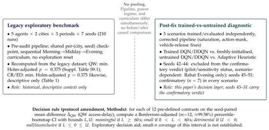
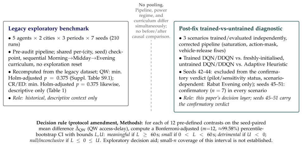
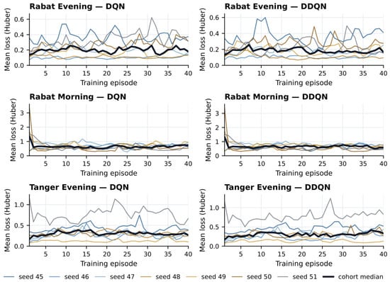
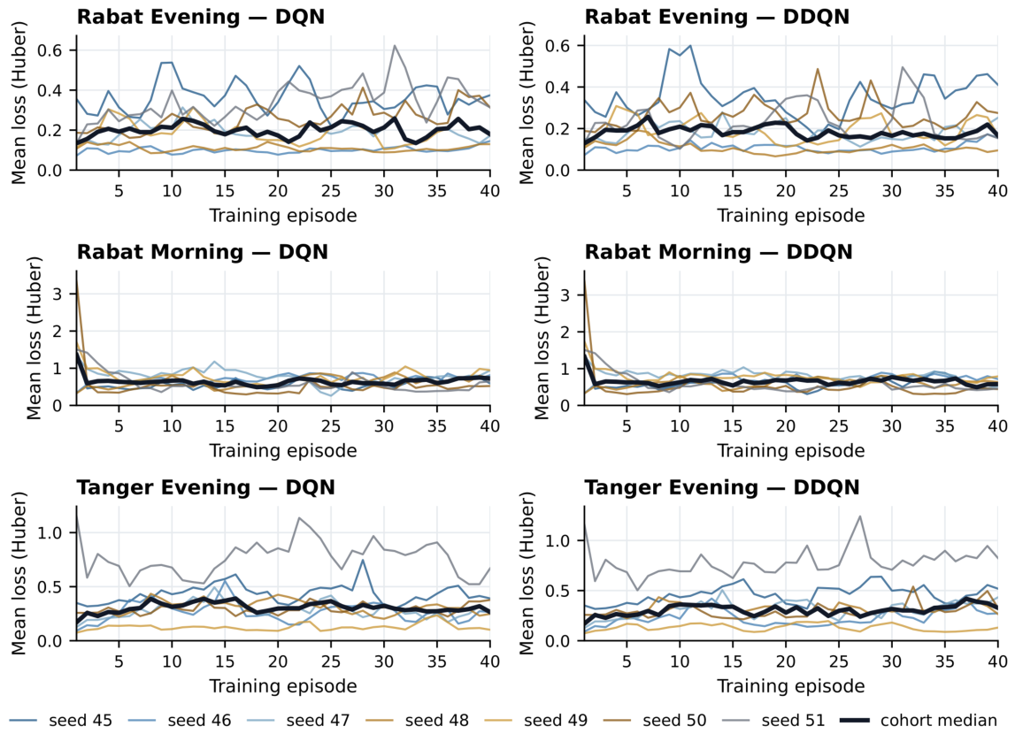
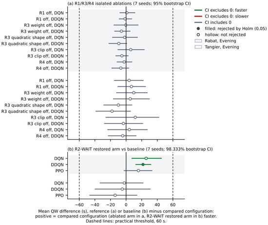
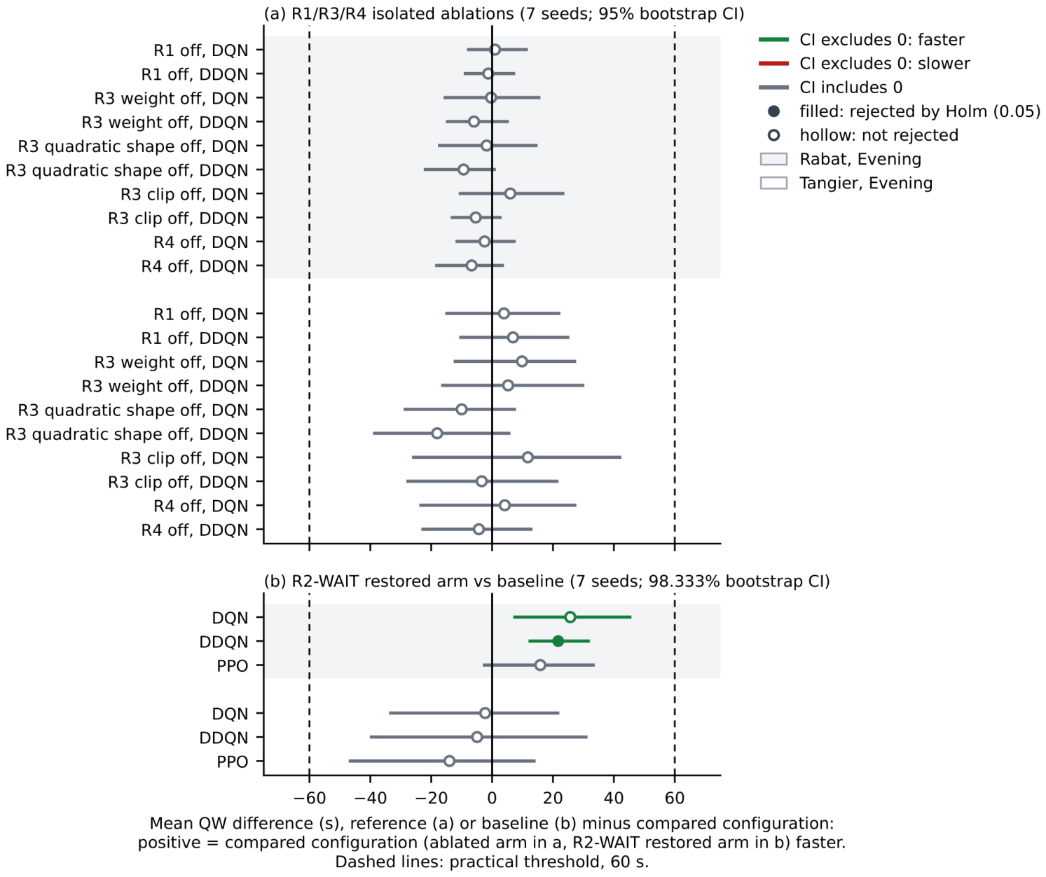
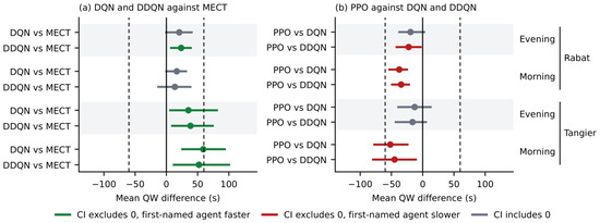
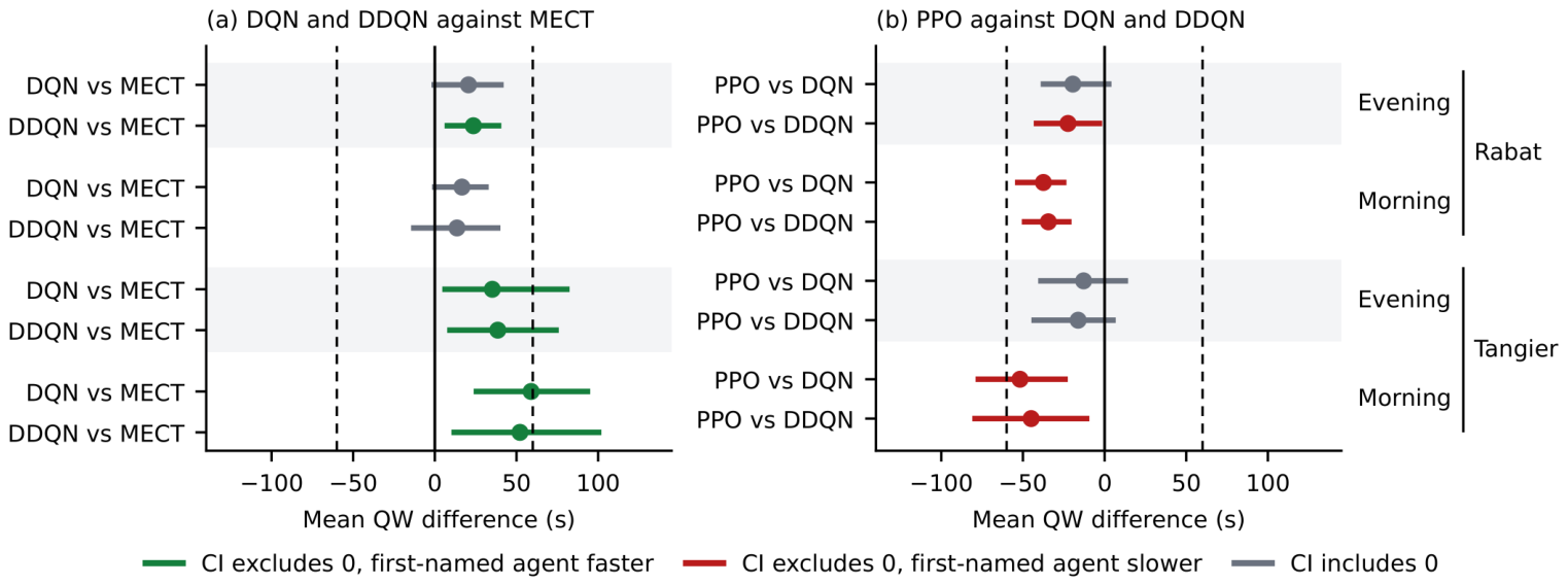

Disclaimer/Publisher’s Note: The statements, opinions and data contained in all publications are solely those of the individual author(s) and contributor(s) and not of MDPI and/or the editor(s). MDPI and/or the editor(s) disclaim responsibility for any injury to people or property resulting from any ideas, methods, instructions or products referred to in the content. |
© 2026 by the authors. Licensee MDPI, Basel, Switzerland. This article is an open access article distributed under the terms and conditions of the Creative Commons Attribution (CC BY) license.