


Abstract
Large-scale multi-objective optimization problems involve high-dimensional decision variables, vast search spaces, and conflicting objectives, which often lead to slow convergence, premature convergence, and poorly distributed solutions when conventional evolutionary algorithms operate under limited evaluation budgets. To address these challenges, this study proposes DT-MLCEA (Digital Twin-Multi-Layer Cooperative Evolutionary Algorithm), a digital twin-driven, multi-layer cooperative evolutionary algorithm. The method uses evolutionary search as its core and introduces a search-state-oriented digital twin feedback mechanism that jointly models convergence trends, diversity, distribution sparsity, stagnation, and state confidence. A multi-source adaptive control vector (MACV) is then generated to adjust key search parameters dynamically. The digital twin layer further integrates Mini-RL, Mini-AE, and Mini-Meta to refine its control recommendations and balance global exploration with local exploitation. DT-MLCEA is evaluated against LMEA, QLMGO, AMSLMOEA, and MOEA/D-RDG on LSMOP1-LSMOP9 with 100, 500, 1000, and 5000 decision variables. Across 36 problem-dimension combinations, DT-MLCEA significantly outperforms the competing algorithms in terms of HV and IGD in 28 and 24 combinations, respectively. Extended experiments on LSMOP1-LSMOP3 indicate stable performance with up to 50,000 variables. Ablation, noisy-evaluation, and parameter-sensitivity analyses further demonstrate the effectiveness of the collaborative modules.
1. Introduction
The digitalization of complex-system design and decision-making has generated numerous optimization problems involving thousands or even tens of thousands of decision variables. Examples range from the layout and routing of very-large-scale integrated circuits [1] and end-to-end learning based on deep neural networks [2] to real-time power-grid dispatch [3]. Such problems typically involve multiple conflicting objectives. Optimization problems with more than 100 decision variables are commonly referred to as large-scale multi-objective optimization problems (LSMOPs) [4]. Over several decades, evolutionary multi-objective optimization (EMO) has demonstrated the effectiveness of evolutionary algorithms for solving multi-objective problems. Classical algorithms, including NSGA-II [5], SPEA2 [6], and MOEA/D [7], perform well on low-dimensional problems, typically involving fewer than 100 decision variables, and are widely used as benchmark algorithms. However, their performance can deteriorate markedly when they are applied directly to LSMOPs because of the curse of dimensionality [8]. This limitation has become a major obstacle to the application of EMO techniques to complex real-world problems [9,10]. In 2013, Antonio and Coello proposed CCGDE3, the first algorithm specifically designed for large-scale multi-objective optimization [11]. Since then, increasing attention has been devoted to this field. According to recent reviews [12,13], existing methods can be classified into three categories according to how they handle large numbers of decision variables: decision-variable grouping methods, decision-space reduction methods, and methods based on novel search strategies. These categories are reviewed below.
The first category directly partitions large numbers of decision variables using divide-and-conquer methods (DCMs). For example, CCGDE3 randomly divides the decision variables into equally sized groups and employs third-generation generalized differential evolution [14] as the optimizer, achieving strong performance on benchmark problems. MOEA/D-VA instead groups variables according to their correlation characteristics, thereby decomposing complex problems more effectively and avoiding the limitations of random grouping when dependencies exist among variables. Subsequent studies have used clustering to divide decision variables into convergence-related and diversity-related groups [15]. However, this approach requires numerous function evaluations during grouping. To reduce this cost, the dynamic random grouping method MOEA/D-RDG [16] partitions dimensions dynamically according to heuristic information about variable dependencies rather than using fixed-size groups, substantially reducing the number of function evaluations required during evolution. WOF-MMOPSO-RDG [17] provides a hybrid framework that combines WOF [18] with the RDG strategy in a particle swarm optimizer, improving both grouping and search efficiency. Other approaches include difference-based grouping MOEAs [19,20] and methods based on relationships among variables [21,22,23]. In essence, these methods simplify a complex problem by decomposing it into independent subproblems that can be solved in parallel using existing optimizers. Their effectiveness therefore depends strongly on the decomposition strategy. Important limitations remain, including the large number of function evaluations required for grouping and relatively poor performance on problems with complex variable dependencies.
The second category reduces the decision space and performs the search in a lower-dimensional representation. One approach reformulates the original problem in a lower-dimensional space, solves the transformed problem, and maps the resulting solutions back to the original space. The Weighted Optimization Framework (WOF), for example, reduces dimensionality through problem transformation and can be combined with different evolutionary algorithms. LSMOF [24] constructs low-dimensional single-objective subproblems by establishing bidirectional associations among weight variables and then solves them using single-objective optimizers. Similarly, iLSMOA [25] reformulates the original problem as a single-objective optimization problem and uses the resulting solutions to initialize MOEA/D-DE [26]. This process is repeated to obtain the final solution set. However, problem reformulation may overemphasize convergence. To improve both effectiveness and efficiency, LMOEA-DS [27] follows the LSMOF principle to construct reference directions and randomly samples solutions along them. Another approach reduces the number of variables by exploiting relationships among them. ReMO [28], for example, uses random embedding to address LSMOPs with low intrinsic dimensionality, whereas principal component analysis has also been applied for this purpose [29]. However, both approaches rely primarily on linear relationships. Consequently, dimensionality-reduction techniques may lose important information, fail to preserve the global structure of the original search space, and become sensitive to the selected reduction model.
Both DCMs and dimensionality-reduction techniques improve efficiency by simplifying the original search space, potentially at the expense of global exploration. This trade-off has motivated a third research direction: the design of specialized search strategies that operate directly in high-dimensional spaces without grouping or dimensionality reduction. Representative approaches include competitive or direction-guided mechanisms and specialized evolutionary operators [30,31,32,33]. Although these methods are promising, they may converge slowly and require many function evaluations to obtain satisfactory solutions. More recently, online learning models [34,35] and surrogate models [36] have been introduced to guide offspring generation, accelerate convergence, and reduce the number of expensive evaluations. However, these models may incur additional computational overhead, creating a further trade-off between effectiveness and efficiency.
Within this third category, digital twin (DT) technology offers a relevant perspective because it combines virtual–physical mapping, state synchronization, online feedback, and dynamic optimization. DT technology is increasingly being applied beyond manufacturing-system modeling to complex optimization and intelligent scheduling. Tao et al. [37] reviewed the principal components, applications, and development trends of industrial digital twins and highlighted their potential to connect physical systems with virtual spaces while supporting state perception and process optimization. In learning-assisted evolutionary optimization, Song et al. [38] proposed DLES, which learns discrete search paths from evolutionary samples and reconstructs potential continuous paths using deep networks to improve subsequent candidate generation. Yu et al. [39] developed the serial multilevel-learned differential evolution algorithm (SMLDE), which combines a tightly coupled multilevel learning structure, an adaptive current-best layer, single-iteration adaptation, Cauchy perturbation, and iterative constraints to balance exploration and exploitation dynamically. Fang et al. [40] proposed an adaptive job-shop scheduling mechanism that runs reinforcement learning in a digital twin environment, improving responsiveness to dynamic disturbances through real-time state interaction and feedback. Ouahabi et al. [41] reviewed the integration of digital twins into dynamic production scheduling and noted that existing studies focus mainly on state synchronization, simulation validation, and scheduling feedback, whereas closed-loop mechanisms tightly coupled with optimization remain limited. Surrogate-assisted methods have also advanced expensive and high-dimensional multi-objective optimization. Pan et al. [42] proposed a surrogate-assisted reformulation and decomposition method to reduce actual evaluations and improve high-dimensional search efficiency. Gu et al. [43] used low-dimensional surrogates of scalarization functions to guide large-scale multi-objective evolutionary search, balancing convergence and diversity. Collectively, these studies improve complex optimization through search-path reconstruction, hierarchical individual learning, digital twin-based scheduling, and surrogate evaluation. Nevertheless, most focus on candidate generation, differential-search strategies, external modeling, or the replacement of real evaluations rather than on a lightweight algorithmic digital twin that integrates persistent state mirroring, multi-source control, online feedback, strategy memory, and tight coupling with the main evolutionary process.
In summary, a central challenge in LSMOP research is to achieve efficient global convergence, well-distributed solutions, and controllable computational cost simultaneously within a vast and complex search space. To address this challenge, this study proposes DT-MLCEA. By integrating algorithmic digital twin-driven state modeling, reinforcement learning-based parameter adjustment, meta-policy-based strategy switching, and lightweight autoencoder-based state representation, DT-MLCEA establishes a cross-layer closed-loop framework for evolutionary search. This framework coordinates perception, learning, adaptation, and stabilization to improve robustness and resource utilization in large-scale multi-objective optimization. The main contributions are as follows:
- A digital twin-driven, multi-layer cooperative evolutionary algorithm, termed DT-MLCEA, is proposed. The evolutionary algorithm acts as the sole optimization engine, while the digital twin layer monitors the population state and search trends online. This design establishes a closed loop comprising state perception, control decision-making, and evolutionary execution, thereby improving adaptability and robustness in complex high-dimensional search spaces.
- A multi-source adaptive control vector (MACV) mechanism based on information fusion is developed. The digital twin layer jointly represents population diversity, convergence trends, distribution dispersion, stagnation, and state reconstruction error to generate multidimensional control recommendations. These recommendations are integrated with a rule-based controller, lightweight reinforcement learning, and meta-policy gating to adjust crossover probability, mutation probability, elite bias, innovation strength, and contraction intensity dynamically, thereby balancing global exploration and local exploitation.
- A Lightweight Enhancement Bundle comprising Mini-RL, Mini-AE, and Mini-Meta is introduced. Mini-RL performs low-cost policy correction through a discrete state space and Q-learning; Mini-AE detects anomalies and distribution drift using state reconstruction error; and Mini-Meta switches dynamically among the Explore, Exploit, and Recover modes according to the search state. Together, these modules improve environmental adaptability and search stability without the training overhead associated with complex deep networks.
2. Related Work
Section “Large-Scale Multi-Objective Optimization Problem” introduces the fundamental concepts of LSMOPs, whereas Meanwhile, this section reviews the components related to the proposed algorithm and explains the motivation for this study.
Large-Scale Multi-Objective Optimization Problem
The mathematical formulation of an LSMOP follows that of a standard multi-objective optimization problem (MOP). An unconstrained MOP can be formulated as follows.
: The decision vector comprises n decision variables representing the parameters to be optimized. x: The corresponding space is the decision space, and the associated mapping defines the objective-function vector. n Ω F(x): ℝn → ℝm: This vector comprises several potentially conflicting objective functions. m fi(x) m: The corresponding space is called the objective space ℝm. 100 ≤ n 2 ≤ m: Problems satisfying the dimensionality condition above are referred to as LSMOPs. Because the objectives generally conflict, an MOP has no single optimal solution; instead, it has a set of trade-off solutions called Pareto-optimal solutions. The relevant Pareto-based definitions are given below:
- Pareto dominance: Given two feasible solutions, one solution dominates the other if the following conditions hold: x1 x2 fi fi(x1) ≤ fi(x2) i fj fj(x1) < fj(x2) x1. These conditions define Pareto dominance.
- Non-dominated solution: A feasible solution is non-dominated if no other feasible solution in the entire feasible set dominates it: x* x x*.
- Pareto optimality: A solution is Pareto optimal if it is non-dominated within the feasible set: x*.
- Pareto optimal set: The set of all Pareto-optimal solutions to a given LSMOP is called the Pareto-optimal set.
- Pareto front: The curve or surface formed by mapping the solutions in the Pareto-optimal set to the objective space is called the Pareto front.
These trade-off solutions constitute the Pareto-optimal set, whose image in the objective space is the Pareto front (PF). The principal objective is to identify a diverse and uniformly distributed solution set that closely approximates the true PF.
3. Algorithm
To address the high-dimensional search spaces of LSMOPs, the difficulty of balancing convergence and distribution, and the inability of fixed parameters to adapt to different search stages, this study proposes DT-MLCEA, a digital twin-driven, multi-layer cooperative evolutionary algorithm. In the current implementation, an evolutionary algorithm (EA) serves as the sole optimization engine, while an internal lightweight digital twin control layer performs online search-state perception, trend analysis, and parameter adjustment. Unlike earlier designs based on computationally intensive surrogate models or deep-network training, this implementation does not use deep surrogate prediction or generative candidate-solution mechanisms. Instead, a Lightweight Enhancement Bundle comprising Mini-RL, Mini-AE, and Mini-Meta applies low-frequency, small-magnitude, and interpretable corrections to the control recommendations generated by the digital twin layer. The resulting closed loop consists of search-state perception, parameter adjustment, and evolutionary updating.
3.1. DT-MLCEA Algorithm Design
Algorithm 1 outlines the workflow of DT-MLCEA. The procedure begins by initializing the EA core together with the lightweight digital twin module, generating an initial population P of size N, evaluating the true objective values, and setting the function-evaluation counter FE. During each generation, the DT layer is invoked at a low update frequency based on the current population state and recent performance, while an additional update can be triggered under stagnation; it then outputs parameter recommendations and mode signals for the EA search. Guided by the current MACV, the EA performs mating selection, crossover, and polynomial mutation to produce offspring Q. These offspring are evaluated using the true objective functions, optionally with batch or parallel execution, and FE is updated accordingly. Environmental selection is subsequently applied to P union Q via fast non-dominated sorting and crowding-distance estimation to form the next population. Meanwhile, HV, the stagnation indicator, and the historical state are refreshed at predefined intervals to support the DT state estimation and the next control decision. The algorithm terminates when the evaluation budget or another stopping criterion is reached, returning the final population and its non-dominated solutions.
| Algorithm 1: Main Procedure of DT-MLCEA | |||||
| Input: | N (population size), FEmax (maximum number of evaluations), Bounds Ω | ||||
| Output: | P (final population), F(P) (objective values) | ||||
| 1 | DT ←DigitalTwinController(update_interval, stagnation_threshold, control_strength) | ||||
| 2 | P ← SampleInitialPopulation(N, Ω) | ||||
| 3 | P ← InjectAnchors(P) //overwrite first ≤ 8 individuals | ||||
| 4 | F ← TrueEvaluate(P); FE ← |P|; t ← 0 | ||||
| 5 | A_dec ← empty; A_fit ← empty //external archive | ||||
| 6 | best_front ← None; best_hv ← -inf | ||||
| 7 | last_improve_gen ← 0 | ||||
| 8 | while true do | ||||
| 9 | [P, F] ← UniqueByDecision(P, F) | ||||
| 10 | [idx, rank, crowd] ← EnvironmentalSelection(F, min(N, |P|)) | ||||
| 11 | P ← P[idx]; F ← F[idx]; rank ← rank[idx]; crowd ← crowd[idx] | ||||
| 12 | F1 ← {F_i | rank_i = 0}; P1 ← {P_i|rank_i = 0} | ||||
| 13 | [A_dec, A_fit] ← UpdateArchive(A_dec, A_fit, P1, F1, N) | ||||
| 14 | HV ← NormalizedHV(F1) | ||||
| 15 | Append (t, FE, HV, |F1|, |A_fit|) to history | ||||
| 16 | if HV improves then | ||||
| 17 | best_front ← copy(F1); best_hv ← HV | ||||
| 18 | last_improve_gen ← t | ||||
| 19 | if FE ≥ FEmax then break end if | ||||
| 20 | force_refresh ← (t − last_improve_gen ≥ DT.stagnation_threshold) | ||||
| 21 | MACV ← DT.Update(t, P, F1, HV, force_refresh) | ||||
| 22 | n_off ← min(N, FEmax − FE) | ||||
| 23 | Q ← GenerateOffspring(P, F, rank, crowd, A_dec, A_fit, MACV, n_off) | ||||
| 24 | FQ ← TrueEvaluate(Q) | ||||
| 25 | FE ← FE + |Q| | ||||
| 26 | P ← P union Q | ||||
| 27 | F ← F union FQ | ||||
| 28 | t ← t + 1 | ||||
| 29 | if best_front is None then best_front ← A_fit end if | ||||
| 30 | return best_front, corresponding objective values | ||||
3.2. EA Core Evolution Mechanism
The EA core performs the evolutionary search. In the first generation, it receives the control vector generated by the DT layer. At generation t, the EA core receives the following five-dimensional multi-source adaptive control vector from the digital twin layer:
Here, and denote the mutation and crossover probabilities, respectively; denotes the elite/archive bias; denotes the innovation rate controlling exploratory offspring generation; and denotes the contraction rate controlling the reduction in the perturbation range.
Simulated binary crossover (SBX) and polynomial mutation were combined in the mutation generation stage. For the j-th decision variable of the parent individuals, random numbers are extracted, and the SBX crossover coefficient is defined as follows: xa,xb j u~U(0,1) βq,j.
The random variable follows a uniform distribution over the specified interval; u∼U(0,1) [0,1]ηc: the simulated binary crossover (SBX) distribution index controls the distribution of offspring around their parents. A larger index generates offspring closer to their parents and therefore favors local exploitation: ηc. A smaller index broadens the offspring distribution and enhances global exploration: ηc. The coefficient adjusts the search span of the decision variable during crossover and thus characterizes the strength of parental information mixing in that dimension: βq,j j.
The formula for generation of offspring variables is as follows.
where the variables represent the values of the two parents for the j-th decision variable, whereas j y1,j the remaining variables denote the corresponding offspring values: y2,j.
Subsequently, the polynomial mutation operation is performed. The random number is extracted, and the mutation perturbation term is: r~U(0,1) δj.
where denotes a uniformly distributed random variable, and r∼U(0,1) ηm the polynomial-mutation distribution index controls the magnitude of the mutation perturbation.
Apply the modulation factor and enforce the boundary restriction (for the decision variable boundary): ρt lj ≤ uj.
where the current exploration-intensity modulation factor dynamically controls the mutation step size: ρt uj. The remaining variables denote the upper and lower bounds of the j-th decision variable, respectively: lj j.
y′ = min(max(y′,lj),uj)
The environment selection stage performs a fast non-dominated sort on the merged population: Ut. If the size of the next generation is exceeded due to the addition of an individual in the frontier, the current frontier is truncated in descending order of crowding distance: N. For the first objective, the crowding distance update rule for intermediate individuals is as follows: m i.
where the variables denote the objective values of the neighboring individuals after sorting. fi+1,m fi−1,m m : The remaining terms denote the maximum and minimum values of the first objective in the current front. m ε and the final term is a small positive constant to prevent the denominator from being zero.
Algorithm 2 presents the process of generating offspring under the guidance of MACV. Firstly, parameters such as crossover, mutation, innovation and archive bias are determined based on the control vector, and the number of conventional mating and immigrant individuals is also divided; subsequently, the parent generation is constructed through tournament selection and archive guidance, and differential generation or SBX crossover is adopted according to the current settings, combined with polynomial mutation to generate offspring. Finally, the immigrant individuals are added to the population to obtain the final offspring set Q.
| Algorithm 2: Offspring Generation Under MACV | |||||||||
| Input: | P, F, rank, crowd, A_dec, A_fit, MACV, n_off | ||||||||
| Output: | Q | ||||||||
| 1 | p_m ← MACV.mutation_rate | ||||||||
| 2 | p_c ← MACV.crossover_rate | ||||||||
| 3 | b_e ← MACV.elite_bias | ||||||||
| 4 | r_i ← MACV.innovation_rate | ||||||||
| 5 | r_c ← MACV.contraction_rate | ||||||||
| 6 | r_de ← r_i | ||||||||
| 7 | r_im ← clip(r_i × (1 − r_c)) | ||||||||
| 8 | r_arc ← b_e | ||||||||
| 9 | n_im ← round(r_im × n_off), clipped to [0, n_off] | ||||||||
| 10 | n_mate ← n_off − n_im | ||||||||
| 11 | parent_idx ← BinaryTournament(rank, crowd, max(n_mate, 1)) | ||||||||
| 12 | Parents ← P[parent_idx] | ||||||||
| 13 | if A_dec not empty and r_arc > 0 then | ||||||||
| 14 | replace a subset of Parents by archive solutions | ||||||||
| 15 | pool ← P if archive empty else P union A_dec | ||||||||
| 16 | Q ← empty array of size n_off | ||||||||
| 17 | for each pair (x_a, x_b) in Parents over first n_mate positions do | ||||||||
| 18 | rand() < r_de and |pool| >= 3 then | ||||||||
| 19 | sample 3 solutions from pool | ||||||||
| 20 | y1 ← DifferentialTrial(x_a, a, b, c, scale = clip(0.35 + 0.5 × pm), cr = clip(pc)) | ||||||||
| 21 | y1 ← PolynomialMutation(y1, max(0.75 × pm, 0.02)) | ||||||||
| 22 | similarly generate y2 if needed | ||||||||
| 23 | else | ||||||||
| 24 | if rand() < pc then | ||||||||
| 25 | (y1, y2) ← SBX(x_a, x_b) | ||||||||
| 26 | else | ||||||||
| 27 | (y1, y2) ← (x_a, x_b) | ||||||||
| 28 | y1 ← PolynomialMutation(y1, pm) | ||||||||
| 29 | y2 ← PolynomialMutation(y2, pm) | ||||||||
| 30 | write offspring into Q | ||||||||
| 31 | if n_im > 0 then | ||||||||
| 32 | Q[last n_im positions] ← MakeImmigrants(n_im, A_dec, P) | ||||||||
| 33 | return Q | ||||||||
3.3. Digital Twin State Modeling
In this study, the digital twin layer is defined as an algorithmic digital twin of the evolutionary search process. It continuously synchronizes with the evolving population by monitoring convergence, diversity, sparsity, stagnation, and state confidence, and then updates the five-dimensional MACV defined in Section 3.2. Unlike conventional adaptive control based on a direct state-to-parameter mapping, the proposed mechanism maintains a persistent virtual state comprising historical windows, latent representations, action values, policy modes, and previous control information. Mini-RL estimates the expected long-term rewards of bounded control actions rather than predicting objective values. Through periodic synchronization and feedback of MACV to the EA core, the framework forms a closed loop of state perception, control decision-making, evolutionary execution, and search feedback. It is therefore characterized as a lightweight algorithm-level digital twin rather than a high-fidelity replica of a physical entity. Table 1 illustrates the differences between the Proposed Algorithm-Level Digital Twin and other methods.
Table 1.
Comparison of conventional adaptive parameter control, surrogate-assisted optimization, typical digital twins, and the algorithm-level digital twin proposed in this study.
The proposed digital twin is not a high-fidelity simulation of physical equipment but a lightweight algorithmic twin of the evolutionary search process. Its virtual entity stores not only current population metrics but also the historical window, latent states, reinforcement-learning value table, meta-policy modes, and control input from the previous time step. The twin state at generation t is defined as follows:
Tt = {st,Ht,zt,Qt,mt,at−1}
Here, st denotes the current search state; Ht is the historical state window; zt is the low-dimensional state representation; Qt is the action-value table; mt is the meta-policy mode; and at−1 is the control vector from the preceding refresh. This persistent virtual state is synchronized online with the actual population, and its control output is fed back to the next-generation search.
The search state vector is represented as:
where divt denotes diversity in the decision space, ΔHVt denotes the change in HV, spreadt denotes dispersion in the objective space, sparset denotes the proportion of sparse regions, stagt denotes the stagnation state, and conft denotes confidence in the mirrored state.
Let the population decision matrix be Xt ∈ RN×D. Diversity is then defined as follows:
The convergence trend is quantified by the difference in HV between two consecutive refresh points.
where t− denotes the most recent twin-state refresh rather than necessarily the preceding generation.
Up to 64 objective vectors are selected from the current population to form Ft. For each vector, the nearest-neighbor distance is computed as follows:
Dispersion and the sparsity ratio in the objective space are defined as follows:
where dt and σd are the mean and standard deviation of the nearest neighbor distances, respectively.
Stagnation is detected using an HV sliding window of length W = 8:
State confidence is determined jointly from fluctuations in HV and diversity and from the current distribution dispersion:
Smaller fluctuations in HV and diversity indicate a more stable search state, whereas a larger spreadt reduces confidence in the twin state.
a0 = [0.1,0.9,0.55,0.08,0.08]T
When stagt = 1, the mutation, crossover, and innovation rates are increased, whereas elite bias and contraction are reduced. When divt < 0.05 or sparset > 0.35, the mutation and innovation rates are increased. When conft > 0.75 and ΔHVt > 0, the mutation and innovation rates are reduced, while the crossover rate, elite bias, and contraction are increased to reinforce the current effective search direction.
The rule-based control vector is combined with the Mini-RL action offset as follows:
Among them:
Λ = diag(0.18,0.18,0.1,0.1,0.1)
Mini-RL estimates the long-term rewards associated with different control actions through Q-value estimation:
Thus, the twin layer responds to current indicators while using historical interactions to estimate the expected rewards of alternative control actions. The meta-policy generates an additional mode-correction term, , yielding:
To prevent abrupt changes in the control parameters, temporal smoothing is applied to the final output:
By default, the digital twin is refreshed every K = 12 generations. Synchronization occurs earlier if the stagnation counter reaches the forced-refresh threshold; otherwise, the latest control output is reused. The complete closed loop is expressed as follows:
Pt → st → Tt → at → Pt+1 → Tt+1
The digital twin layer therefore integrates multiple search-state signals into MACVt, preserves temporal continuity through boundary constraints and smoothing, and feeds the resulting vector back to the EA layer at a low frequency to coordinate exploration and exploitation.
Algorithm 3 describes the process of state modeling and control generation in the digital twin layer. Firstly, based on the current population and the first frontier, various state information such as diversity, convergence change, distribution sparsity, stagnation state and confidence level is calculated; if there is no need to refresh at the moment, the cached control vector is directly returned. Otherwise, the algorithm combines the outputs of the rule controller, Mini-AE, Mini-RL and Mini-Meta to generate and correct the current MACV, then performs constraint and smoothing processing according to different modes, and finally obtains the control parameters for the next round of evolution.
| Algorithm 3: DT State Modeling and Control | ||||
| Input: | generation t, population P_t, first-front F_t1, current HV_t, cached MACV_{t − 1} | |||
| Output: | MACV_t | |||
| 1 | div_t ← Diversity(P_t) | |||
| 2 | spread_t ← Spread(F_t1) | |||
| 3 | sparse_t ← SparseRatio(F_t1) | |||
| 4 | hv_delta_t ← HV_t − HV_{t − 1} //if no history, use 0 | |||
| 5 | stag_t ← DetectStagnation(HV window) | |||
| 6 | conf_t ← Confidence(HV window, diversity window, spread_t) | |||
| 7 | s_t ← [div_t, hv_delta_t, spread_t, sparse_t, stag_t, conf_t] | |||
| 8 | if not NeedRefresh(t, stag_t, force_refresh) then | |||
| 9 | return cached MACV | |||
| 10 | [pm_rule, pc_rule, be_rule, ri_rule, rc_rule] ← RuleController(s_t) | |||
| 11 | x_t ← [div_t, hv_delta_t, spread_t, sparse_t, conf_t, I(stag_t > 0)] | |||
| 12 | [z_t, recon_t] ← MiniAE(x_t) | |||
| 13 | a_rl ← MiniRLStep(s_t) | |||
| 14 | meta ← MetaStep(s_t, recon_t) //explore/exploit/recover | |||
| 15 | p_m ← clip(0.7 × pm_rule + 0.3 × (0.1 + a_rl.delta_pm)+ meta.delta_pm) | |||
| 16 | p_c ← clip(0.7 × pc_rule + 0.3 × (0.9 + a_rl.delta_pc)+ meta.delta_pc) | |||
| 17 | b_e ← clip(be_rule + a_rl.delta_be + meta.delta_be) | |||
| 18 | r_i ← clip(ri_rule + a_rl.delta_ri + meta.delta_ri) | |||
| 19 | r_c ← clip(rc_rule + a_rl.delta_rc + meta.delta_rc) | |||
| 20 | apply mode-dependent clamps: | |||
| 21 | if mode = recover then enforce a high r_i and a low r_c | |||
| 22 | if mode = explore then enforce a lower bound on r_i and an upper bound on b_e | |||
| 23 | if mode = exploit then enforce lower bounds on b_e and r_c when confidence is high | |||
| 24 | smooth pm and pc with previous values | |||
| 25 | cache MACV_t = {p_m, p_c, b_e, r_i, r_c} | |||
| 26 | cache mode_t separately | |||
| 27 | return MACV_t | |||
3.4. Lightweight Enhancement Bundle (Mini-RL, Mini-AE, Mini-Meta)
In DT-MLCEA, the Lightweight Enhancement Bundle does not participate directly in population evolution or candidate-solution generation. Instead, it applies small, low-frequency, and interpretable corrections to the output of the digital twin’s base controller. Mini-RL learns the long-term rewards of alternative control actions from the search state; Mini-AE extracts a low-dimensional state representation and provides an auxiliary uncertainty signal through reconstruction error; and Mini-Meta switches among exploration, exploitation, and recovery modes by combining recent search history with reconstruction error. Together, these modules improve the balance between exploration and exploitation at different search stages without incurring the training cost of complex deep networks.
Let st denote the continuous search state extracted by the digital twin at generation t, the base control vector generated by the rule-based controller, the action offset produced by Mini-RL, and the mode correction produced by Mini-Meta. The final control vector at is obtained through multi-source fusion, boundary constraints, and temporal smoothing:
In this expression, pm,t and pc,t denote the mutation and crossover rates, respectively; be,t denotes elite bias; ri,t denotes the innovation rate; and rc,t denotes the contraction rate. Mini-RL and Mini-Meta make small online adjustments to these five control components, whereas Mini-AE does not output control parameters directly but supplies latent states and reconstruction errors to Mini-Meta.
To preserve the stability of the main EA search, the rule-based controller remains the primary source of control vectors. Mini-RL supplies only scaled discrete action offsets, and Mini-Meta applies corrections of limited magnitude according to the current mode. The final output is clipped to the parameter bounds and smoothed across refresh cycles. Thus, the Lightweight Enhancement Bundle refines the decisions of the digital twin controller rather than replacing either the controller or the evolutionary algorithm.
3.4.1. Mini-RL: Lightweight Policy Modification for Low-Dimensional Discrete States
Mini-RL uses discrete states and a compact Q-table to learn small action corrections to the digital twin’s base control vector without generating candidate solutions directly. Unlike deep reinforcement learning, it uses neither neural networks nor experience replay. The Q-table is updated only after an effective refresh of the digital twin layer, thereby limiting online learning overhead. Let t- denote the preceding digital twin refresh and n the number of decisions made by Mini-RL. The continuous state is discretized as follows.
- trendt ∈ {degrade, stable, improve}, is determined by hvdelta,t.
- stagnation_flagt ∈ {0,1} By decision stagt > 0.
- low_div_flagt ∈ {0,1} By decision divt < τdiv.
Discrete state index:
state_idt = trendt × 4 + stagnation_flagt × 2 + low_div_flagt
An epsilon-greedy policy is used to select actions, and the Q-values are updated at a low frequency. The reward is defined as follows.
where denotes the reinforcement-learning reward; rt t ΔHVt the next term denotes the improvement in convergence; conft the following term denotes current-state confidence; wc the associated coefficient is the confidence-reward weight; ws the next coefficient is the stagnation-penalty weight; I(stagt > 0) the final term is the stagnation-indicator function.
rt=ΔHVt + wc × conft − ws × I(stagt > 0)
Q Update:
where the first term denotes Q(st,at) the action-value function for the current state-action pair; st at α the next parameter is the learning γ rate; the following parameter is the discount factor; and maxa′Q(st+1,a′) the final term denotes the maximum action value in the subsequent state.
3.4.2. Mini-AE: State Compression and Uncertainty Auxiliary Signals
Mini-AE is a lightweight approximation module for search-state compression and uncertainty characterization. It does not generate offspring or otherwise dominate the evolutionary process. Instead, it encodes the current search state into a compact latent representation and provides an auxiliary uncertainty signal based on reconstruction error, thereby supporting adaptive decision-making with limited computational overhead.
where xt denotes the current search-state feature vector; Wenc the next term denotes the encoder weight matrix; zt the following term denotes the encoded low-dimensional latent variable; tanh(cdot) the activation function is the hyperbolic tangent; Wdec the next term denotes the decoder weight matrix; the following term denotes the reconstructed state; zt and the final term is the latent variable.
zt = tanh(xt ⋅ Wenc)
The reconstruction error is defined as:
errvae,t: The reconstruction error serves as auxiliary uncertainty information and is supplied to Mini-Meta to determine whether the current state exhibits distributional drift or a structural anomaly. A larger error favors exploration: errvae,t.
The Mini-AE used in this paper is a lightweight state encoding and reconstruction module, whose purpose is not to build a complete probabilistic generative model, but rather to represent the current search state compactly under low computational cost, and to reflect the degree of state anomaly through reconstruction error. Its input vector is defined as:
where Istage is the stall indicator variable.
x = [div,ΔHV,spread,spread_ratio,conf,Istage] ∈ ℜ6
Unlike a standard VAE, this lightweight implementation does not use a probabilistic latent distribution, a reparameterization procedure, or a Kullback–Leibler divergence term. It uses only reconstruction error as an auxiliary signal of structural deviation.
The reconstruction error is not treated as an independent optimization objective. Instead, it is provided to Mini-Meta as an auxiliary uncertainty signal indicating distributional drift or structural anomalies in the current search state. A larger reconstruction error indicates reduced reconstructability relative to the recent reconstruction-error distribution and therefore favors exploratory control. Conversely, a persistently small error indicates a relatively stable state and favors exploitation-oriented parameter adjustments.
3.4.3. Mini-Meta: Merging Mode Gating with Strategy
Rather than using gradient-based training, Mini-Meta switches modes according to statistics computed over a sliding window of length k: k.
where denotes the mean recent change in hypervolume; k ΔHVt−k+1:t the following terms denote the HV-change sequence within the window; t − k + 1 t k and the final term denotes the sliding-window length.
where the first term is the mean population diversity over recent generations; k and the remaining terms denote the diversity sequence in the corresponding window.
where denotes the proportion of stagnant generations within the sliding window; stag_ratiot I(stag > 0) the next term is the stagnation-indicator function; mean(cdot) and the final operator denotes the mean.
stag_ratiot = mean(I(stag > 0))
The first term denotes the mean reconstruction error over the most recent k generations of Mini-AE; and the remaining terms denote the reconstruction-error sequence within the window.
Pattern determination rules:
3.4.4. Unified Fusion of Lightweight Enhancements
During fusion, the base control vector is first combined with the RL correction, after which the meta-gating correction is applied:
Clip is used for boundary stabilization. w1 + w2 = 1: This structure ensures that the enhancement module only makes “small step corrections” and does not destroy the stability of the EA main process.
Algorithm 4 describes the workflow of the lightweight enhancement module. Firstly, the algorithm discretizes the current search state and updates the RL actions through Q-learning in a low-frequency manner. At the same time, Mini-AE encodes and reconstructs the state features, and uses the reconstruction error to provide an auxiliary uncertainty signal. Subsequently, the relevant state information is written into the meta-history window, which is used by MetaGate to periodically determine whether the current state should enter the recover, explore or exploit mode, and finally outputs the RL correction amount, Meta correction amount and the corresponding mode.
| Algorithm 4: Lightweight Enhancement Bundle | |||||
| Input: | state s_t, feature x_t, previous RL state/action, meta history window | ||||
| Output: | enhancement terms and mode | ||||
| 1 | sid_t ← Discretize(s_t) | ||||
| 2 | every rl_update_interval generations: | ||||
| 3 | choose RL action by epsilon-greedy on Q[sid_t] | ||||
| 4 | reward_t ← Reward(s_t, u_t, u_{t−}) | ||||
| 5 | update Q by TD rule | ||||
| 6 | z_t ← tanh(x_t W_enc) | ||||
| 7 | xhat_t ← tanh(z_t W_dec) | ||||
| 8 | recon_t ← mean((xhat_t − x_t)2) | ||||
| 9 | push {hv_delta_t, diversity_t, stagnation_t, recon_t} into meta history | ||||
| 10 | every meta_update_interval generations: | ||||
| 11 | mode_t ← MetaGate(history) //recover/explore/exploit | ||||
| 12 | output RL deltas + meta deltas + mode_t | ||||
3.5. Information Flow and Online Update Procedure
This section describes inter-module communication and the online update schedule used to maintain an effective closed loop with minimal communication overhead. The implementation uses a hierarchical clock in which the EA drives the main loop, the DT is refreshed at a low frequency, and the enhancement modules are updated at their respective sub-frequencies. Let:
- Tbu: bottom-up update interval (EA → DT).
- Tdt: DT internal refresh interval.
- Trl: Mini-RL update interval.
- Tmeta: Mini-Meta update interval.
- stagtrigger: Stagnation force threshold.
3.5.1. Information-Flow Topology and Minimum Message Set
Only the following two core communication links are retained:
- (1)
- EA → DT (State uplink)
msgup,t = {t,Pt,Ft,metricst,stagt}
- (2)
- DT → EA (Control delivery)
3.5.2. Event Triggering and Low-Frequency Updates
DT refresh condition:
where indicates whether the digital twin state must be refreshed at the current generation; need_refresh_t t: the next term denotes the current generation; tlast_refresh: the following term denotes the most recent DT refresh; Tdt denotes the DT refresh interval; stagt: the next term denotes the current stagnation level; stagtrigger and the final term denotes the stagnation-trigger threshold.
need_refresh_t = (t − tlast_refresh ≥ Tdt) ∨ (stagt ≥ stagtrigger)
3.5.3. Offline Initialization and Online Learning
To mitigate cold-start instability, each submodule uses a combination of offline initialization and lightweight online updating:
- Offline phase (one-time).
The Q-table, projection matrix, and gating thresholds are initialized using default values or a small warm-start sample:
θ0 = Init(θ;config,optional_offline_data)
- Online phase (per generation/divider)
Only the required statistics and lightweight parameters are updated; no computationally intensive backpropagation is performed:
where minibatcht learning uses the sliding-window history rather than large-scale experience replay.
θt+1 = OnlineUpdate(θt,minibatcht,low_cost_rule)
3.5.4. Function-Evaluation Counting and Consistency
During online optimization, the true function-evaluation count is incremented only when the true objective function is called:
FEt+1 = FEt + |Qt|
Any predicted value is used only as an auxiliary signal and is not counted as a true function evaluation. This convention ensures a consistent evaluation budget across algorithms.
4. Experimental Design
The performance of DT-MLCEA is evaluated on the LSMOP benchmark suite using LMEA, QLMGO [44], AMSLMOEA [45], and MOEA/D-RDG as comparison algorithms. LMEA is a representative evolutionary algorithm for LSMOPs. QLMGO uses Q-learning to switch adaptively between random reverse learning and chaotic search, thereby balancing global exploration and local exploitation in high-dimensional decision spaces. AMSLMOEA is designed specifically for large-scale multi-objective optimization and emphasizes convergence and solution quality under limited evaluation budgets. MOEA/D-RDG is a decomposition-based large-scale multi-objective evolutionary algorithm that improves distribution and convergence through variable analysis and global diversity restoration. These algorithms provide complementary baselines for evaluating the convergence, distribution, and stability of DT-MLCEA in large-scale settings.
4.1. Algorithm Setup
For a fair comparison, all algorithms used the same evaluation budget. In the baseline experiments, the population size was 100 and the maximum number of function evaluations was 10,000. The comparison algorithms used the parameter settings recommended in their original publications or standard configurations from publicly available implementations, without additional tuning of their core mechanisms. Specifically, LMEA used conventional real-coded crossover and mutation, with a crossover probability of 1.0 and distribution indices of 20 for both simulated binary crossover (SBX) and polynomial mutation (PM). QLMGO, AMSLMOEA, and MOEA/D-RDG used the standard parameters specified in their original methods or public implementations. DT-MLCEA used the official implementation described in this study, comprising an evolutionary algorithm layer and a lightweight digital twin control layer that adjusts crossover, mutation, innovation, and elite-bias parameters adaptively. The official experimental implementation does not include the earlier deep surrogate architecture; consequently, the three-layer fully connected surrogate model with 10 neurons per layer and Swish activation was not used. All experiments were conducted under Windows 11 on a laptop equipped with an AMD Ryzen 9 7940HX processor, an NVIDIA RTX 4060 Laptop GPU, and 40 GB of memory. Python 3.8 was used for all algorithmic evaluations. The full list of hyperparameters used in DT-MLCEA is provided in Table A1.
4.2. Problem Setup
All LSMOP1-LSMOP9 instances were configured with three objectives and 100, 500, 1000, or 5000 decision variables to evaluate performance at different scales. These problems exhibit diverse characteristics, including low intrinsic dimensionality, deception, and multimodality. Performance was assessed using inverted generational distance (IGD) and hypervolume (HV), for which smaller and larger values indicate better performance, respectively.
IGD was calculated using the reference-front generation procedure defined in the original description of the standard LSMOP suite. For HV, the objective values of the non-dominated solutions were normalized to [0,1] using the ideal and nadir points of the true reference front to account for differences in objective scale. The reference point was then fixed at (1.2, 1.2, 1.2), ensuring consistent HV calculation across problems. IGD is used exclusively for post hoc performance evaluation and does not influence the evolutionary search, parameter adaptation, archive updating, or final solution selection.
To account for stochastic variation, each algorithm was run independently 20 times for every problem and dimension. Differences between each comparison algorithm and DT-MLCEA were assessed using the Wilcoxon rank-sum test at a significance level of 0.05. The Benjamini–Hochberg false-discovery-rate correction was applied separately to the 144 HV and 144 IGD comparisons (9 problems × 4 dimensions × 4 comparison algorithms), with the FDR threshold set to 0.05. In Table 2 and Table 3, “+” indicates that a comparison algorithm performs significantly better than DT-MLCEA after correction (q < 0.05), “−” indicates significantly worse performance, and the absence of a symbol indicates no significant difference. Values in parentheses are standard deviations over the 20 runs.
Table 2.
HV performance of the algorithms on the benchmark problems.
Table 3.
IGD performance of the algorithms on the benchmark problems.
4.3. Benchmark Results
Table 2 and Table 3 report the HV and IGD results, respectively, for DT-MLCEA, LMEA, QLMGO, AMSLMOEA, and MOEA/D-RDG on LSMOP1-LSMOP9. Each value is the mean over 20 independent runs, and the best result for each instance is shown in bold. For HV, DT-MLCEA was significantly better in 132 of the 144 pairwise comparisons, significantly worse than QLMGO in 4 comparisons, and significantly worse than LMEA or MOEA/D-RDG in 8 comparisons. It significantly outperformed all comparison algorithms on 28 problem-dimension combinations. For IGD, DT-MLCEA was significantly better in 130 of 144 pairwise comparisons, significantly worse than AMSLMOEA in 4 comparisons on LSMOP5, and significantly worse than QLMGO in 10 comparisons on LSMOP5, LSMOP8, and LSMOP9. It significantly outperformed all comparison algorithms on 24 problem-dimension combinations.
These results can be attributed primarily to the adaptive collaborative regulation mechanism of DT-MLCEA. Multi-source information fusion enables the algorithm to identify the current search state and compensate for underrepresented regions of the front while maintaining convergence. Parameter smoothing and boundary constraints also reduce abrupt intergenerational oscillations and improve search stability. Together, these mechanisms allow DT-MLCEA to balance HV and IGD across most large-scale test settings while maintaining solution distribution and stability as the problem dimension increases.
Figure 1 compares the IGD trajectories of the algorithms on 1000-dimensional LSMOP1-LSMOP3 under the limited evaluation budget. DT-MLCEA maintains comparatively low IGD values on all three problems, indicating stable convergence and strong overall performance relative to LMEA, QLMGO, AMSLMOEA, and MOEA/D-RDG. On LSMOP1 and LSMOP2, DT-MLCEA, QLMGO, and AMSLMOEA continue to improve during the later search stages. On LSMOP3, DT-MLCEA and AMSLMOEA also continue to improve, whereas QLMGO stabilizes after an initial decrease during the middle and later stages. Overall, DT-MLCEA exhibits strong convergence and competitiveness on these test problems.
Figure 1.
IGD convergence curves (d = 1000).
An overall comparison was performed using the Friedman test across the 36 problem–dimension instances. Significant differences were observed among the algorithms for both HV (x2 = 84.956, p = 1.55 × 10⁻¹⁷) and IGD (x2 = 85.079, p = 1.46 × 10⁻¹⁷). Figure 2 presents the average ranks, showing that DT-MLCEA ranked first for both HV and IGD, with average ranks of 1.333 and 1.389, respectively, while QLMGO ranked second for IGD with an average rank of 2.139. These results indicate that DT-MLCEA is highly competitive across the tested problems and dimensions.
Figure 2.
Average ranks of the compared algorithms based on the Friedman test for HV and IGD.
4.4. Scalability Testing
To evaluate scalability under greater computational resources, the maximum number of function evaluations was increased to 100,000 and the decision-space dimensionality was extended to 10,000, 15,000, 20,000, 30,000, and 50,000. The experiments were conducted on LSMOP1-LSMOP3, with all other settings retained from Section 4.1 and Section 4.2. Runtime and memory consumption were also recorded as the number of decision variables increased to characterize the practical computational cost of high-dimensional optimization.
As shown in Figure 3, the IGD trajectories of all algorithms generally stabilize when the maximum evaluation budget is increased to 100,000. Relative to the results obtained with 10,000 evaluations, DT-MLCEA, QLMGO, and AMSLMOEA achieve further IGD reductions on LSMOP1 and LSMOP2, with particularly clear improvements for DT-MLCEA and AMSLMOEA; LMEA and MOEA/D-RDG change only slightly. Most algorithms reach a relatively stable stage after approximately 30,000 evaluations on LSMOP1 and LSMOP2. On LSMOP3, however, DT-MLCEA, QLMGO, and AMSLMOEA continue to improve even at 100,000 evaluations, indicating that further convergence toward the Pareto front may be possible under a larger budget. Overall, DT-MLCEA obtains high-quality solution sets under low-to-moderate budgets and remains competitive as the budget increases.
Figure 3.
IGD convergence curves under a budget of 100,000 function evaluations.
Figure 4 and the Kendall τ-b test reveal distinct dimensional trends among the algorithms on LSMOP1-LSMOP3. For DT-MLCEA, IGD decreases significantly with dimension on LSMOP1 and LSMOP2 (τ = −1.000 and −1.000; p = 0.0167 and 0.0167), indicating no deterioration over the tested dimensional range. The trend on LSMOP3 is not significant (τ = −0.200, p = 0.8167), indicating broadly stable performance. LMEA shows no significant trend on any of the three problems: IGD decreases slightly on LSMOP1 and LSMOP3 (τ = −0.200 and −0.600) and remains nearly unchanged on LSMOP2 (τ = 0.000), with all p-values exceeding 0.05. QLMGO exhibits significant decreases on LSMOP1 and LSMOP2 (τ = −1.000 and −1.000; p = 0.0167 and 0.0167) but a significant increase on LSMOP3 (τ = 1.000, p = 0.0167), indicating deterioration on the latter problem. AMSLMOEA exhibits no significant trend on LSMOP1 or LSMOP2 (τ = −0.200 and −0.400; p = 0.8167 and 0.4833) but improves significantly on LSMOP3 (τ = −1.000, p = 0.0167). MOEA/D-RDG shows no significant trend: its IGD increases on LSMOP1 and LSMOP3 (τ = 0.600 and 0.600) and increases slightly on LSMOP2 (τ = 0.400), but all corresponding p-values exceed 0.05.
Figure 4.
IGD performance of the algorithms as the number of decision variables increases.
As shown in Figure 5, DT-MLCEA required more computation time than several comparison algorithms in the representative high-dimensional tests, with the difference increasing as the number of variables rose from 10,000 to 50,000. Its runtime increased from 25.08 to 67.00 s, whereas the runtimes of LMEA and MOEA/D-RDG increased from 6.25 to 10.30 s and from 9.56 to 22.16 s, respectively. However, DT-MLCEA did not exhibit the highest peak memory consumption. At 10,000 and 50,000 variables, it used 177.5 and 383.0 MB, respectively, lower than the corresponding values for QLMGO (253.4 and 759.4 MB) and AMSLMOEA (231.9 and 723.7 MB). Thus, DT-MLCEA’s additional computational cost at high dimensions is reflected primarily in runtime rather than memory consumption.
Figure 5.
Runtime and memory usage of the compared algorithms with increasing numbers of decision variables.
4.5. Robustness Testing
Two complementary experiments were performed to evaluate stability under uncertainty: noisy re-evaluation of the final solution set and noise injection during optimization. Both experiments were independently repeated 20 times, and the reported results are based on the mean values across these runs. The former assesses the sensitivity of the obtained solution sets to perturbations in objective values, whereas the latter continuously adds zero-mean Gaussian noise during objective-function evaluations to assess performance under noisy search conditions. The experiments used 1000-dimensional LSMOP1–LSMOP3, with all other settings retained from Section 4.1 and Section 4.2.
First, each algorithm was run in a noise-free environment, after which its final non-dominated solution set was repeatedly re-evaluated under noise. The corresponding HV and IGD values were then calculated. Figure 6 shows that the algorithms exhibit different trends across the test problems, with local fluctuations occurring at low noise levels for some methods. Overall, the HV and IGD values of DT-MLCEA remain within relatively narrow ranges, while its IGD distributions show low medians and limited dispersion. The resulting solution sets therefore demonstrate a degree of stability against objective-value perturbations. However, this experiment assesses only the post-search sensitivity of the final solution sets and does not directly characterize robustness during noisy optimization.
Figure 6.
Robustness evaluation of the algorithms.
Second, zero-mean Gaussian noise was added to every objective-function evaluation during optimization. After each run, the final solution set was re-evaluated using the noise-free objective functions to prevent direct contamination of the performance indicators. Figure 7 reports the mean IGD values obtained from 20 independent runs under different online noise levels. As the noise level increases, IGD generally increases on LSMOP1 and LSMOP2 for most algorithms, indicating that persistent evaluation errors affect the search direction and environmental selection. The effects on LSMOP3 are smaller, demonstrating that noise sensitivity is problem-dependent. DT-MLCEA maintains relatively low mean IGD values across all three problems and performs particularly well on LSMOP1 and LSMOP2. Its IGD increases slightly with noise on LSMOP3 but remains comparatively stable. QLMGO and the other algorithms also exhibit stability at some noise levels, although their responses vary across problems.
Figure 7.
IGD performance of the compared algorithms under different online objective-noise levels on LSMOP1–LSMOP3.
Together, these two experiments distinguish the post-search sensitivity of the final solution sets from the stability of the optimization process under noisy evaluations. Based on the mean results of 20 independent runs, DT-MLCEA maintains relatively low IGD values and tolerates moderate objective-evaluation noise under the tested conditions.
4.6. Ablation Experiments
To assess the contribution of each core module, the full DT-MLCEA model was compared with five variants: w/o DT, w/o RL, w/o AE, w/o Meta, and w/o EnhOp. All variants used the same problem settings, population size, and maximum evaluation budget. The experiments covered 1000-dimensional LSMOP1-LSMOP9 and used HV and IGD as performance indicators; the results are reported in Table 4. Each variant was run independently 20 times. Differences between each ablated variant and the full model were evaluated using the Wilcoxon rank-sum test at a significance level of 0.05, followed by Benjamini–Hochberg FDR correction for 45 comparisons for each metric (q < 0.05). In Table 4, “+” and “−” indicate that an ablated variant performs significantly better or worse than the full model, respectively.
Table 4.
Ablation results of DT-MLCEA in terms of HV, IGD, and execution time.
Overall, the full model obtains the best HV and IGD values across LSMOP1-LSMOP9, indicating that its performance arises from the combined contributions of the digital twin control layer and the Lightweight Enhancement Bundle. For HV, removing Mini-RL produces the largest reduction. On LSMOP1, LSMOP2, and LSMOP6, for example, HV decreases from 2.762 × 10⁻², 2.552 × 10⁻², and 2.893 × 10⁻² for the full model to 2.237 × 10⁻², 2.067 × 10⁻², and 2.343 × 10⁻² without Mini-RL, respectively. This result indicates that RL-based regulation contributes substantially to front quality and search intensity. For IGD, removing Mini-AE generally produces the smallest degradation, whereas removing Mini-Meta produces the largest. On LSMOP3, LSMOP5, and LSMOP9, the IGD values of the full model are 6.058 × 10⁻¹, 5.762 × 10⁻¹, and 6.720 × 10⁻¹, whereas those of w/o Meta are 6.967 × 10⁻¹, 6.626 × 10⁻¹, and 7.728 × 10⁻¹, respectively. This result highlights the contribution of Mini-Meta to search stability, state-drift control, and approximation quality. Removing either the DT layer or EnhOp also degrades both HV and IGD systematically, confirming their contributions to state perception and search enhancement. In terms of runtime, w/o RL is the fastest variant (24.81 s), whereas w/o DT is the slowest (26.74 s). Thus, although some modules introduce additional operations, they are associated with more stable and substantial performance gains. Overall, the ablation study indicates that DT-MLCEA benefits from the combined effects of digital twin control, reinforcement-learning-based regulation, lightweight state representation, meta-policy gating, and enhanced search operators. Mini-RL has the largest influence on HV, Mini-Meta contributes most strongly to IGD, and Mini-AE, DT, and EnhOp support robustness and overall performance on the tested high-dimensional problems.
4.7. Sensitivity Analysis
Sensitivity analysis was conducted on six core DT-MLCEA parameters using LSMOP1–LSMOP3 with 100, 500, 1000, and 5000 decision variables. Each parameter setting was independently evaluated twenty times, and Figure 8 reports the mean IGD values over these twenty runs. The dotted lines in the figure indicate the numerical values used by the algorithm. Performance variation under each setting was quantified using the coefficient of variation (CV) of IGD. The mean CV for population size is 4.465%, indicating comparatively high sensitivity. The corresponding mean CVs for mutation probability, DT control strength, RL reward weight, AE latent-space dimension, and the Meta threshold are 0.607%, 0.663%, 0.565%, 0.643%, and 0.709%, respectively, all below 1%. Thus, except for population size, DT-MLCEA maintains relatively stable IGD values across the tested parameter ranges and does not require selection from a narrow interval. The default settings (population_size = 100, Pm = 0.18, DT control strength = 1.0, RL reward weight = 1.8, latent_dim = 5, and Meta threshold = 0.22) lie within regions of stable and favorable performance. These results suggest that the observed performance is primarily attributable to the digital twin control, strategy adaptation, and collaborative modules rather than to problem-specific parameter tuning.
Figure 8.
Single-Factor Sensitivity Analysis on LSMOP1–LSMOP3 across Four Dimensions.
To examine interactions between parameters, a two-parameter sensitivity analysis was performed for DT control strength and the Meta reconstruction-error threshold (Figure 9). Across the tested parameter combinations, the CVs of IGD are 4.013%, 4.345%, and 1.733% for LSMOP1, LSMOP2, and LSMOP3, respectively, all below 5%. None of the plots exhibits consistent deterioration as either parameter changes. DT-MLCEA therefore maintains relatively stable performance across the tested combinations of DT control strength and the Meta threshold, indicating limited dependence on a specific pair of parameter values.
Figure 9.
Two-parameter sensitivity analysis of mean IGD with respect to DT control strength and Meta reconstruction-error threshold on LSMOP1–LSMOP3.
5. Conclusions
This study proposes DT-MLCEA, a lightweight digital twin-based cooperative framework for large-scale multi-objective optimization. Unlike earlier designs based on computationally intensive models, DT-MLCEA combines an EA search process with lightweight DT control. Mini-RL, Mini-AE, and Mini-Meta provide low-overhead collaborative regulation, enabling adaptive adjustment of crossover rate, mutation rate, and search intensity through state monitoring, mode switching, and temporal smoothing. This mechanism balances convergence and distribution in complex high-dimensional search spaces. Experiments on LSMOP1-LSMOP9 with 100, 500, 1000, and 5000 decision variables show that DT-MLCEA significantly outperforms LMEA, QLMGO, AMSLMOEA, and MOEA/D-RDG in terms of HV and IGD on 28 and 24 problem-dimension combinations, respectively. The results also indicate stable HV, limited IGD degradation as dimensionality increases, and robustness to the tested noise conditions.
Future work will investigate how problem-specific heuristics and domain knowledge can be used to customize digital twin fidelity and guidance vectors for real-world LSMOP applications, such as feature selection. Multi-agent reinforcement learning may also be incorporated to coordinate guidance vectors, mutation and crossover operators, and key parameters, while interpretable preferences and online noise models may further improve applicability and efficiency in complex environments.
Author Contributions
Conceptualization, D.L. and W.B.; methodology, D.L., F.G. and W.B.; software, C.C., H.W., H.L. and Y.S.; validation, D.L., F.G., C.C., H.W., H.L., Y.S., X.L. and M.D.; formal analysis, D.L., F.G. and X.L.; investigation, D.L., F.G., C.C., H.W., H.L., Y.S., X.L. and M.D.; resources, D.L., F.G., C.C. and H.W.; data curation, D.L., C.C., H.W., H.L., Y.S., X.L. and M.D.; writing—original draft preparation, D.L., F.G., C.C., H.W., H.L. and Y.S.; writing—review and editing, D.L., F.G., C.C., H.W., H.L., Y.S., X.L., M.D. and W.B.; visualization, D.L., C.C., H.W., H.L. and Y.S.; supervision, D.L., F.G. and W.B.; project administration, D.L. and W.B.; funding acquisition, W.B. All authors have read and agreed to the published version of the manuscript.
Funding
This research was funded by the Lhasa Regional Collaborative Innovation Special Project (“Unveiling the List and Appointing Talents” Program), grant number LSKJ202463.
Data Availability Statement
The data presented in this study are openly available at https://github.com/621-time/DT-MLCEA (accessed on 6 August 2026).
Acknowledgments
The authors thank the Lhasa Regional Collaborative Innovation Special Project for its support.
Conflicts of Interest
Author Haiyang Lyu and Yutao Song are employed by Nanjing Hanhai Fuxi Defense Technology Co., Ltd. The remaining authors declare that the research was conducted in the absence of any commercial or financial relationships that could be construed as a potential conflict of interest.
Appendix A
Appendix A.1
This appendix lists the principal hyperparameter values used for each DT-MLCEA module in the reported experiments. These parameters affect search behavior, convergence, and final solution quality and are therefore provided to facilitate reproducibility and interpretation.
Table A1.
Principal hyperparameters used in the experiments.
Appendix A.2
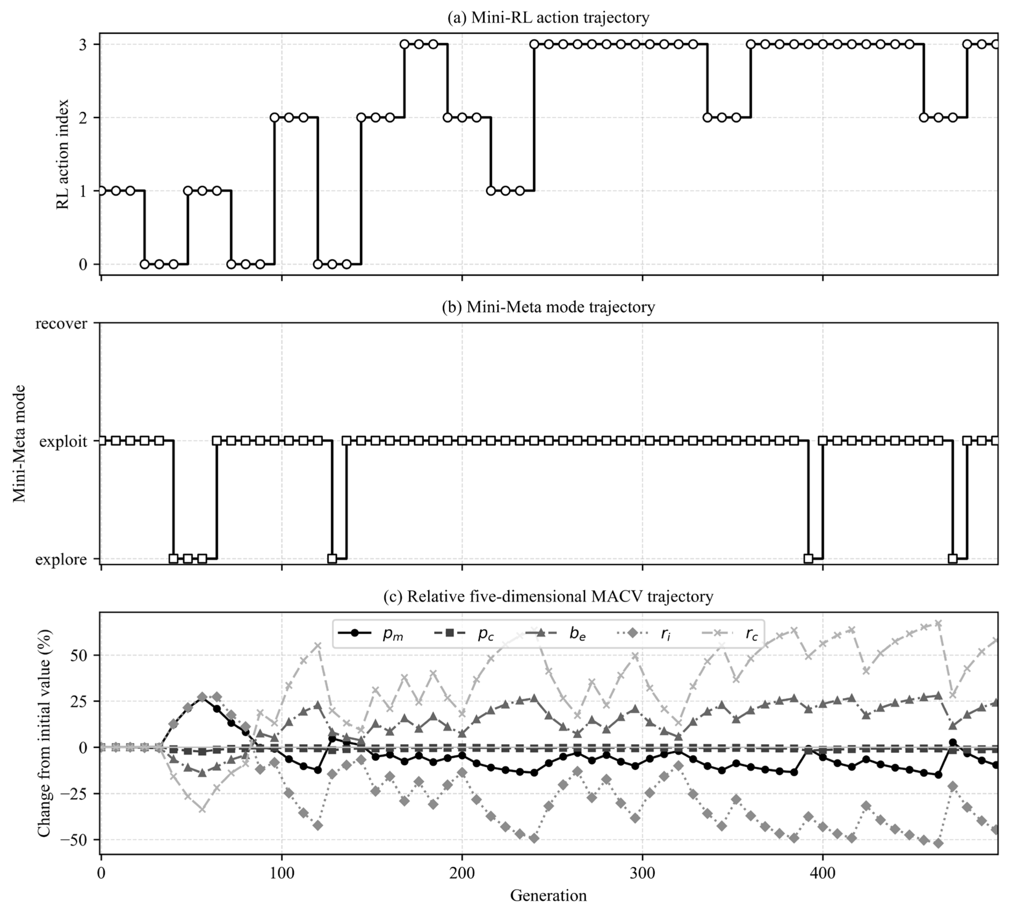
Figure A1 presents a representative control trajectory of DT-MLCEA on LSMOP3 with 1000 variables and 50,000 function evaluations. Mini-RL dynamically switches among four bounded actions, while Mini-Meta activates the exploration mode at several search stages. The resulting MACV variations remain bounded, illustrating the problem-dependent interaction between RL-based corrections and meta-policy gating.
Figure A1.
Trajectories of Mini-RL actions, Mini-Meta modes, and relative MACV changes on LSMOP3 under 50,000 function evaluations.
Appendix A.3
Following the Friedman omnibus test, two-sided paired Wilcoxon signed-rank tests were conducted between DT-MLCEA and each competing algorithm using the mean HV and IGD values from the 36 problem-dimension instances. Holm correction was applied separately to the four comparisons for each metric. As shown in Table A2, DT-MLCEA achieved significantly better overall performance than all four competitors for both HV and IGD at the 0.05 significance level. The rank-biserial effect sizes ranged from 0.802 to 1.000 for HV and from 0.375 to 1.000 for IGD, indicating large effects in most comparisons, although the advantage over QLMGO in IGD was comparatively modest.
Table A2.
Holm-adjusted post hoc comparisons between DT-MLCEA and the competing algorithms across 36 problem-dimension instances.
References
- Rajeswari, P.; Theodore Chandra, S.; Smitha, S. Efficient k-way partitioning of very-large-scale integration circuits with evolutionary computation algorithms. Bull. Electr. Eng. Inform. 2024, 13, 4002–4007. [Google Scholar] [CrossRef] [Scilit]
- Yu, C.; Wang, Y.; Tang, C.; Feng, W.; Lv, J. EU-Net: Automatic U-Net neural architecture search with differential evolutionary algorithm for medical image segmentation. Comput. Biol. Med. 2023, 167, 107579. [Google Scholar] [CrossRef] [Scilit] [PubMed]
- Albogamy, F.R.; Paracha, M.Y.I.; Hafeez, G.; Khan, I.; Murawwat, S.; Rukh, G.; Khan, S.; Khan, M.U.A. Real-time scheduling for optimal energy optimization in smart grid integrated with renewable energy sources. IEEE Access 2022, 10, 35498–35520. [Google Scholar] [CrossRef] [Scilit]
- Tian, Y.; Si, L.; Zhang, X.; Cheng, R.; He, C.; Tan, K.C.; Jin, Y. Evolutionary large-scale multi-objective optimization: A survey. ACM Comput. Surv. 2021, 54, 1–34. [Google Scholar] [CrossRef] [Scilit]
- Deb, K.; Pratap, A.; Agarwal, S.; Meyarivan, T. A fast and elitist multiobjective genetic algorithm: NSGA-II. IEEE Trans. Evol. Comput. 2002, 6, 182–197. [Google Scholar] [CrossRef] [Scilit]
- Zitzler, E.; Laumanns, M.; Thiele, L. SPEA2: Improving the Strength Pareto Evolutionary Algorithm; Computer Engineering and Networks Laboratory, ETH Zurich: Zurich, Switzerland, 2001. [Google Scholar]
- Zhang, Q.; Li, H. MOEA/D: A multiobjective evolutionary algorithm based on decomposition. IEEE Trans. Evol. Comput. 2007, 11, 712–731. [Google Scholar] [CrossRef] [Scilit]
- Tian, Y.; Lu, C.; Zhang, X.; Tan, K.C.; Jin, Y. Solving large-scale multiobjective optimization problems with sparse optimal solutions via unsupervised neural networks. IEEE Trans. Cybern. 2021, 51, 3115–3128. [Google Scholar] [CrossRef] [Scilit] [PubMed]
- Ma, X.; Liu, F.; Qi, Y.; Wang, X.; Li, L.; Jiao, L.; Yin, M.; Gong, M. A multiobjective evolutionary algorithm based on decision variable analyses for multiobjective optimization problems with large-scale variables. IEEE Trans. Evol. Comput. 2016, 20, 275–298. [Google Scholar] [CrossRef] [Scilit]
- Durillo, J.J.; Nebro, A.J.; Coello, C.A.C.; García-Nieto, J.; Luna, F.; Alba, E. A study of multiobjective metaheuristics when solving parameter scalable problems. IEEE Trans. Evol. Comput. 2010, 14, 618–635. [Google Scholar] [CrossRef] [Scilit]
- Antonio, L.M.; Coello, C.A.C. Use of cooperative coevolution for solving large scale multiobjective optimization problems. In Proceedings of the 2013 IEEE Congress on Evolutionary Computation; IEEE: Piscataway, NJ, USA, 2013; pp. 2758–2765. [Google Scholar]
- Hong, W.J.; Yang, P.; Tang, K. Evolutionary computation for large-scale multi-objective optimization: A decade of progresses. Int. J. Autom. Comput. 2021, 18, 155–169. [Google Scholar] [CrossRef] [Scilit]
- Zille, H. Large-Scale Multi-Objective Optimisation: New Approaches and a Classification of the State-of-the-Art. Ph.D. Thesis, Otto von Guericke University Magdeburg, Magdeburg, Germany, 2019. [Google Scholar]
- Kukkonen, S.; Lampinen, J. GDE3: The third evolution step of generalized differential evolution. In Proceedings of the 2005 IEEE Congress on Evolutionary Computation; IEEE: Piscataway, NJ, USA, 2005; Volume 1, pp. 443–450. [Google Scholar]
- Zhang, X.; Tian, Y.; Cheng, R.; Jin, Y. A decision variable clustering-based evolutionary algorithm for large-scale many-objective optimization. IEEE Trans. Evol. Comput. 2018, 22, 97–112. [Google Scholar] [CrossRef] [Scilit]
- Song, A.; Yang, Q.; Chen, W.N.; Zhang, J. A random-based dynamic grouping strategy for large scale multi-objective optimization. In Proceedings of the 2016 IEEE Congress on Evolutionary Computation; IEEE: Piscataway, NJ, USA, 2016; pp. 468–475. [Google Scholar]
- Liu, R.; Li, Y.; Liu, J. A random dynamic grouping based weight optimization framework for large-scale multi-objective optimization problems. Swarm Evol. Comput. 2020, 55, 100684. [Google Scholar] [CrossRef] [Scilit]
- Zille, H.; Ishibuchi, H.; Mostaghim, S.; Nojima, Y. A framework for large-scale multiobjective optimization based on problem transformation. IEEE Trans. Evol. Comput. 2018, 22, 260–275. [Google Scholar] [CrossRef] [Scilit]
- Sander, F.; Zille, H.; Mostaghim, S. Transfer strategies from single- to multi-objective grouping mechanisms. In Proceedings of the Genetic and Evolutionary Computation Conference; ACM: New York, NY, USA, 2018; pp. 729–736. [Google Scholar]
- Li, M.; Wei, J. A cooperative co-evolutionary algorithm for large-scale multi-objective optimization problems. In Proceedings of the Genetic and Evolutionary Computation Conference Companion; ACM: New York, NY, USA, 2018; pp. 1716–1721. [Google Scholar]
- Zhang, J.; Wei, L.; Fan, R.; Sun, H.; Hu, Z. Solve large-scale many-objective optimization problems based on dual analysis of objective space and decision space. Swarm Evol. Comput. 2022, 70, 101045. [Google Scholar] [CrossRef] [Scilit]
- Yang, L.; Liu, J.; Li, F.; Tan, S.; Zheng, T.; Liu, Y. A matrix adaptation evolution strategy based evolution algorithm for large-scale many-objective optimization. In Proceedings of the 2020 Chinese Control and Decision Conference; IEEE: Piscataway, NJ, USA, 2020; pp. 2518–2523. [Google Scholar]
- Zhang, M.; Li, W.; Zhang, L.; Jin, H.; Mu, Y.; Wang, L. A Pearson correlation-based adaptive variable grouping method for large-scale multi-objective optimization. Inf. Sci. 2023, 639, 118737. [Google Scholar] [CrossRef] [Scilit]
- He, C.; Li, L.; Tian, Y.; Zhang, X.; Cheng, R.; Jin, Y.; Yao, X. Accelerating large-scale multiobjective optimization via problem reformulation. IEEE Trans. Evol. Comput. 2019, 23, 949–961. [Google Scholar] [CrossRef] [Scilit]
- He, C.; Cheng, R.; Tian, Y.; Zhang, X. Iterated problem reformulation for evolutionary large-scale multiobjective optimization. In Proceedings of the 2020 IEEE Congress on Evolutionary Computation; IEEE: Piscataway, NJ, USA, 2020; pp. 1–8. [Google Scholar]
- Li, H.; Zhang, Q. Multiobjective optimization problems with complicated Pareto sets, MOEA/D and NSGA-II. IEEE Trans. Evol. Comput. 2009, 13, 284–302. [Google Scholar] [CrossRef] [Scilit]
- Qin, S.; Sun, C.; Jin, Y.; Tan, Y.; Fieldsend, J. Large-scale evolutionary multiobjective optimization assisted by directed sampling. IEEE Trans. Evol. Comput. 2021, 25, 724–738. [Google Scholar] [CrossRef] [Scilit]
- Qian, H.; Yu, Y. Solving high-dimensional multi-objective optimization problems with low effective dimensions. In Proceedings of the Thirty-First AAAI Conference on Artificial Intelligence; AAAI Press: Washington, DC, USA, 2017; Volume 31. [Google Scholar]
- Liu, R.; Ren, R.; Liu, J. A clustering and dimensionality reduction based evolutionary algorithm for large-scale multi-objective problems. Appl. Soft Comput. 2020, 89, 106120. [Google Scholar] [CrossRef] [Scilit]
- Wang, X.; Zhang, K.; Wang, J.; Jin, Y. An enhanced competitive swarm optimizer with strongly convex sparse operator for large-scale multiobjective optimization. IEEE Trans. Evol. Comput. 2022, 26, 859–871. [Google Scholar] [CrossRef] [Scilit]
- Zhang, X.; Zheng, X.; Cheng, R.; Qiu, J.; Jin, Y. A competitive mechanism based multi-objective particle swarm optimizer with fast convergence. Inf. Sci. 2018, 427, 63–76. [Google Scholar] [CrossRef] [Scilit]
- Tian, Y.; Zheng, X.; Zhang, X.; Jin, Y. Efficient large-scale multiobjective optimization based on a competitive swarm optimizer. IEEE Trans. Cybern. 2020, 50, 3696–3708. [Google Scholar] [CrossRef] [Scilit] [PubMed]
- Qi, S.; Wang, R.; Zhang, T.; Huang, W.; Qing, F.; Hu, T.; Wang, L. A Thompson sampling-based sparse evolutionary operator for sparse large-scale multiobjective optimization. IEEE Trans. Evol. Comput. 2025, 29, 2521–2536. [Google Scholar] [CrossRef] [Scilit]
- Mittal, S.; Saxena, D.K.; Deb, K.; Goodman, E.D. A learning-based innovized progress operator for faster convergence in evolutionary multi-objective optimization. ACM Trans. Evol. Learn. Optim. 2021, 2, 1–29. [Google Scholar] [CrossRef] [Scilit]
- Liu, S.; Li, J.; Lin, Q.; Tian, Y.; Tan, K.C. Learning to accelerate evolutionary search for large-scale multiobjective optimization. IEEE Trans. Evol. Comput. 2023, 27, 67–81. [Google Scholar] [CrossRef] [Scilit]
- Chugh, T.; Jin, Y.; Miettinen, K.; Hakanen, J.; Sindhya, K. A surrogate-assisted reference vector guided evolutionary algorithm for computationally expensive many-objective optimization. IEEE Trans. Evol. Comput. 2018, 22, 129–142. [Google Scholar] [CrossRef] [Scilit]
- Tao, F.; Zhang, H.; Liu, A.; Nee, A.Y. Digital twin in industry: State-of-the-art. IEEE Trans. Ind. Inform. 2019, 15, 2405–2415. [Google Scholar] [CrossRef] [Scilit]
- Song, Y.; Wang, K.; Zhan, Z.-H.; Lei, Z.; Gao, S. Learning-assisted search path reconstruction empowers evolution algorithm for optimization. IEEE Trans. Evol. Comput. 2026, 30, 321–332. [Google Scholar] [CrossRef] [Scilit]
- Yu, J.; Wang, K.; Lei, Z.; Cheng, J.; Gao, S. Serial multilevel-learned differential evolution with adaptive guidance of exploration and exploitation. Expert Syst. Appl. 2024, 255, 124646. [Google Scholar] [CrossRef] [Scilit]
- Fang, W.; Zhang, H.; Qian, W.; Guo, Y.; Li, S.; Liu, Z.; Liu, C.; Hong, D. An adaptive job shop scheduling mechanism for disturbances by running reinforcement learning in digital twin environment. J. Comput. Inf. Sci. Eng. 2023, 23, 051013. [Google Scholar] [CrossRef] [Scilit]
- Ouahabi, N.; Chebak, A.; Kamach, O.; Laayati, O.; Zegrari, M. Leveraging digital twin into dynamic production scheduling: A review. Robot. Comput.-Integr. Manuf. 2024, 89, 102778. [Google Scholar] [CrossRef] [Scilit]
- Pan, L.; Lin, J.; Wang, H.; He, C.; Tan, K.C.; Jin, Y. Computationally expensive high-dimensional multiobjective optimization via surrogate-assisted reformulation and decomposition. IEEE Trans. Evol. Comput. 2025, 29, 921–935. [Google Scholar] [CrossRef] [Scilit]
- Gu, H.; Wang, H.; He, C.; Yuan, B.; Jin, Y. Large-scale multiobjective evolutionary algorithm guided by low-dimensional surrogates of scalarization functions. Evol. Comput. 2025, 33, 309–334. [Google Scholar] [CrossRef] [Scilit] [PubMed]
- Sarangi, P.; Mohapatra, S.; Mohapatra, P. A novel Q-learning-inspired Mountain Gazelle Optimizer for solving global optimization problems. Int. J. Mach. Learn. Cybern. 2025, 16, 6167–6213. [Google Scholar] [CrossRef] [Scilit]
- Zhang, X.; Chen, D.; Ge, F.; Zou, F.; Cui, L. Large-scale multiobjective competitive swarm optimizer algorithm based on regional multidirectional search. Complex Intell. Syst. 2025, 11, 51. [Google Scholar] [CrossRef] [Scilit]
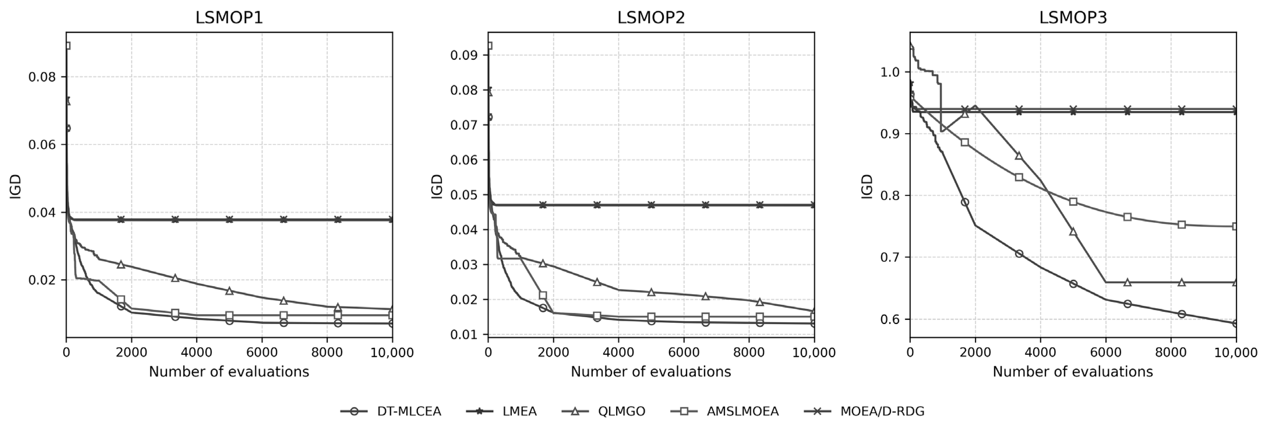
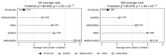
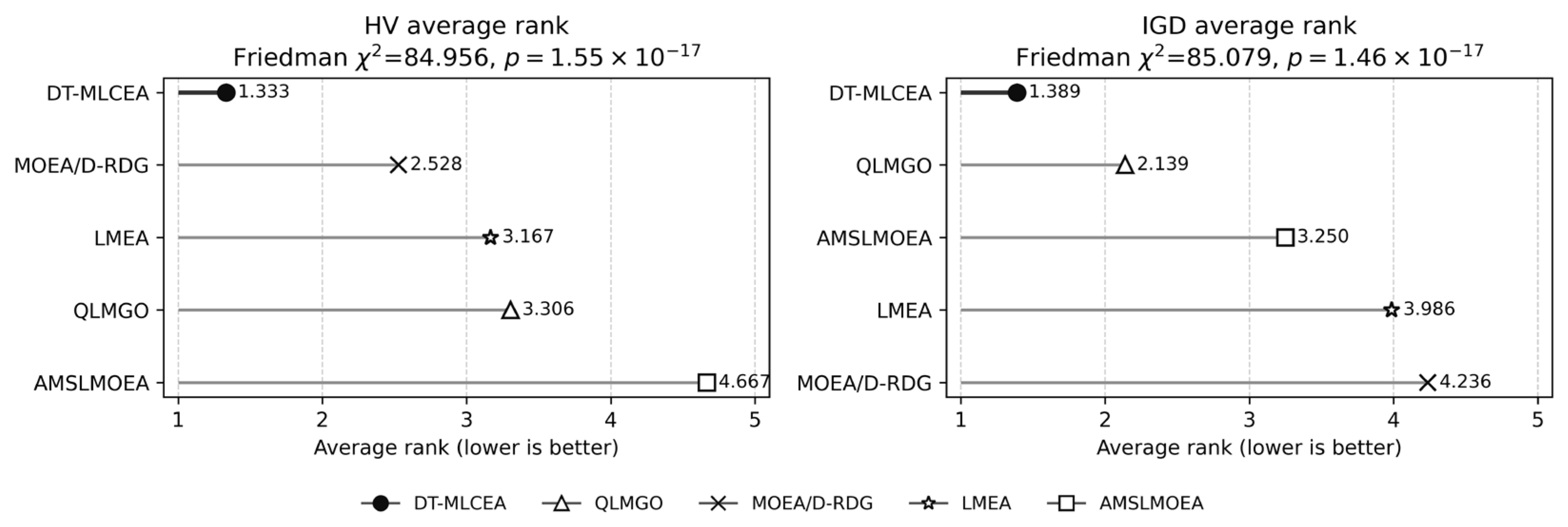
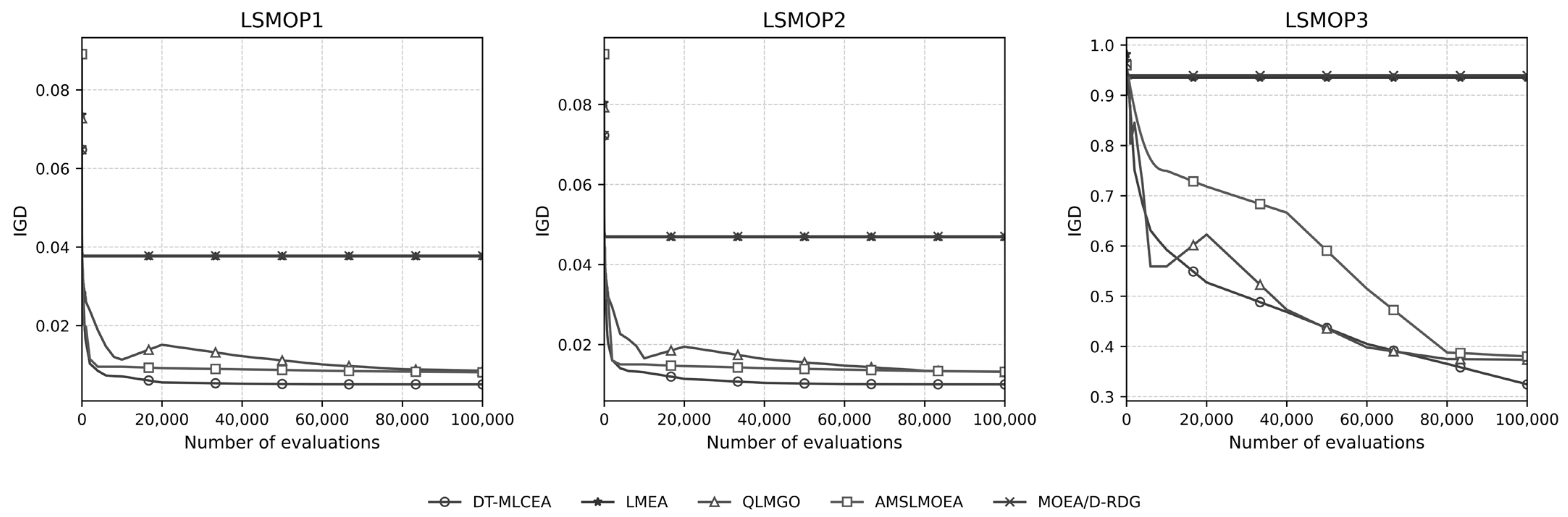
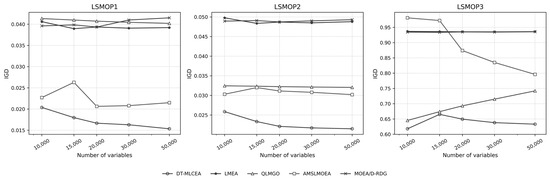
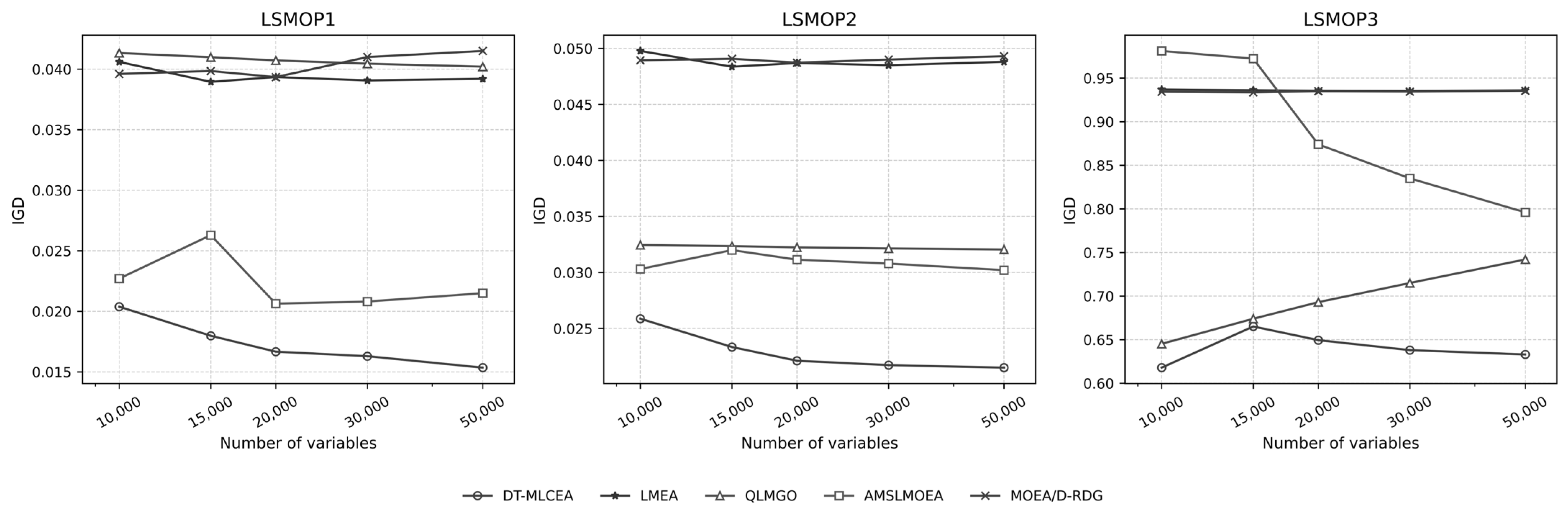
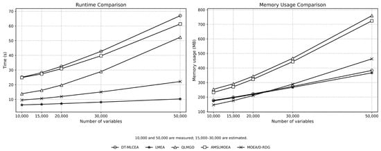
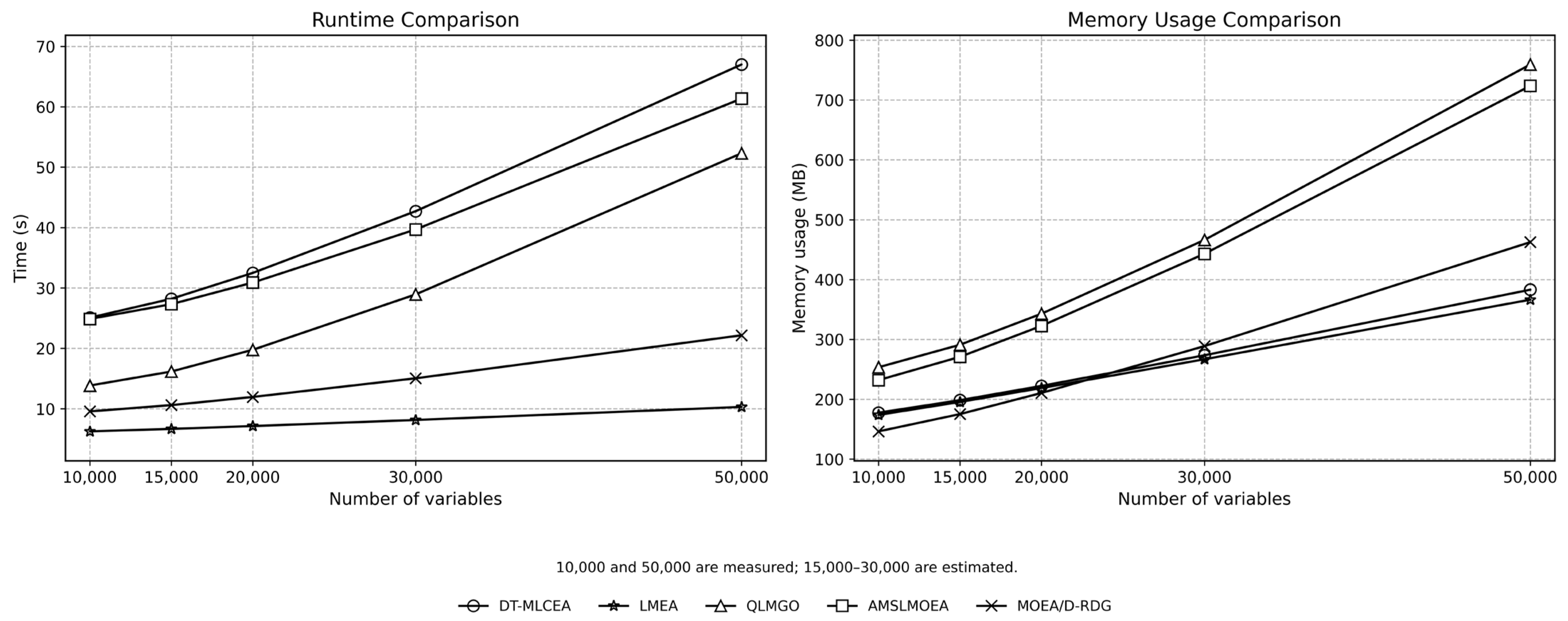
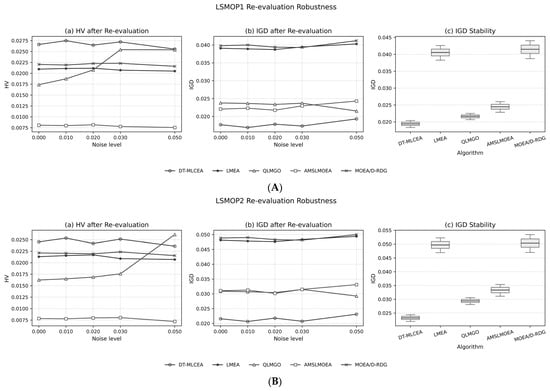
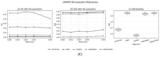
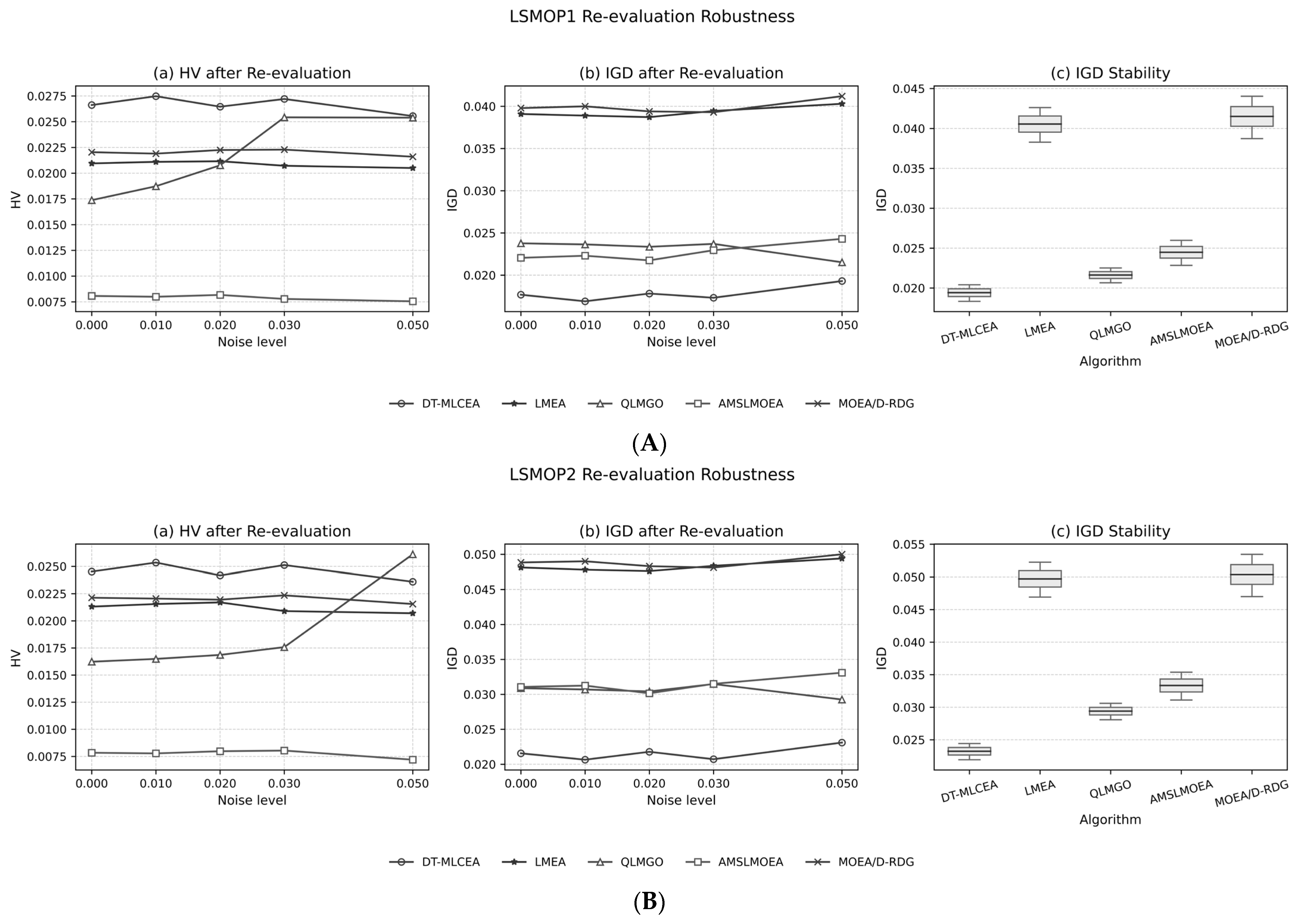
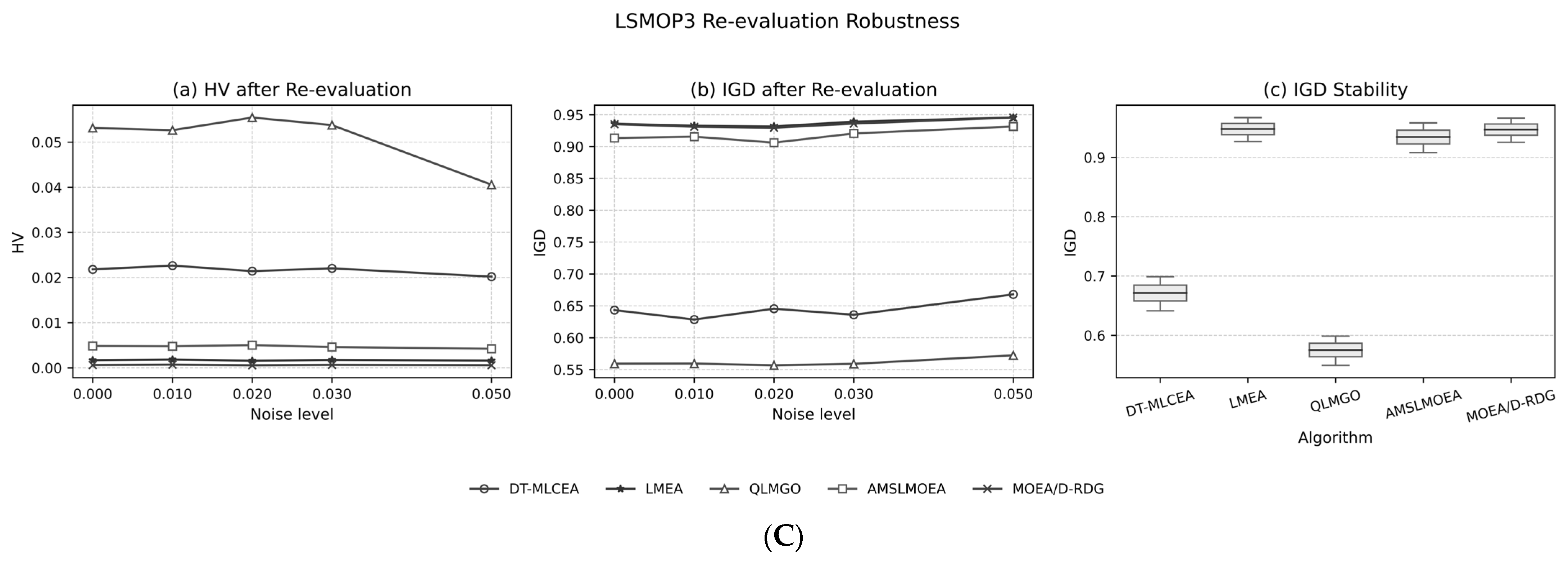
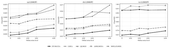
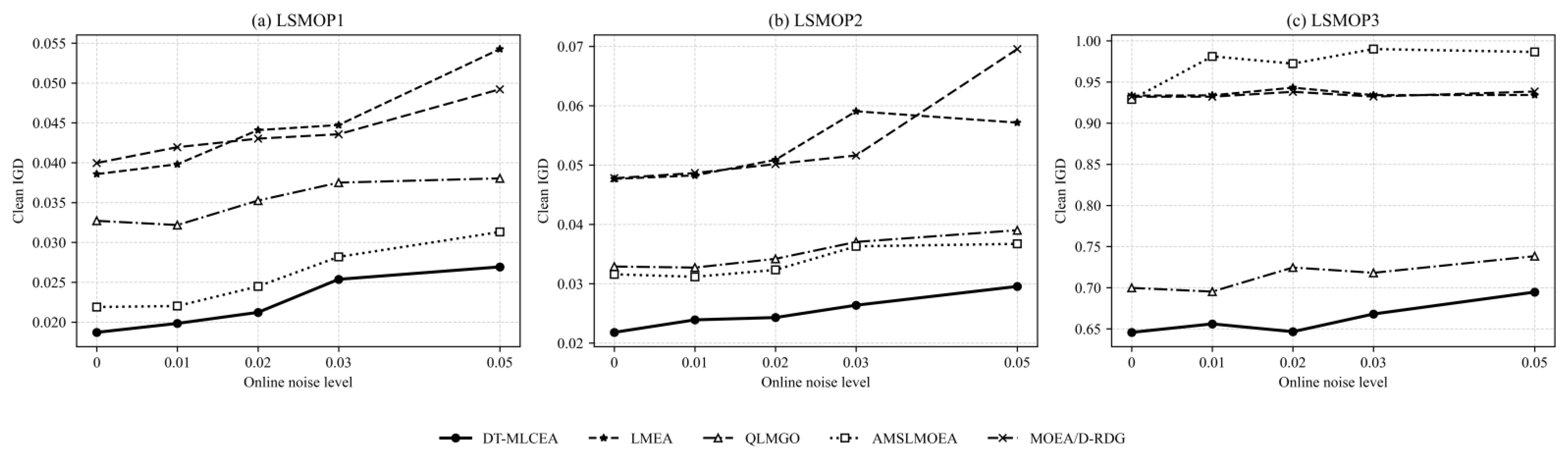
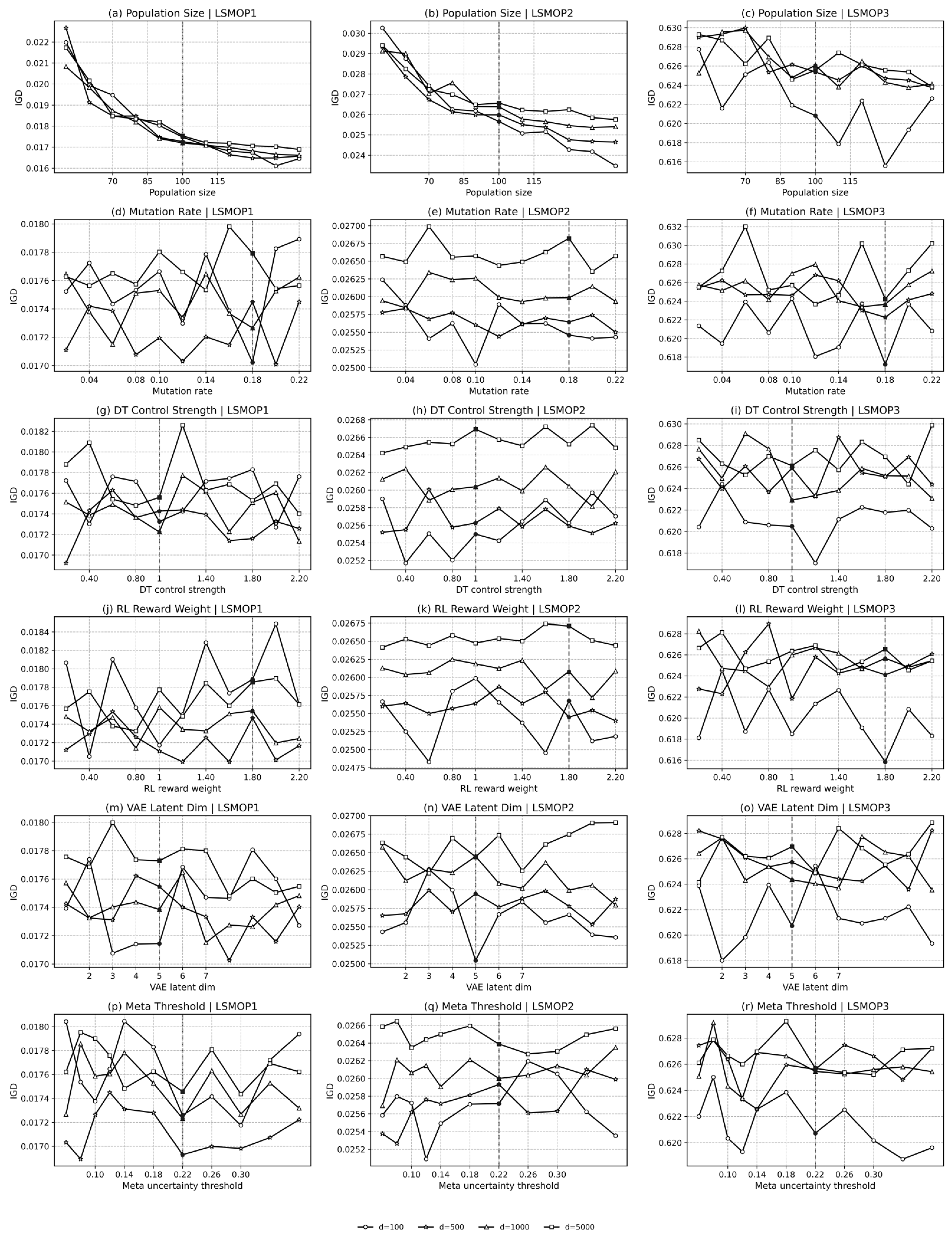
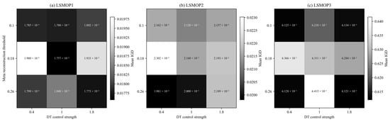
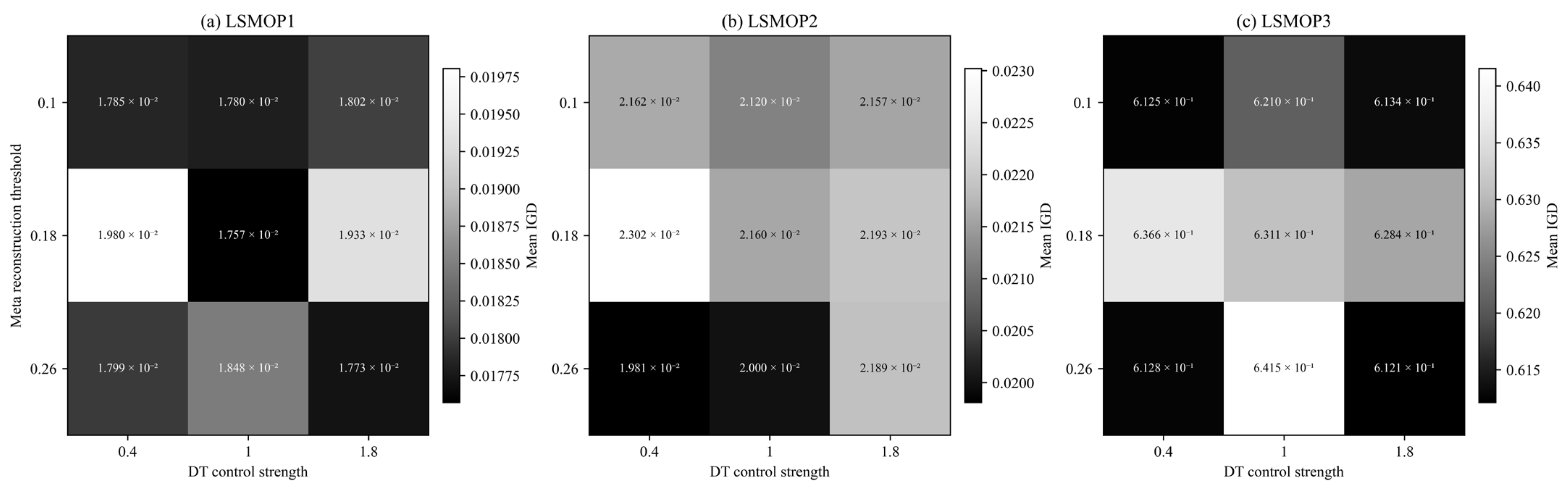

Disclaimer/Publisher’s Note: The statements, opinions and data contained in all publications are solely those of the individual author(s) and contributor(s) and not of MDPI and/or the editor(s). MDPI and/or the editor(s) disclaim responsibility for any injury to people or property resulting from any ideas, methods, instructions or products referred to in the content. |
© 2026 by the authors. Licensee MDPI, Basel, Switzerland. This article is an open access article distributed under the terms and conditions of the Creative Commons Attribution (CC BY) license.