


Abstract
It is well known that biomedical imaging analysis plays a crucial role in the healthcare sector and produces a huge quantity of data. These data can be exploited to study diseases and their evolution in a deeper way or to predict their onsets. In particular, image classification represents one of the main problems in the biomedical imaging context. Due to the data complexity, biomedical image classification can be carried out by trainable mathematical models, such as artificial neural networks. When employing a neural network, one of the main challenges is to determine the optimal duration of the training phase to achieve the best performance. This paper introduces a new adaptive early stopping technique to set the optimal training time based on dynamic selection strategies to fix the learning rate and the mini-batch size of the stochastic gradient method exploited as the optimizer. The numerical experiments, carried out on different artificial neural networks for image classification, show that the developed adaptive early stopping procedure leads to the same literature performance while finalizing the training in fewer epochs. The numerical examples have been performed on the CIFAR100 dataset and on two distinct MedMNIST2D datasets which are the large-scale lightweight benchmark for biomedical image classification.
1. Introduction
In recent years, the healthcare field has experienced a massive growth in the acquisition of digital biomedical images due to a pervasive increase in ordinary and preventive medical exams. In view of this amount of medical data, new methods based on machine learning (ML) and deep learning (DL) have therefore become necessary. The application of ML and DL techniques to the biomedical imaging field can promote the development of new diagnostics and treatments, making it a challenging area of investigation. In particular, image classification represents one of the main problems in the biomedical imaging context. Its aim is to arrange medical images into different classes to help physicians in disease diagnosis. ML and DL methods are employed to predict the class membership of the unknown data instance, based on the class membership of the training set data, which is known. If the learning procedure performs a good classification, a proper automatic diagnosis of a disease can be achieved, starting only from the medical image.
From a mathematical point of view, given a training set of n instances, a learning approach to the image classification involves the solution of a minimization problem of the form
where F is the so-called loss function and it computes the difference between the actual ground-truth and predicted values, n is the cardinality of the training set and d is the number of features. Each denotes the loss function related to the i-th instance of the training set. Because n can be a very large number, it is prohibitively expensive to compute all the terms of the objective function or its gradient. Moreover, the whole dataset may be too large to be completely stored in memory. Finally, in the online learning setting, where the dataset is not available from the beginning in its completeness but is acquired during the learning process, it is impossible to work with . In all these cases, the minimization problem is faced by exploiting stochastic approximations of the gradient that lead to the use of stochastic gradient (SG) methods [1]. Given at each iteration k a sample of size randomly and uniformly chosen from , the SG algorithm to solve problem (1) can be written as
where is a positive parameter called the learning rate (LR) and the stochastic direction is computed as
The sample is the mini-batch at the k-th iteration and its cardinality is the mini-batch size (MBS). In order to accelerate the convergence rate of the SG method, a momentum term [2] can be added to the iteration (2). In more detail, chosen and setting , the momentum version of the SG scheme has the following form:
where is the positive LR.
In general, to design efficient and accurate ML or DL methodologies, it is needed to properly set the hyperparameters connected to the algorithm chosen for the training phase, particularly the LR and the MBS. We define the hyperparameters of a learning method as those parameters which are not trained during the learning process but are set a priori as the input data. In the literature, there are different philosophies to approach the problem of setting the hyperparameters. One of these is related to the Neural Architecture Search (NAS) area [3], which explores the best configurations related to the optimization hyperparameters before the beginning of the training. However, there also exist techniques that directly address the search during the training phase, including static rules, i.e., rules that do not depend on the training phase, and dynamic rules, which only operate under certain conditions connected to the training phase itself. Regarding the LR and the MBS, the class of dynamic rules is preferable. Indeed, a variable LR strategy allows starting the iterative process with higher LR values than those employed close to the local minimum. As for the MBS, a standard approach is to dynamically increase it along the iterations, without however reaching the whole dataset in order to comply with the architectural constraints and control the possible data redundancy. There also exist techniques for decreasing the LR while the MBS is increasing.
Together with suitable choices of both the LR and the MBS, the training phase can be optimized by means of an early stopping technique. Given a validation set (VS), namely a subset of examples held back from training the model, standard early stopping procedures are based on the so-called patience parameter criterion. In more detail, if, after a number of epochs equal to the value of the patience, the loss function computed on the VS has not been reduced, the training is stopped even if the maximum number of epochs is not reached.
The aim of this paper is twofold. First, we combine the previously described strategies to reduce the training time. Indeed, we suggest a dynamic combined technique to select the LR and the MBS by modifying classical early stopping procedures. In particular, if a decrease in the loss function on the validation set is not achieved after the patience time, the patience value itself can be reduced, the learning rate is decreased and/or the mini-batch size is increased and the training is allowed to continue until the values of the learning rate and the mini-batch are acceptable from a practical point of view. Secondly, we test the SG algorithm with momentum, equipped with a such developed rule for the selection of the LR and MBS hyperparameters, in training an artificial neural network (ANN) for biomedical image classification problems. We remark that the dynamical early stopping procedure we describe in this paper can be adopted for general image classification problems. Moreover, it is worth highlighting that the suggested approach does not belong to the class of NAS hyperparameters procedures. Indeed, unlike the proposed scheme, NAS techniques aim to set good hyperparameters values at the beginning of the training phase and to keep them fixed until convergence. On the other hand, the hyperparameters selection rule developed in this work is adaptive because the hyperparameters connected to the optimizer can be conveniently changed during the training phase. This can have benefits in terms of both the performance and computational and energy savings from a GreenAI (Artificial Intelligence) perspective.
The paper is organized as follows. In Section 2, we present a brief survey about the state-of-the-art approaches to fix both the LR and the MBS hyperparameters. Section 3 is devoted to describing a novel technique to dynamically adjust the LR and/or the MBS, using the VS. Section 4 reports the results of the numerical experiments on standard and biomedical image classification problems, aimed to evaluate the effectiveness of the proposed approach. In Section 5, in addition to the conclusions, the current directions of research that we are pursuing to expand and complete the work carried out are illustrated.
2. Related Works
The aim of this section is to recall the standard techniques to select the LR and the MBS in stochastic gradient methods typically employed for ML and DL methodologies.
2.1. Standard LR Selection Rules
Properly setting the LR in stochastic gradient algorithms is an important issue and there exist many attempts in the literature to address it. Indeed, inappropriate values for the LR can lead to two different scenarios: a too small fixed value often implies a very slow learning process, while a too high fixed value can make the method divergent. In general, choosing a fixed LR along the iterative process is not suitable, also because the convergence of standard first-order stochastic schemes is ensured if the LR is properly bounded by the Lipschitz constant of the gradient of the objective function [1]. Unfortunately, this constant is often not known.
As for a variable LR rule, several works in the literature show that, from a practical point of view, modifying the LR during the learning process can bring benefits for both ML and DL applications [4,5]. In order to guarantee convergence, the SG schemes require the LR to be chosen as a value of a diminishing sequence, i.e., . However, this choice would practically lead to a too rapid reduction in the LR by giving rise to the interruption of the learning process in a few iterates. For this reason, in practice, the so-called LR annealing can be adopted: with this strategy, the LR is decreased along the iterations but with a much slower speed. The basic idea of the LR annealing is to diminish the LR after some iterations from the beginning of the learning process, in an automatic and non-adaptive way. This technique is widely used in the most recent ANN for segmentation and other tasks [6,7,8]. For example, in [7], the authors use the LR annealing technique, with a YOLO architecture, for the detection and the localization of lung nodules from low-dose CT scans. Even in biomedical contexts, where the dataset size is often limited, LR annealing techniques have been shown to be effective. In [9], the authors demonstrate that the suggested LR annealing strategy improves the image classifiers performance, in terms of both the accuracy and training time, on a set of dermatological diagnostic images with an unbalanced nature.
2.2. Standard MBS Selection Rules
In [10], Masters and Luschi point out that modern DL training is typically based on mini-batch SG optimization. While the use of large mini-batches increases the available computational parallelism, small-batch training has been shown to provide a better generalization performance and allows a significantly smaller memory footprint, which might also be exploited to improve machine throughput. For this reason, the authors stress that, for the learning process, it is crucial to choose a proper MBS selection technique that allows the method to achieve a high accuracy while reducing the time spent on the learning phase as much as possible.
In the context of standard ML, several authors suggest a linear growth of the MBS to allow the process of reaching the entire dataset, while others (see, e.g., [11]) propose a hybrid approach. The hybrid approach consists of starting the iterative process with an SG method (by exploiting its property of decreasing the objective function especially in the first iterations) and then moving onto a deterministic scheme (by taking advantage of its stability and avoiding an oscillating behavior around the minimum point). Obviously, these techniques cannot be applied to every setting, but only to offline learning frameworks and/or datasets of limited size.
For the DL approaches, the MBS is often selected as powers of 2 (commonly 32, 64 and 128) with the aim of facilitating the use of internal memories of accelerators, such as a Graphics Processing Unit (GPU) and Field-Programmable Gate Array (FPGA). However, besides static MBS selection strategies, simply driven by heuristics or hardware constraints, there exist other adaptive ones driven by the learning process itself [12,13]. For example, in [12], the authors design a practical SG method capable of learning the optimal batch size adaptively throughout its iterations for strongly convex and smooth functions. On the other hand, in [13], the authors propose a method to dynamically use the VS to set the MBS. The impact of a suitable MBS selection procedure on the effectiveness of DL schemes has been also analyzed in the field of medical applications. In [14], the authors studied the effect of the MBS on the performance of CNNs employed to classify histopathology images. They empirically found that when the LR values are high, a large MBS performs better than with a small LR. Moreover, lowering the learning rate and decreasing the batch size allow the network to train better, especially in the case of fine-tuning. About the high correlation between the LR and the MBS selection rules, there exist different works [15,16] in the literature. For this reason, effective strategies to set these hyperparameters should consider their mutual interaction.
The techniques described above could assist other types of application, such as those reported in [17,18,19], in addition to those already mentioned.
3. A New Dynamic Early Stopping Technique
The previous section has shown that the LR and the MBS need to be properly selected in order to have robust and efficient learning methodologies and that many efforts have been made in the literature in this regard. In this section, we propose a novel adaptive strategy to fix both these hyperparameters by exploiting and modifying the standard early stopping procedure. The resulting approach can be seen as a new dynamic early stopping strategy able to combine the advantages of both the early stopping and the dynamic strategies to define the LR and the MBS.
In all the methodologies involving learning from examples, it is important to avoid the phenomenon of overfitting. To this end, it is effective to adopt the early stopping technique [20] which interrupts the learning process by allowing to possibly use a number of epochs lower than the prefixed maximum, also from a GreenAI perspective [21]. The early stopping technique is based on the idea of periodically evaluating, during the minimization process, the error that the network commits on the auxiliary VS by evaluating the performance obtained on the VS itself. In general, in the first iterations, the error on the VS decreases with the objective function, while it can increase if the error which occurs on the training set (TS) (the training set is a set of examples used to fit the parameters of the model, e.g., the weights of an ANN) becomes “sufficiently small”. In particular, the training process ends when the error on the VS starts to increase, because this might correspond to the point in which the network begins to overfit the information provided by the TS and loses its ability to generalize to data other than those of the TS. In order to practically implement the early stopping procedure, it is typical to define a patience parameter, i.e., the number of epochs to wait before early stopping the training process if no progress on the VS is achieved. Fixing the value of the patience is not obvious: it really depends on the dataset and the network. The suggested early stopping strategy aims to also overcome this difficulty.
3.1. The Proposal
In this section, we detail the new early stopping technique we are proposing. The main steps of this technique can be summarized as follows.
- We borrow the basic idea of the standard early stopping in order to avoid overfitting the information related to the TS.
- We introduce a patience parameter which can be adaptively modified along the training process.
- We dynamically adjust both the LR and the MBS hyperparameters along the iterations, according to the progress on the VS.
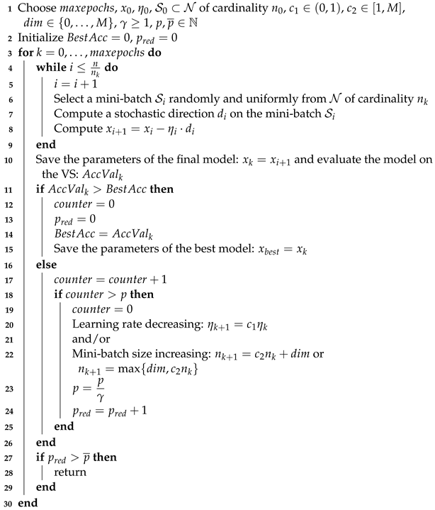
The complete scheme is described in Algorithm 1. The main features are reported below.
3.1.1. Lines 4–9—Update of the Iterates for One Epoch
The iterates are updated by means of a stochastic gradient algorithm (Algorithm 1 line 8) for an entire epoch. In particular, a stochastic estimate of the gradient of the objective function is computed by means of the current mini-batch of cardinality chosen randomly and uniformly from (lines 6–7). Examples of the stochastic gradient estimations are provided in (2) and (3).
3.1.2. Line 10—Evaluation of the Model
The model is evaluated on the VS, namely the accuracy is computed on the VS and saved in the variable .
3.1.3. Lines 11–15—Check for Accuracy Improvement
The current accuracy computed on the VS is compared to the one computed at the previous epoch and saved in the variable .
3.1.4. Lines 17–29—Dynamic Early Stopping
If the accuracy on the VS is not improved, a counter is increased (line 17). Subsequently (line 18), the value of the counter is compared to the prefixed value p of the patience. In standard early stopping strategies, if the counter is greater than the value of p, then the training phase is stopped. On the contrary, in the suggested dynamic early stopping technique, the training phase is not immediately stopped, but it is allowed to continue with different hyperparameters. In particular, the LR is decreased by a factor (line 20) and/or the MBS is increased by a proper rule (line 22) depending on and , where M is a constant related to hardware or memory limitations, for example, it can be the maximum number of samples which can be stored in the GPU. Finally (line 23), the value of the patience is divided by a factor . Thanks to a smaller LR and/or a mini-batch of a larger size, the optimizer employed in the training phase should stabilize and provide new iterates closer to the minimum point. However, if the LR becomes too small and the MBS reaches the hardware limitations, then the ending of the training process is forced. In particular, if the patience is reduced more than a prefixed value , then the training is stopped (lines 27–29).
To summarize, different from the standard early stopping, the proposed one avoids a sharp ending of the training process and the difficult tuning of a fixed value of the patience. Moreover, it allows to really exploit the nature of the dynamic selection rules for the LR and MBS, thus ensuring a more efficient learning phase. Finally, we remark that the possibility to refine the values for the LR and the MBS along the iterative process allows to make their initial setting less crucial than in the static approaches where the hyperparameters are kept fixed during the training.
| Algorithm 1: A stochastic gradient method with dynamical early stopping |
 |
4. Numerical Experiments
In this section, we investigate the effectiveness of the developed early stopping procedure combined with the SG method with momentum on image classification problems. More in detail, we consider Algorithm 1 where the stochastic direction (line 7) and the update of the iterates (line 8) are performed by means of the scheme defined in (3) with . The loss function in (1) is the cross entropy; hence, where is the probability of the Softmax function of the class i and is the true label. We consider both a standard database for image classification tasks as the CIFAR-100 [22] and two different biomedical databases of 2D images obtained by computed tomography tools [23,24,25,26,27].
4.1. Image Classification on CIFAR-100 Dataset
We present the results for three different CNNs for 100-classes classification on the CIFAR-100 dataset: ResNet18 [28], VGG16 [29] and MobileNet [30]. The numerical experiments have been performed on an Intel i9-9900KF coupled with an NVIDIA RTX 2080Ti. The code has been developed starting from an established framework to train several CNNs on the CIFAR-100 dataset (https://github.com/weiaicunzai/pytorch-cifar100, accessed on 1 October 2022) and has been made public for the sake of reproducibility (https://github.com/mive93/pytorch-cifar100, accessed on 1 October 2022). In the considered framework, the CIFAR-100 dataset was divided into training and test sets. We used 10% of the training set to create the validation set. The optimizer employed for the reference training of the CNNs is the SG with momentum; it uses a starting LR of 0.1 and schedules its annealing at epochs [60, 120, 160], multiplying it by 0.2 in those so-called milestones.
The performance of the optimization method employed for the CNNs reference training has been compared with the performance of two different versions of Algorithm 1 (with an SG with momentum at lines 7–8). In particular, we consider the possibility of either reducing the LR while the MBS is such that or decreasing the LR and increasing the MBS. Both versions of Algorithm 1 have been implemented by setting , , , , , where is the maximum number of samples that can be stored in the GPU, and . Moreover, in order to understand how the patience values affect the performance, we consider three different values for p—8, 15 and 20—and two different values for —2 and 4. Finally, has been fixed either equal to 6 if both the LR is reduced and the MBS is increased or equal to 3 if only the LR is decreased but the MBS is not changed along the iterations. In the results, the name of the different considered algorithms for the training reports:
- LR if only the LR is changed along the iterative process or LRBS if both the hyperparameters are variable;
- p followed by its value;
- followed by its value.
For example, LRBS_p20_2 points out that the selection rules for the LR and the MBS are both dynamic and the values for p and are 20 and 2, respectively.
All the tests have been performed five times, and the average accuracy on the test set and the number of epochs are reported, knowing that the standard deviation on the accuracy is at most equal to 0.0145. As usual, the best result obtained with the check on the VS is verified on the test set.
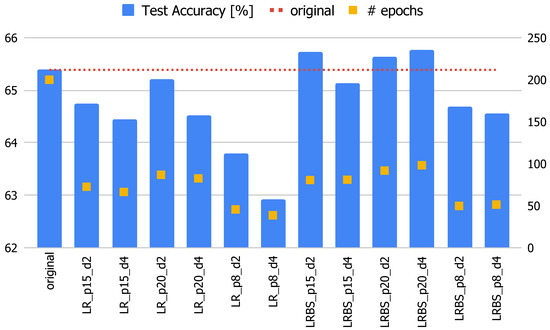
Figure 1 shows the results of all the experiments carried out on the MobileNet CNN. In this case, the reference training achieves an accuracy of 65.39% in 200 epochs. From the chart, it can be seen that all the trainings that follow the methodology proposed in this paper achieve similar results in terms of accuracy while needing less than half the epochs of the original one. Moreover, some configurations outperform the original, such as, e.g., the LRBS version with patience equal to 15 or 20. Table 1 reports all the results for the three CNNs for the LRBS configurations. From the last two columns of Table 1, it is possible to conclude that the accuracy results obtained by the proposed method are in line with those of the original version, sometimes slightly lower and sometimes higher. What is truly remarkable is the number of epochs required to obtain such a performance, which is at least halved compared to the original method.
Figure 1.
Performance of the various training for MobileNet on CIFAR-100. The blue bars represent the accuracy on the test set (left axis), the yellow squares report the number of epochs needed (right axis) and the red dotted line is the accuracy provided by the reference training.
Table 1.
Results obtained on the three CNN models on the CIFAR-100 dataset.
4.2. Biomedical Image Classification
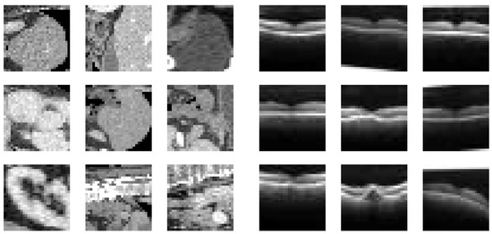
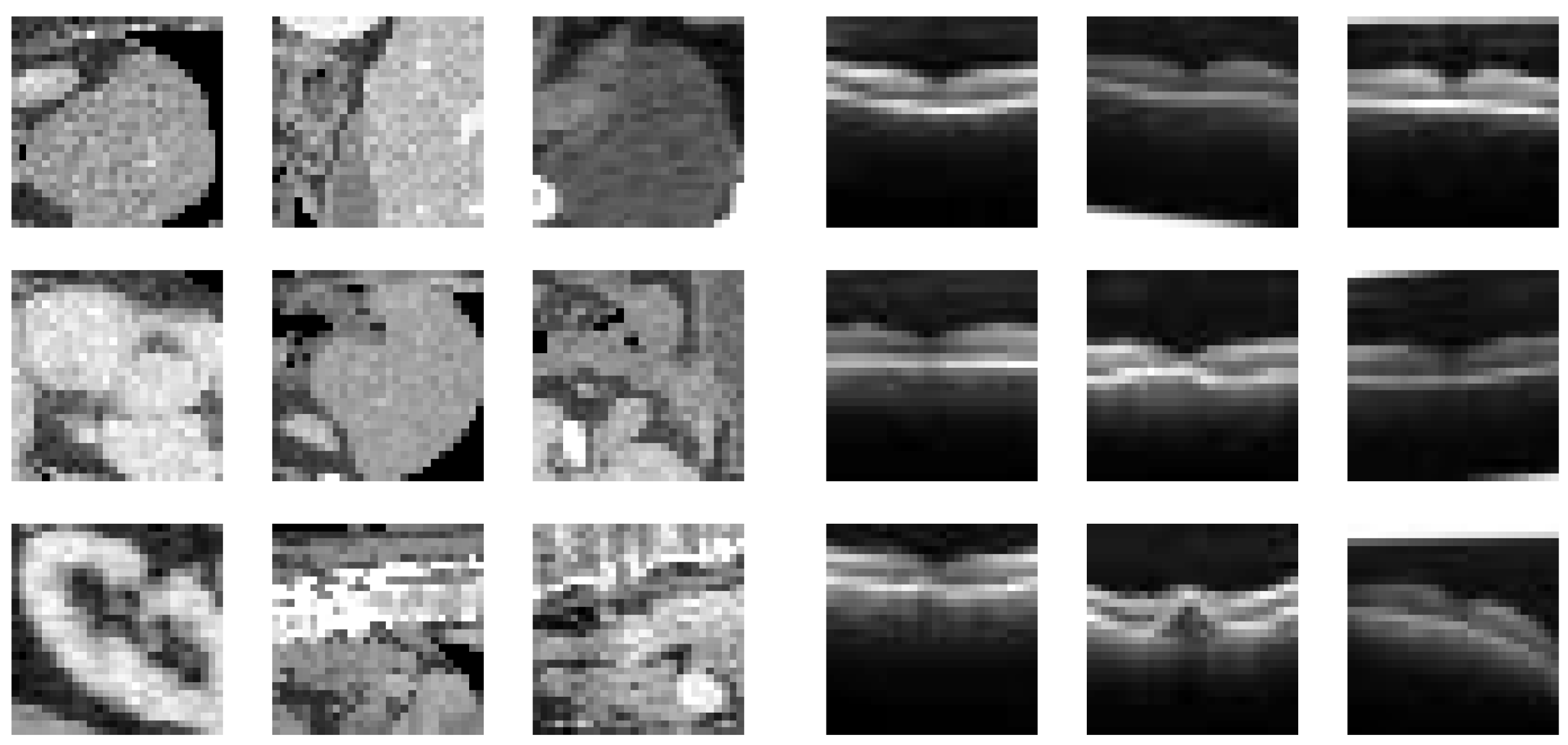
The second part of the numerical experiments involved two types of bidimensional biomedical image datasets for multi-class classification: MedMNIST2D OrganSMNIST (https://medmnist.com/, accessed on 1 October 2022) and MedMNIST OCTMNIST (https://medmnist.com/, accessed on 1 October 2022) [26,27]. The former is composed of 25,221 abdominal CT images (the first panel of Figure 2) with labels from 0 to 10, each one corresponding to an organ or a bone of the abdomen. Each image is 28 × 28 pixels and the original dataset is split up into training, validation and test sets whose dimensions correspond to 70%, 9% and 21% of the total number of samples, respectively. The second one is made up of 109309 optical coherence tomography (OCT) images for retinal diseases (the second panel of Figure 2) and there are four labels of which three correspond to different diseases and one is related to normal health conditions. Each image is 28 × 28 pixels and the original dataset is divided similarly to the previous case.
Figure 2.
Some examples from MedMNIST2D OrganSMNIST (left half) and OCTMNIST (right half).
These two applications have been processed on MSI Sword 15 A11UC-630XIT with a GPU NVIDIA GeForce RTX 3050 Laptop, CPU i7-11800H, 8 GB of RAM, Windows 11 and Python 3.10.2. We opportunely modified the official code (https://github.com/MedMNIST/MedMNIST, accessed on 1 October 2022) which implements various artificial neural networks, from the data splitting point of view. In particular, we divided the dataset into the following disjointed subsets: the 70% of the total examples gives the TS, the 9% is employed for the VS and the remaining 21% of the data forms the test set. Our code is publicly available (https://github.com/AmbraCatozzi/ResNet18_Biomedical.git, accessed on 1 October 2022) for the sake of reproducibility.
For all the experiments, we compared the performance of the ResNet18 model trained by means of:
- The SG optimizer (3) with (hereafter denoted by Original);
- The same optimizer but equipped with a classical early stopping technique (hereafter denoted by ES);
- Algorithm 1 (hereafter denoted by LRBS).
The hyperparameters setting for all the three optimization techniques are discussed in the following section.
4.2.1. Hyperparameters Setting
Because the performance of a stochastic gradient method is strictly related to the configuration of its hyperparameters, this section aims to fix the best hyperparameters setting for the algorithms employed to train the ResNet18. This preliminary study is carried out on the MedMNIST2D OrganSMNIST dataset and the best found hyperparameters configurations will be used for all the other experiments.
Setting p for the ES Method
First of all, we compare the performance of the ES method for different values of the patience p. In particular, given and , we report in Table 2 the values of the accuracy reached by ES with p equal to 5, 20 and 30. In the same table, the results corresponding to the Original optimizer are also reported (for the same setting of and ).
Table 2.
Results on MedMNIST2D OrganSMNIST dataset in a maximum of 50 epochs. is the standard deviation and each result is the mean of five trials.
The value of p, which ensures the best accuracy on the test set, is 20. In the following, p is always set to this value for the ES method.
Setting and for the Original and the ES Methods
In order to properly tune the LR and the MBS for both the Original and the ES schemes, we performed several experiments with different settings, illustrated in Table 3.
Table 3.
Hyperparameters analysis on MedMNIST2D OrganSMNIST dataset in a maximum of 50 epochs. is the standard deviation and each result is the mean of five trials.
From the results of Table 3, the best hyperparameters setting for both the Original and the ES approaches is and . We remark that to find this setting was very demanding in terms of computational costs.
Robustness of the LRBS Method against Hyperparameters
The proposed method aims to get rid of the dependence on its intrinsic hyperparameters while maintaining a high performance. In this section, we investigate the response of the LRBS method to the variation in the values of the hyperparameters used in Algorithm 1. In particular, we consider different values for: and . It is worth highlighting that we do not need to also properly tune the values for the patience, the LR and the MBS as performed for the Original and the ES schemes. Indeed, the LRBS algorithm automatically adjusts the values of these hyperparameters along the epochs. For this reason, we just consider , and : we select a quite large value for both the patience and the initial LR and a quite small value for the initial MBS by allowing the procedure to adapt them (by increasing the former ones and decreasing the latter one). To confirm this thesis, in the next section (see Table 7), we show that the LRBS algorithm is much less sensitive to the selection of the hyperparameters than the other two methods in training the ResNet18 for the MedMNIST2D OrganSMNIST dataset. In Table 4, we present the values of the accuracy for different configurations. We run each experiment five times with different seeds and we report the means and standard deviations in the table.
Table 4.
Mean and std. of the values of the accuracy obtained on MedMNIST2D OrganSMNIST dataset by the LRBS approach in a maximum of 50 epochs and different values of the hyperparameters. The initial mini-batch size is and the initial learning rate is .
Table 4 allows to conclude that the LRBS method is very stable with respect to the reasonable choices of the hyperparameters involved; particularly, both the mean and variance over the 5 trials are very good in all cases.
A Comparison with the AdaM Optimizer
Finally, for the sake of completeness, we show that to employ the AdaM optimizer [31], instead of the SG one with momentum, leads to analogous results. Table 5 reports the values of the accuracy reached by the considered approaches equipped by AdaM with and . The value of p is 20 for both the ES and LRBS. The LRBS method improves the accuracy obtained with the Original ResNet18 by one percentage point, with the lowest number of epochs.
Table 5.
Results on MedMNIST2D OrganSMNIST dataset in a maximum number of 50 epochs. The AdaM optimizer is employed with and .
4.2.2. Numerical Results
In this section, we perform three different experiments. We firstly summarize the hyperparameters setting for the three compared approaches in view of the considerations made in the previous section. For the Original, ES and LRBS, we fixed and . The value of p is 20 for both the ES and LRBS. Moreover, the other hyperparameters defining the LRBS are set as , , , , and . In the following paragraphs, we present the results obtained by fixing the maximum number of epochs, , to both 50 and 100.
Results for OrganSMNIST in a Maximum Number of 50 Epochs
In Table 6, we show the numerical results for the abdominal CT dataset: each column reports the mean accuracy on the test set, the standard deviation and the mean number of epochs obtained in five runs for the OrganSMNIST. The proposed method outperforms both the ResNet18 model and the early stopped one in terms of accuracy with the same number of epochs needed by the classical early stopping implementation.
Table 6.
Results on MedMNIST2D OrganSMNIST dataset in maximum 50 epochs.
We also observed that if we left fixed the value for the MBS but we increase the initial learning rate by either one or two orders of magnitude, the LRBS method outperforms both the standard model and the early stopped version (see Table 7) by confirming the less dependence on the hyperparameters setting of the LRBS approach.
Table 7.
Results on MedMNIST2D OrganSMNIST dataset in a maximum of 50 epochs.
Results for OCTMNIST Dataset in a Maximum Number of 50 Epochs
The results related to the MedMNIST2D OCTMNIST dataset are illustrated in the same vein, but the means are calculated on the best five values of each configuration chosen from 20 runs; the numerical outcomes are presented in Table 8. It can be seen that the proposed method slightly improves the accuracy, but it reaches this value in half of the time with respect to the standard early stopping procedure.
Table 8.
Results on MedMNIST2D OCTMNIST dataset in maximum 50 epochs.
Results for OCTMNIST in a Maximum Number of 100 Epochs
To highlight the effectiveness of Algorithm 1, another experiment has been conducted. We trained the same models presented in the previous section for a maximum number of 100 epochs by considering the dataset OCTMNIST (see Table 9).
Table 9.
Results on MedMNIST2D OCTMNIST dataset in maximum 100 epochs.
As in the previous experiments, comparable values for the accuracy can be obtained by all the considered strategies; however, the number of epochs related to the early stopped models is less than the 20% of the total number of epochs. However, we remark that the LRBS does not suffer from the computational expensive phase of the hyperparameters tuning.
5. Conclusions and Future Works
In this paper, we propose a dynamic early stopping technique for the training of a neural network, based on variable selection strategies to fix both the learning rate and the mini-batch size in SG methods. The suggested scheme is able to avoid the overfitting phenomena and reduce the training phase. The numerical experiments carried out on biomedical image classification problems show the benefits of employing the proposed dynamic early stopping procedure: performances comparable to those of the reference network can be achieved in a significantly lower number of epochs. Moreover, the suggested approach avoids the computational expensive setting of the best hyperparameters values needed by standard training techniques.
Author Contributions
All authors contributed equally to the study conception and design. Data curation, M.V.; software, A.C.; supervision, M.P.; validation, F.P.; writing—original draft, G.F. All authors have read and agreed to the published version of the manuscript.
Funding
This research received no external funding.
Institutional Review Board Statement
Not applicable.
Informed Consent Statement
Not applicable.
Data Availability Statement
https://github.com/weiaicunzai/pytorch-cifar100 (accessed on 1 October 2022), https://github.com/mive93/pytorch-cifar100 (accessed on 1 October 2022).
Acknowledgments
This work was also supported by the Gruppo Nazionale per il Calcolo Scientifico (GNCS-INdAM). The publication was created with the co-financing of the European Union-FSE-REACT-EU, PON Research and Innovation 2014-2020 DM1062/2021. The publication is co-financed by the project Unimore FAR Mission Oriented “Artificial Intelligence-based Mathematical Models and Methods for low dose CT imaging”.
Conflicts of Interest
The authors declare no conflict of interest.
Abbreviations
The following abbreviations are used in this manuscript:
| AI | Artificial Intelligence |
| ML | Machine Learning |
| DL | Deep Learning |
| SG | Stochastic Gradient |
| MBS | Mini-Batch Size |
| NAS | Neural Architecture Search |
| LR | Learning Rate |
| VS | Validation Set |
| ANN | Artificial Neural Network |
| GPU | Graphics Processing Unit |
| FPGA | Field-Programmable Gate Array |
| CNN | Convolutional Neural Network |
| TS | Training Set |
References
- Bottou, L.; Curtis, F.; Nocedal, J. Optimization Methods for Large-Scale Machine Learning. SIAM Rev. 2018, 60, 223–311. [Google Scholar] [CrossRef] [Scilit]
- Loizou, N.; Richtárik, P. Momentum and Stochastic Momentum for Stochastic Gradient, Newton, Proximal Point and Subspace Descent Methods. Comput. Optim. Appl. 2020, 77, 653–710. [Google Scholar] [CrossRef] [Scilit]
- Franchini, G.; Ruggiero, V.; Porta, F.; Zanni, L. Neural architecture search via standard machine learning methodologies. Math. Eng. 2022, 5, 1–21. [Google Scholar] [CrossRef] [Scilit]
- Nakkiran, P. Learning Rate Annealing Can Provably Help Generalization, Even for Convex Problems. In Proceedings of the OPT2020: 12th Annual Workshop on Optimization for Machine Learning, Bangkok, Thailand, 18–20 November 2020; p. 35. [Google Scholar]
- Li, Y.; Wei, C.; Ma, T. Towards Explaining the Regularization Effect of Initial Large Learning Rate in Training Neural Networks. In Proceedings of the 33rd International Conference on Neural Information Processing Systems, Vancouver, BC, Canada, 8–14 November 2019; Curran Associates Inc.: Red Hook, NY, USA, 2019; p. 1047. [Google Scholar]
- Bochkovskiy, A.; Wang, C.; Liao, H.M. YOLOv4: Optimal Speed and Accuracy of Object Detection. arXiv 2020, arXiv:abs/2004.10934. [Google Scholar]
- Ramachandran, S.; George, J.; Skaria, S.; Varun, V. Using YOLO based deep learning network for real time detection and localization of lung nodules from low dose CT scans. In Proceedings of the Medical Imaging 2018: Computer-Aided Diagnosis, Houston, TX, USA, 12–15 February 2018; Volume 10575, p. 105751I. [Google Scholar] [CrossRef] [Scilit]
- Takase, T.; Oyama, S.; Kurihara, M. Effective neural network training with adaptive learning rate based on training loss. Neural Netw. 2018, 101, 68–78. [Google Scholar] [CrossRef] [Scilit]
- Mishra, S.; Yamasaki, T.; Imaizumi, H. Improving image classifiers for small datasets by learning rate adaptations. In Proceedings of the 16th International Conference on Machine Vision Applications (MVA), Tokyo, Japan, 27–31 May 2019. [Google Scholar] [CrossRef] [Scilit]
- Masters, D.; Luschi, C. Revisiting Small Batch Training for Deep Neural Networks. arXiv 2018, arXiv:1804.07612. [Google Scholar]
- Friedlander, M.; Schmidt, M. Hybrid Deterministic-Stochastic Methods for Data Fitting. SIAM J. Sci. Comput. 2012, 34, A1380–A1405. [Google Scholar] [CrossRef] [Scilit]
- Alfarra, M.; Hanzely, S.; Albasyoni, A.; Ghanem, B.; Richtarik, P. Adaptive Learning of the Optimal Mini-Batch Size of SGD. In Proceedings of the OPT2020: 12th Annual Workshop on Optimization for Machine Learning, Bangkok, Thailand, 18–20 November 2020; p. 10. [Google Scholar]
- Franchini, G.; Burgio, P.; Zanni, L. Artificial Neural Networks: The Missing Link Between Curiosity and Accuracy. In Proceedings of the Intelligent Systems Design and Applications, Vellore, India, 12–15 December 2020; Abraham, A., Cherukuri, A., Melin, P., Gandhi, N., Eds.; Springer International Publishing: Cham, Switzerland, 2020; pp. 1025–1034. [Google Scholar]
- Kandel, I.; Castelli, M. The effect of batch size on the generalizability of the convolutional neural networks on a histopathology dataset. ICT Express 2020, 6, 312–315. [Google Scholar] [CrossRef] [Scilit]
- Smith, S.; Kindermans, P.J.; Le, Q. Don’t Decay the Learning Rate, Increase the Batch Size. In Proceedings of the 6th International Conference on Learning Representations, Vancouver, BC, Canada, 30 April–3 May 2018. [Google Scholar]
- Franchini, G.; Ruggiero, V.; Zanni, L. Steplength and Mini-batch Size Selection in Stochastic Gradient Methods. In Proceedings of the Machine Learning, Optimization, and Data Science, Siena, Italy, 19–23 July 2020; Nicosia, G., Ojha, V., La Malfa, E., Jansen, G., Sciacca, V., Pardalos, P., Giuffrida, G., Umeton, R., Eds.; Springer International Publishing: Berlin/Heidelberg, Germany, 2020; pp. 259–263. [Google Scholar]
- Chen, C.; Zhang, Y.; Wang, Z.; Wan, S.; Pei, Q. Distributed computation offloading method based on deep reinforcement learning in ICV. Appl. Soft Comput. 2021, 103, 107108. [Google Scholar] [CrossRef] [Scilit]
- Wu, Y.; Yue, Y.; Tan, X.; Wang, W.; Lu, T. End-to-end chromosome Karyotyping with data augmentation using GAN. In Proceedings of the 2018 25th IEEE International Conference on Image Processing (ICIP), Athens, Greece, 7–10 October 2018; pp. 2456–2460. [Google Scholar]
- Sun, L.; Feng, S.; Liu, J.; Lyu, G.; Lang, C. Global-local label correlation for partial multi-label learning. IEEE Trans. Multimed. 2021, 24, 581–593. [Google Scholar] [CrossRef] [Scilit]
- Prechelt, L. Early Stopping—But When? In Neural Networks: Tricks of the Trade, 2nd ed.; Montavon, G., Orr, G.B., Müller, K.R., Eds.; Springer: Berlin/Heidelberg, Germany, 2012; pp. 53–67. [Google Scholar]
- Schwartz, R.; Dodge, J.; Smith, N.; Etzioni, O. Green AI. Commun. ACM 2020, 63, 54–63. [Google Scholar] [CrossRef] [Scilit]
- Krizhevsky, A.; Hinton, G. Learning Multiple Layers of Features from Tiny Images; Technical Report TR-2009; University of Toronto: Toronto, ON, Canada, 2009. [Google Scholar]
- Yang, J.; Shi, R.; Wei, D.; Liu, Z.; Zhao, L.; Ke, B.; Pfister, H.; Ni, B. MedMNIST v2: A Large-Scale Lightweight Benchmark for 2D and 3D Biomedical Image Classification. arXiv 2021, arXiv:2110.14795. [Google Scholar]
- Kermany, D.; Goldbaum, M. Identifying Medical Diagnoses and Treatable Diseases by Image-Based Deep Learning. Cell 2018, 172, 1122–1131. [Google Scholar] [CrossRef] [Scilit]
- Yang, J.; Shi, R.; Ni, B. MedMNIST Classification Decathlon: A Lightweight AutoML Benchmark for Medical Image Analysis. In Proceedings of the IEEE 18th International Symposium on Biomedical Imaging (ISBI), Nice, France, 13–16 April 2021; pp. 191–195. [Google Scholar]
- Bilic, P.; Christ, P.F.; Vorontsov, E.; Chlebus, G.; Chen, H.; Dou, Q.; Menze, B.H. The Liver Tumor Segmentation Benchmark (LiTS). arXiv 2019, arXiv:1901.04056. [Google Scholar]
- Xu, X.; Zhou, F.; Liu, B.; Fu, D.; Bai, X. Efficient Multiple Organ Localization in CT Image Using 3D Region Proposal Network. IEEE Trans. Med. Imaging 2019, 38, 1885–1898. [Google Scholar] [CrossRef] [Scilit] [PubMed]
- He, K.; Zhang, X.; Ren, S.; Sun, J. Deep residual learning for image recognition. In Proceedings of the IEEE Conference on Computer Vision and Pattern Recognition, Las Vegas, NV, USA, 27–30 June 2016; pp. 770–778. [Google Scholar]
- Simonyan, K.; Zisserman, A. Very deep convolutional networks for large-scale image recognition. arXiv 2014, arXiv:1409.1556. [Google Scholar]
- Howard, A.G.; Zhu, M.; Chen, B.; Kalenichenko, D.; Wang, W.; Weyand, T.; Andreetto, M.; Adam, H. MobileNets: Efficient convolutional neural networks for mobile vision applications. arXiv 2017, arXiv:1704.04861. [Google Scholar]
- Kingma, D.; Ba, J. Adam: A Method for Stochastic Optimization. arXiv 2017, arXiv:1412.6980. [Google Scholar]

Publisher’s Note: MDPI stays neutral with regard to jurisdictional claims in published maps and institutional affiliations. |
© 2022 by the authors. Licensee MDPI, Basel, Switzerland. This article is an open access article distributed under the terms and conditions of the Creative Commons Attribution (CC BY) license (https://creativecommons.org/licenses/by/4.0/).