Author Contributions
Conceptualization, S.C., N.L., N.M. and M.T.; methodology, S.C., N.L., N.M. and M.T.; software N.M.; validation, S.C., N.L., N.M. and M.T.; formal analysis, S.C., N.L., N.M. and M.T.; investigation, S.C., N.L., N.M. and M.T.; resources, S.C., N.L., N.M. and M.T.; data curation N.L. and N.M.; writing—original draft preparation, N.M.; writing—review and editing, S.C., N.L., N.M. and M.T.; visualization, S.C., N.L., N.M. and M.T.; supervision, S.C., N.L. and M.T.; project administration, S.C., N.L. and M.T.; funding acquisition, S.C., N.L. All authors have read and agreed to the published version of the manuscript.
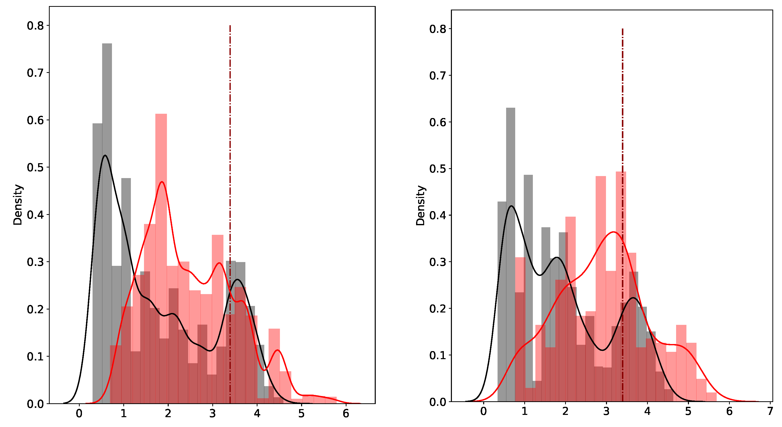
Figure 1.
Empirical densities of anomaly scores given by the naive approach for uncontaminated time series in black and contaminated time series in red in a training set (left) and test set (right). The dotted dark red lines represent the cutoff values.
Figure 1.
Empirical densities of anomaly scores given by the naive approach for uncontaminated time series in black and contaminated time series in red in a training set (left) and test set (right). The dotted dark red lines represent the cutoff values.
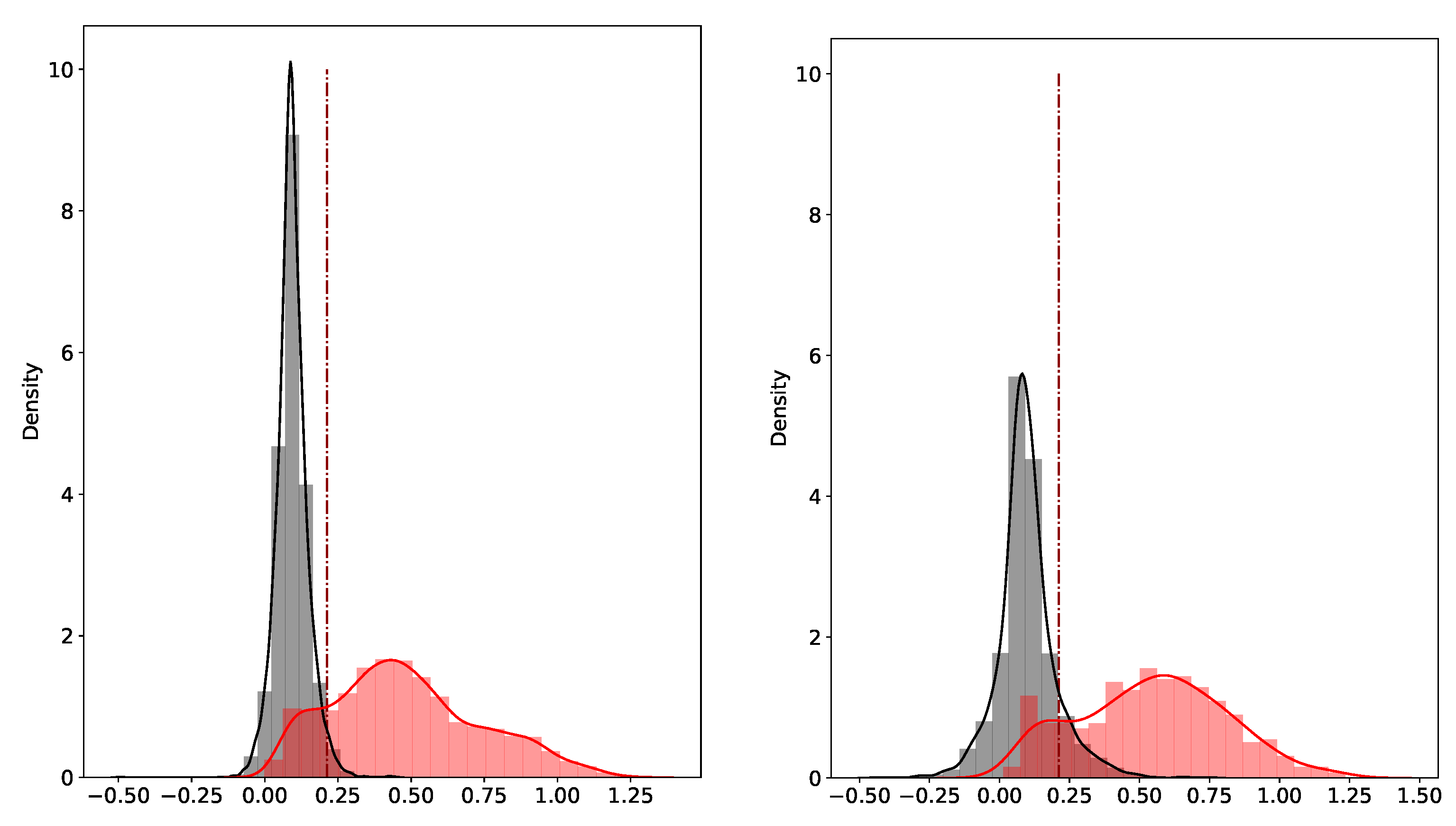
Figure 2.
Empirical densities of anomaly scores given by the NN approach for uncontaminated time series in black and contaminated time series in red for the training set (left) and test set (right). The dotted dark red lines represent the calibrated cutoff value .
Figure 2.
Empirical densities of anomaly scores given by the NN approach for uncontaminated time series in black and contaminated time series in red for the training set (left) and test set (right). The dotted dark red lines represent the calibrated cutoff value .
Figure 3.
Flow chart of our two-step anomaly detection model (PCA NN), depicting the process a time series X undergoes.
Figure 3.
Flow chart of our two-step anomaly detection model (PCA NN), depicting the process a time series X undergoes.
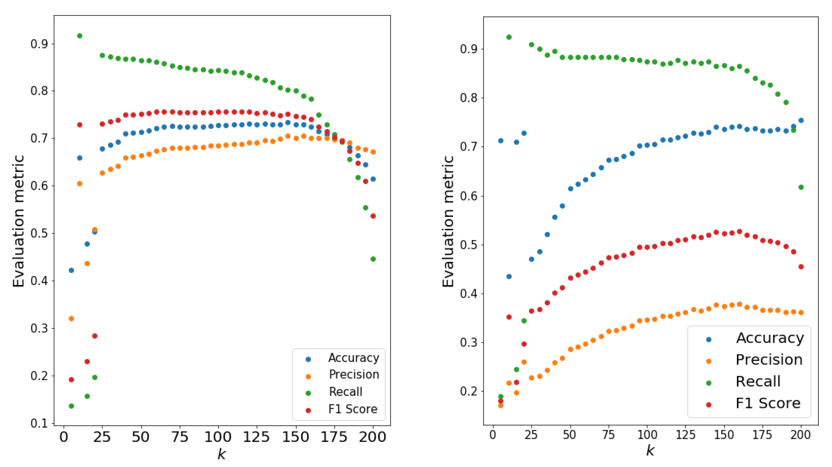
Figure 4.
Performance metrics for the training (left) and test (right) sets with respect to the number of principal components k.
Figure 4.
Performance metrics for the training (left) and test (right) sets with respect to the number of principal components k.
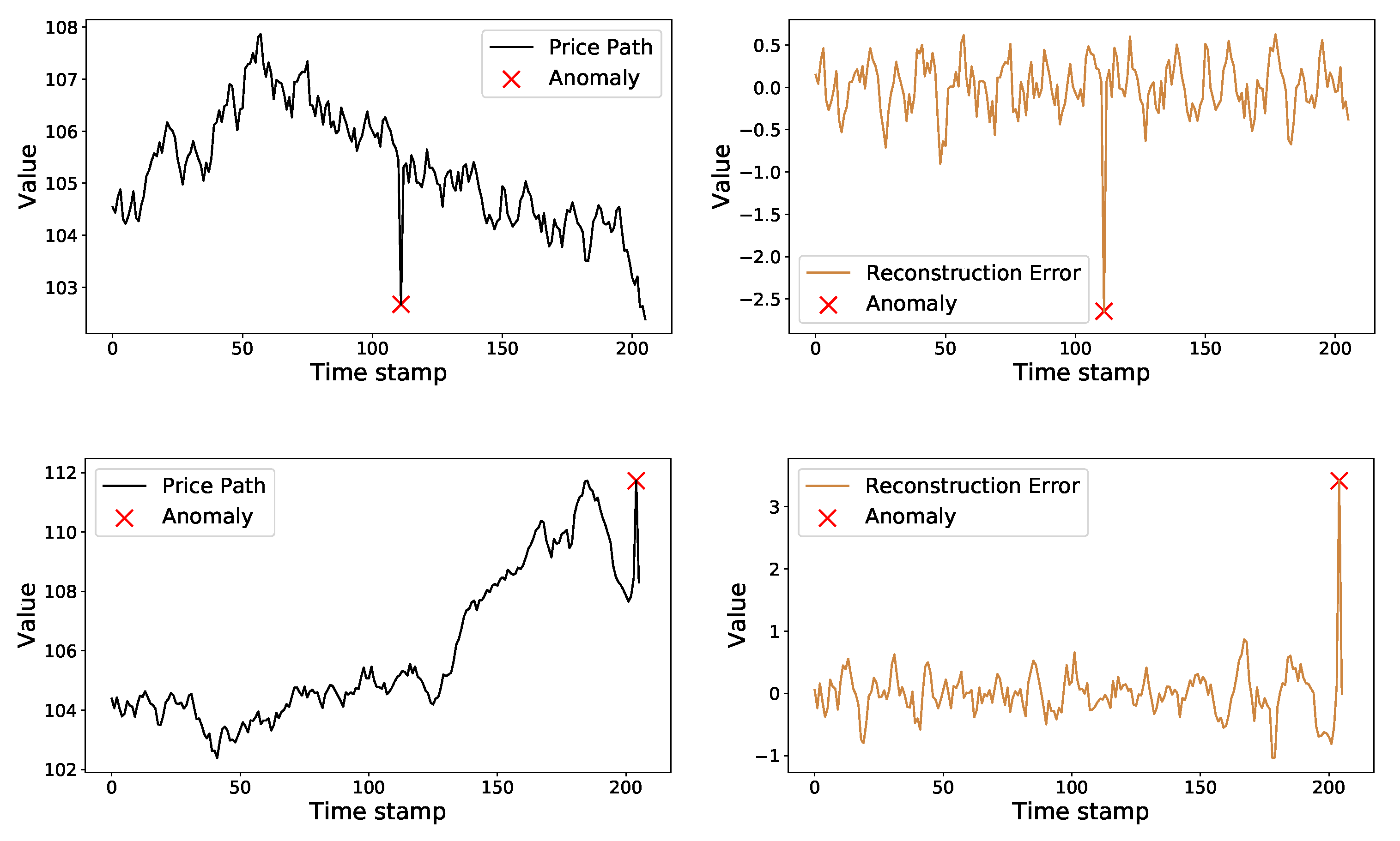
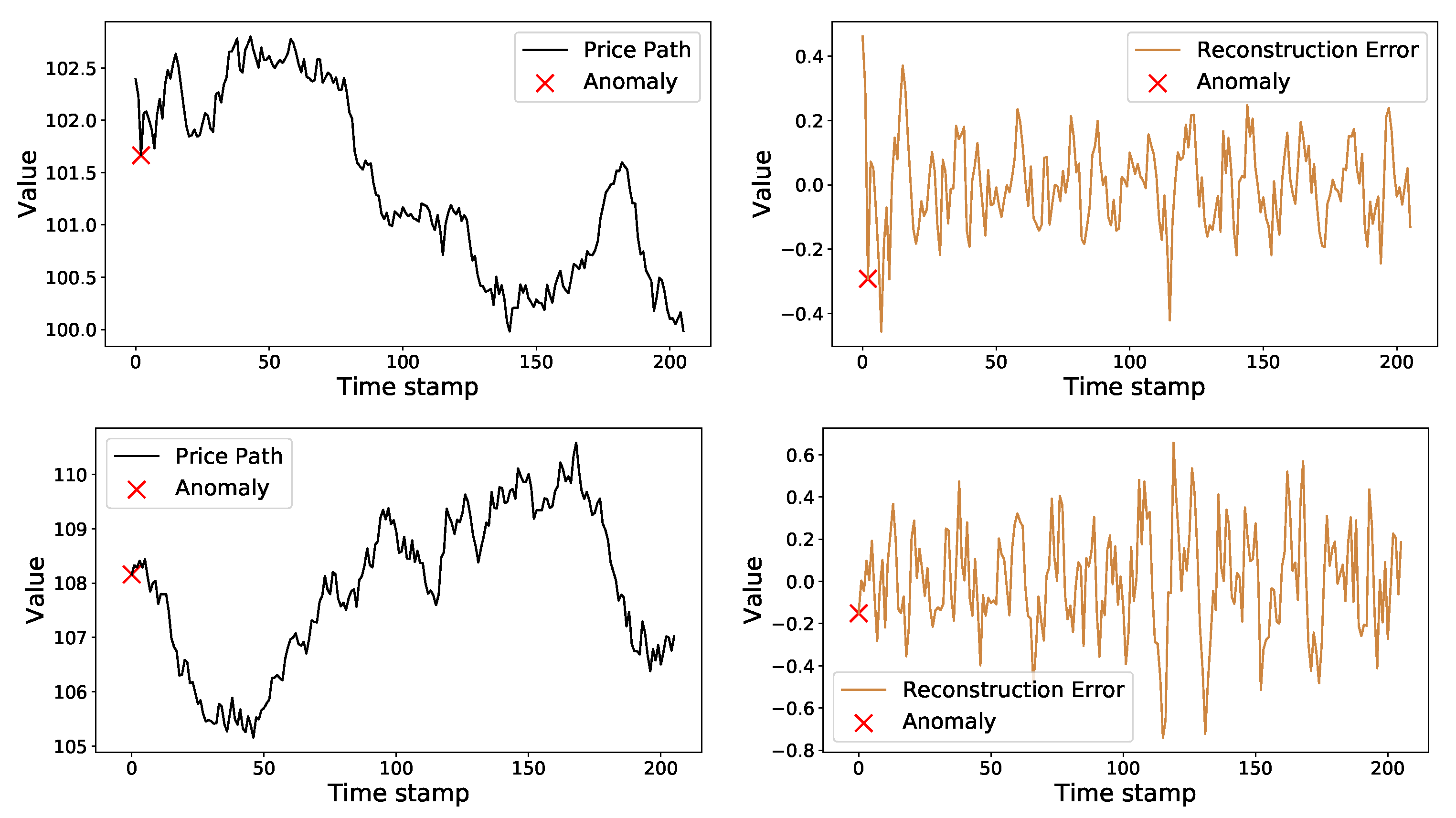
Figure 5.
Two examples of contaminated time series accurately identified by the model. The stock path and the reconstruction errors are represented in black and brown. The red cross shows the anomaly localization.
Figure 5.
Two examples of contaminated time series accurately identified by the model. The stock path and the reconstruction errors are represented in black and brown. The red cross shows the anomaly localization.
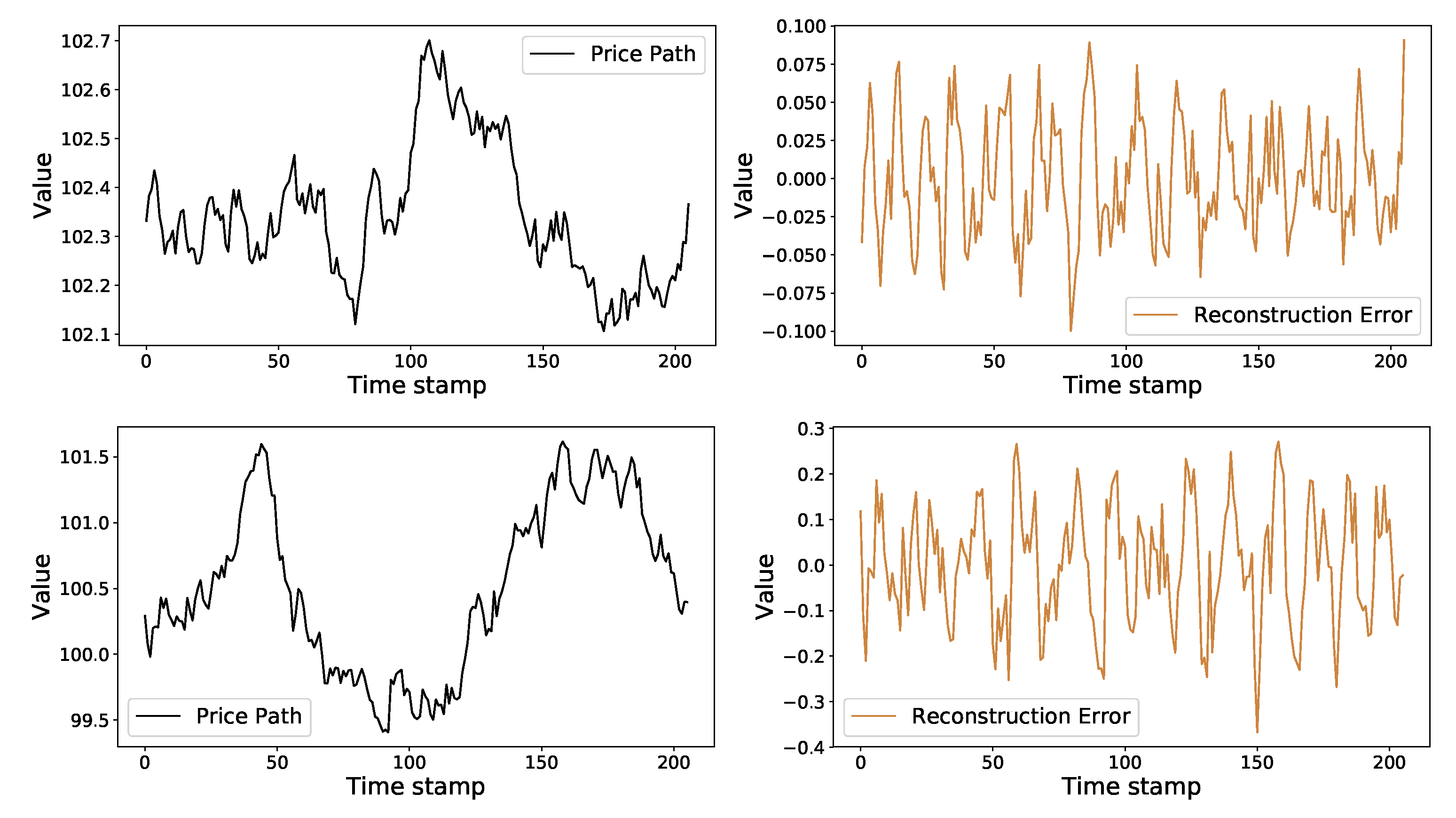
Figure 6.
Two examples of uncontaminated time series accurately identified by the model. The stock path and the reconstruction errors are represented in black and brown.
Figure 6.
Two examples of uncontaminated time series accurately identified by the model. The stock path and the reconstruction errors are represented in black and brown.
Figure 7.
Two examples of time series misidentified by the model. The stock path and the reconstruction errors are represented in black and brown. The red cross shows the anomaly localization.
Figure 7.
Two examples of time series misidentified by the model. The stock path and the reconstruction errors are represented in black and brown. The red cross shows the anomaly localization.
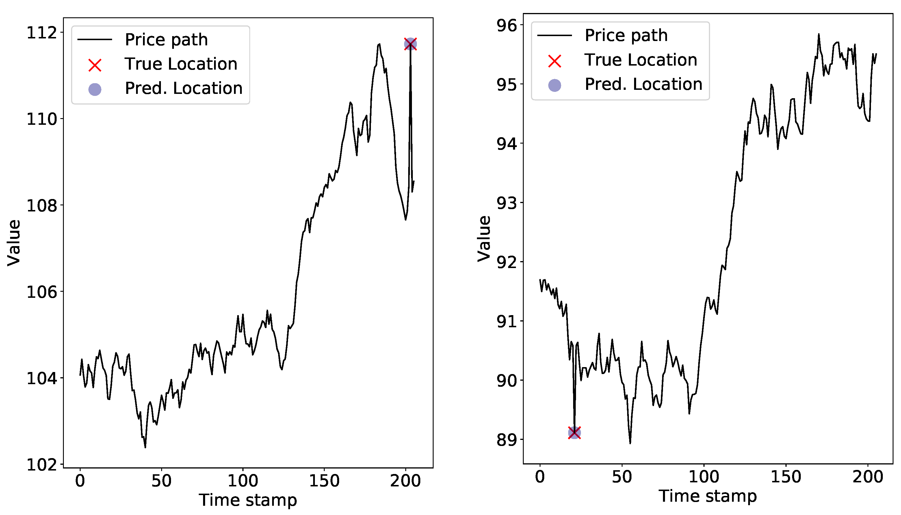
Figure 8.
Anomaly localization prediction for two distinct time series.
Figure 8.
Anomaly localization prediction for two distinct time series.
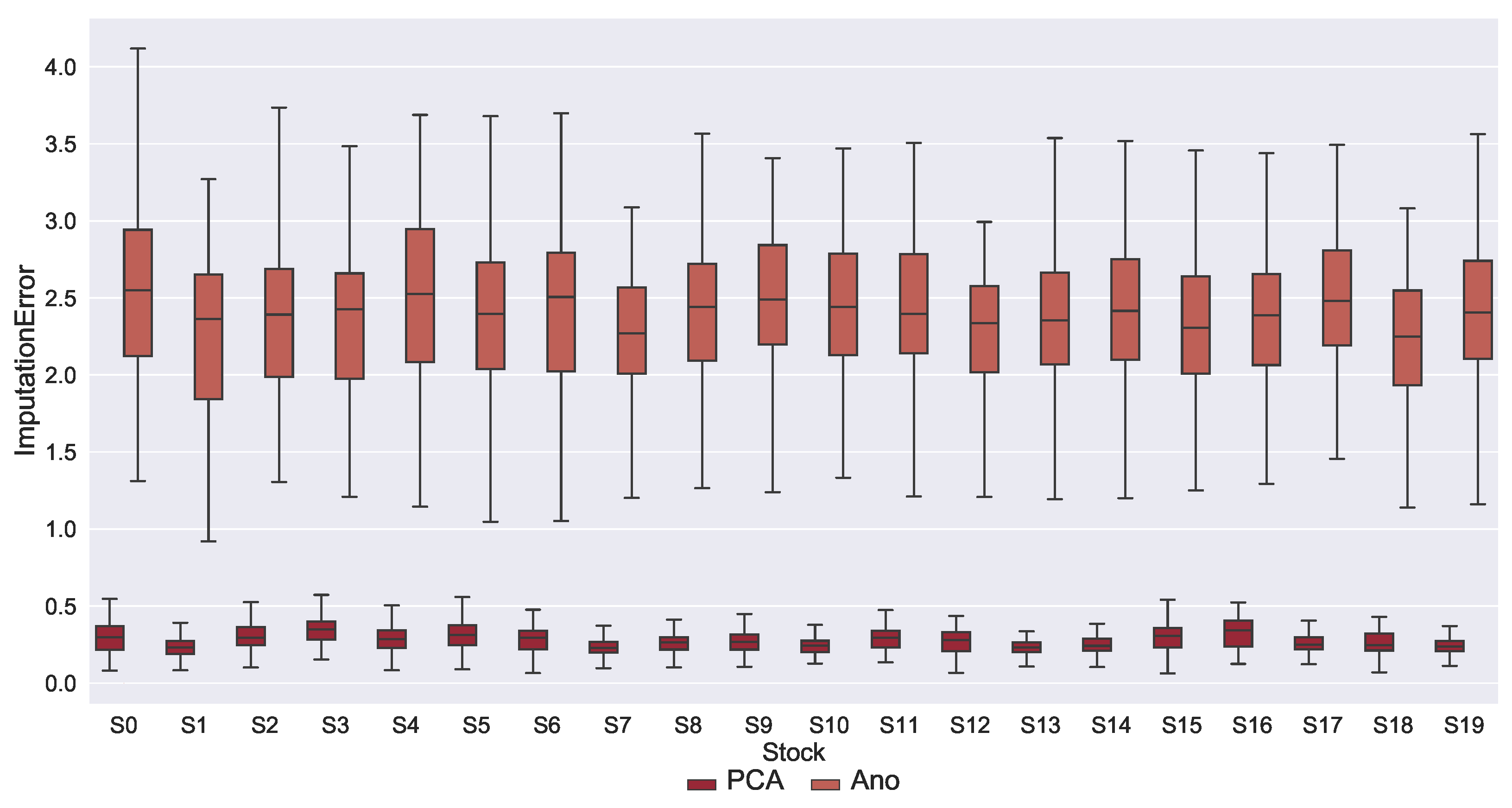
Figure 9.
Box plot representation of the distribution of the errors on the time series imputation before the imputation of anomalies (Ano) and after replacing the anomalies with the reconstructed values suggested by the PCA NN (PCA).
Figure 9.
Box plot representation of the distribution of the errors on the time series imputation before the imputation of anomalies (Ano) and after replacing the anomalies with the reconstructed values suggested by the PCA NN (PCA).
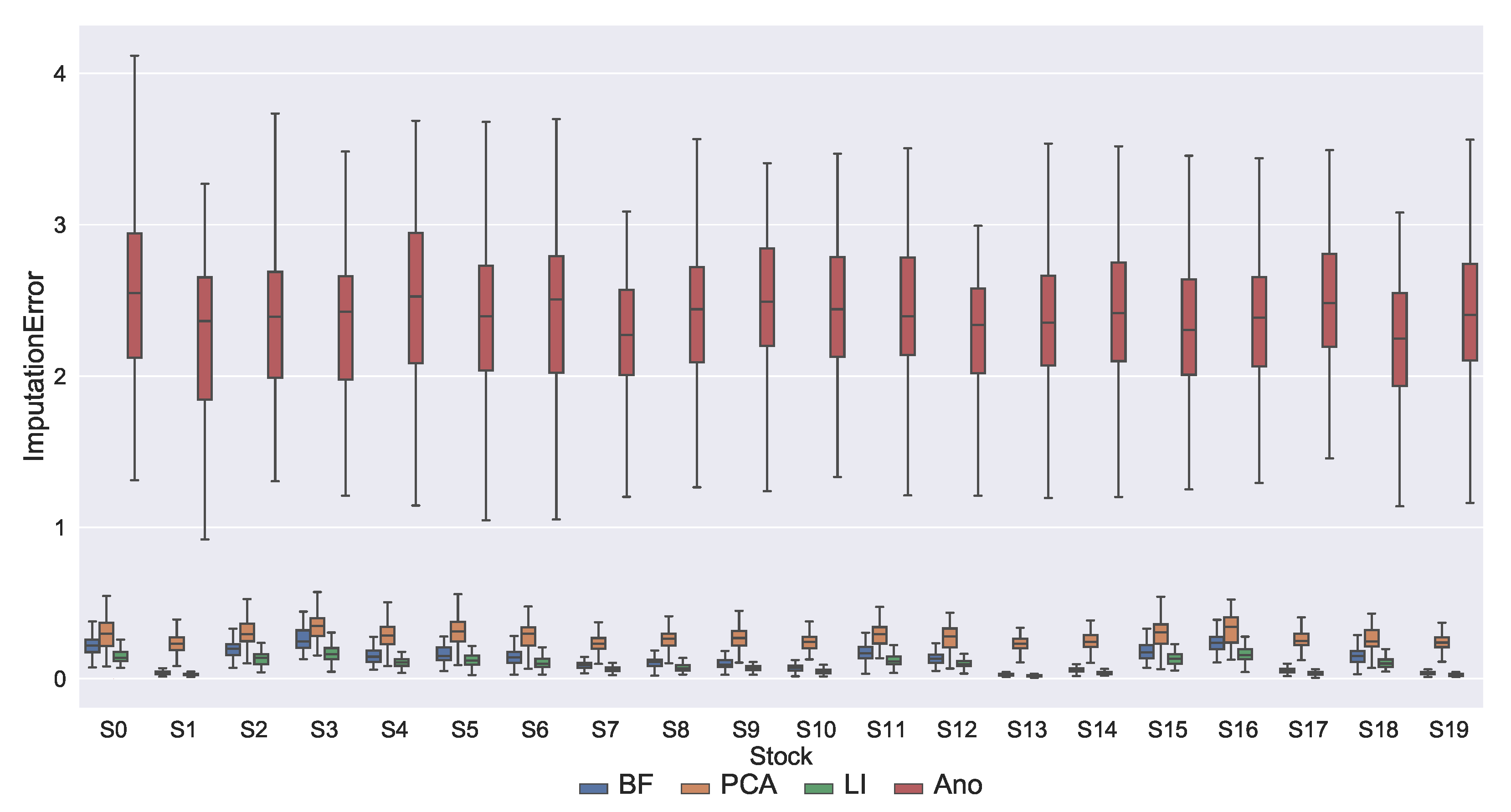
Figure 10.
Box plot representation of the distribution of the errors on the time series imputation before the imputation of anomalies (Ano) and after replacing the anomalies with the reconstructed values suggested by PCA using linear interpolation (LI) and backward fill (BF).
Figure 10.
Box plot representation of the distribution of the errors on the time series imputation before the imputation of anomalies (Ano) and after replacing the anomalies with the reconstructed values suggested by PCA using linear interpolation (LI) and backward fill (BF).
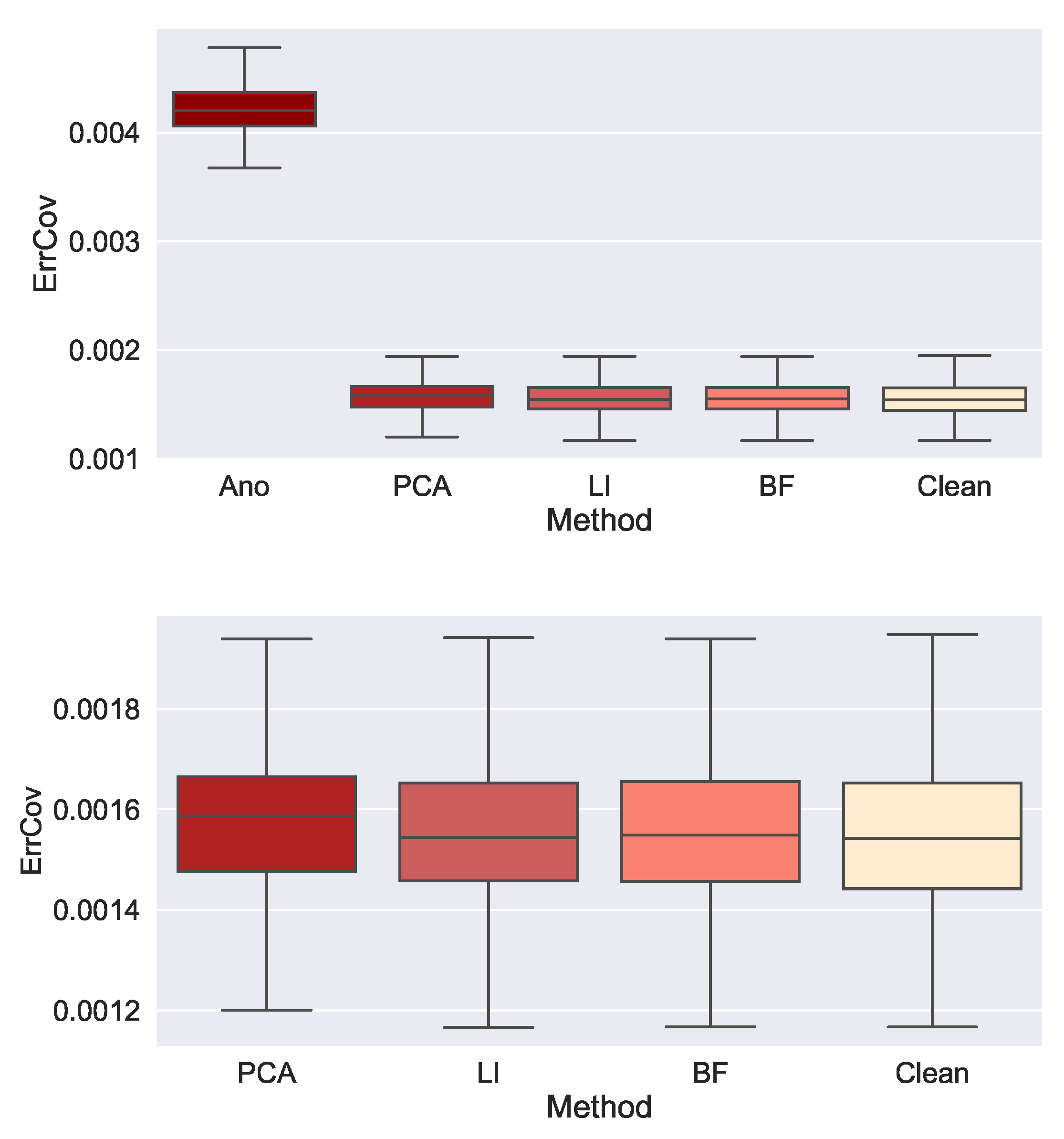
Figure 11.
Box plot representation of the distribution of the errors on the covariance matrix (on several stock path samples). Ano, PCA NN, LI, BF, and Clean refer to the errors in the covariance when estimated for time series with anomalies; time series after anomaly imputation following three approaches, imputation by the reconstructed values suggested by PCA, linear interpolation (LI), backward fill (BF); and time series without anomalies (Clean). The Ano, PCA NN, LI, BF, and Clean errors in the covariance estimation are all represented (upper). For better visualization we remove the Ano errors (below).
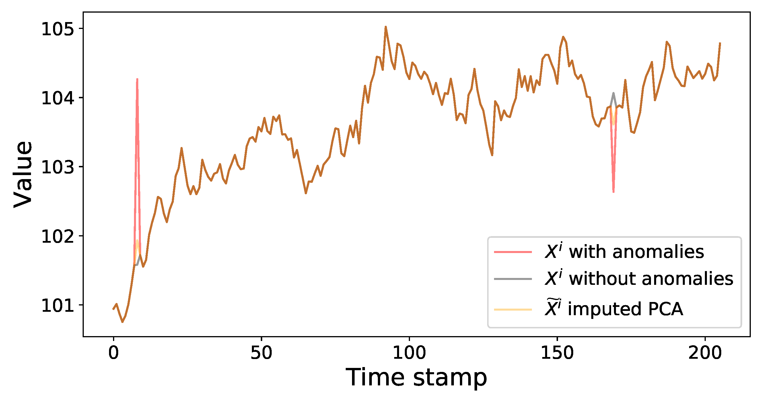
Figure 12.
Original, contaminated, and reconstructed stock price paths.
Figure 12.
Original, contaminated, and reconstructed stock price paths.
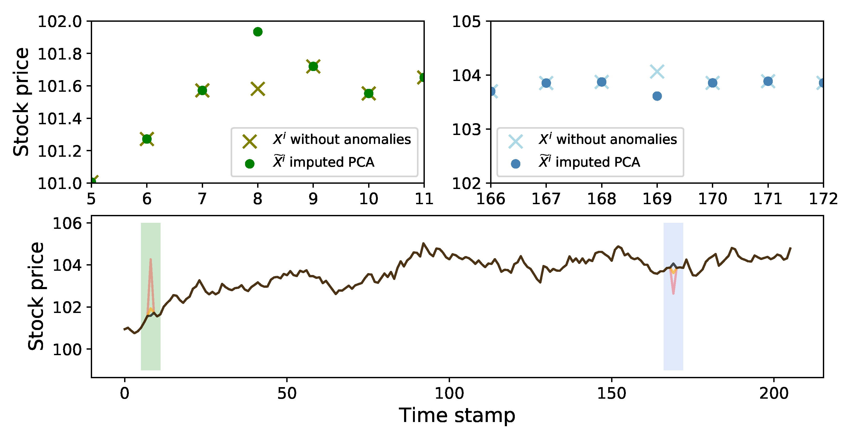
Figure 13.
Original, contaminated, and imputed stock price paths in black, red, and orange. The two additional graphs represent the region around the anomalies, where the crosses and circles, respectively, show the true value of the stock and its value after imputation of the anomalies using the reconstructed value suggested by the PCA NN approach.
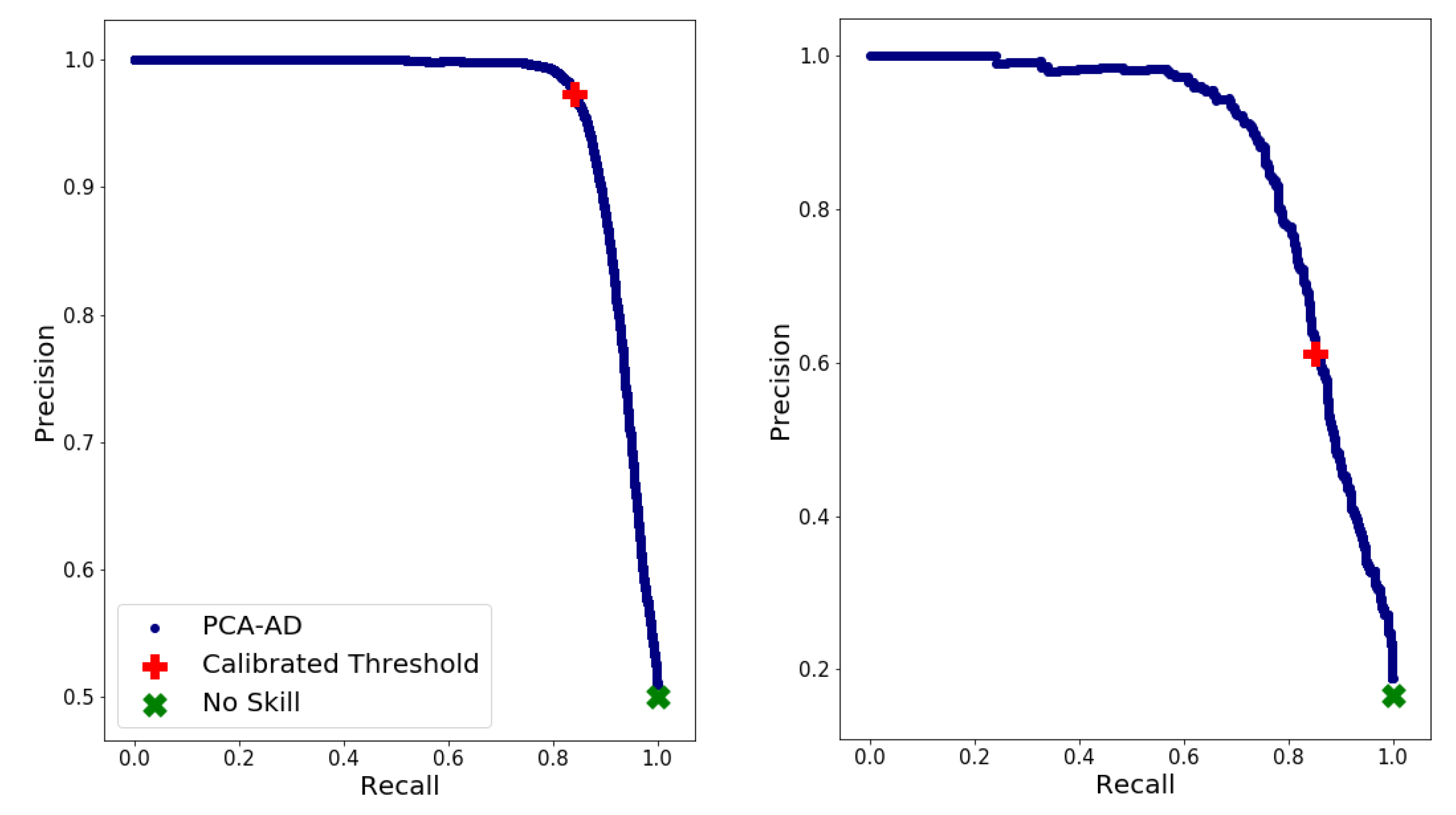
Figure 14.
Precision–recall curve of the suggested model (in blue), the scores for the calibrated threshold (red plus), the no-skill model scores (green cross) for the training (left) and test sets (right).
Figure 14.
Precision–recall curve of the suggested model (in blue), the scores for the calibrated threshold (red plus), the no-skill model scores (green cross) for the training (left) and test sets (right).
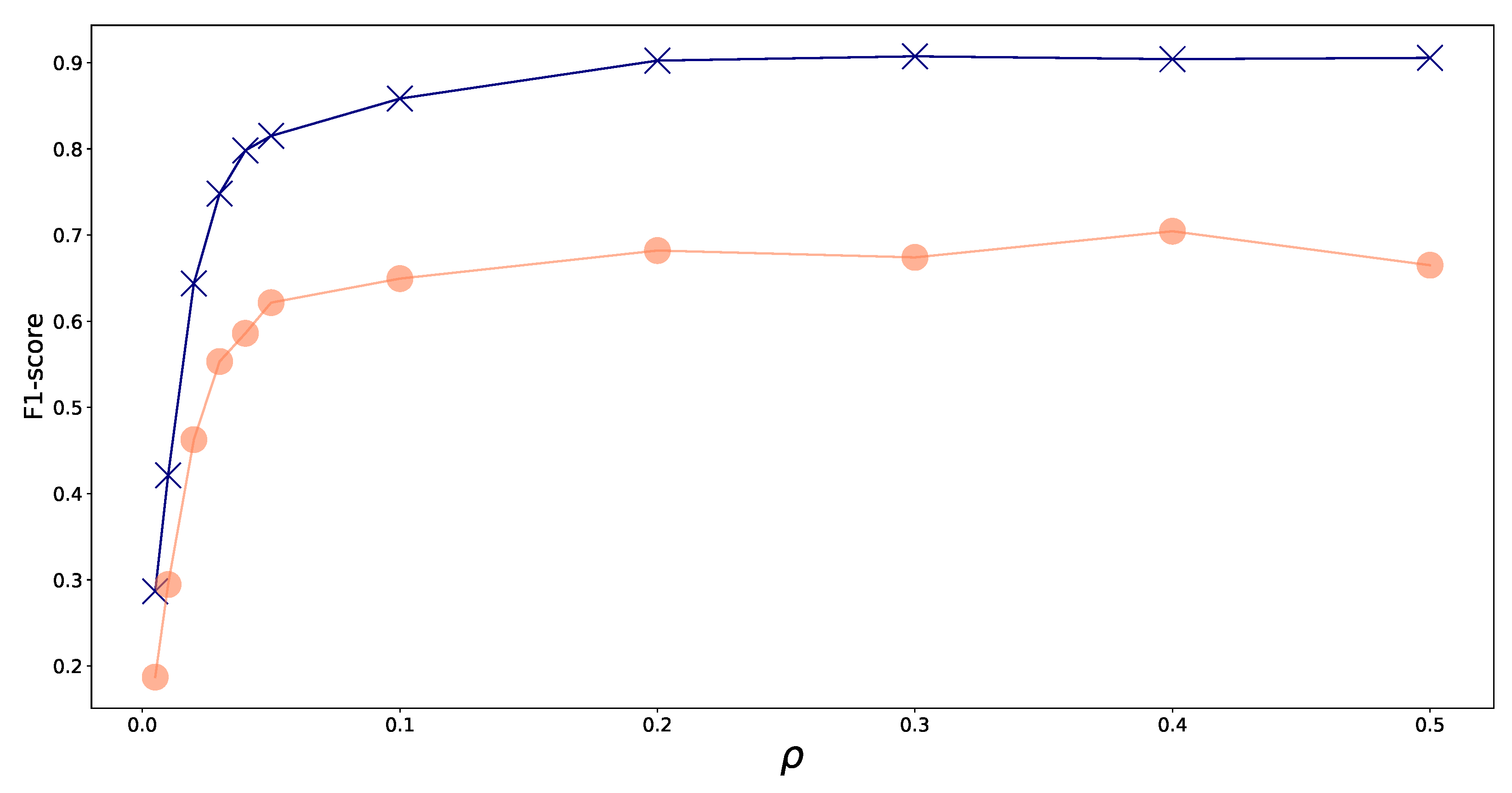
Figure 15.
Mean -score for identification step with respect to the various values of for the training and test sets, respectively, represented by the blue and pink curves.
Figure 15.
Mean -score for identification step with respect to the various values of for the training and test sets, respectively, represented by the blue and pink curves.
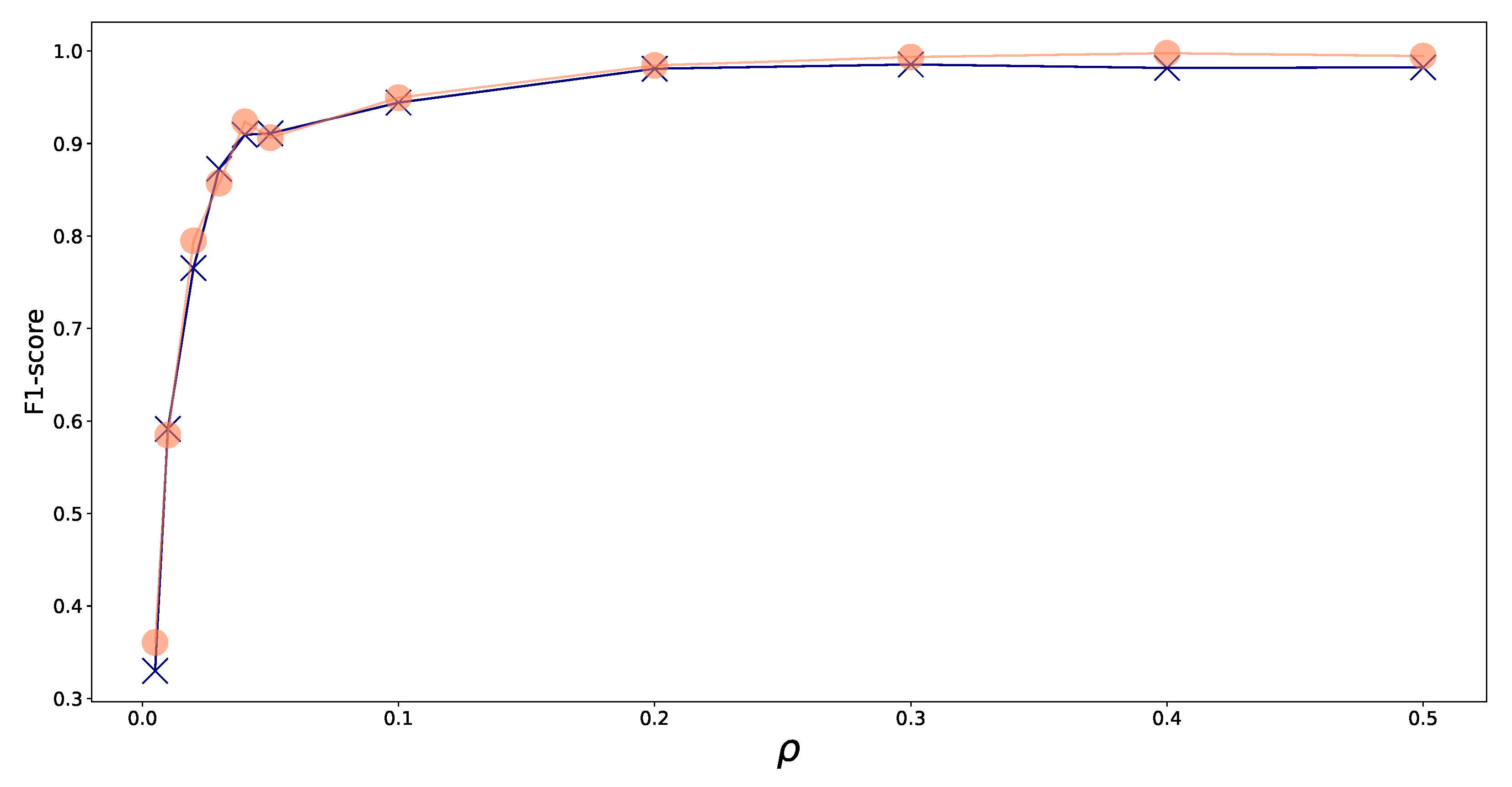
Figure 16.
Mean -score for localization step with respect to the various values of for the training and test sets, respectively, represented by the blue and pink curves.
Figure 16.
Mean -score for localization step with respect to the various values of for the training and test sets, respectively, represented by the blue and pink curves.
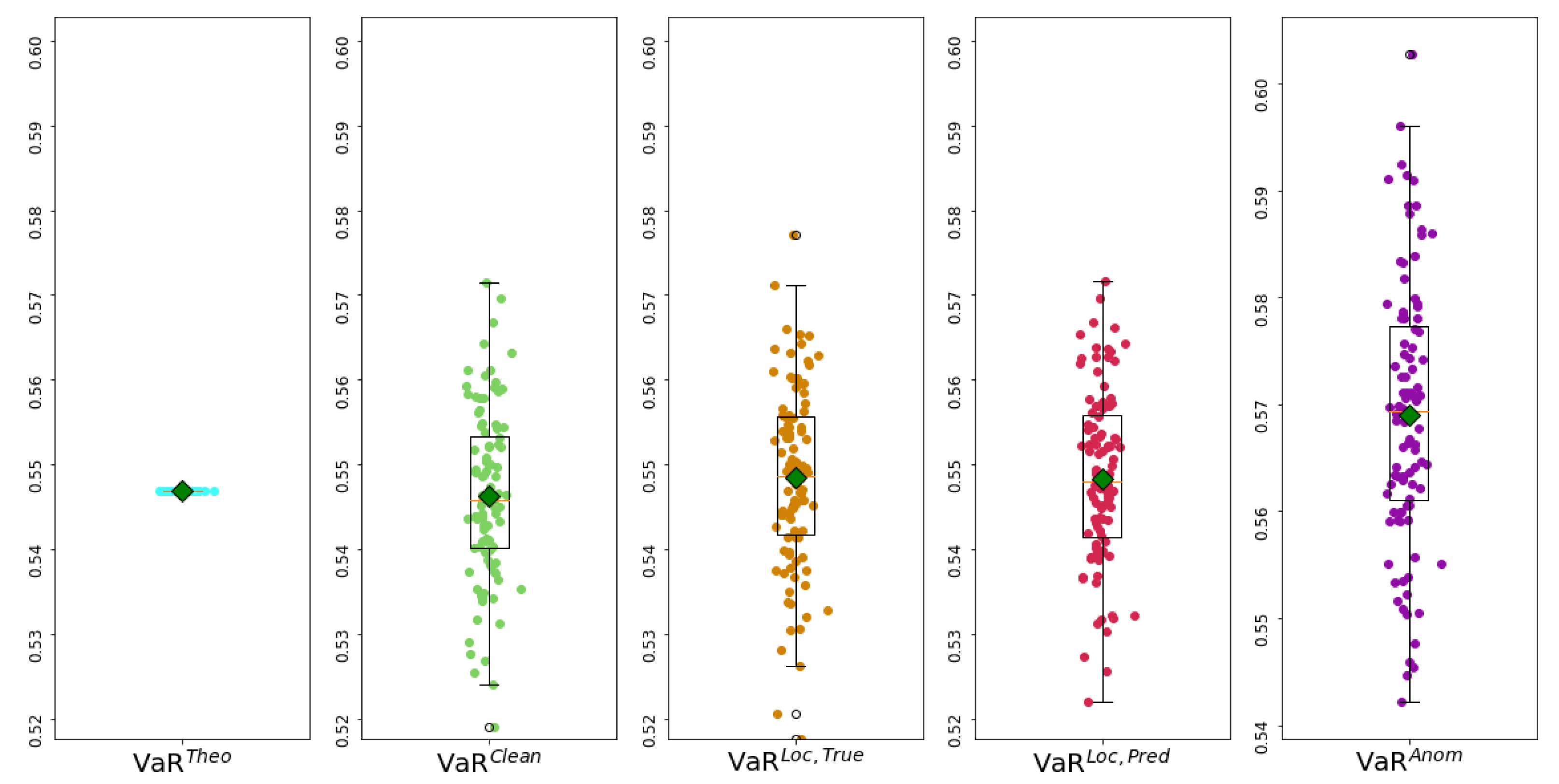
Figure 17.
Box plot representation of the parametric VaR estimations for P. The green squares represent the mean of the VaR estimations.
Figure 17.
Box plot representation of the parametric VaR estimations for P. The green squares represent the mean of the VaR estimations.
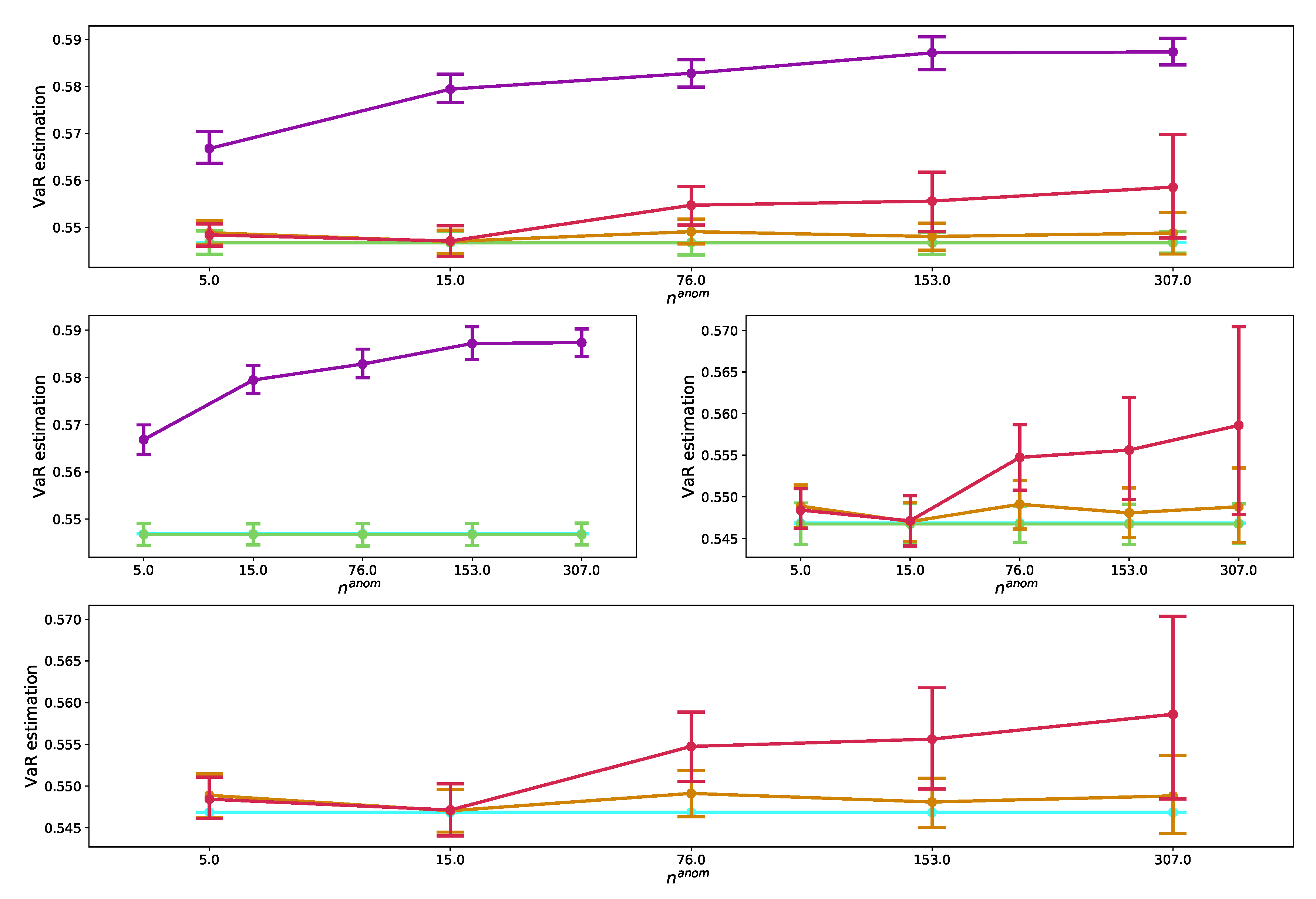
Figure 18.
VaR estimations based on parameter estimations from time series with and without anomalies (purple and light-blue curves), time series after localization and imputation of anomalies with the suggested approach (red curve), and time series imputed knowing the true localization of the anomalies (brown curve) with respect to .
Table 1.
AUC obtained with the naive and the NN approaches for the training set (left) and the test set (right).
Table 1.
AUC obtained with the naive and the NN approaches for the training set (left) and the test set (right).
| Approach | | | Approach | | |
|---|
| Naive | 0.1725 | 0.7898 | Naive | 0.1897 | 0.6354 |
| NN | 0.05153 | 0.1550 | NN | 0.1290 | 0.1367 |
Table 2.
Data set composition (top) before and (bottom) after data augmentation.
Table 2.
Data set composition (top) before and (bottom) after data augmentation.
| | Nb of Time Series | Nb of Observed Values per Time Series | Nb of Anomalies |
|---|
| Train set | 20 | 1000 | |
| Test set | 20 | 500 | |
| | Nb of Time Series | Nb of Observed Values per Time Series | Nb of Anomalies |
| Train set | 12,000 | 206 | 6000 |
| Test set | 2500 | 206 | 400 |
Table 3.
Performance evaluation of suggested model on synthetic data set for identification step.
Table 3.
Performance evaluation of suggested model on synthetic data set for identification step.
| Data Set | Accuracy | Precision | Recall | -Score |
|---|
| Train set | 90.97% | 97.36% | 84.21% | 90.31% |
| Test set | 88.58% | 61.26% | 85.27% | 71.30% |
Table 4.
Mean (standard deviation) of performance metrics of the suggested model over multiple runs for the identification step.
Table 4.
Mean (standard deviation) of performance metrics of the suggested model over multiple runs for the identification step.
| Data Set | Accuracy | Precision | Recall | -Score |
|---|
| Train set | 79.02% (2.4%) | 78.69% (2.7%) | 79.74% (4.6%) | 79.13% (2.7%) |
| Test set | 77.79% (3.9%) | 41.87% (5.2%) | 80.16% (6.4%) | 54.82% (5.2%) |
Table 5.
Performance evaluation of the suggested model and (the dummy approach) on synthetic data set for the localization step of all types of anomalies.
Table 5.
Performance evaluation of the suggested model and (the dummy approach) on synthetic data set for the localization step of all types of anomalies.
| Data Set | Accuracy | Precision | Recall | -Score |
|---|
| Train set | 89.65% (34.87%) | 89.81% (40.53%) | 89.65% (34.88%) | 89.68% ( 36.56%) |
| Test set | 94.39% (27.78%) | 94.49% (31.52%) | 94.39% (27.78%) | 94.38% (28.94%) |
Table 6.
Performance evaluation of the suggested model and the dummy approach on synthetic data set for the localization step of non-extrema anomalies.
Table 6.
Performance evaluation of the suggested model and the dummy approach on synthetic data set for the localization step of non-extrema anomalies.
| Data Set | Accuracy | Precision | Recall | -Score |
|---|
| Train set | 84.22% (0%) | 84.55% (0%) | 84.28% (0%) | 89.68% (0%) |
| Test set | 91.92% (0%) | 92.10% (0%) | 91.92% (0%) | 91.90% (0%) |
Table 7.
Mean (standard deviation) of performance metrics of suggested model over multiple runs for localization step of all types of anomalies.
Table 7.
Mean (standard deviation) of performance metrics of suggested model over multiple runs for localization step of all types of anomalies.
| Data Set | Accuracy | Precision | Recall | -Score |
|---|
| Train set | 89.58% (4.3%) | 89.58% (4.3%) | 89.96% (4.1%) | 89.67% (4.3%) |
| Test set | 89.49% (4.8%) | 89.49% (4.8%) | 90.00% (4.5%) | 89.58% (4.7%) |
Table 8.
Mean (standard deviation) of performance metrics of suggested model over multiple runs for localization step of non-extreme anomalies.
Table 8.
Mean (standard deviation) of performance metrics of suggested model over multiple runs for localization step of non-extreme anomalies.
| Data Set | Accuracy | Precision | Recall | -Score |
|---|
| Train set | 85.23% (6.0%) | 85.23% (6.0%) | 85.87% (5.7%) | 85.36% (6.0%) |
| Test set | 85.17% (7.1%) | 85.17% (7.1%) | 86.04% (6.8%) | 85.30% (7.1%) |
Table 9.
Performance evaluation of unsupervised (upper part) and supervised (lower part) models for contaminated time series identification step.
Table 9.
Performance evaluation of unsupervised (upper part) and supervised (lower part) models for contaminated time series identification step.
| | Train | Test |
|---|
| Model | Accuracy | -Score | Accuracy | -Score |
| IF | 42.31% | 42.31% | 69.64% | 7.022% |
| LOF | 59.95% | 59.95% | 90.00% | 62.41% |
| DBSCAN | 50.00% | 66.67% | 16.65% | 28.53% |
| sig-IF | 49.48% | 49.23% | 72.32% | 15.19% |
| KNN | 94.68% | 94.39% | 64.82% | 26.69% |
| SVM | 81.96% | 82.33% | 44.39% | 27.44% |
| PCA NN | 90.97% | 90.31% | 88.58% | 71.30% |
Table 10.
Execution time in seconds for identification of contaminated time series step.
Table 10.
Execution time in seconds for identification of contaminated time series step.
| Algorithm | IF | LOF | DBSCAN | KNN | SVM | sig-IF | PCA NN |
|---|
| Exec. Time | 0.6915 | 0.2015 | 0.1275 | 1.725 | 4.572 | 2.776 | 0.003523 |
Table 11.
Performance evaluation of unsupervised (upper part) and supervised (lower part) models for anomaly localization step. Results for DBSCAN, sig-IF, and SVM are not provided due to high computational costs.
Table 11.
Performance evaluation of unsupervised (upper part) and supervised (lower part) models for anomaly localization step. Results for DBSCAN, sig-IF, and SVM are not provided due to high computational costs.
| Model | Accuracy | -Score | Accuracy | -Score |
|---|
| IF | 89.79% | 2.296% | 70.94% | 1.611% |
| LOF | 99.51% | 0% | 2.066% | 0.9816% |
| DBSCAN | N/A | NA | NA | NA |
| sig-IF | N/A | N/A | N/A | N/A |
| KNN | 99.99% | 99.99% | 95.56% | 2.794% |
| SVM | NA | NA | NA | NA |
| PCA NN | 89.65% | 89.68% | 94.39% | 94.38% |
Table 12.
Execution time in seconds for the anomaly localization step. Results for DBSCAN, sig-IF, and SVM are not provided due to high computational costs.
Table 12.
Execution time in seconds for the anomaly localization step. Results for DBSCAN, sig-IF, and SVM are not provided due to high computational costs.
| Algorithm | IF | LOF | DBSCAN | KNN | SVM | sig-IF | PCA NN |
|---|
| Exec. Time | 14.50 | 2.287 | N/A | 14.19 | N/A | N/A | 0.002004 |
Table 13.
Mean and standard deviation errors on covariance matrix after imputation of anomalies with baseline methods.
Table 13.
Mean and standard deviation errors on covariance matrix after imputation of anomalies with baseline methods.
| Method | Ano | PCA | LI | BF | Clean |
|---|
| Mean | 0.004208 | 0.001575 | 0.001554 | 0.001554 | 0.001552 |
| Standard deviation | 0.000272 | 0.000165 | 0.000170 | 0.000172 | 0.000173 |
Table 14.
Performance evaluation after shocking the calibrated cutoff values for the training set (upper) and the test set (below).
Table 14.
Performance evaluation after shocking the calibrated cutoff values for the training set (upper) and the test set (below).
| Accuracy | Precision | Recall | |
| 0.9097 | 0.9736 | 0.8421 | 0.9031 |
| 0.9097 | 0.9736 | 0.8421 | 0.9031 |
| 0.9097 | 0.9738 | 0.8419 | 0.9031 |
| 0.9098 | 0.9737 | 0.8424 | 0.9033 |
| 0.9092 | 0.9747 | 0.8403 | 0.9025 |
| 0.9098 | 0.9720 | 0.8439 | 0.9035 |
| 0.9042 | 0.9860 | 0.8201 | 0.8954 |
| 0.9103 | 0.9563 | 0.8599 | 0.9056 |
| 0 | 0.9097 | 0.9736 | 0.8421 | 0.9031 |
| 1 | 0.7771 | 0.9994 | 0.5546 | 0.7133 |
| −1 | 0.5183 | 0.5093 | 0.9998 | 0.6749 |
| 2 | 0.6284 | 1.0000 | 0.2567 | 0.4086 |
| −2 | 0.5001 | 0.5000 | 1.0000 | 0.6667 |
| Accuracy | Precision | Recall | |
| 0.8858 | 0.6126 | 0.8527 | 0.7130 |
| 0.8858 | 0.6126 | 0.8527 | 0.7130 |
| 0.8858 | 0.6126 | 0.8527 | 0.7130 |
| 0.8850 | 0.6105 | 0.8527 | 0.7116 |
| 0.8877 | 0.6179 | 0.8527 | 0.7166 |
| 0.8838 | 0.6074 | 0.8527 | 0.7095 |
| 0.8984 | 0.6502 | 0.8432 | 0.7342 |
| 0.8672 | 0.5653 | 0.8741 | 0.6866 |
| 0 | 0.8858 | 0.6126 | 0.8527 | 0.7130 |
| 1 | 0.9391 | 0.9435 | 0.6746 | 0.7867 |
| −1 | 0.2660 | 0.1848 | 1.0000 | 0.3120 |
| 2 | 0.8949 | 0.9814 | 0.3753 | 0.5430 |
| −2 | 0.1700 | 0.1670 | 1.0000 | 0.2862 |
Table 15.
Detection ratios of the correctly identified contaminated time series in the test set, with the time series grouped according to their anomalies’ shock amplitudes.
Table 15.
Detection ratios of the correctly identified contaminated time series in the test set, with the time series grouped according to their anomalies’ shock amplitudes.
| Amplitude Range () | Detection Ratio |
|---|
| [0.309, 1.46] | 0.77 |
| [1.46, 2.34] | 0.91 |
| [2.34, 2.92] | 0.96 |
| [2.92, 3.78] | 0.98 |
Table 16.
Detection ratios of the correctly localized anomalies on the test set, with the anomalies grouped according to their shock amplitudes.
Table 16.
Detection ratios of the correctly localized anomalies on the test set, with the anomalies grouped according to their shock amplitudes.
| Amplitude Range () | Detection Ratio |
|---|
| [0.309, 1.31] | 0.86 |
| [1.31, 2.29] | 1.00 |
| [2.29, 2.88] | 1.00 |
| [2.88, 3.78] | 1.00 |
Table 17.
Notations of VaR estimations based on the time series from which the VaR parameters were estimated.
Table 17.
Notations of VaR estimations based on the time series from which the VaR parameters were estimated.
| VaR Estimation Name | Estimated on |
|---|
| Time series without anomalies |
| Times series with anomalies |
| Time series after anomaly imputation knowing their true localization |
| Time series after anomaly imputation based on predicted localization |
Table 18.
Summary of VaR estimations for P.
Table 18.
Summary of VaR estimations for P.
| VaR | | | | | |
|---|
| Mean | 0.546851 | 0.546300 | 0.548392 | 0.548270 | 0.569015 |
| Standard Deviation | 0.0 | 0.010105 | 0.010739 | 0.010832 | 0.012268 |
Table 19.
Mean absolute and relative errors in VaR estimations for P.
Table 19.
Mean absolute and relative errors in VaR estimations for P.
| VaR | | | | |
|---|
| Absolute Error | 0.007995 | 0.008596 | 0.008622 | 0.02235 |
| Relative Error | 0.014620 | 0.015720 | 0.015767 | 0.04087 |
Table 20.
Mean relative error of parametric VaR estimations with respect to for parameters estimated from clean time series, time series with anomalies, imputed time series following predicted location (), and true anomaly localization ().
Table 20.
Mean relative error of parametric VaR estimations with respect to for parameters estimated from clean time series, time series with anomalies, imputed time series following predicted location (), and true anomaly localization ().
| | | | |
|---|
| 5 | 0.012194 | 0.013796 | 0.013341 | 0.037392 |
| 15 | 0.012194 | 0.012623 | 0.016676 | 0.059604 |
| 76 | 0.012194 | 0.014831 | 0.024807 | 0.065791 |
| 153 | 0.012194 | 0.014644 | 0.034361 | 0.073750 |
| 307 | 0.012194 | 0.020537 | 0.052244 | 0.074091 |
Table 21.
Standard deviation of relative errors of parametric VaR estimations with respect to for parameters estimated from clean time series, time series with anomalies, imputed time series following predicted location (), and true anomaly localization ().
Table 21.
Standard deviation of relative errors of parametric VaR estimations with respect to for parameters estimated from clean time series, time series with anomalies, imputed time series following predicted location (), and true anomaly localization ().
| | | | |
|---|
| 5 | 0.010356 | 0.011511 | 0.009678 | 0.020674 |
| 15 | 0.010356 | 0.010514 | 0.012723 | 0.020172 |
| 76 | 0.010356 | 0.011842 | 0.018696 | 0.019930 |
| 153 | 0.010356 | 0.013683 | 0.026117 | 0.024243 |
| 307 | 0.010356 | 0.022526 | 0.057903 | 0.019207 |
Table 22.
Performance of the PCA NN identification step (upper part) and localization step (lower part) on the real data set.
Table 22.
Performance of the PCA NN identification step (upper part) and localization step (lower part) on the real data set.
| Data Set | Accuracy | Precision | Recall | -Score |
| Train set | 92.88% | 99.17% | 86.49% | 92.40% |
| Test set | 88.15% | 72.45% | 46.10% | 56.35% |
| Data Set | Accuracy | Precision | Recall | -Score |
| Train set | 99.48% | 99.49% | 99.48% | 99.48% |
| Test set | 96.05% | 96.21% | 96.05% | 95.92% |
Table 23.
Performance evaluation of unsupervised (upper part) and supervised (lower part) models in the contaminated time series identification step.
Table 23.
Performance evaluation of unsupervised (upper part) and supervised (lower part) models in the contaminated time series identification step.
| Model | Accuracy | Precision | Recall | -Score |
|---|
| IF | 73.17% | 18.12% | 17.53% | 17.82% |
| LOF | 82.33% | 44.57% | 26.62% | 33.33% |
| DBSCAN | 22.74% | 15.71% | 83.77% | 26.46% |
| sig-IF | 73.34% | 18.15% | 17.47% | 17.80% |
| KNN | 70.26% | 23.48% | 35.06% | 28.13% |
| SVM | 50.11% | 24.46% | 96.10% | 39.00% |
| PCA NN | 88.15% | 72.45% | 46.10% | 56.35% |
Table 24.
Performance evaluation of unsupervised (upper part) and supervised (lower part) models in the contaminated time series localization step. Results for DBSCAN, sig-IF, and SVM are not provided due to high computational costs.
Table 24.
Performance evaluation of unsupervised (upper part) and supervised (lower part) models in the contaminated time series localization step. Results for DBSCAN, sig-IF, and SVM are not provided due to high computational costs.
| Model | Accuracy | Precision | Recall | -Score |
|---|
| IF | 78.50% | 2.173% | 98.35% | 4.252% |
| LOF | 87.04% | 0.3713% | 9.616% | 0.7151% |
| DBSCAN | N/A | N/A | N/A | N/A |
| sig-IF | N/A | N/A | N/A | N/A |
| KNN | 99.85% | 78.38% | 95.59% | 86.13% |
| SVM | N/A | N/A | N/A | N/A |
| PCA NN | 96.05% | 96.21% | 96.05% | 95.92% |


