Dynamics and Stability on a Family of Optimal Fourth-Order Iterative Methods

Abstract

In this manuscript, we propose a parametric family of iterative methods of fourth-order convergence, and the stability of the class is studied through the use of tools of complex dynamics. We obtain the fixed and critical points of the rational operator associated with the family. A stability analysis of the fixed points allows us to find sets of values of the parameter for which the behavior of the corresponding method is stable or unstable; therefore, we can select the regions of the parameter in which the methods behave more efficiently when they are applied for solving nonlinear equations or the regions in which the schemes have chaotic behavior.

1. Introduction

One of the most important legacies in numerical analysis in the 20th century is the resolution of nonlinear equations by using high-order iterative methods, since we often encounter nonlinear mathematical models for which there are no analytical methods that allow us to find a solution of the nonlinear equation $f\left(x\right)=0$. This topic has attracted researchers from different areas, such as Traub in [1], who initiated the analysis of these methods.

Recently, Petković et al. (in [2]) and Amat et al. (in [3]) collected and updated the state of the art of multipoint methods. The advantage of this type of method is that it does not use higher-order derivatives, and it is of great practical importance because it overcomes the theoretical limitations of one-point methods. The latter are not good alternatives for increasing the order of convergence and the computational efficiency rate.

When the order of an iterative method increases, so does the number of functional evaluations per step. Ostrowski’s efficiency index (see [4]) gives a measure of the balance between these quantities, according to the formula $p^{\frac{1}{d}}$, where p is the order of convergence of the method and d is the number of functional evaluations per iteration. According to the Kung–Traub conjecture [5], the order of convergence of any multipoint method without memory cannot exceed the limit $2^{n-1}$, which is called the optimal order. Therefore, the optimal order of a method with three functional evaluations per step is 4. King’s family of methods [6], of which Ostrowski’s method [4] is a particular case, as is Jarratt’s method [7] and some of the families of multistep methods studied extensively in Traub’s book [8], are optimal fourth-order methods, since they perform only three functional evaluations per step. In recent years, as the extensive literature shows, there has been a renewed interest in the search for multistep methods in order to achieve optimal order convergence and, thus, better efficiency.

The rest of this paper is organized as follows. Section 2 is devoted to the presentation of a family of iterative methods that will be subjected to a dynamical analysis in Section 3. The stability of fixed points is studied, and the stable and unstable elements of the family are selected by means of the generation of the parameter plane. Some numerical tests are performed in Section 4, showing the performance of selected stable and unstable methods in comparison with other known ones. Finally, some conclusions are shown in Section 5.

2. The Proposed Family

In this section, we present particular cases of optimal fourth-order iterative methods for solving the nonlinear equation $f\left(x\right)=0$, $f:D\subseteq \mathbb{R}\to \mathbb{R}$, which was proposed in [9] by using the weight function procedure, the iterative expression of which is:

$$\left\{\begin{array}{c}{y}_n=x_n-{\displaystyle \frac{f\left(x_n\right)}{f^{\prime }\left(x_n\right)}}\hfill \\ x_{n+1}=x_n-{\displaystyle \frac{f\left(x_n\right)}{f^{\prime }\left(x_n\right)}}H\left(u\left(x_n\right)\right),\hfill \end{array}\right.$$

(1)

where $u\left(x_n\right)={\displaystyle \frac{f\left(y_n\right)}{f\left(x_n\right)}}$ and $H\left(u\right)$ is a real-valued weight function that achieves an optimal fourth-order convergence by using three functional evaluations. The following result indicates the necessary conditions that the weight function in question (1) has to fulfil so that the order of convergence reached is four [9].

Theorem 1.

Let f be a sufficiently differentiable function $f:D\subseteq \mathbb{R}\to \mathbb{R}$ with a single-zero ξ on the open interval D. Let $H\left(u\right)$ be a real-valued differentiable function. If an initial approximation $x_0$ is sufficiently close to the required root ξ of equation $f\left(x\right)=0$, then the order of convergence of the scheme (1) is four when $H\left(u\right)$ satisfies the following conditions:

$$H\left(0\right)=1,H^{\prime }\left(0\right)=1,H^{″}\left(0\right)=4and\left|H^{‴}\left(0\right)\right|<+\infty .$$

(2)

In this case, the error equation is

$$e_{n+1}=\left[\left(5-\frac{1}{6}{H}^{‴}\left(0\right)\right)c_2^3-c_2{c}_3\right]e_n^4+\mathcal{O}\left(e_n^5\right),$$

(3)

where

$$e_n=x_n-\xi and{c}_k=\frac{1}{k!}\frac{f^{\left(k\right)}\left(\xi \right)}{f^{\prime }\left(\xi \right)},k=2,3,4,\dots$$

Special Cases

In this section, we present some particular classes of iterative schemes obtained from expression (1) for different weight functions $H\left(u\right)$ that satisfy the conditions of Theorem 1.

• Firstly, we consider the well-known Ostrowski method, which is a particular case given by the following weight function:

  $$\begin{array}{cc}\hfill & H\left(u\right)={\displaystyle \frac{1-u}{1-2u}}.\hfill \end{array}$$

  (4)
  This weight function guarantees the fourth-order convergence of Ostrowski’s scheme, whose iterative expression is:

  $$\begin{array}{cc}\hfill & \left\{\begin{array}{c}{y}_n=x_n-{\displaystyle \frac{f\left(x_n\right)}{f^{\prime }\left(x_n\right)}},\hfill \\ x_{n+1}=x_n-{\displaystyle \frac{f\left(x_n\right)}{f^{\prime }\left(x_n\right)}}\left[{\displaystyle \frac{f\left(x_n\right)-f\left(y_n\right)}{f\left(x_n\right)-2f\left(y_n\right)}}\right].\hfill \end{array}\right.\hfill \end{array}$$

  (5)
• The following weight function is now considered:

  $$H\left(u\right)={\displaystyle \frac{1+u^2-u^3}{1-u}},$$

  (6)

  which satisfies all of the conditions of Theorem 1. This scheme was proposed by Maheshwari in [10], and its iterative expression is:

  $$\begin{array}{cc}\hfill & \left\{\begin{array}{c}{y}_n=x_n-{\displaystyle \frac{f\left(x_n\right)}{f^{\prime }\left(x_n\right)}},\hfill \\ x_{n+1}=x_n-{\displaystyle \frac{f\left(x_n\right)}{f^{\prime }\left(x_n\right)}}\left[{\displaystyle \frac{f\left(x_n\right)}{f\left(x_n\right)-f\left(y_n\right)}}+{\left({\displaystyle \frac{f\left(y_n\right)}{f\left(x_n\right)}}\right)}^2\right].\hfill \end{array}\right.\hfill \end{array}$$

  (7)
• The following uniparametric family satisfies the conditions of Theorem 1:

  $$\begin{array}{cc}\hfill & H\left(u\right)={\displaystyle \frac{\alpha +u(1+\alpha +u+2\alpha u)}{\alpha +u}},\hfill \end{array}$$

  (8)

  where $\alpha$ is a real parameter, and it provides a new iterative class of iterative schemes:

  $$\begin{array}{cc}\hfill & \left\{\begin{array}{c}{y}_n=x_n-{\displaystyle \frac{f\left(x_n\right)}{f^{\prime }\left(x_n\right)}},\hfill \\ x_{n+1}=x_n-{\displaystyle \frac{f\left(x_n\right)}{f^{\prime }\left(x_n\right)}}\left[{\displaystyle \frac{\alpha f{\left(x_n\right)}^2+f\left(x_n\right)f\left(y_n\right)(1+\alpha )+(1+2\alpha )f{\left(y_n\right)}^2}{f\left(x_n\right)[f\left(y_n\right)+\alpha f\left(x_n\right)]}}\right].\hfill \end{array}\right.\hfill \end{array}$$

  (9)
• Finally, using the convergence conditions to define the Taylor polynomial associated with the generic function $H\left(u\right)$, we obtain the last weight function presented here, thus satisfying Theorem 1.

  $$\begin{array}{cc}\hfill & H\left(u\right)={\displaystyle \frac{H^{‴}\left(0\right)}{6}}{u}^3+2u^2+u+1.\hfill \end{array}$$

  (10)
  We know that $|H^{‴}\left(0\right)|<\infty$, so if we substitute $H^{‴}\left(0\right)$ with $\beta$, we have a parametric family of iterative schemes of fourth-order convergence:

  $$\begin{array}{cc}\hfill & \left\{\begin{array}{c}{y}_n=x_n-{\displaystyle \frac{f\left(x_n\right)}{f^{\prime }\left(x_n\right)}},\hfill \\ x_{n+1}=x_n-{\displaystyle \frac{f\left(x_n\right)}{f^{\prime }\left(x_n\right)}}\left[{\displaystyle \frac{\beta }{6}}{\left({\displaystyle \frac{f\left(y_n\right)}{f\left(x_n\right)}}\right)}^3+2{\left({\displaystyle \frac{f\left(y_n\right)}{f\left(x_n\right)}}\right)}^2+\left({\displaystyle \frac{f\left(y_n\right)}{f\left(x_n\right)}}\right)+1\right].\hfill \end{array}\right.\hfill \end{array}$$

  (11)

Now, we will study the stability of the family given by Equation (11).

3. The Scaling Theorem

If the conjugation classes and the scaling theorem are verified for the method under study, it is possible to generalize a dynamical study on the polynomial of the second degree on which this study is performed. In this case, by applying this to a generic polynomial, such as $p\left(z\right)=(z-a)(z-b)$, we can assume that the result obtained will be equivalent to the result that we will obtain with any quadratic polynomial, since there will always be an affine transformation that takes us from this generic polynomial to any quadratic polynomial (see, for example, [11]). We emphasize that this result is only fulfilled in methods that contain derivatives, which is the justification of this study.

Let $\widehat{\mathbb{C}}$ be the Riemann sphere. Let $R_f:\widehat{\mathbb{C}}\to \widehat{\mathbb{C}}$ be the fixed-point operator of iterative scheme (11) on a function f, that is,

$$R_f\left(z\right)=z-\left(\frac{\beta }{6}{u}^3+2u^2+u+1\right)\frac{f\left(z\right)}{f^{\prime }\left(z\right)},$$

(12)

where

$$u=\frac{f\left(y\right)}{f\left(z\right)}\mathrm{and}y=z-\frac{f\left(z\right)}{f^{\prime }\left(z\right)}.$$

In order to generalize the dynamical analysis of family (11), we prove the following result.

Theorem 2

(Scaling Theorem). Let $A\left(z\right)=\alpha z+\mu$, $\alpha \ne 0$ be an affine mapping. In addition, let $f\left(z\right)$ be a holomorphic function and $h\left(z\right)=\lambda (f\circ A)\left(z\right)$ with $\lambda \ne 0$; then, the fixed-point operator ${\overline{R}}_f$ is an affine conjugate to ${\overline{R}}_h$ by A, i.e.,

$$\left(A\circ \overline{R_h}\circ A^{-1}\right)\left(z\right)=\overline{R_f}\left(z\right).$$

Proof. 

We will prove the following identity:

$$\left(\overline{R_f}\circ A\right)\left(z\right)=\left(A\circ \overline{R_h}\right)\left(z\right),\mathrm{for}\mathrm{all}z\in \widehat{\mathbb{C}}.$$

$$\begin{array}{cc}\hfill R_f\left(z\right)& =z-\left(\frac{\beta }{6}{u}^3+2u^2+u+1\right)\frac{f\left(z\right)}{f^{\prime }\left(z\right)}\hfill \\ \hfill & =z-\left[\frac{\beta }{6}{\left(\frac{f\left(y\right)}{f\left(z\right)}\right)}^3+2{\left(\frac{f\left(y\right)}{f\left(z\right)}\right)}^2+\left(\frac{f\left(y\right)}{f\left(z\right)}\right)+1\right]\frac{f\left(z\right)}{f^{\prime }\left(z\right)}.\hfill \end{array}$$

(13)

By developing the left side,

$$\begin{array}{c}\hfill \left(\overline{R_f}\circ A\right)\left(z\right)=A\left(z\right)-\left[\frac{\beta }{6}{\left(\frac{f\left(A\right(y\left)\right)}{f\left(A\right(z\left)\right)}\right)}^3+2{\left(\frac{f\left(A\right(y\left)\right)}{f\left(A\right(z\left)\right)}\right)}^2+\left(\frac{f\left(A\right(y\left)\right)}{f\left(A\right(z\left)\right)}\right)+1\right]\frac{f\left(A\right(z\left)\right)}{f^{\prime }\left(A\left(z\right)\right)}.\end{array}$$

(14)

Furthermore, we know that the fixed-point operator related to function h, for $\alpha \ne 0$, is:

$$\begin{array}{cc}\hfill R_h\left(z\right)& =z-\left(\frac{\beta }{6}{u}^3+2u^2+u+1\right)\frac{h\left(z\right)}{h^{\prime }\left(z\right)}\hfill \\ \hfill & =z-\left[\frac{\beta }{6}{\left(\frac{\lambda f\left(A\right(y\left)\right)}{\lambda f\left(A\right(z\left)\right)}\right)}^3+2{\left(\frac{\lambda f\left(A\right(y\left)\right)}{\lambda f\left(A\right(z\left)\right)}\right)}^2+\left(\frac{\lambda f\left(A\right(y\left)\right)}{\lambda f\left(A\right(z\left)\right)}\right)+1\right]\frac{\lambda f\left(A\right(z\left)\right)}{\lambda \alpha f^{\prime }\left(A\left(z\right)\right)}\hfill \\ \hfill & =z-\frac{1}{\alpha }\left[\frac{\beta }{6}{\left(\frac{f\left(A\right(y\left)\right)}{f\left(A\right(z\left)\right)}\right)}^3+2{\left(\frac{f\left(A\right(y\left)\right)}{f\left(A\right(z\left)\right)}\right)}^2+\left(\frac{f\left(A\right(y\left)\right)}{f\left(A\right(z\left)\right)}\right)+1\right]\frac{f\left(A\right(z\left)\right)}{f^{\prime }\left(A\left(z\right)\right)}.\hfill \end{array}$$

Considering that $A({\xi }_1-{\xi }_2)=A\left({\xi }_1\right)-A\left({\xi }_2\right)+\mu ,\mathrm{for}\mathrm{all}{\xi }_1,{\xi }_2\in \mathbb{C}$,

$$\begin{array}{cc}\hfill \left(A\circ \overline{R_h}\right)\left(z\right)=& A\left(z-\frac{1}{\alpha }\left[\frac{\beta }{6}{\left(\frac{f\left(A\right(y\left)\right)}{f\left(A\right(z\left)\right)}\right)}^3+2{\left(\frac{f\left(A\right(y\left)\right)}{f\left(A\right(z\left)\right)}\right)}^2+\left(\frac{f\left(A\right(y\left)\right)}{f\left(A\right(z\left)\right)}\right)+1\right]\frac{f\left(A\right(z\left)\right)}{f^{\prime }\left(A\left(z\right)\right)}\right)\hfill \\ \hfill =& A\left(z\right)-A\left(\frac{1}{\alpha }\left[\frac{\beta }{6}{\left(\frac{f\left(A\right(y\left)\right)}{f\left(A\right(z\left)\right)}\right)}^3+2{\left(\frac{f\left(A\right(y\left)\right)}{f\left(A\right(z\left)\right)}\right)}^2+\left(\frac{f\left(A\right(y\left)\right)}{f\left(A\right(z\left)\right)}\right)+1\right]\frac{f\left(A\right(z\left)\right)}{f^{\prime }\left(A\left(z\right)\right)}\right)+\mu \hfill \\ \hfill =& A\left(z\right)-\left[\frac{\beta }{6}{\left(\frac{f\left(A\right(y\left)\right)}{f\left(A\right(z\left)\right)}\right)}^3+2{\left(\frac{f\left(A\right(y\left)\right)}{f\left(A\right(z\left)\right)}\right)}^2+\left(\frac{f\left(A\right(y\left)\right)}{f\left(A\right(z\left)\right)}\right)+1\right]\frac{f\left(A\right(z\left)\right)}{f^{\prime }\left(A\left(z\right)\right)}.\hfill \end{array}$$

(15)

From the results obtained in (14) and (15),

$$\left(\overline{R_f}\circ A\right)\left(z\right)=\left(A\circ \overline{R_h}\right)\left(z\right).$$

Therefore, the method in (11) satisfies the scaling theorem. □

Now, we analyze the dynamical behavior of this class in terms of parameter $\beta$ in order to determine the methods with good stability properties and avoid the members of the family whose behavior is unstable.

4. Dynamical Analysis

In this part, we use several tools of complex dynamics. Thus, we need the function f to be defined on the Riemann sphere $\widehat{\mathbb{C}}$.

In the following, we recall some concepts of complex dynamics. Let us suppose a fixed-point function on an arbitrary polynomial $p\left(z\right)=(z-a)(z-b)$; this gives a rational function, $\mathcal{R}$.

Indeed, if given a rational function $\mathcal{R}:\widehat{\mathbb{C}}\to \widehat{\mathbb{C}}$, where $\widehat{\mathbb{C}}$ represents the Riemann sphere, the orbit at a point $z_0$ can be defined as

$$\{z_0,\mathcal{R}\left(z_0\right),{\mathcal{R}}^2\left(z_0\right),{\mathcal{R}}^3\left(z_0\right),\dots ,{\mathcal{R}}^n\left(z_0\right),\dots \}.$$

It is necessary to study the phase plane of $\mathcal{R}$ by classifying the fixed points according to the asymptotic behavior related to their orbits. A $z_0\in \widehat{\mathbb{C}}$ is said to be a fixed point if $\mathcal{R}\left(z_0\right)=z_0$. A periodic point $z_0$, of period $p>1$, is a point where ${\mathcal{R}}^p\left(z_0\right)=z_0$ and ${\mathcal{R}}^k\left(z_0\right)\ne z_0$, where $k<p$. A preperiodic point is a point $z_0$ that is not periodic, but there exists a $k>0$ such that ${\mathcal{R}}^k\left(z_0\right)$ is periodic. A point $z_0$ is a critical point of the rational function $\mathcal{R}$ if ${\mathcal{R}}^{\prime }\left(z_0\right)=0$. If a critical point is different from any of those related to the roots of polynomial $p\left(z\right)$, it is called a free critical point. In a similar way, the fixed points that are different from the roots of $p\left(z\right)$ are called strange fixed points.

Moreover, a fixed point $z_0$ is called an attractor if $\left|{\mathcal{R}}^{\prime }\left(z_0\right)\right|<1$, a superattractor if $\left|{\mathcal{R}}^{\prime }\left(z_0\right)\right|=0$, repulsive if $\left|{\mathcal{R}}^{\prime }\left(z_0\right)\right|>1$, and parabolic if $\left|{\mathcal{R}}^{\prime }\left(z_0\right)\right|=1$. Fixed points other than those associated with the roots of the polynomial $p\left(z\right)$ are called strange fixed points. The basin of attraction of an attractor $\alpha$ is defined as:

$$\mathcal{A}\left(\alpha \right)=\left\{z_0\in \widehat{\mathbb{C}}:{\mathcal{R}}^n\left(z_0\right)\to \alpha ,n\to \infty \right\}.$$

For the rational function $\mathcal{R}$, the Fatou set of $\mathcal{R}$, which is denoted by $\mathcal{F}\left(\mathcal{R}\right)$, is the set of points $z\in \widehat{\mathbb{C}}$ whose orbits tend to one attractor (a fixed point or periodic orbit). Its complement in $\widehat{\mathbb{C}}$ is the Julia set, $\mathcal{J}\left(\mathcal{R}\right)$. That is, the basin of attraction from every fixed or periodic point belongs to the Fatou set, while the boundaries of these basins of attraction are in the Julia set (for more explanation, see [12,13,14]).

The following result justifies the interest in the parameter planes that we will introduce later. The connected component of the basin of attraction, which contains the point or periodic orbit of attraction, is called the immediate basin of attraction.

Theorem 3

(Fatou–Julia). Let $\mathcal{R}$ be a rational function. An immediate basin of attraction of any attractor has at least one critical point.

To any rational operator that satisfies the scaling theorem, we can apply a Möbius transformation, which is stated as follows. If $p\left(z\right)=(z-a)(z-b)$, then ${\mathcal{R}}_p$ depends on parameters a and b. To eliminate this dependency, we apply a Möbius transformation h as follows:

$$O_p\left(z\right)=\left(h\circ {\mathcal{R}}_p\circ h^{-1}\right)\left(z\right),$$

where

$$h\left(z\right)=\frac{z-a}{z-b},$$

which satisfies

• $h(\infty )=1$,
• $h\left(a\right)=0$
• $h\left(b\right)=\infty$.

Operators $O_p$ and ${\mathcal{R}}_p$ have the same qualitative properties of stability.

With Theorem 2, we may find all of the stable behaviors of a rational function $\mathcal{R}$ by analyzing its performance on the set of critical points, as we see below.

Using polynomial $p\left(z\right)=(z-a)(z-b)$, the iterative scheme (11) on this polynomial provides the following rational operator:

$$M_p(z,\beta ,a,b)=z+\frac{(z-a)(z-b)\left(1+\frac{(z-a)(z-b)\left(6{(2z-a-b)}^{2}q\left(z\right)+{(z-a)}^2{(z-b)}^2\beta \right)}{6{(2z-a-b)}^6}\right)}{2z-a-b},$$

(16)

where $q\left(z\right)=a^2+4ab+b^2-6(a+b)z+6z^2$. By applying the Möbius transformation on $M_p(z,\beta ,a,b)$, we obtain the rational operator to work, which is an operator free of parameters a and b.

$$h\left(u\right)=\frac{u-a}{u-b},$$

and its inverse function is

$$h^{-1}\left(u\right)=\frac{ub-a}{u-1}.$$

To get the fixed-point operator,

$${\mathcal{R}}_p(z,\beta )=\left(h\circ M_p\circ h^{-1}\right)\left(z\right)=z^4\frac{\left(-6{(z+1)}^2(5+z(z+4))+\beta \right)}{-6{(z+1)}^2(1+z(5z+4))+z^4\beta }.$$

(17)

So, $M_p$ becomes a conjugate using the Möbius transformation for ${\mathcal{R}}_p(z,\beta )$ in order to simplify the dynamical analysis. Note that the rational operator ${\mathcal{R}}_p(z,\beta )$ is not reliant upon the roots of $p\left(z\right)$, a, and b.

4.1. Stability of the Fixed Points

In this section, we analyze the stability of fixed points. We give some important results on the stability of strange fixed points, and we analyze the behavior of the rational operator on free critical points. The strange fixed points are $z=1$, and the roots of the polynomial are

$$q(z,\beta )=6z^6+42z^5+126z^4+(180+\beta )z^3+126z^2+42z+6,$$

(18)

which is denoted by $s_j\left(\beta \right)$, $j=1,2,\dots ,6$.

The stability of the strange fixed points is analyzed in the following result.

Theorem 4.

The fixed points $z=0$ and $z=\infty$, which are associated with the roots a and b, are superattractors regardless of the value of β. $z=1$ is a strange fixed point when $\beta \ne 240$, and its stability is determined as follows:

(a) 

If $|\beta -240|>768$, then the fixed point $z=1$ is an attractor,

(b) 

If $|\beta -240|<768$, then the fixed point $z=1$ is repulsive,

(c) 

If $|\beta -240|=768$, then the fixed point $z=1$ is neutral.

Proof. 

By evaluating the rational operator ${\mathcal{R}}_p(z,\beta )$, as well as its derivative at $z=0$, we conclude that $z=0$ is a superattractor fixed point. For the punto $z=\infty$, we derive the inverse of the operator ${\mathcal{R}}_p(z,\beta )$, i.e., ${\left(\frac{1}{{\mathcal{R}}_p\left(\frac{1}{z}\right)}\right)}^{\prime }$, and we evaluate it in $z=0$. We can affirm that $z=\infty$ is a superattractor fixed point.

Now, we evaluate ${\mathcal{R}}_p^{\prime }(z,\beta )$ on the fixed point $z=1$ in order to determine its stability.

(a)

${\mathcal{R}}_p^{\prime }(1,\beta )=\left|\frac{768}{\beta -240}\right|<1$, which implies that $768<|\beta -240|$, and therefore $\left|{\mathcal{R}}_p^{\prime }(1,\beta )\right|<1$ if and only if $|\beta -240|>768$ and $\beta \ne 240.$

(b)

${\mathcal{R}}_p^{\prime }(1,\beta )=\left|\frac{768}{\beta -240}\right|>1$, which implies that $768<|\beta -240|$, and, therefore, $\left|{\mathcal{R}}_p^{\prime }(1,\beta )\right|>1$ if and only if $|\beta -240|<768$ and $\beta \ne 240$.

(c)

Finally, ${\mathcal{R}}_p^{\prime }(1,\beta )=\left|\frac{768}{\beta -240}\right|=1$, which implies that $768=|\beta -240|$, and, therefore, $\left|{\mathcal{R}}_p^{\prime }(1,\beta )\right|=1$ if and only if $|\beta -240|=768$ and $\beta \ne 240$.

This completes the proof. □

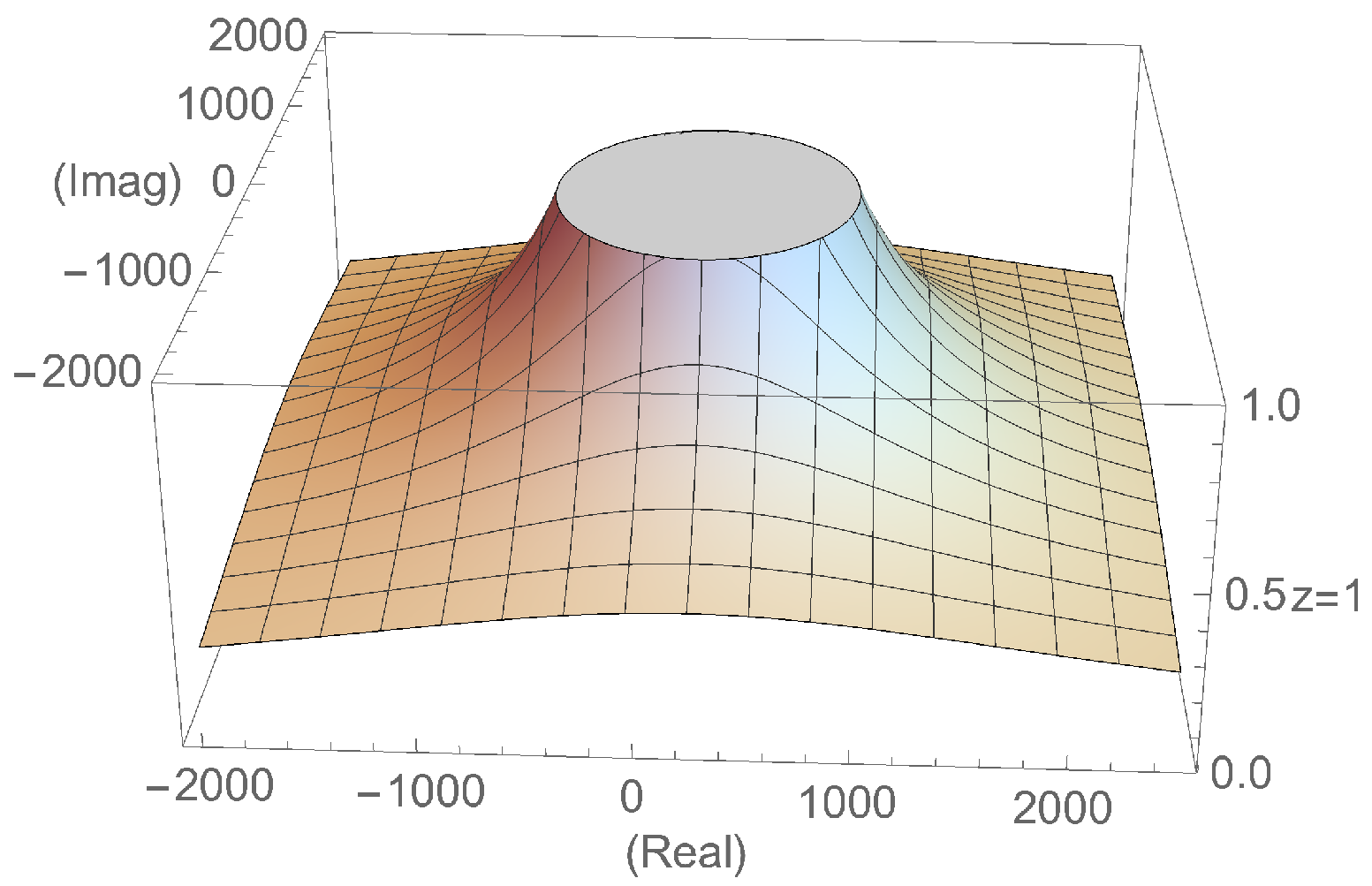
In Figure 1, the stability of the strange fixed point $z=1$ is presented.

Theorem 4 shows that we have two fixed points that are superattractors, $z=0$ and $z=\infty$, and the strange fixed point $z=1$, for which we find different regions where this behaves as an attractor, repulsor, and parabolic for $\beta \ne 240$. However, when we solve the equation ${\mathcal{R}}_p(z,\beta )=z$, six other solutions appear; these are strange fixed points that are solutions of the polynomial $q(z,\beta )$ (18), which is denoted by $s_j\left(\beta \right)$, $j=1,2,\dots ,6$. In the following result, we analyze the stability of these strange fixed points.

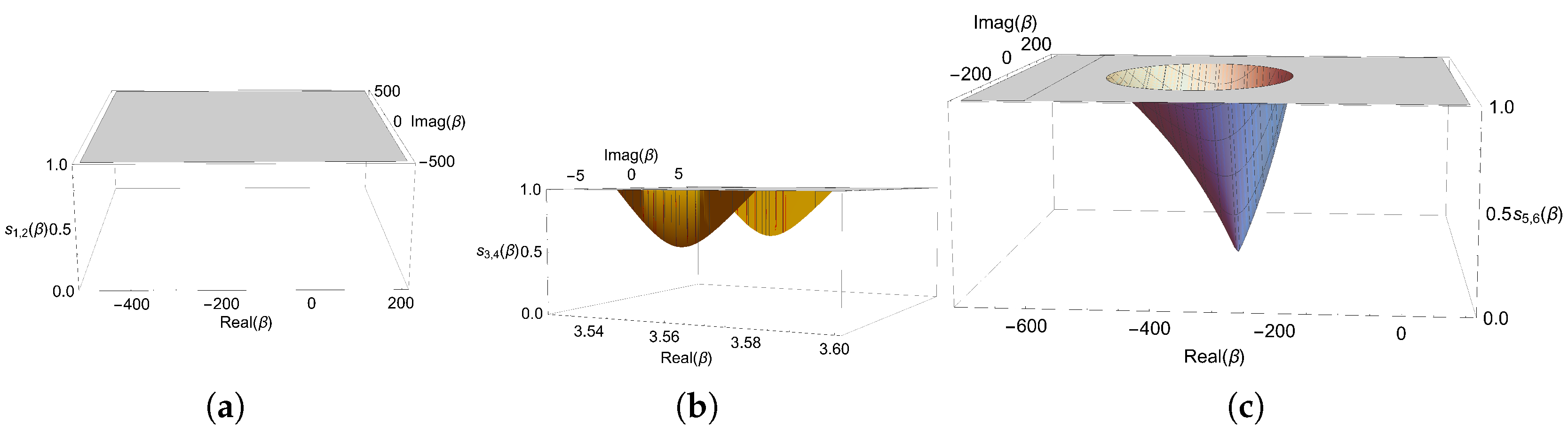
Theorem 5.

The strange fixed points of the rational operator ${\mathcal{R}}_p(z,\beta )$, $s_j\left(\beta \right)$, $j=1,2$, are all repulsors in a complex plane.

On the other hand, the strange fixed points $s_j\left(\beta \right),j=3,4$ are:

1. 

attractors in the open interval $\frac{32}{9}<\beta <3.55728$. In particular, they are superattractors for $\beta \approx 3.55728\mp 4.9603i$.

2. 

parabolics for $\beta =\frac{4}{9}(8\mp 5i\sqrt{5})$.

3. 

repulsors in the rest of the complex plane.

Finally, the strange fixed points $s_j\left(\beta \right),j=5,6$ are:

1. 

attractors in $-524.182<\beta <-289.865$ and $-289.865<\beta <-189.865)$. In particular, they are superattractors for $\beta \approx -289.865$.

2. 

parabolic at all points on the boundary of the circumference of the cone—in particular, for the complex numbers $\beta =\frac{4}{9}(8\mp 5i\sqrt{5})$.

3. 

repulsors in the rest of the complex plane.

Theorem 5 cannot be analytically proven, since the substitution of these strange fixed points into the stability function results in roots of higher-order polynomials. Still, the stability regions in the complex plane of the strange fixed points $s_1\left(\beta \right)$ and $s_2\left(\beta \right)$ can be visualized in Figure 2a, the stability regions of the fixed points $s_3\left(\beta \right)$ and $s_4\left(\beta \right)$ can be visualized in the complex plane in Figure 2b, and the stability regions of the fixed points $s_5\left(\beta \right)$ and $s_6\left(\beta \right)$ can be visualized in the complex plane in Figure 2c. Note that in the foreground, no stability region is visualized, which justifies the behavior of such strange fixed points; they are repulsors in the whole complex plane, and the strange fixed points $s_3\left(\beta \right)$ and $s_4\left(\beta \right)$ are attractors in the small region described in Theorem 5, while the strange fixed points $s_5\left(\beta \right)$ and $s_6\left(\beta \right)$, are parabolic in the boundary of the circumference of the cone and are attracting inside the cone, being superattracting at the vertex of the cone. They are repulsive in the rest of the complex plane.

4.2. Critical Points

The critical points are obtained by solving equation ${\mathcal{R}}_p{(z,\beta )}^{\prime }=0$. We obtain the points $z=0$, $z=\infty$, which correspond to the roots of polynomial $p\left(x\right)$, and the free critical points described in the following results.

Theorem 6.

The free critical points of operator ${\mathcal{R}}_p(z,\beta )$ are:

1. 

$c{r}_j\left(\beta \right)=\frac{120+3\beta \mp \sqrt{7\left(240\beta -{\beta }^2\right)}}{4(\beta -30)},j=1,2.$

2. 

$z=-1.$

Let us also remark that the critical points satisfy $c{r}_1\left(\beta \right)={\displaystyle \frac{1}{c{r}_2\left(\beta \right)}}$. So, they are not independent, and they have the same parameter plane.

There are also values of parameter $\beta$ for which the critical points coincide:

(a)

The critical points $c{r}_1\left(\beta \right)=c{r}_2\left(\beta \right)=c{r}_3\left(\beta \right)$ match for $\beta =0$.

(b)

The points $c{r}_1\left(\beta \right)=c{r}_2\left(\beta \right)$ match if $\beta =240$.

The free critical point $z=-1$ is a pre-image of the strange fixed point $z=1$ because $\mathcal{R}(-1,\beta )=1$; therefore, there is no need to obtain its related parameter plane because the information that would be obtained is contained in the stability function of $z=1$.

5. Parameter and Dynamical Planes

In this section, our goal is to determine the regions of the parameter plane for which we can obtain the most stable members of the family, since the values of $\beta$ in those regions will provide us with the best methods in terms of numerical stability.

5.1. Parameter Planes

As $c{r}_1\left(\beta \right)$ and $c{r}_2\left(\beta \right)$ are conjugates, there exists just one free independent critical point, the related parameter plane of which can be seen in Figure 3. This is focused in a black region that mostly corresponds to regions shown in the stability planes of the strange fixed points $s_3\left(\beta \right)$ and $s_4\left(\beta \right)$ and the bases of the cones defining the stability functions of the strange fixed points $s_5\left(\beta \right)$ and $s_6\left(\beta \right)$ (see Figure 2b,c). Let us assume that there are free independent critical points acting in the capacity of the starting point of the iterative schemes of the family associated with each complex value of $\beta$; such points are shown in red on the complex plane if the method converges on any of the roots (zero and infinity) and in black in other cases. Following this procedure, we obtain the parameter plane presented in Figure 3 by using the processes shown in [10]. For this representation, we used a mesh of $1500\times 1500$ points, a maximum of 500 iterations, and a tolerance of ${10}^{-3}$ in the stopping criterion. We also show a close-up of this parameter plane in Figure 3b, focusing on the larger red area; there, the family members are, in general, very stable. These will be the best values to use for iterative methods in terms of their stability (see [15]).

We emphasize how important the parameter planes are, since they allow us to precisely identify the values of the $\beta$ parameter for which the family of iterative methods have stable behavior or the members have chaotic behavior. In these, we can observe two black- and red-colored regions; the red-colored region allows us to obtain dynamic planes whose behavior is stable, and the black-colored regions imply methods that mostly correspond to values of the parameter in which there are strange fixed points that are attractors or have periodic attractor orbits; this is guaranteed by the (Fatou–Julia), Theorem 3.

5.2. Dynamical Planes

The dynamical planes appearing in Figure 4 and Figure 5 were obtained using a mesh of $2000\times 2000$ points of the complex plane, as well as a maximum of 1000 iterations. These show the basins of attraction that correspond to different values that we selected from the parameter plane—both from the red-colored zone, where we had more stable members of the family, and the black-colored zones of the parameter plane, where we had unstable members of the family. In both cases, different stable behaviors, unstable behaviors, and periodic basins of attraction, among others, are shown.

In each of the dynamical planes, the circles represent the fixed points of $\mathcal{R}(z,\beta )$ (with the independence of their stability), the squares represent the critical points, and the starred point represents the superattracting fixed points.

Unstable and Stable Dynamic Planes

For the values $\beta =0$, $\beta =1$, $\beta =10$, and $\beta =100$ (Figure 5a–d, respectively), we observe stable behavior corresponding to the red-colored regions in the parameter plane. The orange regions in the dynamical planes come from the superattracting fixed point $z=0$, and the blue area comes from the fixed point $z=\infty$. Finally, Figure 4a–d correspond to regions of the parameter plane where we obtain families whose behavior is unstable. Moreover, for $\beta =350$, we obtain a dynamical plane with two periodic orbits at points $z=0.254854-0.96698i$ and $z=0.897069+0.44189i$. It is worth noting that the dynamical plane corresponding to $z=-200-650i$ has three basins of attraction, which are shown in green, orange, and blue colors; for $z=-300$, there are four basins of attraction, which are shown in green, orange, blue, and red; for $z=-700$, there are three basins of attraction, unlike the stable dynamical planes, which only have two.

6. Numerical Results

We use the functions proposed in

Table 1. Test functions.

$\mathit{f}\left(\mathit{x}\right)$	$\mathit{\xi }$
$f_1\left(x\right)=e^{-x}+cosx$	$1.7461395304080124176507030889537802$
$f_2\left(x\right)=x^4+sin\left(\frac{\pi }{x^2}\right)-5$	$1.4142135623730950488016887242096980$
$f_3\left(x\right)=e^x-1.5-{tan}^{-1}x$	$0.7676532662012788981900298911398052$
$f_4\left(x\right)=10x{e}^{-x^2}-1$	$1.6796306104284499406749203388379704$

to perform some numerical tests in order to analyze the results obtained with different known methods in comparison with the one proposed in the iterative family (11).

We call the methods used for the numerical tests M1, M2, and M3. M3 is the method that we worked with in this manuscript, and M1 and M2 are two known fourth-order methods that we use to compare the numerical results; these are the scheme of C. Chun and the BCMT family, which can be found in [16,17].

$$\begin{array}{cc}& M1=\left\{\begin{array}{c}{y}_n=x_n-\frac{f\left(x_n\right)}{f^{\prime }\left(x_n\right)}\hfill \\ x_{n+1}=y_n-\frac{f\left(x_n\right)+2f\left(y_n\right)}{f\left(x_n\right)}\frac{f\left(y_n\right)}{f^{\prime }\left(x_n\right)},\hfill \end{array}\right.\hfill \end{array}$$

where $n=0,1,2\dots .$

$$\begin{array}{cc}\hfill & M2=\left\{\begin{array}{c}{y}_n=x_n-\frac{f\left(x_n\right)}{f^{\prime }\left(x_n\right)}\hfill \\ x_{n+1}=x_n-\frac{f\left(x_n\right)}{f^{\prime }\left(x_n\right)}\left[\frac{\alpha +2}{3{\alpha }^2}{\left(\frac{f\left(x_n\right)}{f\left(x_n\right)+\alpha f\left(y_n\right)}\right)}^3-\frac{2(1+\alpha )}{{\alpha }^2}\left(\frac{f\left(x_n\right)}{f\left(x_n\right)+\alpha f\left(y_n\right)}\right)+\frac{3{\alpha }^2+5\alpha +4}{3{\alpha }^2}\right].\hfill \end{array}\right.\hfill \end{array}$$

where $\alpha =1\mathrm{and}n=0,1,2,\dots$.

$$\begin{array}{cc}& M3=\left\{\begin{array}{c}{y}_n=x_n-{\displaystyle \frac{f\left(x_n\right)}{f^{\prime }\left(x_n\right)}},\hfill \\ x_{n+1}=x_n-{\displaystyle \frac{f\left(x_n\right)}{f^{\prime }\left(x_n\right)}}\left[{\displaystyle \frac{\beta }{6}}{\left({\displaystyle \frac{f\left(y_n\right)}{f\left(x_n\right)}}\right)}^3+2{\left({\displaystyle \frac{f\left(y_n\right)}{f\left(x_n\right)}}\right)}^2+\left({\displaystyle \frac{f\left(y_n\right)}{f\left(x_n\right)}}\right)+1\right].\hfill \end{array}\right.\hfill \end{array}$$

where $\beta =10\mathrm{and}n=0,1,2,\dots$.

The following expression can be used to estimate the theoretical order of convergence:

$$p\approx COC=\frac{ln\left|\left(x_{n+1}-\xi \right)/\left(x_n-\xi \right)\right|}{ln\left|\left(x_n-\xi \right)/\left(x_{n-1}-\xi \right)\right|},$$

as presented by S. Weerakoon and T.G.I. Fernando in [18]. However, the principal inconvenience of this $\mathrm{COC}$ is that it requires knowledge of the precise root $\xi$. In order to solve such a problem, in [19], Cordero and Torregrosa overhauled the definition of $\mathrm{COC}$ so that it would not need the root to be exactly known at all, as shown in the following:

$$p\approx ACOC=\frac{ln\left|x_{n+1}-x_n\right|/\left|x_n-x_{n-1}\right|}{ln\left|x_n-x_{n-1}\right|/\left|x_{n-1}-x_{n-2}\right|}.$$

Calculations were performed by using the Matlab programming software with variable-precision arithmetic, with 200 digits of mantissa and $ϵ={10}^{-8}$ as the error tolerance. For the computer programs, the following stopping criteria were used:

(i)

$\left|x_{n+1}-x_n\right|<ϵ$ or

(ii)

$\left|f\left(x_{n+1}\right)\right|<ϵ$.

Table 2. Benchmark comparison of fourth-order methods in relation to the convergence order and computational time on the function $f\left(x\right)$.

$\mathit{f}\left(\mathit{x}\right)$	Iterations			Computational Time in (s)			$\mathbf{ACOC}$
	M1	M2	M3	M1	M2	M3	M1	M2	M3
$f_1\left(x\right),2$	3	3	3	0.050211	0.044647	0.053968	4.1497	3.4747	4.1213
$f_2\left(x\right),2$	5	4	4	0.185660	0.103332	0.096203	3.9928	3.9584	4.0173
$f_3\left(x\right),1$	3	3	3	0.054889	0.058569	0.061012	3.7652	3.6640	3.8134
$f_4\left(x\right),1.9$	4	5	4	0.074889	0.123747	0.098324	3.9630	3.9885	3.9945

displays the best outcomes for each experiment. We can see how the following method is highly efficient compared to schemes such as Chun’s and the BCMT, which we used for comparison.

7. Conclusions

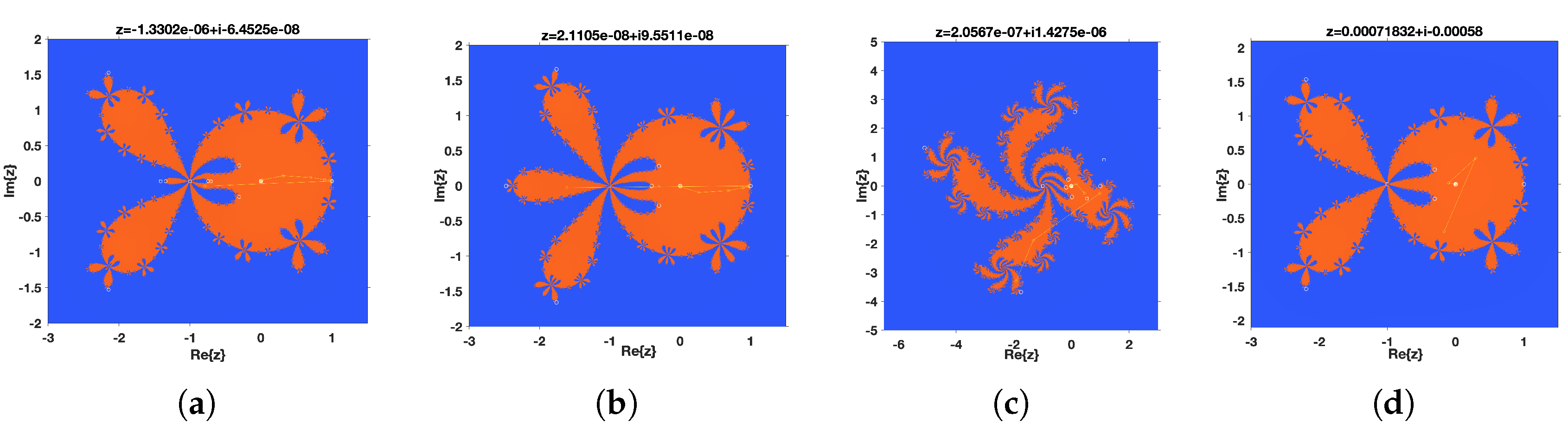
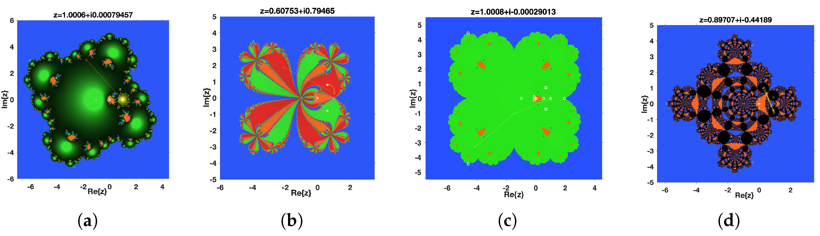
In our manuscript, we found a large, optimal, and general kind of fourth-order scheme that is free of second derivatives. The dynamical analysis that was performed on the proposed class of methods allowed us to choose family members that were particularly stable, discarding the ones with unstable performance, where strange fixed points and some periodical orbits were present. Lastly, we refer to Table 2 to show that the suggested family is equal to or more competitive than the classical method, the recognized and efficient methods of Ostrowski and Maheshwari, and other recognized and efficient methods found in the literature. The dynamic study shows us that there are values of the parameter $\beta$ for which we can obtain highly efficient iterative families of methods; some of the values that we can use are $\beta =0$, $\beta =1$, $\beta =10$, and $\beta =100$.

This behavior is justified in the dynamic planes given in Figure 5a–d, since there is global convergence to the roots of a second-degree polynomial.

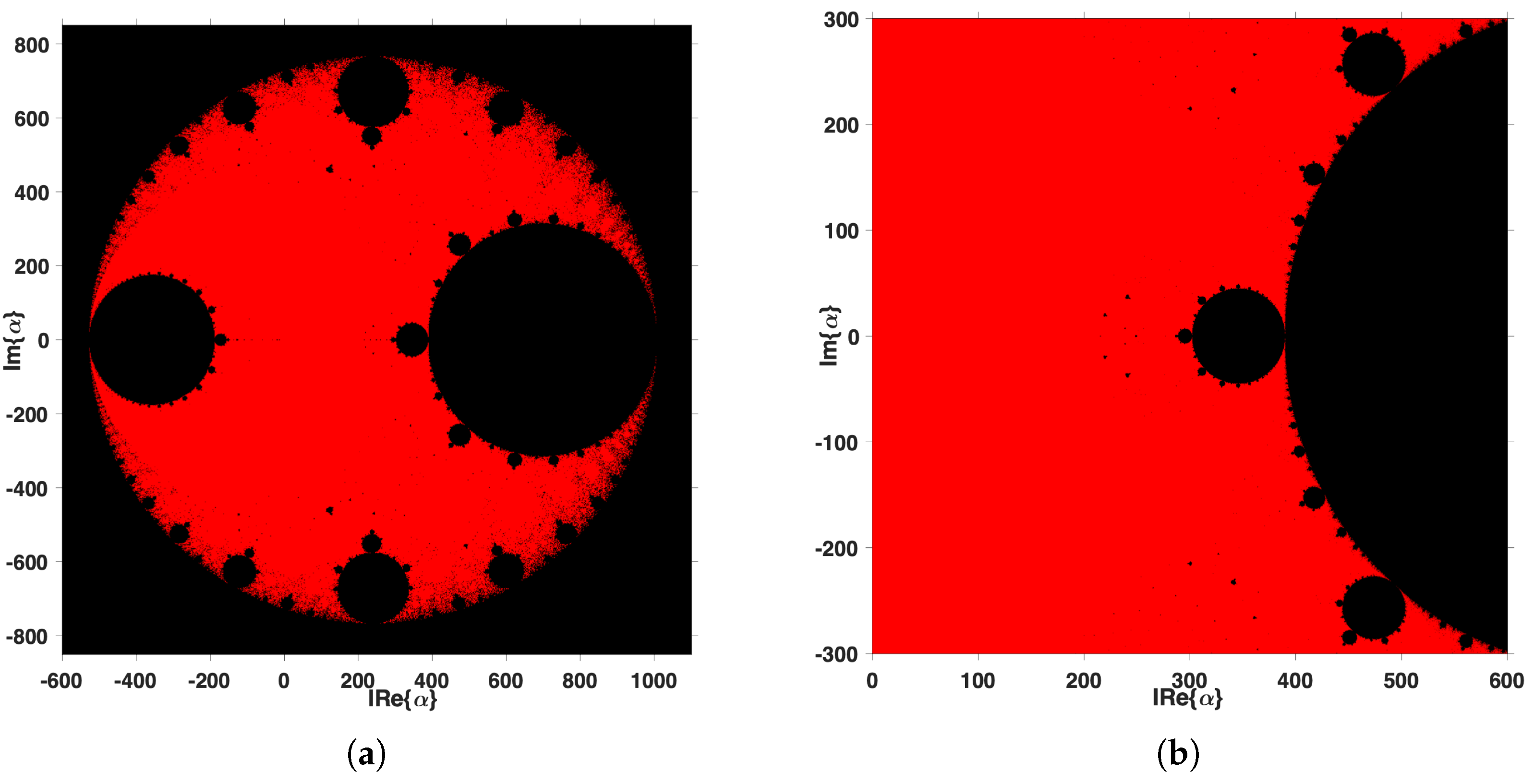
In addition, if we use parameter values corresponding to regions of instability, one of the consequences of using these schemes is that these do not converge to the root, and if they do converge, they would do so with a large number of iterations, that is, these members are unreliable. This fact can be confirmed in Figure 4a–d.

The results shown in Table 2 and

Table 3. Benchmark comparison of fourth-order methods in relation to the absolute error $\left|x_{n+1}-x_n\right|$ and $\left|f\left(x_{n+1}\right)\right|$.

$\mathit{f}\left(\mathit{x}\right)$	$\left|{\mathit{x}}_{\mathit{n}+1}-{\mathit{x}}_{\mathit{n}}\right|$			$\left|\mathit{f}\left({\mathit{x}}_{\mathit{n}+1}\right)\right|$
	M1	M2	M3	M1	M2	M3
$f_1\left(x\right)$	$7.3\times {10}^{-16}$	$2.59\times {10}^{-16}$	$1.67\times {10}^{-16}$	$1.16\times {10}^{-62}$	$2.87\times {10}^{-64}$	$2.58\times {10}^{-65}$
$f_2\left(x\right)$	$1.16\times {10}^{-27}$	$1.35\times {10}^{-13}$	$2.31\times {10}^{-19}$	$2.19\times {10}^{-207}$	$2.17\times {10}^{-50}$	$3.84\times {10}^{-74}$
$f_3\left(x\right)$	$5.69\times {10}^{-10}$	$9.24\times {10}^{-9}$	$1.33\times {10}^{-10}$	$5.64\times {10}^{-27}$	$8.89\times {10}^{-32}$	$1.11\times {10}^{-39}$
$f_4\left(x\right)$	$3.7\times {10}^{-19}$	$1.3\times {10}^{-25}$	$2.18\times {10}^{-28}$	$2.22\times {10}^{-73}$	$7.57\times {10}^{-99}$	$1.79\times {10}^{-110}$

are satisfactory from the point of view of numerical calculations. It can be observed that the number of iterations, computational time, and theoretical convergence order reached by our family, in comparison with the known methods of Chun and the BCMT, are satisfactory, as we expected, since we took one of the values of the $beta$ parameter for which it was theoretically shown that we would have efficient iterative methods. In addition, another piece of evidence that shows the degree of accuracy with which our method converges to the root is the computation of the absolute errors $\left|x_{n+1}-x_n\right|$ and $\left|f\left(x_{n+1}\right)\right|$, which are shown in Table 3.

References

1. Traub, I.F. Iterative Methods for the Solution of Equations; Prentice-Hall: Hoboken, NJ, USA, 1964. [Google Scholar]
2. Petković, M.S.; Neta, B.; Petković, L.D.; Džunić, J. Multipoint Methods for Solving Nonlinear Equations; Academic Press: Amsterdam, The Netherlands, 2013. [Google Scholar]
3. Amat, S.; Busquier, S. Advances in Iterative Methods for Nonlinear Equations; SEMA SIMAI Springer Series; Springer: Cham, Switzerland, 2016; Volume 10. [Google Scholar]
4. Ostrowski, A.M. Solutions of Equations and System of Equations; Academic Press: New York, NY, USA, 1960. [Google Scholar]
5. Kung, H.T.; Traub, J.F. Optimal order of one-point and multi-point iteration. ACM 1974, 21, 643–651. [Google Scholar]
6. King, R. A family of fourth order methods for nonlinear equations. SIAM J. Numer. Anal. 1973, 10, 876–879. [Google Scholar] [CrossRef]
7. Jarratt, P. Some fourth order multipoint methods for solving equations. Math. Comput. 1966, 20, 434–437. [Google Scholar] [CrossRef]
8. Traub, J.F. Iterative Methods for the Solution of Equations; Chelsea Publishing Company: New York, NY, USA, 1982. [Google Scholar]
9. Chicharro, F.I.; Cordero, A.; Garrido, N.; Torregrosa, J.R. Wide stability in a new family of optimal fourth-order iterative methods. Comput. Math. Methods 2019, 1, e1023. [Google Scholar] [CrossRef] [Green Version]
10. Maheshwari, A.K. A fourth order iterative method for solving nonlinear equation. Appl. Math. Comput. 2009, 211, 383–391. [Google Scholar] [CrossRef]
11. Wang, X.; Chen, X. The Dynamical Analysis of a Biparametric Family of Six-Order Ostrowski-Type Method under the Möbius Conjugacy Map. Fractal Fract. 2022, 6, 174. [Google Scholar] [CrossRef]
12. Fatou, P. Sur les substitutions rationnelles. Comp. Rend. Heb. S. Acad. Sci. 1917, 164, 806–808, 1917, 165, 992–995. [Google Scholar]
13. Julia, G. Mémoire sur l’iteration des fonctions rationnelles. Mat. Pur. Appl. 1918, 8, 47–245. [Google Scholar]
14. Blanchard, P. Complex analytic dynamics on the riemann sphere. Bull. Am. Math. Soc. 1984, 11, 85–141. [Google Scholar] [CrossRef] [Green Version]
15. Chicharro, F.I.; Cordero, A.; Torregrosa, J.R. Drawing Dynamical and Parameters Planes of Iterative Families and Methods. Sci. World J. 2013, 2013, 780153. [Google Scholar] [CrossRef] [PubMed] [Green Version]
16. Behl, R.; Cordero, A.; Motsa, S.S.; Torregrosa, J.R. An optimal fourth-order family of methods for multiple roots and its dynamics. Numer. Algor. 2016, 71, 775–796. [Google Scholar] [CrossRef]
17. Chun, C. Construction of Newton-like iterative methods for solving nonlinear equations. Numer. Math. 2006, 104, 297–315. [Google Scholar] [CrossRef]
18. Weerakoon, S.; Fernando, T.G.I. A variant of Newton’s method with accelerated third-order convergence. Appl. Math. Letters. 2000, 13, 87–93. [Google Scholar] [CrossRef]
19. Cordero, A.; Torregrosa, J.R. Variants of Newton’s method using fifth-order quadrature formulas. Appl. Math. Comput. 2007, 190, 686–698. [Google Scholar]
Figure 1. Strange fixed point stability region where z = 1 .
Algorithms 15 00387 g001
Figure 2. Strange fixed points s j ( β ) , j = 1 , , 6 . (a) s 1 ( β ) and s 2 ( β ) . (b) s 3 ( β ) and s 4 ( β ) . (c) s 5 ( β ) and s 6 ( β ) .
Algorithms 15 00387 g002
Figure 3. Parameter planes ( β ) for free critical points. (a) Parameter plane with z = c r 1 ( β ) . (b) Zoomed-in view of the parameter plane.
Algorithms 15 00387 g003
Figure 4. Dynamical planes whose behavior is unstable. (a) β = 200 650 i . (b) β = 300 . (c) β = 700 . (d) β = 350 .
Algorithms 15 00387 g004
Figure 5. Dynamical planes whose behavior is stable. (a) β = 1 . (b) β = 10 . (c) β = 100 200 i . (d) β = 0 .
Algorithms 15 00387 g005