Artificial Neural Network-Based Surrogate Modeling for Energy-Efficient Operation of the Oilfield Gathering and Transportation System

Abstract

The oilfield gathering and transportation system (OGTS) accounts for a substantial share of total energy consumption, demonstrating considerable potential for energy-saving optimization. Previous research primarily focused on the independent optimization of gathering pipeline networks or processing stations, with little attention given to their integrated optimization. This study investigates the OGTS of a domestic oilfield block. It develops artificial neural network (ANN) surrogate models for both pipelines and processing station equipment to accurately capture system operating states. An optimization model linking the pipeline network and processing station is established, and a differential evolution algorithm is applied to enhance computational efficiency. The results indicate that optimal predictive performance was achieved when the first hidden layer of the backpropagation neural network (BPNN) contained 50 neurons with a rectified linear unit (ReLU) activation function, with the surrogate models achieving coefficient of determination (R²) values exceeding 0.85. Under a 30 min optimization cycle, total system energy consumption decreased by 2.28%, with computation completed in under 3 min, while daily average optimization led to a 1.55% reduction. These findings demonstrate that the proposed integrated optimization framework offers both a robust methodological foundation and practical engineering guidance for coordinated, low-carbon, and energy-efficient operation of oilfields.

1. Introduction

In recent years, growing global concern over greenhouse gas emissions has driven the implementation of numerous carbon-mitigation initiatives, including the Paris Agreement, the European Green Deal, and China’s commitments to carbon peaking and neutrality [1,2,3]. The oilfield gathering and transportation system (OGTS) is highly energy-intensive, and its rising energy use underscores the need for optimization technologies [4,5]. Developing production operation plans is a critical strategy for optimizing energy consumption [6]. Improving OGTS energy efficiency supports both sustainable oilfield development and China’s broader economic and environmental objectives.

The OGTS consists of the oil-gas gathering system and processing system, facilitating crude oil metering, separation, centralized processing, and transportation [7]. Featuring numerous nodes and equipment, its structural and operational complexity stems from diverse network topologies (e.g., branch, star, ring) [8,9,10] and dehydration methods (e.g., chemical, physical) [11,12,13]. Consequently, accurately modeling complex pipeline networks and diverse equipment presents a significant obstacle to optimal OGTS management [14].

Extensive research targets energy reduction in gathering pipeline networks by optimizing transport modes and operating parameters [15,16,17]. To minimize costs, Pan et al. proposed an integrated optimization framework for the design and operation of gathering pipeline networks, demonstrating carbon emission reductions of 42.8% and 66.8% in two case studies [7]. Expanding beyond operational schemes, Liu et al. introduced equipment-level decision variables, such as variable-frequency pump speeds, to optimize pipeline energy consumption [18]. Wei et al. developed a mixed-integer nonlinear programming framework for steady-state pipeline network optimization, aiming to reduce compressor unit energy use [19]. Despite these advances, most research overlooks the integrated optimization of pipelines and processing stations. Chen et al. modeled a four-level station layout based on the separation performance of processing stations [20]. However, the numerous production parameters [4] and the large scale of the OGTS complicate model construction and hinder real-time optimization due to computational limits [21,22]. Therefore, developing accurate yet efficient models is vital to enhancing the operational efficiency of oilfields.

Artificial neural networks (ANNs) offer efficient, cost-effective modeling for complex systems like the OGTS [23]. Ghafariasl et al. applied neural network-based surrogate models to a multi-generation system, achieving multi-objective optimization improvements of 1.9–12.7% [24]. Given the scale of the OGTS, steady-state real-time optimization requires robust algorithms capable of rapid solution generation [25]. Among various intelligent algorithms, the differential evolution (DE) algorithm is widely studied for its global search capability and rapid convergence [26,27]. Trevisan et al. applied the DE algorithm to an offshore oil and gas production network, effectively solving steady-state optimization problems [14]. This approach substantially improves computational efficiency in complex engineering optimization tasks [28,29].

Specifically, previous ANN-based surrogate models primarily target individual equipment or local parameters, often relying on physical models of other subsystems. Building on previous research, this study develops high-precision ANN prediction models for core equipment within the gathering pipeline network and the processing station. These models form the basis of an integrated optimization framework that minimizes operational energy consumption of both subsystems, yielding optimal operational schemes for the OGTS.

2. Methodology

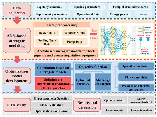
Figure 1 presents the research framework, which encompasses data collection, ANN-based surrogate modeling, optimization model development, a case study, and results and discussion. The ANN surrogate models were used to predict the operating parameters of the OGTS following adjustments to the optimization variables. This enables the calculation of total system energy consumption and the verification of constraint conditions. These results are then converted into fitness values for the algorithm, guiding the selection, crossover, and mutation operations of the DE algorithm until the search converges.

Figure 1. Research framework of the present study.

2.1. Design Concept of the OGTS Surrogate Model

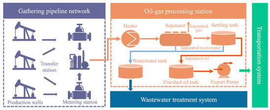
As shown in Figure 2, the OGTS primarily consists of a cluster of production wells, a gathering pipeline network, an oil-gas processing station, a wastewater treatment system, and a transportation system. The processing station is equipped with heaters, three-phase separators, settling tanks, and export pumps to support oil-gas separation and handling [30]. Well-produced fluids are transported to the processing station via the gathering pipeline network, where heating promotes oil-water separation. The separated wastewater is treated accordingly, while the qualified crude oil is transferred to downstream processes.

Figure 2. Process flow of the OGTS.

Given the complexity of physical modeling for oilfield equipment and its limited applicability at the system level [31,32], an ANN-based surrogate modeling approach was adopted [33]. ANN models were developed using real operational data collected from field facilities, with each equipment model constructed independently. These equipment-level models were then integrated according to the process flow to form a comprehensive OGTS surrogate model.

Because individual equipment models were developed independently, mass balance must be ensured during system integration [34]. Fluid flow rates were transferred sequentially from one equipment model to the next. Similarly, parameters at the interfaces between adjacent units, including temperature, flow rate, and water cut, were maintained consistently. Given specific initial conditions, the surrogate model directly predicted the following outputs:

• Terminal temperature and terminal pressure of the pipeline;
• Outlet temperature of the heater;
• Outlet temperature and outlet water cut of the separator;
• Outlet temperature and outlet water cut of the settling tank;
• Outlet pressure of the export pump.

2.2. Artificial Neural Network Surrogate Models

Before model training, data preparation and feature engineering were carried out. During data preprocessing, missing values were reconstructed using Lagrange interpolation, and outliers were removed to ensure a reliable dataset for model development. In feature engineering, input variables were normalized to the range 0–1 to eliminate the influence of differences in feature scales on model training. Candidate input variables were then evaluated using Pearson correlation coefficients, and features exhibiting high correlation with model outputs were selected as inputs. The input features and output variables for each surrogate model are summarized in Table 1. Notably, for each output variable, an independent single-output model was constructed for prediction.

Table 1. Input features and output variables of each surrogate model.

Model	Input Features	Output Variables
Pipeline	Flow rate, water cut, inlet temperature and pressure, pipeline length and diameter	Terminal temperature and terminal pressure
Heater	Flow rate, water cut, inlet temperature, flue gas temperature	Outlet temperature
Separator	Flow rate, water cut, inlet pressure, inlet temperature, oil layer level	Outlet temperature, outlet water cut
Settling tank	Flow rate, water cut, oil-water interface height, liquid level	Outlet temperature, outlet water cut
Export pump	Flow rate, frequency, motor effective voltage and effective current	Outlet pressure

Overall, ANNs possess strong nonlinear fitting capabilities, enabling them to capture complex relationships between input variables and output responses from historical data [35,36]. Consequently, they have been widely applied to modeling and prediction problems in engineering systems [37,38]. For surrogate model development in the OGTS, the selected data-driven model needed to satisfy three criteria: robust generalization performance, short training time, and a flexible network architecture with broad adaptability. Considering these requirements, a backpropagation neural network (BPNN) was employed in this study to establish equipment-level surrogate models.

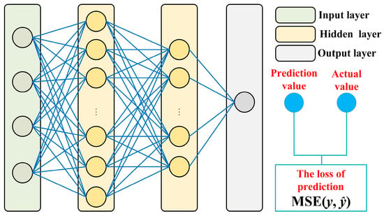
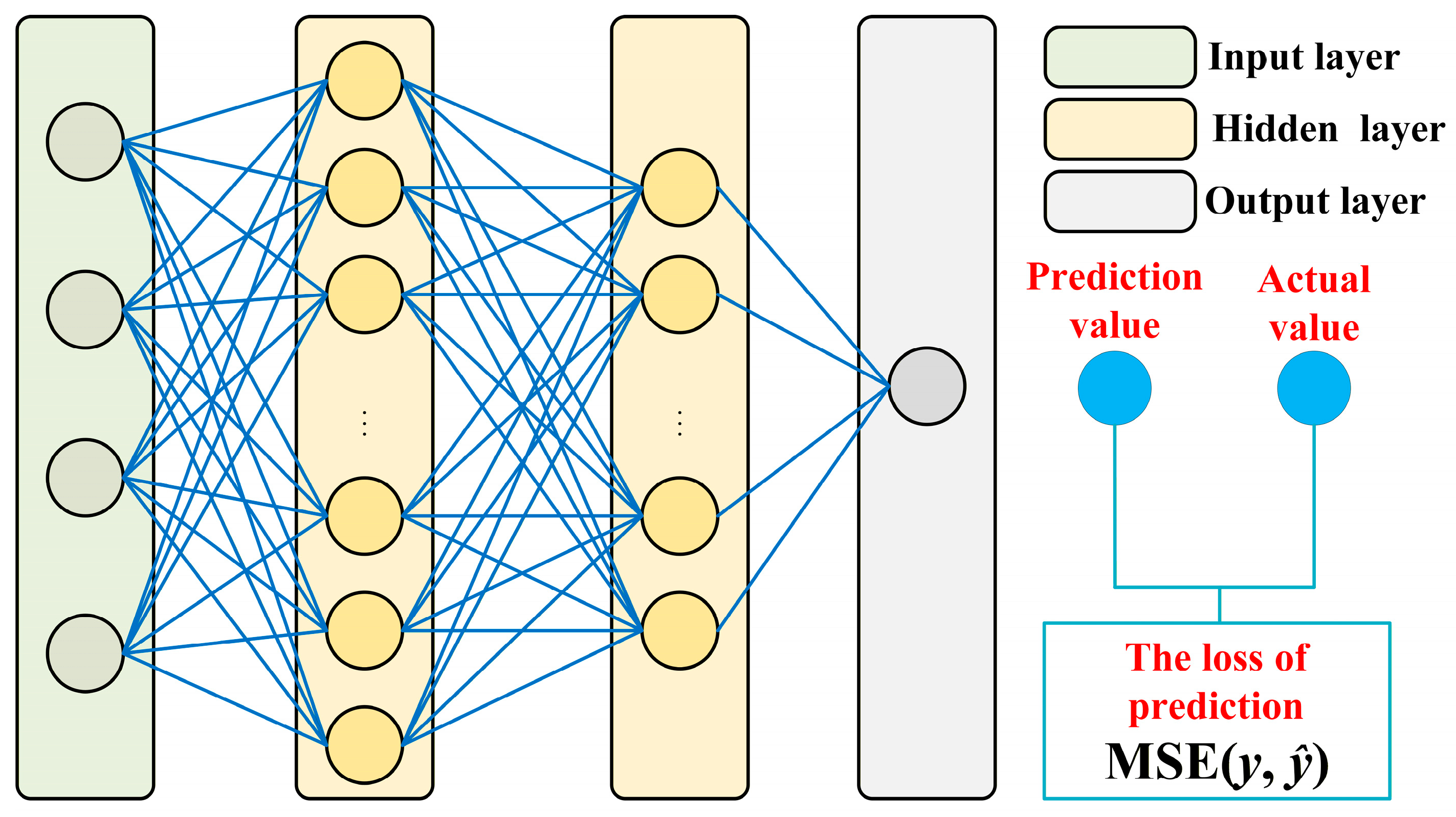
Furthermore, the BPNN is a fully connected, multilayer feedforward neural network trained via error backpropagation. It consists of an input layer, multiple hidden layers, and an output layer. Figure 3 illustrates the BPNN architecture employed in this study. The network comprises three types of layers: an input layer that receives feature vectors, two hidden layers for feature processing, and an output layer that generates prediction values. The first hidden layer contains 50 neurons with a ReLU activation function for preliminary feature extraction, while the second hidden layer consists of 25 neurons, also using the ReLU activation function, to further refine these feature representations. The output layer adopts a linear activation function to produce continuous prediction values. These predictions are compared against actual values to calculate prediction loss, quantified by mean squared error (MSE), which serves as the objective function for network training via error backpropagation. This hierarchical design enables gradual condensation of latent features while maintaining representational capacity. For a detailed analysis of neuron number selection and activation function configuration, please refer to Section 3.2.

Figure 3. Structure of the BPNN.

To improve optimization efficiency and ensure stable training, the Adam optimizer was employed to update network parameters, with a learning rate of 0.001 [27]. The batch size and maximum number of training epochs were set to 10 and 300, respectively. To mitigate the risk of overfitting, an early stopping mechanism was implemented. Training was halted automatically if the validation loss failed to improve over 10 consecutive epochs, ensuring the model retained its generalization capability. The dataset was partitioned into training, validation, and test sets, comprising 70%, 15%, and 15% of the data, respectively [39,40].

Prediction performance across all surrogate models was evaluated using root mean squared error (RMSE), normalized root mean squared error (NRMSE), coefficient of determination (R²), and mean absolute error (MAE) [41,42]. The corresponding definitions are provided in Equations (1)–(4).

$$\mathrm{RMSE}=\sqrt{{\displaystyle \frac{1}{n}}{\displaystyle {\sum }_{k=1}^n{\left(y_k-{\widehat{y}}_k\right)}^2}}$$

(1)

$$\mathrm{NRMSE}={\displaystyle \frac{\sqrt{\frac{1}{n}{\displaystyle {\sum }_{k=1}^n{\left(y_k-{\widehat{y}}_k\right)}^2}}}{y_{\max }-y_{\min }}}$$

(2)

$${\mathrm{R}}^2=1-{\displaystyle \frac{{{\displaystyle \sum }}_{k=1}^n{\left(y_k-{\widehat{y}}_k\right)}^2}{{{\displaystyle \sum }}_{k=1}^n{\left(y_k-\overline{y}\right)}^2}}$$

(3)

$$\mathrm{MAE}={\displaystyle \frac{1}{n}}{\displaystyle \sum }_{k=1}^n\left|y_k-{\widehat{y}}_k\right|$$

(4)

where y_k and ŷ_k represent the true and predicted values of the k-th sample, ӯ denotes the mean of the actual observations, y_max and y_min are the maximum and minimum values of the variable, and n is the number of test samples. It is worth noting here that NRMSE eliminates the influence of different physical units, allowing a unified evaluation of prediction accuracy for output variables across different equipment [43,44].

2.3. Operation Optimization Model

2.3.1. Objective Function

The energy consumption of the OGTS comprises both fuel consumption and electricity consumption. As noted in Equations (5) and (6), the total energy consumption rate of the OGTS (F^EC) is expressed as a function of fuel and electricity usage:

$$\min F^{\mathrm{EC}}=E^{\mathrm{FUEL}}+E^{\mathrm{ELE}}$$

(5)

$$\left\{\begin{array}{l}{E}^{\mathrm{FUEL}}={\displaystyle \sum _{i\in N}\frac{G_i{c}_i\left(T_{\mathrm{out},i}-T_{\mathrm{in},i}\right)}{{\eta }_{f,i}}}\\ E^{\mathrm{ELE}}={\displaystyle \sum _{j\in M}\frac{\left(P_{\mathrm{out},j}-P_{\mathrm{in},j}\right)V_j}{{\eta }_{p,j}}}\end{array}\right.$$

(6)

where F^EC denotes the total energy consumption rate (kW), E^FUEL and E^ELE denote the fuel and electricity power consumption, respectively (kW), N and M represent the numbers of fuel-consuming units and electricity-consuming units in the system, G_i is the mass flow rate of fluid passing through unit i (kg/s), c_i is the specific heat capacity of the fluid in unit i (kJ/(kg·°C)), T_out,i and T_in,i are the outlet and inlet temperatures of unit i, respectively, η_f,i is the thermal efficiency of unit i (%), P_out,j and P_in,j are the outlet and inlet pressures of unit j, respectively (kPa), V_j is the volumetric flow rate of fluid through unit j (m³/s), and η_p,j is the pump efficiency of unit j (%).

2.3.2. Constraints

(1)

Process constraints

Equation (7) defines the upper limit of the production rate for the production wells. Equations (8) and (9) ensure that the outlet water cut of crude oil and the oil content of wastewater from the separation unit meet production requirements.

$$Q_p^{\mathrm{liq}}\le Q_p^{\mathrm{liq},\max } \forall p\in PL$$

(7)

$$W{C}_d\le W{C}_d^{\max } \forall d\in DU$$

(8)

$$O{C}_d\le O{C}_d^{\max } \forall d\in DU$$

(9)

where $Q_p^{\mathrm{l}\mathrm{i}\mathrm{q}}$ and $Q_p^{\mathrm{l}\mathrm{i}\mathrm{q}\mathrm{,}\mathrm{m}\mathrm{a}\mathrm{x}}$ denote the liquid flow rate and maximum liquid flow rate of pipeline p, respectively, (m³/s), WC_d and ${WC}_d^{\mathrm{m}\mathrm{a}\mathrm{x}}$ represent the outlet crude oil water cut of separation unit d and its upper limit, respectively (%), PL denotes the set of pipelines, DU represents the set of dehydration units, and OC_d and ${OC}_d^{\mathrm{m}\mathrm{a}\mathrm{x}}$ denote the outlet oil content in produced water from separation unit d and its upper limit (%).

(2)

Flow constraints

(a)

Flow balance for the pipeline network

Equation (10) ensures that, within the gathering pipeline network, the total inflow to a node is equal to its total outflow. The first term denotes the cumulative flow rates entering the node from all connected pipelines. The second term represents the aggregate flow directed into the processing station. The third term accounts for the flow rates of separated crude oil and wastewater leaving the processing station. The fourth term represents the total flow rates leaving the node through all connected pipelines.

$${\displaystyle \sum _{i\in PN}{Q}_i^{\mathrm{pi}}}+{\displaystyle \sum _{j\in PS}{Q}_j}={\displaystyle \sum _{j\in PS}\left(Q_j^{\mathrm{w}}+Q_j^{\mathrm{o}}\right)}+{\displaystyle \sum _{i\in PN}{Q}_i^{\mathrm{po}}}$$

(10)

where $Q_i^{\mathrm{p}\mathrm{i}}$ denotes the flow rate entering the node from pipeline i (m³/s), Q_j represents the flow rate entering processing station j (m³/s), $Q_j^{\mathrm{w}}$ denotes the wastewater flow rate leaving the processing station j (m³/s), $Q_j^{\mathrm{o}}$ denotes the crude oil flow rate leaving the processing station j (m³/s), $Q_i^{\mathrm{p}\mathrm{o}}$ represents the flow rate leaving the node through pipeline i (m³/s), PN represents the set of pipeline nodes, and PS denotes the set of processing stations.

• (b)

  Flow balance of the processing station

Within the processing station, crude oil can either be stored in equipment such as separators and settling tanks or conveyed to the next stage of production using oil transfer pumps. The corresponding flow balance is formulated as follows:

$$Q_{\mathrm{in}}^{\mathrm{ps}}+{\displaystyle \sum _{i\in SEP}\left(Q_{\mathrm{in},i}^{\mathrm{sep}}-Q_{\mathrm{out},i}^{\mathrm{sep}}\right)+{\displaystyle \sum _{j\in TAN}\left(Q_{\mathrm{in},j}^{\tan }-Q_{\mathrm{out},j}^{\tan }\right)}}=Q_{\mathrm{out}}^{\mathrm{ps}}$$

(11)

where $Q_{\mathrm{i}\mathrm{n}}^{\mathrm{p}\mathrm{s}}$ and $Q_{\mathrm{o}\mathrm{u}\mathrm{t}}^{\mathrm{p}\mathrm{s}}$ denote the liquid flow rates entering and leaving the processing station, respectively (m³/s), $Q_{\mathrm{i}\mathrm{n},i}^{\mathrm{s}\mathrm{e}\mathrm{p}}$ and $Q_{\mathrm{o}\mathrm{u}\mathrm{t},i}^{\mathrm{s}\mathrm{e}\mathrm{p}}$ denote the inlet and outlet flow rates of separator i within the processing station (m³/s), $Q_{\mathrm{i}\mathrm{n},j}^{\mathrm{t}\mathrm{a}\mathrm{n}}$ and $Q_{\mathrm{o}\mathrm{u}\mathrm{t},j}^{\mathrm{t}\mathrm{a}\mathrm{n}}$ represent the inlet and outlet flow rates of tank j in the processing station (m³/s), SEP refers to the set of all separators, and TAN denotes the set of all settling tanks.

• (c)

  Storage volume constraints of settling tanks

The volume of a settling tank is determined solely by its inflow and outflow rates, subject to the following constraints:

$$V_{i,t}=V_{i,t-1}+\left(Q_{i,t}^{\mathrm{li}}-Q_{i,t}^{\mathrm{lo}}\right)\mathrm{\Delta }t \forall i\in TAN,t\in T$$

(12)

At any given time, the tank volume must remain within specified upper and lower limits:

$$V_i^{\min }\le V_{i,t}\le V_i^{\max } \forall i\in TAN,t\in T$$

(13)

where V_i,t and V_i,t−1 denote the liquid volume of tank i at time t and t − 1, respectively (m³), $Q_{i,t}^{\mathrm{l}\mathrm{i}}$ and $Q_{i,t}^{\mathrm{l}\mathrm{o}}$ denote the inflow and outflow rates of tank i at time t (m³/s), $V_i^{\mathrm{m}\mathrm{i}\mathrm{n}}$ and $V_i^{\mathrm{m}\mathrm{a}\mathrm{x}}$ correspond to the minimum and maximum storage capacities of tank i, respectively (m³), and T represents the set of time periods considered.

(3)

Operation constraints

The operating constraints for the inlet and outlet of the gathering pipeline network are defined as follows:

$$P_i^{\mathrm{pip},\min }\le P_i^{\mathrm{pip}}\le P_i^{\mathrm{pip},\max } \forall i\in PL$$

(14)

$$T_i^{\mathrm{pip},\min }\le T_i^{\mathrm{pip}}\le T_i^{\mathrm{pip},\max } \forall i\in PL$$

(15)

where $P_i^{\mathrm{p}\mathrm{i}\mathrm{p}}$ denotes the operating pressure of pipeline i (kPa), $P_i^{\mathrm{p}\mathrm{i}\mathrm{p},\mathrm{m}\mathrm{i}\mathrm{n}}$ and $P_i^{\mathrm{p}\mathrm{i}\mathrm{p},\mathrm{m}\mathrm{a}\mathrm{x}}$ represent its minimum and maximum allowable pressures, respectively (kPa), and $T_i^{\mathrm{p}\mathrm{i}\mathrm{p}}$ denotes the operating temperature of pipeline i (°C), with $T_i^{\mathrm{p}\mathrm{i}\mathrm{p},\mathrm{m}\mathrm{i}\mathrm{n}}$ and $T_i^{\mathrm{p}\mathrm{i}\mathrm{p},\mathrm{m}\mathrm{a}\mathrm{x}}$ defining its lower and upper temperature limits, respectively (°C).

The operational constraints for the inlet and outlet of processing station equipment are formulated as follows:

$$P_i^{\mathrm{equ},\min }\le P_i^{\mathrm{equ}}\le P_i^{\mathrm{equ},\max } \forall i\in EQU$$

(16)

$$T_i^{\mathrm{equ},\min }\le T_i^{\mathrm{equ}}\le T_i^{\mathrm{equ},\max } \forall i\in EQU$$

(17)

where $P_i^{\mathrm{e}\mathrm{q}\mathrm{u}}$ denotes the operating pressure of processing station equipment i (kPa), $P_i^{\mathrm{e}\mathrm{q}\mathrm{u},\mathrm{m}\mathrm{i}\mathrm{n}}$ and $P_i^{\mathrm{e}\mathrm{q}\mathrm{u},\mathrm{m}\mathrm{a}\mathrm{x}}$ represent the respective lower and upper pressure limits (kPa), $T_i^{\mathrm{e}\mathrm{q}\mathrm{u}}$ represents the operating temperature of equipment i (°C), $T_i^{\mathrm{e}\mathrm{q}\mathrm{u},\mathrm{m}\mathrm{i}\mathrm{n}}$ and $T_i^{\mathrm{e}\mathrm{q}\mathrm{u},\mathrm{m}\mathrm{a}\mathrm{x}}$ denote the lower and upper temperature limits, respectively (°C), and EQU refers to the set of processing station equipment considered in the analysis.

2.4. Solving Algorithm

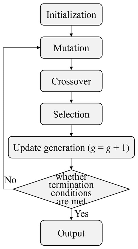
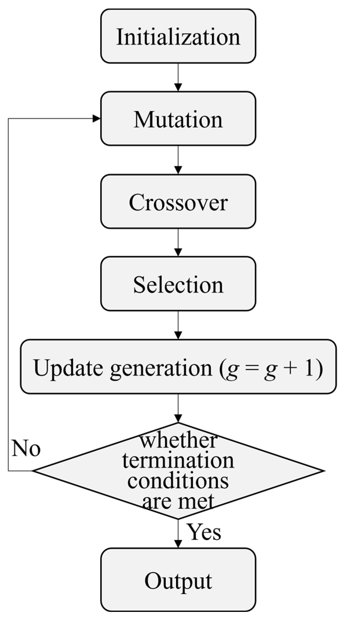
The objective function in this study represents a continuous optimization problem characterized by pronounced nonlinear behavior, which often causes traditional optimization methods to become trapped in local optima, lacking the ability to reliably explore the global search space. To overcome this limitation, a DE algorithm was employed. Differential evolution is a population-based global optimization technique that iteratively improves candidate solutions [45]. The algorithm operates through four fundamental stages: initialization, mutation, crossover, and selection [46]. A schematic representation of the DE algorithm is provided in Figure 4.

Figure 4. Flowchart of the DE algorithm.

3. Results and Discussion

3.1. Overview of Dataset

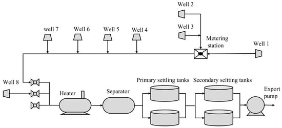
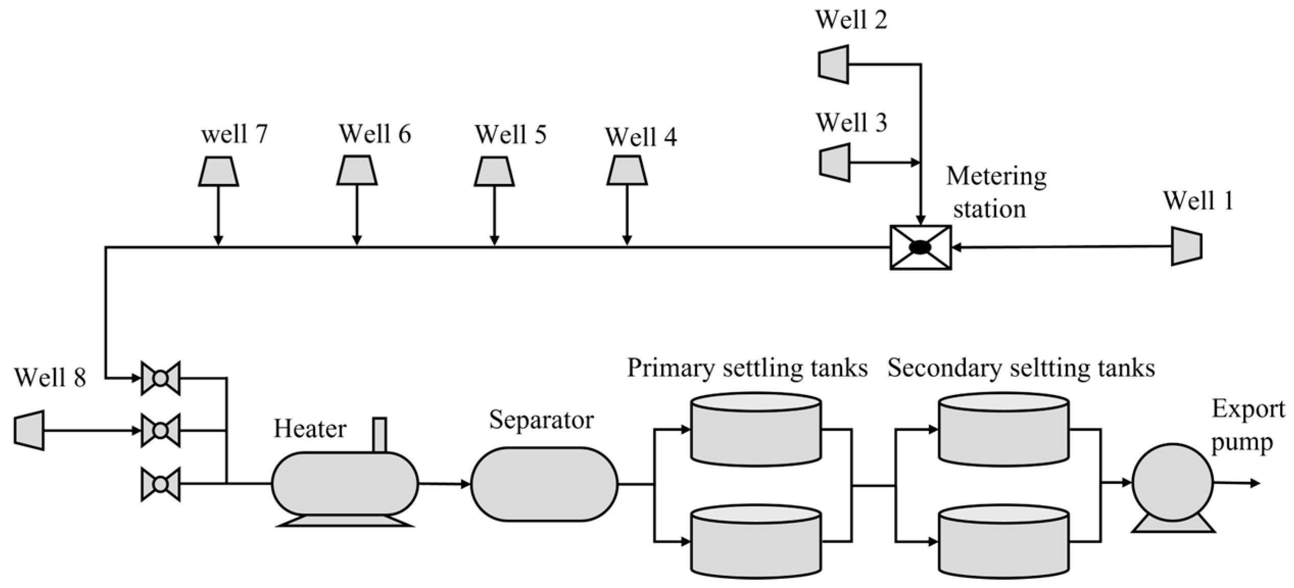
This study focuses on the OGTS located within an oilfield block in China. As illustrated in Figure 5, the OGTS comprises eight wells, one metering station, one heater, one three-phase separator, two primary settling tanks, two secondary settling tanks, and one export pump. Electric heaters are installed at the wellheads of Well 1 and Well 2 to prevent crude oil adhesion to the pipeline walls during transportation, which could otherwise lead to excessive wellhead back pressure.

Figure 5. Production network of the case-study OGTS.

The production command system (PCS) enables real-time acquisition and analysis of operational field data. Authorized users can remotely access historical records and retrieve data at defined sampling intervals, facilitating efficient monitoring and decision-making. In this study, data from the PCS were utilized to develop ANN surrogate models. The dataset encompassed the period from 1 May to 31 May 2025, with measurements recorded at 30 min intervals. This resulted in a total of 1470 data samples for model training and validation. During this period, the OGTS experienced various typical operating conditions, including normal production, equipment start-stop, and production fluctuations. The collected samples possess a high temporal resolution, allowing for a more comprehensive coverage of the system’s main operating states.

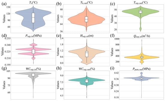
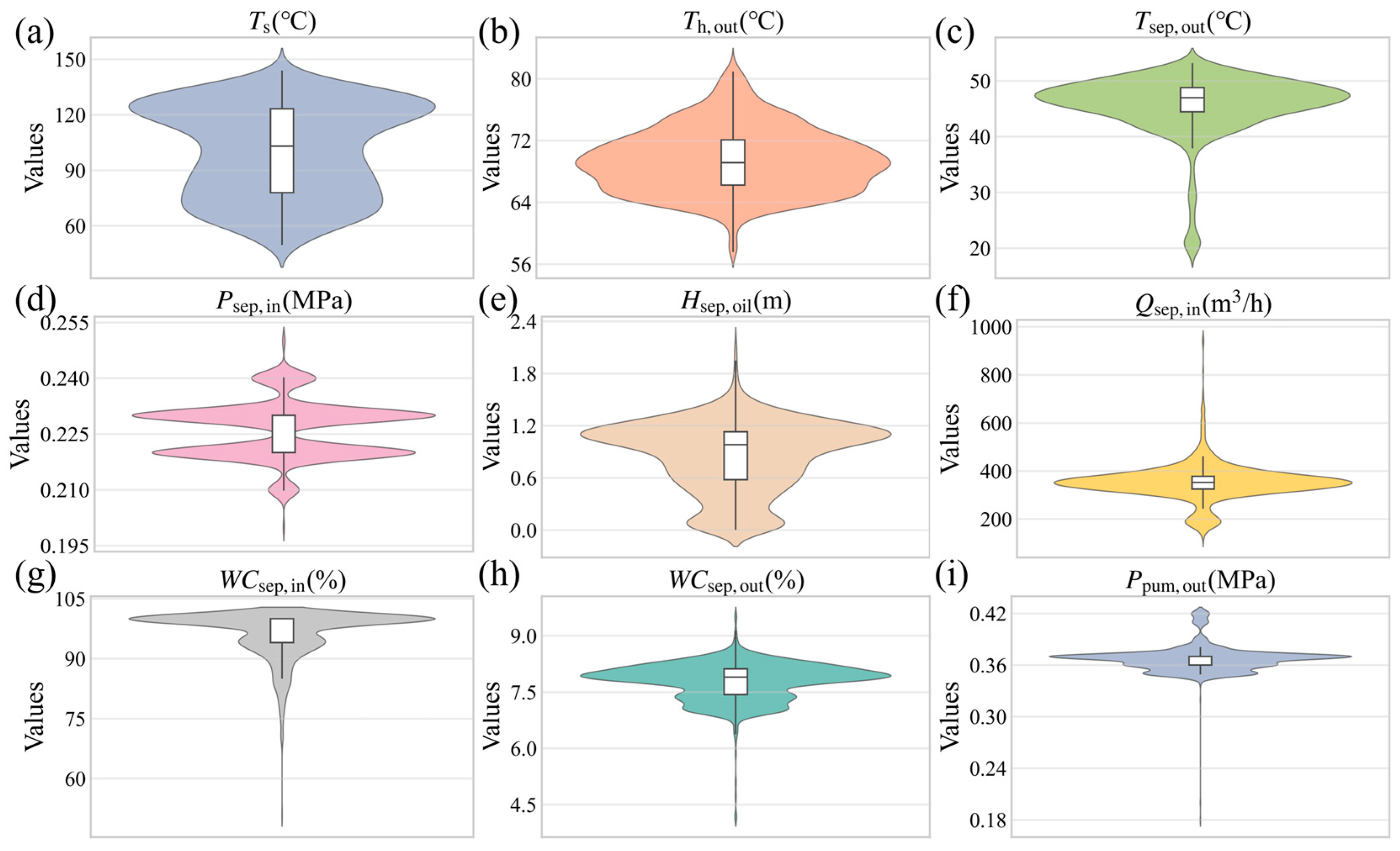
Violin plot and descriptive statistical analyses were performed on selected variables to evaluate data quality and characterize feature distributions. Figure 6 presents violin plots of nine variables for May 2025. The violin plots use Gaussian kernel density estimation to display the probability density distribution of each variable, with wider sections indicating a higher concentration of data points within that value range. Box plots embedded within the violins show statistical features such as the median and interquartile range. As shown in Figure 6a–e, parameters such as flue gas temperature (T_s), heater outlet temperature (T_h,out), separator outlet temperature (T_sep,out), separator inlet pressure (P_sep,in), and oil layer height (H_sep,oil) exhibit typical narrow-peaked distributions. This indicates that these variables are tightly constrained by process design thresholds, with fluctuations generally limited to a small safety range to ensure stable operation of downstream crude oil processing equipment. In contrast, Figure 6f–i display markedly different distribution patterns. The violin plots for separator inlet flow rate (Q_sep,in), inlet water cut (WC_sep,in), and outlet water cut (WC_sep,out) reveal pronounced wide tails and skewed distributions. The wide span of the flow rate distribution directly reflects the natural variability in oilfield inflow. Additionally, the pump outlet pressure (P_pum,out) also demonstrates a relatively broad distribution, which may result from fluctuations in downstream export pressure or variable frequency pump adjustments.

Figure 6. Violin plots illustrating the distributions of selected variables in the dataset for May 2025. (a) flue gas temperature; (b) heater outlet temperature; (c) separator outlet temperature; (d) separator inlet pressure; (e) oil layer level; (f) separator inlet flow rate; (g) separator inlet water cut; (h) separator outlet water cut; (i) pump inlet pressure.

Furthermore, Table 2 presents the mean, standard deviation, range, maximum, minimum, and skewness of each variable in the dataset. These statistics help identify outliers and characterize data distributions, providing a foundation for subsequent artificial neural network model development. As shown in Table 2, the fluctuation characteristics vary significantly among the variables. The flue gas temperature of the heater (T_s) ranges from 49.99 °C to 143.57 °C, reflecting substantial variability in heater operating conditions. In contrast, the heater outlet temperature (T_h,out) varies between 57.66 °C and 81.89 °C with low dispersion, indicating stable outlet temperature control. Additionally, the separator outlet temperature (T_sep,out) and inlet pressure (P_sep,in) exhibit minimal fluctuations, demonstrating consistent system pressure regulation. By comparison, the separator inlet flow rate (Q_sep,in) spans a wide range and has a skewness of 1.35, suggesting that most operating conditions occur at low to medium flow rates. The oil layer level (H_sep,oil) has a skewness of −0.54, indicating a tendency toward generally higher values. Regarding water cut, the separator inlet water cut (WC_sep,in) is relatively high, reflecting the high-water-cut condition of the oilfield block. It is also noted that the separator outlet water cut (WC_sep,out) shows limited variation, with a maximum value of 9.52%, demonstrating effective dehydration performance. Finally, the pump inlet pressure (P_pum,out) ranges from 0.18 MPa to 0.42 MPa, with a skewness of −0.66, indicating that operation is primarily concentrated at higher pressure.

Table 2. Descriptive statistical analysis of selected variables in the dataset.

Statistical Property	Mean	Standard	Range 1	Minimum	Maximum	Skewness
Ts (°C)	100.53	24.88	93.58	49.99	143.57	−0.23
Th,out (°C)	69.43	4.12	24.23	57.66	81.89	0.32
Tsep,out (°C)	45.60	5.63	33.68	19.37	53.05	−2.57
Psep,in (MPa)	0.23	0.01	0.05	0.20	0.25	0.05
Qsep,in (m3/h)	352.74	76.02	822.98	122.97	945.95	1.35
WCsep,in (%)	96.35	5.83	49.00	51.00	100.00	−2.18
Hsep,oil (m)	0.86	0.40	2.12	0.01	2.13	−0.54
WCsep,out (%)	7.78	0.49	5.35	4.17	9.52	−1.43
Ppum,out (MPa)	0.37	0.02	0.24	0.18	0.42	−0.66

¹ The “Range” represents the difference between maximum and minimum values.

It should be noted that highly skewed variables adversely affect the training of the ANN. Skewed distributions typically cause the neural network to focus excessively on data-dense regions while neglecting the sparse tail regions, which may lead to biased predictions and reduce the model’s generalization ability. Additionally, the presence of outliers can cause gradient instability, thereby hindering model convergence. Therefore, before model training, appropriate data preprocessing and outlier handling were implemented. To eliminate the influence of abnormal instances, the interquartile range was used to identify and remove outliers, and Lagrange interpolation was applied to reconstruct the data. Subsequently, to address the issue of different scales and mitigate the adverse effects of skewed distributions, the variables were normalized using min-max scaling to map the data onto the range [0, 1].

3.2. Analysis of Hidden Layer Neurons and Activation Functions

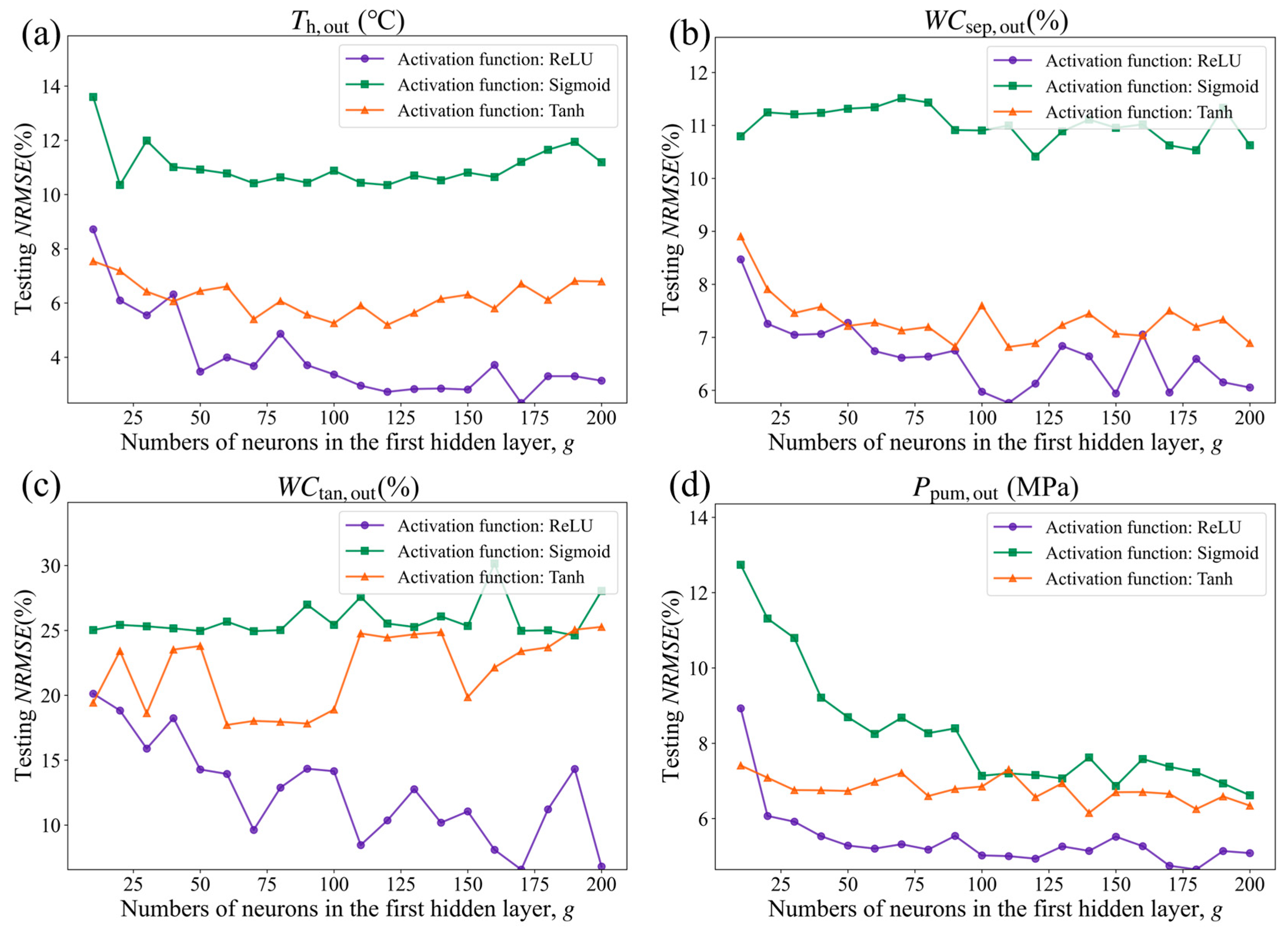
Due to the operational characteristics of different equipment, this study did not adopt a fixed number of hidden layer neurons or a specific activation function [47]. Instead, the network structure was optimized through a series of numerical experiments. The influence of the first hidden layer’s size and the choice of activation function on prediction accuracy was evaluated using NRMSE on the test set. The final surrogate model was selected based on achieving the lowest prediction error while maintaining stable training behavior. The number of neurons in the first hidden layer, denoted as g, was systematically varied within the range of 10 to 200. For each value of g, three activation functions (ReLU, Sigmoid, and Tanh) were tested.

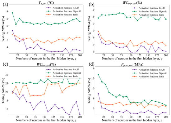
Figure 7 illustrates the variation in NRMSE on the test set as the number of neurons in the first hidden layer increases for different activation functions, with the other hyperparameters held constant. As shown in the figure, networks using the ReLU activation function consistently achieve the lowest NRMSE values across all four subplots. Moreover, the error curves for ReLU are smooth and stable, with minimal fluctuations as the number of neurons increases. In contrast, networks employing Sigmoid and Tanh activation functions generally exhibit higher errors, and as network size grows, the error curves display pronounced oscillations, particularly in water cut prediction. This can be attributed to the saturation of gradients in Sigmoid and Tanh functions, which tend to cause gradient saturation, resulting in reduced model generalization. Sensitivity analysis with respect to neuron count reveals that for the ReLU model, NRMSE decreases rapidly as the number of neurons increases from 10 to 50, stabilizes between 50 and 100, and shows diminishing returns or potential overfitting beyond 150 neurons. For Sigmoid and Tanh models, the error is more sensitive to the number of neurons; optimal performance typically occurs with smaller network sizes, while larger networks actually lead to degraded performance. Based on this analysis, this study selects 50 neurons and the ReLU activation function for the first hidden layer as the optimal BPNN configuration. Considering the marginal returns of computational resources, 50 neurons represent the critical inflection point for error convergence, beyond which increasing the number of nodes no longer brings significant improvements in accuracy.

Figure 7. Test-set NRMSE as a function of the number of neurons in the first hidden layer for different activation functions: (a) heater outlet temperature, (b) water cut at the separator outlet, (c) water cut at the settling tank outlet, (d) export pump outlet pressure.

3.3. Prediction Performance Analysis of the Models

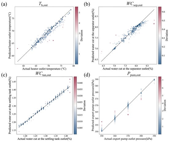
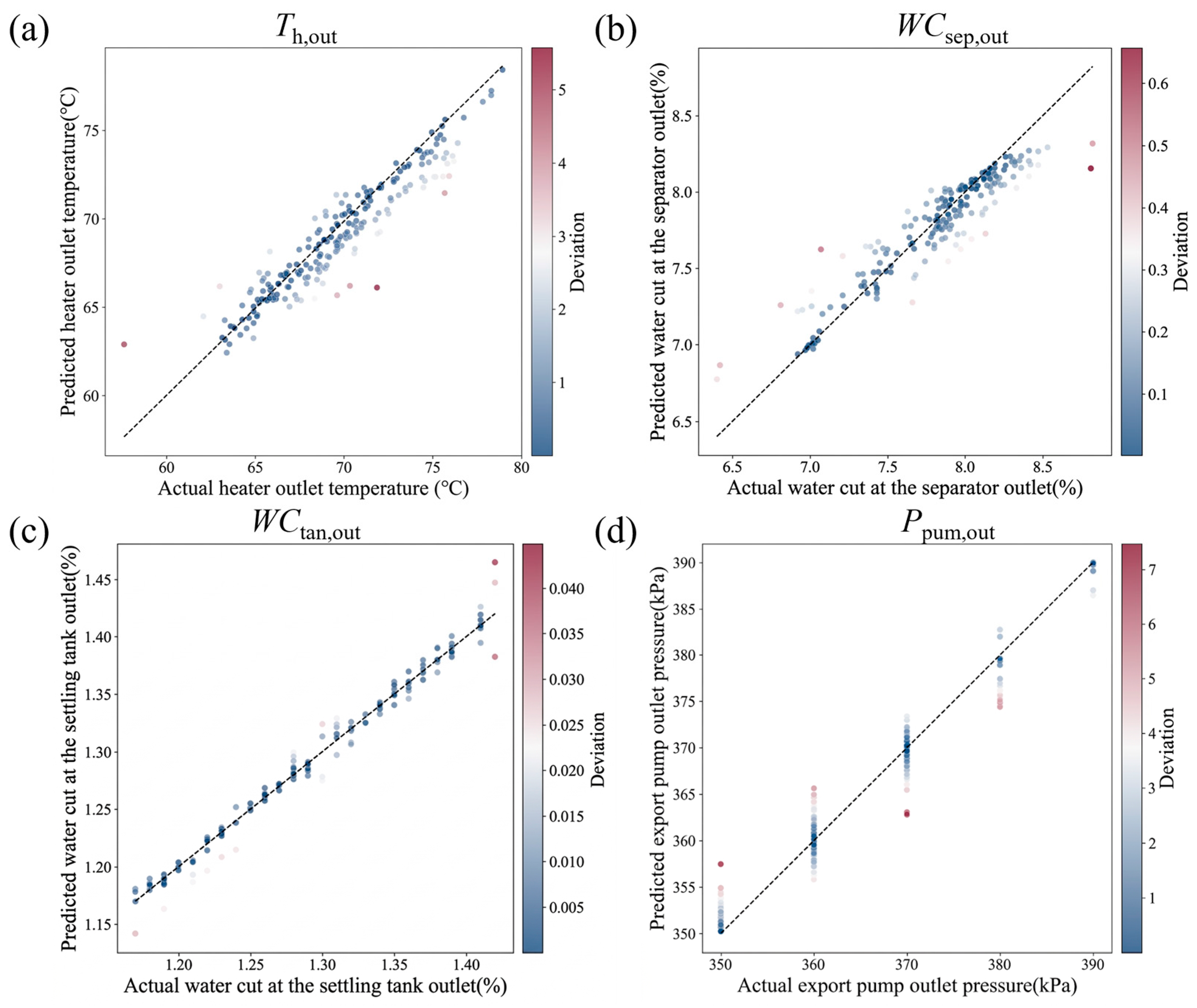
Figure 8 shows the comparison between the predicted and actual values of the four key output variables generated by the surrogate model. As illustrated in Figure 8a,b, the prediction points for the heater outlet temperature and the separator outlet water cut are closely clustered around the ideal diagonal, indicating high prediction accuracy for these two variables. In contrast, Figure 8c,d display a relatively higher degree of dispersion for the settling tank outlet water cut and the export pump outlet pressure. This phenomenon can be attributed to the limitations of data-driven models when handling low signal-to-noise ratios and discrete measurement data [48]. The actual ranges of water content and pressure data are relatively narrow, and extremely small target variances can significantly amplify the impact of inherent measurement noise. Additionally, the data points exhibit a vertically banded distribution, indicating that the on-site measurement instruments have limited resolution, which introduces systematic quantization errors. When the smooth and continuous outputs of the surrogate model are compared with these low-resolution, discrete ground-truth values, pronounced dispersion inevitably appears in the scatter plots.

Figure 8. Comparison of actual and predicted values from the developed surrogate models: (a) heater outlet temperature, (b) water cut at the separator outlet, (c) water cut at the settling tank outlet, (d) export pump outlet pressure. The dashed lines represent the ideal prediction line.

Table 3 summarizes the performance metrics of the surrogate models developed on the test dataset: R², RMSE, NRMSE, and MAE. The results indicate that the ANN-based prediction models for key equipment exhibit overall high accuracy, with all models achieving R² values above 0.85. This demonstrates that the models can effectively capture the nonlinear relationships between system inputs and outputs. Among all models, the prediction model for the water cut at the outlet of the settling tank performed the best, achieving an R² of 0.929 on the test dataset, with corresponding RMSE, NRMSE, and MAE values of 0.013, 4.25, and 0.01, respectively. In addition, the R² values of all models range from 0.854 to 0.979, and the RMSE values range from 4.25 to 6.67, indicating low prediction errors and high model stability, which provide a robust and reliable representation of system states for subsequent optimization calculations.

Table 3. Performance metrics of the developed surrogate models.

Surrogate Models	R2	RMSE	NRMSE	MAE
Th,out (°C)	0.889	1.14	5.69	1.03
WCsep,out (%)	0.854	0.17	6.67	0.12
WCtan,out (%)	0.979	0.013	4.25	0.01
Ppum,out (kPa)	0.946	2.27	5.68	1.73

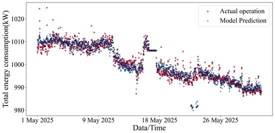
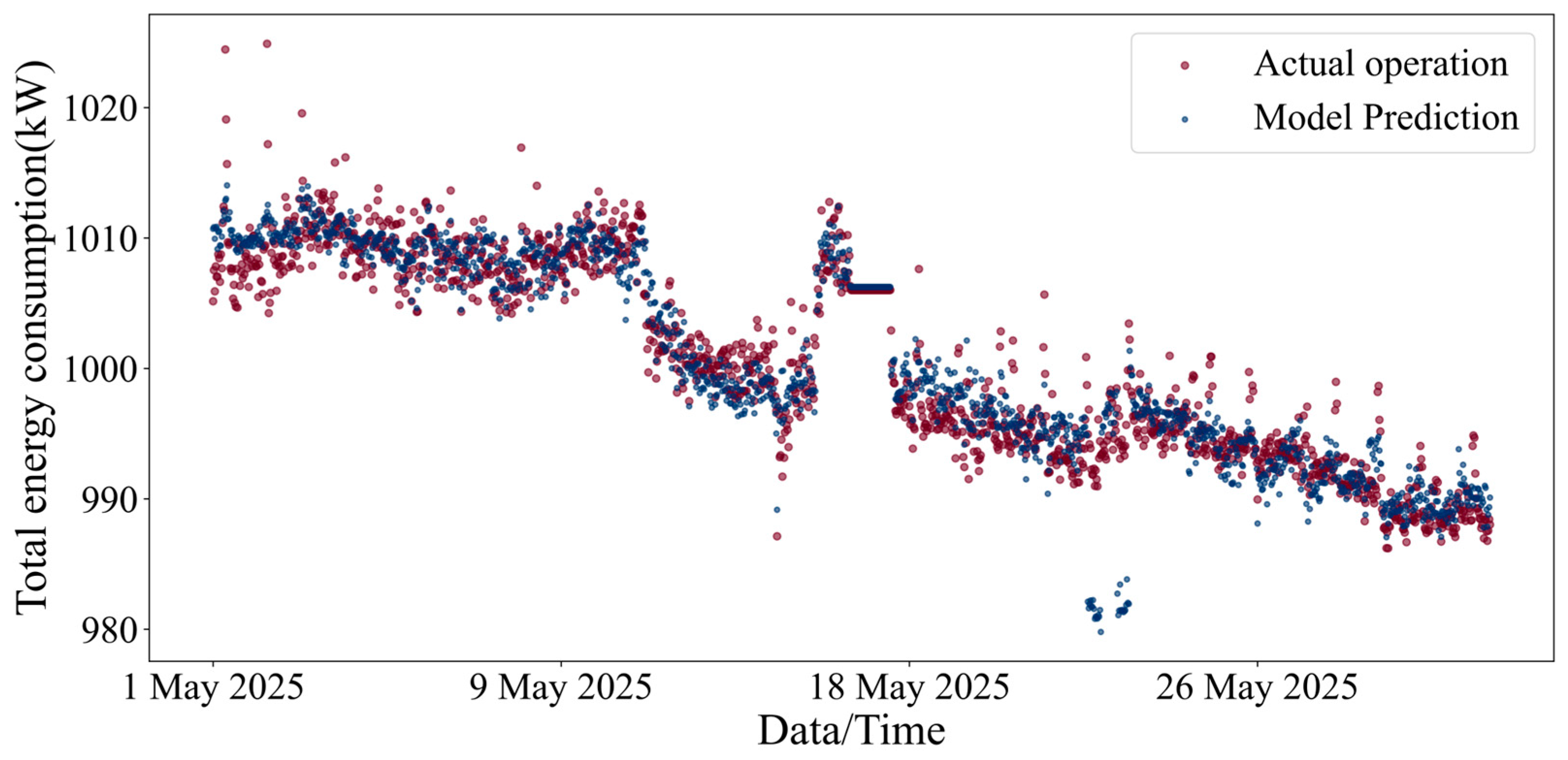
Based on the developed surrogate models and the process flow, an OGTS surrogate model was established to predict the overall operating state. The surrogate model was then rigorously validated, with particular focus on total system energy consumption, the primary prediction target. Figure 9 presents a time-series comparison between the total energy consumption predicted by the surrogate model and the actual operating data. The blue solid line represents the actual values, while the red dashed line indicates the model predictions. As shown in Figure 9, the predicted curve closely tracks the variations and fluctuation amplitudes of the measured data throughout the study period. The deviations between them are minor, with no apparent accumulation of error, demonstrating the model’s strong dynamic response capability. Notably, the prediction errors primarily occur during periods of significant energy consumption fluctuations, whereas during phases of relatively stable system operation, the model achieves almost unbiased predictions. This phenomenon may be related to information transmission delays of input variables under dynamic conditions or the amplification of measurement noise. The NRMSE can eliminate the influence of variable dimensions, facilitating fair comparisons across datasets with different scales [44,49]. The NRMSE of the prediction results is 7.74%, which is slightly higher than those of the four operating parameter models in Table 3, mainly due to error propagation effects. The mean absolute percentage error of the prediction results is 3.41%, which is at a relatively low level.

Figure 9. Comparison between actual operational data and surrogate model predictions of total energy consumption.

3.4. Optimization Results

Using the developed OGTS surrogate model, the optimization problem was solved by applying a DE algorithm to search for the global optimum. Table 4 summarizes the results of a single optimization with a 30 min interval, including the optimized process variables and the corresponding total energy consumption. The inlet heating temperature of Pipeline 1 was reduced from 29.3 °C to 25.6 °C, while that of Pipeline 2 decreased from 33.26 °C to 29.75 °C. The heater outlet temperature was lowered from 65.8 °C to 63.28 °C, suggesting that the optimization strategy prioritizes a moderate reduction in heating intensity to minimize thermal energy input while still satisfying dehydration and transportation requirements. In terms of dehydration performance, the outlet water cuts of the separator and settling tanks increased slightly due to the reduced temperatures. However, all values remained within acceptable operational limits, confirming the feasibility and engineering applicability of the optimization outcomes. Overall, the total energy consumption of the OGTS was reduced by approximately 2.28%, and the optimization algorithm completed in under 3 min, demonstrating both efficiency and practical applicability.

Table 4. Optimized process variables and corresponding total energy consumption for the OGTS.

Optimized Parameters	Actual	Optimization Model
Heating temperature at the pipeline inlet (°C)	29.3	25.6
Heating temperature at the Heater (°C)	65.8	63.28
Water cut at the separator outlet (%)	8.10	8.15
Water cut at the settling tank outlet (%)	1.18	1.16
Total energy consumption, FEC (kW)	1002.3	979.4

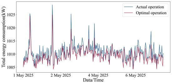
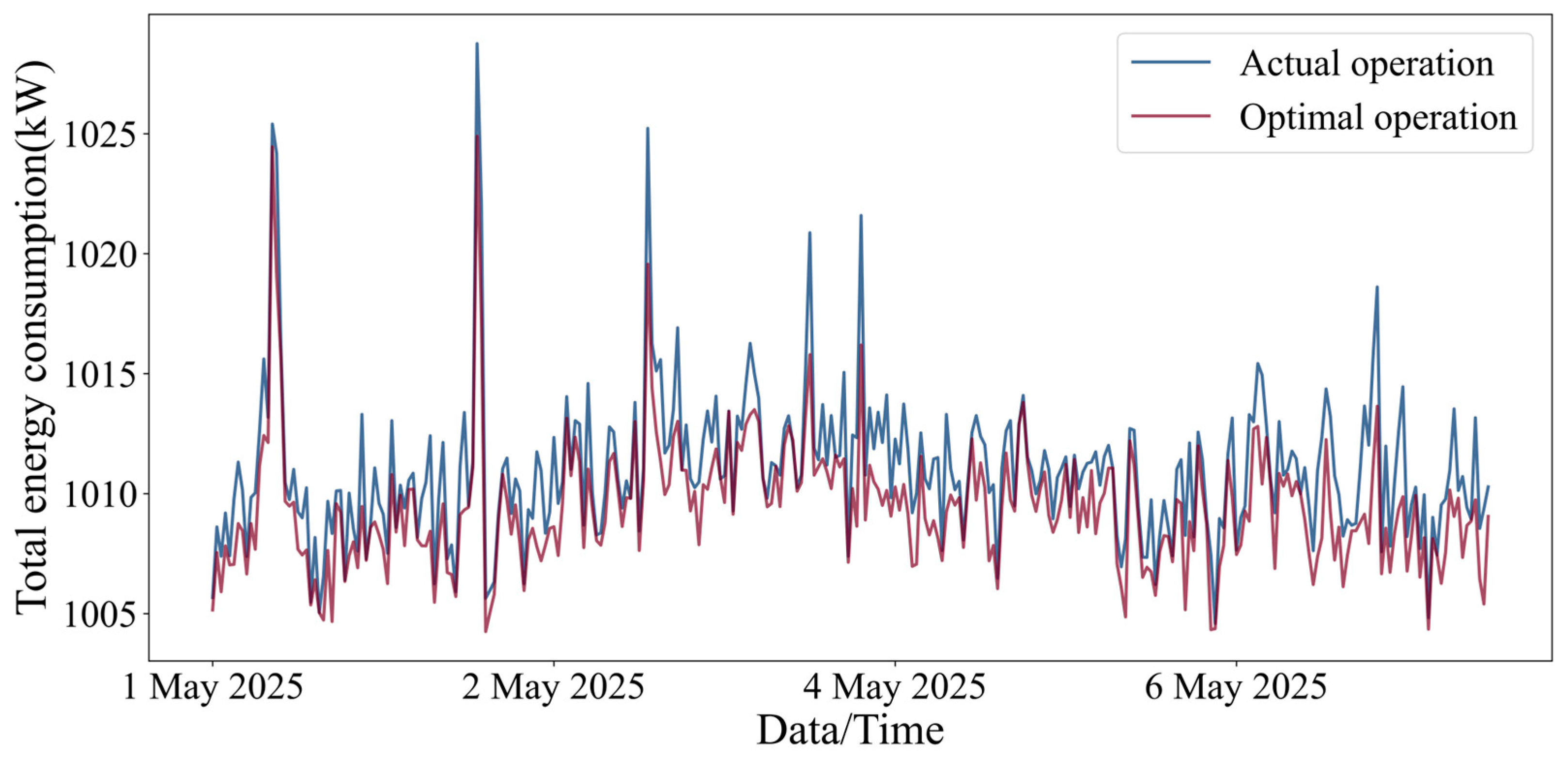
In contrast to Table 4, which presents the result of a single optimization run, Figure 10 summarizes the results from multiple optimization runs. The energy-saving effects range from 0% to 5.66%. In addition, Figure 10 compares the daily total energy consumption under actual operating conditions and optimized operating conditions over the selected time period. The blue bars represent actual values, while the orange bars represent optimized values. As shown in Figure 10, the optimized energy consumption trajectory never significantly exceeds the actual operating values on any date, and the trend of optimized energy consumption closely matches that of the actual operating conditions. Notably, the energy consumption peaks observed during actual operations are effectively suppressed in the optimized scenario. For example, on 2 May, the actual energy consumption peak of 1028.75 kW was reduced to 1024.89 kW after optimization, with no further increase, demonstrating the effectiveness of the optimization model’s capability to mitigate unfavorable operating conditions. Statistical analysis indicates that, over the selected time period, the optimized system’s average daily energy consumption was reduced by approximately 1.55% compared to actual operation, further verifying the stability and effectiveness of the proposed optimization method in reducing overall system energy consumption. Although the energy-saving effect after optimization is not significant, the direct economic benefits accumulated over long-term operation remain highly significant given the large energy consumption of the OGTS. In addition, the study’s effective suppression of energy consumption peaks helps prevent core equipment such as heaters and pumps from operating inefficiently under high-load conditions. This not only reduces electricity costs in oilfields with peak-valley electricity pricing policies but also effectively alleviates equipment load during operation, extends service life, and significantly enhances the overall reliability and safety of the OGTS in long-term operation.

Figure 10. Comparison of daily total energy consumption under actual operation versus optimal operation.

4. Conclusions

An operation optimization study based on ANN surrogate models was conducted to determine the optimal coordinated operation strategy for the pipeline network and processing station. This study established an integrated optimization framework, validated using production data from the OGTS in a domestic oilfield block. The key conclusions of this study are summarized as follows:

(1)

Numerical experiments have determined that the ANN model achieves optimal predictive performance when using the ReLU activation function and configuring 50 neurons in the first hidden layer. This indicates that the architecture can accurately capture the complex nonlinear thermodynamic and dynamic characteristics of the OGTS, achieving an optimal balance between model convergence speed and computational complexity. All developed ANN surrogate models achieved R² values above 0.85 on the test set, with R² values as high as 0.979. This high level of fitting accuracy fully validates the robustness and feasibility of using neural network methods to construct nonlinear surrogate models and meets the engineering accuracy requirements for process parameter prediction in oilfield operations.

(2)

During a single 30 min optimization cycle, the total energy consumption of the OGTS was reduced by 2.28%, and the DE algorithm completed the computation within 3 min. This result demonstrates the timeliness of the optimization framework in handling single-condition adjustments, providing technical support for real-time optimization control in the OGTS.

(3)

According to statistical analysis of the full month’s operational data, the average daily energy-saving rate of the OGTS was 1.55%, with a peak energy-saving rate reaching 5.66%, fully confirming the robustness of the optimization strategy in dynamic and complex operating conditions. This optimization framework significantly reduces the load and fatigue stress on core equipment by smoothing energy consumption peaks, which is of great practical significance for extending equipment service life and improving the overall economic benefits of oilfield operations.

Future research may incorporate operational data spanning multiple months and years, combined with incremental learning or transfer learning methods, to further enhance the temporal generalization capability of the surrogate model.

References

- Liu, X.; Peng, R.; Bai, C.; Chi, Y.; Liu, Y. Economic cost, energy transition, and pollutant mitigation: The effect of China’s different mitigation pathways toward carbon neutrality. Energy 2023, 275, 127529. [Google Scholar] [CrossRef] [Scilit]
- Salim, S.S.; Luxembourg, S.L.; Smekens, K.; Dalla Longa, F.; van der Zwaan, B. Pathways to climate neutrality: Europe’s energy transition under the Green Deal. Renew. Sustain. Energy Rev. 2026, 226, 116272. [Google Scholar] [CrossRef] [Scilit]
- Zhang, X.; Hou, L.; Liu, J.; Yang, K.; Chai, C.; Li, Y.; He, S. Energy consumption prediction for crude oil pipelines based on integrating mechanism analysis and data mining. Energy 2022, 254, 124382. [Google Scholar] [CrossRef] [Scilit]
- Chen, J.; Wang, W.; Sun, W.-Y.; Li, D.; Jiao, Y.-B. Oilfield sustainability and management: An optimization model for the reconstruction of oil and gas gathering systems based on potential location mining. Pet. Sci. 2025, 22, 935–955. [Google Scholar] [CrossRef] [Scilit]
- Xiong, X.; Xu, N.; Xing, X.; Xue, R.; Li, Y. Design of intelligent scheduling and optimization decision system for multi-source regional crude oil transportation and distribution system. Int. Commun. Heat Mass Transf. 2025, 164, 108881. [Google Scholar] [CrossRef] [Scilit]
- Liu, Y.; Cheng, Q.; Gan, Y.; Wang, Y.; Li, Z.; Zhao, J. Multi-objective optimization of energy consumption in crude oil pipeline transportation system operation based on exergy loss analysis. Neurocomputing 2019, 332, 100–110. [Google Scholar] [CrossRef] [Scilit]
- Pan, S.; Zhao, H.; Li, H.; Geng, Y.; Du, J.; Li, Z.; Niu, P.; Zhang, Z.; Yan, F.; Xu, N.; et al. An MILP model for the coupled design and operation optimization of large-scale gathering pipeline networks. J. Pipeline Sci. Eng. 2025, 5, 100359. [Google Scholar] [CrossRef] [Scilit]
- Zhang, X.-Q.; Cheng, Q.-L.; Sun, W.; Zhao, Y.; Li, Z.-M. Research on a TOPSIS energy efficiency evaluation system for crude oil gathering and transportation systems based on a GA-BP neural network. Pet. Sci. 2024, 21, 621–640. [Google Scholar] [CrossRef] [Scilit]
- Zhao, Y.; Yao, L.; Liu, L.; Xu, Y. Optimization of energy saving gathering and transportation mode in a block of Tahe oilfield. Case Stud. Therm. Eng. 2019, 13, 100378. [Google Scholar] [CrossRef] [Scilit]
- Zhou, J.; He, Y.; Chen, Y.; Zhou, L.; Liu, S.; Li, H.; Liang, G. A novel optimization model for tackling capacity challenges in natural gas gathering systems. Energy 2024, 305, 132377. [Google Scholar] [CrossRef] [Scilit]
- Dhandhi, Y.; Chaudhari, R.K.; Naiya, T.K. Development in separation of oilfield emulsion toward green technology—A comprehensive review. Sep. Sci. Technol. 2022, 57, 1642–1668. [Google Scholar] [CrossRef] [Scilit]
- Song, C.; Guo, W.; Gao, X.; Li, Q.; He, H.; Chi, M. Molecular dynamics approach to interfacial manipulation and dehydration enhancement of crude oil emulsions: A case study on plasma pre-treatment. RSC Adv. 2025, 15, 45014–45025. [Google Scholar] [CrossRef] [Scilit] [PubMed]
- Zolfaghari, R.; Fakhru’l-Razi, A.; Abdullah, L.C.; Elnashaie, S.S.E.H.; Pendashteh, A. Demulsification techniques of water-in-oil and oil-in-water emulsions in petroleum industry. Sep. Purif. Technol. 2016, 170, 377–407. [Google Scholar] [CrossRef] [Scilit]
- Trevisan, L.; Shokry, A.; Montini, M.; Moulines, E.; Zio, E. A hybrid approach for steady-state production optimization of a real oil and gas platform: Integrating physics-based models, machine learning techniques, and field monitoring signals. Comput. Chem. Eng. 2025, 203, 109320. [Google Scholar] [CrossRef] [Scilit]
- Chen, J.; Wang, W.; Sun, W.; Chen, J.; Wang, Q.; Li, T. Oilfield sustainable development: An operation optimization study for the water-flooding pipeline network system based on data fusion. J. Clean. Prod. 2025, 518, 145866. [Google Scholar] [CrossRef] [Scilit]
- Li, H.; Fan, T.; Wang, K.; Long, X.; He, Y.; Wang, M.; Cheng, W.; Huang, Q.; Huang, H.; Yu, W. An optimal flow rate allocation model of the oilfield treated oil pipeline network. Petroleum 2024, 10, 93–100. [Google Scholar] [CrossRef] [Scilit]
- Ríos-Mercado, R.Z.; Borraz-Sánchez, C. Optimization problems in natural gas transportation systems: A state-of-the-art review. Appl. Energy 2015, 147, 536–555. [Google Scholar] [CrossRef] [Scilit]
- Liu, E.; Lai, P.; Peng, Y.; Chen, Q. Research on optimization operation technology of QT oil pipeline based on the Heuristic algorithm. Energy Rep. 2022, 8, 10134–10143. [Google Scholar] [CrossRef] [Scilit]
- Wei, X.; Qiu, R.; Zhang, B.; Liu, C.; Wang, G.; Wang, B.; Liang, Y. Operation optimization of large-scale natural gas pipeline networks based on intelligent algorithm. Energy 2024, 310, 133258. [Google Scholar] [CrossRef] [Scilit]
- Chen, S.; Lyu, Y.; Li, H. Optimization of production and operation parameters of oil field gathering and transportation system. Oil Gas Storage Transp. 2020, 39, 418–424. [Google Scholar]
- Kashani, M.; Jespersen, S.; Yang, Z. Oil-in-water concentration prediction for offshore oil & gas produced water treatment using deep learning approach with hyperparameter optimization. Energy Rep. 2025, 14, 4275–4290. [Google Scholar] [CrossRef] [Scilit]
- Otte Hülse, E.; Lima Silva, T.; Camponogara, E.; Ramos Rosa, V.; Ferreira Vieira, B.; Furtado Teixeira, A. Introducing approximate well dynamics into production optimization for operations scheduling. Comput. Chem. Eng. 2020, 136, 106773. [Google Scholar] [CrossRef] [Scilit]
- Rostamian, A.; de Moraes, M.B.; Schiozer, D.J.; Coelho, G.P. A survey on multi-objective, model-based, oil and gas field development optimization: Current status and future directions. Pet. Sci. 2025, 22, 508–526. [Google Scholar] [CrossRef] [Scilit]
- Ghafariasl, P.; Mahmoudan, A.; Mohammadi, M.; Nazarparvar, A.; Hoseinzadeh, S.; Fathali, M.; Chang, S.; Zeinalnezhad, M.; Garcia, D.A. Neural network-based surrogate modeling and optimization of a multigeneration system. Appl. Energy 2024, 364, 123130. [Google Scholar] [CrossRef] [Scilit]
- Hoffmann, A.; Stanko, M. Short-term model-based production optimization of a surface production network with electric submersible pumps using piecewise-linear functions. J. Pet. Sci. Eng. 2017, 158, 570–584. [Google Scholar] [CrossRef] [Scilit]
- Das, S.; Suganthan, P.N. Differential Evolution: A Survey of the State-of-the-Art. IEEE Trans. Evol. Comput. 2011, 15, 4–31. [Google Scholar] [CrossRef] [Scilit]
- Mohammadi, A.; Sheikholeslam, F. Intelligent optimization: Literature review and state-of-the-art algorithms (1965–2022). Eng. Appl. Artif. Intell. 2023, 126, 106959. [Google Scholar] [CrossRef] [Scilit]
- Dai, C.; Sun, X.; Zhang, Y.; Gong, D. Multiform optimization with coupled subspace alignment and two-stage adaptive differential evolution for interval constrained scheduling of coal mine integrated energy systems. Swarm Evol. Comput. 2026, 100, 102256. [Google Scholar] [CrossRef] [Scilit]
- Koyuncuoğlu, M.U. Sustainable configuration of production lines: Multi-objective energy-efficient optimization with adaptive differential evolution and golden ratio algorithms. Eng. Appl. Artif. Intell. 2026, 165, 113469. [Google Scholar] [CrossRef] [Scilit]
- Tian, W.; Qu, J.; Liu, B.; Cui, Z.; Hu, M. Parameter prediction of oilfield gathering station reservoir based on feature selection and long short-term memory network. Measurement 2023, 206, 112317. [Google Scholar] [CrossRef] [Scilit]
- Wang, X.; Ji, W. Data-driven robust topology optimization using surrogate modeling, model reduction, and machine learning. Eng. Appl. Artif. Intell. 2026, 163, 113136. [Google Scholar] [CrossRef] [Scilit]
- Yin, X.; Wen, K.; Wu, Y.; Han, X.; Mukhtar, Y.; Gong, J. A machine learning-based surrogate model for the rapid control of piping flow: Application to a natural gas flowmeter calibration system. J. Nat. Gas Sci. Eng. 2022, 98, 104384. [Google Scholar] [CrossRef] [Scilit]
- Bocoum, A.O.; Rasaei, M.R. Multi-objective optimization of WAG injection using machine learning and data-driven Proxy models. Appl. Energy 2023, 349, 121593. [Google Scholar] [CrossRef] [Scilit]
- Wu, J.; Zhang, L.; Liang, W.; Hu, J. A novel failure mode analysis model for gathering system based on Multilevel Flow Modeling and HAZOP. Process Saf. Environ. Prot. 2013, 91, 54–60. [Google Scholar] [CrossRef] [Scilit]
- García Kerdan, I.; Morillón Gálvez, D. Artificial neural network structure optimisation for accurately prediction of exergy, comfort and life cycle cost performance of a low energy building. Appl. Energy 2020, 280, 115862. [Google Scholar] [CrossRef] [Scilit]
- Luo, X.; Hu, Z.; Zhang, Q.; Pang, Y. Recent development in thermodynamic prediction of oilfield scale: From mechanistic models to machine learning. Sustain. Energy Technol. Assess. 2025, 84, 104744. [Google Scholar] [CrossRef] [Scilit]
- Matijošius, J.; Rimkus, A.; Gruodis, A.; Chiavola, O.; Recco, E. Simulation of Diesel Engine Properties Using Different Mixtures of Fuels by Means of a Feed-Forward Neural Network: 1. Validation and Prediction of Energetical Parameters. Energies 2026, 19, 888. [Google Scholar] [CrossRef] [Scilit]
- Ricci, M.; Gianaroli, F.; Artioli, M.; Beozzo, S.; Sdringola, P. Multi-Step Artificial Neural Networks for Predicting Thermal Prosumer Energy Feed-In into District Heating Networks. Energies 2025, 18, 6608. [Google Scholar] [CrossRef] [Scilit]
- Sun, P.; Zhang, J.; Dong, W.; Li, D.; Yu, X. Prediction of oxygen-enriched combustion and emission performance on a spark ignition engine using artificial neural networks. Appl. Energy 2023, 348, 121466. [Google Scholar] [CrossRef] [Scilit]
- Yang, Z.; Yang, J.; Sun, H.; Liu, W.; Li, H.; Zhu, Q. Integrating multiphysics modeling and machine learning for enhanced efficiency and thermal management in PEM water electrolyzer systems. Appl. Energy 2025, 401, 126613. [Google Scholar] [CrossRef] [Scilit]
- Mafat, I.H.; Palla, S.; Ambati, S.R.; Narayana, R.; Girish Kumar, K.V.; Swaroop, G.J. Data-driven modeling of bio-oil yield in agricultural biomass pyrolysis with machine learning. Int. J. Hydrogen Energy 2025, 137, 1248–1259. [Google Scholar] [CrossRef] [Scilit]
- Mahjoubi, S.; Meng, W.; Bao, Y. Auto-tune learning framework for prediction of flowability, mechanical properties, and porosity of ultra-high-performance concrete (UHPC). Appl. Soft Comput. 2022, 115, 108182. [Google Scholar] [CrossRef] [Scilit]
- Dastranj, M.; Sepaskhah, A.R. Modelling perennial saffron growth and yield under different irrigation water salinities, irrigation water levels and planting methods. Agric. Water Manag. 2026, 323, 110097. [Google Scholar] [CrossRef] [Scilit]
- Rabbi, M.F. Cross-framework hybrid artificial intelligence for high-penetration renewable energy integration: Multi-regional forecasting and adaptive control. Appl. Energy 2025, 401, 126834. [Google Scholar] [CrossRef] [Scilit]
- Cheng, L.; Li, Y.; Wang, J.; Ma, C.; Zhan, X. Prediction of laser welding deformation using a deep learning model optimized by a differential evolution algorithm. Chin. J. Mech. Eng. 2026, 39, 100083. [Google Scholar] [CrossRef] [Scilit]
- Wang, L.; Yao, Y.; Luo, X.; Daniel Adenutsi, C.; Zhao, G.; Lai, F. A critical review on intelligent optimization algorithms and surrogate models for conventional and unconventional reservoir production optimization. Fuel 2023, 350, 128826. [Google Scholar] [CrossRef] [Scilit]
- Wang, C.; Zhang, H.; Xie, L.; Zhu, C.; Jin, Z.; Hu, X.; Zhang, T.; Cai, G.; Liu, S. ANN-based prediction of compressive strength in sustainable HPC using industrial waste. Constr. Build. Mater. 2025, 505, 144780. [Google Scholar] [CrossRef] [Scilit]
- Harish, A.; Prince, A.; Jayan, M.V. Fault Detection and Classification for Wide Area Backup Protection of Power Transmission Lines Using Weighted Extreme Learning Machine. IEEE Access 2022, 10, 82407–82417. [Google Scholar] [CrossRef] [Scilit]
- Musbah, H.; Elsaraiti, M. Forecasting load consumption: A comprehensive evaluation of deep learning and machine learning techniques. Electr. Power Syst. Res. 2025, 247, 111834. [Google Scholar] [CrossRef] [Scilit]
Disclaimer/Publisher’s Note: The statements, opinions and data contained in all publications are solely those of the individual author(s) and contributor(s) and not of MDPI and/or the editor(s). MDPI and/or the editor(s) disclaim responsibility for any injury to people or property resulting from any ideas, methods, instructions or products referred to in the content. |
© 2026 by the authors. Licensee MDPI, Basel, Switzerland. This article is an open access article distributed under the terms and conditions of the Creative Commons Attribution (CC BY) license.