


Abstract
The widespread use of gasoline blended with 10% ethanol (E10) has raised questions regarding engine performance and emissions under conditions where ethanol supply may be disrupted, and pure gasoline (E0) is temporarily used instead. This study experimentally investigates the effects of E0 and E10 fuels on fuel consumption and exhaust emissions in spark-ignition engines equipped with two different fuel supply systems: multi-point fuel injection (MPI) and carburetion (CARB). Chassis dynamometer tests were performed on two passenger vehicles under steady-state part-load conditions at vehicle speeds of 60, 90, and 120 km/h, as well as during full-throttle operation. E0 and E10 were tested separately under identical operating points. Fuel consumption, brake-specific fuel consumption, air–fuel ratio, and exhaust gas components (CO, CO2, HC, O2) were measured and analysed. The results show that the MPI-equipped vehicle exhibited consistently lower fuel consumption when operating on E0 compared to E10, primarily due to the lower volumetric heating value of ethanol. In contrast, the carbureted engine demonstrated a stronger sensitivity to fuel composition, with E10 leading to leaner mixture formation and pronounced changes in fuel consumption and emissions. CO and HC emissions were significantly lower in the MPI engine, mainly due to closed-loop stoichiometric control combined with the presence of a three-way catalytic converter, while E10 substantially reduced these emissions in the carbureted engine. CO and HC emissions were significantly lower in the MPI configuration, mainly due to closed-loop stoichiometric control combined with the presence of a three-way catalytic converter. In the carbureted configuration, E10 substantially reduced CO and HC emissions compared to E0, primarily as a result of leaner mixture formation. Overall, the findings indicate that modern MPI engines are less sensitive to whether the supplied fuel is E10 and E0, whereas carbureted engines may show notable changes in performance and emissions under the same operating conditions.
1. Introduction
Global energy demand continues to increase, while fossil fuels and other non-renewable energy resources are being progressively depleted [1,2]. Consequently, it is essential to use the remaining reserves more rationally and efficiently, and to further explore alternative energy sources. In the transport sector, reducing the consumption of petroleum-based fuels is a primary objective, particularly for oil-importing countries. Decreasing the use of such fuels in internal combustion engines would also directly contribute to improving environmental conditions, especially in densely populated urban areas [3,4].
One of the most promising strategies to reduce petroleum-based fuel consumption in transportation is the substitution of conventional fuels with alternative or renewable energy sources [5]. Over recent decades, various measures have been implemented to reduce greenhouse gas (GHG) emissions, with bioethanol–gasoline blending remaining one of the most widely adopted solutions [6].
However, the application of bioethanol is constrained by its hygroscopic nature. Phase separation may occur at water concentrations as low as 0.5% by volume when condensation droplets enter the fuel tank [7]. As water content increases, the lower heating value of the blend decreases and combustion slows, leading to reduced thermal efficiency, higher specific fuel consumption, and elevated CO and HC emissions prior to catalytic conversion. These effects are associated with poorer mixture oxidation and prolonged ignition delay [6].
Several studies have demonstrated that adding biofuels such as ethanol or butanol to gasoline can improve engine performance, particularly in carbureted engines. For example, a 10% bioethanol blend has been reported to increase efficiency by approximately 6%, while a 20% butanol blend may achieve improvement of up to 8% [8]. Thus, biofuel blends can be considered potentially beneficial for the combustion process.
Nevertheless, ethanol addition increases fuel vapour pressure and the risk of phase separation. Ethanol derivatives such as ethyl tertiary-butyl ether (ETBE) offer improved storage stability and help reduce ethanol losses in the presence of water [7]. Increased water content also slows combustion, necessitating adjustments to ignition timing and the air–fuel ratio under varying operating conditions [9].
In modern fuel injection engines, ethanol–gasoline blends typically reduce CO and HC emissions due to the higher oxygen content, which promotes more complete combustion. The most significant reductions are generally observed at ethanol concentrations around 20%. However, under low ambient temperatures or at high ethanol content, CO and HC emissions may increase due to reduced fuel volatility and lower flame temperatures [10].
While E15 blends can reduce CO and certain other pollutants, they may also increase acetaldehyde emissions [11]. E20 fuel exhibits properties similar to gasoline, and long-term durability studies indicate minimal impact on fuel consumption or major emissions. However, due to its lower heating value, E20 may increase CO2 and HC emissions, although NOx emissions tend to decrease [12]. E10 fuel has also been found to reduce CO and HC emissions, while increasing the formation of oxygenated compounds, particularly acetaldehyde [13].
Additional studies conducted under the Federal Test Procedure have confirmed that E10–E20 fuels generally reduce CO, HC, and non-methane hydrocarbon (NMHC) emissions, especially in carbureted vehicles. However, in both carbureted and fuel-injected engines, NOx emissions show variable trends depending on combustion phasing and mixture formation characteristics [14].
Due to its hygroscopic nature, ethanol readily absorbs moisture during storage, accelerating hydrolysis, oxidation, and the formation of acidic compounds such as acetic acid, ethyl acetate, and sulfated derivatives. These degradation processes increase fuel acidity and electrical conductivity, reduce chemical stability, and may cause injector or jet clogging. Therefore, prolonged storage requires limiting exposure to moisture, oxygen, and CO2, typically through the use of nitrogen blanketing or corrosion inhibitors [15].
Numerous studies have demonstrated that water-contaminated gasoline–bioethanol blends significantly accelerate corrosion of metallic fuel-system components. It has been shown that aluminium alloys are particularly vulnerable to accelerated corrosion when phase separation occurs, whereby ethanol separates from gasoline due to water ingress [16]. However, the addition of ethyl acetate has been shown to improve blend stability and mitigate the risk of material degradation [17]. Even minimal water contamination may intensify corrosion of metals such as copper and carbon steel, raising concerns about long-term storage reliability [18,19,20]. Long-term electrochemical testing has further confirmed that ethanol-rich environments promote more intense aluminium corrosion than gasoline alone [21]. As little as 0.5% water can trigger phase separation in E10 blends [22], and detailed mapping of blend temperature and water content allows accurate identification of stratification conditions [23]. Moreover, gasoline blends containing up to 20% ethanol—even with slight water contamination—have been shown to accelerate corrosion of various metallic materials [24].
Although E10 fuel has become the standard across the European Union and in many other regions worldwide, the stability of its supply chain is not always guaranteed [25]. Ethanol production depends on agricultural output, processing infrastructure, and complex logistics, all of which are potentially vulnerable to disruption [26].
In the context of increasing geopolitical instability and energy insecurity in Europe, scenarios may arise in which ethanol blending is delayed, limited, or temporarily suspended. In such cases, refineries may supply base gasoline (E0) directly to consumers without ethanol additives. Although this may be a temporary deviation, it could influence engine performance, emissions, and combustion behaviour, particularly in vehicles designed or calibrated for E10 [27,28].
Accordingly, this study investigates the comparative performance of E0 and E10 fuels in spark-ignition engines equipped with two different fuel supply systems: a carburetor and a port fuel injection system. The objective is to evaluate how robust different fuel-supply strategies are (closed-loop MPI vs fixed-jet carburetion) to a temporary fuel composition change between E10 and E0, in terms of λ control and the resulting gradients in fuel consumption and incomplete-combustion emissions across operating conditions. In this work, E0 refers to a low vapour pressure base gasoline (oxygenate-free), while E10 refers to EN 228 gasoline containing 10% ethanol by volume.
One of the selected engine configurations employs a carbureted fuel supply system. This choice is motivated by two considerations. First, older vehicles—especially those produced prior to the widespread adoption of electronic fuel injection—were originally calibrated to operate on pure gasoline (E0). These systems therefore provide an appropriate platform for assessing the response of legacy technologies to ethanol-blended fuels. Second, in crisis scenarios such as natural disasters, energy shortages, or geopolitical disruptions, internal combustion engines are often used for decentralised electricity generation. Portable gasoline generators, most of which operate with simple carburetor-based systems, remain widely used. Understanding their performance with both E0 and E10 fuels is essential for ensuring reliable emergency power supply and for developing appropriate fuel stockpiling strategies under constrained conditions.
2. Materials and Methods
2.1. Test Methodology
First, according to the test procedure described below, the vehicle is tested using a gasoline blend with 10% ethanol (referred to as E10). Later, the same procedure is repeated using pure gasoline (E0).
Test procedure:
- The vehicle acceleration characteristic is determined.
- The vehicle is tested on the chassis dynamometer according to the modes given in Table 1. During the tests, fuel consumption, exhaust gas composition (CO, CO2, HC, O2), and excess air ratio λ are determined.Table 1. Vehicle test modes.
- The vehicle acceleration characteristic is determined again.
- A segmented measurement is carried out, during which the specific fuel consumption is determined at 100% open throttle, when engine speed changes from 1500 to 5500 rpm, with a step of 1000 rpm.
- The vehicle acceleration characteristic is determined again.
- The vehicle acceleration in fourth gear from 40 to 120 km/h is determined at 100% open throttle.
2.2. Test Cars
Two vehicles were used for the tests: (1) a Toyota (Toyota Motor Corporation, Toyota City, Japan) and (2) an Audi (Audi AG, Ingolstadt, Germany). Their technical parameters are given in Table 2.
Table 2.
Main technical specifications of the test vehicles.
2.3. Traction Stand
For the experiments, a computer-controlled chassis dynamometer for passenger vehicles, the MAHA LPS 2000 (MAHA Maschinenbau Haldenwang GmbH and Co., KG, Haldenwang, Germany), was used. It allows testing vehicles with traction power up to 260 kW, speed up to 260 km/h, and a maximum axle load of 2500 kg. The technical data of the dynamometer are presented in Table 3.
Table 3.
Technical data of the traction stand MAHA LPS 2000.
The MAHA LPS 2000 can be used to test vehicles with gasoline or diesel engines, as well as motorcycles. During testing, it is possible to test the vehicle in any gear with any selected load or with a calculated road resistance. The load for the vehicle is created by an eddy-current electromagnetic brake, which converts the mechanical engine power transmitted to the wheels into thermal energy that is dissipated into the environment.
A special digital program allows testing the vehicle in steady or variable modes. A built-in thermometer and barometer measure ambient air conditions during each test and normalise the measured parameter values according to the DIN 70200 standard [29].
When measuring the engine power at constant engine speed, an automatic engine speed controller is used. For vehicles with an automatic transmission, torque converter slip is recorded automatically.
To maintain the engine operating temperature and protect it from overheating, a 5-kW electric fan cooler is used.
The parameters measured during the vehicle test can be stored in a database and later reviewed, corrected, or compared with data from other tests at any time.
The dynamometer can also be connected to an exhaust gas analyser and a fuel consumption meter.
2.4. Emission Analyser
The exhaust gas composition was measured using an AVL DiCom 4000 (AVL DiTEST GmbH, Graz, Austria), which operates on the principle of infrared absorption. The measured exhaust components were carbon monoxide (CO), carbon dioxide (CO2), oxygen (O2), and the amount of unburned hydrocarbons (HC). The air–fuel ratio (λ) was calculated according to the calculation method developed by AVL:
Here, HCV—hydrogen-to-carbon atomic ratio of the fuel, HCV = 1.7261;
OCV—oxygen-to-carbon atomic ratio of the fuel, OCV = 0.0175;
K—water–gas equilibrium constant, K = 3.5;
K1—conversion factor from NDIR HC values (ppm) to FID-equivalent values (%), K1 = 6·10−4.
The technical data of the instrument are presented in Table 4.
Table 4.
Technical data of the emission analyser AVL DiCom 4000.
2.5. Test Fuels
The experimental investigations were conducted using two gasoline fuels (E0 and E10), whose main physicochemical properties are presented in Table 5.
Table 5.
Fuel properties.
2.6. Measurement Uncertainty and Statistical Data Processing
Ensuring the reliability and reproducibility of experimental results is a fundamental requirement in engine performance and emission studies. Measurement accuracy and uncertainty are influenced by the data acquisition methodology, the number of repeated tests, and the statistical treatment of the collected data. Therefore, in this study, a structured statistical evaluation procedure was applied to all experimental results obtained from the Toyota (MPI) and Audi (CARB) vehicle tests.
For each operating point (vehicle speed and load condition), a minimum of three independent experimental runs (n ≥ 3) were conducted. After completing the measurements, the arithmetic mean value was calculated for each evaluated parameter. These mean values were subsequently used for the construction of all characteristic curves presented in Figure 1, Figure 2, Figure 3, Figure 4, Figure 5 and Figure 6.
Figure 1.
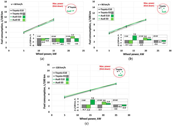
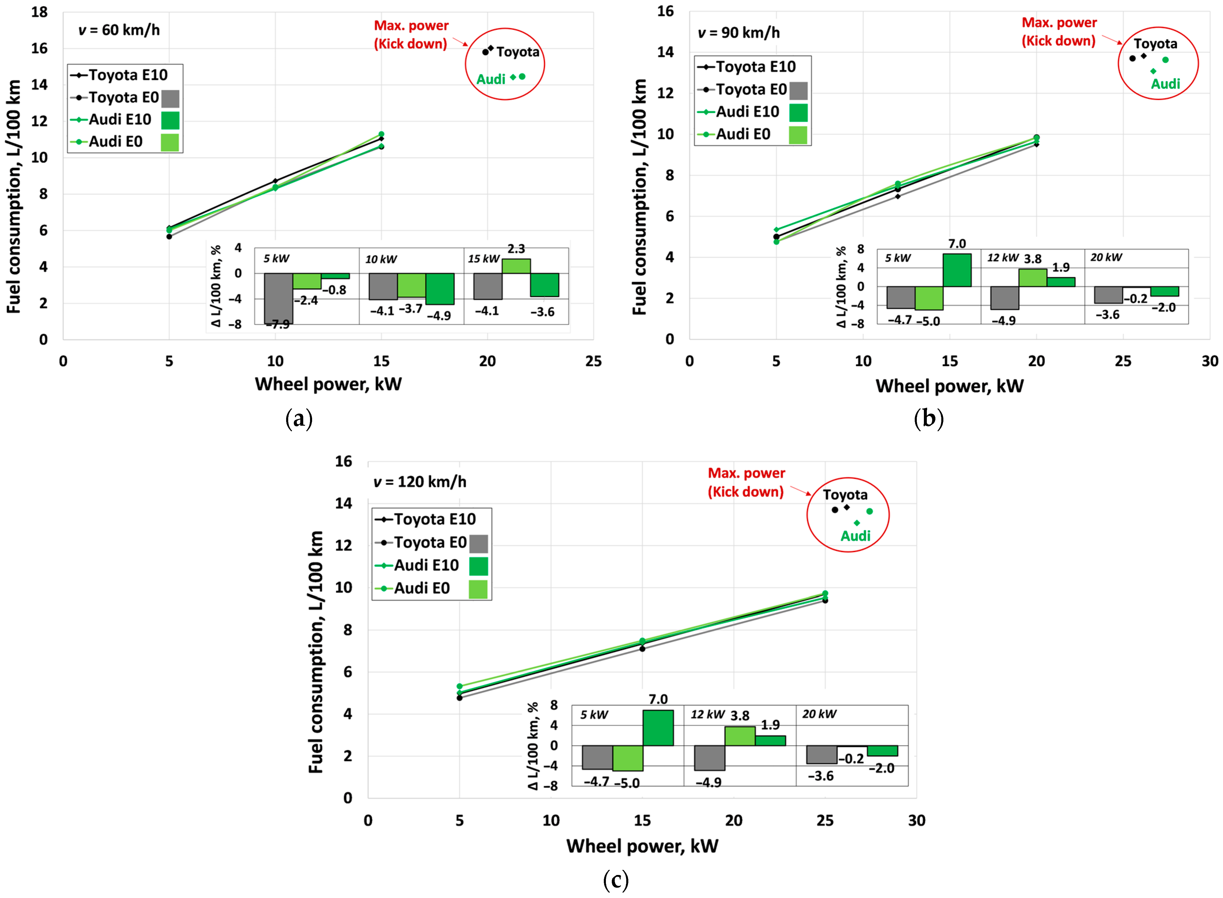
Comparison of fuel consumption for E10 and E0 at vehicle speeds of 60 (a), 90 (b), and 120 km/h (c) under different wheel power loads.
Figure 2.
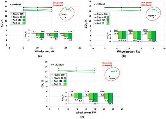
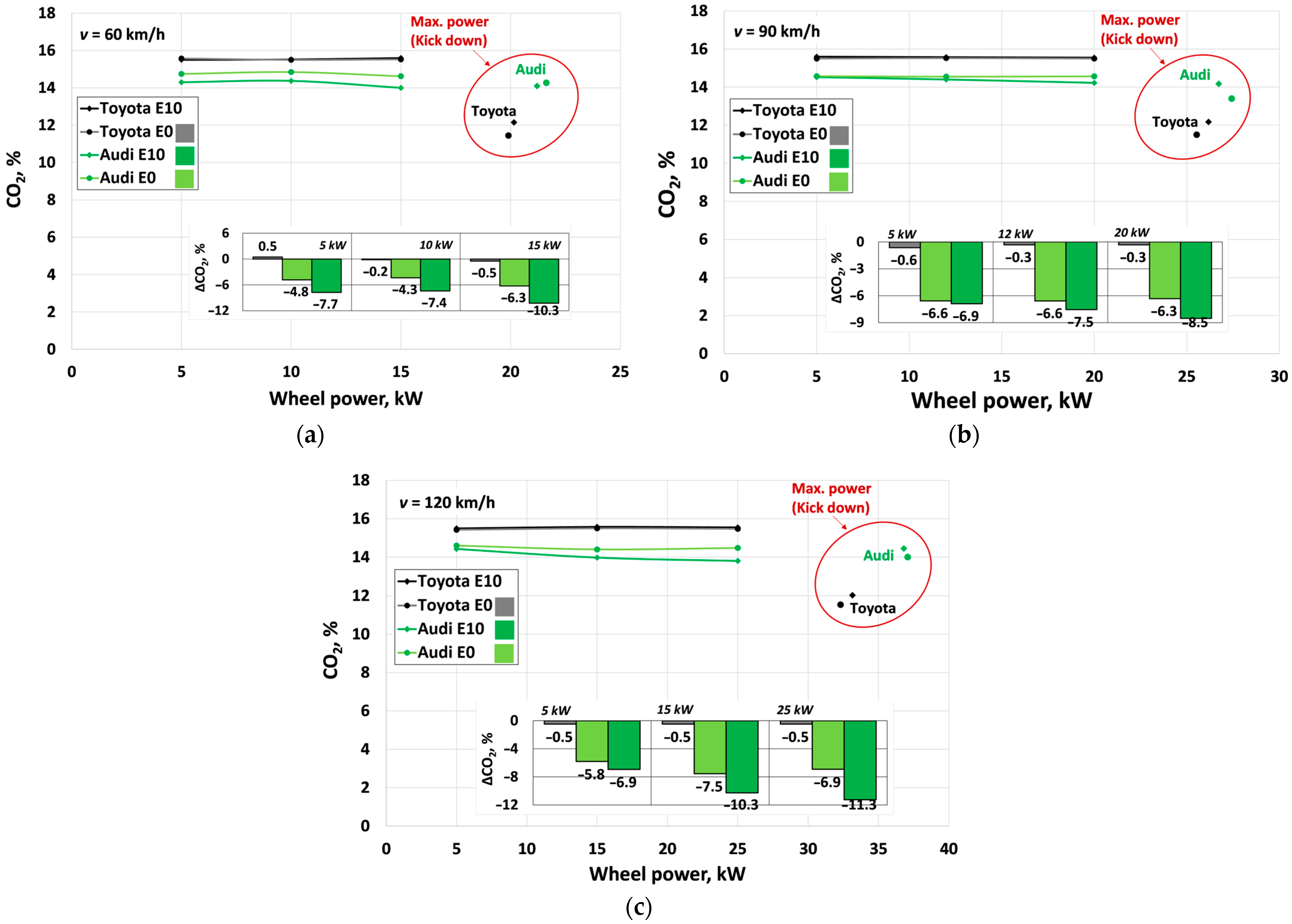
Comparison of Carbon dioxide (CO2) emission for E10 and E0 at vehicle speeds of 60 (a), 90 (b), and 120 km/h (c) under different wheel power loads.
Figure 3.
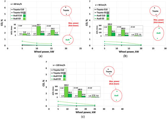
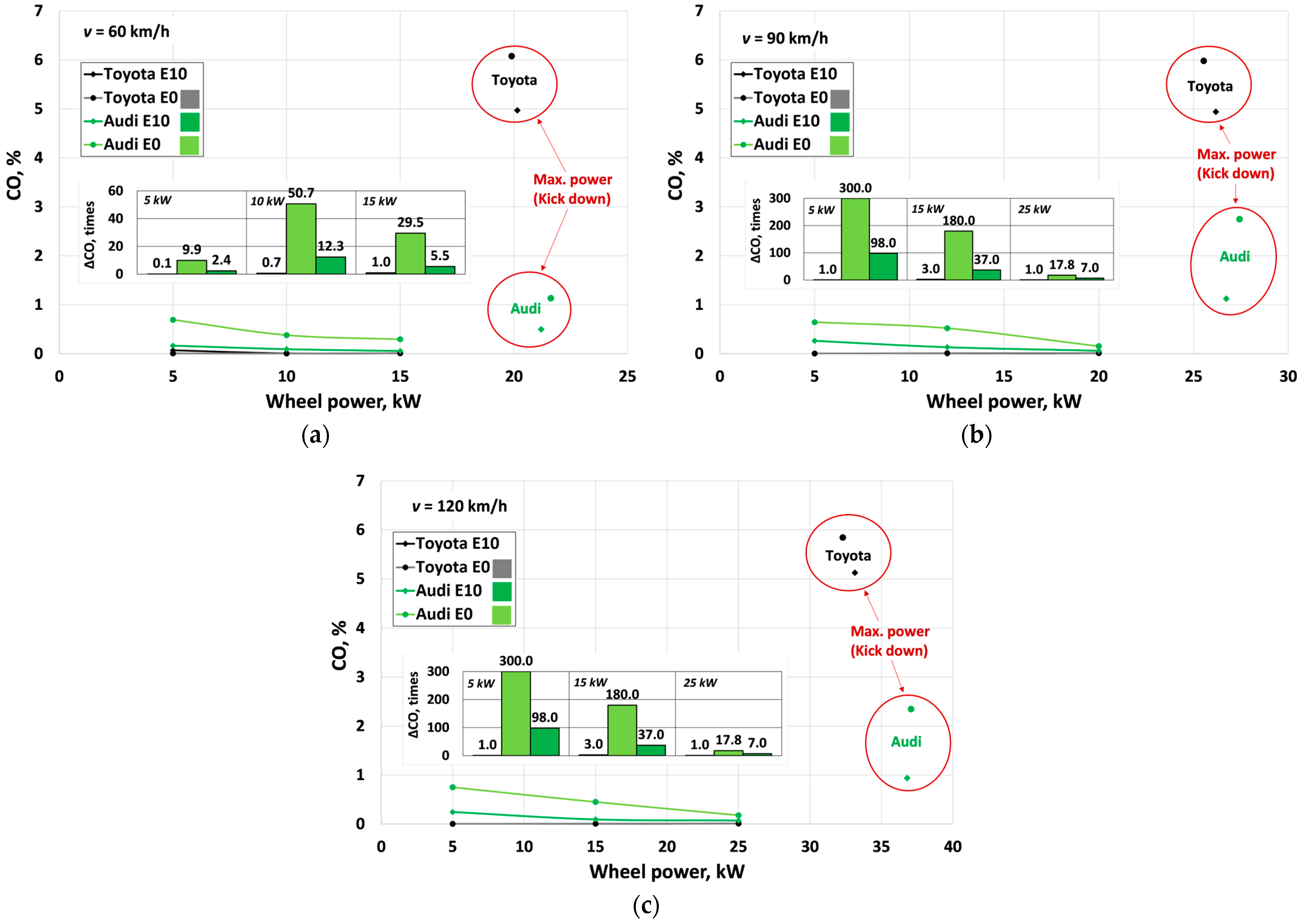
Comparison of Carbon monoxide (CO) emission for E10 and E0 at vehicle speeds of 60 (a), 90 (b), and 120 km/h (c) under different wheel power loads.
Figure 4.
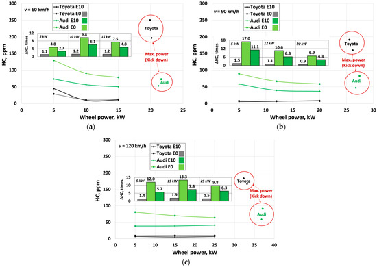
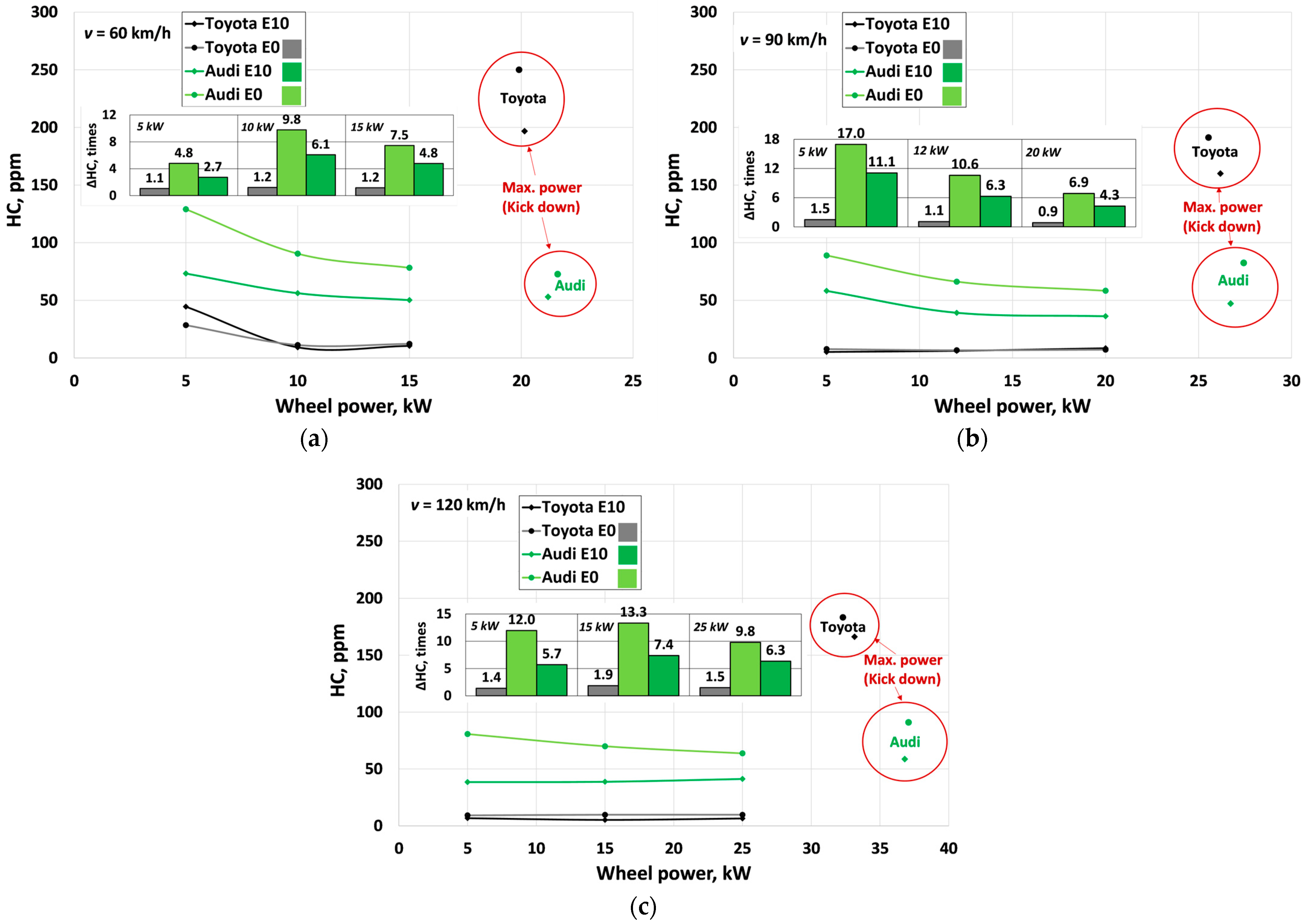
Comparison of Hydrocarbons (HC) emission for E10 and E0 at vehicle speeds of 60 (a), 90 (b), and 120 km/h (c) under different wheel power loads.
Figure 5.
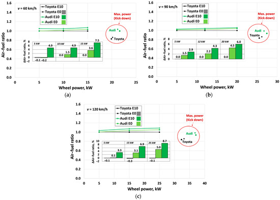
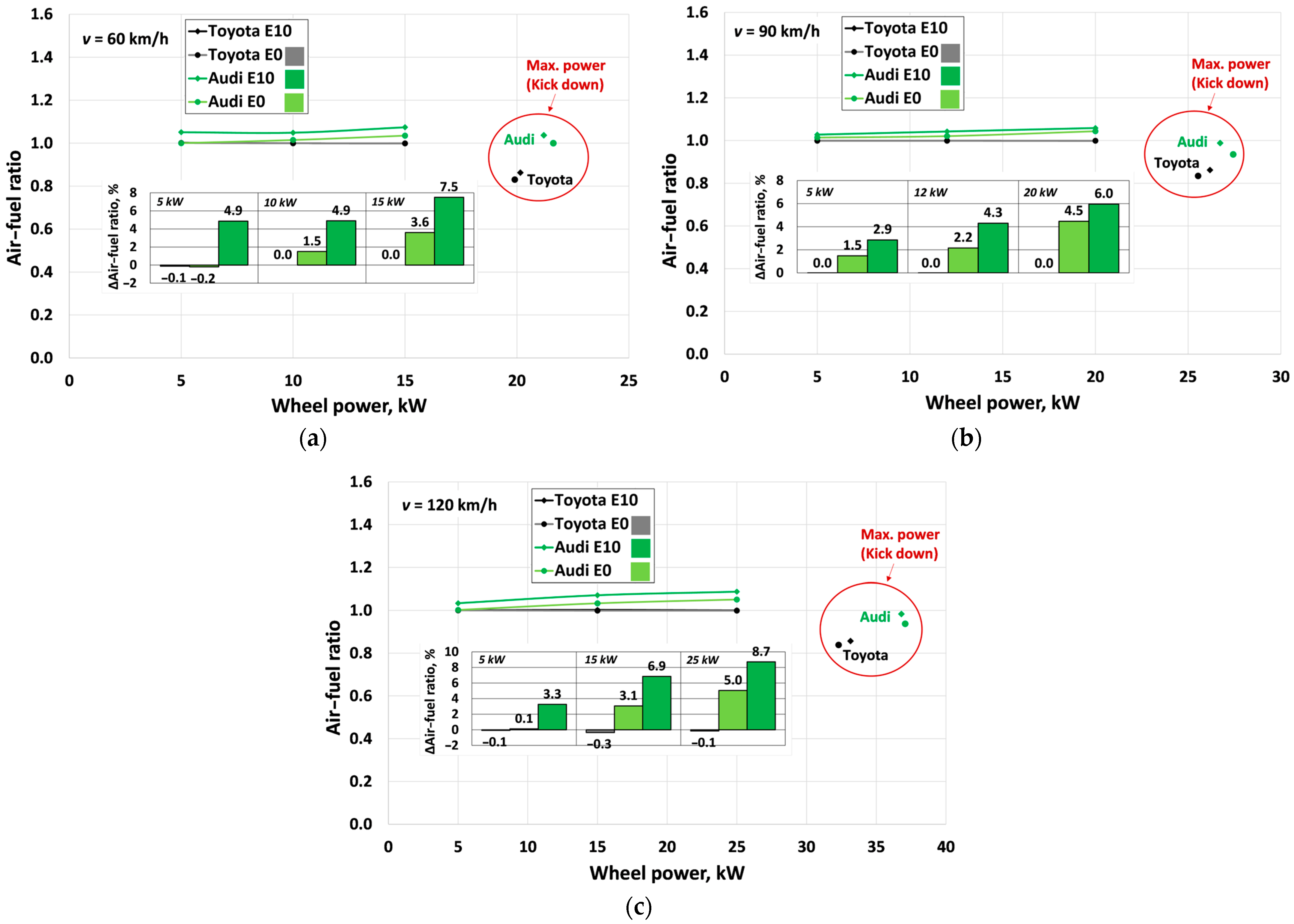
Comparison of Air–fuel ratio for E10 and E0 at vehicle speeds of 60 (a), 90 (b), and 120 km/h (c) under different wheel power loads.
Figure 6.
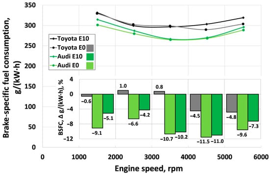
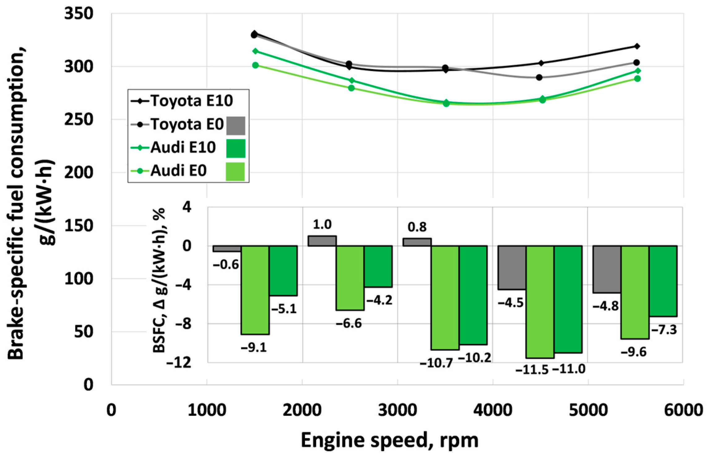
Brake-specific fuel consumption as a function of engine speed for E10 and E0 fuels during full-load engine acceleration tests.
To assess data dispersion and measurement repeatability, the spread of experimental results around the arithmetic mean was analysed using standard statistical indicators. The standard deviation (σ) was calculated for each measurement point to quantify variability. Confidence intervals were defined based on the ±σ criterion relative to the calculated mean value. In order to ensure a high level of experimental reliability, an acceptance threshold was established such that the relative deviation (±σ) could not exceed ±5% of the mean value for the evaluated parameter.
If the calculated dispersion exceeded this ±5% limit at any specific operating point, the corresponding experimental tests were repeated until the variability fell within the predefined tolerance range. This procedure ensured sufficient repeatability and minimised the influence of random measurement errors.
Although the graphical representation of standard deviation bands was omitted from Figure 1, Figure 2, Figure 3, Figure 4, Figure 5 and Figure 6 to maintain clarity and readability, the uncertainty assessment described above was systematically applied to all recorded energy and emission-related parameters throughout the entire study. Consequently, the presented results represent statistically validated mean values obtained under controlled and repeatable experimental conditions.
2.7. Test Boundary Conditions
To ensure reproducibility and transparency of the experimental framework, the boundary conditions, fuel characteristics, and data acquisition procedures applied in this study are summarised below.
All experiments were conducted on a chassis dynamometer under controlled laboratory conditions. Ambient temperature and atmospheric pressure were monitored during testing. Power-related parameters were corrected automatically by the dynamometer control system according to the applicable standard correction procedure implemented in the MAHA test bench software (MAHA LPS 2000). Emission measurements were performed using an AVL DiCom 4000 gas analyser. Since the study focuses on comparative analysis under identical laboratory conditions, all fuel tests (E0 and E10) were performed within the same day to minimize the influence of environmental variation.
Both vehicles were tested in the same transmission gear during steady-state operation to ensure consistent drivetrain efficiency and comparable wheel power levels. Prior to data acquisition, the engines were warmed up to stable operating temperatures. Coolant and lubricating oil temperatures were within normal operating ranges defined by the vehicle manufacturer. For the MPI vehicle, closed-loop λ control was confirmed to be active during part-load steady-state testing. The three-way catalytic converter was fully warmed up and operating within its effective temperature window before measurements were recorded.
In contrast, the carbureted vehicle was not equipped with exhaust aftertreatment. Therefore, the measured emissions represent raw engine-out values after dilution in the exhaust system.
For each vehicle speed and load condition, steady-state operation was established before data acquisition. Engine speed, wheel power, and air–fuel ratio were allowed to stabilize prior to recording. Sampling duration at each measurement point ranged from approximately 3 to 5 min, depending on parameter stability. Data recording was continued until fluctuations of the monitored variables remained within predefined repeatability limits.
Full-load (kickdown) measurements were performed separately from steady-state tests. These conditions represent enrichment-controlled operation (λ < 1) and were analysed independently from near-stoichiometric steady-state regimes.
3. Results and Discussion
3.1. Steady-State Part-Load Results
Fuel consumption is presented as distance specific volumetric values (L/100 km) at vehicle speeds of 60, 90, and 120 km/h (Figure 1). The connected data points from 5 kW up to 15 or 25 kW, depending on vehicle speed, represent steady part load operation, during which both engines were operated as close as possible to λ ≈ 1.0. The separate “Max. power” (kickdown) points correspond to full-throttle operation, during which the mixture was enriched (λ < 1) for both the MPI system and the carbureted engine. The same speed points and reference definition are used in subsequent figures. Operation of the Toyota equipped with MPI on E10 was selected as the reference case, and the diagrams illustrate the relative difference in fuel consumption (%) for the other configurations at the same wheel power.
Operation of the MPI system on pure gasoline (E0) resulted in lower fuel consumption compared to E10 by approximately 3–5% across most part-load points and by up to about 8% at the lowest wheel power. For example, the difference reaches −7.9% at 60 km/h and 5 kW and remained within approximately −3 to −5% at 90–120 km/h over the main part-load region. This trend is consistent with the lower volumetric energy content of E10, which has approximately 3.3% lower heating value per litre than E0. The Audi equipped with a carburetor (CARB) did not exhibit the same systematic deviation to the MPI operating on E10. Depending on vehicle speed and wheel power, CARB operation could be very close to MPI E10 or differ by several percent in either direction. At 120 km/h CARB on E0 ranges from approximately +0.3 to +7%, while CARB on E10 was closer to the MPI E10 reference, between −1.7 and +1%. Thus, the difference between MPI and CARB configurations depends strongly on the operating point, which is consistent with the distinct fuel metering principles (MPI vs. CARB) and their different sensitivity to engine speed and load.
Under maximum-load (kickdown) conditions, the combustible mixture in both vehicles is enriched to increase engine power and reduce the risk of knock (Figure 5). In the case of the Toyota (MPI), the mixture is enriched more substantially, reaching λ = 0.83–0.863, whereas in the Audi (CARB) configuration enrichment is limited to λ = 0.935–1.037. This difference directly influences fuel consumption behaviour. At vehicle speeds of 60 and 90 km/h, the effect is less pronounced; however, when the speed is increased to 120 km/h under full-throttle operation, a sharp increase in fuel consumption is observed (Figure 1).
The comparison of emissions between the MPI and CARB configurations must be interpreted with caution because the MPI vehicle is equipped with a three-way catalytic converter (TWC), whereas the CARB vehicle has no exhaust aftertreatment. Consequently, the results represent complete vehicle systems, and direct comparison of absolute tailpipe emission levels between MPI and CARB is limited. At part load near λ ≈ 1.0, MPI tailpipe emissions are strongly influenced by TWC conversion efficiency. Therefore, the absolute differences in CO and HC emissions between MPI and CARB mainly reflect the combined effect of engine combustion characteristics and the presence or absence of aftertreatment. In the CARB engine, a portion of the fuel carbon may leave the exhaust as CO or HC rather than being fully oxidised to CO2, resulting in lower measured CO2 concentrations. CO2 is reported as exhaust concentration (vol. %) (Figure 2) and is strongly affected by excess air dilution. For the MPI configuration, CO2 concentrations at part load are relatively stable, and the difference between E0 and E10 is small (approximately 0 to –0.6% relative to MPI E10). In contrast, the CARB configurations exhibit lower CO2 concentrations, with the deviation increasing as load rises. At 60 km/h, CARB E10 ranges from –7.4 to –10.3% relative to MPI E10 over 10–15 kW, while CARB E0 ranges from −4.8 to −6.3%. At 90 km/h, CARB E10 ranges from −6.9 to −8.5% and CARB E0 from −6.3 to −6.6%. At 120 km/h, CARB E10 ranges from −6.9 to −11.3% and CARB E0 from −5.8 to −7.5%. Thus, the observed differences in CO2 between MPI and CARB configurations primarily reflect mixture-related dilution effects (λ and O2 concentration) rather than differences in carbon conversion efficiency alone.
Under maximum-load (kickdown) operation, a decrease in the measured CO2 concentration in the exhaust gas is observed. This trend is expected because, as the excess-air ratio decreases (λ < 1), the combustion process becomes oxygen-deficient due to mixture enrichment. Under such conditions, a larger fraction of the fuel carbon is not fully oxidised to CO2 and instead appears as products of incomplete combustion, primarily carbon monoxide (CO) and unburned hydrocarbons (HC).
CO is presented as exhaust concentration (vol. %) (Figure 3). In the MPI configuration, CO levels at part load are close to zero; therefore, the relative differences are expressed as multiples (×) of the MPI E10 reference values. MPI operation on E0 remains close to MPI E10, ranging from approximately 0.1 to 4×, depending on wheel power.
In contrast, the CARB configuration exhibits substantially higher CO concentrations at part load, particularly when operating on E0. Relative to MPI E10, CO levels for CARB on E0 reach 9.9–50.7× at 60 km/h, 15.3–257× at 90 km/h, and 17.8–300× at 120 km/h. When operating onE10, CARB CO levels are lower, ranging from 2.4 to 12.3×, 6.0 to 105×, and 7.0 to 98× at 60, 90, and 120 km/h, respectively.
Under maximum-load (kickdown) conditions, both engines exhibit increased CO concentrations, consistent with mixture enrichment. In the MPI configurations, CO rises from approximately 0.01% at part load to 5.8 to 6.1% on E0 and 4.9 to 5.1% on E10. The CARB configurations show lower CO concentrations under kickdown conditions than MPI, as it operate with a less rich at full throttle (MPI λ ≈ 0.83–0.86, CARB λ ≈ 0.94–0.99).
The influence of fuel composition remains evident: when operating on E10, CARB CO concentrations decrease by approximately 56–60%, from 1.14 to 2.75% (E0) to 0.50 to 1.12% (E10), depending on vehicle speed.
The enrichment effect is most clearly reflected in the measured CO concentrations. This behaviour is particularly pronounced for the Toyota equipped with the MPI system, where the air–fuel mixture is enriched to reach the maximum attainable engine power. Under these oxygen-deficient conditions (λ < 1), complete oxidation of carbon to CO2 is limited, and a larger fraction of carbon is converted to CO, resulting in a substantial increase in CO emissions. At this point, the TWC is also less effective in reducing CO because high CO conversion efficiency requires sufficient oxygen availability in the exhaust gas. During strongly enriched operation, the lack of oxygen limits oxidation reactions in the catalyst, and therefore the tailpipe CO level remains high despite the presence of aftertreatment.
HC emissions are presented as concentration (ppm) (Figure 4). The elative differences in HC are expressed as multiples (×) of the MPI E10 reference values. In the MPI configuration, HC emissions remain low, and MPI operation on E0 is close to MPI E10, typically ranging from 0.9 to 1.9×. In contrast, the CARB configuration exhibits substantially higher HC concentrations at part load, particularly when operating on E0. Relative to MPI E10, CARB on E0 reaches 4.8–9.8× at 60 km/h, 6.9–17× at 90 km/h, and 9.8–13.3× at 120 km/h. When operating on E10, HC levels in the CARB configuration are lower, ranging from 2.7 to 6.1× at 60 km/h, 4.3 to 11.1× at 90 km/h, and 5.7 to 7.4× at 120 km/h. These results indicate that E10 reduces HC emissions in the CARB configuration by approximately 1.5–2.5× compared to CARB operation on E0 at the same operating points. This behaviour is consistent with the leaner mixture formation observed with E10 in the carbureted system and the absence of catalytic aftertreatment.
Under maximum-load (kickdown) conditions, HC emissions increases, particularly in the MPI configuration (approximately 160–250 ppm), whereas CARB values remain lower (50–90 ppm). This difference corresponds to the richer full-throttle operation of the MPI system (λ < 1), while the CARB configuration remains closer to stoichiometric conditions (λ = 1) at maximum load.
The air–fuel ratio (λ) is presented in Figure 5. The MPI configuration operates close to stoichiometric conditions at part load for both fuels. MPI operation on E0 is nearly identical to MPI E10, with deviations ranging from −0.1 to 0.0% at 60–90 km/h, and from −0.1 to −0.3% at 120 km/h. This behaviour is consistent with closed-loop λ control, which maintains λ ≈ 1.0 under part-load conditions.
In contrast, the CARB configuration operates under leaner conditions (λ > 1) and becomes even leaner when fueled with E10 compared to E0. Relative to MPI E10, at 60 km/h CARB E0 varies from −0.2% at 5 kW to +3.6% at 15 kW, while CARB E10 reaches +4.9% at 5–10 kW and +7.5% at 15 kW. At 90 km/h, CARB E0 shows deviations of +1.5%, +2.2%, and +4.5% at 5, 12, 20 kW, respectively, whereas CARB E10 reaches +2.9%, +4.3%, +6.0%. At 120 km/h, CARB E0 shows +0.1%, +3.1%, +5.0% for 5, 15, 25 kW and CARB E10 is +3.3%, +6.9%, +8.7%.
This behaviour is consistent with fixed carburetor jetting. Since E10 has a lower stoichiometric air–fuel ratio than E0, the same jet configuration results in a higher excess-air ratio (λ), and this effect becomes more pronounced with increasing load.
3.2. Full-Throttle Results
Brake-specific fuel consumption (BSFC) is presented in g/(kWh) as a function of engine speed (Figure 6). In this part of the study, the measurements were performed using a full-throttle engine speed sweep. The test was conducted at discrete engine-speed points with a step of 1000 rpm over the range from 1500 to 5500 rpm. This procedure was selected because the chassis dynamometer provides an automated control mode that precisely regulates the predefined operating points and maintains each point for a user-defined duration, ensuring stable conditions for data acquisition. Importantly, the dynamometer accounts for drivetrain losses across the entire operating range and automatically calculates brake-specific fuel consumption (BSFC) based on engine brake power, rather than wheel (traction) power, thereby improving the comparability of results across different operating points.
For both engine configurations, BSFC is higher at low and high engine speeds and reaches its minimum in the mid-speed range. For the MPI system, BSFC is approximately 330 g/(kWh) at ~1500 rpm, decreases to about 295–300 g/(kWh) in the mid-range (~2500–4500 rpm), and increases again to approximately 320 g/(kWh) at ~5600 rpm. For the CARB configuration, BSFC is lower across the entire speed range: approximately 300–315 g/(kWh) at ~1500 rpm, 265–270 g/(kWh) around ~3500–4500 rpm, and 290–300 g/(kWh) at ~5600 rpm. For both engine setups, operation on E0 results in slightly lower BSFC than E10 at most speed points. The difference is relatively small in the mid-speed range but becomes more pronounced at the lowest and highest engines speeds.
Since E10 contains oxygen, its stoichiometric air/fuel ratio is lower than of E0. In the MPI configuration, this additional oxygen does not significantly affect λ under part-load conditions, because the closed loop control system compensates by adjusting fuel delivery to maintain λ ≈ 1.0. Consequently, the primary influence on BSFC remains the lower heating value (LHV) of E10, which leads to a slight increase in specific fuel consumption.
In contrast, the CARB system employs fixed jetting; therefore, changing to E10 shifts λ toward a leaner mixture. This affects the thermodynamic efficiency of energy conversion at different speed-load combinations, which explains why the BSFC difference between E10 and E0 is not constant across the engine speed range.
4. Conclusions
Experimental chassis dynamometer tests were performed using two spark-ignition engine configurations–multi-point fuel injection (MPI) and carbureted (CARB)—with E0 and E10 fuels. Measurements were conducted at steady-state part load conditions (5–15/25 kW, λ ≈ 1.0) at vehicle speeds of 60, 90, and 120 km/h, as well as under separate full-throttle “maximum power” (kickdown) conditions with mixture enrichment (λ < 1).
1. For the MPI-equipped vehicle, the use of E0 resulted in consistently lower volumetric fuel consumption and brake-specific fuel consumption compared to E10. The observed reduction (approximately 3–5% at most part-load operating points and up to about 8% at low loads) corresponds well to the lower volumetric heating value of E10, confirming that closed-loop λ control effectively compensates for the oxygen content of ethanol but cannot offset its lower energy density. In the carbureted engine, the differences in fuel consumption between E0 and E10 were less systematic and strongly dependent on engine speed and load. Due to fixed jetting, the use of E10 led to a leaner air–fuel mixture, which in some operating regions reduced brake-specific fuel consumption, while in others it increased it. This highlights the higher sensitivity of carbureted systems to changes in fuel composition.
2. Carbon dioxide (CO2) concentrations in the exhaust gas were relatively stable and similar for both fuels in the MPI engine, reflecting near-stoichiometric combustion. In contrast, the carbureted engine exhibited significantly lower CO2 concentrations, primarily due to leaner operation and increased dilution by excess air, rather than a direct reduction in carbon conversion efficiency.
3. Carbon monoxide (CO) and unburned hydrocarbon (HC) emissions were strongly influenced by both the fuel supply system and the presence of exhaust aftertreatment. The MPI-equipped vehicle exhibited very low CO and HC emissions at part load for both E0 and E10 fuels, which can be primarily attributed to stoichiometric combustion control combined with the use of a three-way catalytic (TWC) converter. In contrast, the carbureted engine, which was not equipped with a catalytic converter, showed substantially higher CO and HC emissions, particularly when operating on E0. The use of E10 significantly reduced CO and HC emissions in the carbureted engine due to the oxygen content of ethanol and the resulting leaner mixture formation.
4. Overall, the results indicate that engines equipped with electronic fuel injection systems are more robust to sudden changes in fuel composition between E10 and E0, maintaining stable air–fuel ratio control and predictable performance. In contrast, carbureted engines are more sensitive to such transitions, exhibiting pronounced variations in mixture formation, fuel consumption, and exhaust emissions. From a practical standpoint, a temporary shift from E10 to E0—such as one that may occur during fuel supply disruptions—is therefore expected to have a limited impact on modern MPI-equipped vehicles, while potentially causing significant changes in emissions and operating characteristics of older carbureted engines and small generator units.
Author Contributions
Conceptualisation, G.M. and S.P.; methodology, G.M. and S.P.; software, S.P. and S.N.; validation, G.M., A.R., and S.N.; formal analysis, A.R.; investigation, S.P. and S.N.; resources, S.P.; data curation, A.R. and S.N.; writing—original draft preparation, G.M. and S.P.; writing—review and editing, A.R. and S.N.; visualisation, S.P. and S.N.; supervision, S.P.; project administration, S.P. All authors have read and agreed to the published version of the manuscript.
Funding
This research received no external funding.
Institutional Review Board Statement
Not applicable.
Informed Consent Statement
Not applicable.
Data Availability Statement
The original contributions presented in this study are included in the article. Further inquiries can be directed to the corresponding author.
Conflicts of Interest
The authors declare no conflicts of interest.
Abbreviations
The following abbreviations are used in this manuscript:
| BSFC | Brake-specific fuel consumption |
| CARB | Carburetor |
| CO | Carbon monoxide |
| CO2 | Carbon dioxide |
| E0 | Pure gasoline |
| E10 | Gasoline blended with 10% ethanol |
| FID | Flame ionisation |
| HC | Hydrocarbons |
| LHV | Lower heating value |
| MPI | Multi-point injection |
| NDIR | Non-Dispersive Infrared |
| O2 | Oxygen |
References
- Miskat, M.I.; Ahmed, A.; Chowdhury, H.; Chowdhury, T.; Chowdhury, P.; Sait, S.M.; Park, Y.-K. Assessing the Theoretical Prospects of Bioethanol Production as a Biofuel from Agricultural Residues in Bangladesh: A Review. Sustainability 2020, 12, 8583. [Google Scholar] [CrossRef] [Scilit]
- Zeb, K.; Ali, S.M.; Khan, B.; Mehmood, C.A.; Tareen, N.; Din, W.; Farid, U.; Haider, A. A Survey on Waste Heat Recovery: Electric Power Generation and Potential Prospects within Pakistan. Renew. Sustain. Energy Rev. 2017, 75, 1142–1155. [Google Scholar] [CrossRef] [Scilit]
- Solaymani, S.; Botero, J. Reducing Carbon Emissions from Transport Sector: Experience and Policy Design Considerations. Sustainability 2025, 17, 3762. [Google Scholar] [CrossRef] [Scilit]
- National Research Council. Advancing the Science of Climate Change; National Academies Press: Washington, DC, USA, 2010. [Google Scholar]
- National Research Council. Transitions to Alternative Vehicles and Fuels; National Academies Press: Washington, DC, USA, 2013. [Google Scholar]
- Munsin, R.; Laoonual, Y.; Jugjai, S.; Imai, Y. An Experimental Study on Performance and Emissions of a Small SI Engine Generator Set Fuelled by Hydrous Ethanol with High Water Contents up to 40%. Fuel 2013, 106, 586–592. [Google Scholar] [CrossRef] [Scilit]
- Mužíková, Z.; Pospíšil, M.; Šebor, G. Volatility and Phase Stability of Petrol Blends with Ethanol. Fuel 2009, 88, 1351–1356. [Google Scholar] [CrossRef] [Scilit]
- Misron, N.; Rizuan, S.; Vaithilingam, A.; Mailah, N.F.; Tsuyoshi, H.; Hiroaki, Y.; Yoshihito, S. Performance Improvement of a Portable Electric Generator Using an Optimized Bio-Fuel Ratio in a Single Cylinder Two-Stroke Engine. Energies 2011, 4, 1937–1949. [Google Scholar] [CrossRef] [Scilit]
- Shi, X.; Qian, W.; Wang, Q.; Luo, H.; Kang, Y.; Ni, J. Effect of Water Content of Hydrous Ethanol on Chemical Kinetic Characteristics Based on the New Developed Reduced Ethanol-Toluene Reference Fuels Mechanism. Fuel 2021, 303, 121201. [Google Scholar] [CrossRef] [Scilit]
- Iodice, P.; Cardone, M. Ethanol/Gasoline Blends as Alternative Fuel in Last Generation Spark-Ignition Engines: A Review on CO and HC Engine Out Emissions. Energies 2021, 14, 4034. [Google Scholar] [CrossRef] [Scilit]
- Yao, Y.-C.; Tsai, J.-H.; Wang, I.-T. Emissions of Gaseous Pollutant from Motorcycle Powered by Ethanol–Gasoline Blend. Appl. Energy 2013, 102, 93–100. [Google Scholar] [CrossRef] [Scilit]
- Tibaquirá, J.; Huertas, J.; Ospina, S.; Quirama, L.; Niño, J. The Effect of Using Ethanol-Gasoline Blends on the Mechanical, Energy and Environmental Performance of In-Use Vehicles. Energies 2018, 11, 221. [Google Scholar] [CrossRef] [Scilit]
- Jia, L.-W.; Shen, M.-Q.; Wang, J.; Lin, M.-Q. Influence of Ethanol–Gasoline Blended Fuel on Emission Characteristics from a Four-Stroke Motorcycle Engine. J. Hazard. Mater. 2005, 123, 29–34. [Google Scholar] [CrossRef] [Scilit]
- Karavalakis, G.; Durbin, T.D.; Shrivastava, M.; Zheng, Z.; Villela, M.; Jung, H. Impacts of Ethanol Fuel Level on Emissions of Regulated and Unregulated Pollutants from a Fleet of Gasoline Light-Duty Vehicles. Fuel 2012, 93, 549–558. [Google Scholar] [CrossRef] [Scilit]
- Wongsurakul, P.; Termtanun, M.; Kiatkittipong, W.; Lim, J.W.; Kiatkittipong, K.; Pavasant, P.; Kumakiri, I.; Assabumrungrat, S. Comprehensive Review on Potential Contamination in Fuel Ethanol Production with Proposed Specific Guideline Criteria. Energies 2022, 15, 2986. [Google Scholar] [CrossRef] [Scilit]
- Yoo, Y.H.; Park, I.J.; Kim, J.G.; Kwak, D.H.; Ji, W.S. Corrosion Characteristics of Aluminum Alloy in Bio-Ethanol Blended Gasoline Fuel: Part 1. The Corrosion Properties of Aluminum Alloy in High Temperature Fuels. Fuel 2011, 90, 1208–1214. [Google Scholar] [CrossRef] [Scilit]
- Amine, M.; Awad, E.N.; Ibrahim, V.; Barakat, Y. Effect of Ethyl Acetate Addition on Phase Stability, Octane Number and Volatility Criteria of Ethanol-Gasoline Blends. Egypt. J. Pet. 2018, 27, 567–572. [Google Scholar] [CrossRef] [Scilit]
- Matějovský, L.; Macák, J.; Pospíšil, M.; Baroš, P.; Staš, M.; Krausová, A. Study of Corrosion of Metallic Materials in Ethanol–Gasoline Blends: Application of Electrochemical Methods. Energy Fuels 2017, 31, 10880–10889. [Google Scholar] [CrossRef] [Scilit]
- Kumar, T.S.; Ashok, B. Corrosion Behaviour Analysis of SI Engine Components for Ethanol-Gasoline Blends in Flex Fuel Vehicular Application. Fuel Process. Technol. 2023, 240, 107574. [Google Scholar] [CrossRef] [Scilit]
- Baena, L.M.; Vásquez, F.A.; Calderón, J.A. Corrosion Assessment of Metals in Bioethanol-Gasoline Blends Using Electrochemical Impedance Spectroscopy. Heliyon 2021, 7, e07585. [Google Scholar] [CrossRef] [Scilit]
- Brito-Franco, A.; Uruchurtu, J.; Rosales-Cadena, I.; Lopez-Sesenes, R.; Serna-Barquera, S.A.; Hernandez-Perez, J.A.; Rocabruno-Valdes, C.; Gonzalez-Rodriguez, J.G. Corrosion Behavior of Al in Ethanol–Gasoline Blends. Energies 2020, 13, 5544. [Google Scholar] [CrossRef] [Scilit]
- Turanov, A.; Khitrin, A.K. Ethanol Clusters in Gasoline-Ethanol Blends. Ind. Eng. Chem. Res. 2016, 55, 9952–9955. [Google Scholar] [CrossRef] [Scilit]
- Kyriakides, A.; Dimas, V.; Lymperopoulou, E.; Karonis, D.; Lois, E. Evaluation of Gasoline–Ethanol–Water Ternary Mixtures Used as a Fuel for an Otto Engine. Fuel 2013, 108, 208–215. [Google Scholar] [CrossRef] [Scilit]
- Baena, L.M.; Gómez, M.; Calderón, J.A. Aggressiveness of a 20% Bioethanol–80% Gasoline Mixture on Autoparts: I Behavior of Metallic Materials and Evaluation of Their Electrochemical Properties. Fuel 2012, 95, 320–328. [Google Scholar] [CrossRef] [Scilit]
- Warguła, Ł.; Wieczorek, B.; Gierz, Ł.; Karwat, B. Critical Concerns Regarding the Transition from E5 to E10 Gasoline in the European Union, Particularly in Poland in 2024—A Theoretical and Experimental Analysis of the Problem of Controlling the Air–Fuel Mixture Composition (AFR) and the λ Coefficient. Energies 2025, 18, 852. [Google Scholar] [CrossRef] [Scilit]
- Santos, E.D.S.; Silva, W.D.O.; Fontana, M.E.; Marques, P.C.; Pedro, H.C.; Mota, R.D.O.; Nepomuceno, V. Circular Strategic Options for Ethanol Supply Chain Resilience Under Uncertainties Using a Composition of Probabilities Group Decision Model. Logistics 2025, 9, 71. [Google Scholar] [CrossRef] [Scilit]
- Gajewski, M.; Wyrąbkiewicz, S.; Kaszkowiak, J. Effects of Ethanol–Gasoline Blends on the Performance and Emissions of a Vehicle Spark-Ignition Engine. Energies 2025, 18, 3466. [Google Scholar] [CrossRef] [Scilit]
- Chen, W.; Bock, N.; Northrop, W.; Kittelson, D. Influence of Combustion Strategy and Fuel Ethanol Content on Effective Density, Concentration, and Size of Particles Emitted by a Lean Burn Gasoline Direct Injection Engine. Emiss. Control Sci. Technol. 2025, 11, 29. [Google Scholar] [CrossRef] [Scilit]
- DIN 70200:2012-06; Technical Product Documentation—System of Documentation—General Principles. Beuth Verlag (DIN Media): Berlin, Germany, 2012.

Disclaimer/Publisher’s Note: The statements, opinions and data contained in all publications are solely those of the individual author(s) and contributor(s) and not of MDPI and/or the editor(s). MDPI and/or the editor(s) disclaim responsibility for any injury to people or property resulting from any ideas, methods, instructions or products referred to in the content. |
© 2026 by the authors. Licensee MDPI, Basel, Switzerland. This article is an open access article distributed under the terms and conditions of the Creative Commons Attribution (CC BY) license.