


Abstract
This paper presents a minimally intrusive experimental methodology for identifying and modeling power losses in the electric powertrain of a battery electric vehicle, including the inverter, electric motor and speed reducer. Measurements are performed on a roller test bench equipped with an eddy current brake, using two complementary approaches to determine the mechanical power at the wheel: (i) a direct measurement based on an onboard rotary torque sensor integrated into a driveshaft; (ii) an indirect estimation derived from brake power measurements corrected for bench losses and tire longitudinal slip. The two approaches are systematically compared in order to quantify the accuracy loss associated with brake-based measurements and to identify the operating conditions under which they can reliably substitute direct torque measurements. The experimental results show that brake-based estimations provide acceptable accuracy at moderate–high torque levels, while significant deviations occur at low torque. Based on the experimental dataset, an overall power loss model is identified using a polynomial function of motor torque and speed. Two fitting strategies are investigated: an unconstrained least-squares approach, allowing all coefficients to vary freely, and a constrained formulation enforcing physically admissible (non-negative) loss terms; while the unconstrained method slightly improves the numerical fit, it may lead to non-physical coefficients and invalid efficiency predictions. In contrast, the constrained approach preserves physical interpretability and ensures consistent loss and efficiency maps. Finally, a step-by-step practical guide is provided to facilitate the implementation of the proposed methodology for powertrain loss identification on electric vehicles without extensive mechanical disassembly.
1. Introduction
The transition of the automotive industry to fully electric vehicles (EVs) is a key component in global efforts to combat climate change. In recent years, sales have seen a significant and steady increase, reaching 20 million EVs sold in 2025, accounting for one fourth cars sold worldwide [1]. This trend is expected to continue and even accelerate in the coming years [2]. As a result, numerous vehicle prototypes are being developed, and those already in production will require rigorous maintenance tracking to ensure long-term performance and reliability.
For these studies to be carried out, the staff in charge of EV energy performance must have access to the most efficient quantification method possible, which typically involve the use of efficiency or loss data maps [3,4,5].
The first approach for generating data maps relies on physical modeling of the system. Losses in AC electric machines can be modeled using the d-q axis method (Park transformation) [6,7,8]. Losses in the inverter, arising from conduction and/or switching phenomena, can also be modeled using approaches of varying complexity, ranging from simplified formulations [6] to more detailed models [7,8]. Finally, losses in the transmission—including gearing losses, sealing losses, and bearing losses—can likewise be modeled by accounting for the effects of load and rotational speed [9]. These approaches generally rely on manufacturer data, complemented by experimental measurements, which are at least used for model validation. In this case, the data maps are directly generated by the models and do not require additional data-fitting technique.
A second approach relies exclusively on experimental data. In this case, the generation of data maps requires the application of data-fitting technique, along with validation methods to mitigate the risks of under-fitting and over-fitting. This latter approach can be further divided into two sub-categories.
The first consists of isolating the components to be characterized on a dedicated test bench, specifically designed for this purpose. This methodology requires dismantling the vehicle under study. The measurement techniques employed are generally conventional and, as a result, are often only briefly described in the literature. Examples of such approaches can be found in [6,10].
The second sub-approach aims to avoid dismantling the vehicle by performing measurements on a complete one, either under real driving conditions [11] or on a roller test bench [7,12]. In this case, in addition to the previously mentioned losses, tire power losses, mainly due to longitudinal slip, must be considered. When these losses are not intended to be included in the analysis, it may be relevant to directly measure the torque—and thus the power—transmitted upstream of the tire, by integrating a torque measurement device on the driveshaft. Such instrumentation can be implemented using various techniques [13] and represents an attractive compromise between measurement accuracy, vehicle intrusiveness, and test system development time. The authors of [14] describe such an approach applied to the measurement of transient torque in a hybrid electric vehicle.
However, to the authors’ knowledge, no publication has reported power loss measurements using an onboard torque sensor on a battery electric vehicle. The primary objective of this paper is to address this gap. The second objective is to present and detail polynomial analytical model fitting and validation techniques based on a physics-based approach, an aspect that is rarely addressed in the existing scientific literature. Finally, the third objective is to assess whether the addition of an on board torque sensor is strictly necessary, or whether power measurements performed downstream of the tire, combined with a tire slip loss model, can provide a reliable estimation of the power losses upstream of the tire.
Consequently, the experimental measurements will be conducted on a roller test bench, as it offers a practical and economical option commonly used in vehicle testing. The experimental vehicle underwent two minor modifications: the electrical circuit at the battery output was opened to insert a shunt for current measurement, and one of the final drive shafts was modified to incorporate a commercial ‘ready to use’ rotary torque sensor.
The paper is organized as follows: First, the considered power loss are presented together with the associated notation. The materials and methods are then described, including the experimental vehicle, the rotary torque meter, the roller test bench and the procedure used to calibrate mechanical friction losses in the latter. The issue of the equivalent mass of the vehicle, rotating components, and rollers is subsequently discussed. Finally, the theoretical framework for quantifying longitudinal slip and its compensation in the measurements is introduced and analyzed. Next, a loss modeling approach based on a two-variable polynomial function—torque and motor speed—will be proposed and discussed in detail, with the aim of considering only the dominant first-order physical effects.
The loss model coefficients will be identified using the least-squares method applied to both complete measurement datasets (torque meter and brake-based measurements). The method is briefly reviewed, and the risks of underfitting and overfitting are assessed using a cross-validation procedure.
The measurements and maps obtained from both measurement methods will be compared to assess how complementary they can be and to quantify the loss of accuracy associated with using the brake-based measurement method.
Finally, a step-by-step summary of the method will be provided to guide the reader through its implementation.
2. Power Losses of Electric Vehicle
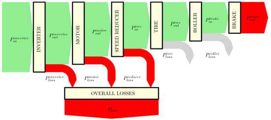
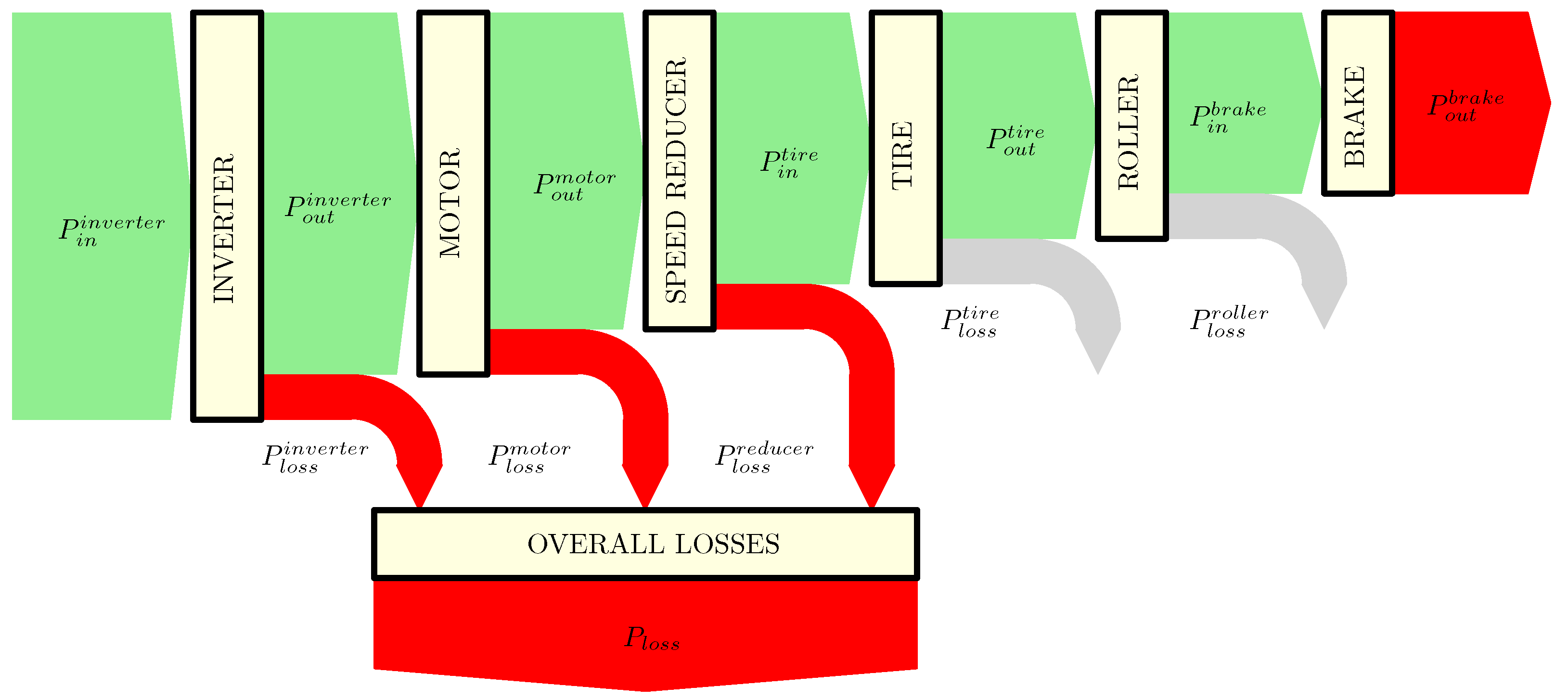
Figure 1 gives a Sankey diagram of the considered power losses for this study.
Figure 1.
SANKEY Diagram of the power losses for an electric vehicle.
Firstly, it should be noted that losses in the battery pack are beyond the scope of this paper and are not considered. Consequently, the input power is the electrical power supplied to the inverter by the battery pack, denoted as . The output power is the mechanical power delivered by the transmission shafts to the driven wheels, denoted as .
The overall power loss of the vehicle transmission, denoted as is the sum of power losses in inverter, electric motor and speed reducer, respectively, denoted as , and .
The measurement of electrical power has been performed by current and voltage measurements or using the CAN messaging from the Battery Management System, as discussed later in this paper.
The measurement of has been performed with two different approach. First method, which gives the best accuracy, uses both an embedded rotary torque meter (quantity ) and an angular speed measurement (quantity ) on the transmission shaft. By assuming that the power is the same at both driven wheel, it can be written as
The second method, in a case where no torque meter is used, estimates the tire power input from power measurement at the eddy current brake of the roller test bench, denoted as . In this case, two additional losses must be accounted for: tire longitudinal slip loss and roll test bench loss, respectively, denoted as and . The total friction losses in the test bench (including rollers and brake losses) will be determined through a calibration process, while the tire losses will be determined from measurements of the tire’s longitudinal slip. With knowledge of these last two quantities, it is then possible to estimate the input power to the wheel. A quantity estimated from brake-based power measurements will be denoted with a star superscript (∗), in contrast to the same quantity without a star when obtained from direct torque meter measurements. Thus, will represent the estimated value, while will refer to the measured one. Using this convention, can be written as:
3. Materials and Methods
3.1. Experimental Vehicle
For validation reason only, the vehicle chosen for this study, the Renault Twizy 80 (Renault S.A., Boulogne-Billancourt, France), was deliberately selected for its limited motor torque. This characteristic ensures that the torque at the output of the gearbox remains moderate, making it compatible with the use of a reasonably sized commercial torque meter that can be integrated into the driveshaft. This setup enables a comparison, across the full operating range of the vehicle, between the mechanical power measured using the torque meter and the power estimated from brake measurements, corrected for tire longitudinal slip and mechanical losses in the test bench.
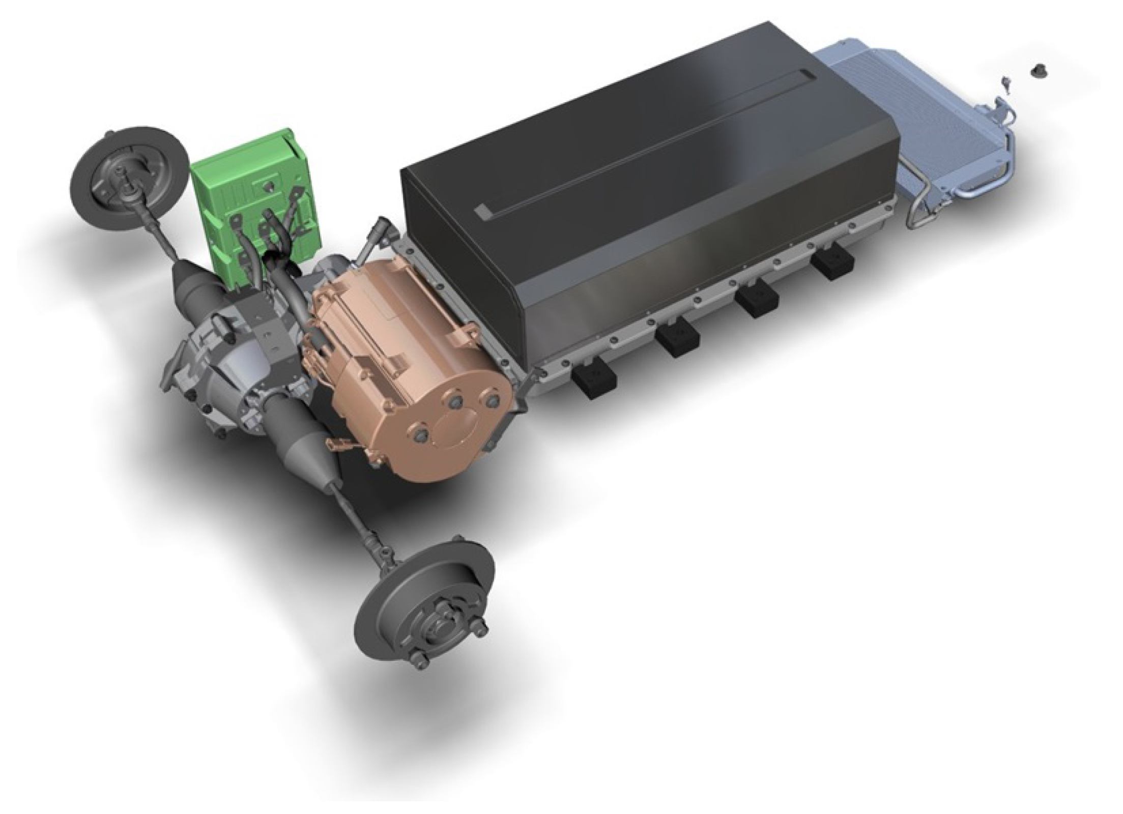
Figure 2 illustrates the electric powertrain of the Renault Twizy 80.
Figure 2.
Electric powertrain of Renault TWIZY 80.
This vehicle was also chosen because of the availability of extensive technical documentation. Indeed, the “Twizy Open Source P.O.M.” project [15], initiated by the vehicle’s manufacturer, has made a large amount of information publicly available. Additionally, several educational institutions have developed practical exercises based on this vehicle and documented their results [16,17]. As a consequence, high-quality data are accessible:
- Vehicle CAN Messagery: BMS, inverter, cluster.
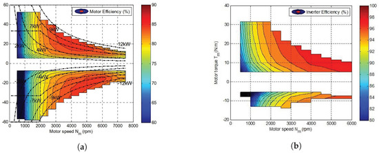
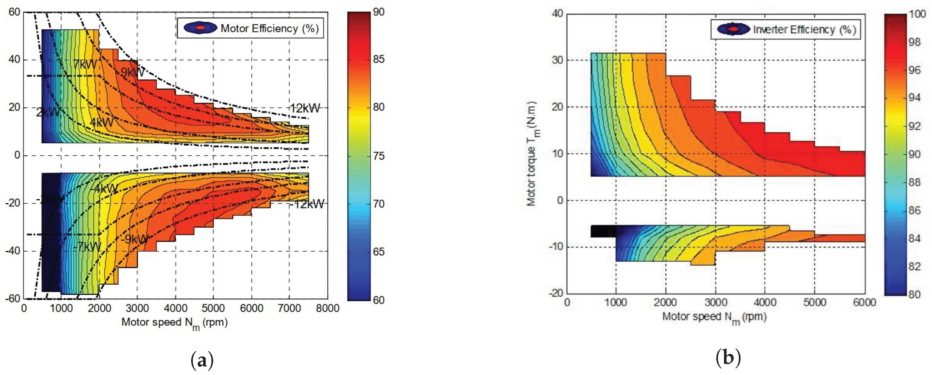
- Electric motor efficiency versus torque and speed (Figure 3a).
- Inverter efficiency versus torque and speed (Figure 3b).
Figure 3.
Manufacturer efficiency maps. (a) Motor efficiency map. (b) Inverter efficiency map.
Table A1 (Appendix B) gives the main characteristics of the Renault TWIZY 80.
3.2. Torque Meter
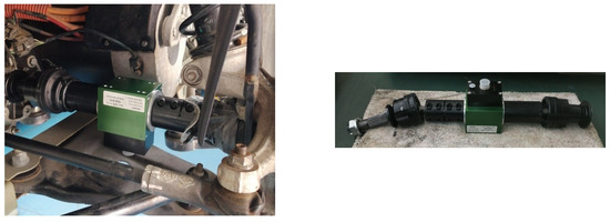
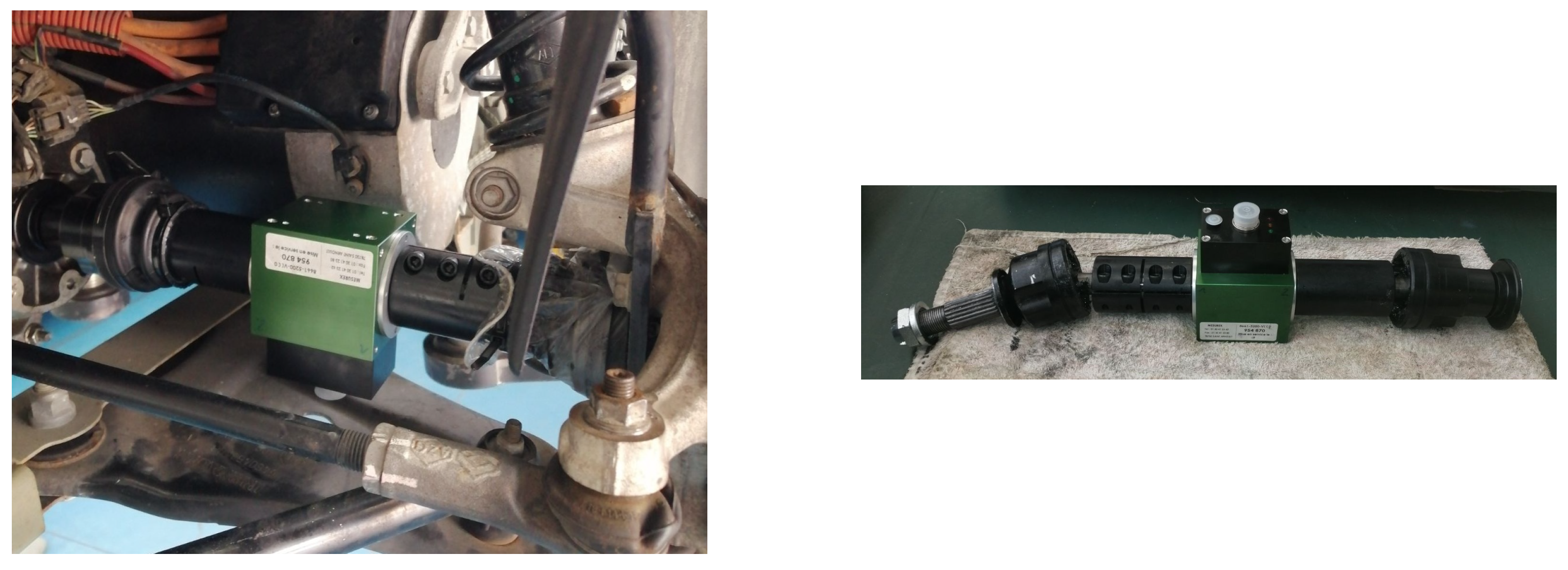
Figure 4 and Table A2 (Appendix B), respectively, gives a view of the selected torque meter and its specifications. Because it was not feasible to embed a rotary torque meter between the Induction Motor (IM) and the speed reducer, it has been chosen to place the torque meter between the speed reducer and the rim, on the right transmission shaft of the rear-driven car.
Figure 4.
Rotary torque meter installed on drive shaft.
3.3. Roller Test Bench
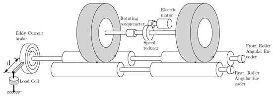
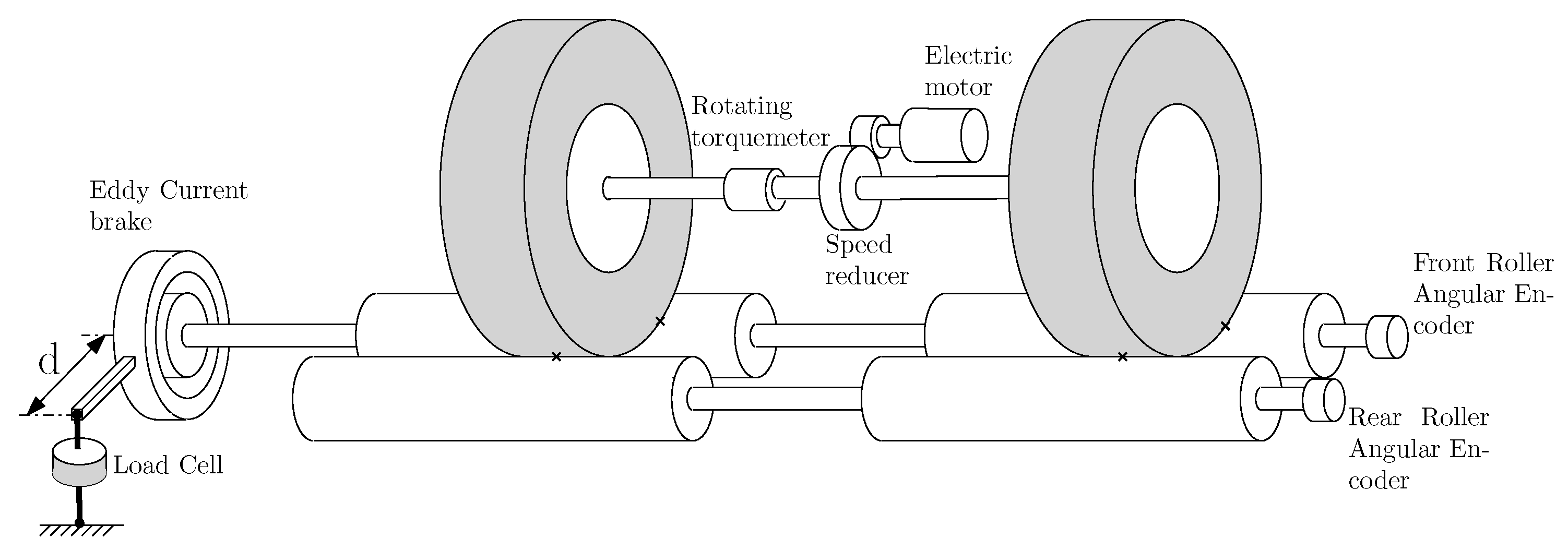
Figure 5 shows a simplified diagram of the roller test bench. The torques are measured at two different location: first at one driveshaft using the embedded torque meter, and second at the eddy current brake using a load cell. Moreover, it will be measured: battery voltage, battery current, and the several angular velocity sources—motor, drive shaft, and front and rear rollers.
Figure 5.
Overview diagram of the roller test bench.
Integrating a commercial rotary torque sensor into a drive shaft (see Figure 4) presents two main challenges: space constraints and potential mechanical weakening. The torque sensor requires sufficient space to accommodate the device itself along with its clamping systems at both ends. If space is limited, a smaller torque sensor may have to be used, which might not be able to cover the full expected torque range. Furthermore, this modification can lead to reduced mechanical strength or grip in the drive shaft, potentially preventing the transmission of the maximum expected torque. For these reasons, complementary measurements using a dynamo-meter at eddy current brake of the bench may be necessary to compensate for potential gaps in shaft-based torque measurement.
Table A3 gives the specifications of roller test bench used for this work.
The test rig is equipped with four rollers of the same radius . Each pair of front and rear rollers is rigidly coupled and connected to an angular encoder which will be used to determine the speed of rotation.
The eddy current brake acts only on the front roller line. The braking torque is measured in steady state condition, on the eddy current brake stator using a load cell placed at a distance d from the axis of rotation.
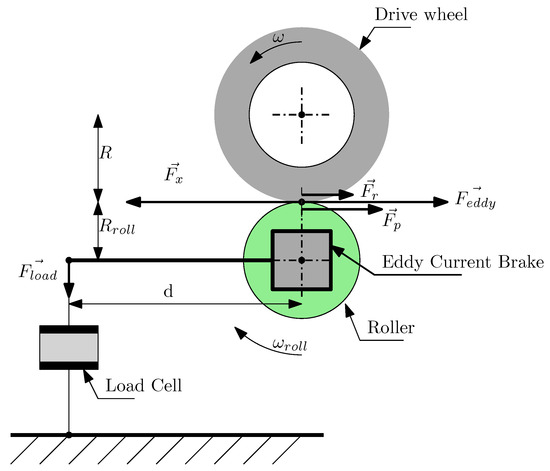
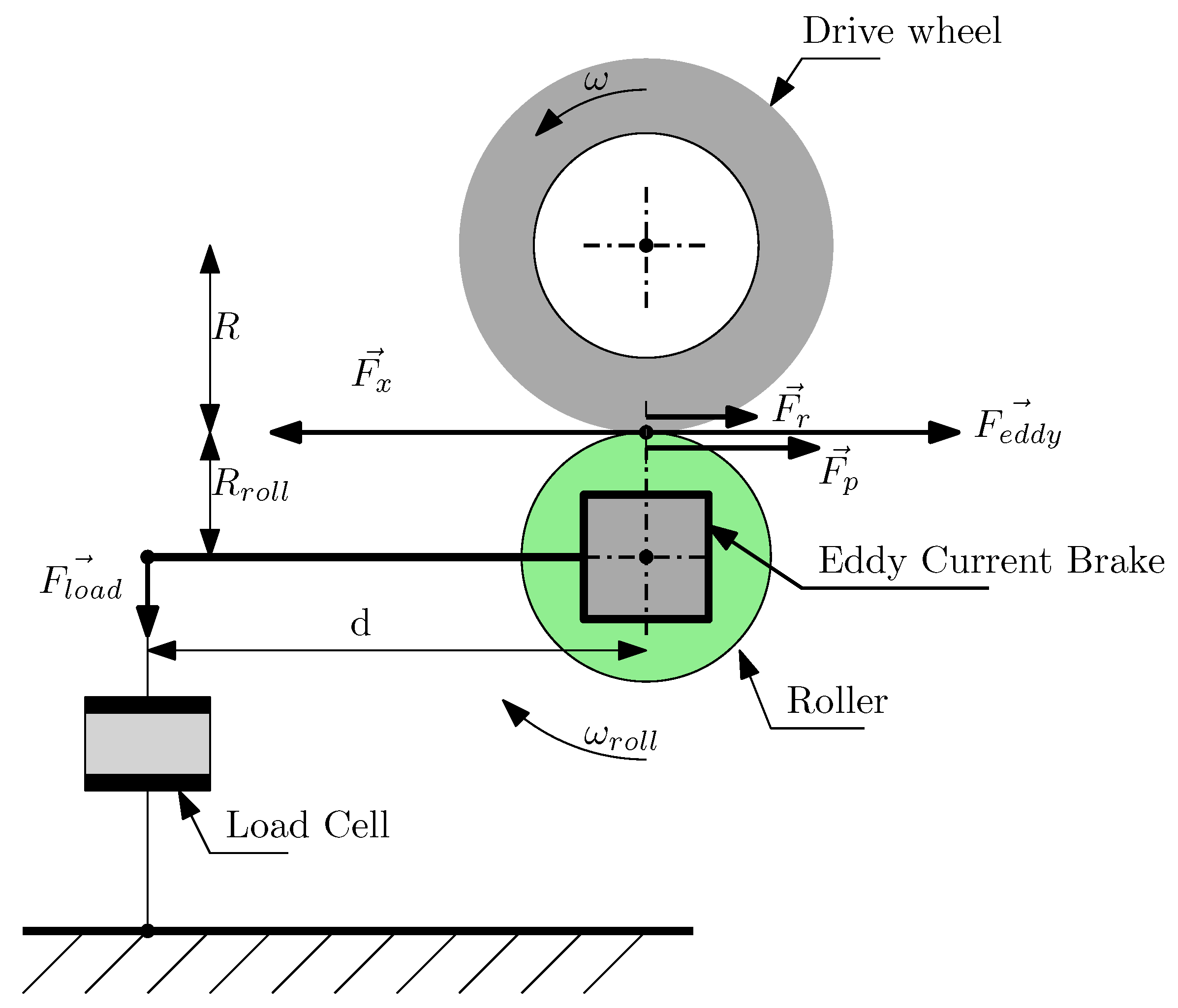
Figure 6 illustrates the forces acting to the vehicle when it is on the roller test bench.
Figure 6.
Force applied on drive wheel.
Equation (4) gives the vehicle law of motion on the roller bench. is the equivalent mass simulated by the rollers inertia and all rotating parts. This is discussed in a dedicated subsection below.
is the tangential speed on rollers or vehicle speed. is the driving force created by tire, is the resistant force created by the eddy current brake action, is the rolling resistance mainly due to the tire and finally is the intrinsic total resisting force of the rollers due to the frictional forces generated by the bearings supporting the rollers and the aerodynamic eddy current torque due to its inner ventilation.
is determined directly from the measurement of the applied force on load cell, denoted as (Figure 6):
Calculating correctly is a delicate operation, which is usually repeated several times. It depends on many factors, including temperature and rolling friction.
In the case where the roller test bench do not use a eddy current brake but a reversible electric motor, two methods are commonly used [12,18]: the constant resistance force method and the stationary points method. In both cases, the rollers are unloaded, meaning the weight applied on driven axle is not supported by the rollers. The calibration of frictional losses on the test bench is therefore not accurate: when the car rests on the rollers, the radial load generated by the weight of the axle alters bearing’s behavior.
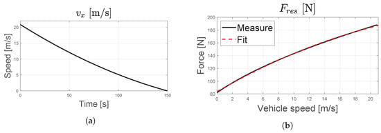
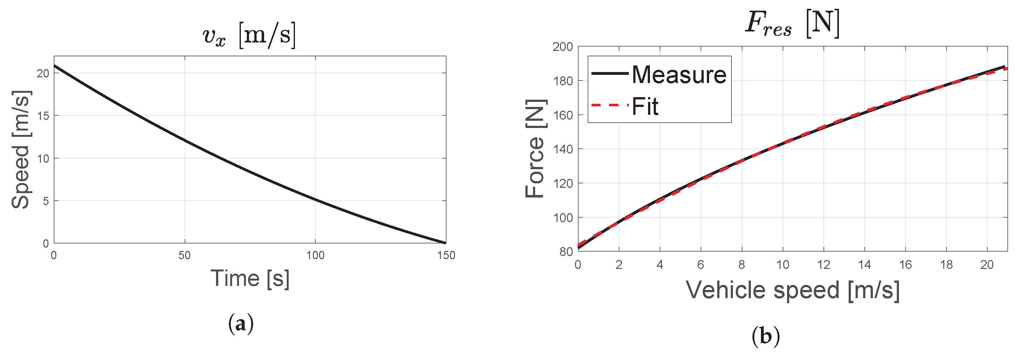
Since the test bench used in this study is not equipped with an electric motor and considering the objective of calibrating it under realistic load conditions, a deceleration-based method was adopted: The car is driven to the maximum speed allowed by the inverter with eddy current brake deactivated, ensuring that no resistant torque is applied to the rollers. The vehicle is then switched to neutral mode using the DNR selector in order to prevent any regenerative braking. The roller’s deceleration is then recorded without any action from the driver on the brakes or driving wheel. This method is known as the ‘coast down’ method [19].
During deceleration of the car, because the law of motion can be simplified as:
, defined as the total resistance force, is the sum of the resisting force of the roller due to friction forces and the rolling resistance force due to tire and transmission loss.
The drawback of the coast down method is that it is not possible to isolate and from . However, given the objective of the paper presented here, the authors consider this limitation to be inconsequential, as energy losses in tires due to rolling resistance are not taken into account in the efficiency mapping of a powertrain. Therefore, this method has the advantage of naturally excluding these losses.
Finally, the mechanical power dissipated by eddy current brake is given by:
3.3.1. Equivalent Mass
is the equivalent mass of the bench that provides a translation kinetic energy equal to the rotational kinetic energy of the rollers and rotating components in the vehicle’s transmission (such as the driveshaft, motor rotor, etc.).
is the rotational inertia of the rollers and J is the inertia of the rotating parts of the vehicle.
The tangential speed can be evaluated from both the roller and the wheel perspectives:
Determining J is not feasible without knowing the weight and dimensions of each rotating component, which may require complete disassembly of the vehicle. An alternative method for evaluating J is based on the work of [20,21]:
with m being the vehicle true static mass and the equivalent mass of the vehicle when taking into account the inertia of the rotating parts. The authors of Ref. [21] assume that is proportional as m and propose:
with a rotational inertia factor defined as:
where and are, respectively, the moment of inertia of the wheel associated with all rotating parts that moves with it (transmission shaft) and all rotating components associated with the power plant. and are, respectively, the gear ratio of the transmission and final drive. Finally the authors of Refs. [20,21] propose an empirical relation, valid for a passenger car, that takes into account the effect of wheels and the rest of transmission:
with G is the total gear reduction given by:
Using the previous equations, it is now possible to estimate J. The equivalent mass of the TWIZY was calculated to be 593 kg, which leads to a rotating inertia J of 8.48 kg·m2.
J has to be added to the roll inertia of the Rollers, according to Equation (10), to calculate the bench equivalent mass. Finally, a bench equivalent mass value of 970 [kg] is found.
3.3.2. Bench Calibration
Figure 7 gives the roller bench calibration results for the Twizy driven up to 80 km/h and then set in NEUTRAL mode. The resistant force has been classically fitted with a second degree polynomial function:
Figure 7.
Rolling resistance bench calibration. (a) Vehicle speed versus time. (b) Resistant force versus .
Table 1 gives the obtained coefficient, and correlation coefficient R2.
Table 1.
Resistant force fit results.
3.4. Electrical Power at Inverter Input
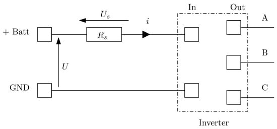
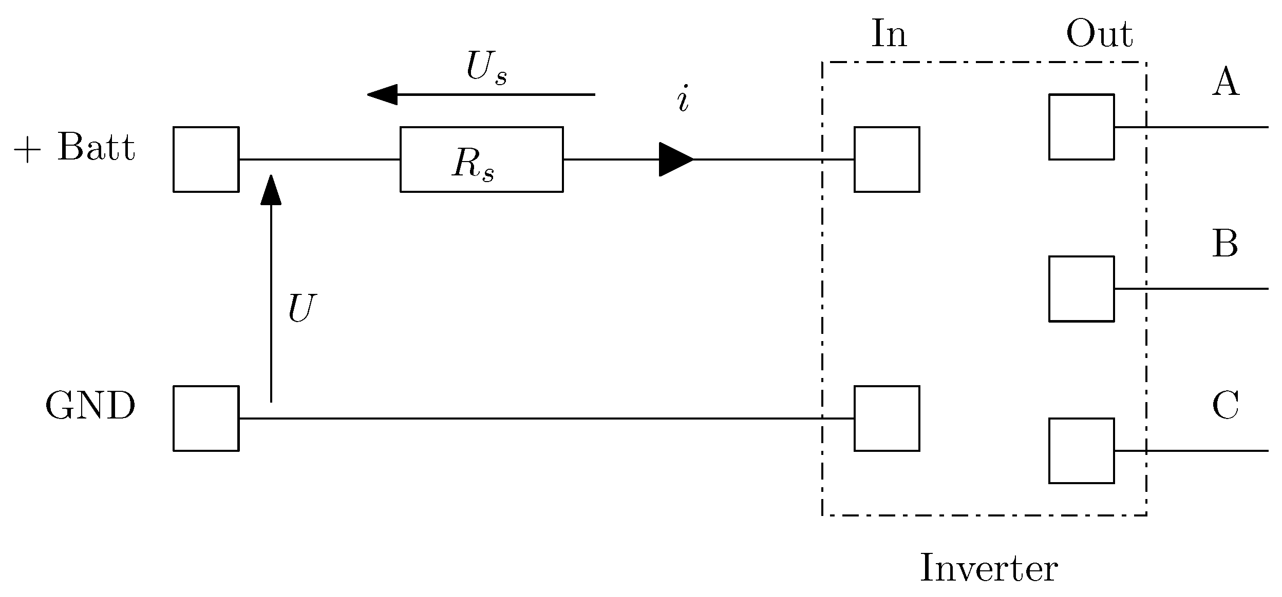
A second modification was made to the vehicle: the electrical circuit upstream of the inverter was opened to integrate an electric shunt required for current measurement.
Figure 8 depicts the electric power measurement at inverter input. is the shunt between battery and inverter input. U and are, respectively, the voltage at battery and shunt.
Figure 8.
Electric power at inverter input.
Because the current is pulsed, the inverter input power is calculated using acquisition data over n samples of the battery voltage and the shunt voltage, denoted and , respectively. For each sample, the instantaneous current is computed as .
This power is also evaluated using the data coming from the CAN messages emitted by the Battery Management System (BMS). These values are mean values calculated by the BMS, and are emitted each 30 ms: and , the mean battery voltage and mean battery current, respectively. This power is also evaluated using data obtained from CAN messages transmitted by the Battery Management System (BMS). These values are mean quantities computed by the BMS and transmitted every 30 ms: and , corresponding to the mean battery voltage and the mean battery current, respectively. Using these two quantities, the inverter input power can be calculated as:
These two methods have been used for a calibration process, and the results obtained have been very similar. For convenience, the experimental dataset was created using CAN messaging data.
3.5. Tire Longitudinal Slip
On a conventional roller test bench, the tire is part of the power transmission chain to the eddy current brake. Therefore, when estimating the wheel power from a power measurement taken at the brake, it is necessary to account for the power losses caused by longitudinal tire slip.
The phenomenon of longitudinal slip of a tire is well known and is a consequence of its viscoelastic nature. It results from the combination of two main effects. The first effect is the reduction in wheel’s effective radius when a torque is applied. This phenomenon is caused by the change in orientation of the carcass ply cords under motor torque. As a result, the cords tilt and are no longer aligned radially. This reduction in effective radius induces a virtual slip, meaning that it is not caused by an adhesion issue. The wheel’s rotational speed increases to compensate for the reduced radius, creating an apparent slip. The second effect is a real slip that occurs in the contact patch due to adhesion limit. This phenomenon is described, for instance, in Pacejka’s brush model [22,23,24].
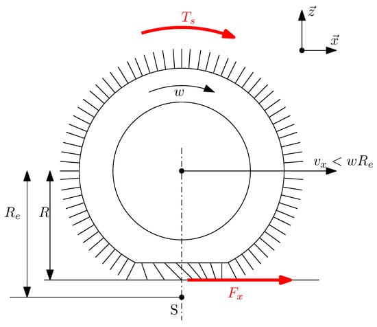
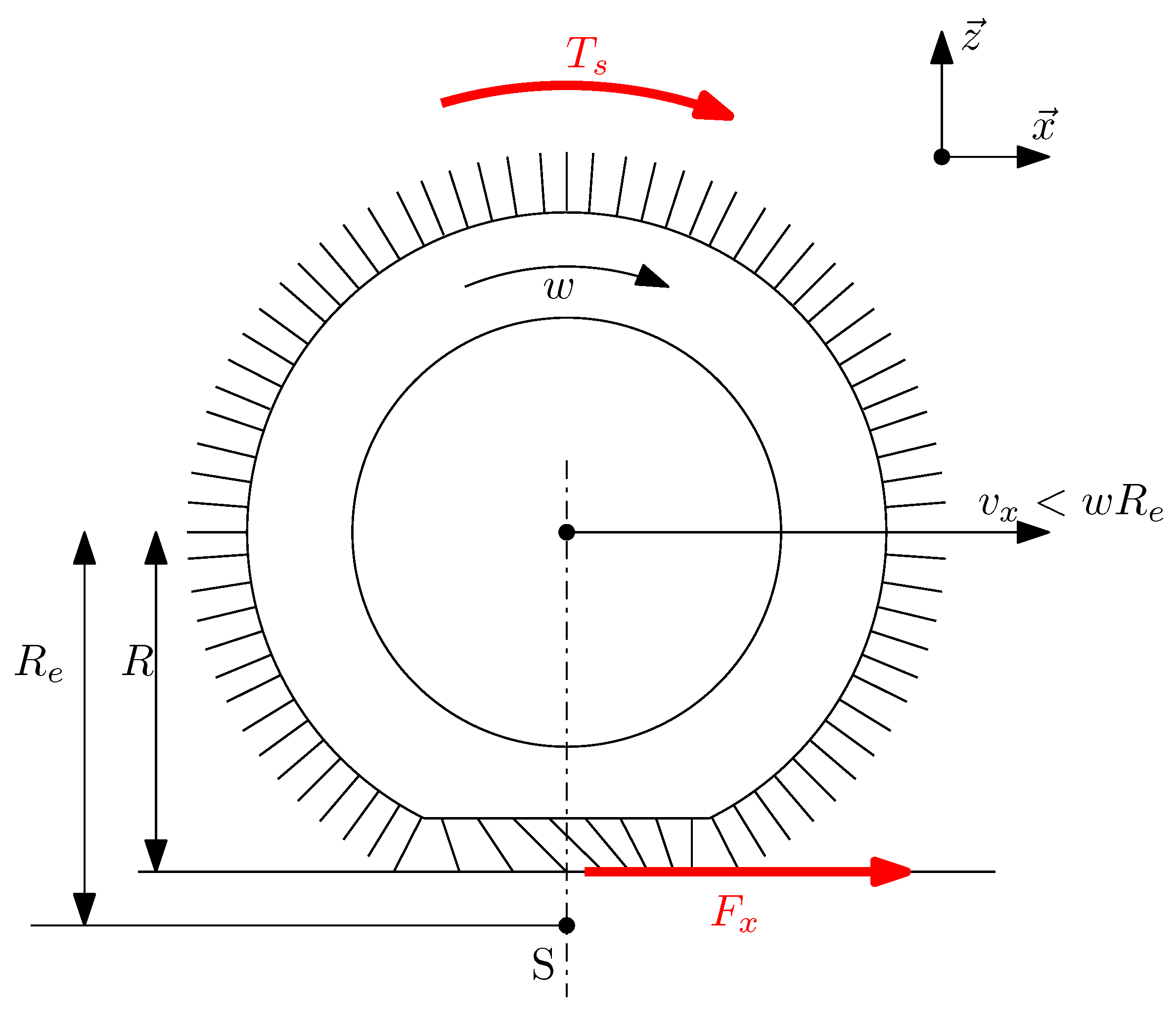
Figure 9 illustrates a driven wheel under vertical load. represents the torque applied to the rim by transmission shaft. is the tractive longitudinal force generated by the tire in reaction to the applied torque. denotes the angular velocity of the rim, while corresponds to the wheel’s longitudinal forward velocity.
Figure 9.
Tire in pure longitudinal slip conditions.
S is the slip point: it is a virtual point associated with the rim, located at a distance from the center of rotation. is the effective loaded radius of the tire. It is measured in a free-rolling condition, meaning no torque is applied to the rim. Finally, R is the effective radius of the wheel when a torque is applied. Due to two primary effects, R is smaller than : the radial deflection of the tire carcass and the deformation of tread blocks under applied forces (as described in the brush model).
is then defined as the angular velocity that would be observed if the wheel were in free-wheel condition.
The real angular velocity of the wheel is higher than due to tire deformation and real slip. It is posed as follows:
Next step is to define the sliding velocity as:
One can note that this sliding velocity is calculated from the one that should be observed in the free-wheel condition. The result is a higher slip speed than it would be calculated using the true radius of the wheel under torque. This overestimation of slip is performed for taking into account the real slip that occurs within the contact patch, in addition to the slip solely due to the tire’s geometric deformation.
The definition used for longitudinal slip, denoted as , differs from the one proposed by Pacejka [22]. It is an alternative definition employed by various authors, such as Sina et al. [23], for instance.
The latter definition will be used in the present paper, as it requires fewer assumptions in tire power modeling, as detailed below.
The longitudinal tire slip is determined on a roller test bench by comparing two angular velocity measurements: wheel and roller where the eddy current brake acts as . In the case illustrated in Figure 5, these are the front rollers. Typically, the angular velocity of the front rollers is lower than that of the rear rollers due to the tire relaxation occurring after passing over the resisting roller. The ideal velocity can then be calculated by considering the roller radius, :
Since the wheel is in equilibrium, it can be written, assuming that :
Let note the torque applied at the rim. The superscript ∗ indicates that this quantity is estimated, in accordance with the notation conventions adopted in this paper.
Using these quantities, it is possible to quantify the efficiency and power losses caused by the tire’s longitudinal slip phenomenon. The power supplied to the rim is given by:
The previous equation is defined for a single tire. If it is assumed that the same torque and angular velocity are applied at the second tire of the driven axle, then the total power transmitted to the tires is twice . In the remainder of this subsection, only one wheel is considered.
The power at tire output is given by:
The power loss in the tire, denoted , is expressed as:
The tire efficiency can then be expressed as:
3.6. Motor Torque
Since the torque at the electric motor output shaft, , is not directly measured, it is estimated from the known values of and the angular velocity by applying the principle of energy conservation and assuming that the total power is equally distributed between the two wheels of the driven axle.
The speed reducer imposes:
The motor torque is:
This simple scaling transformation using the gear ratio G, from (,) to (,) is necessary to express the maps in their conventional form—that is, it is referred to the motor side.
Nevertheless, the measured and modeled losses include those occurring in the speed reducer and therefore represent the total system losses, i.e., inverter + motor + speed reducer.
3.7. Loss Modeling
The graphical representation of losses and efficiency in an electric motor or drivetrain is commonly illustrated using a map based on two variables: torque and angular velocity .
It is typical to express the losses in an electric power plant as a polynomial function of the form [5,25]:
are the coefficients of the polynomial model, is the maximum degree of the polynomial with respect to the torque , and is the maximum degree of the polynomial with respect to the angular velocity .
This approach enables a physics-based modeling of losses and account for a broader range of physical factors. Each coefficient has one or several physical justification has explained by [20,26].
Authors such as Roshandel [5] suggest that a 3 × 3 matrix is sufficient for the coefficient to account for the various losses in an electric machine, including converter losses, conductive losses, iron losses, permanent magnet (PM) losses, mechanical losses, and transmission system losses.
In the following section, we will discuss and justify the dominant physical effects associated with each term of this matrix.
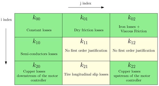
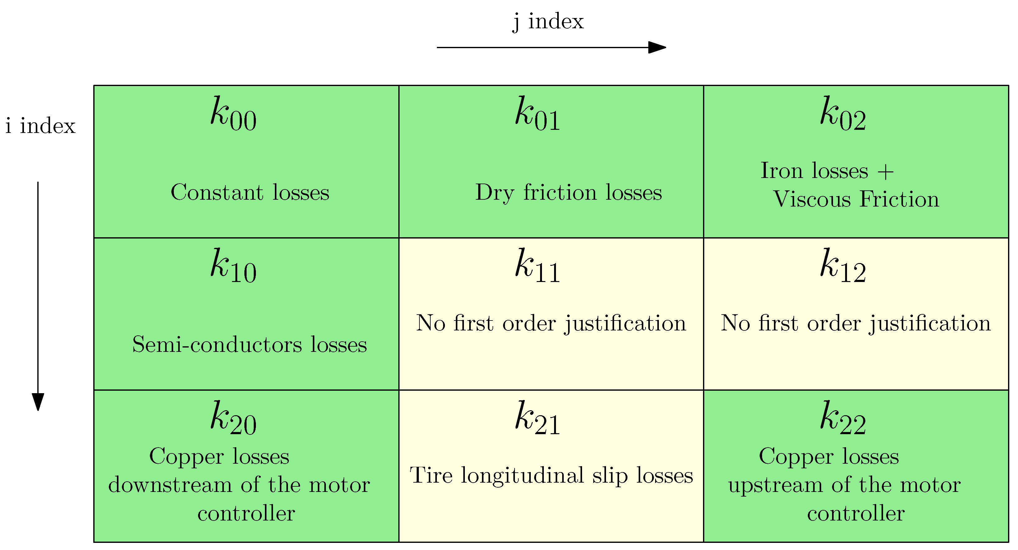
represents a constant loss of power not depending on or .
is physically justified by a constant dry friction force.
takes into account the viscous damping force and the iron losses [25].
typically takes into account the loss in the semiconductors of the inverter [26,27].
The coefficient is not commonly found in the literature. Firstly, it can be understood as a proportional loss to the output mechanical power . Roshandel [5] explains that this term can be introduced to account for second-order effects on additional Copper (Joule) losses in the constant torque region for an Induction Motor (IM). The term has no known first order physical basis, either in the literature or according to the authors’s understanding. This term can be introduced to account for second-order effects [5] in copper (Joule) loss and iron loss for an IM motor. According to author’s aim to take into account only first order factor, both coefficients and will not be used.
The coefficient corresponds to the well-known copper (Joule) losses. Since torque T is proportional to current i, and copper losses scale with , this term has a strong physically justification.
The term may be used to account for longitudinal tire losses, if necessary. The power loss in the tire can be expressed as , with that is proportional to torque or , and . Thus, tire power losses can be modeled as being proportional to . However, in this paper, because tire losses are out of the scope of the efficiency map, this term will not be used.
Finally, the coefficient is not referenced in the literature, excepted to account for second order factors. The authors propose to retain it in order to represent copper losses occurring upstream of the inverter. Indeed, if we assume that the mechanical power is equal to the electrical power (with unit efficiency), one can write: where and are, respectively, the supply current to the inverter and the battery pack voltage.
Assuming the battery voltage is almost a constant, it follows that the current is proportional to the product . Now, the copper (Joule) losses upstream of the inverter are scaled to . Therefore, these losses are proportional to the product .
Figure 10 summarizes this discussion, with a color convention as follows:
Figure 10.
Physical representation of polynomial parameters for power loss modeling.
- A green background indicates a factor with a physical justification and a first-order effect on losses. Therefore, it is included in the least-squares fitting process.
- A yellow background indicates a factor with either a negligible first-order effect on losses or one that falls outside the scope of losses considered by the authors.
3.8. Unconstrained and Constrained Least-Squares Fitting
It is considered an experimental data triplet consisting of the three quantities , or alternatively if the measurements are obtained, respectively, from the torque meter or from the brake load cell. The index i refers to the triplet under consideration within the complete set of n triplets. In the remainder of this paper, the methodology will be illustrated using the experimental triplet .
As a first step, we construct a triplet of dimensionless values, denoted , defined as follows:
The least-squares method can then be applied using matrix notation [28]:
where denotes the vector containing the dimensionless estimated power losses obtained by least-squares method, Q is the regressor matrix, K is the vector of parameters to be estimated, and is the vector of residual errors:
According to least-squares theory, the K vector can be determined as:
When applying this basic method, a vector K containing 9 values is produced, some of which may potentially be negative. This technique will hereafter be referred as the “unconstrained” method.
A second approach, referred to as the “constrained” method, consists of enforcing all coefficients to be strictly positive or zero. Consequently, any fit that results in any negative coefficient is rejected. For example, one can perform a new fit after removing the column associated with the negative coefficient in the Q regressor matrix and associated raw the K vector, or use a dedicated constrained least-squares function.
This constraint is not systematically applied in the literature: some authors allow negative coefficients to enhance the quality of the fit, although this affects physical interpretability. It will be discussed in detail in Section 4.2.
3.9. Verification of Underfitting and Overfitting
In any data-fitting technique, the model may be subject to overfitting or underfitting.
In order to ensure the quality of the fit obtained using the least square method, a classical technique known as K-fold cross-validation was employed [29].
The experimental dataset, consisting of 78 data points, was randomly divided into 6 subsets of 13 values each. For each of the 6 combinations, a least-squares fit was performed using 5 subsets as the training set, while the remaining subset was used as the validation set.
The absence of underfitting is assessed by verifying that the mean of the residuals, denoted as is close to zero, indicating that no systematic information remains unmodelled.
The risk of overfitting is evaluated using a accuracy indicator, chosen here as the RMSE (Root Mean Square Error). It is verified that RMSE values obtained for each of the 6 cross-validation combinations are comparable, indicating good generalization capability of the model.
Once these two conditions are satisfied, a final fit is performed on the entire dataset (78 data points). The overall RMSE and the final mean of the residuals are then computed to characterize the final performance of the model.
4. Results
4.1. Raw Measurements
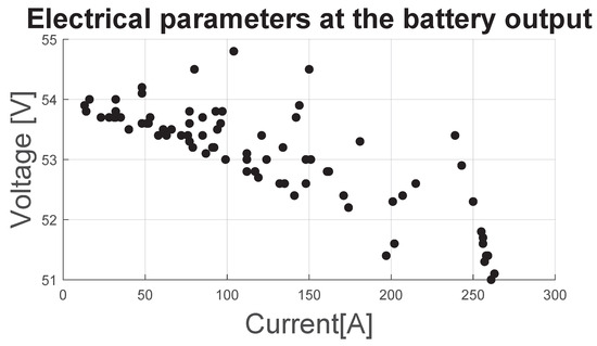
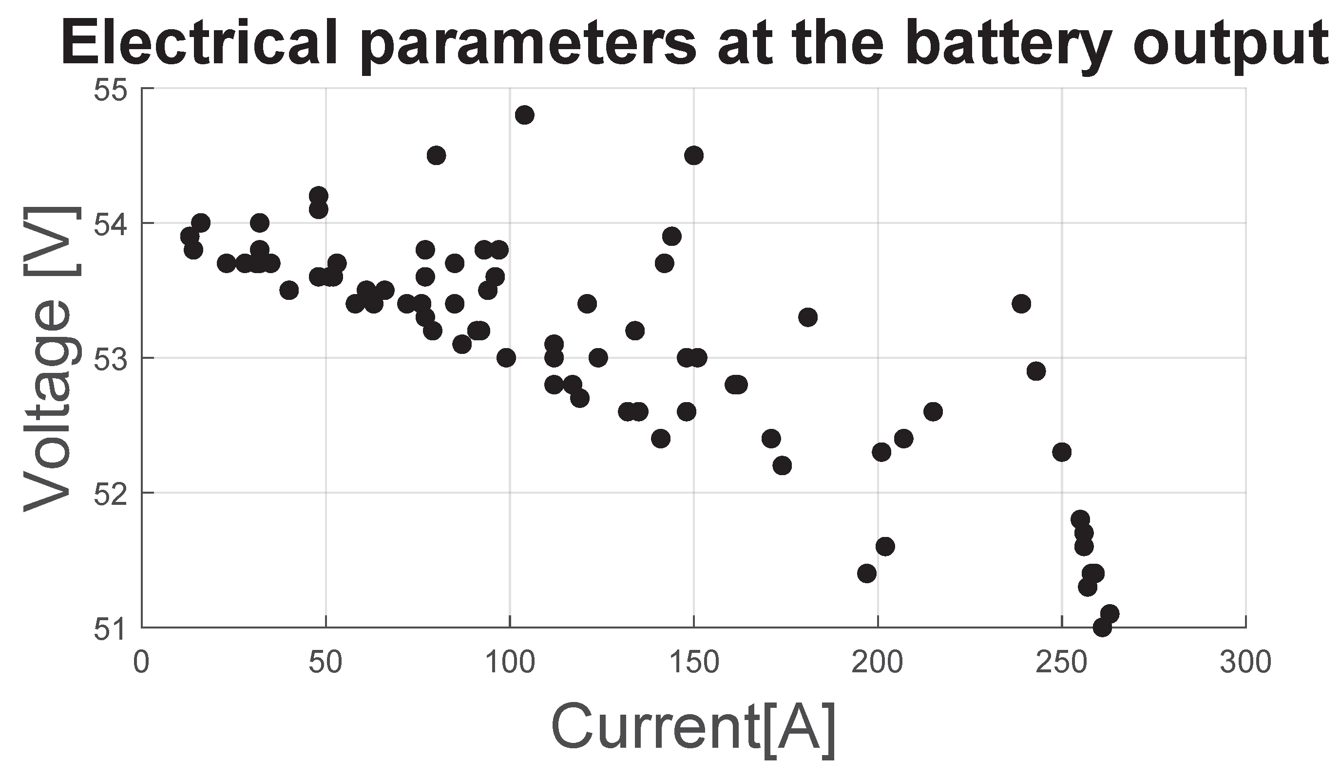
Figure 11 shows the 78 recorded measurement points, corresponding to the electrical parameters at the battery output: and . It can be observed that the battery output current can reach very high values, up to 263 A, which is fully representative of the conditions encountered in an standard electric vehicle under full load. Here, the battery voltage ranges between 54.8 V and 51 V.
Figure 11.
Battery voltage versus current.
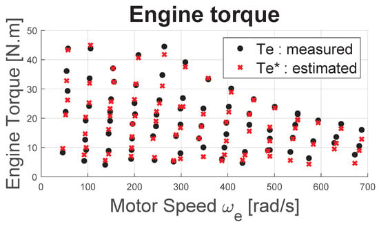
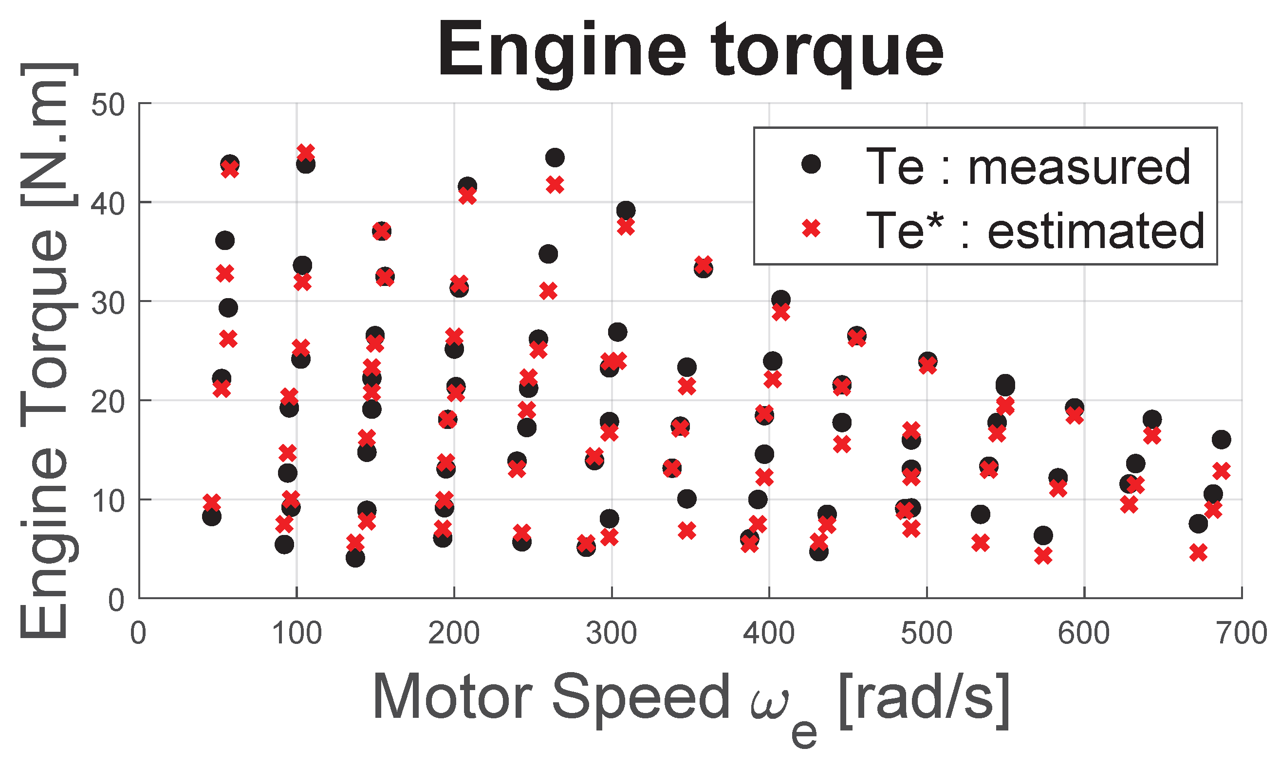
Figure 12 shows the 78 recorded measurement points, corresponding to the torque and motor speed pairs (, ) as well as the (, ) values. These measurements effectively cover the entire operating range of the motor. Additionally, the evolution of the maximum torque versus motor speed is typical of an electric motor. It is observed that the maximum measured torque is 48 N·m, which is lower than the manufacturer’s specified value of 57 N·m, likely due to an inverter limitation.
Figure 12.
Torque and RPM dataset.
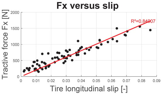
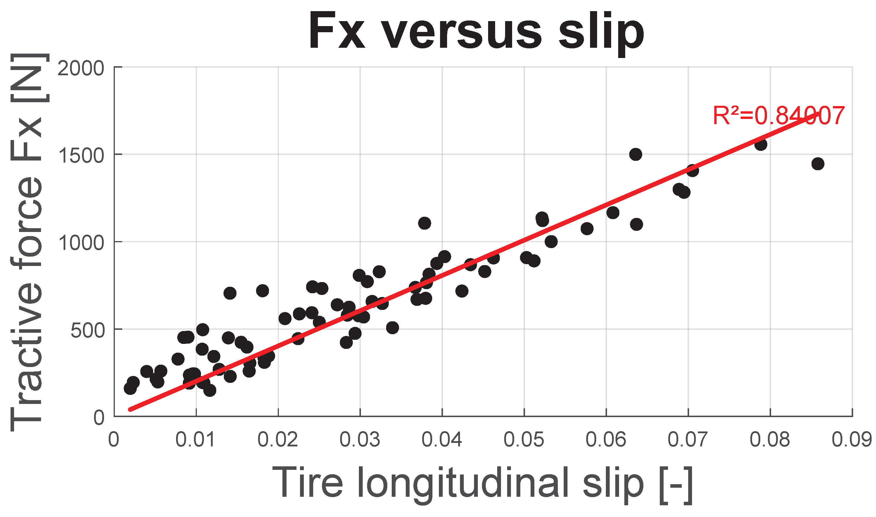
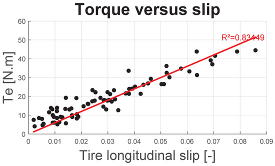
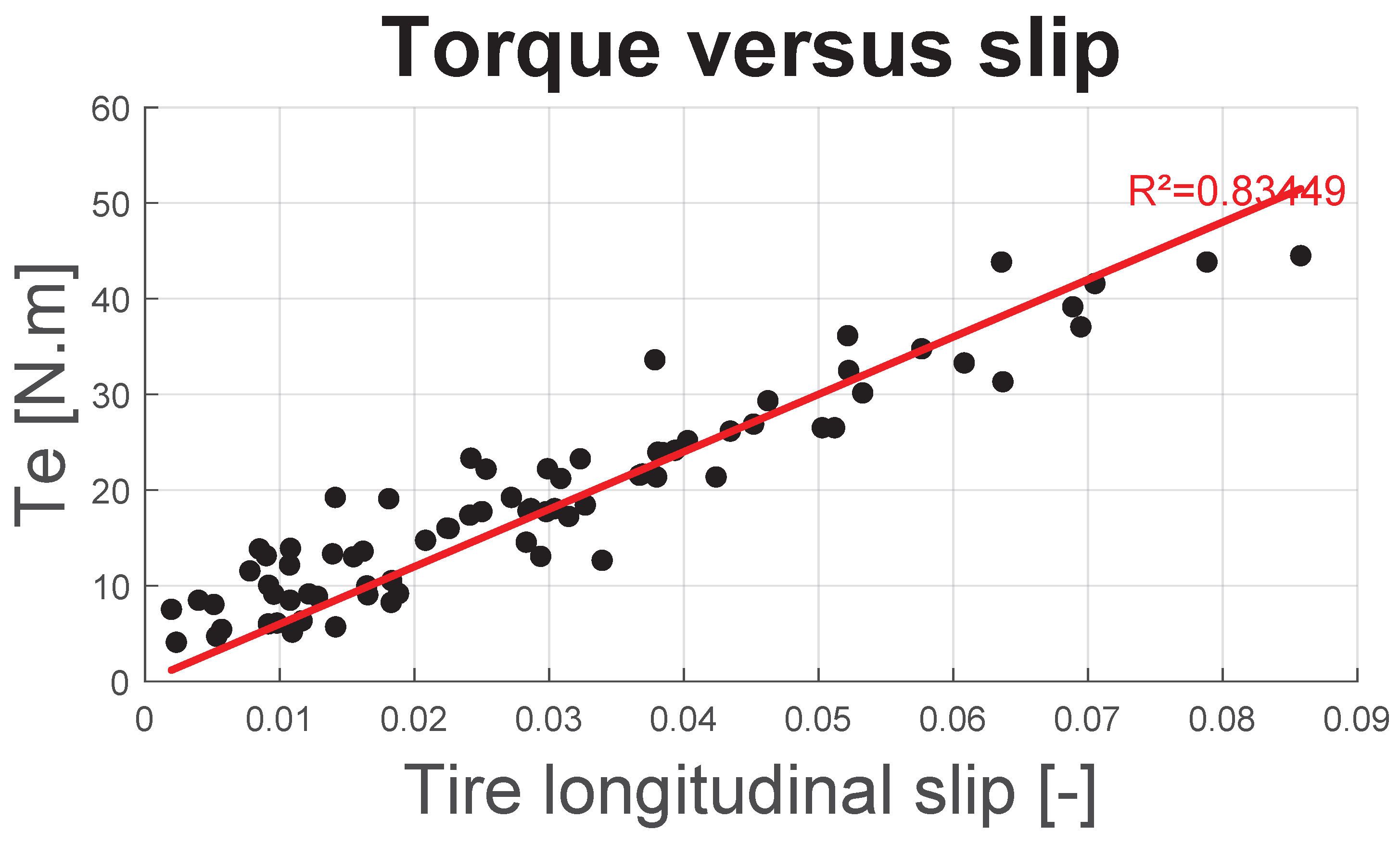
Figure 13 and Figure 14, respectively, depict the total motor force transmitted by both tires and motor torque as a function of longitudinal slip. As expected, the force increases proportionally with slip, despite a relatively low correlation coefficient. This linear behavior suggests that the adhesion limit has not been approached or reached. Consequently, the use of the slip-induced power loss model defined in Equation (27) remains valid.
Figure 13.
Motor force as function of .
Figure 14.
Torque, Te, as function of .
Figure 13 highlights a variation of approximately ±250 N around the value estimated by linear regression. Such a level of uncertainty is commonly observed in experimental vehicle measurements [30,31] or is adopted as white noise in simulations aiming to replicate realistic behavior under real-world conditions [24].
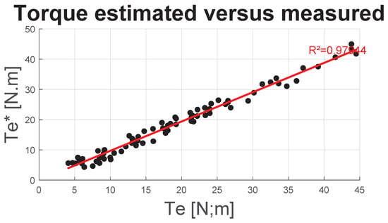
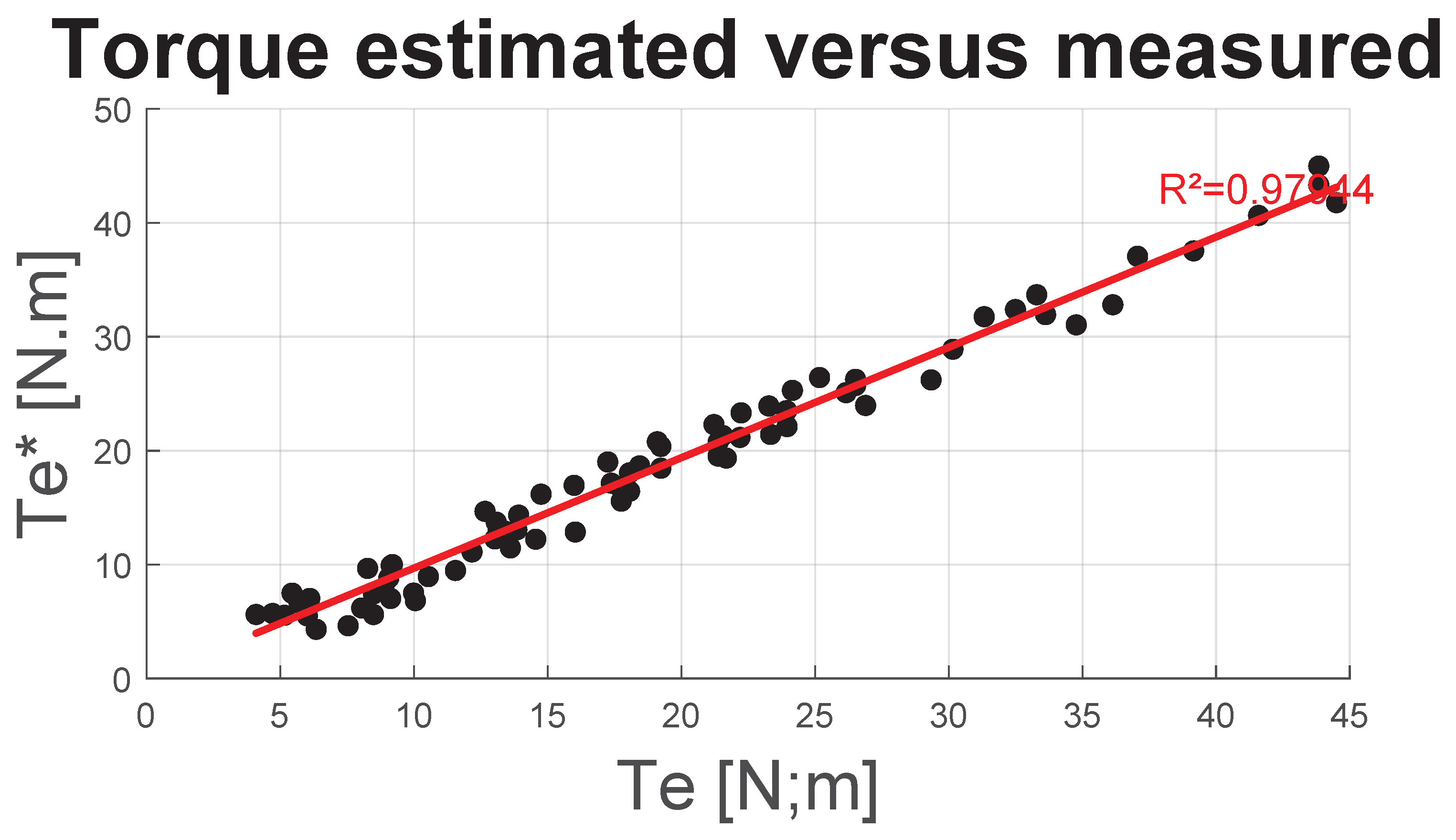
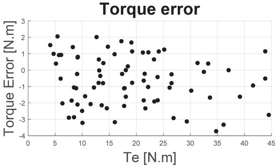
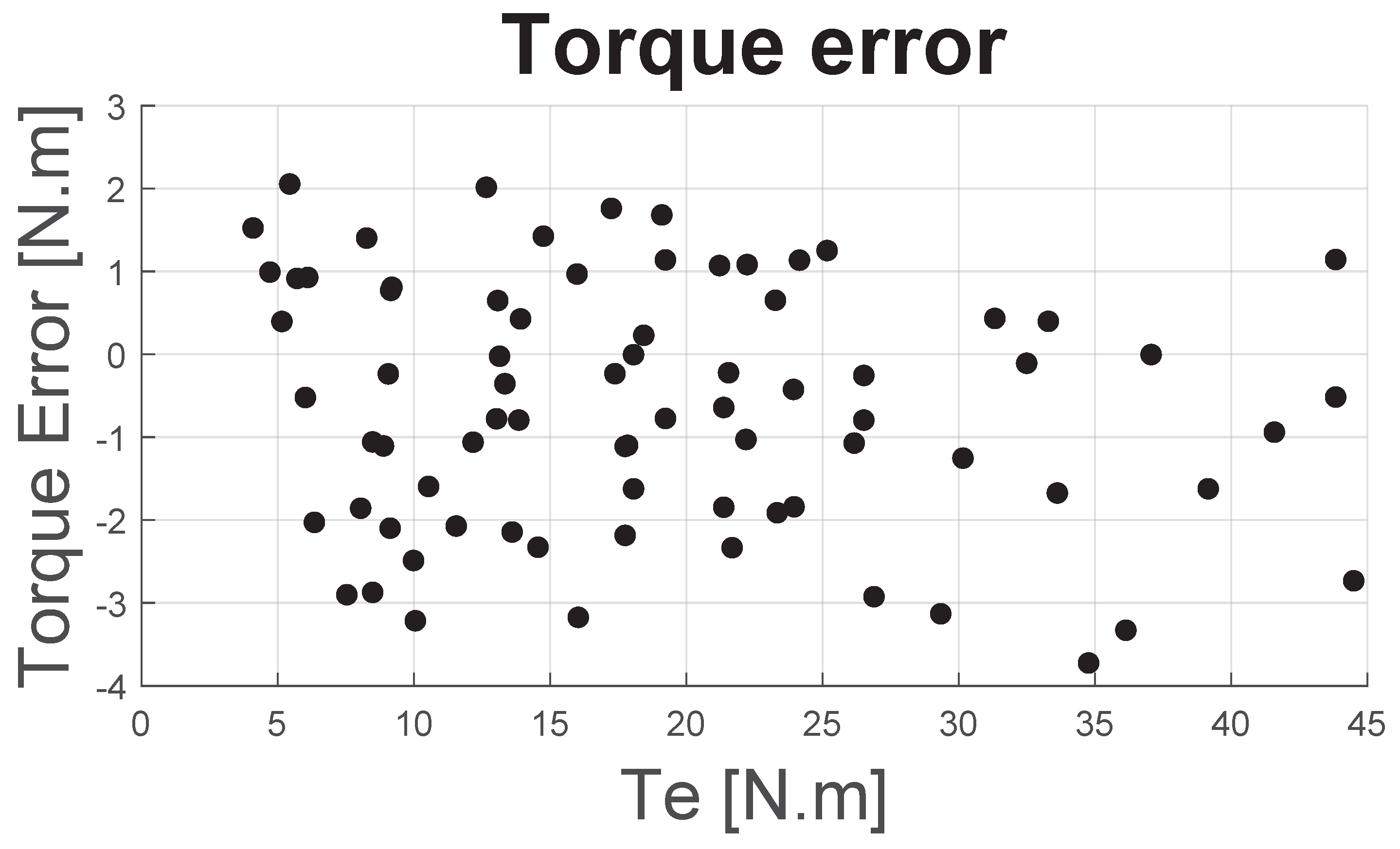
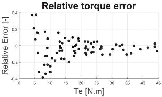
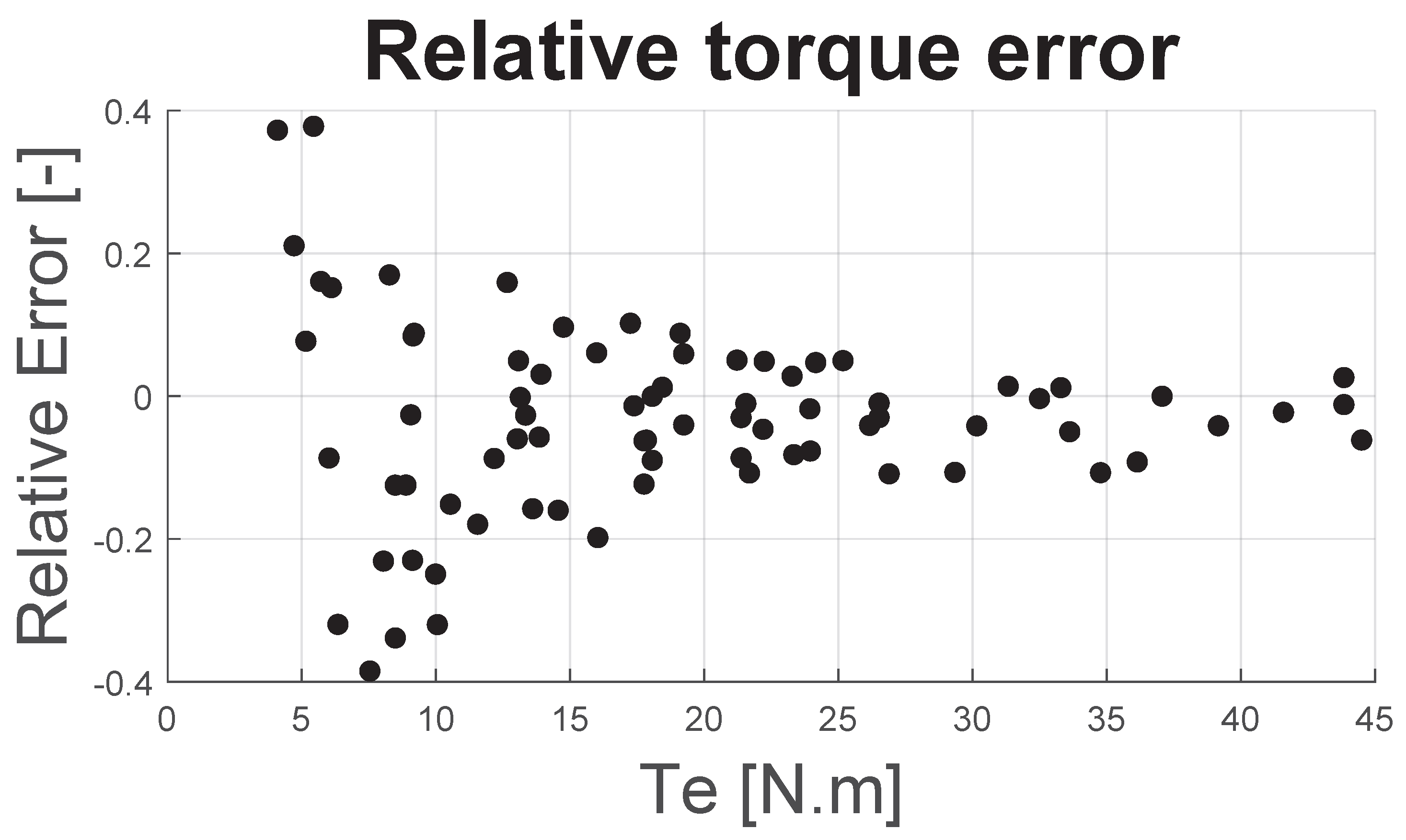
Figure 15 shows the estimated motor torque as a function of the measured motor torque . Figure 16 and Figure 17 present, respectively, the torque error and the relative torque error , both plotted against .
Figure 15.
as function of .
Figure 16.
Torque error as function of Te.
Figure 17.
Relative torque error as function of Te.
Figure 15 shows that the correlation between the estimated torque and the measured torque is almost satisfactory. Figure 16 indicates that the torque error remains within ±2 N·m, regardless of the value of . More importantly, this figure suggests that there is no significant bias, such as improper calibration of the test bench’s resistant force or inaccurate estimation of the tire’s unloaded radius . The observed error is therefore primarily attributed to measurement uncertainties, notably those related to the brake load cell and the estimation of tire longitudinal slip.
As a result, Figure 17 shows that the relative error, for torque levels above 20 N·m, remains within ±10%, which is generally considered acceptable for this type of measurement.
This is an important result as it indicates that if the torque and consequently the tire slip is too low (in this case, , as shown in Figure 14), then the torque estimation without a rotary torque meter is not reliable.
4.2. Data Fit Results
A least-squares fitting procedure was applied to the dataset of 78 measurement triplets and . The model was validated using the K-fold cross-validation method, as previously described.
For each measurement dataset (torque meter and brake-based), an initial fit—referred to as ‘unconstrained’ fit—was performed using all 9 coefficients of the matrix, allowing the coefficients to take on negative values.
Subsequently, a second fit—referred to as ‘constrained’ fit—was carried out, in which undesired terms () or those lacking first-order physical justification (, ) were excluded from the fitting process. Any negative coefficient resulting from the fit triggers a new iteration, during which the associated regressors (corresponding to the negative ) are removed, until only positive coefficients remain.
Table 2 summarizes the fitted coefficients , the Root Mean Square Error (RMSE) and the mean value of the residuals obtained for both models and both measuring techniques.
Table 2.
Data Fitting Results.
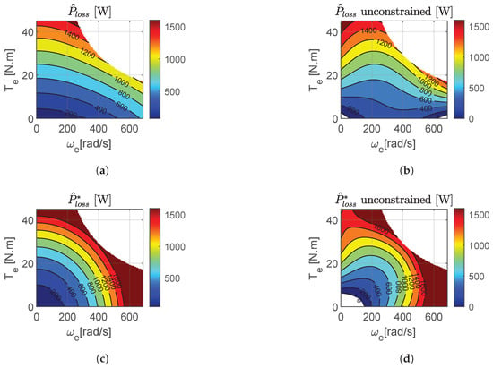
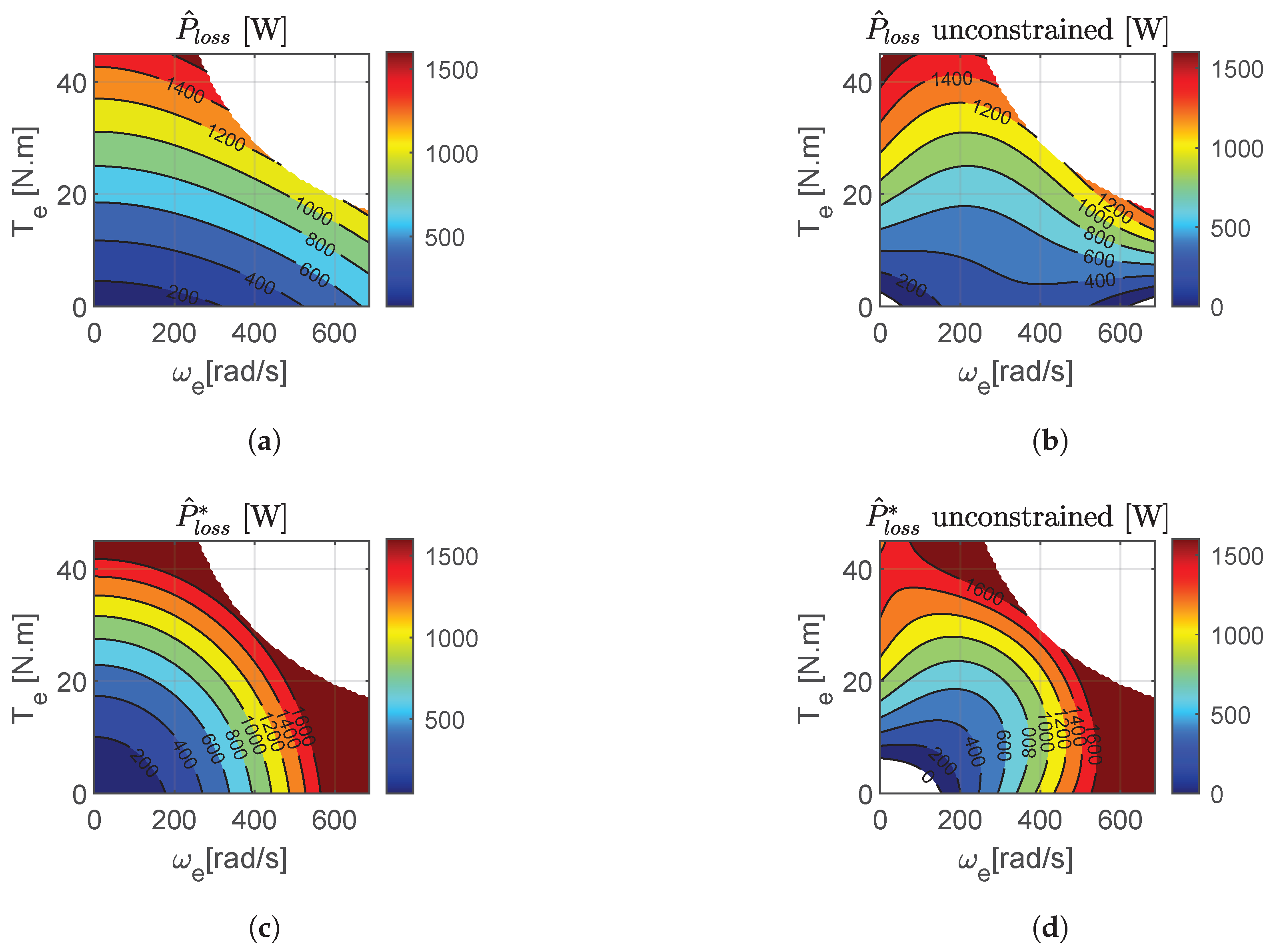
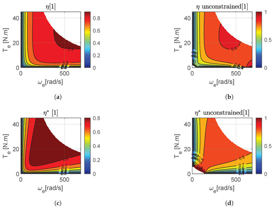
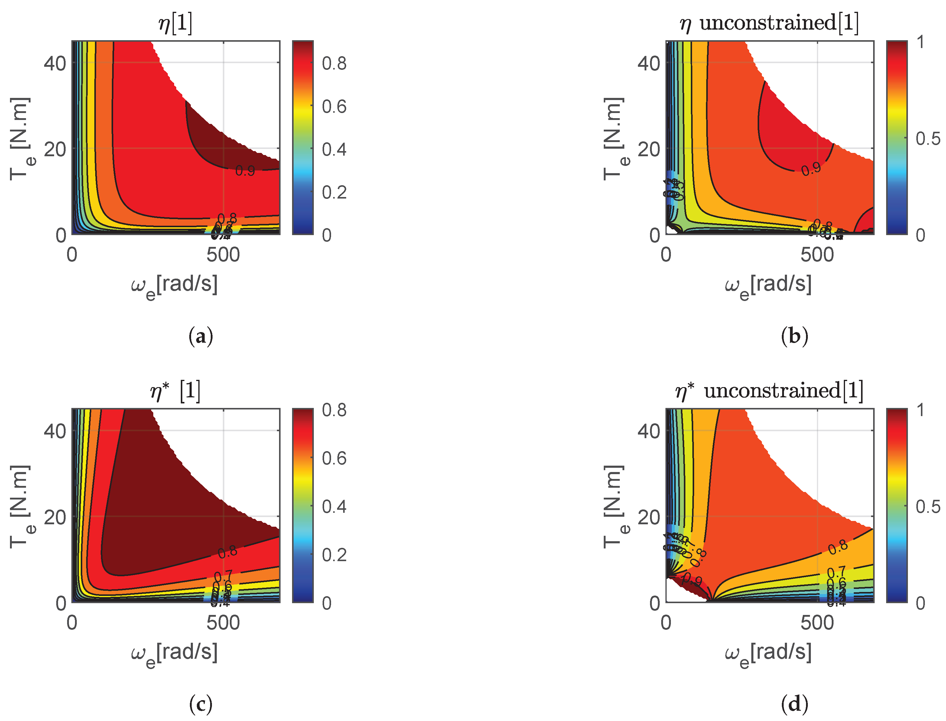
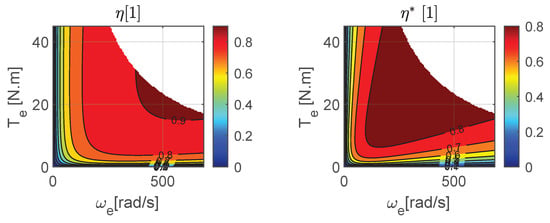
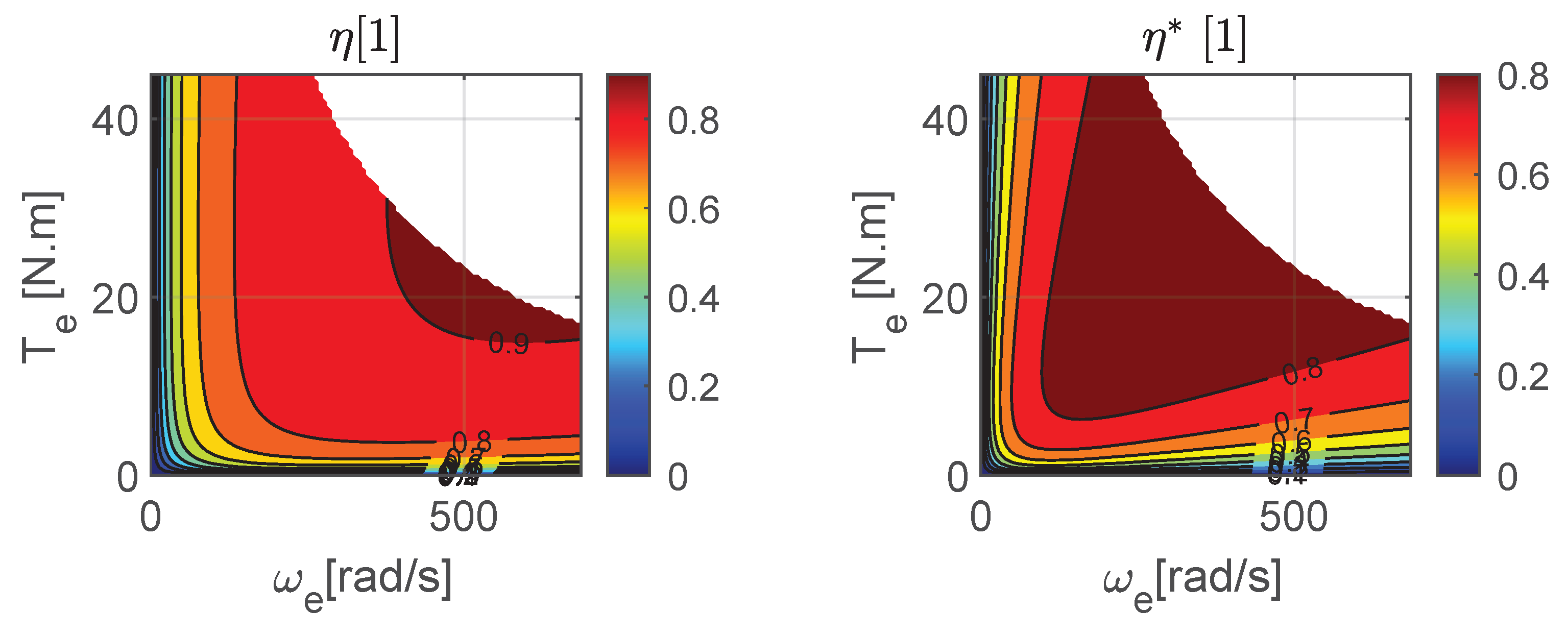
Figure 18 presents the predicted power loss maps, and , obtained using both fitting techniques (“constrained” and “unconstrained”) for both datasets (torque-meter-based and brake-based). Figure 19 gives the predicted efficiencies.
Figure 18.
Predicted overall losses. (a) Constrained fit for torque meter measurements. (b) Unconstrained fit for torque meter measurements. (c) Constrained fit for brake-based measurements. (d) Unconstrained fit for brake-based measurements.
Figure 19.
Predicted efficiencies. (a) Constrained fit for torque meter measurements. (b) Unconstrained fit for torque meter measurements. (c) Constrained fit for brake-based measurements. (d) Unconstrained fit for brake-based measurements.
5. Discussion
5.1. Discussion on the ‘Constrained’ and ‘Unconstrained’ Fitting Techniques
First, the ‘unconstrained’ fitting technique must be assessed. The fact that this method produces negative coefficients raises two major issues.
The first issue is that, in order to improve the fit quality, the ‘unconstrained’ method tends to overestimate certain physical losses associated with positive coefficients, while compensating by introducing negative values. As a result, the coefficients become difficult to interpret, making it impossible to compare different powertrain configurations.
The second issue is that these negative coefficients can lead to negative power loss values or efficiency values greater than 1 in certain areas of the maps. These invalid points must therefore be removed, which creates gaps in the maps. Such areas are clearly visible in Figure 18 in the lower left and right parts of plot (b), and in the lower left area of plot (d).
This problem does not occur with the ‘constrained’ method, whose maps are much smoother and more continuous. The RMSE analysis (Table 2) also shows that applying the ‘constrained’ method only slightly reduces the fit accuracy. For these reasons, the authors consider the ‘constrained’ technique to be the only suitable approach and it will be used for the analysis presented in the remainder of this paper.
5.2. Discussion on the Results
First, it should be noted that the obtained efficiency maps show good agreement with the expected results for AC motors, as described by [32,33], as well as with the data provided by the vehicle manufacturer (Figure 3).
A difference can be observed between the two fitted models (Table 2): the dataset obtained using brake measurements yields a zero value for the coefficient , whereas the dataset based on torque sensor results in a non-zero value for the same coefficient. Additionally, the coefficients obtained from each fitting procedure differ significantly.
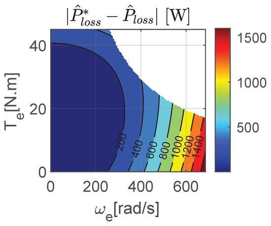
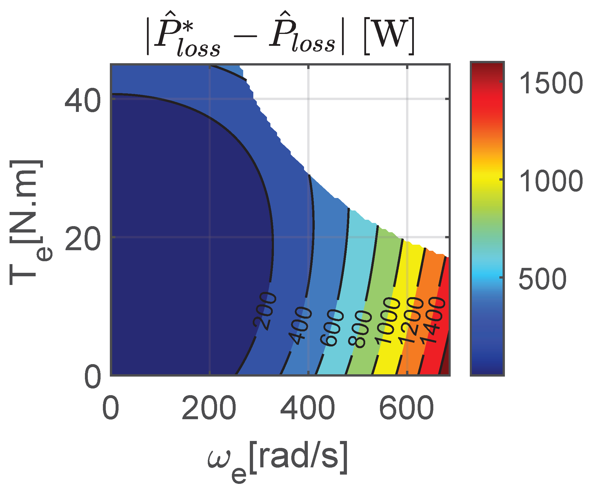
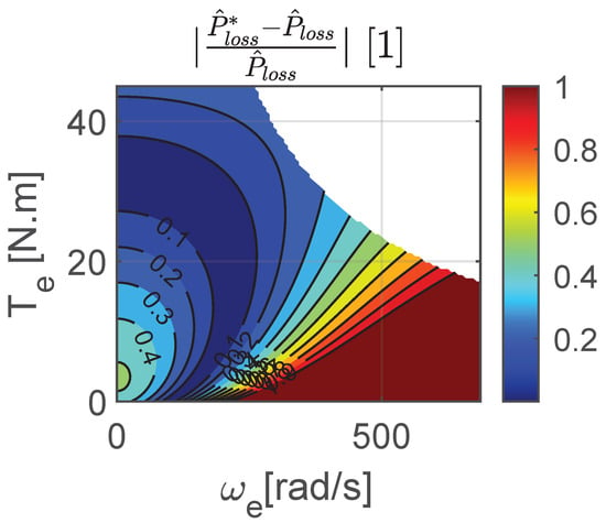
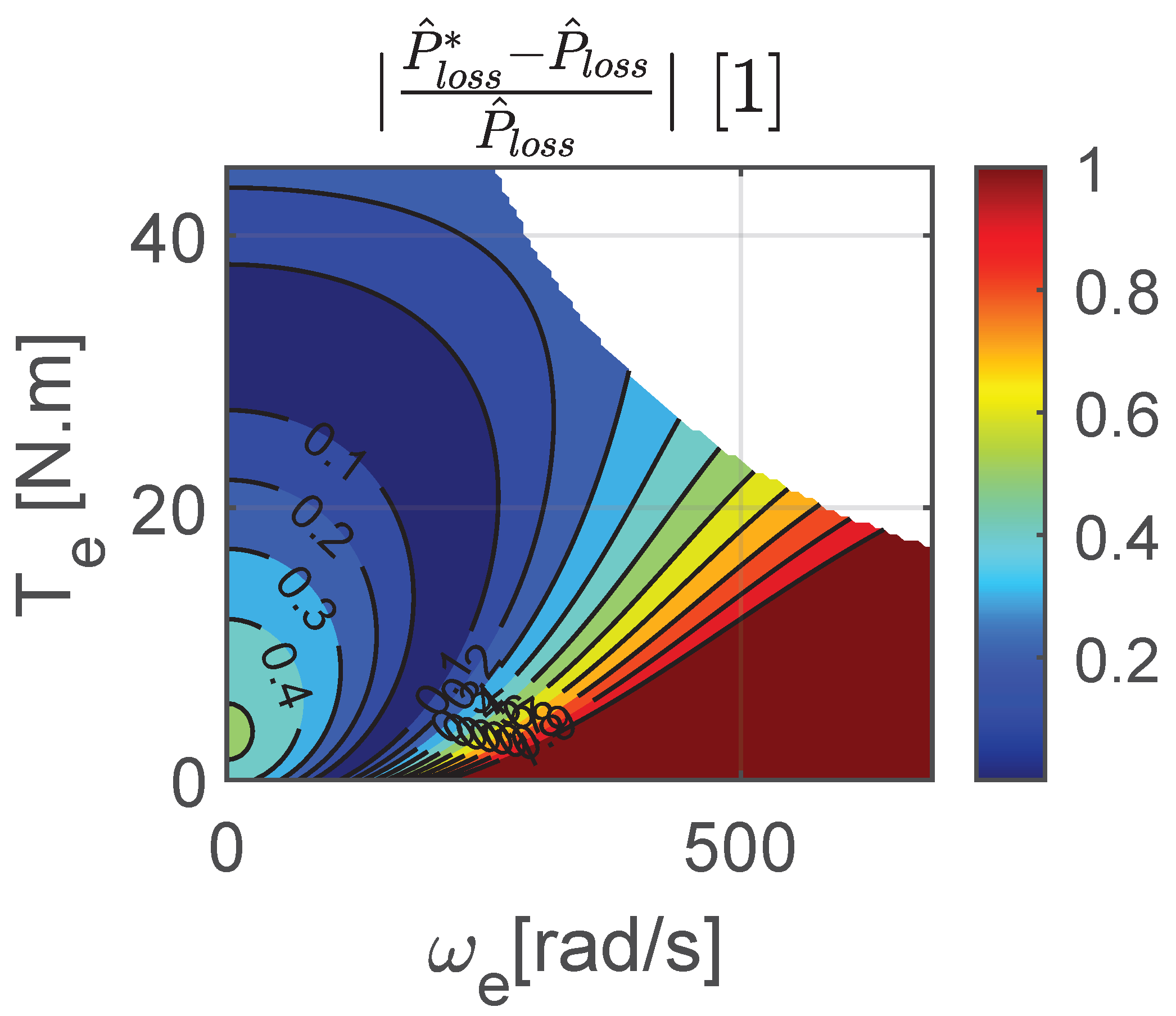
Figure 20 gives the graphical representation of the absolute power losses error defined as . Figure 21 gives the graphical representation of the relative power loss error defined as .
Figure 20.
Absolute power loss error.
Figure 21.
Relative power loss error.
These figures further highlight that the model based on brake measurements predicts greater power losses at high rotational speeds compared to the model derived from torque meter. Figure 21 clearly shows that the relative error remains acceptable for high torque values. This observation is consistent with the findings discussed earlier in the section on raw measurements.
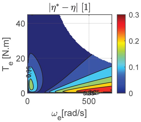
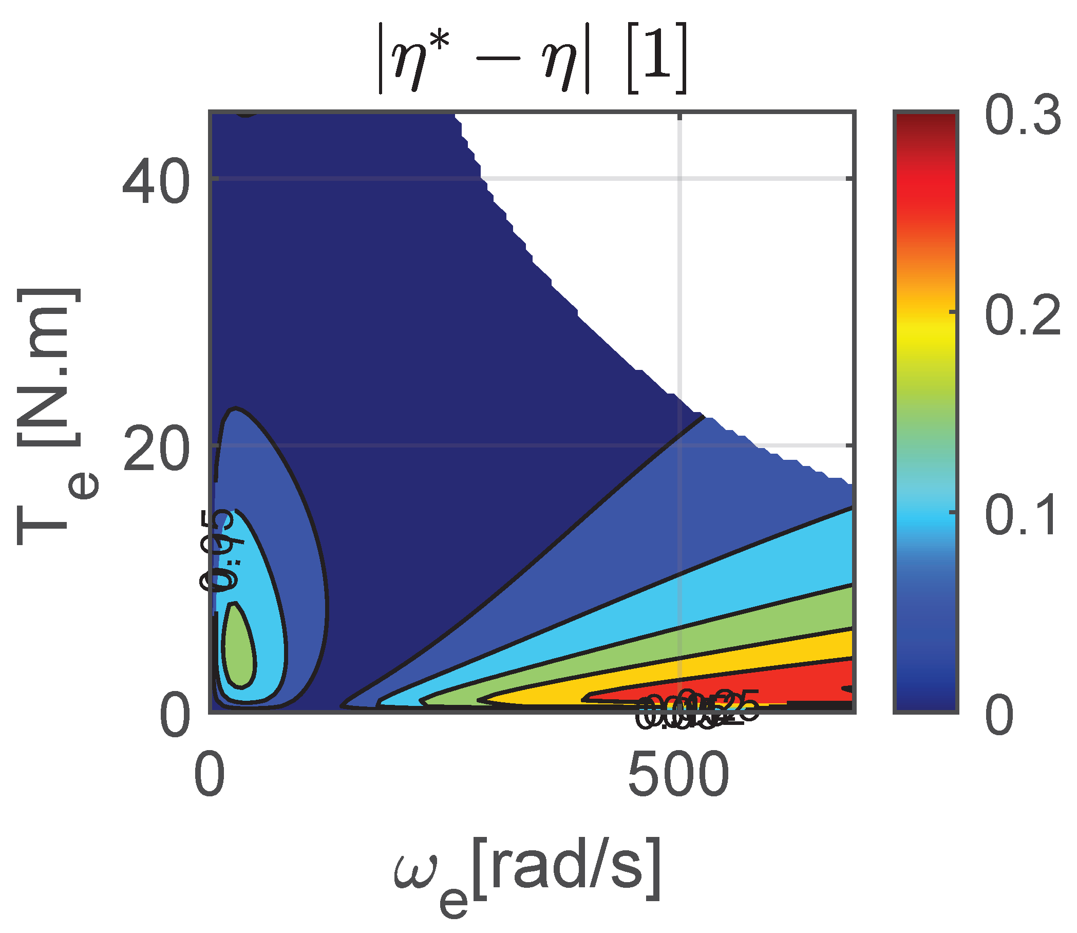
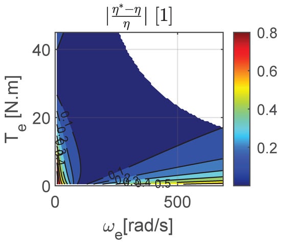
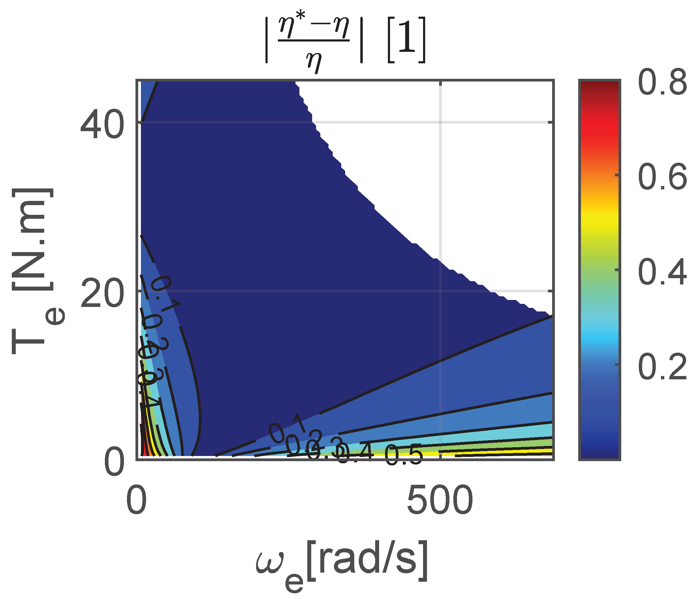
Finally, Figure 22, Figure 23 and Figure 24, respectively, show the efficiencies computed from both measurement sets, along with the absolute and relative errors between the two.
Figure 22.
Overall efficiency.
Figure 23.
Absolute efficiency error.
Figure 24.
Relative efficiency error.
Firstly, it can be observed that the model based on brake measurements predicts the same maximum efficiency value, but over a broader operating region than the prediction coming from torque meter datasets. Finally, the analysis of the absolute and relative error plots confirms the previous observations regarding power losses: the discrepancies between the two models remain small or within acceptable limits at high torque levels.
6. Conclusions
6.1. Summary of Work
In summary, this paper addressed three main topics: the methodology for measuring power losses in electric vehicles, analytical loss modeling, and the use of an on-board torque sensor compared with raw brake-based measurements, after compensating for longitudinal tire slip and test bench friction losses.
Methodology: The first contribution of this paper is the synthesizing and reviewing of the theoretical and practical elements required for experimental implementation, including calibration procedures and the compensation of losses in the tire. It also addresses the modeling aspect by applying the least-squares method and K-fold cross-validation. Appendix A provides a detailed, step-by-step guide to implementing the method proposed in this paper.
Modeling: The second contribution of this paper is the modeling of losses using a two-factor polynomial function, namely torque and rotational speed. The origin and physical justification of first-order losses are reviewed using a second-degree polynomial function, summarized in the form of a 3 × 3 coefficient matrix. This formulation shows that certain terms can be deliberately excluded based on physical considerations. A ‘constrained’ fitting method, enforcing strictly positive loss coefficients, is then implemented and compared with an ‘unconstrained’ approach that may yield negative coefficients. Although the ‘constrained’ method results in a limited loss of accuracy, it offers the advantages of improved coefficient interpretability and the generation of complete efficiency maps, without the need to remove regions where efficiencies may exceed unity—an issue that may occurs with the ‘unconstrained’ method.
On-board torque meter: The third contribution of this paper focuses on the measurement of losses in an electric vehicle using an on-board torque sensor installed on the final drive shaft at the wheel. This experimental approach addresses a gap in the existing literature. A comparative analysis between results obtained from the torque sensor and those derived from brake-based measurements shows that the accuracy of the latter remains acceptable when the motor torque—and consequently the longitudinal tire slip—is sufficiently high. Conversely, when the motor torque or tire slip becomes too low, the resulting errors increase significantly and become clearly unacceptable, thereby making the use of an on-board torque sensor essential.
This analysis was enabled by the use of an experimental vehicle featuring a relatively low maximum motor torque, thereby remaining within the measurement range of a standard, commercially available, ready-to-use torque sensor.
In contrast, typical electric vehicles generally feature motor torque levels that are an order of magnitude higher than those of the vehicle considered in this study. With comparable gear reduction ratios, the resulting driveshaft torque would therefore require a sensor with a much wider measurement range, making the integration of a conventional commercial torque sensor into the transmission shaft particularly challenging. One possible solution to this limitation consists of using a dedicated transmission shaft incorporating an MEMS-based torque measurement system with wireless data transmission [13]. Another approach is to combine measurement methods in a complementary manner, as follows:
- At low motor torque levels, the use of a moderately sized embedded torque sensor ensures sufficient measurement accuracy.
- At high motor torque levels, the torque sensor can be removed, and measurements can instead rely on data obtained from the brake system.
Switching measurement methods during a test campaign inherently entails a risk of systematic error propagation in the resulting loss or efficiency models and maps. To mitigate this risk, it is essential to compare data obtained using both methods within their overlapping operating range and to verify that any observed discrepancies remain within acceptable limits, as performed in the present study.
6.2. Limitations and Future Work
The first limitation of this study lies in the proposed two-variable polynomial function (torque and rotational speed), which does not account for temperature effects. Tire slip behavior, as well as losses in the motor, inverter, and gearbox, are dependent on this parameter. It would therefore be valuable to extend this work by investigating this aspect further, both from an experimental and a modeling perspective.
The second limitation concerns the development of an analytical model applied solely to the motoring region of the powertrain. The regenerative region has not been investigated. This aspect also represents a promising avenue for further extending the present work.
Author Contributions
Conceptualization, P.B., G.C. and P.H.; methodology, P.B.; validation, P.B., G.C. and P.H.; investigation, P.B.; writing—original draft preparation, P.B.; writing—review and editing, G.C. and P.H.; supervision, P.B.; project administration, G.C.; funding acquisition, G.C. All authors have read and agreed to the published version of the manuscript.
Funding
This research received no external funding.
Data Availability Statement
The original contributions presented in this study are included in the article. Further inquiries can be directed to the corresponding author.
Acknowledgments
The authors would like to thank Laurent François and Félix Ramos, technical staff members of the industrial engineering workshop at IUT of Orléans, as well as Pierre Pothin, for their valuable assistance during the experimental campaign.
Conflicts of Interest
The authors declare no conflicts of interest.
Nomenclature
The following abbreviations are used in this manuscript:
| Notation | Units | Designation |
| [1] | Rotational inertia factor | |
| [rad/s] | Front roller angular speed | |
| [rad/s] | Rear roller angular speed | |
| [rad/s] | Electric motor angular speed | |
| [rad/s] | Tire/rim/transmission shaft angular speed | |
| [rad/s] | Ideal angular speed of tire | |
| [1] | Tire longitudinal slip | |
| , | [1] | Overall efficiency from torque meter or brake-based measurement |
| [1] | Tire efficiency | |
| [N] | Motor force developed by tire | |
| [N] | Load cell force | |
| [N] | Eddy current brake force | |
| [N] | Friction force | |
| [N] | Rolling resistance force | |
| [N] | Total resistant force | |
| G | [1] | Total gear reduction ratio |
| J | [kg·m2] | Inertia of vehicle rotating parts |
| [kg·m2] | Inertia of rollers | |
| m | [kg] | Mass of the vehicle |
| [kg] | Equivalent mass simulated by rollers and rotating parts of the vehicle | |
| [kg] | Equivalent mass of the vehicle including rotating parts | |
| [W] | Electric power at battery pack output/Inverter input | |
| [W] | Electric power at inverter output/motor input | |
| [W] | Electric power at electric motor output/speed reducer input | |
| [W] | Electric power at Speed reducer output/tire input | |
| [W] | Electric power at tire output/roller test bench input | |
| [W] | Effective power dissipated at eddy current brake | |
| , | [W] | Overall power loss from torque meter or brake-based measurement |
| , | [W] | Predicted overall power Loss from torque meter or brake based measurement |
| [W] | Inverter power loss | |
| [W] | Electric motor power loss | |
| [W] | Tire power loss due to longitudinal slip | |
| [W] | Roller test bench power loss due to internal friction | |
| [m] | Rollers radius | |
| [m] | Effective loaded radius of tire in free-wheel condition | |
| R | [m] | Effective loaded radius of tire under torque |
| , | [N·m] | Torque at drive shaft from torque meter or brake-based measurement |
| , | [N·m] | Torque at electric motor shaft from torque meter or brake based measurement |
| [m/s] | Tangential speed on rollers/Vehicle speed |
Appendix A. Step-by-Step Guide to Implementing the Proposed Method
Step 1: Design the modified drive shaft to integrate the most suitable torque meter.
Step 2: Open the electrical circuit upstream of the inverter to insert a current measurement device (shunt for example).
Step 3: Measure the free-rolling radius of the tire, , on the roller bench using the roller encoders and (23). For example, perform ten full manual revolutions of the wheel while recording the rollers’ angular displacement.
Step 4: Calculate the vehicle’s equivalent mass on the test bench. (Refer to Section 3.3.1).
Step 5: Perform several coast-down tests in neutral gear to determine the resistive force . (Refer to Section 3.3.2 and (4)).
Step 6: Calibrate the eddy current brake load cell. Furthermore, calibrate the current measurement system, whether using the shunt resistor and/or data retrieved from Battery Management System CAN messages. (Refer to Section 3.4).
Step 7: Conduct the experimental campaign using the torque meter, covering the widest possible range of steady-state operating points. Each point should be repeated, for example, five times. Record the following measurements: , , , , , and or .
Step 8: If necessary, remove the torque meter equipped shaft and complete the experimental dataset by measuring: , , , , and or .
Step 9: Compute the electrical input power at the inverter Equation (17) or (18), then the mechanical power at the wheel using Equation (2), and finally the motor torque using Equation (31).
Step 10: At each operating point, calculate the total resistant force using (16), then deduce the traction force (according to (4) in steady state condition) and the output power at the wheel using (26). Compute the tire’s longitudinal slip using (22), and from this, determine from (25) the corrected input power and finally the estimated torques and .
Step 11: Calculate the total power losses using (1) as well as . Compute the efficiencies et .
Step 12: Filter the measurement data by excluding clearly erroneous points (e.g., , , etc.). For each operating point, retain the median value of overall losses from the remaining valid samples.
Step 13: Plot and verify that the tire operates within its linear region. Exclude any data points that fall outside this range.
Step 14: Plot the following graphs:
- .
- Absolute error: .
- Relative error: .
Check for the presence of any systematic bias. If a significant bias is observed, first verify the tire radius , the friction loss calibration of the test bench and the calibration of the brake load cell.
Step 15: Merge the two datasets (torque-meter- and brake-based) to produce a single measurement set covering the widest possible operating range.
Step 16: Perform an unconstrained least-squares fit using all nine coefficients . Check overfitting or underfitting using a K-fold cross validation process. Compute the RMSE and mean value of residuals of this ‘optimal’ but non-physical model. Refer to Section 3.8.
Step 17: Carry out a ‘constrained’ iterative fit, starting with the six physically meaningful coefficients. Ensure that the final set of coefficients should be strictly positive or zero. Check overfitting or underfitting using a K-fold cross validation process. Compute the RMSE and mean value of residuals of the ‘constrained’ fit and compare it to that of the ‘unconstrained’ fit to assess its acceptability.
Step 18: Generate loss and efficiency maps based on the identified model.
Appendix B. Technical Information
Table A1.
Renault TWIZY 80 technical specifications.
Table A2.
Torque Sensor specifications from https://www.burster.com/fileadmin/user_upload/redaktion/Documents/Products/Data-Sheets/Section_8/8661_EN.pdf (accessed on 8 Febuary 2026).
Table A3.
Roller test bench technical specifications.
References
- IEA. Global EV Outlook 2025. Available online: https://www.iea.org (accessed on 15 February 2026).
- Kumar, S.; Singh, V.; Goel, R. Strategic Forecasting for Electric Vehicle Sales: A Cutting Edge Holistic Model Leveraging Key Factors and Machine Learning Technique. Transp. Dev. Econ. 2024, 10, 23. [Google Scholar] [CrossRef] [Scilit]
- Torinsson, J.; Jonasson, M.; Yang, D.; Jacobson, B. Energy reduction by power loss minimisation through wheel torque allocation in electric vehicles: A simulation-based approach. Veh. Syst. Dyn. 2022, 60, 1488–1511. [Google Scholar] [CrossRef] [Scilit]
- Janiaud, N.; Vallet, F.X.; Petit, M.; Sandou, G. Electric vehicle powertrain simulation to optimize battery and vehicle performances. In Proceedings of the 2010 IEEE Vehicle Power and Propulsion Conference, Lille, France, 1–3 September 2010; pp. 1–5. [Google Scholar] [CrossRef] [Scilit]
- Roshandel, E.; Mahmoudi, A.; Kahourzade, S.; Yazdani, A.; Shafiullah, G. Losses in Efficiency Maps of Electric Vehicles: An Overview. Energies 2021, 14, 7805. [Google Scholar] [CrossRef] [Scilit]
- Sun, B.; Gao, S.; Ma, C.; Li, J. System power loss optimization of electric vehicle driven by front and rear induction motors. Int. J. Automot. Technol. 2018, 19, 121–134. [Google Scholar] [CrossRef] [Scilit]
- Valladolid, J.D.; Albarado, R.; Mallahuari, D.; Patiño, D. Experimental Performance Evaluation of Electric Vehicles (EV) Based on Analysis of Power and Torque Losses. In Proceedings of the 2020 IEEE International Conference on Industrial Technology (ICIT), Buenos Aires, Argentina, 26–28 February 2020; IEEE: New York, NY, USA, 2020; pp. 933–938. [Google Scholar] [CrossRef] [Scilit]
- Nguyen, Q.K.; Roth-Stielow, J. Analysis and Modelling of the Losses for the Electrical Drive System of an Electric Vehicle. In Proceedings of the 2014 IEEE Vehicle Power and Propulsion Conference (VPPC), Coimbra, Portugal, 27–30 October 2014; IEEE: New York, NY, USA, 2014; pp. 1–6. [Google Scholar] [CrossRef] [Scilit]
- Hengst, J.; Werra, M.; Küçükay, F. Evaluation of Transmission Losses of Various Battery Electric Vehicles. Automot. Innov. 2022, 5, 388–399. [Google Scholar] [CrossRef] [Scilit]
- De Santis, M.; Agnelli, S.; Patanè, F.; Giannini, O.; Bella, G. Experimental Study for the Assessment of the Measurement Uncertainty Associated with Electric Powertrain Efficiency Using the Back-to-Back Direct Method. Energies 2018, 11, 3536. [Google Scholar] [CrossRef] [Scilit]
- Rosenberger, N.; Lienkamp, M. Vehicle Parameter and Electric Powertrain Efficiency Analysis Using Real-Driving Data. Int. J. Electr. Electron. Eng. Telecommun. 2024, 13, 494. [Google Scholar] [CrossRef] [Scilit]
- Silva, M.; Goncalves, A.P.; Marques, J.; Sousa, J.; Nunes, U. Modelling an Electric Vehicle Powertrain on Bench. In Proceedings of the 2014 IEEE Vehicle Power and Propulsion Conference (VPPC), Coimbra, Portugal, 27–30 October 2014; IEEE: New York, NY, USA, 2014; pp. 1–6. [Google Scholar] [CrossRef] [Scilit]
- Folta, Z.; Hrudičková, M. Experience with Torque Measurement on Rotating Shaft. Trans. Electr. Eng. 2013, 2, 77–83. [Google Scholar]
- Tawadros, P.; Awadallah, M.; Walker, P.; Zhang, N. Using a low-cost bluetooth torque sensor for vehicle jerk and transient torque measurement. Proc. Inst. Mech. Eng. Part D J. Automob. Eng. 2020, 234, 423–437. [Google Scholar] [CrossRef] [Scilit]
- La fabrique des mobilités. Twizy Open Source—P.O.M. 2020. Available online: https://wiki.lafabriquedesmobilites.fr/wiki/Twizy_Open_Source_-_P.O.M. (accessed on 15 February 2026).
- Eduscol. Modélisation Multiphysique de la Renault Twizy. 2022. Available online: https://eduscol.education.fr/sti/ressources_techniques/modelisation-multiphysique-de-la-renault-twizy (accessed on 15 February 2026).
- openVehicles. Open-Vehicle-Monitoring-System. 2017. Available online: https://github.com/openvehicles/Open-Vehicle-Monitoring-System/blob/master/docs/Renault-Twizy/CANBUS-Objektverzeichnis.ods (accessed on 15 February 2026).
- Cavallo, S. Modeling of a Roller Test Bench for Car Homologation. Master’s Thesis, Politecnico di Torino, Turin, Italy, 2021. [Google Scholar]
- Gilormini, T. Développement d’une MéThodologie de Tests de VéHicules Automobiles Combinant ModèLes NuméRiques et Banc D’Essais Moteur (Approche HIL). Ph.D. Thesis, École Centrale de Nantes, Nantes, France, 2022. [Google Scholar]
- Ehsani, M.; Gao, Y.; Emadi, A. Modern Electric, Hybrid Electric, and Fuel Cell Vehicles Fundamentals, Theory, and Design, 2nd ed.; CRC Press: Boca Raton, FL, USA, 2009; Chapter 2. [Google Scholar] [CrossRef] [Scilit]
- Fajri, P.; Ahmadi, R.; Ferdowsi, M. Equivalent vehicle rotational inertia used for electric vehicle test bench dynamic studies. In Proceedings of the IECON 2012—38th Annual Conference on IEEE Industrial Electronics Society, Montreal, QC, Canada, 25–28 October 2012; IEEE: New York, NY, USA, 2012; pp. 4115–4120. [Google Scholar] [CrossRef] [Scilit]
- Pacejka, H. Tyre and Vehicle Dynamics; Elsevier Science Publication: Amsterdam, The Netherlands, 2006. [Google Scholar]
- Sina, N.; Esfahanian, V.; Hairi Yazdi, M.; Azadi, S. Introducing the Modified Tire Power Loss and Resistant Force Regarding Longitudinal Slip. SAE Int. J. Passeng. Cars-Mech. Syst. 2018, 11, 167–176. [Google Scholar] [CrossRef] [Scilit]
- Singh, K.; Taheri, S. Estimation of tire–road friction coefficient and its application in chassis control systems. Syst. Sci. Control Eng. 2014, 3, 39–61. [Google Scholar] [CrossRef] [Scilit]
- Mahmoudi, A.; Soong, W.L.; Pellegrino , G.; Armando, E. Efficiency maps of electrical machines. In Proceedings of the IEEE Energy Conversion Congress and Exposition (ECCE), Montreal, QC, Canada, 20–24 September 2015; IEEE: New York, NY, USA, 2015. [Google Scholar] [CrossRef] [Scilit]
- Larminie, J.; Lowry, J. Electric Vehicle Technology Explained; John Wiley and Sons: Hoboken, NJ, USA, 2003. [Google Scholar]
- Sarrazin, B. Optimisation d’une Chaîne de Traction Pour Véhicule Électrique. Ph.D. Thesis, Université de Grenoble, Grenoble, France, 2012. [Google Scholar]
- Monaco, G.; Fedullo, A. Teaching Least Squares in Matrix Notation. Ratio Math. 2017, 32, 63–75. [Google Scholar] [CrossRef] [Scilit]
- Kohavi, R. A Study of Cross-Validation and Bootstrap for Accuracy Estimation and Model Selection. In Proceedings of the Fourteenth International Joint Conference on Artificial Intelligence (IJCAI), Montreal, QC, Canada, 20–25 August 1995; pp. 1137–1143. [Google Scholar]
- Cabrera, J.A.; Castillo, J.J.; Pérez, J.; Velasco, J.M.; Guerra, A.J.; Hernández, P. A Procedure for Determining Tire-Road Friction Characteristics Using a Modification of the Magic Formula Based on Experimental Results. Sensors 2018, 18, 896. [Google Scholar] [CrossRef] [Scilit] [PubMed]
- Biffi, A.; Gobbi, M.; Mastinu, G. Tyre rolling resistance and tyre rolling loss: A theoretical and experimental study based on a new trailer. Meccanica 2025, 60, 2561–2585. [Google Scholar] [CrossRef] [Scilit]
- Santiago, J.D. Electrical Motor Drivelines in Commercial All-Electric Vehicles: A Review. IEEE Trans. Veh. Technol. 2012, 61, 484. [Google Scholar] [CrossRef] [Scilit]
- Lukic, S.; Emado, A. Modeling of electric machines for automotive applications using efficiency maps. In Proceedings of the Proceedings: Electrical Insulation Conference and Electrical Manufacturing and Coil Winding Technology Conference (Cat. No. 03CH37480), Indianapolis, IN, USA, 25–25 September 2003; pp. 543–550. [Google Scholar] [CrossRef] [Scilit]

Disclaimer/Publisher’s Note: The statements, opinions and data contained in all publications are solely those of the individual author(s) and contributor(s) and not of MDPI and/or the editor(s). MDPI and/or the editor(s) disclaim responsibility for any injury to people or property resulting from any ideas, methods, instructions or products referred to in the content. |
© 2026 by the authors. Licensee MDPI, Basel, Switzerland. This article is an open access article distributed under the terms and conditions of the Creative Commons Attribution (CC BY) license.