


Abstract
For addressing the challenge that cross-interconnection of metal sheaths in long-distance high-voltage cables complicates the monitoring of cable insulation faults, it is proposed a fault diagnosis scheme based on resistive current, dielectric loss factor, and sheath current. The voltage and current signals at both ends of the cable are collected, as well as the current signals at the outlet of the grounding box and the transposition box. By establishing an equivalent model of the cross-connected cable, the calculation method for fault diagnosis is derived, and an implementation scheme for fault diagnosis is provided. The insulation monitoring method proposed in this paper is simulated and verified using MATLAB/Simulink software, with simulations conducted to investigate four typical faults: cable insulation fault, sheath open-circuit fault, transposition box immersion short-circuit fault, and cable intermediate-joint breakdown fault. The circuit model of the cross-connected unit is established in the laboratory to verify the method proposed in this paper. The results show that the simulation results are consistent with the test results, and the fault types can be correctly reflected, which verifies the correctness and effectiveness of the insulation monitoring method.
1. Introduction
The rapid development of society and the economy has led to a significant increase in electricity demand across various industries. The scale of the transmission and distribution grid is also undergoing rapid expansion, with development accelerating year after year. Power cables, as the key equipment for transmission and distribution, are used in large quantities in the transmission lines of the power system, particularly in the field of extra-high-voltage power transmission [1]. Single-core high-voltage cables are prone to the generation of significant induced voltages due to the operation of their metal sheath. The magnitude of this induced voltage is directly proportional to the length and value of the cable. The presence of induced voltages in long-distance high-voltage cables has the potential to cause damage to the sheath insulation, which could ultimately result in the destruction of the main insulation [2,3]. Consequently, unbalanced currents in the sheath can restrict the cable’s current-carrying capacity [4,5]. To address this issue, metal sheath cross-interconnections are typically employed to diminish circulating currents within the sheath and minimize induced voltages [6,7]. However, the utilization of such cable configurations renders cable insulation monitoring and fault diagnosis challenging.
Presently, the cable insulation online monitoring methods most utilized in domestic and international contexts encompass the dielectric loss factor method, resistive current method, partial discharge monitoring method, and other analogous techniques [8]. Most cable insulation online monitoring methods are primarily utilized for short-distance single-ended or double-ended grounded power cables. However, for high-voltage long-distance cable insulation monitoring with a cross-interconnection structure, numerous methods are no longer applicable, and there is a paucity of research outcomes in this domain. Accordingly, the implementation of real-time insulation condition monitoring for long-distance high-voltage cables is significant for ensuring the reliable operation of power systems, as it enables the prompt identification of the type and location of any fault that may occur.
Zhang Hailong et al. [9] from Wuhan University integrated the robust pattern recognition capabilities of neural networks with the intrinsic properties of cross-interconnected cables, thereby proposing a novel approach for real-time monitoring of cable insulation conditions. Yang Longtao et al. [10] constructed a distribution parameter model of cross-interconnected power cables, analyzed the primary insulation faults that cables are susceptible to through simulation, and made an initial determination of the fault location. Yuan Yanling et al. [11] put forth a set of criteria for discerning cable faults and their locations through the modeling of three-phase cross-interconnected cables and the analysis of sheath current values under diverse cable insulation faults. Zhou Wenjun et al. [12] employed an equivalent model of a cross-interconnection cable system to separate the leakage current of any small section of cable within the system. They then proposed a method of analyzing the relative change in phase-to-phase dielectric loss. However, the aging criterion provided is complex and does not fully account for the specific type of fault. Yang Jing et al. [13] considered the effect of induced voltage in the sheath and proposed a method of cable fault diagnosis using the measured current at the outlet end of the cross-bonding link box. The method was verified through simulation, although the main insulation faults of the cable were not addressed. Zhu Bo et al. [14] from the Harbin Institute of Technology put forth a methodology for fault diagnosis, which entails calculating resistive current and sheath loop current based on measured currents at the outlet end of the grounding box and the cross-bonding link box. However, the criterion for insulation faults is rather intricate. Lai Shengjie et al. [15] established a double-π centralized parameter model for cables and proposed a method for calculating the metallic sheath ring current. This method involves neglecting the resistive current and considering the capacitive leakage current and the sheath-induced current. Lulu Li et al. [16] employed the transient response of currents on grounding and cross-interconnection lines in the context of system power disturbances, with the objective of discerning the overall aging state of cables. This was achieved through the calculation of insulation conductance spectra. However, the proposed scheme of installing current transformers on each section of cross-interconnection lines proved challenging to implement. Du Boxue et al. [17] developed a mathematical model for calculating grounding currents in cross-interconnection structures of single-core cables. They also proposed a fault diagnosis method based on sheath currents, but their model did not account for the influence of leakage currents. Zhang Leiqi et al. [18] conducted an experimental investigation into the attenuation characteristics of local discharge signals propagating along cables and the coupling effect of cable conductor layers and shielding layers. They employed high-frequency current sensors to detect partial discharge waveforms at various cross-interconnection grounding points. However, the local discharge waveforms are complex and variable, and the signals are weak and difficult to distinguish.
This paper proposes the use of resistive current, dielectric loss factor, and sheath loop current as characteristic parameters for characterizing the insulation condition of long-distance cross-interconnection cables. The type of faults and fault locations are determined by monitoring the changes in these characteristic parameters when faults occur. The results are verified through simulation, and the proposed insulation monitoring method is shown to be effective. The practical application will enhance the reliability and stability of the power supply.
2. Modeling Cross-Interconnect Cable Circuits
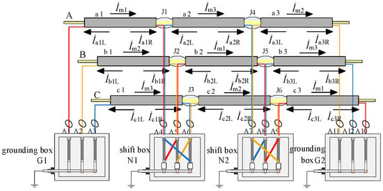
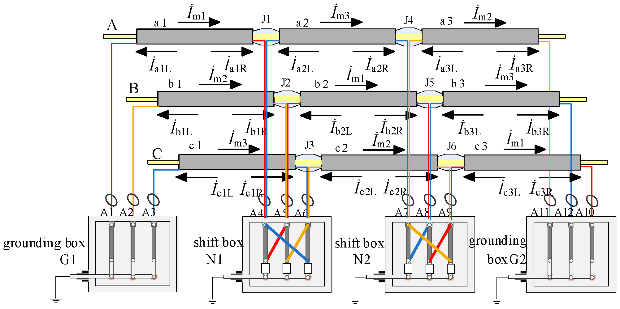
Long-distance high-voltage cables are composed of several cross-interconnection units, one of which is illustrated schematically in Figure 1.
Figure 1.
The schematic diagram of the crossed interconnection.
Each standard cross-interconnection unit comprises the division of each phase of the cable into three segments on average. Following cross-interconnection through the coaxial cable via the cross-bonding link box, the metal sheath of each small segment of the cable is grounded. Accordingly, the induced voltage can be theoretically eliminated. However, in actual operation, in accordance with the relevant specifications, the induced voltage on the metal sheath of each section of the cable is not more than 50 V [19]. The parameters used in the figure are as follows: conductor cross-sectional area: 800 mm2, cable outer diameter: 100 mm, conductor diameter: 34 mm, insulation thickness: 16 mm, outer shielding thickness: 1.0 mm, inner shielding thickness: 1.2 mm, sheath thickness: 4.5 mm. The equivalent parameters of single-segment cable are as follows: the length of each segment is 0.4 km, the equivalent resistance of the main insulation is 179 (R/MΩ), the equivalent capacitance of the main insulation is 78.8 (C/nF), the equivalent resistance of the cable core is 6.56 (R/mΩ), and the equivalent inductance of the cable core is 42.76 (L/μH).
The presence of an induced voltage results in the generation of a sheath loop current within the sheath circuit. This current flows from the initial end to the end of the circuit, as illustrated below: İm1, İm2, İm3. The sheath loop current and the leakage current through the main insulation collectively constitute the sheath loop current. The condition of the insulation in the cable can be ascertained by examining the fluctuations in the sheath loop current.
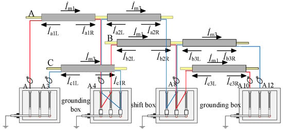
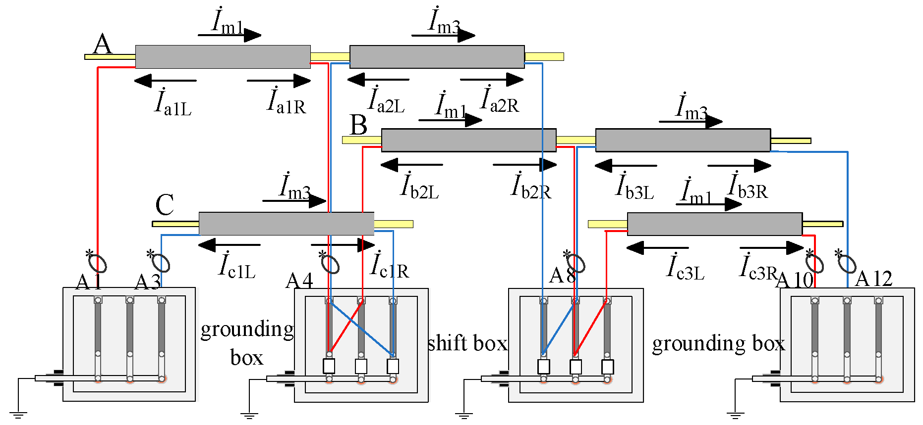
The current transformers are situated at the outgoing wires of the changeover and grounding boxes, as illustrated in Figure 2. As illustrated in the figure, the current transformers situated at the external outlets of grounding boxes G1, G2 and cross-bonding link boxes N1, N2 are designated as A1–A12. In view of the particularity of the cross-connected structure of long-distance high-voltage cable, in order to accurately obtain the key monitoring parameters such as sheath loop current and leakage current active component, this study adopts the configuration scheme of 12 current transformers (CTs) and needs to select high-precision metering level CT to meet the weak signal measurement requirements. From the perspective of cost composition, this study selects 0.2S-level high-precision measurement CT, and its single market price is about 1.5 times that of conventional protection CT; however, through the project batch procurement mode, combined with the technical cooperation agreement with the equipment supplier, the cost can be significantly reduced. The average loss of total sensor investment relative to the power outage caused by a single insulation fault is negligible. From the perspective of return on investment, the payback period of sensor networks is about 1.2 years, which has significant economic feasibility. The measured sheath currents are designated as İA1–İA12, the outlets of cross-bonding link boxes N1 and N2 are equipped with coaxial cables, and the currents measured by the current transformers installed thereon represent the vector sums of currents in the metal sheaths of small sections of the cables of the same phase. In this context, the leftward component of the leakage current of each cable segment in the metal sheath is designated as İaiL, İbiL, İciL (i = 1, 2, 3), while the rightward component is designated as İaiR, İbiR, İciR (i = 1, 2, 3). By the application of Kirchhoff’s first law, the following relationships are established:
Figure 2.
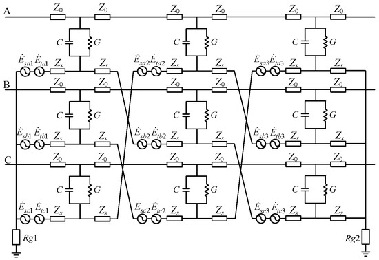
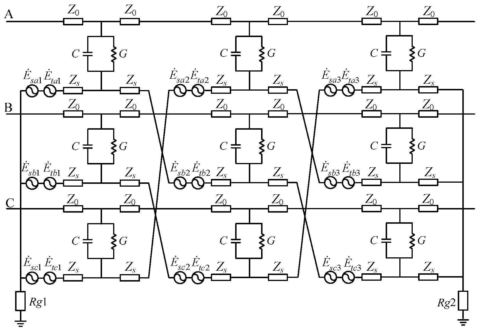
Equivalent circuit of a unit of cross-linked three-phase power cable.
The leakage currents of the cables in each sub-section of phases A, B, and C are represented by the variables İai (i = 1, 2, 3), İbi (i = 1, 2, 3), and İci (i = 1, 2, 3), respectively.
By establishing the above equivalent circuit model, it provides a theoretical basis for the derivation of subsequent monitoring parameters. Based on this model, the calculation methods of active component, dielectric loss factor, and sheath loop current will be studied in the following.
3. Calculation Method
3.1. Cross-Interconnection Unit Sheath Loop Current Calculation
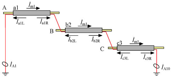
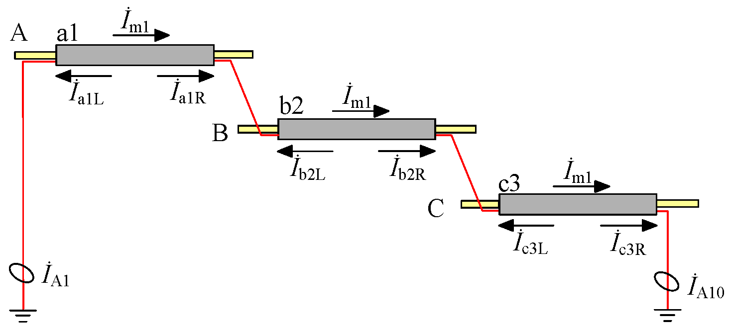
To illustrate, the current distribution for the sheath circuit a1-b2-c3 is depicted in Figure 3 and Figure 4. The current transformers situated at the extremities of the sheath circuit, designated as A1 and A10, respectively, have been observed to yield measured current values of İA1 and İA10. To facilitate the calculations, the direction of the current in the sheath circuit is specified to be positive to the left, and there are:
Figure 3.
Sheath circuit a1-b2-c3 current distribution.
Figure 4.
The current distribution of two adjacent branches in the transposition box.
Similarly, the expressions for the measured currents (İA2, İA3, İA11, and İA12) of the other two guard circuit current transformers can be derived as follows:
Subsequently, the currents in the three sheath circuits can be expressed as follows:
Accordingly, the value of the circuit current of each sheath can be calculated using the methodology illustrated in Equation (5), with the values of the two current transformers as inputs. Furthermore, the cable insulation condition can be characterized in accordance with its change rule.
3.2. Cross-Interconnection Unit Resistive Current Separation
The existing configuration of the two adjacent branches within the cross-bonding link box is illustrated in Figure 4.
In the case of the current transformer A4, the current measured by it can be understood as the vector sum of the currents in the metal sheath of the small sections of the cable of the same phase. In other words, it can be seen as the vector sum of the currents of the circuits a1-b2-c3 and the circuits c1-a2-b3. Additionally, it can be considered as the current vector of the circuit İA4.
In a similar manner, the measured values of current transformers A5–A9 can be expressed as follows:
The expression can be derived by organizing the fundamental Equations (2)–(4) in a systematic manner:
Upon substituting the expressions for İm1 and İm3 in Equation (8) into Equation (6) and organizing them, the following expressions are obtained:
Similarly, upon substituting the corresponding expression in Equation (8) into Equation (7) and organizing it, the following result is obtained:
By aggregating the measured currents from each current transformer, a comprehensive overview can be obtained:
Similarly, it can be demonstrated that:
The three equations in Equations (11) and (12) are summed separately to obtain the result:
The addition of the three equations from Equation (5) results in the following expression:
The calculations presented in Equations (9), (10), (13) and (14) can be organized systematically to arrive at the desired result:
The leakage currents of each phase of the cross-interconnection unit can be calculated separately from Equation (15). Furthermore, the current transformers utilized in the algorithm for the calculation of each phase are limited to four, which contributes to the algorithm’s overall simplicity and practicality.
The resistive current and leakage current of the cross-interconnection unit are separated, and the reference voltage is selected as the vector sum of the voltages at the first and last terminals of each phase of the long-distance cable [20], divided by two. The equivalent impedance (Z) of the main insulation of the A-phase cable is then calculated:
Additionally, the definition of impedance indicates that the impedance of the primary insulation of the cable is equivalent to the equivalent resistance, resulting in an equivalent impedance value:
In Equation (17), R represents the equivalent resistance of the primary insulation of the cable, C denotes the equivalent capacitance between the cable conductor and the metallic sheath, and ω signifies the angular velocity of the system during operational conditions. The expression for the resistive current in phase A of the cross-interconnection unit is derived from the combination of Equations (16) and (17):
Similarly, the sum of the resistive currents flowing through the cable insulation of phases B and C of the cross-interconnection unit can be obtained as follows:
Concurrently, the dielectric loss factor of the phase A insulation of the cross-interconnection unit can be determined to be:
The derivation of the aforementioned formula allows for the calculation of the resistive current and dielectric loss factor of each phase of the cross-interconnection unit. As a monitoring parameter, the resistive current and dielectric loss factor can be used to assess the insulation condition of the cable, given their variable value. The calculation method of monitoring parameters derived in this section provides the core algorithm support for fault diagnosis. The next section will build a simulation model through MATLAB/Simulink to verify the feasibility of the method.
4. Modeling Three-Phase Cable Simulation
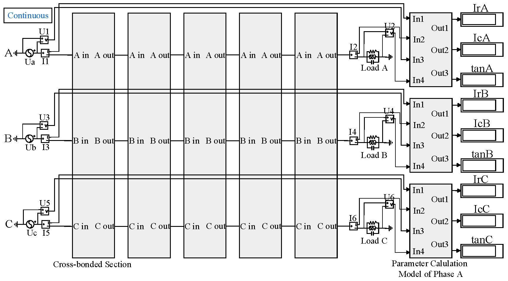
A simulation model of a three-phase cable insulation fault is constructed using the MATLAB/Simulink tool. The simulation model is used to simulate different fault types by changing the parameters of the equivalent circuit. The change rule of the insulation monitoring parameters is also recorded. The total length of each phase of the cable is set to 12 km, with one cross-interconnection unit measuring 1.2 km and each cable subsection measuring 0.4 km. The long-distance single-phase cable simulation model is shown in Figure 5.
Figure 5.
Long-distance single-phase cable insulation fault simulation model.
Each two cross-interconnection units are encapsulated in a module, and the algorithmic part of the monitoring parameters is encapsulated in a module. The three-phase voltage sources are denoted by Ua, Ub, and Uc, and the loads are denoted by RLC shunt modules. The voltage transformers (U1–U6) are utilized to measure the voltage at the initial and final terminals of the three phases of cable A, B, and C, respectively. Similarly, the current transformers (I1–I6) are employed to measure the core current at the aforementioned terminals. The simulation model of the cross-interconnection unit is illustrated in Figure 6.
Figure 6.
Insulation monitoring simulation model of cable cross-interconnection unit.
The voltage level established in the simulation model is 110 kV; the frequency is that of an industrial power system, 50 Hz; and the cable is laid in an equilateral triangle configuration by default. The cable size parameters are presented in Table 1, in accordance with the national standard GB/T11017.2-2014.
Table 1.
Parameters of 110 kV XLPE cable.
In accordance with the cable parameters illustrated in Table 1, the electrical parameters of the cable are determined. The unit equivalent resistance of the core is R0 = 3.28 × 10⁻⁵ Ω/m, the unit equivalent inductance is L0 = 2.138 × 10⁻⁷ H/m, the unit equivalent conductance of the main insulation is G0 = 1.397 × 10⁻¹¹ S/m, and the unit equivalent capacitance is C0 = 1.971 × 10⁻¹⁰ F/m. Based on these parameters, the calculations yield the electrical parameters of each cable sub-section of the simulation model, as presented in Table 2.
Table 2.
Electrical parameters of each cable segment.
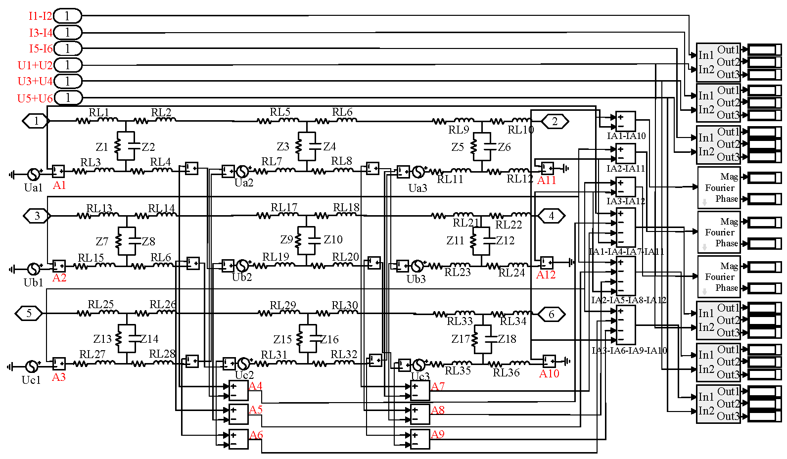
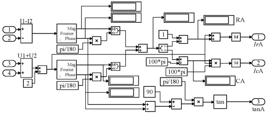
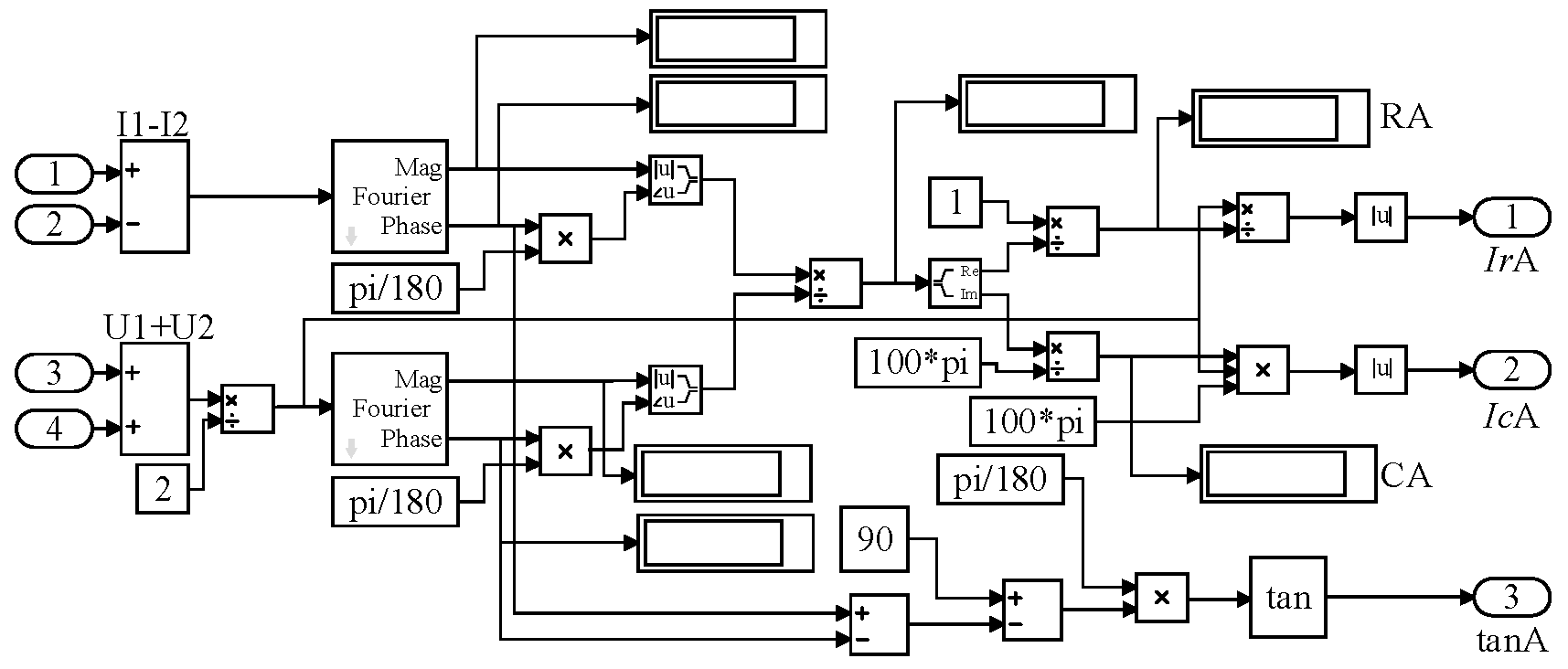
To illustrate, the algorithmic component of the simulation model for monitoring the parameters in phase A is depicted in Figure 7. In this figure, the Fourier module is employed to calculate the modulus and phase angle of the reference voltage and leakage current signals. The result of the simulation calculation of the dielectric loss factor is tanA, the result of the simulation calculation of the resistive current is IrA, and the result of the simulation calculation of the capacitive current is IcA.
Figure 7.
A-phase cable overall resistive current and dielectric loss factor simulation cross-bonding link box model.
As illustrated in Figure 7, the insulation monitoring scheme incorporates the addition of current transformers A1~A12 to the simulation model. This allows for the monitoring of currents at the outgoing terminals of the grounding box and the transposition box, respectively. Utilize this simulation model to simulate the cross-interconnection unit under normal conditions for each protection layer circuit current, each phase dielectric loss factor, and each phase resistive current. In order to accurately measure the active component of the weak leakage current and the current of the sheath circuit at the outlet end of the grounding box and the transposition box, a 0.2S high-precision metering current transformer is selected in this study, and its core technical parameters are shown in Table 3. This type of CT has low phase error, high amplitude accuracy, and wide frequency adaptability, which can meet the stringent requirements of phasor calculation for measurement accuracy in this study. The simulation results are presented in Table 4 and Table 5.
Table 3.
Core technical parameters for the 0.2S class current transformer.
Table 4.
The theoretical and simulation values of the resistive and sheath current of each branch.
Table 5.
Theoretical value and simulation value of dielectric loss factors of each phase.
As evidenced in Table 4 and Table 5, the discrepancy between the simulated and calculated values and the theoretical values of the resistive current of each branch, the dielectric loss factor of each phase, and the sheath circuit current is no greater than 0.5%. This suggests that it is feasible to utilize the resistive current, dielectric loss factor, and sheath circuit current, which have been calculated from the measured values of the current transformer, as monitoring parameters for insulation monitoring.
Based on the above simulation model, the following will simulate a variety of typical fault scenarios, analyze the variation of monitoring parameters, and verify the fault diagnosis ability of the method.
5. Fault Simulation
5.1. Cable Insulation Fault Simulation
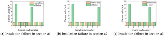
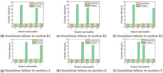
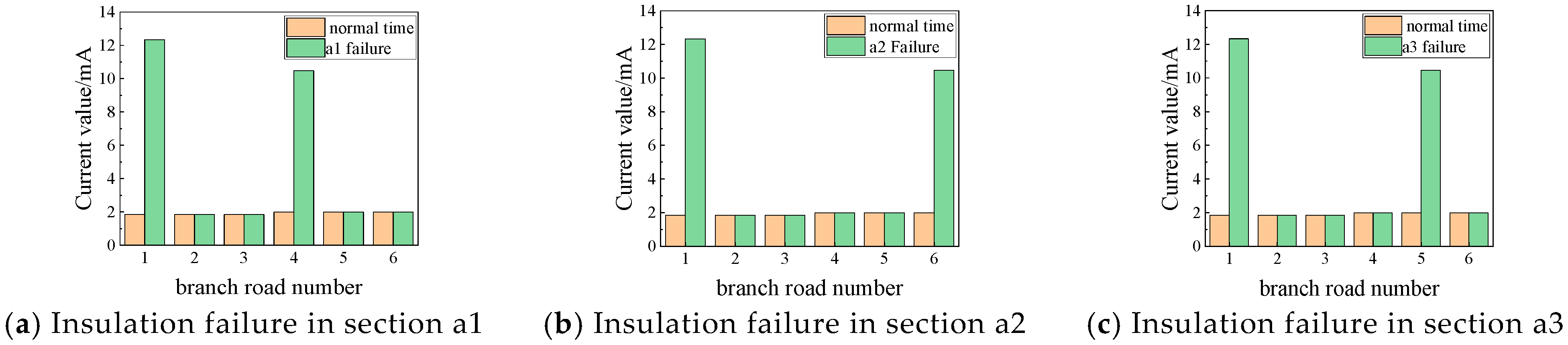
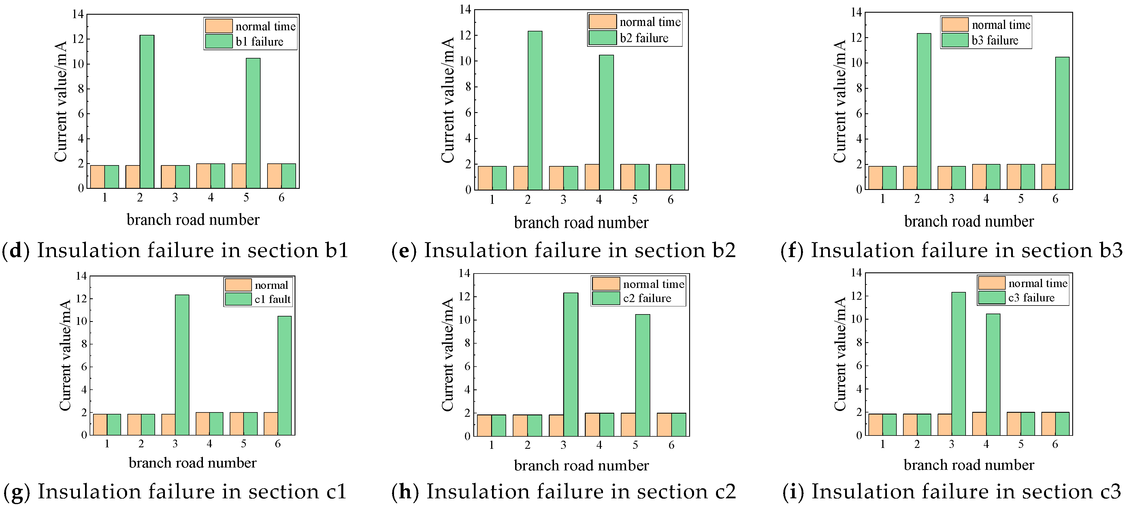
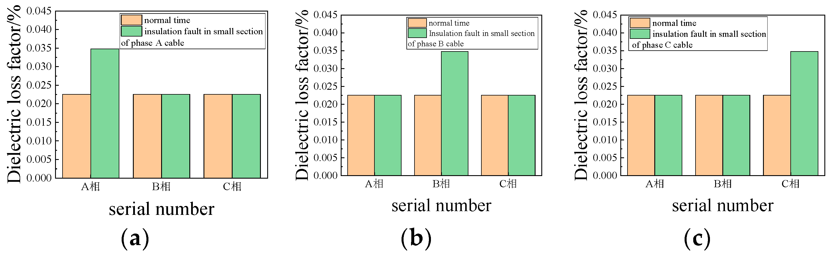
In order to simulate a cable insulation fault, the insulation resistance and capacitance of a small section of the cable were set to 1 MΩ and 120 nF, respectively. The resulting simulation results are presented in Figure 8 and Figure 9. The branch sequence numbers in the figure represent the resistive currents of phases A, B, and C, as well as the currents of the sheath circuits a1-b2-c3, b1-c2-a3, and c1-a2-b3, respectively.
Figure 8.
Resistive current and sheath circuit current of any small insulation fault.
Figure 9.
The dielectric loss factor of any small section of insulation fault. (a) Insulation fault in small section of phase A cable; (b) Insulation fault in small section of phase B cable; (c) Insulation fault in small section of phase C cable.
As illustrated in Figure 8 and Figure 9, in the cross-interconnection unit, the failure of a section of cable insulation results in a notable increase in both the resistive current and sheath current of the relevant branch in which it is located. Additionally, the dielectric loss factor of the phase in which the failure occurs also exhibits a considerable rise. For instance, monitoring of branch a1-a2-a3 reveals a notable increase in resistive current, accompanied by a corresponding rise in the A phase of the dielectric loss factor. Concurrently, the branch a1-b2-c3 sheath circuit current exhibits a substantial surge. These observations collectively indicate that the cross-interconnection unit of the cable failure pertains to the A-phase of the a1 section. The same methodology is applicable to the analysis of other insulation segment faults.
5.2. Metal Sheath Open-Circuit Faults
Metal sheath open-circuit faults are further divided into the grounding box G1, G2 and transposition box N1, N2 within the sheath open-circuit faults, open-circuit faults occurring in different locations based on different judgments.
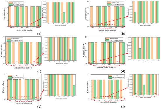
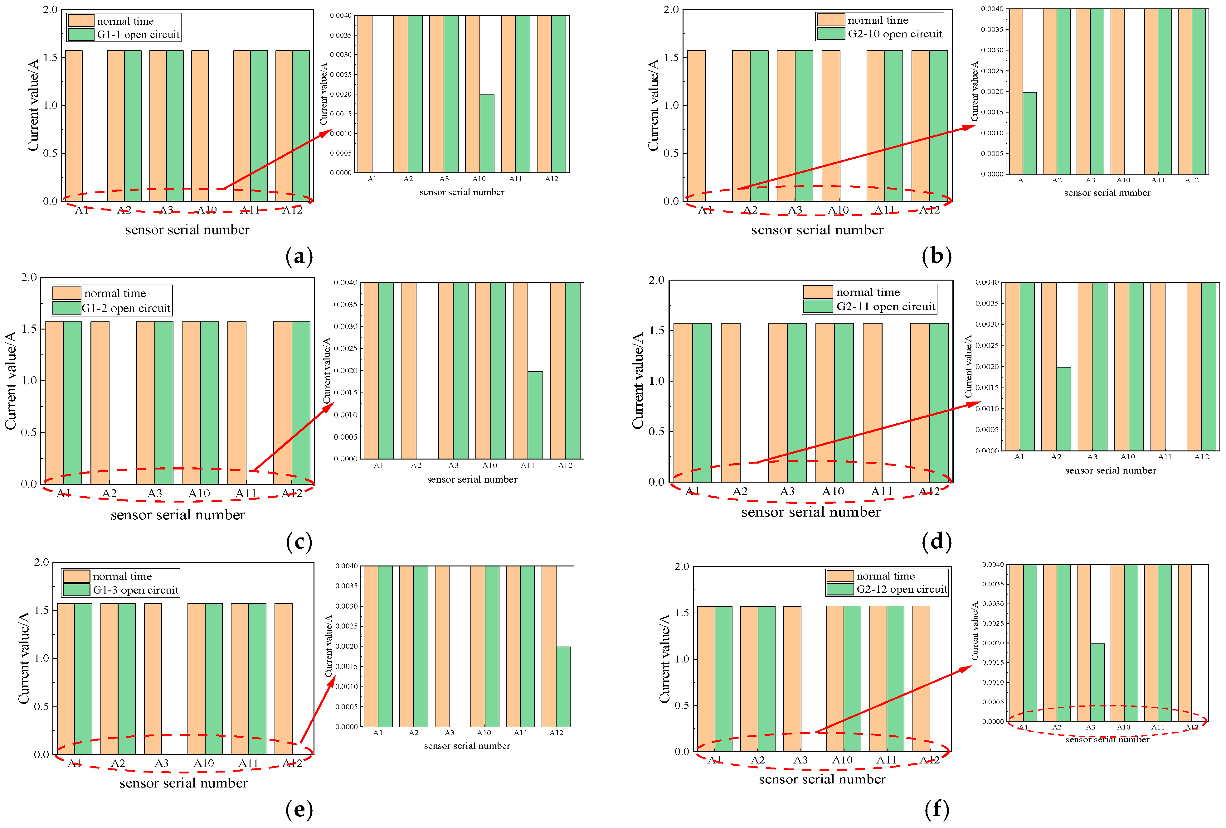
The disconnection of the grounding wire of the metal sheath of the grounding box results in the simulation of an open-sheath fault. The simulation demonstrated that when the grounding box sheath is open circuit, the sheath circuit current and branch circuit resistive current are identical to their normal values. Consequently, it is not possible to diagnose an open-circuit fault in the grounding box by monitoring the branch circuit resistive current and sheath current alone. Instead, it is essential to analyze the value of each current transformer at the time of the fault to provide a criterion for diagnosis. The simulation results are presented in Figure 10.
Figure 10.
Open-circuit fault of inner sheath of grounding box. (a) Open branch circuit of the sheath where A1 is located in G1; (b) Open branch circuit of the sheath where A10 is located in G2; (c) Open branch circuit of the sheath where A2 is located in G1; (d) Open branch circuit of the sheath where A11 is located in G2; (e) Open branch circuit of the sheath where A3 is located in G1; (f) Open branch circuit of the sheath where A12 is located in G2.
Figure 10 illustrates that G1-1 denotes the sheath branch linked to transformer A1 at the outlet end of grounding box G1. The serial numbers depicted in the figure correspond to the numbers of the current transformers, which align with those displayed in Figure 1. In the event of an open-circuit fault in the grounding box, the current transformer connected to the branch in question exhibits a measured value of zero. Conversely, the current transformer situated at the opposite end of the branch is indicative of the residual current leakage from the cable. Consequently, utilizing data from A1, A2, A3, A10, A11, and A12 enables the precise localization of the open-sheath fault within the grounding box.
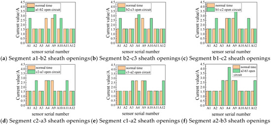
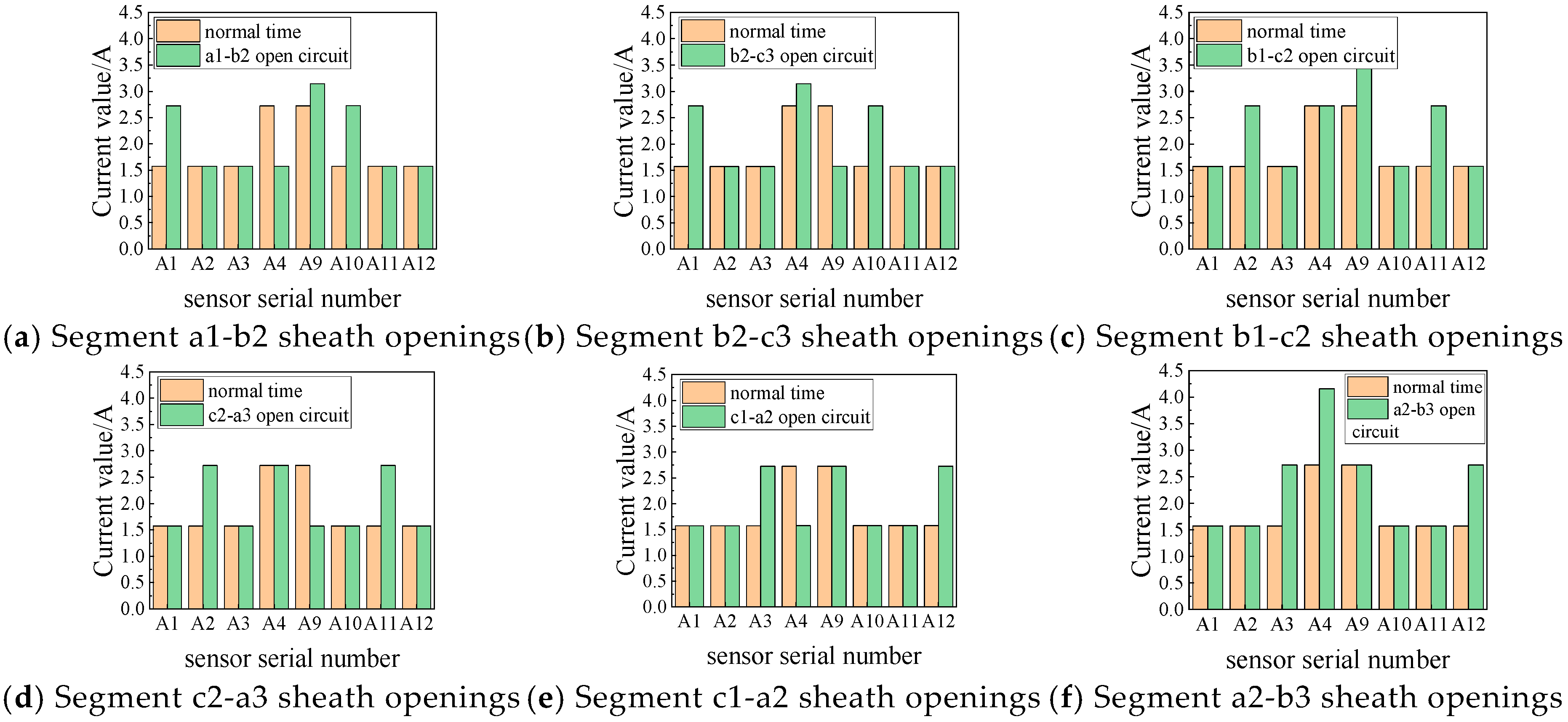
When the metal sheath outlet in the cross-bonding link box is disconnected to simulate an open-circuit fault, the current measured by the current transformer installed at the outlet end of the cross-bonding link box is the vector sum of the currents in the metal sheath of the small sections of the cable of the same phase. The simulation of open-circuit faults at the outlet end of the cross-bonding link box revealed that, with identical open-circuit faults in the grounding box, the various sheath circuit currents and the various branch resistive currents remained consistent. However, the current transformer’s measured value exhibited a discernible pattern of change. This observation aligns with the predictions of Equations (9) and (10). The measured values of current transformers A4, A5, and A6 were found to be zero, as were the measured values of current transformers A7, A8, and A9. Therefore, it was deemed sufficient to explore the laws governing current transformers A1 through A4 and current transformers A9 through A12 by examining the simulation results for the measured values of each current transformer, as illustrated in Figure 11.
Figure 11.
Current transformer current of open-circuit fault in the inner sheath of transposition box.
As illustrated in Figure 11, when the sheath circuit a1-b2-c3 is in the open-circuited state within the cross-bonding link box N1, the currents flowing through the current transformers A1, A9, and A10 will increase, while the current flowing through transformer A4 will decrease. The remaining current transformer values will remain unaltered. This phenomenon occurs because when the a1-b2 section is open circuit, the leakage current of the cable’s small section a1 does not shunt all the flow through the transformer A1. Instead, the grounding line into the earth, b2 section, and c3 section of the leakage current through the current transformer A9 and A10 flow into the earth. Regarding the sensor A4, the current measured by the original two sections of the sheath current vector becomes a section of the current flow, resulting in a reduction. The sheath circuit current of a1-b2-c3 does not flow through transformers A2, A3, A11, and A12. Therefore, the open circuit of the a1-b2 sheath has no effect on its measured value. When the cross-bonding link box N2 within the protective circuit b2-c3 section opens, the current flowing through transformers A1, A4, and A10 will increase, while the current flowing through the transformer A9 will be reduced. The remaining transformer currents will remain unchanged. This is because when the b2-c3 section is open circuit, the leakage current of the cable segment c2 does not shunt all of the flow through the transformer A10, where the grounding line into the earth is situated. Additionally, the leakage current through the current transformers A1 and A4 into the earth is distributed between the a1 section and the b2 section. Regarding sensor A9, the current measured by the original two sections of the sheath current vector represents only a portion of the total current flow, thus exhibiting a reduction. It should be noted that the same sheath loop a1-b2-c3 current does not flow through the transformers A2, A3, A11, and A12. Consequently, the b2-c3 sheath open circuit does not affect the measured value of the sensor A9. The analysis of an open circuit in the sheath is analogous.
5.3. Cross-Bonding Link Box Immersion Short-Circuit Fault
The transposition box immersion short-circuit fault is primarily caused by damage or poor sealing of the transposition box body, which allows sewage to enter the box and causes a short circuit. A phase metal sheath to ground the short circuit will not result in alterations to the leakage current in the insulation. Consequently, the branch circuit resistive current and the phase of the loss factor of the dielectric remain unaltered.
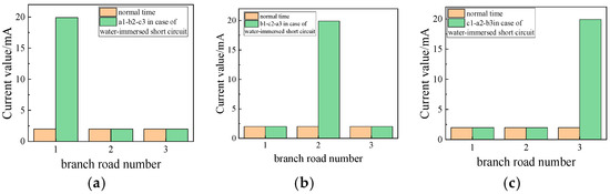
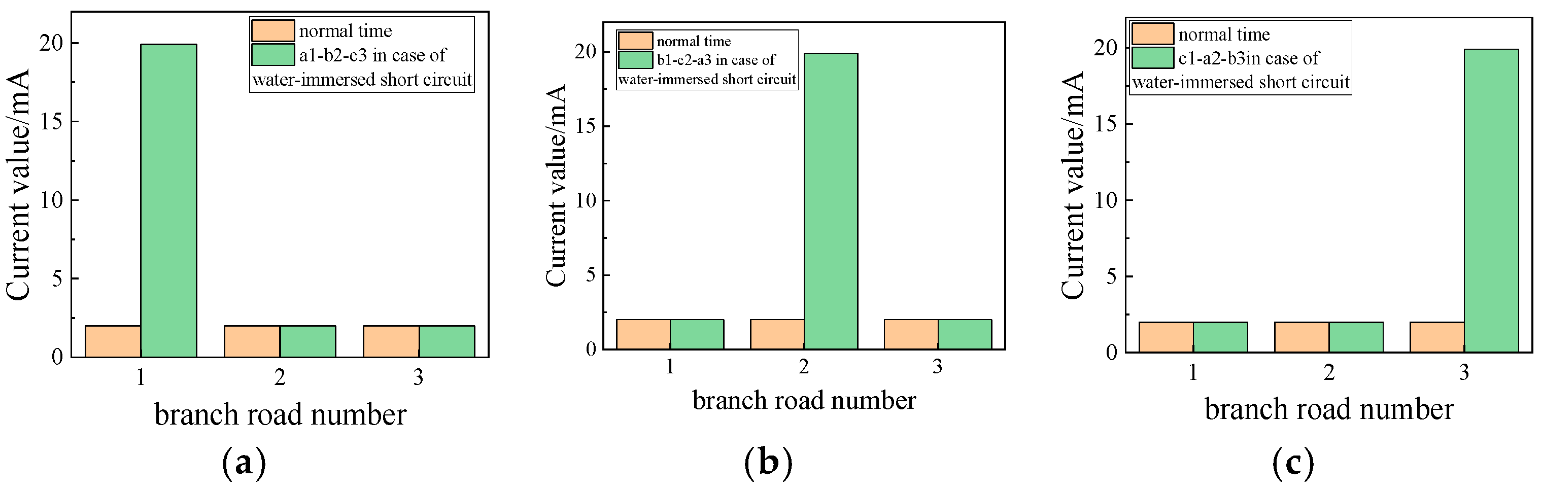
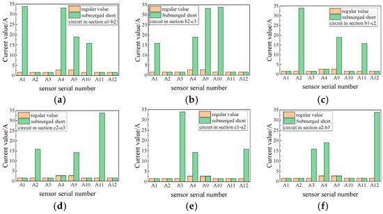
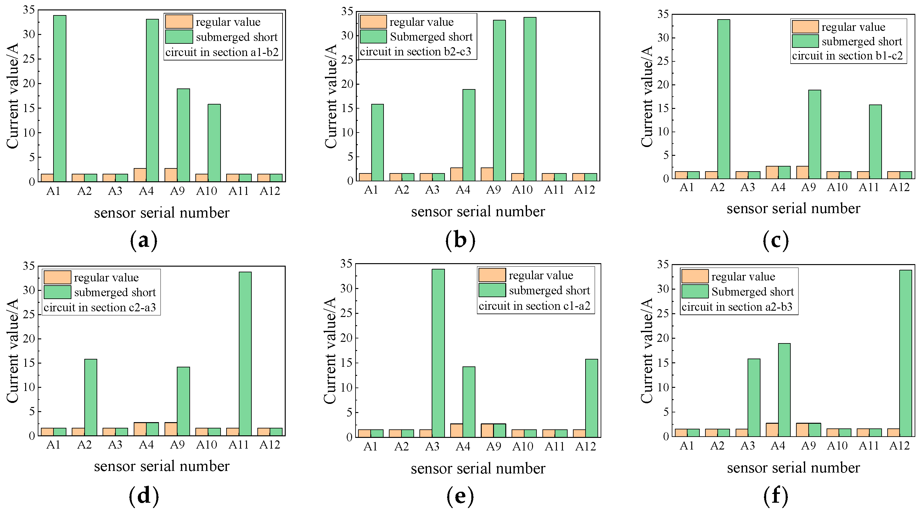
Nevertheless, the cross-bonding link box immersion short-circuit fault alters the configuration of the sheath circuit, resulting in a modification of the sheath circuit current. Two small sections of cable wiring should be set directly to ground to simulate the cross-bonding link box immersion short-circuit fault. As illustrated in Figure 12, the occurrence of a short-circuit fault results in a notable increase in the sheath current of the circuit where the fault originates. This is attributed to the short-circuit effect induced by a change in the structural configuration of the sheath circuit, which in turn leads to the generation of an induced voltage. In the event of a fault in the sheath circuit, the current in the sheath circuit becomes imbalanced, resulting in a significant increase in current flow. In such instances, it is essential to combine a switching box with a change in the value of the current transformer to ascertain the precise circumstances. The simulation outcomes are illustrated in Figure 13.
Figure 12.
Transposition box immersion short-circuit fault branch sheath circuit current. (a) a1-b2-c3 branch water immersion short circuit; (b) b1-c2-a3 branch water immersion short circuit; (c) c1-a2-b3 branch water immersion short circuit.
Figure 13.
Water immersion short-circuit fault in transposition box. (a) Short-circuiting of a1-b2 sheath inundation; (b) Short-circuiting of b2-c3 sheath inundation; (c) Short-circuiting of b1-c2 sheath inundation; (d) Short-circuiting of c2-a3 sheath inundation; (e) Short-circuiting of c1-a2 sheath inundation; (f) Short-circuiting of a2-b3 sheath inundation.
As illustrated in Figure 12 and Figure 13, the occurrence of an inundation ground fault in a sheath circuit within the cross-bonding link box is accompanied by a rapid increase in the current within the circuit where the fault originates. The transformer current on the side of the grounding box connected to the location of the short circuit and in proximity to the short circuit increases rapidly by a significant factor, thereby enabling the specific location of the inundation short-circuit fault to be determined.
5.4. Cable Tap Breakout Faults
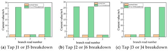
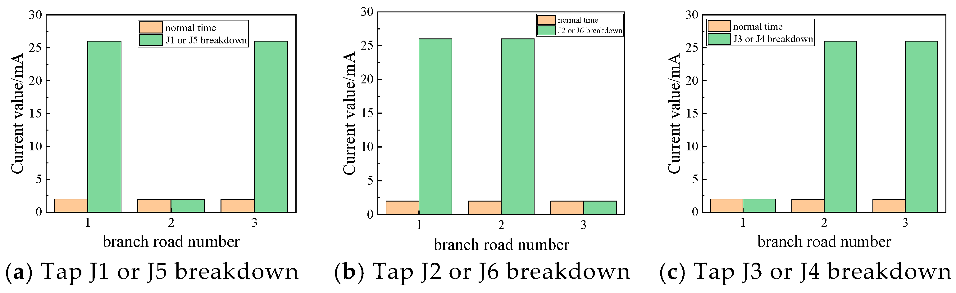
If a cable tap is not installed in accordance with the relevant specifications or is of an inferior quality, the tap is susceptible to insulation failures, which may result in a short circuit between the two sheaths. The occurrence of a short-circuit failure results in a modification of the circuit topology between the two sheaths, thereby establishing a novel current path. Figure 1 illustrates that if the cable tap J1 and J5 fail, they will not cause a shortage between the sheath circuit a1-b2-c3 and the sheath circuit c1-a2-b3. This results in the two sheath circuit currents being affected, while the other sheath circuit current remains unchanged. This is the same reason for other tap failures. The occurrence of this fault does not result in a change in the leakage current in the insulation; thus, the branch resistance currents and the dielectric loss factor of each phase remain unaltered. Due to the alteration in the structure of the sheath circuit, the sheath current will exhibit a discernible pattern. To simulate the cable tap breakdown fault, the two distinct metal sheath circuit outlets are shorted, and the resulting simulation results are presented in Figure 14.
Figure 14.
The current law of each branch of the tap breakdown fault.
As illustrated in Figure 14, the occurrence of a cable tap breakdown fault is indicated by a notable increase in the currents of the associated sheath circuits. The monitoring of these changes allows for the identification of a potential tap breakdown fault. However, the specific circuit involved in the fault remains undetermined. The law of sheath currents does not provide sufficient information to ascertain the location of the fault within the cable tap. In order to ascertain the simulation results depicted in Figure 15, it is essential to combine the alterations in the values of each current transformer.
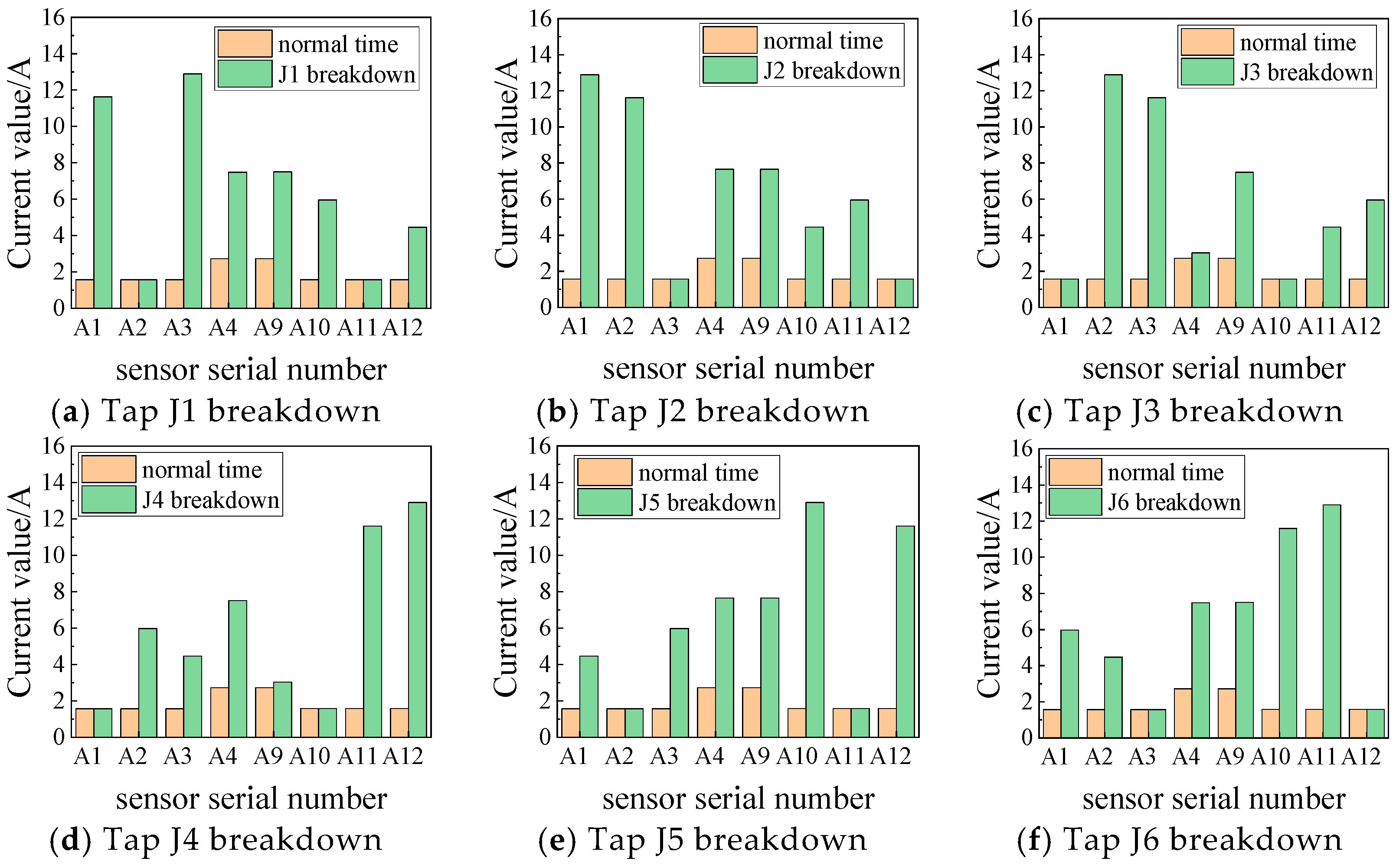
Figure 15.
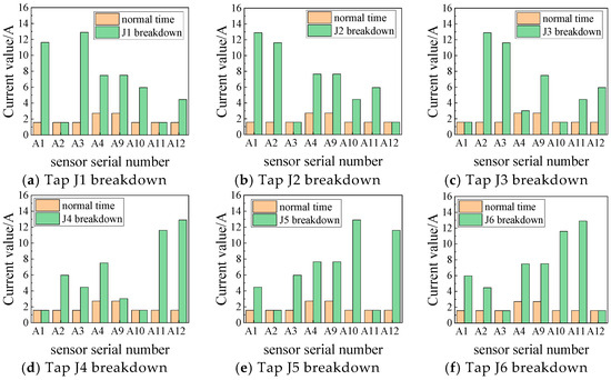
Breakdown fault of cable tap.
As illustrated in the figure, when tap J1 experiences a breakdown, the A-phase cable a1 and a2 sections of the metal sheath are shorted. Consequently, the a1 and a2 sections are directly connected, and the distance between the current transformer A1 and A3 measurement value increases, becoming more apparent. Similarly, other tap breakdown faults exhibit a similar pattern.
5.5. Fault Types and Equivalent Model Characterization
All faults in this paper are realized by adjusting the equivalent circuit parameters or reconstructing the topology. The switching module with internal resistance is not used to avoid the transient interference caused by the switching action, and the steady-state fault characteristics are focused. The specific simulation logic is as follows: Insulation faults such as cable insulation faults and intermediate-joint breakdown, by adjusting the values of insulation equivalent resistance R and capacitance C, simulate insulation degradation or the breakdown state; topological faults such as sheath open circuit, transposition box immersion short circuit, and cable intermediate-joint breakdown, by disconnecting the circuit, shorting the node, or reconstructing the circuit connection mode, simulate sheath fracture, box short circuit, and other structural abnormalities; all fault simulations are based on the equivalent circuit model of the cross-connected unit established in the original text, maintaining the consistency of the core topology framework, and only modifying the fault-related local parameters or connection relationships. The selection of insulation resistance 1 MΩ corresponds to the serious insulation deterioration state, which is 0.56% of the normal insulation resistance 179 MΩ, which meets the industry operation and maintenance standard that the insulation resistance is lower than 10 MΩ and needs urgent maintenance. When the equivalent capacitance of 120 nF is insulation deterioration, there are defects such as pores and moisture in the insulation layer, which leads to the increase in capacitance value. Combined with the simulation sensitivity analysis, 1.5 times of the normal capacitance value of 78.8 nF is selected, which not only reflects the fault characteristics, but also avoids the non-convergence of simulation caused by parameter mutation. In this model, the arc resistance is not set separately, and the research focuses on the steady-state fault diagnosis, rather than the transient process at the moment of fault occurrence. The arc phenomenon belongs to the millisecond transient discharge, and the influence on the steady-state characteristic parameters of resistive current and dielectric loss factor can be ignored. The equivalent resistance of severe insulation fault has included the leakage current path characteristics of the fault point, and its value has equivalently reflected the conductive state after insulation breakdown, which is in the same order of magnitude as the equivalent resistance after arc stability, without additional superposition.
5.6. Fault Warning Threshold and Warning Mechanism
The sensitivity coefficient of the dielectric loss factor to early insulation deterioration is the highest, and the increase in the mild fault stage is more than 39%. Auxiliary warning parameters: resistive current is moderately correlated with insulation deterioration, which is used to verify the effectiveness of the core parameters warning; the reference value is derived from the normal state simulation data from the original Table 4 and Table 5, which ensures the consistency of the threshold setting: the reference value of the dielectric loss factor is 0.02256% of the three-phase mean value, and the reference value of the resistive current is 1.842 mA of the mean value of each branch; normal fluctuation range: it is determined by simulation steady-state monitoring that the dielectric loss factor fluctuation is ≤±5%, and the resistive current fluctuation is ≤±8%. The parameter variation law of insulation resistance from the 179 MΩ normal state to 50 MΩ early deterioration, 10 MΩ moderate deterioration, and 1 MΩ serious fault is extracted, and the two-stage early warning + fault confirmation mode is adopted, taking into account the timeliness and accuracy of early warning. For the first-level warning corresponding to mild deterioration, the dielectric loss factor is 1.10 to 1.30 times the reference value, that is, 0.0248% to 0.0293%; the resistive current is 1.15 times to 1.40 times the reference value, that is, 2.12 mA to 2.58 mA. At this time, the insulation resistance is between 30 MΩ and 50 MΩ, which is 16.8% to 27.9% of the reference value. The core parameters are slightly overrun, and the auxiliary parameters fluctuate synchronously, but do not reach the fault state. For the secondary warning corresponding to moderate deterioration, the dielectric loss factor is 1.30 to 1.50 times the reference value, that is, 0.0293% to 0.0338%; the resistive current value is 1.40 times to 1.70 times the reference value, that is, 2.58 mA to 3.13 mA. At this stage, the insulation resistance is between 10 MΩ and 30 MΩ, which is 5.6% to 16.8% of the reference value. Both parameters are significantly overrun, and the parameter change rate is not less than 5%/day. For the fault confirmation corresponding to severe deterioration, the dielectric loss factor is not less than 1.50 times the reference value, that is, not less than 0.0338%. The resistive current is not less than 1.70 times the reference value, that is, not less than 3.13 mA. At this time, the insulation resistance does not exceed 10 MΩ, and the parameters are greatly exceeded. The validity of the threshold is verified: the dielectric loss factor is 0.0315% and the resistive current is 2.45 mA for the early deterioration sample of insulation resistance 50 MΩ, which falls in the first-level warning interval and triggers accurately. The dielectric loss factor is 0.0398% and the resistive current is 2.92 mA for the moderately deteriorated sample with an insulation resistance of 10 MΩ, which falls in the second-level warning interval and has no missed judgment. The normal fluctuation sample with a dielectric loss factor of 0.0236% and a resistive current of 1.97 mA did not trigger an early warning to avoid misjudgment.
6. Discussion
The simulation results in Section 5 show that the three characteristic parameters—resistive current, dielectric loss factor, and sheath loop current—show different sensitivities to different fault types, which are closely related to the fault mechanism and cable cross-connect structure. For cable insulation fault Section 5.1, the dielectric loss factor shows the highest sensitivity. When the insulation resistance of a small section of insulation degradation is reduced to 1 MΩ, the dielectric loss factor of the corresponding phase is increased from 0.02256% to more than 0.0316% compared with the normal state, which is increased by more than 40%, while the resistive current is increased by about 30%, and the sheath circuit current is increased by about 25%. This is because the dielectric loss factor directly reflects the energy loss of the insulating material and is more sensitive to the early deterioration of the insulation than the absolute value of the resistive current. In contrast, the method of only using sheath current as the monitoring parameter cannot effectively distinguish the early insulation deterioration and the small fluctuation of sheath current, resulting in a high false alarm rate. For the metal sheath open-circuit fault Section 5.2, the current of the sheath loop itself does not change significantly, but the measured value of the specific current transformer shows obvious characteristics. Our method solves this problem by analyzing the combination of CT measurements and improves the diagnostic accuracy of open-circuit faults. For the transposition box immersion short-circuit fault and the cable tap breakdown fault of Section 5.3 and Section 5.4, the sheath loop current shows a significant increase, which is more than 50% higher than the normal state, while the resistive current and the dielectric loss factor remain almost unchanged. This is because these two types of faults mainly change the topology of the sheath circuit without affecting the insulation performance of the main insulation. Our method combines the changes in CT measurements at different positions to achieve fault location with an error of less than 0.1 km.
Compared with the existing research methods, this method has a wider fault coverage, covering four typical faults of cross-linked cables, while most of the existing methods only focus on 1–2 fault types. It has higher positioning accuracy, and the fault location error is controlled at ±0.1 km, which is better than most existing methods. Based on analytical derivation, this method avoids complex neural network training or parameter optimization and is more suitable for engineering applications.
7. Conclusions
This paper puts forth a methodology for assessing the insulation condition of cables through the analysis of sheath current, resistive current, and dielectric loss factors. By establishing an equivalent model of a high-voltage cable cross-interconnection unit and conducting a simulation analysis, the following conclusions are reached:
- (1)
- The methodology presented in this paper entails the calculation of the sheath current for each sheath circuit, which is subsequently analyzed through the lens of an equivalent circuit. This enables the isolation of the resistive current and the calculation of the dielectric loss factor.
- (2)
- A simulation model of the cross-interconnection unit has been developed, and the simulation results demonstrate the feasibility of using the resistive current, dielectric loss factor, and sheath loop current calculated from the measured values of the current transformer as the monitoring parameters for insulation monitoring.
- (3)
- In order to test the efficacy of the proposed insulation monitoring method, a series of simulations and analyses have been conducted on a range of cable insulation faults, including sheath open-circuit faults, transposition box immersion short-circuit faults, and tap breakdown faults. The results of these simulations demonstrate the accuracy of the proposed method and provide a foundation for the discrimination of faults based on the simulation outcomes.
Survivability Extension of Online Monitoring System: Anti-harsh environment design: adapted to the wet cable tunnel, directly buried soil corrosion, and other scenarios, the sensor adopts the IP68 protection level package, and the core monitoring module has a wide temperature range of −40 °C~85 °C to ensure continuous operation in extreme environments. The fault-tolerant mechanism of network disconnection: the edge storage unit is deployed locally, the characteristic parameter data within 1 month is cached when the network is disconnected, and the data is automatically transmitted after the network is restored to avoid data loss. Fault self-diagnosis function: the system regularly checks the status of the CT, voltage sensor, and communication link; automatically switches the standby channel when the equipment fails; and issues an equipment maintenance alarm to ensure that the monitoring is not interrupted. Compatibility extension: it supports docking with existing power SCADA systems and condition-based maintenance platforms, adopts the standard IEC 61850 communication protocol, does not need to reconstruct the existing scheduling system, and reduces deployment resistance.
Author Contributions
Conceptualization, C.W., D.Z., L.T., Z.Q. and B.Z.; Methodology, C.X.; Software, C.X.; Writing—original draft, C.W.; Writing—review & editing, B.Z.; Validation, Z.Q.; Supervision, D.Z.; Funding acquisition, B.Z. All authors have read and agreed to the published version of the manuscript.
Funding
This research was supported by the State Grid Heilongjiang Electric Power Company Limited Technology Project (Research on Key Technologies for Online Monitoring and Fault Diagnosis of Cross-connected Cable Insulation Based on the Separation of Resistive Current and Sheath Current) (NO.522437250005).
Data Availability Statement
The original contributions presented in this study are included in the article. Further inquiries can be directed to the corresponding author.
Conflicts of Interest
Authors Chunming Wei, Dewen Zhang, Chao Xu, Long Tan and Zhongzhi Qu were employed by the company State Grid Heilongjiang Electric Power Company Limited. The remaining authors declare that the research was conducted in the absence of any commercial or financial relationships that could be construed as a potential conflict of interest.
References
- Zhou, X.; Xia, X.; Xia, J.; Chen, S.; Zhang, Y.; Yang, L.; Luo, Y.; Wang, R.; Liu, X. On-line monitoring of high-voltage transmission cables based on a new criterion based on sheath current. China Electr. Power 2021, 54, 45–54. [Google Scholar]
- Sheng, B.J.; Zhou, C.K.; Donald, H.M.; Dong, X.; Peers, G.; Zhou, W. Partial Discharge Pulse Propagation in Power Cable and Partial Discharge Monitoring System. IEEE Trans. Dielectr. Electr. Insul. 2014, 21, 948–956. [Google Scholar] [CrossRef] [Scilit]
- Huang, H.K. 110kV XLPE Power Cable Insulation On-Line Monitoring Research. Master’s Thesis, Wuhan University, Wuhan, China, 2009; pp. 2–10. [Google Scholar]
- Dong, X.; Yuan, Y.L.; Gao, Z.; Zhou, C.; Wallace, P.; Alkali, B. Analysis of Cable Failure Modes and Cable Joint Failure Detection via Sheath Circulating Current. In Proceedings of the 2014 IEEE Electrical Insulation Conference (EIC), Philadelphia, PA, USA, 8–11 June 2014; pp. 294–298. [Google Scholar]
- Xu, Y.K.; Tian, Z. Research and application of induced voltage and current in shielding layer of single-core flexible cable. Autom. Appl. 2023, 64, 138–140. [Google Scholar]
- Cong, Q. Analysis of the influence of arrangement on reducing the induced voltage of cable metal sheath. Shandong Electr. Power Technol. 2019, 46, 42–46. [Google Scholar]
- Zhu, X.; Du, B.; Zhou, F.; Gao, Y.; Li, Z.; Ma, Z.; Tang, Q.; Gan, Y. Research status of on-line monitoring and detection technology for high voltage cross-linked polyethylene cable. Insul. Mater. 2009, 42, 58–63. [Google Scholar]
- Mao, Z.; Wu, Z.; Wu, Y.; Wang, P.; Du, X. Analysis of on-line monitoring methods for power cable insulation. Electromechanical Inf. 2019, 30, 6–8. [Google Scholar]
- Zhang, H.; Guan, W.; Guan, Z. Research on on-line diagnosis technology of cross-linked XLPE cable insulation based on ART2A-E. High Volt. Appar. 2010, 46, 48–52. [Google Scholar]
- Yang, L.T.; Tang, Z. Model analysis and calculation of single-core XLPE cable cross-connection. East China Electr. Power 2014, 42, 1629–1633. [Google Scholar]
- Yuan, Y.; Zhou, H.; Dong, J.; Shi, X.; Mu, Y.; Tang, Z.; Zhou, C. Online monitoring and fault diagnosis technology of high voltage power cable sheath current. High Volt. Technol. 2015, 41, 1194–1203. [Google Scholar]
- Zhou, W.; Yang, Y.; Wei, L.; Zhou, C.; Jiang, W.; Tang, Z. Application of leakage current separation and relative change monitoring of phase-to-phase dielectric loss in cross-connected cables. High Volt. Technol. 2016, 42, 468–477. [Google Scholar]
- Yang, J.; Zhu, X.; Dong, X.; Lu, Y.; Li, N. On-line Monitoring and Diagnosis of HV Cable Faults Based on Sheath Currents. High Volt. Eng. 2016, 42, 3616–3625. [Google Scholar]
- Zhu, B.; Yu, X.; Tian, L.; Yu, X.; Tian, L.; Wei, X. Cross-connected cable insulation monitoring and diagnosis based on resistive current and sheath current. J. Electr. Mach. Control 2023, 27, 79–88. [Google Scholar]
- Lai, S.; Xia, C.; Chi, Z.; Ji, H.; Chen, X.; Huang, L. Calculation and analysis of circulating current in metal sheath of high voltage cable considering leakage current and interlayer coupling. High Volt. Technol. 2024, 50, 765–774. [Google Scholar]
- Li, L.; Yong, J.; Zeng, L.; Wang, X.; Lu, J. On-line monitoring of overall aging of cross-linked cable insulation based on system power disturbance. J. Electr. Technol. 2018, 33, 3396–3405. [Google Scholar]
- Du, B.; Li, Z.; Zhang, K.; Wang, L. Calculation and application of grounding current of 220kV XLPE power cable. High Volt. Technol. 2013, 39, 1034–1039. [Google Scholar]
- Zhang, L.; Sheng, B.; Jiang, W.; Zhou, W.; Tian, Z.; Dong, X.; Tang, Z. On-line Partial Discharge Localization in Cross-bonded HV Cable Systems. High Volt. Eng. 2015, 41, 2706–2715. [Google Scholar]
- GB50217-2007; Power Engineering Cable Design Specification. Ministry of Construction of the People’s Republic of China; China Electric Power Press: Beijing, China, 2013.
- Wei, X.; Zhu, B.; Pang, B.; Wang, S.; Li, R. On-line Insulation Monitoring Method for Long Distance Three-Phase Power Cable. Proc. CSEE 2015, 35, 2079–2086. [Google Scholar]

Disclaimer/Publisher’s Note: The statements, opinions and data contained in all publications are solely those of the individual author(s) and contributor(s) and not of MDPI and/or the editor(s). MDPI and/or the editor(s) disclaim responsibility for any injury to people or property resulting from any ideas, methods, instructions or products referred to in the content. |
© 2026 by the authors. Licensee MDPI, Basel, Switzerland. This article is an open access article distributed under the terms and conditions of the Creative Commons Attribution (CC BY) license.