Low-Carbon Economic Dispatch of Data Center Microgrids via Heat-Determined Computing and Tiered Carbon Trading

Abstract

The exponential growth of the digital economy has transformed data centers into major energy consumers, yet their inflexible power consumption patterns and substantial waste heat generation pose significant challenges to grid stability and carbon neutrality targets. Existing energy management strategies often overlook the deep coupling potential between computing workload flexibility, thermal dynamics, and carbon trading mechanisms, leading to suboptimal resource utilization. To address these issues, this study proposes a collaborative low-carbon economic scheduling strategy for data center microgrids. A multiple-dimensional coupling framework is established, integrating a queuing theory-based model for delay-tolerant workload shifting and a heat-determined computing mechanism for active waste heat recovery (WHR). Furthermore, a mixed-integer linear programming (MILP) model is formulated, incorporating a linearized tiered carbon trading mechanism to facilitate source–load coordination. Simulation results demonstrate that the proposed strategy achieves a dual optimization of economic and environmental benefits, reducing total operating costs by 11.7% while minimizing carbon emissions to 6879 kg compared to baseline scenarios. Additionally, by leveraging temperature aware load migration, the daily weighted power usage effectiveness (PUE) is optimized to 1.2607. These findings quantify the marginal benefits of load flexibility under tiered pricing, providing insights for operators to balance service timeliness and energy efficiency in next generation green computing infrastructure.

1. Introduction

Driven by the imperative of addressing global climate change and promoting the carbon peaking and carbon neutrality strategy, constructing a new power system dominated by renewable energy has become the core direction of energy structure transformation [1,2]. Meanwhile, the digital economy driven by artificial intelligence, big data, and the Internet of Things is also experiencing rapid development, establishing computing power as a new factor of production [3]. However, the data center (DC), the main carrier of computing power, is characterized by intensive energy consumption. Currently, the annual power consumption of DCs worldwide exceeds 400 TWh, accounting for 1% to 2% of the global electricity consumption, and is expected to maintain exponential growth over the coming decade [4,5,6]. Due to high-density server clusters, not only is a substantial electrical load imposed, but significant carbon emissions also arise from the continuous operation of cooling systems [7,8]. Consequently, the traditional unidirectional power supply architecture is unable to balance economic efficiency and low carbon emissions under the increasing demand for high computing power; this limitation further exacerbates the peak-valley load spread and intensifies the peak regulation pressure on the distribution network [9]. Therefore, establishing a data center microgrid (DCMG) that integrates distributed energy resources and features source–load interaction capabilities has emerged as a promising solution for realizing green computing power [10,11].

The existing research on distributed energy management in DCMG primarily concentrates on the energy supply side. This research typically adopts the framework concept of integrated energy systems and integrates components such as microturbine (MT), combined cooling, heating, and power (CCHP) systems, energy storage systems (ESSs), and other equipment to enhance energy utilization efficiency [12,13,14]. For instance, a coordinated scheduling strategy for cooling, heating, and electrical loads was proposed in [15], primarily based on CCHP units to enhance primary energy efficiency. Additionally, references [16] introduced power-to-gas and carbon capture systems, respectively, aiming to improve the absorption capacity of renewable energy [17,18]. However, most existing studies model the DC as a rigid load, neglecting the spatiotemporal flexibility of computing tasks. This drawback is particularly critical under high photovoltaic (PV) penetration, where supply-demand mismatches often occur. Hence, the system is forced to rely heavily on energy storage or resort to renewable curtailment to maintain balance, leading to high capital expenditures and operating costs [19].

On the demand side of computing power, workload scheduling strategies targeting deferrable workloads have been widely adopted to optimize energy consumption or facilitate cross-regional electricity price arbitrage [20,21,22]. However, most existing studies utilize a linear power consumption model based on CPU utilization, which often oversimplifies the complex electro-thermal conversion mechanism associated with computational processes. Servers convert approximately 97% of the electricity they consume into low-grade heat [23]. In traditional air-cooled systems, this waste heat is directly dissipated, which not only results in energy waste but also intensifies the cooling load of the system [24,25]. Thus, developing approaches to efficiently recover waste heat generated by computing power scheduling and accurately match it with the heat load of the facility in both time and space is a pressing interdisciplinary challenge that must be addressed [26].

In terms of solving methodologies, early studies primarily relied on heuristic algorithms, such as particle swarm optimization and genetic algorithms, to address the scheduling problem of microgrids [27]. However, these algorithms are characterized by unstable convergence performance and a tendency to remain trapped in local optima. In contrast, MILP is frequently employed in scheduling strategies due to its ability to achieve global optimality and its robust computational efficiency [28]. When the carbon trading mechanism is incorporated, the carbon emission cost will present a piecewise nonlinear characteristic. This feature will render the scheduling model a nonconvex problem, increasing the complexity of modeling and solving, thereby not guaranteeing a global optimal solution. Additionally, existing research rarely investigates how computing power flexibility responds to carbon price signals, limiting the system’s ability to balance high computing power throughput with low carbon emissions [29,30].

However, existing DCMG scheduling frameworks still face critical limitations. Current approaches frequently overlook the deep coupling between computing workload flexibility and thermal dynamics by modeling the DC as a rigid load. Simultaneously, WHR strategies tend to be passive, failing to achieve active spatiotemporal coordination with thermal demand, which undermines energy cascading efficiency. Moreover, the lack of a unified framework integrating tiered carbon trading with source–load interaction restricts the system’s capacity to optimize the trade-off between computing throughput and carbon emissions under nonlinear pricing signals. These limitations undermine the physical coupling between computing power flow and heat flow. This results in an increased reliance on carbon-intensive gas boiler (GB) during peak heating demand periods, notably at night, while DC servers frequently operate at low load. This scenario impedes the exploitation of their waste heat potential, ultimately leading to a simultaneous waste of both energy and computing power resources.

In response to the identified research gaps, this study proposes a day-ahead low-carbon economic scheduling strategy for DCMG. This strategy integrates the temporal flexibility of computing workloads with the cascading utilization of waste heat, aiming to establish a deep coupling mechanism among the bit flow, watt flow, and heat flow. The main contributions of this study are as follows:

• A coupling model of computing power and energy is formulated based on queuing theory. By characterizing the dynamic backlog and service behavior of delay-tolerant workloads, the temporal flexibility of computing tasks is accurately mapped to schedulable electric and thermal loads, overcoming the limitations of traditional rigid load assumptions.
• A novel mechanism for cascade utilization of waste heat is proposed, based on heat-determined computing. This strategy reclaims waste heat from servers via a heat pump and actively remodels the temporal profile of computing workloads in alignment with thermal demand. This mechanism facilitates a deep coupling between computing workload scheduling and thermal energy utilization, transforming the DC into a schedulable, flexible heat source within the microgrid system.
• A source–load coordinated optimization strategy is developed based on a tiered carbon trading mechanism. The nonlinear piecewise carbon cost is linearized using the Big-M method to formulate a MILP model amenable to efficient solving, facilitating the joint optimization of energy complementarity, temporal shifting of computing workloads, and carbon cost constraints within a unified framework.

2. System Model

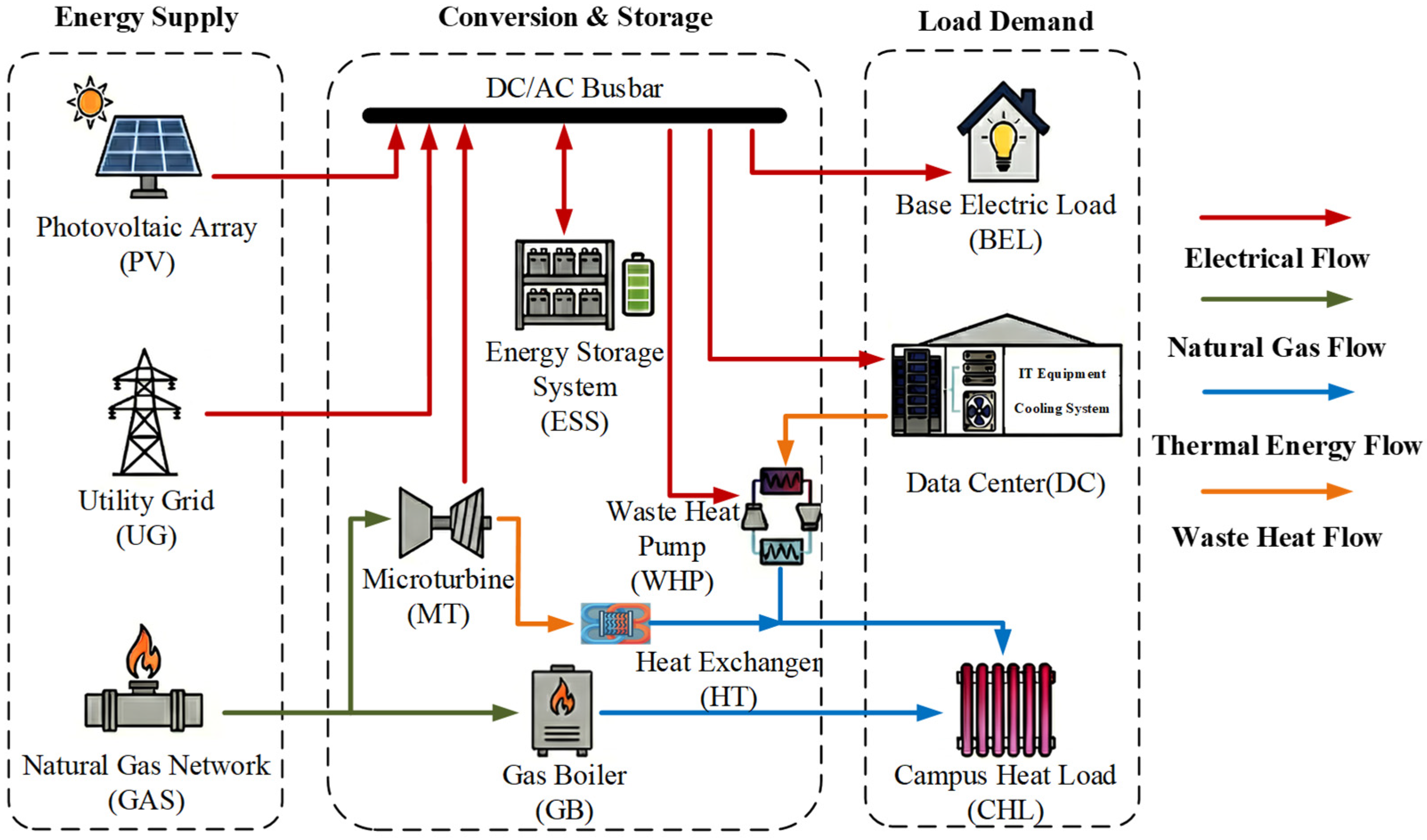
The DCMG in this study operates in a grid-connected mode, as illustrated in Figure 1. On the energy supply side, the system interfaces with the utility grid and the natural gas network to access external energy sources. Simultaneously, a PV array serves as the primary distributed renewable energy source. In the energy conversion and storage stage, the system aggregates various forms of electric energy through an AC/DC hybrid busbar. This integration includes an MT, a GB, and an ESS. Moreover, it establishes a cascade utilization architecture for thermal energy. Specifically, the high-temperature exhaust gas from the MT is efficiently recovered via a heat exchanger, while the low-grade waste heat generated by the DC is reclaimed by an electric waste heat pump (WHP). These components operate in conjunction with the GB to satisfy the campus heat load. Furthermore, the DC/AC hybrid busbar supplies power to the base electrical load (BEL) and the DC within the campus. The energy consumption of the DC consists primarily of two components: IT equipment and the cooling system. This configuration facilitates the deep physical coupling of computation, electricity, and thermal energy flows.

2.1. Computing–Energy Coupling Model of Data Center

The DC acts as the core dispatchable resource within the DCMG. Here, the transmission and processing of computing tasks are conceptualized as “bit flow,” representing the information load that interacts with the physical “watt flow” (electricity) and “heat flow” (thermal energy) within the coupled system. To quantify the flexibility of computing workloads, the total workload is classified into two categories: delay-sensitive workloads and delay-tolerant workloads. Specifically, queuing theory is applied to formulate a dynamic load model for delay-tolerant tasks, characterizing their potential for temporal shifting within specified time windows. In this study, the computing workload represents the service request arrival rate, measured in Tasks/h. It determines the server CPU utilization based on the cluster’s maximum processing capacity.

2.1.1. Workload Queuing Model

The dynamic update mechanism of the delay-tolerant workload queue is formulated as:

$$Q_{flex,t}=Q_{flex,t-1}+D_{flex,t}^{in}-D_{flex,t}^{proc},\hspace{1em}\forall t\in \mathcal{T},$$

(1)

where $Q_{flex,t}$ denotes the queue backlog of delay-tolerant tasks at the end of time slot $t$, $D_{flex,t}^{in}$ and $D_{flex,t}^{proc}$ represent the arriving workload and the actually processed workload during this period, respectively.

To guarantee quality of service, the queue length and processing rate must satisfy the following physical constraints:

$$0\le Q_{flex,t}\le Q_{max}^{buffer},$$

(2)

$$0\le D_{sen,t}+D_{flex,t}^{proc}\le N_{srv}\cdot f_{max},$$

(3)

where $Q_{max}^{buffer}$ denotes the maximum capacity of the task queue buffer. $D_{sen,t}$ represents the arrival workload of delay-sensitive workloads that require immediate processing during time slot $t$. $N_{srv}$ denotes the number of active servers, and $f_{max}$ indicates the maximum processing rate of a single server (Tasks/h).

To prevent task backlogs or losses within the scheduling horizon, the workload conservation constraint must be satisfied:

$${\displaystyle \sum _{t\in \mathcal{T}}{D}_{flex,t}^{proc}}={\displaystyle \sum _{t\in \mathcal{T}}{D}_{flex,t}^{in}}.$$

(4)

2.1.2. Server Energy Consumption

The resource utilization status of the server cluster must first be defined to establish the correlation between computing workloads and physical energy consumption. Assuming that task scheduling within the cluster satisfies load balancing conditions and that the processing rate is linearly correlated with computing resource usage, the average CPU utilization rate during time slot $t$, denoted as $u_{cpu,t}$, is modeled as the ratio of the current processing workload to the maximum processing capacity:

$$u_{cpu,t}={\displaystyle \frac{D_{sen,t}+D_{flex,t}^{proc}}{N_{srv}\cdot f_{max}}}.$$

(5)

Consequently, the total power consumption of the servers, $P_{serv,t}$, can be expressed as a linear function of the CPU utilization rate $u_{cpu,t}$:

$$P_{serv,t}=N_{srv}\cdot [P_{idle}+(P_{peak}-P_{idle})\cdot u_{cpu,t}],$$

(6)

where $P_{idle}$ and $P_{peak}$ represent the idle power consumption and peak power consumption of a single server, respectively.

Although the power consumption of individual servers exhibits nonlinear characteristics in practice, the linear approximation provides an acceptable trade-off between accuracy and computational complexity for system-level scheduling [12]. This linearization preserves the convexity of the problem, ensuring that the proposed MILP model can be solved efficiently with a global optimal guarantee.

2.1.3. Cooling System Model

The total power consumption of the DC, denoted as $P_{DC,t}$, consists of server power and cooling power. The cooling power consumption is not solely determined by the heat dissipation of IT equipment but is also highly sensitive to the ambient temperature, $T_{amb,t}$. To characterize this variable operating condition, this study utilizes the temperature-dependent coefficient of performance (COP), denoted as $COP(T_{amb,t})$. The total power model is formulated as:

$$P_{DC,t}=P_{serv,t}\cdot \left(1+{\displaystyle \frac{1}{COP(T_{amb,t})}}\right).$$

(7)

This formulation indicates that shifting a portion of computing workloads to nighttime, characterized by lower ambient temperatures, can enhance the COP, thereby effectively reducing cooling energy expenditure. Although COP-based model simplifies the complex thermodynamics of cooling systems (e.g., neglecting humidity variations and specific cooling architectures) but is widely adopted in microgrid dispatch problems to capture the primary impact of ambient temperature on energy efficiency [7]. While simplified, it sufficiently characterizes the hourly energy baseline for the proposed day-ahead optimization framework.

2.2. Energy Conversion and Storage Devices

2.2.1. Waste Heat Recovery Model

Assuming that the electrical energy consumed by servers is almost entirely dissipated as heat, the electro-thermal conversion coefficient is defined as ${\eta }_{heat}$. The waste heat generation can be expressed as:

$$Q_{waste,t}={\eta }_{heat}\cdot P_{serv,t},$$

(8)

where $Q_{waste,t}$ represents the total waste heat generated by the server cluster during time slot $t$.

To account for physical limitations in the recovery process, the actual thermal energy absorbed by the heat pump, denoted as $Q_{abs,t}$, is constrained by the capture efficiency constraint:

$$0\le Q_{abs,t}\le {\eta }_{cap}\cdot Q_{waste,t},$$

(9)

where ${\eta }_{cap}$ denotes the efficiency of capturing waste heat. In this study, the electro-thermal conversion efficiency ${\eta }_{heat}$ is set to 0.97, as suggested in [23]. The waste heat capture efficiency ${\eta }_{cap}$ is set to 0.80. This value represents a conservative benchmark for modern DCs with WHR capabilities [5]. Based on the law of conservation of energy, the total heat energy supplied to users by the heat pump, denoted as $Q_{rec,t}$, comprises the absorbed waste heat and the electrical power consumed by the compressor, $P_{WHP,t}$. Modeling the heating COP as $CO{P}_{WHP}$, the relationship is formulated as:

$$Q_{rec,t}=Q_{abs,t}+P_{WHP,t}=P_{WHP,t}\cdot CO{P}_{WHP}.$$

(10)

The equations presented above form the foundational principles of the heat-determined computing mechanism. Specifically, when there is an increase in thermal demand, the system can optimize the task and proactively increase computing workload allocation to boost the recovery of waste heat. This strategy enables the system to effectively meet heating demands by operating the heat pump efficiently.

2.2.2. Microturbine Model

As a dispatchable power generation unit, the output power of the MT in time slot $t$, denoted as $P_{MT,t}$, must satisfy the following capacity constraints to ensure safe operation:

$$u_{MT,t}{P}_{MT}^{min}\le P_{MT,t}\le u_{MT,t}{P}_{MT}^{max},$$

(11)

where $u_{MT,t}$ is a binary commitment variable (taking 1 for ON and 0 for OFF), while $P_{MT}^{min}$ and $P_{MT}^{max}$ represent the minimum stable output and maximum rated output of the MT, respectively.

To prevent equipment damage caused by frequent power fluctuations, the ramping rate is constrained to restrict the power variation between consecutive time slots:

$$-R_{ramp}^{MT}\le P_{MT,t}-P_{MT,t-1}\le R_{ramp}^{MT},$$

(12)

where $R_{ramp}^{MT}$ denotes the ramping rate of MT. This constraint aims to restrict the range of output changes between two consecutive periods, ensuring the MT operates smoothly and reliably.

In parallel, the MT functions as the core cogeneration unit within the microgrid. It generates electric power while the discharged high-temperature flue gas serves as a significant supplementary heat source. To characterize its thermoelectric coupling characteristics, this study assumes that MT operates with a fixed heat-to-power ratio, exhibiting a linear relationship between heat output and electric power output:

$$Q_{MT,t}=P_{MT,t}\cdot {\gamma }_{MT},$$

(13)

where $Q_{MT,t}$ represents the effective heating power in time slot $t$, and ${\gamma }_{MT}$ denotes the heat-to-power ratio. This equation reflects the device’s WHR capability per unit of power generation.

2.2.3. Gas Boiler Model

As a supplementary heat source within the DCMG, the GB is primarily utilized to compensate for thermal supply deficits when the recovered waste heat from the MT and other sources is insufficient to meet the campus thermal load. The heat generation process is characterized by its thermal conversion efficiency. Accordingly, the relationship between the generated heat power, $Q_{GB,t}$, and the consumed natural gas power, $P_{gas,GB,t}$, is formulated as:

$$Q_{GB,t}={\eta }_{GB}\cdot P_{gas,GB,t},$$

(14)

where ${\eta }_{GB}$ represents the thermal conversion efficiency of the GB.

To ensure operational safety, the thermal output of GB must satisfy the following capacity constraint:

$$0\le Q_{GB,t}\le Q_{GB}^{max},$$

(15)

where $Q_{GB,t}^{max}$ denotes the rated maximum heating power of the GB. In the context of the thermal power balance, the GB output is dispatched to mitigate heat load shortages. Consequently, the associated natural gas consumption and the resulting carbon emission are integrated into the system’s total operating cost objective.

2.2.4. Energy Storage System Model

The ESS facilitates peak shaving and valley filling through temporal energy shifting (charging and discharging across different periods). This study employs a generic state of charge (SOC) model to characterize its dynamic evolution:

$$E_{bat,t}=E_{bat,t-1}(1-\sigma )+\left({\eta }_{ch}{P}_{ch,t}-{\displaystyle \frac{P_{dis,t}}{{\eta }_{dis}}}\right)\Delta t,$$

(16)

where $E_{bat,t}$ denotes the energy stored in the ESS at time slot $t$, $\sigma$ represents the self-discharge rate, $P_{ch,t}$ and $P_{dis,t}$ represent the charging and discharging power in time slot $t$, respectively, while $\Delta t$ denotes the scheduling time interval. In this formulation, the charging energy is multiplied by the efficiency, while the discharging energy is divided by the efficiency, to strictly account for internal energy losses.

The charging and discharging powers are bounded by the following operational constraints:

$$0\le P_{ch,t}\le u_{ch,t}{P}_{ch}^{max},$$

(17)

$$0\le P_{dis,t}\le u_{dis,t}{P}_{dis}^{max},$$

(18)

where $u_{ch,t}$ and $u_{dis,t}$ are binary status variables indicating the charging and discharging states (1 for active, 0 for inactive). $P_{ch}^{max}$ and $P_{dis}^{max}$ represent the maximum allowable charging and discharging power, respectively.

To ensure safe operation, the capacity constraint is defined as:

$$0.1E_{bat}^{max}\le E_{bat}^{max}\le 0.9E_{bat}^{max}.$$

(19)

The SOC window of [10%, 90%] is selected to optimize the trade-off between capacity utilization and longevity. Physically, avoiding extreme states mitigates electrode stress [31] while retaining 80% effective capacity. Operationally, the upper margin serves as a buffer for unpredicted PV surpluses, enhancing system robustness.

Furthermore, to prevent the ESS from charging and discharging simultaneously within the same time slot, a complementarity constraint is imposed:

$$u_{ch,t}+u_{dis,t}\le 1.$$

(20)

This inequality constraint allows for the idle state (where $u_{ch,t}=0$ and $u_{dis,t}=0$), ensuring that the ESS can hold its energy state without charging or discharging when necessary.

Finally, to guarantee the sustainability of the scheduling cycle, the energy state at the beginning and the end of the period must remain consistent:

$$E_{bat,0}=E_{bat,T}.$$

(21)

While battery aging is physically nonlinear dependence on the depth of discharge, incorporating such non-convex characteristics would compromise the computational tractability of the global optimization. Therefore, this study adopts a linearized approach: deep discharge is physically prevented by the strict SOC constraints defined in Equation (19), while cycle degradation costs are implicitly amortized into the operation and maintenance coefficient (${\delta }_k$ in Equation (27)).

2.3. Power Balance Constraints

2.3.1. Electrical Power Balance

To guarantee the stable operation of the DCMG, the real-time balance between electrical supply and demand must be strictly maintained. The electrical power balance constraint is formulated as:

$$P_{PV,t}+P_{MT,t}+P_{grid,t}^{purchase}+P_{dis,t}=P_{DC,t}+P_{WHP,t}+P_{ch,t}+P_{BEL,t}+P_{loss,t},$$

(22)

where $P_{PV,t}$ denotes the output power of the PV system in time slot $t$, $P_{grid,t}^{purchase}$ represents the power purchased from the utility grid. $P_{BEL,t}$ represents the non-IT BEL of the campus, and $P_{loss,t}$ represents the aggregate power losses, calculated as 2% of the total electrical demand to account for transmission and conversion inefficiencies. This equation ensures that the aggregated power supply meets the total demand of all electrical loads, thereby maintaining the electrical equilibrium of the system.

2.3.2. Thermal Power Balance

Similarly, the system’s thermal balance is governed by the following constraint:

$$Q_{rec,t}+Q_{GB,t}+Q_{MT,t}=Q_{load,t}+Q_{loss,t},$$

(23)

where $Q_{load,t}$ is the total thermal load demand of the campus in time slot $t$, and $Q_{loss,t}$ denotes the thermal energy dissipation during transmission, set as 5% of the thermal load in the revised model. This equation indicates that the server waste heat recovered by the heat pump, the MT waste heat, and the supplementary heat from the boiler collaboratively satisfy the thermal load, thereby preserving the thermal equilibrium on the demand side.

3. Low-Carbon Economic Dispatch Considering Tiered Carbon Trading

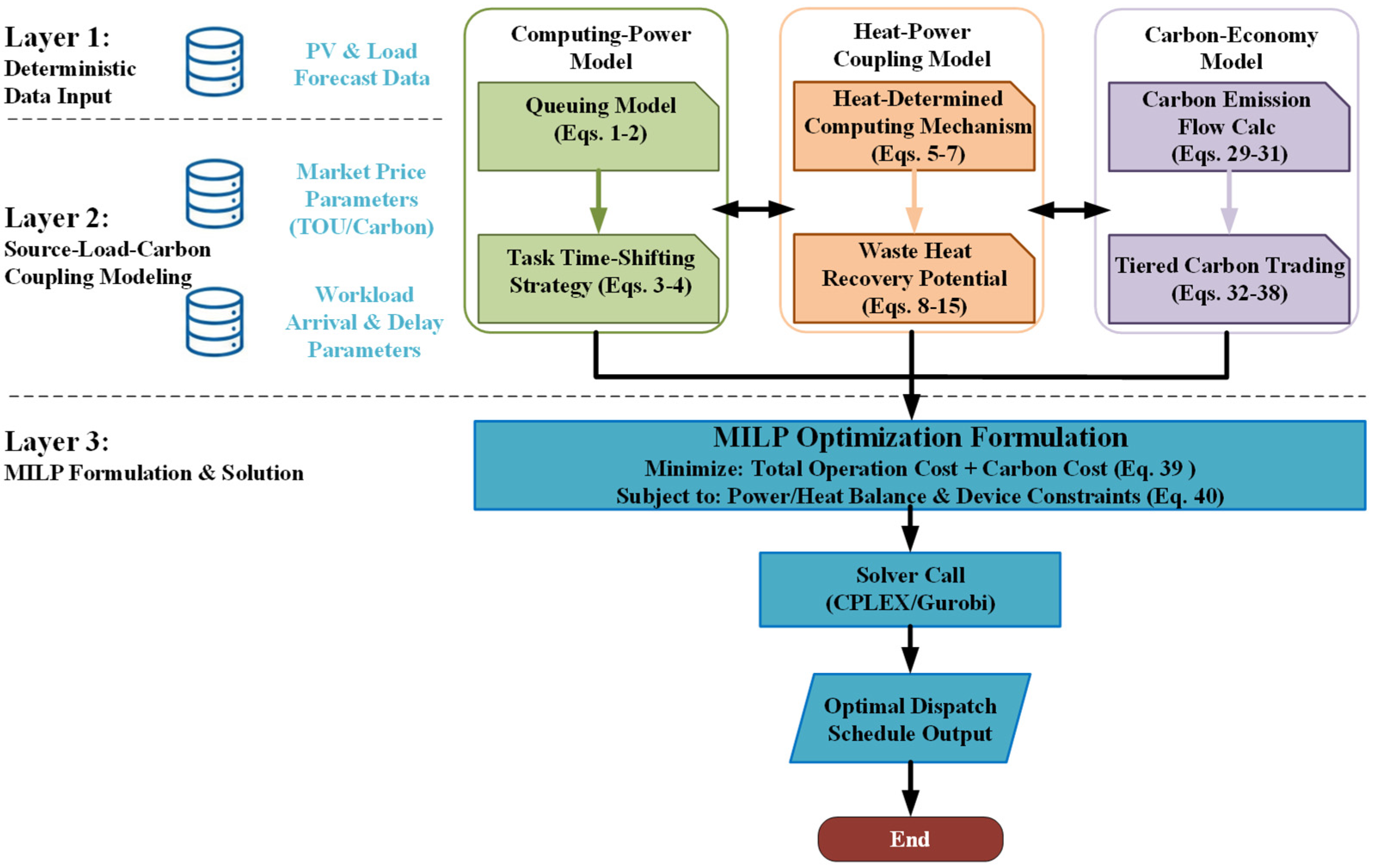
The low-carbon economic dispatch strategy proposed herein establishes a multiple-level architecture, as shown in Figure 2. This framework comprises three core layers: the deterministic data input layer, the source–load–carbon coupling modeling layer, and the MILP formulation and solution layer. By integrating the aforementioned computing power and thermoelectric characteristics with the introduced carbon economic model, the framework realizes the optimal dispatch through the solution layer based on MILP.

3.1. Objective Function

Formulating a day-ahead scheduling optimization model for the DCMG based on the previously described system model. The objective is to minimize both the comprehensive operating cost and carbon emissions by coordinating the output of each distributed energy source, the charging and discharging strategies of the ESS, and the temporal shifting of flexible computing tasks. This optimization ensures that the system maintains energy balance and adheres to equipment operating boundaries. Consequently, the total cost within the scheduling cycle $T$ can be defined as:

$$\min F={\displaystyle \sum _{t=1}^T(C_{grid,t}+C_{gas,t}+C_{om,t})}+C_{carbon}.$$

(24)

The total cost comprises expenditures for electricity purchasing, natural gas consumption, equipment operation and maintenance, and carbon emission costs associated with the tiered carbon trading mechanism.

The electricity purchase cost is calculated based on the power drawn from the grid and the corresponding time-of-use (TOU) electricity price $c_{grid,t}$:

$$C_{grid,t}=c_{grid,t}{P}_{grid,t}^{purchase}\Delta t.$$

(25)

The natural gas cost accounts for the fuel consumption of both the MT and the GB:

$$C_{gas,t}=c_{gas}({\displaystyle \frac{P_{MT,t}}{{\eta }_{MT}}}+{\displaystyle \frac{Q_{GB,t}}{{\eta }_{GB}}})\Delta t,$$

(26)

where $c_{gas}$ is the unit energy price converted from the lower heating value (LHV) of natural gas, ${\eta }_{MT}$ and ${\eta }_{GB}$ denote the power generation efficiency of the MT and the thermal efficiency of the GB, respectively, while $P_{MT,t}$ and $Q_{GB,t}$ correspond to the electrical power of the MT and the heating power of the GB.

The equipment operation and maintenance cost is modeled as a linear function of the output:

$$C_{om,t}={\displaystyle \sum _{k\in \Omega }{\delta }_k{P}_{k,t}\Delta t},$$

(27)

where $\Omega$ denotes the set of controllable equipment, $P_{k,t}$ is the output power or load level of equipment $k$, and ${\delta }_k$ is the corresponding operation and maintenance cost coefficient per unit output.

The calculation of the carbon cost $C_{carbon}$ is based on a stepped carbon price mechanism [32]. Given that the piecewise structure introduces nonlinearity incompatible with direct MILP formulation, its linearized expression using the Big-M method is detailed in Section 3.2. Consequently, the cumulative carbon cost obtained after linearization is:

$$C_{carbon}={\displaystyle \sum _{m=1}^M{\lambda }_m{E}_{seg,m}.}$$

(28)

The objective function is formulated to balance model fidelity with computational tractability. Specifically, computational feasibility is guaranteed by linearizing the carbon trading costs (via the Big-M method) and battery degradation (via cost coefficients), which maintains the convexity required for efficient global optimization. Concurrently, modeling accuracy is preserved by retaining key physical constraints, such as the temperature-dependent cooling efficiency and strict SOC boundaries.

3.2. Linearization of the Stepped Carbon Trading Mechanism

To precisely capture the low-carbon attributes of DCs and align with green incentive policies for digital infrastructure, this study adopts an output-based baseline method for determining the system’s carbon quota, moving away from fixed carbon quota schemes. The net carbon emissions $E_{net}$ of the system within the scheduling cycle are defined as the difference between the actual emissions $E_{actual}$ and the free quota $E_{quota}$:

$$E_{net}=E_{actual}-E_{quota}.$$

(29)

The actual emissions originate from electricity procurement and natural gas consumption:

$$E_{actual}={\displaystyle \sum _{t=1}^T({\varphi }_{grid}{P}_{grid,t}^{purchase}+{\varphi }_{gas}(\frac{P_{MT,t}}{{\eta }_{MT}}+\frac{Q_{GB,t}}{{\eta }_{GB}}))}\Delta t,$$

(30)

where ${\varphi }_{grid}$ and ${\varphi }_{gas}$ are the unit emission factors for the grid and fuel, respectively.

Acknowledging the dual identity of the DC as both an energy consumer and computing power producer, its free carbon quota $E_{quota}$ comprises three parts: the purchased electricity quota, the natural gas consumption quota, and the computing service quota.

To operationalize the output-oriented low-carbon incentive mechanism, the model explicitly links DC’s carbon quota to its actual computing throughput. In contrast to traditional allocation methods based on fixed quotas or input flows, this mechanism conceptualizes effective computing services as a type of carbon asset. Carbon emission rights are granted strictly contingent upon the completion of computing tasks. This workload-based allocation mechanism effectively prevents the unmerited acquisition of carbon quotas under idle or inefficient conditions, while simultaneously driving scheduling strategies to prioritize task optimization to secure additional emission quotas. Its mathematical expression is as follows:

$$E_{quota}={\displaystyle \sum _{t=1}^T\left[({\delta }_e{P}_{grid,t}^{purchase}+{\delta }_g(\frac{P_{MT,t}}{{\eta }_{MT}}+\frac{Q_{GB,t}}{{\eta }_{GB}})\Delta t+{\delta }_d(D_{sen,t}+D_{flex,t}^{proc})\right]},$$

(31)

where ${\delta }_e$ and ${\delta }_g$ denote the carbon quota allocation coefficients for unit electricity purchase and unit natural gas consumption, respectively. In this study, these values are set to 0.4 kg/kWh and 0.18 kg/kWh, respectively. While adhering to the ladder-type carbon trading mechanism described in [32], these coefficients are specifically selected to reflect a regional power grid with a high penetration of renewable energy. Additionally, ${\delta }_d$ represents the carbon quota incentive coefficient for computing workloads. To incentivize active workload processing, this coefficient is empirically set to 0.05 kg per unit of workload. This parameterization conceptually aligns with the computation–power-coupled modeling framework [12], transforming the computing load from a mere energy consumer into a functional carbon asset. It is important to note that the proposed mechanism allows for negative net carbon emissions ($E_{net}<0$). When the actual emission is lower than the allocated quota, the surplus quota can be sold to the carbon market, generating revenue (i.e., negative cost) in the objective function.

The stepped carbon price formula is defined as:

$${\lambda }_m={\lambda }_{base}(1+(m-1)\alpha ),$$

(32)

where ${\lambda }_m$ is the carbon price of the segment $m$, ${\lambda }_{base}$ is the base price, and $\alpha$ is the price growth rate.

The stepped carbon trading mechanism partitions the net emissions $E_{net}$ into multiple intervals, assigning a distinct carbon price to each. Although its original piecewise function has clear economic significance, its inherent nonlinearity is incompatible with standard linear solvers. To facilitate its integration into the MILP solution framework, segmented carbon emission quantities $E_{seg,m}$ and their corresponding binary variables ${\mu }_m$ are introduced to reconstruct the carbon cost model linearly. The expression after linearization is:

$$C_{carbon}={\displaystyle \sum _{m=1}^M{\lambda }_m{E}_{seg,m}},$$

(33)

$$E_{net}={\displaystyle \sum _{m=1}^M{E}_{seg,m}}.$$

(34)

To guarantee that the segments are filled in a strictly sequential manner, the following constraints must be satisfied:

$$0\le E_{seg,m}\le L_{seg}\cdot {\mu }_m, m=1,\dots ,M-1,$$

(35)

$$E_{seg,m}\ge L_{seg}\cdot {\mu }_{m+1}, m=1,\dots ,M-1,$$

(36)

$$0\le E_{seg,M}\le M_{big}\cdot {\mu }_m,$$

(37)

$${\mu }_{m+1}\le {\mu }_m, m=1,\dots ,M-1,$$

(38)

where $L_{seg}$ is the segment length and $M_{big}$ is a sufficiently large positive constant, used to characterize the upper limit of the final emission interval, fulfilling the boundary constraint required for MILP solvability. The binary variable ${\mu }_m\in \left\{0,1\right\}$ enforces the logic that a segment is only utilized after the preceding segment is fully saturated. Consequently, the linearized mathematical representation of the carbon price mechanism aligns precisely with the original objective function.

3.3. Constraints and Solution Algorithm

The scheduling model must satisfy energy conservation laws, the physical operation boundaries of equipment, and carbon emission regulations. Specifically, regarding the electrical and thermal sides, the system must strictly adhere to the power balance Equation (22) and thermal balance Equation (23) detailed in Section 2 for every time slot, thereby ensuring the conservation relationship of energy flow among different equipment. Conversely, the operation boundaries for each component, including power upper/lower limits, ramping rates, energy storage state updates, and charging/discharging mutual exclusion constraints, are enforced as explicitly defined in the modeling of Section 2. The processing of flexible computing tasks is governed by Equations (1)–(4) to ensure completion within allowable delays without queue overflow. Concurrently, the carbon segment variable $E_{seg,m}$ and state variable ${\mu }_m$, governed by Equations (29)–(38), constitute the relevant constraints for carbon emission, enforcing the precise distribution of net emissions within the segmented intervals.

By integrating the aforementioned constraints with the objective function in Equation (24) formulated earlier, this study casts the day-ahead scheduling problem of the DCMG as a MILP model:

$$\underset{x}{\min }{\displaystyle \sum _{t=1}^T(C_{grid,t}+C_{gas,t}+C_{om,t})}+{\displaystyle \sum _{m=1}^M{\lambda }_m}{E}_{seg,m}$$

(39)

$$\mathrm{s}.\mathrm{t}. \left\{\begin{array}{l}\mathrm{Power} \mathrm{balance}: \mathrm{Equation} \left(22\right)\\ \mathrm{Heat} \mathrm{balance}: \mathrm{Equation} \left(23\right)\\ \mathrm{Flexible} \mathrm{workload} \mathrm{constraints}: \mathrm{Equations} \left(1\right)–\left(4\right) \mathrm{in} \mathrm{Section} 2\\ \mathrm{Device} \mathrm{operating} \mathrm{constraints}: \mathrm{Equations} \left(5\right)–\left(21\right) \mathrm{in} \mathrm{Section} 2\\ \mathrm{Carbon}-\mathrm{segment} \mathrm{constraints}: \mathrm{Equations} \left(29\right)–\left(38\right)\\ x\in ℝ\cup \left\{0,1\right\}\end{array}\right.,$$

(40)

where $x$ represents the comprehensive set of decision variables, including equipment power, energy storage status, task processing volume, carbon segment variables, etc. This model can be efficiently solved using the commercial solver CPLEX, yielding the optimal computing power scheduling strategy, electro-thermal resource coordination, and net carbon emission management scheme for each time slot [17].

4. Simulation Results and Analysis

4.1. Simulation Setup and Input Data

To verify the effectiveness of the proposed coordinated computing and thermal low-carbon scheduling strategy, a day-ahead simulation platform is constructed. The scheduling horizon is set to 24 h with $\Delta t=1\mathrm{h}$. The parameters of the key system devices are listed in

Table 1. System specifications and simulation parameters.

Category	Parameter	Symbol	Value	Unit
Data Center	Server Cluster Peak Power	$P_{peak}$	550	kW
	Server Cluster Idle Power	$P_{idle}$	100	kW
	Max Delay Tolerance	$D_{max}$	2	h
Microturbine	Max Output Power	$P_{MT}^{max}$	600	kW
	Generation Efficiency	${\eta }_{MT}$	0.35	-
	Heat-to-Power Ratio	${\gamma }_{MT}$	1.29	-
	Ramping Rate	$R_{ramp}^{MT}$	200	kW/h
Energy Storage	Rated Capacity	$E_{bat}^{max}$	800	kWh
	Max Charge/Discharge Power	$P_{ch}^{max}/P_{dis}^{max}$	200	kW
	Charging/Discharging Efficiency	${\eta }_{ch}/{\eta }_{dis}$	0.95	-
Thermal Devices	Gas Boiler Max Heating Output	$Q_{GB}^{max}$	1000	kW
	Gas Boiler Efficiency	${\eta }_{GB}$	0.90	-
	Waste Heat Pump COP	$CO{P}_{WHP}$	3.5	-
	Electro-thermal Efficiency	${\eta }_{heat}$	0.97	-
	Waste Heat Capture Efficiency	${\eta }_{cap}$	0.80	-
Cooling System	Cooling Efficiency (Variable)	$COP(T_{amb,t})$	3.0–4.5	-
Economic	Natural Gas Price	$c_{gas}$	3.25	CNY/m3
	Natural Gas Lower Heating Value	$LH{V}_{gas}$	9.7	kWh/m3
	Carbon Trading Base Price	${\lambda }_{base}$	0.25	CNY/kg
	Carbon Price Increase Rate	$\alpha$	0.25	-
	Carbon Interval Length	$L_{seg}$	500	kg
	Grid Emission Factor	${\varphi }_{grid}$	0.45	kg/kWh
	Natural Gas Emission Factor	${\varphi }_{gas}$	0.20	kg/kWh
	Carbon Quota Coeff. (Grid)	${\delta }_e$	0.40	kg/kWh
	Carbon Quota Coeff. (Gas)	${\delta }_g$	0.18	kg/kWh
	Carbon Quota Coeff. (Workload)	${\delta }_d$	0.05	kg/Task
Network	Electrical Loss Coefficient	-	2%	-
	Thermal Loss Coefficient	-	5%	-

. The proposed MILP model is solved using CPLEX with a duality gap tolerance of 0.01% and an average runtime of <10 s. To ensure linearization accuracy, the carbon emission segmentation interval ($L_{seg}$) is set to 500 kg, and the Big-M parameter is set to 10⁶.

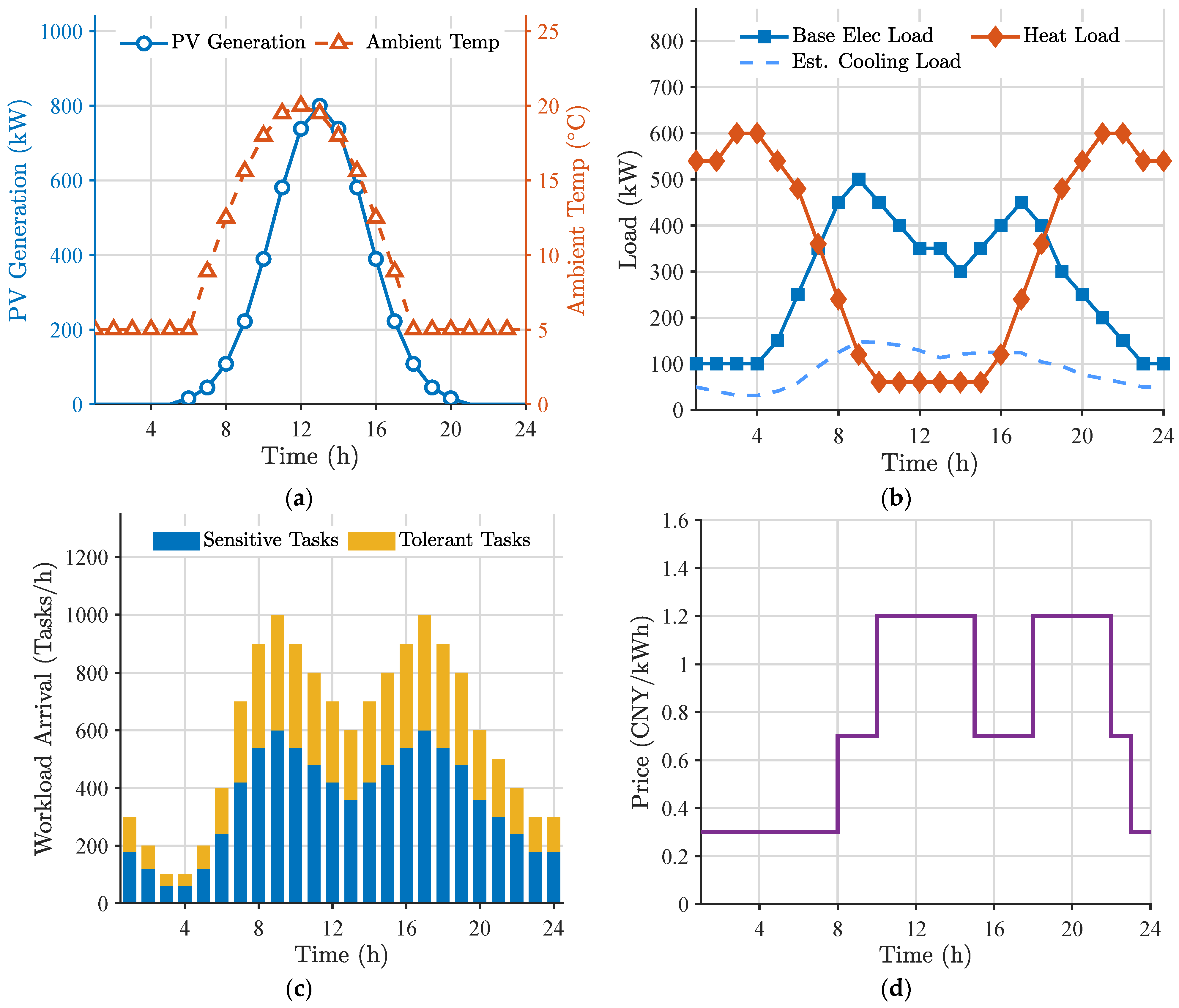
In this study, the typical daily load profile of a campus is adopted to characterize the multiple energy coupling operation environment of the DCMG, as shown in Figure 3. Specifically, Figure 3a depicts the diurnal PV generation and the ambient temperature. Evidently, the PV generation peaks around 12:00, exhibiting a strong positive correlation with the ambient temperature curve. However, Figure 3b reveals that an increase in ambient temperature also leads to an increase in the DC’s cooling energy consumption. Consequently, the superposition of the BEL and the cooling load on this typical day makes the overall electricity demand higher throughout the day. Conversely, the heat load in Figure 3b peaks at night, and it has a complementary characteristic with the power load at this time. Figure 3c illustrates the arrival process of the workload, where tolerant tasks constitute 40% of the total workload, serving as the key controllable resource for implementing the proposed load transfer in this study. Finally, a significant price spread (0.3–1.2 CNY/kWh) is established via the TOU tariff as depicted in Figure 3d, providing economic incentives for energy storage arbitrage and workload scheduling optimization.

To evaluate the performance of different scheduling strategies, four comparative scenarios are established, as outlined in

Table 2. Configuration of comparative scenarios.

Scenario	Workload Shifting	Waste Heat Recovery	Description
Case 1	-	-	Baseline: Basic operation under carbon trading mechanism without active optimization.
Case 2	✓	-	Optimization with flexible workload shifting only.
Case 3	-	✓	Optimization with waste heat recovery only.
Case 4	✓	✓	Proposed: Joint optimization of computing, energy, and carbon.

Note: The carbon trading mechanism is considered in all scenarios. The symbol “✓” indicates that the corresponding strategy is implemented, while “-” indicates it is not.

. Case 1 serves as the baseline scenario, which excludes both workload shifting and WHR, and participates in carbon trading passively (i.e., calculating the carbon cost without optimization measures). Case 2 introduces workload shifting but does not consider the WHR. Case 3 enables WHR but does not implement the workload shifting. Finally, Case 4 integrates the full collaborative strategy proposed in this study. Apart from the different strategy settings, the equipment capacity and external environmental conditions of the four scenarios remain identical.

4.2. Analysis of Multiple Energy Flow Coordination Mechanism

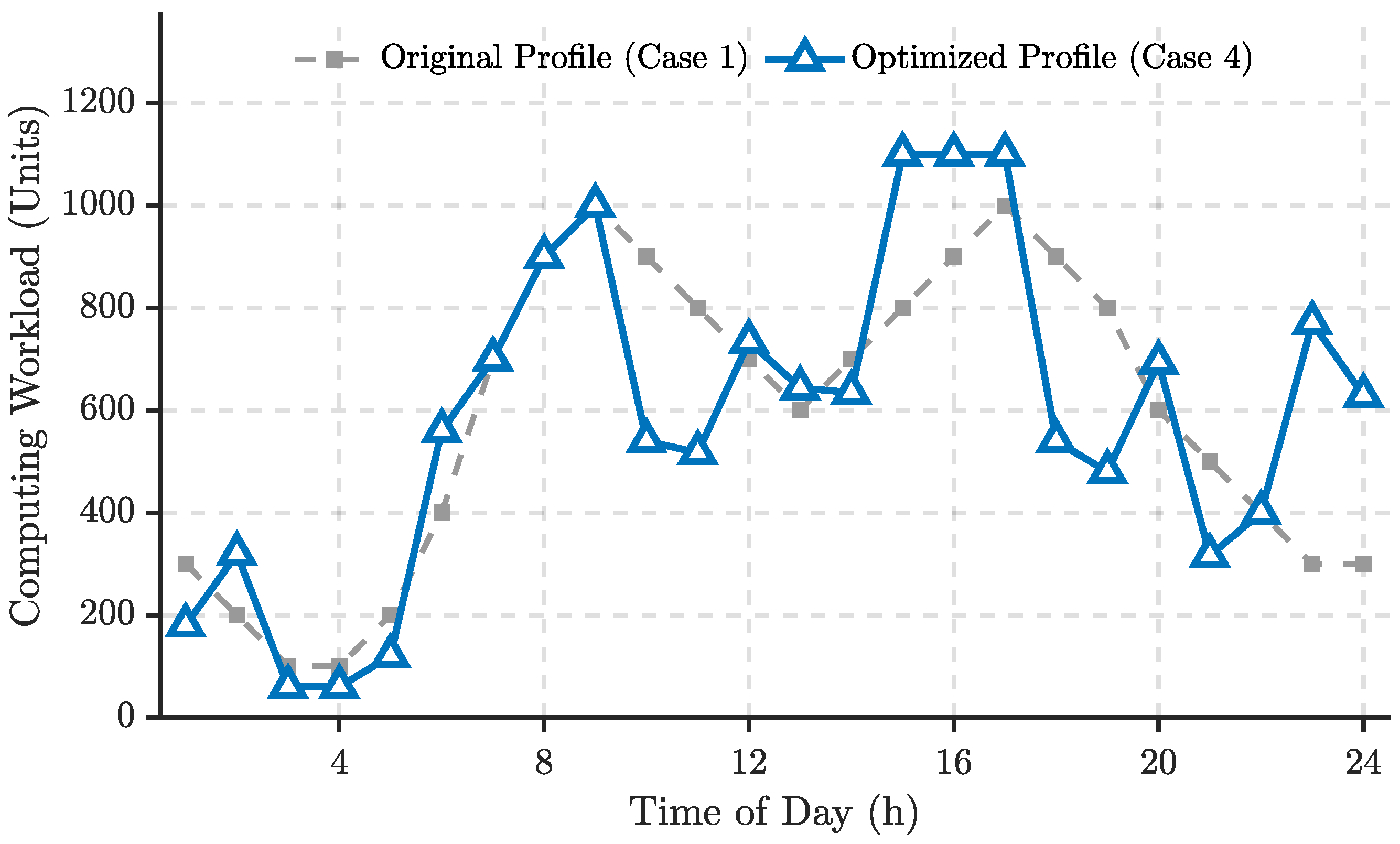
As illustrated in Figure 4, unlike the passive load-following mode in Case 1, Case 4 dynamically adjusts the computing load based on the time-varying electricity prices shown in Figure 3d. Specifically, to minimize operational costs, the system proactively reduces the computing load during peak price periods (10:00–15:00 and 18:00–21:00). Conversely, the accumulated delay-tolerant tasks are concentrated and processed during the flat and valley price periods (15:00–17:00 and after 22:00). This shifting strategy exploits low-cost electricity and provides a cost-effective heat source for WHR to satisfy the nighttime thermal demand.

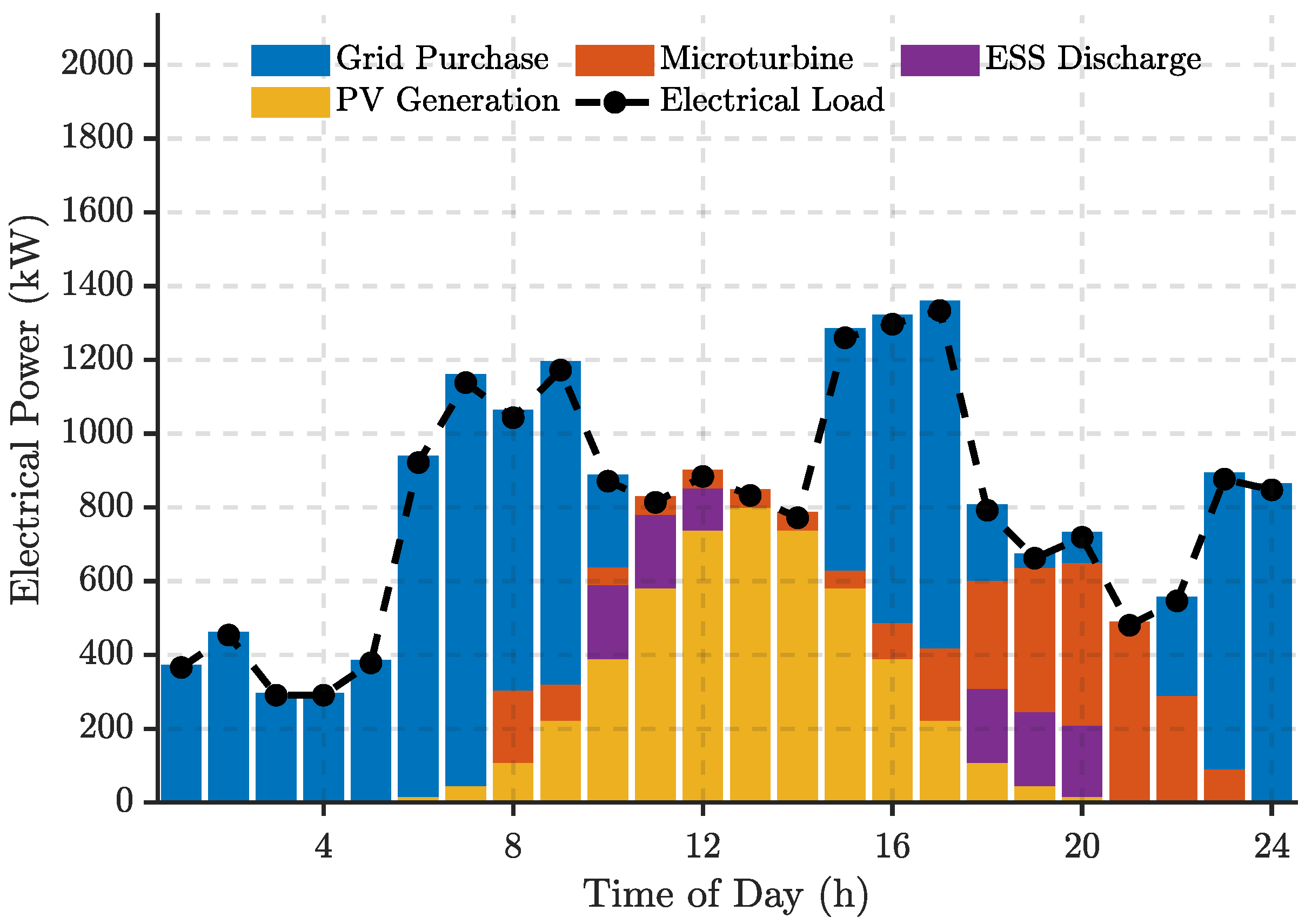
To validate the power allocation characteristics under the multiple energy complementary mechanism, Figure 5 illustrates the electrical energy scheduling strategy in Case 4. During the daytime (10:00–15:00), the system’s energy supply is dominated by PV generation. In contrast, during the evening, as PV output diminishes and electricity prices surge, the MT ramps up its output to support the electrical load in coordination with the ESS. This dispatch mode not only mitigates high electricity purchasing costs but also effectively responds to the surging load demand at night (as shown in Figure 3b). These results demonstrate that the coupled electro-thermal dispatch efficiently realizes energy cascading utilization, thereby significantly reducing basic operating costs while enhancing the system’s balancing capability.

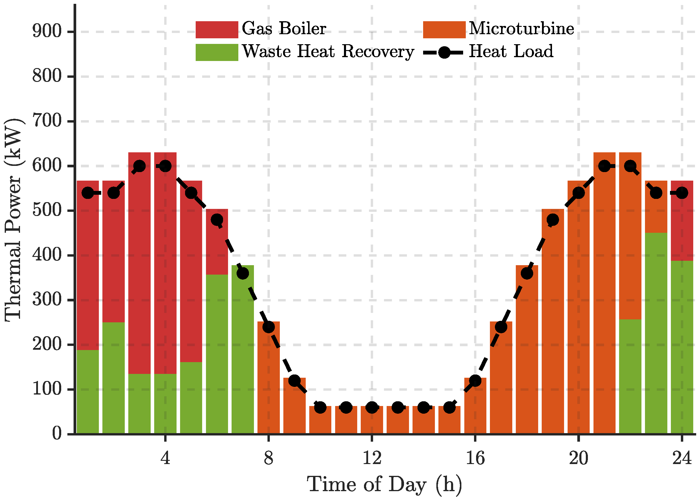
Figure 6 details the thermal scheduling strategy in Case 4. Driven by the workload shifting strategy shown in Figure 4, the system generates substantial waste heat during cold nights to meet the high thermal load. Consequently, the WHR from the DC increases significantly during 00:00–07:00 and 22:00–24:00, thereby displacing the output of the carbon-intensive GB. Entering the evening peak pricing period (18:00–22:00), the MT takes over as the dominant heat source. The MT is dispatched primarily to respond to high electricity prices, and its high-temperature byproduct heat satisfies most of the heating gap. During the daytime (10:00–16:00), the thermal demand is mainly sustained by the MT’s low-level output. This strategy enhances the system’s energy utilization efficiency while guaranteeing thermal supply security.

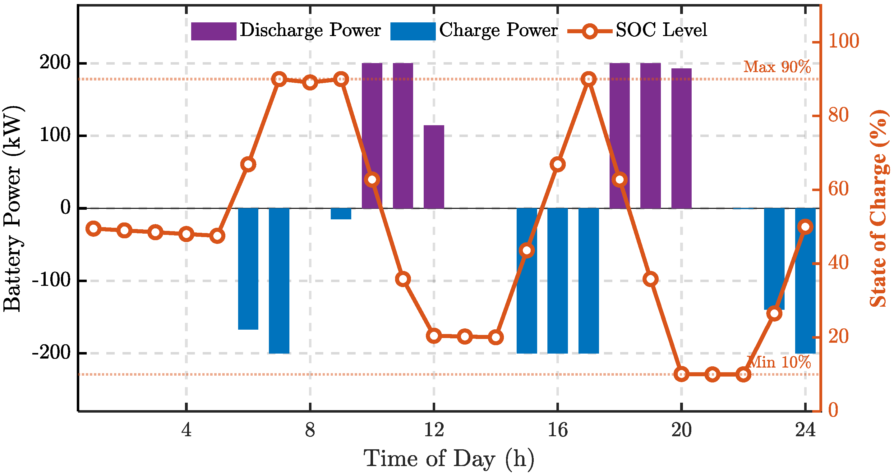
To evaluate the dynamic regulation performance of the ESS under the proposed strategy, Figure 7 illustrates the charging/discharging profiles and SOC variations over a 24 h cycle. As observed, the ESS rapidly charges to 90% during low-electricity-price intervals (06:00–07:00 and 15:00–17:00) and subsequently performs deep discharging during high-price and peak-load periods (10:00–12:00 and 18:00–20:00). By shifting energy from low-cost to high-cost windows, this operational pattern effectively supports computing load demands. In addition, the results demonstrate that the proposed strategy maintains the ESS within safe operating limits (10–90%), which not only enhances net load stability but also strikes a balance between economic efficiency and scheduling flexibility.

4.3. Comparative of Analysis of Economic and Environmental Benefits

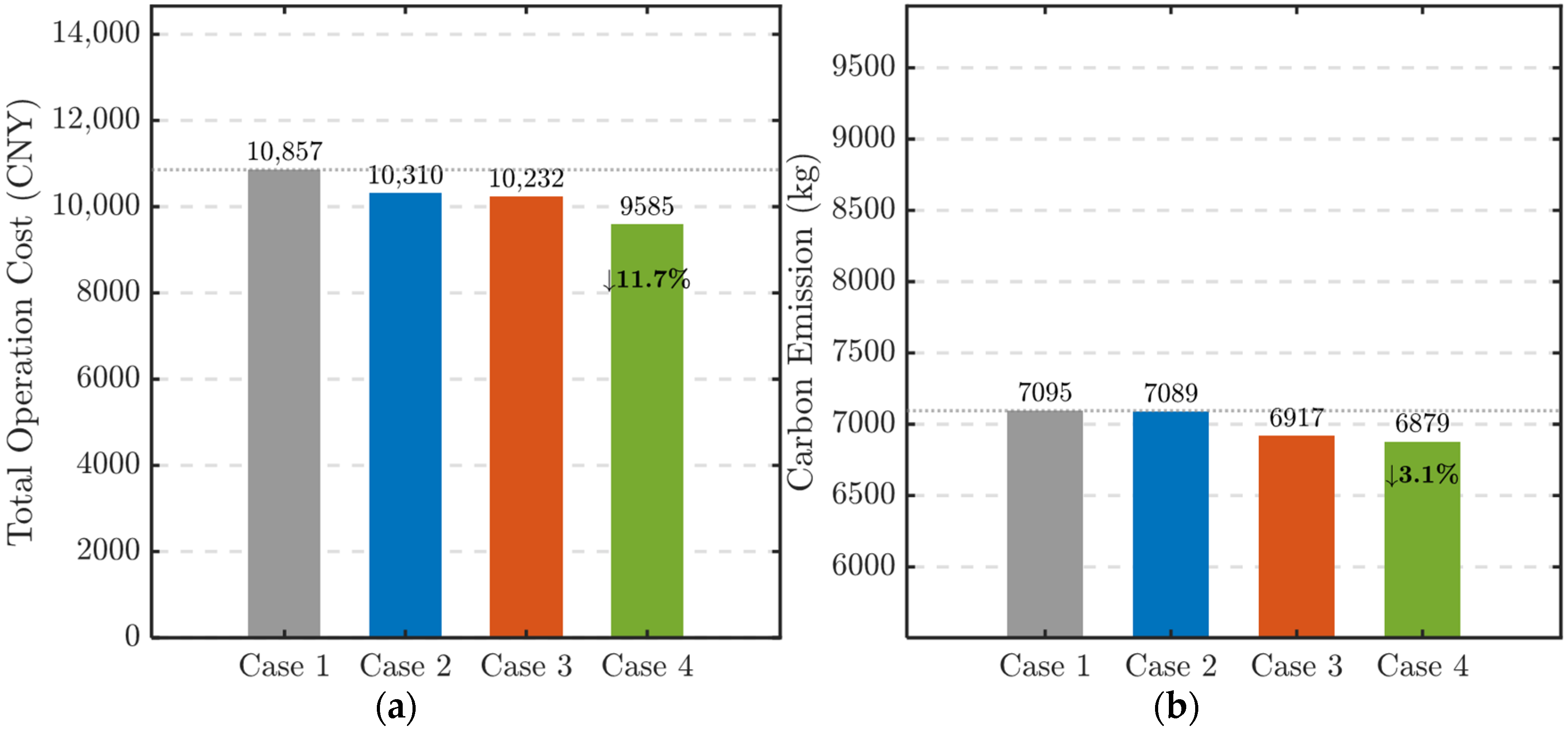
Regarding economic performance, the collaborative optimization strategy (Case 4) exhibited the best results. As shown in Figure 8a, the total operating cost decreased to 9585 CNY, representing an 11.7% reduction compared to the benchmark scenario (Case 1). Notably, this decrease significantly exceeded the simple linear superposition of the effects produced by workload shifting alone (Case 2) or WHR alone (Case 3). This nonlinear gain is attributed to the deep coupling of multiple dimensional resources: the system can synchronously mobilize the flexibility of the computing load and the throughput capacity of the ESS so as to maximize the arbitrage space brought by the peak-valley price difference.

In terms of environmental impact, Case 4 also showed the best performance, with the lowest carbon emissions (6879 kg) in each scenario as illustrated in Figure 8b. This result indicates that the proposed strategy successfully breaks the common trade-off between economy and environmental protection and effectively reduces the carbon footprint of the system while achieving superior cost control. This means that the strategy can achieve dual optimization of economic and environmental benefits under the current price and emission system.

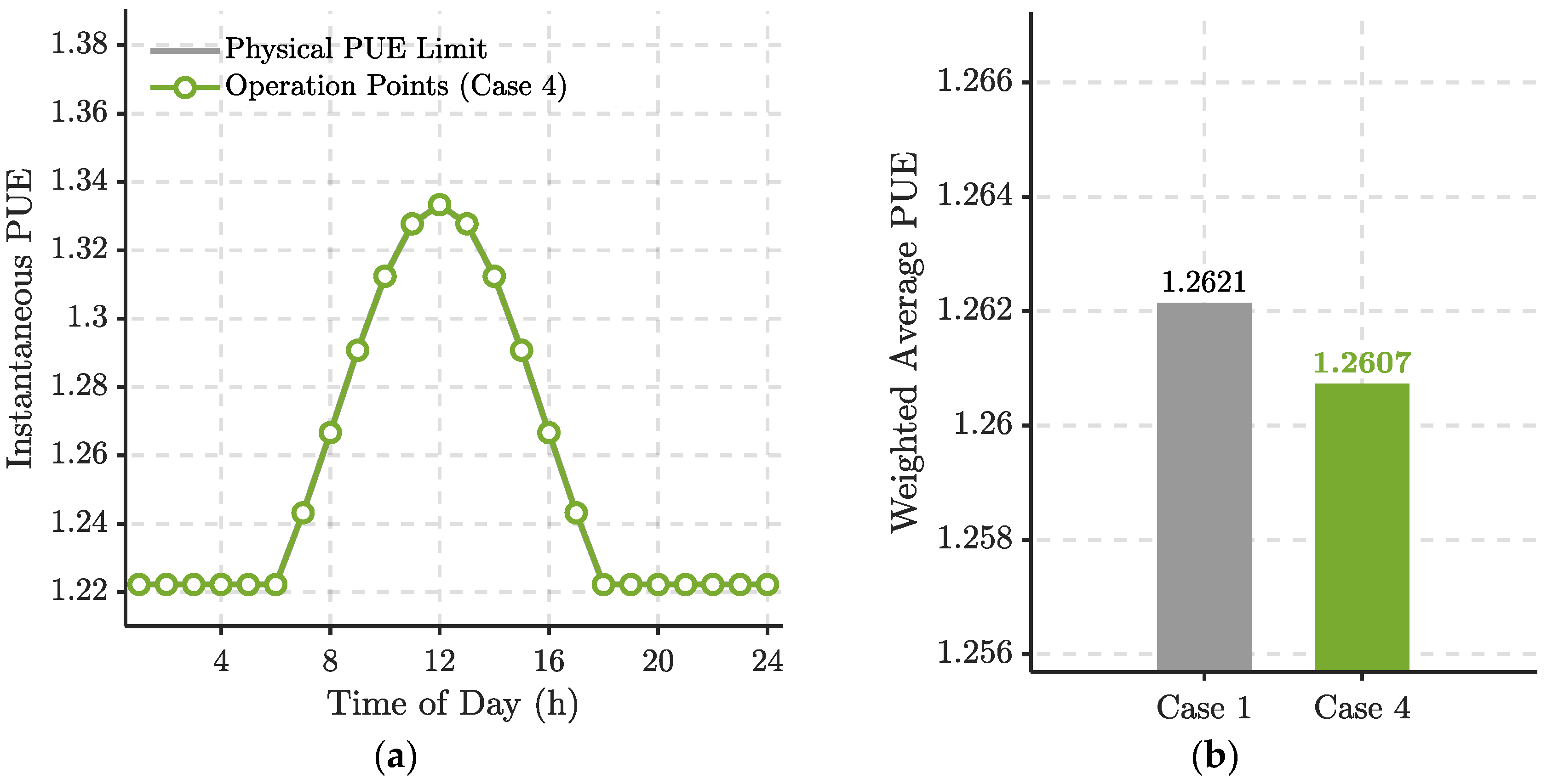
To quantify the energy efficiency performance at the physical level, a dynamic PUE metric is introduced as shown in Figure 9. Distinct from constant PUE models, actual operation demonstrates significant sensitivity to ambient temperature, where PUE values fluctuate markedly between 1.22 and 1.33 (Figure 9a). Leveraging this physical characteristic, the optimization strategy establishes a temperature-aware mechanism that proactively shifts flexible computing loads from high-temperature (high PUE) daytime intervals to cooler nighttime periods. This temporal alignment effectively lowers the cooling overhead per unit of computing load, optimizing the daily weighted average PUE in Case 4 to 1.2607, compared to 1.2621 in the benchmark scenario (Figure 9b). Even though the number change seems small, it is a real improvement in cooling efficiency that was achieved without changing any hardware. For a facility with the 550 kW peak capacity specified in Table 1, this 0.11% improvement translates to a cumulative daily cooling energy saving of approximately 11.1–18.5 kWh. In hyper-scale DC deployments, such software-defined “zero-cost” efficiency gains are highly significant, as they enable the system to fully exploit its operational efficiency potential, thus negating the need for the substantial capital expenditures (typically tens of millions of CNY) usually associated with hardware retrofits.

Table 3. Comparison of economic and environmental performance among scenarios.

Performance Index	Case 1 (Baseline)	Case 2	Case 3	Case 4 (Proposed)	Improvement (vs. Case 1)
Total Operation Cost (CNY)	10,857	10,310	10,232	9585	11.7%
Total Carbon Emission (kg)	7095	7089	6917	6879	3.0%
Average PUE	1.2621	-	-	1.2607	0.11%

summarizes the quantitative improvements in economic cost, carbon emissions, and average PUE across the four scenarios. It is evident that Case 4 achieves the optimal balance among all performance indices.

4.4. Sensitivity and Robustness Analysis

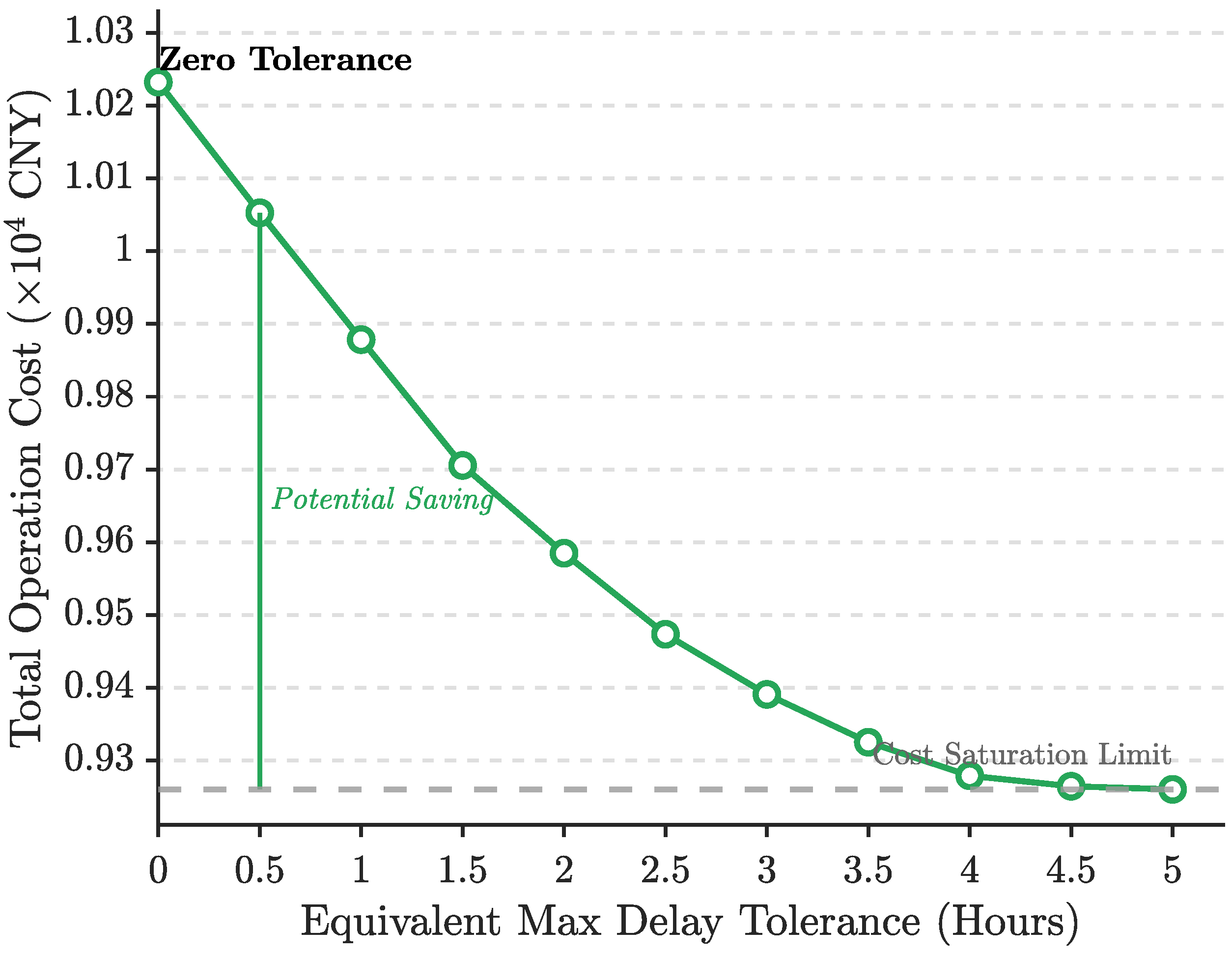
To evaluate the impact of load flexibility on economic performance, Figure 10 shows the operating cost under different maximum delay-tolerances ($D_{max}$). The results show a clear trend of diminishing returns: In the initial stage (0–2.5 h), the cost drops significantly. This indicates that allowing even a short delay enables the system to avoid peak electricity prices, leading to rapid cost savings. However, as the delay-tolerance increases further (especially beyond 4 h), the cost stabilizes near a saturation limit. This is because once the load has been shifted to periods of high PV generation or low electricity prices, extending the delay-time offers no further benefit due to physical constraints such as battery capacity. Therefore, the data suggests that a delay range of 2–3 h is the optimal balance between cost efficiency and service timeliness.

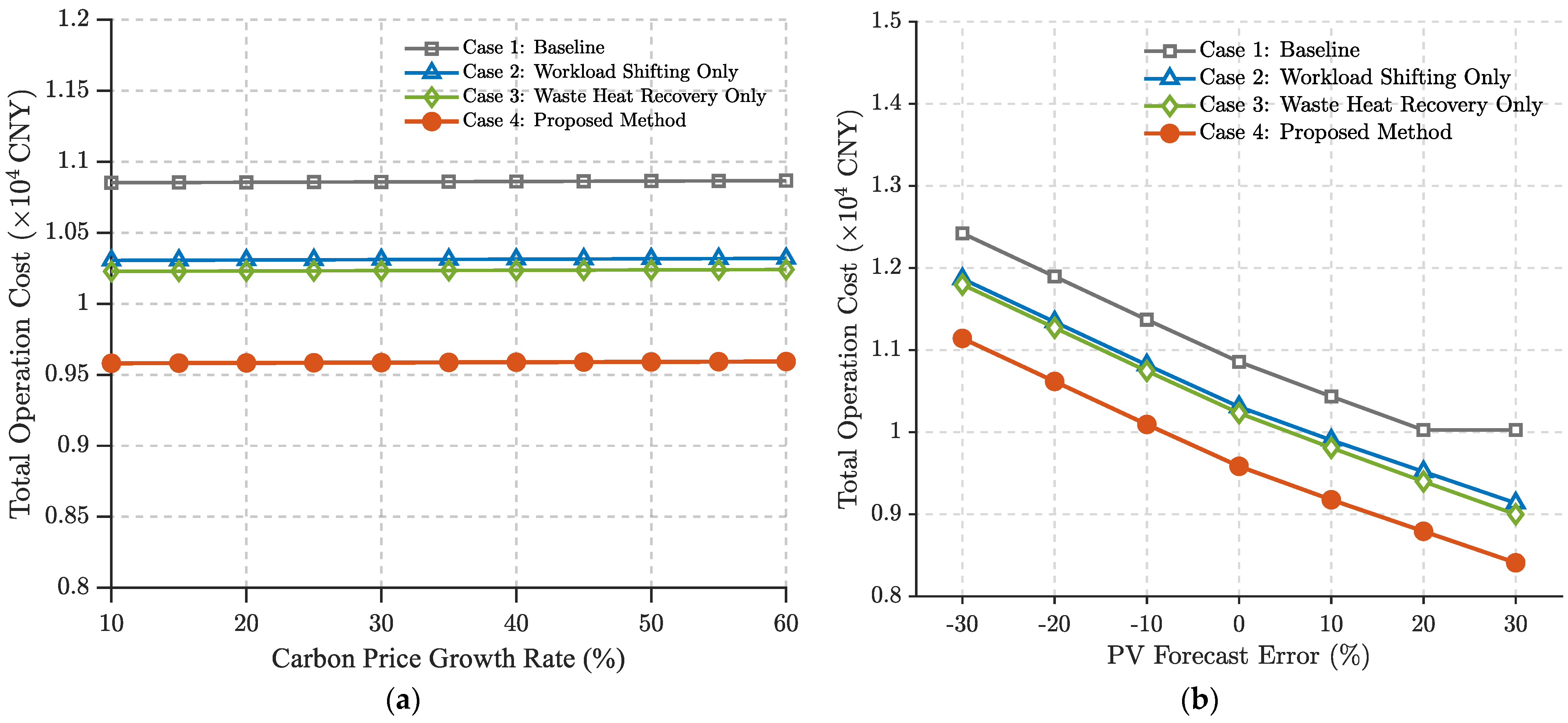
To further verify the stability of these findings, the sensitivity of the total operational cost to economic and environmental uncertainties-specifically carbon price growth rates and PV forecast errors-was investigated. As illustrated in Figure 11a, the economic ranking of the four scenarios (Case 1 > Case 2 > Case 3 > Case 4) remains strictly consistent across a wide range of carbon price growth rates (10% to 60%). This stability confirms that the proposed collaborative strategy provides persistent economic benefits regardless of varying carbon market intensities. Furthermore, Figure 11b depicts the impact of PV forecast errors from −30% to +30%. While absolute costs fluctuate with renewable availability, Case 4 consistently achieves the lowest cost profile even under significant generation deficits. This demonstrates that the “heat-determined computing” mechanism is robust against the inherent stochasticity of source-side energy supply, ensuring reliable performance in practical deployment.

5. Discussion

The results presented in this study rely on specific modeling assumptions to maintain the computational tractability of the MILP framework. Primarily, the server power consumption is modeled as a linear function of CPU utilization, and the thermodynamic model adopts a simplified ambient-temperature-based approach. Additionally, the microgrid model focuses on power-heat balance, omitting distribution network constraints (e.g., voltage limits) and frequent device start-up costs. We acknowledge that in practical engineering, factors such as humidity, airflow organization, and specific cooling architectures significantly impact the actual PUE. However, neglecting these complex nonlinear dynamics and assuming deterministic carbon pricing parameters is a deliberate trade-off to preserve the convexity of the optimization problem, ensuring that the global optimal schedule can be solved efficiently. Consequently, we acknowledge that these simplifications may lead to a slight overestimation of the synergistic economic benefits compared to highly nonlinear real-world operations. These approximations serve as a theoretical baseline, capturing the primary energy flow characteristics for day-ahead scheduling. It is also worth noting that in real-world scenarios, physical factors such as thermal inertia, control latency, and workload heterogeneity may lead to slight deviations from the theoretical hour-level schedule. While these sub-hourly dynamics do not later the general economic trends, they suggest the need for real-time feedback control in actual deployment.

Breaking the limitation of conventional electro-thermal demand response (where typical cost savings range from 3.7% to 12.7% in similar integrated energy dispatch studies [16,27]), the proposed strategy expands the optimization boundary to include computing loads, achieving a significant 11.7% cost reduction (9585 CNY). This significant improvement verifies that extending the control scope from “energy equipment only” to “source–load coordination” unlocks superior efficiency. Such gains originate from the “heat-determined computing” mechanism: by aligning delay-tolerant workloads with thermal demand [22], the system transforms the DC from a passive consumer into a controllable heat source [10,20], thereby maximizing waste heat utility under the tiered carbon trading scheme [32].

Implementing this strategy in real- world scenarios require specific infrastructure conditions. The strategy is specifically designed for delay-tolerant batch workloads (e.g., AI training, data backup) where service level objectives (SLOs) allow hour-level shifting. While task migration introduces minor network overheads, these are outweighed by the significant cooling energy saving in the proposed coarse-grained scheduling. From an implementation perspective, this requires a hierarchical control architecture integrating DC infrastructure management (DCIM) and energy management system (EMS). Standardized interfaces (e.g., Modbus, RESTful APIs) are essential to enable bidirectional communication between the IT scheduling layer (e.g., Kubernetes) and the OT energy control layer (e.g., PLC or SCADA).

The current case study relies on deterministic forecasts. In practice, long-term seasonal variations and stochastic disturbances (e.g., PV intermittency, unexpected workload surges) are inevitable. Although the sensitivity analysis in Section 4.4 demonstrates that the proposed strategy maintains economic advantages under forecast errors of $\pm 30\%$, extreme uncertainties may still cause real-time deviations. Future research will address this by incorporating two-stage robust optimization or stochastic programming to enhance system reliability. Additionally, subsequent work will explore distributed optimization algorithms (e.g., ADMM) to address privacy and scalability issues in geographically dispersed DC networks.

6. Conclusions

This study proposes a low-carbon economic dispatch strategy that integrates the temporal and spatial flexibility of computing power and the cascade utilization of waste heat to address the dual challenges of high energy consumption and carbon emissions faced by DCMG. By constructing a deep coupling framework of bit flow, watt flow, and heat flow and conducting multiple scenario simulation verification, the main conclusions are as follows:

• By quantifying the time shifting potential of delay-tolerant tasks, the strategy can actively shift about 40% of the delayable load from the daytime peak electricity price to the night. This spatiotemporal alignment capitalizes on the lower nocturnal ambient temperatures to reduce cooling energy consumption, successfully optimizing the daily weighted PUE to 1.2607 and validating the energy-saving potential at the physical level.
• The coupling effect between computing power scheduling and WHR is verified by the simulation results. The proposed mechanism effectively transforms the low-grade waste heat from nighttime computing loads into a valuable heating resource. This meets most of the heat load demand. Compared with the traditional mode, this strategy reduces the total operating cost by 11.7%, while minimizing carbon emissions (6879 kg), effectively resolving the trade-off between economic efficiency and environmental protection.
• The sensitivity analysis confirms that a task delay-tolerance of 2–3 h represents the optimal inflection point to balance economic benefits and service timeliness. The results indicate that extending the delay-tolerance beyond this range yields diminishing marginal returns due to the physical capacity constraints of the system.

References

1. Zhuo, Z.; Du, E.; Zhang, N.; Nielsen, C.P.; Lu, X.; Xiao, J.; Wu, J.; Kang, C. Cost increase in the electricity supply to achieve carbon neutrality in China. Nat. Commun. 2022, 13, 3172. [Google Scholar] [CrossRef]
2. Masanet, E.; Shehabi, A.; Lei, N.; Smith, S.; Koomey, J. Recalibrating global data center energy-use estimates. Science 2020, 367, 984–986. [Google Scholar] [CrossRef]
3. Hu, Y.; Zou, K.; Chen, X. The Alchemy of Digital Transformation: How Computing Power Investment Fuels New Quality Productivity. J. Theor. Appl. Electron. Commer. Res. 2025, 20, 354. [Google Scholar] [CrossRef]
4. International Energy Agency (IEA). Electricity 2024: Analysis and Forecast to 2026; IEA: Paris, France, 2024; Available online: https://www.iea.org/reports/electricity-2024 (accessed on 25 January 2026).
5. Hao, Y.; Zhou, H.; Tian, T.; Zhang, W.; Zhou, X.; Shen, Q.; Wu, T.; Li, J. Data centers waste heat recovery technologies: Review and evaluation. Appl. Energy 2025, 384, 125489. [Google Scholar] [CrossRef]
6. de Vries, A. The Growing Energy Footprint of Artificial Intelligence. Joule 2023, 7, 2191–2194. [Google Scholar] [CrossRef]
7. Capozzoli, A.; Primiceri, G. Cooling systems in data centers: State of art and emerging technologies. Energy Procedia 2015, 83, 484–493. [Google Scholar] [CrossRef]
8. Alkrush, A.A.; Salem, M.S.; Abdelrehim, O.; Hegazi, A.A. Data centers cooling: A critical review of techniques, challenges, and energy saving solutions. Int. J. Refrig. 2024, 160, 246–262. [Google Scholar] [CrossRef]
9. Aresti, L.; Panayiotou, G. Applications and new technologies pertaining to waste heat recovery: A vision article. Energies 2025, 18, 2086. [Google Scholar] [CrossRef]
10. Huang, P.; Copertaro, B.; Zhang, X.; Shen, J.; Löfgren, I.; Rönnelid, M.; Fahlen, J.; Andersson, D.; Svanfeldt, M. A review of data centers as prosumers in district energy systems: Renewable energy integration and waste heat reuse for district heating. Appl. Energy 2020, 258, 114109. [Google Scholar] [CrossRef]
11. Oh, J.; Han, U.; Jung, Y.; Kang, Y.T.; Lee, H. Advancing waste heat potential assessment for net-zero emissions: A review of demand-based thermal energy systems. Renew. Sustain. Energy Rev. 2024, 202, 114693. [Google Scholar] [CrossRef]
12. Li, C.; Zheng, K.; Guo, H.; Kang, C.; Chen, Q. Computation-power coupled modeling for IDCs and collaborative optimization in ADNs. IEEE Trans. Smart Grid 2024, 15, 2762–2775. [Google Scholar] [CrossRef]
13. Lyu, X.; Liu, T.; Liu, X.; He, C.; Nan, L.; Zeng, H. Low-carbon robust economic dispatch of park-level integrated energy system considering price-based demand response and vehicle-to-grid. Energy 2023, 263, 125739. [Google Scholar] [CrossRef]
14. He, Y.; Zhang, Y. Optimal configuration of shared energy storage for multi-microgrid systems: Integrating battery decommissioning value and renewable energy economic consumption. Energy Convers. Manag. 2025, 343, 120156. [Google Scholar] [CrossRef]
15. Wang, L.; Xian, R.; Jiao, P.; Chen, J.; Chen, Y.; Liu, H. Multi-timescale optimization of integrated energy system with diversified utilization of hydrogen energy under the coupling of green certificate and carbon trading. Renew. Energy 2024, 228, 120597. [Google Scholar] [CrossRef]
16. Hao, X.; Liu, P.; Deng, Y. Joint optimization of operational cost and carbon emission in multiple data center micro-grids. Front. Energy Res. 2024, 12, 1344837. [Google Scholar] [CrossRef]
17. Li, H.; Li, X.; Chen, S.; Li, S.; Kang, Y.; Ma, X. Low-carbon optimal scheduling of integrated energy system considering multiple uncertainties and electricity-heat integrated demand response. Energies 2024, 17, 245. [Google Scholar] [CrossRef]
18. Wang, R.; Wen, X.; Wang, X.; Fu, Y.; Zhang, Y. Low carbon optimal operation of integrated energy system based on carbon capture technology, LCA carbon emissions and ladder-type carbon trading. Appl. Energy 2022, 311, 118664. [Google Scholar] [CrossRef]
19. Pakere, I.; Blumberga, D.; Volkova, A.; Lepiksaar, K.; Zirne, A. Valorisation of waste heat in existing and future district heating systems. Energies 2023, 16, 6796. [Google Scholar] [CrossRef]
20. Yuan, X.; Liang, Y.; Hu, X.; Xu, Y.; Chen, Y.; Kosonen, R. Waste heat recoveries in data centers: A review. Renew. Sustain. Energy Rev. 2023, 188, 113777. [Google Scholar] [CrossRef]
21. Xia, B.; Kong, F.; Zhou, J.; Tang, X.; Gong, H. A delay-tolerant data transmission scheme for internet of vehicles based on software defined cloud-fog networks. IEEE Access 2020, 8, 65911–65922. [Google Scholar] [CrossRef]
22. Zhu, L.; Wu, S.; Liu, H.; Wang, Q.; Tang, Y. Spatio-temporal load migration potential of data centers: Evaluation and application. Front. Energy Res. 2023, 11, 1289275. [Google Scholar] [CrossRef]
23. Ebrahimi, K.; Jones, G.F.; Fleischer, A.S. A review of data center cooling technology, operating conditions and the corresponding low-grade waste heat recovery opportunities. Renew. Sustain. Energy Rev. 2014, 31, 622–638. [Google Scholar] [CrossRef]
24. Oró, E.; Depoorter, V.; Garcia, A.; Salom, J. Energy efficiency and renewable energy integration in data centres: Strategies and modelling review. Renew. Sustain. Energy Rev. 2015, 42, 429–445. [Google Scholar] [CrossRef]
25. Yin, X.; Ye, C.; Ding, Y.; Song, Y. Exploiting internet data centers as energy prosumers in integrated electricity-heat system. IEEE Trans. Smart Grid 2023, 14, 167–182. [Google Scholar] [CrossRef]
26. Socci, L.; Rocchetti, A.; Verzino, A.; Zini, A.; Talluri, L. Enhancing third-generation district heating networks with data centre waste heat recovery: Analysis of a case study in Italy. Energy 2024, 313, 134013. [Google Scholar] [CrossRef]
27. Wang, Y.; Ma, Y.; Song, F.; Ma, Y.; Qi, C.; Huang, F.; Xing, J.; Zhang, F. Economic and efficient multi-objective operation optimization of integrated energy system considering electro-thermal demand response. Energy 2020, 205, 118022. [Google Scholar] [CrossRef]
28. Pan, D.; Zhang, L.; Wang, B.; Jia, J.; Song, Z.; Zhang, X. Multi-objective planning of integrated energy system based on CVaR under carbon trading mechanism. Front. Energy Res. 2024, 12, 1310301. [Google Scholar] [CrossRef]
29. Yang, Y.; Zhang, J.; Chen, T.; Yan, H. Low-carbon optimization of integrated energy systems with time-of-use carbon metering on the user side. Energies 2024, 17, 2071. [Google Scholar] [CrossRef]
30. Cheng, Y.; Zhang, N.; Lu, Z.; Kang, C. Modeling carbon emission flow in multiple energy systems. IEEE Trans. Smart Grid 2019, 10, 3562–3574. [Google Scholar] [CrossRef]
31. Fagundes, T.A.; Fuzato, G.H.F.; Silva, L.J.R.; dos Santos Alonso, A.M.; Vasquez, J.C.; Guerrero, J.M. Battery Energy Storage Systems in Microgrids: A Review of SoC Balancing and Perspectives. IEEE Open J. Ind. Electron. Soc. 2024, 5, 961–992. [Google Scholar] [CrossRef]
32. Shi, L.; Liang, C.; Zhou, J.; Li, Y.; Liu, J.; Wu, F. Optimal scheduling of integrated energy systems with a ladder-type carbon trading mechanism and demand response. Front. Energy Res. 2024, 12, 1363285. [Google Scholar] [CrossRef]
Figure 1. Schematic Diagram of the DCMG.
Energies 19 00699 g001
Figure 2. Hierarchical Scheduling Framework for the DCMG.
Energies 19 00699 g002
Figure 3. Typical daily profiles of the DCMG: (a) PV generation and ambient temperature; (b) base electrical and thermal loads; (c) sensitive and tolerant tasks distribution; and (d) TOU electricity tariff.
Energies 19 00699 g003
Figure 4. Comparison of computing workload profiles: Passive operation (Case 1) vs. Proposed optimized scheduling (Case 4).
Energies 19 00699 g004
Figure 5. Electrical power dispatch results and source–load balance analysis under the proposed strategy (Case 4).
Energies 19 00699 g005
Figure 6. Thermal power dispatch results and source–load balancing characteristics under the proposed strategy (Case 4).
Energies 19 00699 g006
Figure 7. Optimal scheduling of the ESS under the proposed cooperative strategy (Case 4): charging/discharging power and SOC evolution.
Energies 19 00699 g007
Figure 8. Comparison of system performance metrics across benchmark scenarios (Case 1–3) and the proposed cooperative strategy (Case 4): (a) Total operational cost; and (b) Carbon emissions.
Energies 19 00699 g008
Figure 9. Analysis of physical energy efficiency: (a) Variation in dynamic PUE with ambient temperature showing operation points from Case 4; and (b) Improvement in weighted average PUE achieved by the proposed strategy compared to Case 1.
Energies 19 00699 g009
Figure 10. Sensitivity analysis of total operational cost of the proposed strategy (Case 4) with respect to maximum delay-tolerance.
Energies 19 00699 g010
Figure 11. Robustness check of total operational cost: (a) Impact of carbon price growth rate; (b) Impact of PV forecast error.
Energies 19 00699 g011