An Optimization Method for Reserve Capacity Operation in Urban Integrated Energy Systems Considering Multiple Uncertainties

Abstract

Urban integrated energy systems (UIESs) are increasingly exposed to uncertainties arising from wind and photovoltaic variability, load fluctuations, and equipment failures, highlighting the need for refined reserve assessment and coordinated operation. This study develops a unified framework that jointly models renewable and load deviations together with a load-dependent failure probability model, using Monte Carlo sampling and K-means scenario reduction to obtain representative system states. A reserve-capacity-oriented optimisation model is formulated to minimise total operating cost—including thermal generation, energy-storage operation, and reserve cost—while satisfying power balance, reserve adequacy, unit operating limits, and state-of-charge constraints. Application to a UIES comprising a 1000 kW load, 800 kW photovoltaic unit, 100 kW wind turbine, five thermal power units (total capacity 1000 kW), and a 250 kW/370 kWh energy storage system shows that reserve requirements fluctuate between −100 kW (downward) and 500 kW (upward) across different scenarios, with uncertainty-driven reserves dominating and failure-related reserves remaining below 100 kW. The optimisation results indicate coordinated operation between thermal units and storage, with storage absorbing surplus renewable output, supporting peak shaving, and providing most upward and all downward reserves. The total operating costs under typical summer and winter scenarios are 2264.02 CNY and 3122.89 CNY, respectively, confirming the method’s ability to improve reserve estimation accuracy and support economical and reliable UIES operation under uncertainty.

1. Introduction

The large-scale integration of renewable energy sources, coupled with the diversification of load profiles, has led to a significant increase in the operational uncertainty of the urban integrated energy system (UIES). In the current context, the demands for system reliability and flexibility have grown correspondingly, thus necessitating the rational allocation of reserve resources to ensure energy supply security [1,2]. Given the aforementioned context, it is imperative that the system optimise the utilization of distributed adjustable resources, thereby fostering regional autonomy and achieving efficient internal energy balance. Reserve capacity is defined as the available generation capacity or regulation capacity reserved to cope with unit failures, sudden load changes, and fluctuations in the reserve capacity of wind and solar output. System reserve configuration has been demonstrated to directly affect the cost of reserves, the system’s overall operational economy, as well as the system’s safe and stable operation under various disturbance scenarios. In the context of UIES, balancing economic efficiency with the mitigation of multiple uncertainties has become a critical issue that demands urgent attention, especially amid the growing renewable energy penetration [3,4]. The present study focuses on the UIES and investigates the optimal operation of reserve capacity under multiple uncertainties, including renewable output variability/intermittency, demand response behavior and equipment failures. The objective of this study is twofold: first, to reduce overall operating costs, and second, to ensure system reliability by means of more rational allocation of reserve resources.

In the study of reserve requirement, early research predominantly adopted simple rules or empirical formulas, such as determining reserve levels according to the maximum reserve capacity of online units. While these methods are intuitive, they demonstrate limited accuracy in structurally complex systems characterised by dynamic operational states [5]. Subsequently, researchers introduced probabilistic statistical methods for estimating reserve requirements. However, the evaluation results remain prone to biases regarding time-varying characteristics and granularity, due to the limitations associated with real-time data and high-quality historical data [6]. In recent years, references [7,8] have adopted non-parametric kernel density estimation to conduct dynamic probabilistic evaluations of ramping and operational reserves. In reference [9], the gate function was incorporated into the Laplace distribution to account for errors in wind power forecasting. The reference [10] improved the accuracy of day-ahead AGC reserve requirement forecasting by integrating Fourier features, attention mechanisms, and an improved whale algorithm. As shown in studies [11,12], the reserve requirement induced by photovoltaic fluctuations was characterized by means of Monte Carlo scenarios and spectral analysis. These efforts have promoted the development of reserve requirement assessment from empirical rules towards probabilistic and data-driven approaches. However, the majority of studies focus solely on single-source uncertainties, and there is a lack of integrated characterization of multi-source uncertainties such as wind and solar output, user behaviour, and equipment failures.

Subsequently, the quantification of reserve capacity has been integrated with uncertainty scenarios and risk metrics. Reference [13] adopts scenario analysis to simulate system uncertainties and develops a reserve capacity acquisition method linked to risk levels via indicators such as Expected Energy Shortfall (EENS) and Energy Waste Risk (EWWR). The reference [14] addresses maintenance uncertainty by proposing a maintenance reserve capacity adequacy metric based on Monte Carlo simulation. The study [15] classifies reserve requirement into imbalance reserves and System Reliability reserves, and provides a reserve requirement quantification method suitable for grids with high wind power penetration. Reference [16] combines Copula theory with distribution-robust optimization to establish a quantification framework for Secondary Frequency Control reserve capacity, while explicitly incorporating frequency security constraints into the reserve allocation process. Studies in this domain have evolved from simple deterministic validation for reserve capacity quantification towards risk-based probabilistic assessment. However, the majority of studies focus on single power systems and standalone System Reliability metrics, resulting in a lack of integrated support for multi-energy coupling, multi-source uncertainties, and operational optimisation in the context of UIES.

Following the characterisation of reserve requirement and reserve capacity levels, the research focus has shifted to the economically efficient allocation of reserve resources and operational optimisation. Conventional approaches historically concentrated on single-generation resources; however, recent studies have placed increasing emphasis on multi-resource coordination and multi-timescale synchronisation. The paper [17] constructs a two-stage robust optimization model that incorporates wind power, reserve requirement and demand response. The article [18] points out that implementing Risk reserve requirements in unit portfolios helps balance costs and risks. In terms of market mechanisms, the reference [11] proposes a reserve cost allocation mechanism based on VCG theory, while the paper [2] designs a bilateral reserve capacity mechanism to enhance wind power integration. The reference [19] classifies reserve types by time scale and employs Fourier transforms to ensure precise quantification. As demonstrated in studies [20,21], the regulatory potential of demand response in reserve systems is explored from the perspective of source-grid-load coordination. This advancement in reserve optimisation represents a shift from a single generation-side approach to a new paradigm of “source-grid-load-storage” coordinated dispatch. However, most extant studies in this field focus primarily on power systems, indirectly treating uncertainties as exogenous scenarios or demand inputs. In the context of UIES, insufficient attention has been paid to the tight coupling between the modelling of reserve requirement (driven by multi-source uncertainties such as wind and solar output, user response, and equipment failures) and operational optimisation.

In summary, while existing research has advanced the quantification of reserve requirement, risk assessment, and multi-resource coordination, gaps still exist in multi-factor joint modelling, coordinated optimisation under complex systems, and engineering feasibility. To address the multiple uncertainties inherent in the UIES—such as fluctuating renewable generation, demand response behaviour, and equipment failures—this paper proposes a reserve capacity operation optimisation method. The following contributions are of particular significance:

• This paper focuses on the Integrated Modelling of Multi-Source Uncertainty. Integrating three types of uncertainties—wind and solar output variability, user response, and equipment failure—into a unified framework constitutes a key objective. Monte Carlo scenario sampling is adopted to characterize random fluctuations in wind and solar power. Price elasticity and multi-energy coupling are incorporated to describe user response behaviour. Furthermore, a load-based Piecewise Failure Probability Model is utilized to represent equipment operational risks. This approach helps improve both the authenticity and comprehensiveness of reserve requirement characterization at its source.
• Probabilistic and Refined Reserve Capacity Optimization Model: This paper proposes an operational optimization model oriented to reserve capacity, with the objective of minimizing the sum of generation costs and reserve costs. This model integrates power balance, reserve adequacy, unit operating constraints, and engineering conditions. The latter include ESS Charging/Discharging Constraints and State-of-Charge (SOC) Constraints. Its primary function is to realize joint constraint and risk measurement for wind/solar fluctuations, response uncertainties, and failure risks. This model is designed to achieve the coordinated allocation of reserve resources, balancing system reliability and economy.
• This paper explores the potential of enhanced solution strategies for high-dimensional nonlinear problems and proposes the improved firefly algorithm as the solution tool. Adaptive step size adjustment, automatic population splitting, and constraint handling mechanisms are integrated to enhance the algorithm’s global search capability and convergence stability. This effectively addresses the model’s characteristics of high dimensionality, multiple constraints, and non-convexity, thereby offering a scalable and robust suboptimal solution approach for reserve capacity operation optimization at the UIES scale.

2. Quantification Model for Reserve Requirement Considering Multi-Source Uncertainty

As the penetration of renewable energy continues to increase and load variability intensifies, the UIES is confronted with multiple uncertainties arising from both the generation and load sides. To ensure system supply, reliability, and operational efficiency, it has become imperative to scientifically quantify reserve requirements in both planning and dispatch processes. This chapter addresses system uncertainties by first modeling the unpredictability of wind and solar power generation as well as load fluctuations, and then establishing a load-factor-considered Equipment Failure Probability model. A methodology for quantifying System reserve requirement is proposed, aiming to integrate multi-source uncertainties. This approach lays the foundation for the subsequent development of optimized dispatch models.

2.1. Quantitative Model for System Source Load Uncertainty

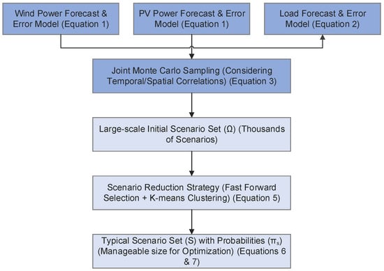
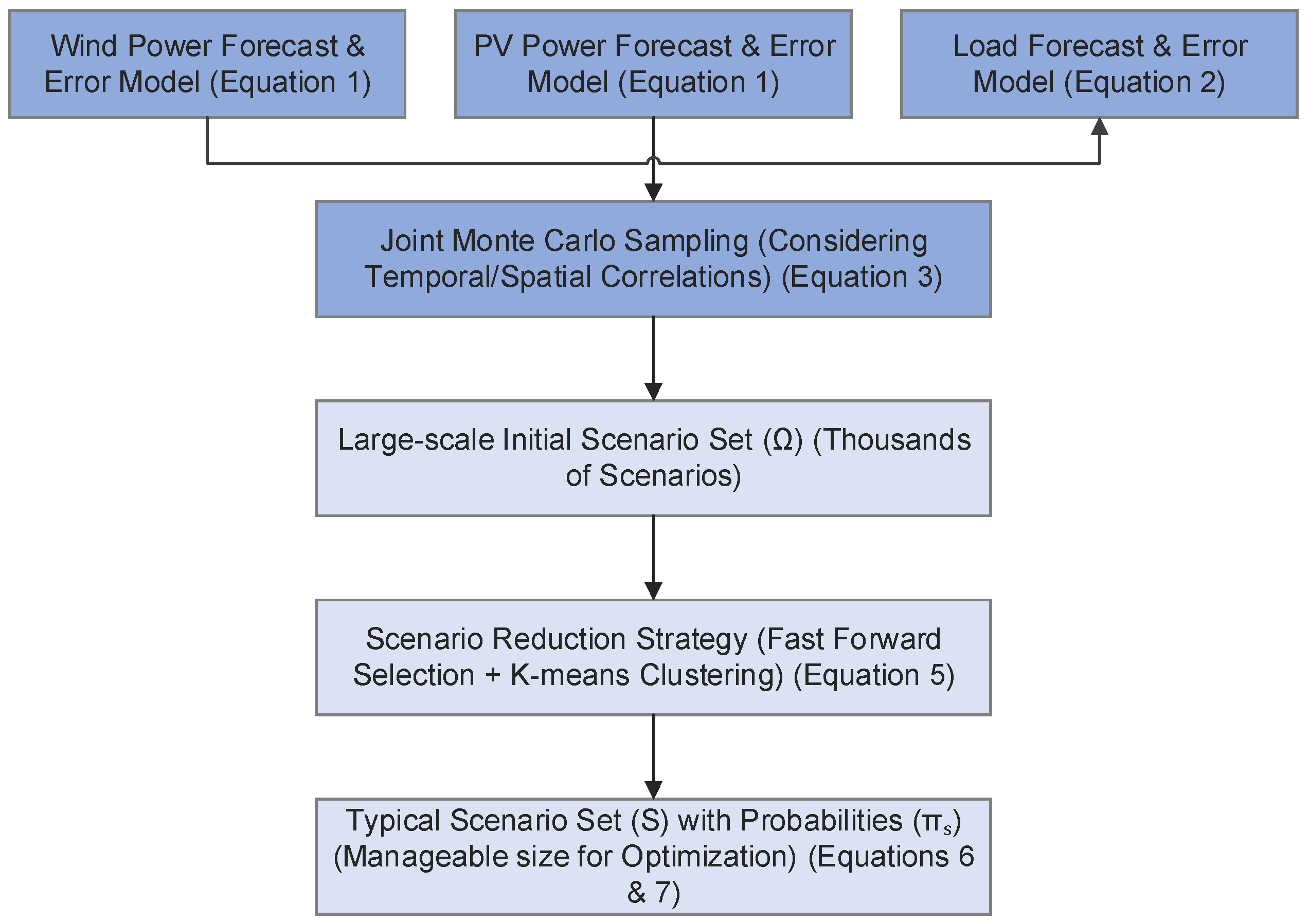
In the UIES, significant uncertainties exist in wind power output, photovoltaic output, and electrical load, with these three components often exhibiting temporal and spatial correlations. To characterize these uncertainties within a unified framework while balancing model accuracy and computational tractability, this paper adopts a “forecast value + random deviation” representation for both renewable generation and load. Using a “Monte Carlo scenario generation + scenario reduction” approach, continuous probability distributions are transformed into a finite set of representative scenarios, as shown in Figure 1. This unified modeling framework enables the simultaneous consideration of uncertainties related to wind and solar fluctuations as well as load-side behavior within a finite scenario set. Based on typical scenarios and their probabilities of occurrence, it becomes feasible to construct multi-scenario optimization solutions for dispatch and planning purposes.

Figure 1. Joint Scenario Generation and Reduction Framework.

2.1.1. Differentiated Characterization of Random Deviation Models

• Wind Power and PV Power Forecasting Error Model

The generation of wind and solar power is directly influenced by meteorological variations, characterized by strong randomness and high-frequency fluctuations. Consequently, the prediction error can be modeled as a normal random variable with a mean of zero.

$$\mathrm{\Delta }{P}_t^W\sim {\rm N}\left(0,{\mathcal{\sigma }}_W^2\right),\mathrm{\Delta }{P}_t^S\sim {\rm N}\left(0,{\mathcal{\sigma }}_S^2\right)$$

(1)

In the formula, $\mathrm{\Delta }{P}_t^W$ and $\mathrm{\Delta }{P}_t^S$ represent the prediction errors for wind power and photovoltaic output at time $t$, respectively; ${\mathcal{\sigma }}_W^2$ and ${\mathcal{\sigma }}_S^2$ denote the variances of the wind power and photovoltaic prediction errors, respectively, which can be obtained from the statistical analysis of wind speed–power and irradiance–power errors.

A comparison of load, wind, and solar power deviations indicates that these deviations mainly originate from meteorological forecast errors, which leads to a relatively stable variance that shows little dependence on power levels.

2.

Load Forecasting Error Model

Load uncertainty is primarily driven by factors including user behavior, meteorological conditions, and industrial activities. The observed fluctuations exhibit clear diurnal periodicity, seasonal patterns, and abrupt variations. As a result, the variance of the load forecasting error demonstrates a correlation with load levels. The following model is adopted in this paper:

$$\mathrm{\Delta }{L}_t\sim N\left(0,\alpha {\widehat{L}}_t\right)$$

(2)

$\mathrm{\Delta }{L}_t$ stands for the Load Forecasting Error at time t; ${\widehat{L}}_t$ denotes the load forecast value at time t; and $\alpha$ is obtained by fitting the residuals between historical forecasts and actual loads.

In contrast to wind and solar power, load deviation exhibits more significant behavioral correlation and temporal autocorrelation characteristics. Although its error distribution is more stable, it varies with the magnitude of the forecasted load. This study models the forecasting errors of wind power, photovoltaic power, and load using a zero-mean normal distribution. This assumption is widely adopted in power system dispatch research and serves as an effective benchmark analysis method [22].

2.1.2. Joint Scenario Generation Method

To preserve the temporal correlation and stochastic coordination characteristics among wind, solar, and load, this paper employs a joint Monte Carlo method based on the aforementioned error models to generate a large-scale initial scenario set.

Through joint sampling from the three random deviation models, the joint temporal trajectories of these three variables can be obtained:

$${\mathrm{\Omega }}^0=\left\{{\omega }_1,{\omega }_2,\dots {\omega }_{N_0}\right\}$$

(3)

In the equation, ${\mathrm{\Omega }}^0$ is the initial scene set; $\omega \in {\mathrm{\Omega }}^0$ denotes a single scene containing complete wind power, photovoltaic, and load trajectories:

$${\left(P_{t,\omega }^W,P_{t,\omega }^S,L_{t,\omega }\right)}_{t=1}^T$$

(4)

$P_{t,\omega }^W$, $P_{t,\omega }^S$ and $L_{t,\omega }$ stand for the output trajectories of wind power, photovoltaic power, and load at time t and scenario ω, respectively; ${\left(P_{t,\omega }^W,P_{t,\omega }^S,L_{t,\omega }\right)}_{t=1}^T$ denotes the joint generation approach, which has been demonstrated to better capture the cooperative fluctuation characteristics observed among wind, solar, and load in real systems compared to scenarios generated separately.

2.1.3. Scenario Reduction and Construction of Typical Scene Sets

Given that the initial number of scenarios typically reaches the thousands, direct incorporation into optimization models would cause a dimensionality explosion. To extract representative typical scenarios from the large-scale initial scenario set (N = 1000) generated by Monte Carlo simulation, scenario reduction techniques are required. Common reduction methods mainly fall into two categories: one is algorithms based on iterative probabilistic distance screening, such as fast forward selection; the other is algorithms based on data similarity clustering analysis, such as K-means clustering. The former selects scenarios by progressively minimizing probabilistic distances, while the latter performs unsupervised grouping according to the morphological features of output curves. This study selects the K-means clustering algorithm as the scenario reduction method, primarily based on the following considerations: First, the optimization model in this study focuses more on the manifestation of source-load uncertainty in terms of typical output curve patterns, and K-means can directly extract cluster centroids that characterize these morphological features. Second, this method demonstrates high computational efficiency and strong stability when handling large-scale initial scenarios. To address this issue, this paper employs the K-means clustering algorithm to reduce the joint scenario set, thereby obtaining a manageable set of representative typical scenarios.

$$\mathrm{\Omega }=\left\{{\omega }_1,{\omega }_2,\dots ,{\omega }_N\right\},N\ll N_0$$

(5)

$\mathrm{\Omega }$ represents the set of typical scenarios; ${\omega }_i$ in the typical scenario set $\mathrm{\Omega }$; $N$ denotes the number of scenarios in the typical scenario set; and $N_0$ indicates the number of scenarios in the initial scenario set. The scenario probability is found to satisfy the following condition:

$${\displaystyle \sum _{i=1}{\pi }_{{\omega }_i}}=1,i=1,2,\dots ,N$$

(6)

${\pi }_{{\omega }_i}$ is set as the probability corresponding to the typical scenario ${\omega }_i$ in the typical scenario set $\mathrm{\Omega }$. Each archetypal scenario contains complete integrated trajectories for wind, solar, and load, which are employed in subsequent scheduling and planning models.

2.1.4. Unified Uncertainty Scenario Characterization Model

The actual quantities of the three uncertain variables in the scenario are expressed as follows:

$$X_{t,{\omega }_i}={\widehat{X}}_t+\mathrm{\Delta }{X}_{t,{\omega }_i},X\in \left\{P^W,P^S,L\right\},i=1,2,\dots ,N$$

(7)

$P^W$ represents wind power capacity; $P^S$ denotes photovoltaic power capacity; $L$ indicates electricity load; $t$ serves as the time index; $i$ denotes the scenario index (corresponding to the typical scenario ${\omega }_i$); ${\widehat{X}}_t$ signifies the forecast/baseline value, indicating the point forecast or expected value of variable $X$ at period $t$, serving as the baseline against which all scenario fluctuations are measured; $\mathrm{\Delta }{X}_{t,{\omega }_i}$ denotes the random deviation, representing the random fluctuation of variable $X$’s actual value relative to its forecast value at period t and scenario ${\omega }_i$. This deviation is derived from statistical analysis of historical errors or probability distributions of each uncertain variable.

2.2. Probability Model for System Risk Considering Equipment Failures

In the context of Integrated Energy Systems (IESs) in industrial parks, the operational status of each energy supply device directly affects the stability and safety of the system’s energy supply. Conventional research methods often assume a static Equipment Failure Probability, neglecting the dynamic interaction between equipment load conditions and failure probability during actual operation. To address this issue, this section establishes a failure probability model based on equipment load factors, thereby providing a more accurate description of operational risks.

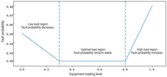
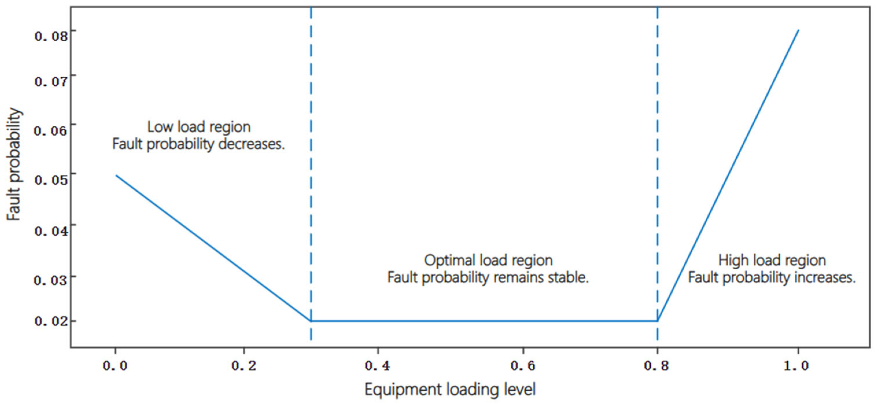
Existing research indicates that the magnitude of equipment load significantly influences failure probability. It has been shown that prolonged heavy-load operation causes internal heat accumulation, which accelerates the aging process. Conversely, prolonged light-load operation intensifies internal vibrations, jitter, and wear, thereby compromising operational safety. Therefore, based on equipment characteristics, the relationship between equipment failure probability and load rate is categorized into three typical intervals, as shown in Figure 2.

Figure 2. Piecewise Relationship between Load Ratio and Fault Probability.

• Low Load Range: Failure probability decreases as load rate increases;
• Optimal Load Range: Failure probability remains stable at a baseline level;
• High Load Range: Failure probability increases as load rate increases.

The piecewise function expression for Equipment Failure Probability is as follows:

$$p_t^N=\left\{\begin{array}{ll}{p}_{base}^N+{\displaystyle \frac{{\psi }_{low}^N-{\psi }_t^N}{{\psi }_{low}^N-{\psi }_{\min }^N}}\left(p_{low}^N-p_{base}^N\right),& {\psi }_{\min }^N\le {\psi }_t^N\le {\psi }_{low}^N\\ p_{base}^N,& {\psi }_{low}^N\le {\psi }_t^N\le {\psi }_{high}^N\\ p_{base}^N+{\displaystyle \frac{{\psi }_t^N-{\psi }_{high}^N}{{\psi }_{\max }^N-{\psi }_{high}^N}}\left(p_{\max }^N-p_{base}^N\right),& {\psi }_{high}^N\le {\psi }_t^N\le {\psi }_{\max }^N\end{array}\right.$$

(8)

$p_t^N$—Equipment Failure Probability of the $N$ device during period $t$; ${\psi }_t^N$—Load factor of the $N$ device during period $t$; $p_{base}^N$, $p_{low}^N$, $p_{\max }^N$—Normal failure probability, maximum failure probability under low load, maximum failure probability under high load; ${\psi }_{\min }^N$, ${\psi }_{low}^N$, ${\psi }_{high}^N$, ${\psi }_{\max }^N$—Minimum load factor, low load factor, high load factor, maximum load factor of the device capacity.

The failure probability benchmark is calculated using equipment operational statistics:

$$\left\{\begin{array}{ll}{p}_{low}^N={\displaystyle \frac{n_{low}^N}{n_{all}^N}},& {\psi }_{\min }^N\le {\psi }_t^N\le {\psi }_{low}^N\\ p_{base}^N={\displaystyle \frac{n_{base}^N}{n_{all}^N}},& {\psi }_{low}^N\le {\psi }_t^N\le {\psi }_{high}^N\\ p_{\max }^N={\displaystyle \frac{n_{high}^N}{n_{all}^N}},& {\psi }_{high}^N\le {\psi }_t^N\le {\psi }_{\max }^N\end{array}\right.$$

(9)

$n_{all}^N$—Total number of samples for the $N$ device in operation; $n_{low}^N$—Number of failure samples during operation in the device’s low-load range; $n_{base}^N$—Number of failure samples during operation in the device’s optimal-load range; $n_{high}^N$—Number of failure samples during operation in the device’s high-load range.

2.3. Quantitative Model for Reserve Requirement in Urban Integrated Energy System

In the preceding section, a joint uncertainty model for wind power, solar power, and load was established using the scenario method. In this section, the System reserve requirement is derived within a unified framework. This requirement is designed to address two types of power disturbances: first, random net load fluctuations caused by Wind Power Forecasting Error; and second, sudden power losses due to unit or critical channel failures. To ensure the system maintains Power Balance across all typical scenarios, it is necessary to allocate adequate upward reserve and downward reserve capacity for each period.

2.3.1. Load Deviation Model

In a typical scenario $\omega \in \mathrm{\Omega }$, the load and wind/solar power output are represented as $L_{t,\omega }$, $P_{t,\omega }^W$, $P_{t,\omega }^S$, respectively, with corresponding forecast values ${\widehat{L}}_t$, ${\widehat{P}}_t^W$, ${\widehat{P}}_t^S$. Based on this, the Net Load can be defined as follows:

$$P_{t,\omega }^{NL}=L_{t,\omega }-P_{t,\omega }^W-P_{t,\omega }^S$$

(10)

The predicted value is as follows:

$${\widehat{P}}_t^{NL}={\widehat{L}}_t-{\widehat{P}}_t^W-{\widehat{P}}_t^S$$

(11)

The Net Load deviation is thus the difference between the two:

$$\mathrm{\Delta }{P}_{t,\omega }^{NL}=P_{t,\omega }^{NL}-{\widehat{P}}_t^{NL}$$

(12)

To characterise the directionality of reserve requirement, deviations are decomposed into positive and negative deviations:

$$\mathrm{\Delta }{P}_{t,\omega }^{NL,+}=\max \left\{\mathrm{\Delta }{P}_{t,\omega }^{NL},0\right\},\mathrm{\Delta }{P}_{t,\omega }^{NL,-}=\min \left\{-\mathrm{\Delta }{P}_{t,\omega }^{NL},0\right\}$$

(13)

$\mathrm{\Delta }{P}_{t,\omega }^{NL,+}$ stands for the power deficit caused by underestimation in forecasting, which must be covered by upward reserve; $\mathrm{\Delta }{P}_{t,\omega }^{NL,-}$ denotes the excess output resulting from overestimation in forecasting, which must be absorbed by downward reserve.

2.3.2. Definition of Reserve Requirement

Let $R_t^{up}$ and $R_t^{down}$ denote the upward and downward reserve requirements for period $t$; ${\pi }_{\omega }$ represents the scenario probability; $P_{loss}^{\max }$ denotes the maximum possible fault capacity. Reserve requirements must ensure that the system maintains safe operation under the vast majority of scenarios, hence introducing tolerable risk levels ${\epsilon }^{up}$, ${\epsilon }^{down}$. The following probability constraints apply:

$${\mathrm{{\rm P}}}_{\omega }\left(R_t^{up}\ge \mathrm{\Delta }{P}_{t,\omega }^{NL,+}+P_{loss}^{\max }\right)\ge 1-{\epsilon }^{up}$$

(14)

$${\mathrm{{\rm P}}}_{\omega }\left(R_t^{down}\ge \mathrm{\Delta }{P}_{t,\omega }^{NL,-}\right)\ge 1-{\epsilon }^{down}$$

(15)

Equation (14) requires an upward reserve at $1-{\epsilon }^{up}$ to simultaneously address forecast errors and maximum outages; Equation (15) requires a downward reserve at $1-{\epsilon }^{down}$ to cover Net Load negative deviations.

2.3.3. Closed-Form Calculation of Reserve Requirement in Typical Scenarios

The application of probability constraints in the context of optimization solutions is achieved by employing quantile approximation, thereby converting probability constraints into explicit standby values. Taking upward reserve as an example, the distribution formed by ${\left\{\mathrm{\Delta }{P}_{t,\omega }^{NL,+}\right\}}_{\omega \in \mathrm{\Omega }}$ with probability ${\pi }_{\omega }$ is taken at its $1-{\epsilon }^{up}$ quantile, denoted as $Q_t^{up}$. Thus, the upward reserve requirement is as follows:

$$R_t^{up}=Q_t^{up}+P_{loss}^{\max }$$

(16)

Similarly, the downward reserve is equivalent to the percentile of the negative deviation in Net Load:

$$R_t^{down}=Q_t^{down}$$

(17)

Equations (16) and (17) provide a closed-form expression for the reserve requirement, enabling it to be directly incorporated as an exogenous parameter into subsequent optimization models.

3. Reserve-Capacity-Oriented Operational Optimization Model

In the UIES, reserve capacity is primarily supplied by two types of stable power generation equipment. The first category comprises traditional fossil fuel units, which act as the core reserve providers. These include gas turbines, coal-fired units, and oil-fired units. Gas turbines feature fast start-up and strong regulation performance, making them the most critical peak-shaving and reserve equipment in urban power grids. In comparison, coal-fired units demonstrate lower responsiveness and are subject to stricter minimum technical output constraints. As a result, they are generally employed as more stable backup sources during load profile fluctuations. Due to their higher fuel costs and significant environmental pollution, oil-fired units are predominantly used as emergency backups under extreme conditions. The second category consists of energy storage systems, which are emerging as highly efficient backup providers. These mainly include electrochemical energy storage technologies, such as lithium-ion batteries and flow batteries, currently representing the fastest-responding backup resources.

Based on the quantified reserve requirement established in the preceding section, the proposed model aims to minimize total system operating costs while satisfying both the load demand and the reserve requirement. The model incorporates a set of constraints, including power balance, reserve adequacy, unit operating constraints, and unit reserve capacity, with the objective of optimizing the power output and reserve capacity allocation for each unit in each time period. The model encompasses conventional generators, energy storage systems, and other relevant equipment.

3.1. Objective Function

The objective is to minimize operating costs, which comprise power generation costs and reserve capacity costs. The term “equipment operating costs” refers to a range of expenditures, including routine operational expenses and maintenance expenses for various equipment types, such as gas turbines, coal-fired units, and energy storage systems. The term “reserve capacity costs” denotes the opportunity cost incurred from maintaining spare capacity to address uncertainties. Additionally, “depreciation costs for ESS reserve” represents the reduction in value resulting from the provision of reserve capacity.

$$\min F={\displaystyle \sum _{t=1}^T{\displaystyle \sum _{i\in I} [C_i (P_{i,t})+C_i^R (R_{i,t})]}}$$

(18)

$F$ is set as the total operating cost of the system, $T$ denotes the entire optimization time period (24 h), $t$ signifies a specific optimization time segment (1 h), $I$ refers to the generator set collection, and $i$ represents a specific generator set. $P_{i,t}$ denotes the planned output of unit $i$ at time; and $R_{i,t}$ represents the upward reserve capacity provided by unit $i$ at time $t$.

3.1.1. Power Generation Cost Function

The function $C_i (P_{i,t})$ denotes the power generation cost function for unit $i$ in time period $t$. For the sake of simplified computation and analysis, a linear function is adopted here as an approximation:

$$C_i (P_{i,t})={\beta }_i P_{i,t} +{\alpha }_i$$

(19)

Here, ${\beta }_i$ is the marginal generation cost coefficient, reflecting fuel (e.g., coal, natural gas, or oil) and efficiency costs per unit of output; ${\alpha }_i$ is the fixed cost coefficient, representing fixed expenses such as start-up and no-load costs independent of generation output. In standard economic dispatch optimization models, since the fixed cost ${\alpha }_i$ does not vary with power output and the optimization objective is usually to minimize total variable cost, the fixed cost component generally does not affect the final optimization decisions and dispatch outcomes. Therefore, in the subsequent example, for the sake of model simplification and to highlight the impact of marginal cost on dispatch, the fixed cost term ${\alpha }_i$ will not be considered.

3.1.2. Backup Cost Function

$C_i^R (R_{i,t})$ stand for the standby cost function for the unit, typically a linear function:

$$C_i^R (R_{i,t})=d_i R_{i,t}$$

(20)

$d_i$ refers to reserve cost coefficient.

3.2. Constraints

3.2.1. System-Level Constraints

1.

Power Balance constraint

$${\displaystyle \sum _{i\in I}{P}_{i,t}^{\mathrm{G}}}+{\widehat{P}}_t^{\mathrm{RES}}+{\displaystyle \sum _{s\in S}\left(P_{s,t}^{\mathrm{dis}}-P_{s,t}^{\mathrm{ch}}\right)}+P_t^{\mathrm{spill}}={\widehat{L}}_t+{\displaystyle \sum _{j\in J}{L}_{j,t}^{\mathrm{shift}}}\hspace{1em}\forall t$$

(21)

$P_{i,t}^{\mathrm{G}}$ represents the scheduled output of the dispatchable unit $i$ at time $t$, and ${\widehat{P}}_t^{\mathrm{RES}}$ denotes the forecasted renewable energy output at time $t$, while $P_{s,t}^{\mathrm{dis}}$ and $P_{s,t}^{\mathrm{ch}}$ denote the discharge and charge power of the energy storage system $s$, $P_t^{\mathrm{spill}}$ denotes the spilled renewable energy. ${\widehat{L}}_t$ is the forecasted load, and $L_{j,t}^{\mathrm{shift}}$ represents the shiftable load from the flexible demand resource $j$.

2.

Reserve Capacity Constraint

$${\displaystyle \sum _{i\in I}{R}_{i,t}} \ge R(t)\hspace{1em}\forall t$$

(22)

$$0 \le R_{i,t} \le R_{i,max}\hspace{1em}\forall i,t$$

(23)

In the aforementioned equation, $R_{i,t}$ refers to the upward reserve capacity provided by Unit $i$ at time $t$. $R\left(t\right)$ denotes the reserve requirement at time $t$, which is determined through uncertainty analysis to ensure that the total reserve capacity is no less than the reserve requirement. $R_{i,max}$ signifies the maximum reserve capacity that Unit $i$ can provide, though this value may be constrained by unit type or contractual limitations. Additionally, it is necessary to ensure that the reserve capacity remains non-negative.

3.2.2. Constraints of Traditional Units

1.

Upper and lower limits on unit output

$$P_{i,min} \le P_{i,t} \le P_{i,max}\hspace{1em}\forall i,t$$

(24)

$P_i^{min}$ and $P_i^{max}$ are set as the minimum and maximum technical output capacities of Unit $i$, respectively, ensuring that the unit’s output remains within its technical range.

2.

Cogeneration Output and Reserve Capacity Coupling Constraint

$$P_{i,t} +R_{i,t} \le P_{i,max}\hspace{1em}\forall i,t$$

(25)

It is imperative to ensure that the sum of the planned output and reserve capacity of the units does not exceed the maximum technical output.

3.

Ramp rate constraints.

$$-D{R}_i\le P_{i,t} -P_{i,t-1} \le U{R}_i\hspace{1em}\forall i,t$$

(26)

$U{R}_i$ represents the unit $i$ upward ramp rate and $D{R}_i$ refers to unit $i$ downward ramp rate.

3.2.3. Energy Storage System Constraints

1.

Charging and Discharging Power Limits of Energy Storage Systems

$$0\le P_{ch,t} \le P_{ch}^{max} \cdot u_t$$

(27)

$$0\le P_{dis,t} \le P_{dis}^{max} \cdot (1-u_t)$$

(28)

$P_{ch,t}$ and $P_{dis,t}$ denote the charging and discharging power of the energy storage system at time $t$, respectively. $P_{ch}^{\max }$ and $P_{dis}^{\max }$ are the corresponding maximum allowable power rates; $u_t \in \{0,1\}$ is a binary variable indicating the energy storage state (1 = charging, 0 = discharging).

2.

State-of-Charge Constraint (SOC)

$$SO{C}_t =SO{C}_{t-1 }+{\eta }_{ch} P_{ch,t} -{\displaystyle \frac{P_{dis,t}}{{\eta }_{dis}}}$$

(29)

$$SO{C}_{\min } <SO{C}_{t }<SO{C}_{\max }\hspace{1em}\forall t$$

(30)

$SO{C}_t$, $SO{C}_{t-1 }$ represent the energy storage capacity states at time points $t$ and $t-1$, ${\eta }_{ch}$ and ${\eta }_{dis}$ denote the charging and discharging efficiency, and $SO{C}_{min}$ and $SO{C}_{max}$ indicate the upper and lower limits of the energy storage capacity.

3.3. Optimization Algorithm

The optimization of reserve capacity operation in UIES is a complex process involving multiple devices, various temporal scales, nonlinear constraints, and uncertainty factors. When addressing such problems, mathematical programming often faces challenges such as high computational complexity and poor convergence performance. To overcome these limitations, this study employs the improved firefly algorithm (IFA) as the solution approach. The Firefly Algorithm is a stochastic optimization method based on swarm intelligence, inspired by the bioluminescent mating behavior of fireflies. It offers advantages such as few parameters, strong global search capability, and fast convergence, making it particularly suitable for solving high-dimensional, multi-constraint optimization problems.

To better adapt to the reserve capacity operation optimization problem in UIES, the standard Firefly Algorithm has been improved in the following aspects to enhance its performance in such complex scenarios:

3.3.1. Constraint Handling Mechanism

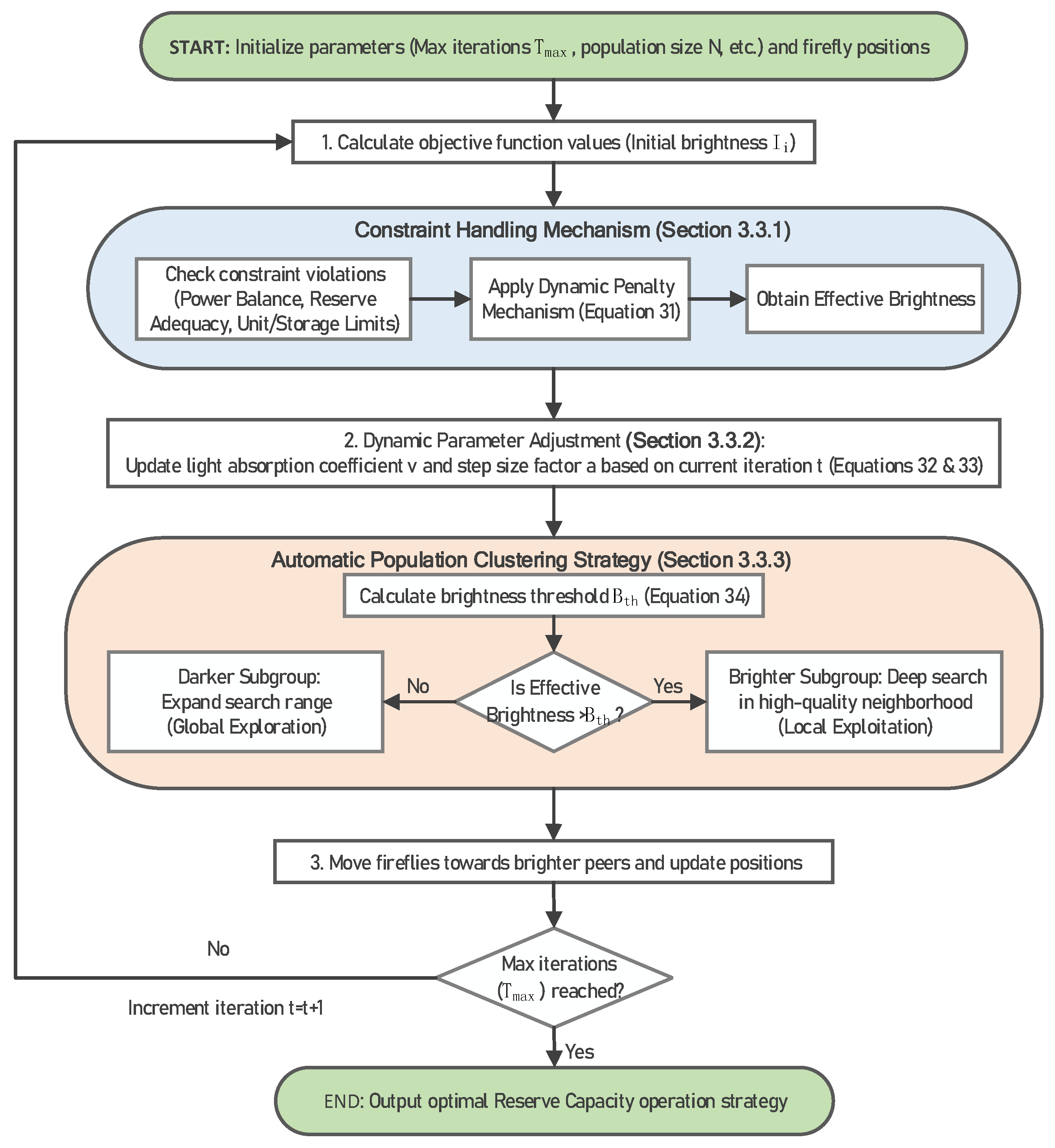
To ensure solution feasibility, a Dynamic Penalty Mechanism is incorporated into the brightness calculation. This mechanism penalizes solutions violating Power Balance, reserve adequacy, Unit Operating Constraints, or energy storage system limitations. The resulting effective brightness after penalty adjustment is defined as follows:

$$I=I_0 \cdot e^{-\gamma r_{ij}} -\lambda \cdot {\displaystyle \sum _{m}max(0,g_m (x))}$$

(31)

$I_0 \cdot e^{-\gamma r_{ij}}$ denotes the definition of the firefly’s relative fluorescence intensity in the standard algorithm; $I_0$ represents the firefly’s maximum fluorescence intensity, which correlates with the objective function value; $\gamma$ signifies the light intensity absorption coefficient; $r_{ij}$ indicates the spatial distance between the firefly and the target; $g_m (x)$ measures the violation degree of the $m$ constraint; and $\lambda$ represents the dynamic penalty factor. This mechanism prevents infeasible solutions from competing for the optimal solution, thereby enhancing search efficiency.

3.3.2. Dynamic Parameter Adjustment

The incorporation of problem characteristics, dynamically adjusted light intensity absorption coefficients, and step size factors is instrumental in the effective balancing of solution quality and convergence speed.

$$\gamma (t)={\gamma }_{max} -({\gamma }_{max} -{\gamma }_{min} )\cdot {\displaystyle \frac{t}{Maxlter}}$$

(32)

$$\alpha (t)={\alpha }_{max} \cdot e^{-ln({\alpha }_{max} /{\alpha }_{min})\cdot t/Maxlter}$$

(33)

$\gamma (t)$ and $\alpha (t)$ refer to light intensity absorption coefficient and step size factor at iteration $t$; ${\gamma }_{max}$ and ${\gamma }_{min}$ denote the maximum and minimum light intensity absorption coefficients; ${\alpha }_{max}$ and ${\alpha }_{min}$ correspond to the maximum and minimum step size factors; $Maxlter$ indicates the maximum iteration count. During the early iteration phase, $\gamma$ is small and $\alpha$ is large, enhancing global exploration capabilities; in the later phase, $\gamma$ increases while $\alpha$ decreases, shifting toward localized fine-grained search.

3.3.3. Automatic Population Clustering Strategy

The execution of real-time swarm division is contingent upon the brightness of fireflies, with the purpose of guiding brighter subgroups to conduct deep searches within high-quality solution neighborhoods.

$$B_{th}={\displaystyle \frac{1}{N}}{\displaystyle \sum _{i=1}^N{I}_i^{\prime } (t)} +\mathcal{\sigma }(t)$$

(34)

$B_{th}$ represents the brightness threshold for the $t$ generation; $N$ denotes the population size; $I_i^{\prime } (t)$ signifies the effective brightness of the $i$ firefly; and $\mathcal{\sigma }(t)$ indicates the standard deviation of brightness. Subgroups with brightness exceeding $\mathcal{\sigma }(t)$ undergo deep search within the high-quality solution neighborhood, while subgroups below $\mathcal{\sigma }(t)$ expand their search range to prevent premature convergence.

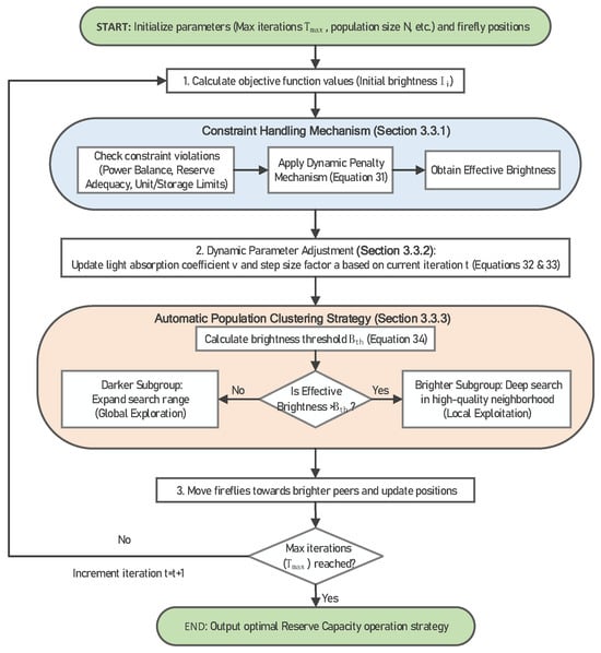
The aforementioned improvements enable the algorithm to outperform traditional optimization methods in terms of solution quality and convergence speed, rendering it particularly suitable for multi-period, multi-device coordinated reserve capacity optimization problems. The specific workflow of the optimization algorithm is illustrated in Figure 3.

Figure 3. Optimization Algorithm Flowchart.

4. Case Study Analysis

To validate the effectiveness and superiority of the proposed method, this chapter employs a typical urban integrated energy system (UIES) case study to sequentially perform reserve demand quantification and operational optimisation. All model construction, scenario generation, and optimization solutions in this research were completed within the same integrated environment. Algorithm development and numerical experiments were carried out using MATLAB R2024b on Windows 11. Firstly, a test case incorporating wind power, photovoltaic, thermal power units, and energy storage is constructed with parameters set. Subsequently, the reserve requirement for each period during a typical day is expressed quantitatively. In conclusion, a refined firefly optimisation algorithm is utilised to address the constructed model, thereby attaining the optimal distribution of reserve capacity.

4.1. Basic Parameter Settings

This case study is constructed based on the energy structure of a typical city in China, with the aim of enhancing the integration capacity of fluctuating renewable energy sources while ensuring the reliability of power supply. The primary system parameters are delineated in Table 1. The unit generation cost for thermal power units references relevant studies on the levelised cost of electricity for coal-fired power plants, reflecting their primary variable fuel costs [23]. The unit standby cost for all equipment primarily represents the opportunity cost of lost generation due to reserved capacity. As energy storage enables rapid response with no start-stop losses, its standby cost should be lower than that of thermal power units. Specifically, the ageing costs of electrochemical energy storage are directly correlated with its depth of charge/discharge and charge/discharge rate [24]. This paper sets the operational costs for charging and discharging of the energy storage system at 0.15 CNY/kWh and 0.25 CNY/kWh, respectively, to more accurately reflect the additional ageing costs and energy losses incurred during the discharge process. Furthermore, the table incorporates start-stop costs for thermal units, stipulating a minimum start-stop duration of 4 h per unit. These costs are calculated using industry-standard estimation methods (equivalent to the cost of operating at full load for several hours). It is important to note that this research focuses on the optimal dispatch of system operations. Within this framework, capital investment, fixed operation and maintenance costs, and other non-related costs of the generation units are not considered as decision variables in the optimization. Consequently, the model only accounts for operational costs (i.e., variable costs) that are directly influenced by dispatch decisions, including fuel costs, start-up and shut-down costs, and output-dependent maintenance costs.

Table 1. Key System Parameters.

Parameter Type	Parameter Name	Parameter Value	Unit
Load	Peak Load	1000	kW
Photovoltaic System	Rated Capacity	800	kW
Wind Power System	Rated Capacity	100	kW
Thermal Power Unit	Unit Capacity	200	kW
	Number of Units	5	kW
	Total installed capacity	1000	kW
	Minimum Technical Output Coefficient	0.3	-
	Unit Generation Cost	0.35	CNY/kWh
	Unit reserve cost	0.2	CNY/kW
	Minimum start-stop hours	4	Hour
	Start-stop costs	280	CNY
Energy Storage System	Maximum charging power	250	kW
	Maximum Discharging Power	250	kW
	Rated Energy Storage Capacity	370	kWh
	SOC Operating Upper Limit	0.9	-
	SOC Operating Lower Limit	0.1	-
	Initial SOC	0.5	-
	Average Charge/Discharge Cost	0.15/0.25	CNY/kWh
	Unit reserve cost	0.15	CNY/kW

Meanwhile, we design two contrasting typical scenarios for analysis, as outlined below:

Scene I: Corresponding to a typical summer day, it is characterized by high solar irradiance and low wind speed, simulating an operational environment where photovoltaic output is abundant while the contribution from wind power is relatively low.

Scene II: Corresponding to a typical winter day, it features low solar irradiance and high wind speed, representing an operational state where photovoltaic output diminishes and wind power becomes the dominant variable energy source.

This comparative design aims to thoroughly reveal the differences in renewable energy output structures under distinct seasonal climate patterns and their specific impacts on system reserve requirements and dispatch strategies.

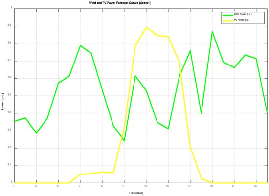
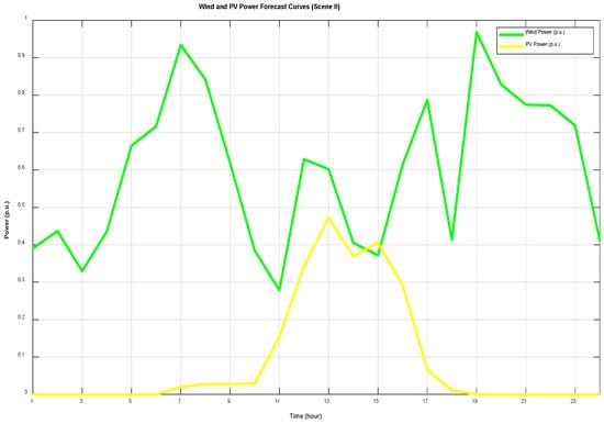
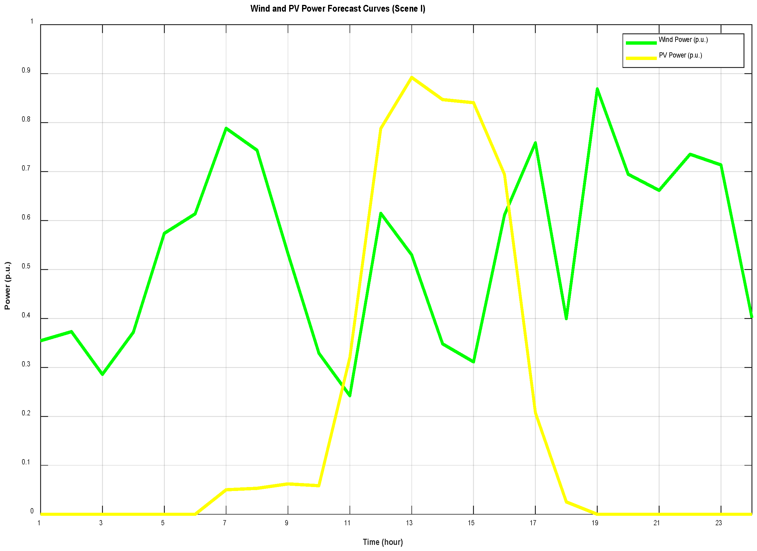
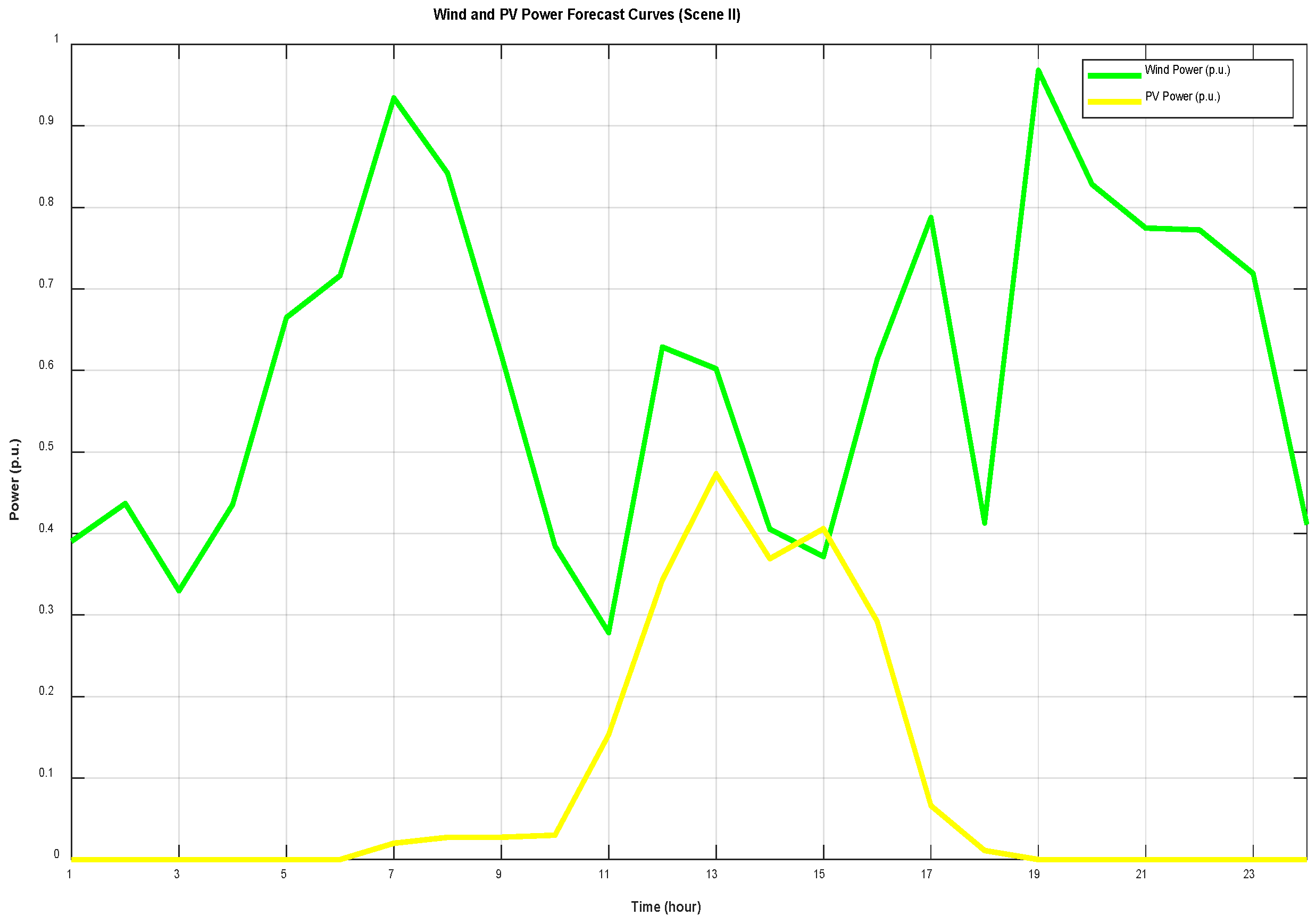
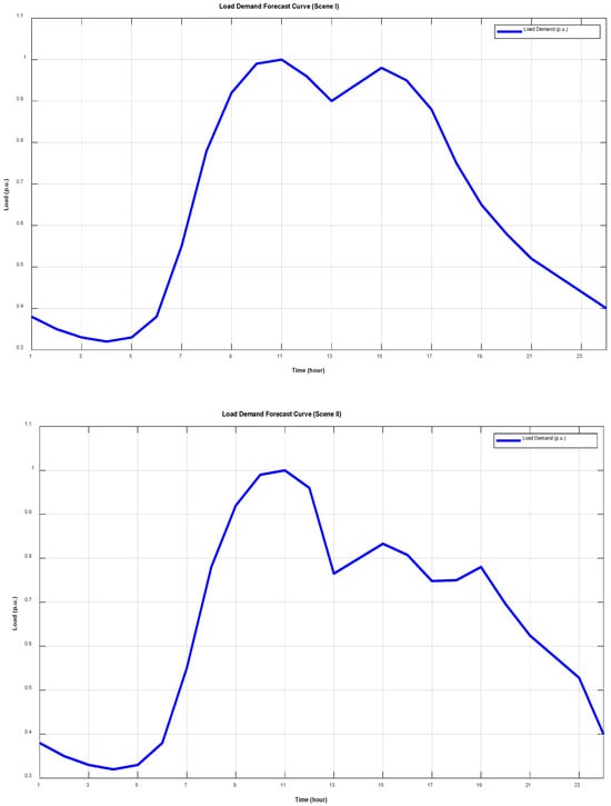
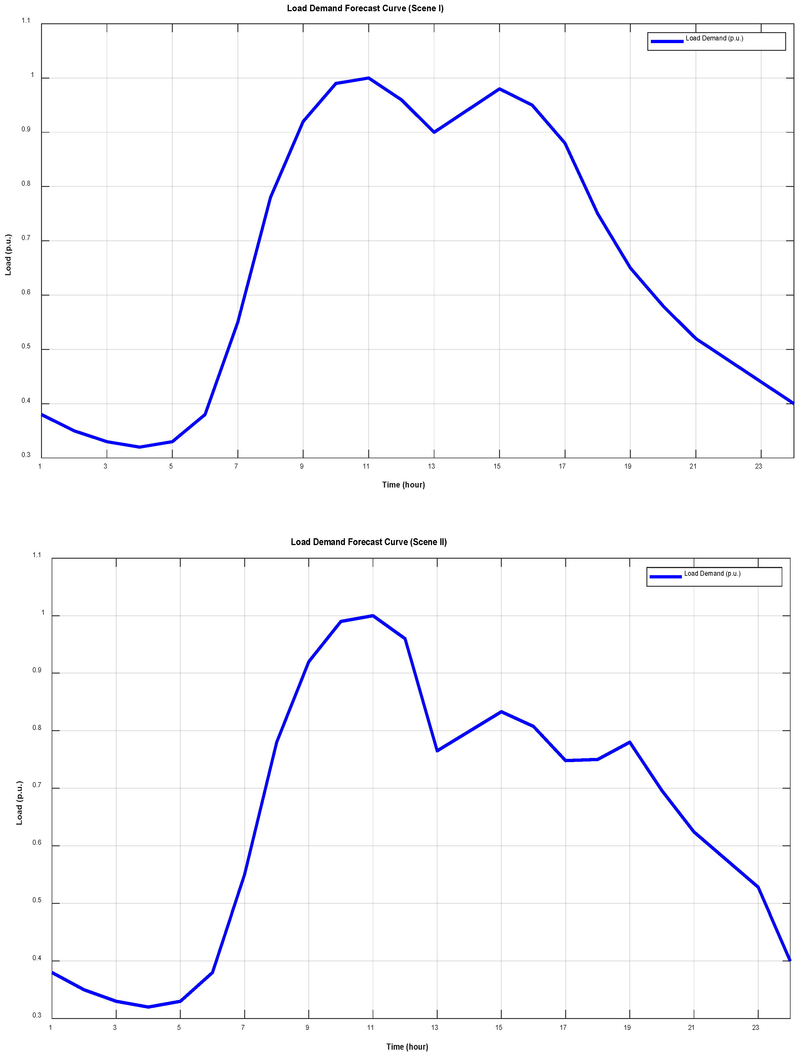
The external environmental parameters considered for system operation primarily include forecast values and uncertainty parameters for wind power, photovoltaic power, and load. Photovoltaic output exhibits distinct diurnal characteristics, with higher daytime and lower nighttime levels, while the standardized value of wind power output ranges from 0.3 to 0.8. The characteristic curves of the aforementioned subjects are displayed in Figure 4. In addition, Figure 4 shows that, compared with Scene I, Scene II features lower photovoltaic output and a higher contribution from wind power, indicating a shift in the dominant renewable energy source under winter conditions. Conversely, load demand exhibits a typical double-peak pattern, as demonstrated in Figure 5. Figure 5 also shows that under Scene II, the load demand curve differs in both magnitude and temporal distribution compared with Scene I, indicating distinct seasonal load characteristics associated with winter operating conditions.

Figure 4. Predicted Curves of Wind Power and PV Output Standardized Values.

Figure 5. Load Demand Standardized Value Forecast Curve.

In order to quantify the reserve requirement of the system, it is necessary to clearly define specific parameters for various uncertainties. As illustrated in Table 2, the primary settings encompass wind and solar forecasting errors, along with equipment failure rates. These parameters will serve as the foundation for subsequent reserve requirement analysis.

Table 2. Uncertainty and Reserve Parameters.

Parameter Category	Parameter Name	Parameter Value
Prediction Error	Wind Power Error Standard Deviation Coefficient	10%
	Photovoltaic Error Standard Deviation Coefficient	10%
	Load error coefficient	5%
Equipment failure	Minimum Failure Rate (30% Load)	2%
	Maximum Failure Rate (100% Load)	5%
Confidence Level	Reserve Requirement confidence level	99%
Scenario Settings	Initial Scenario Count	1000
	Number of Typical Scenarios	10

Furthermore, in order to effectively solve the high-dimensional, non-convex Reserve-Capacity-Oriented Operational Optimization Model, this section proposes to adopt the improved firefly algorithm (IFA) introduced earlier. Through dynamic parameter adjustment, constraint handling mechanisms, and population partitioning strategies, this algorithm significantly enhances computational performance for complex optimisation problems. The specific parameter settings are delineated in Table 3.

Table 3. Parameter Settings for the improved firefly algorithm (IFA).

Parameter Name	Parameter Value
Population Size	100
Maximum Iterations	500
Maximum Attractance β0	1.0
Light Absorption Coefficient γ Range	[0.01, 1.0]
Step factor α range	[0.001, 0.1]
Initial Penalty Factor	100
Clustering ratio threshold	0.6
Brightness standard deviation weight	0.5

4.2. Quantification of Reserve Requirement

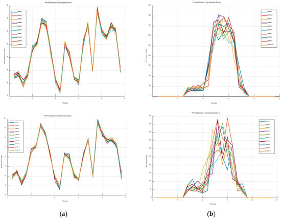
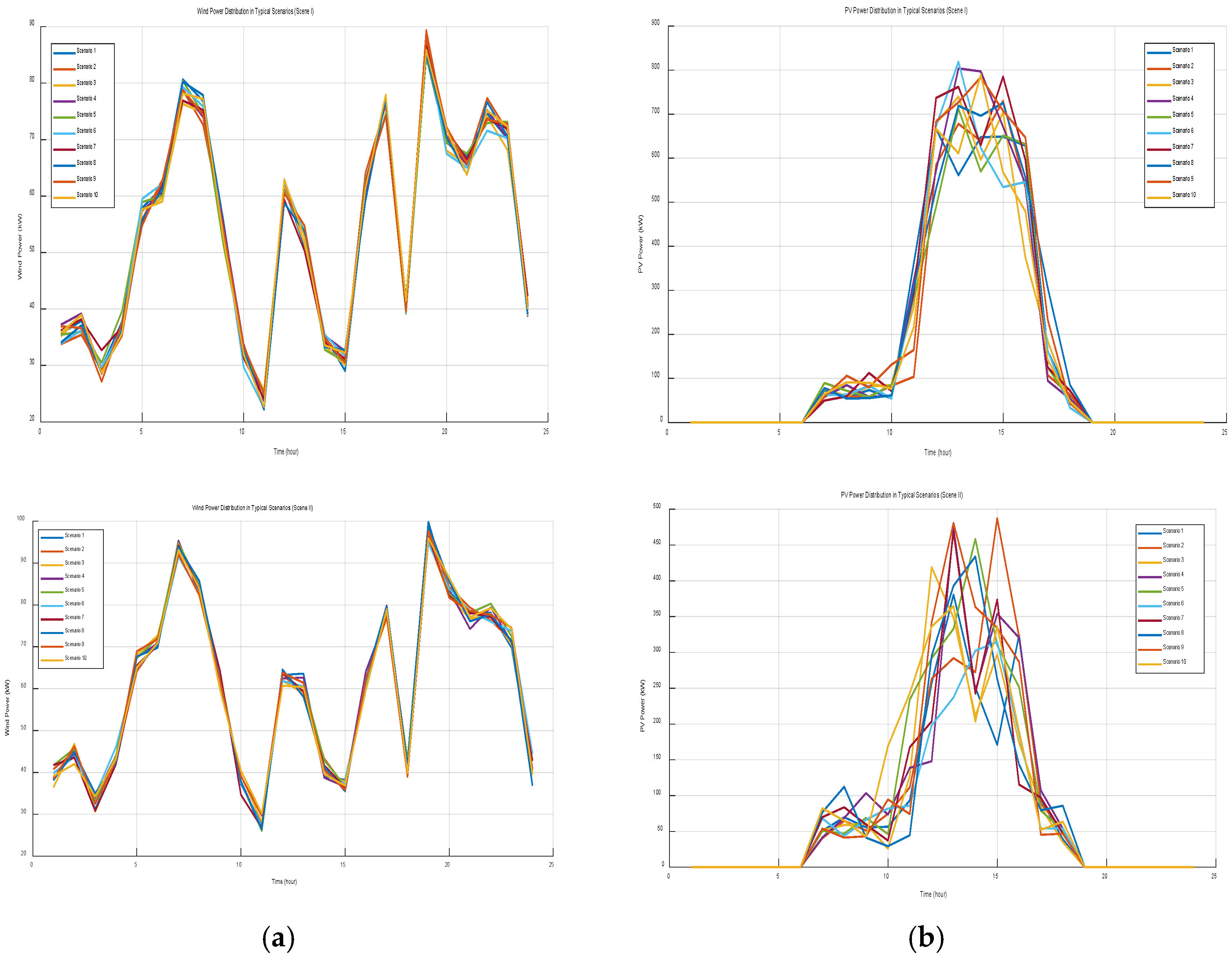
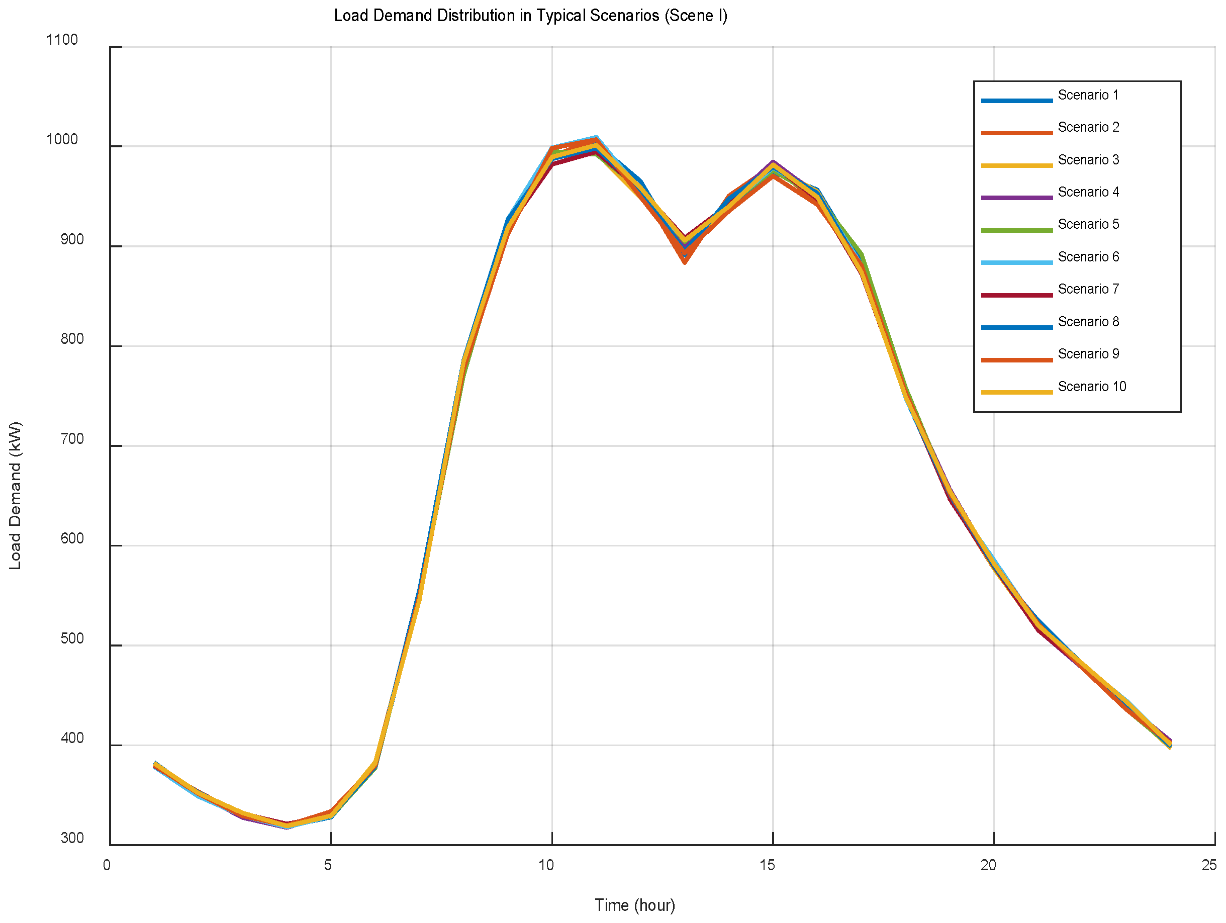
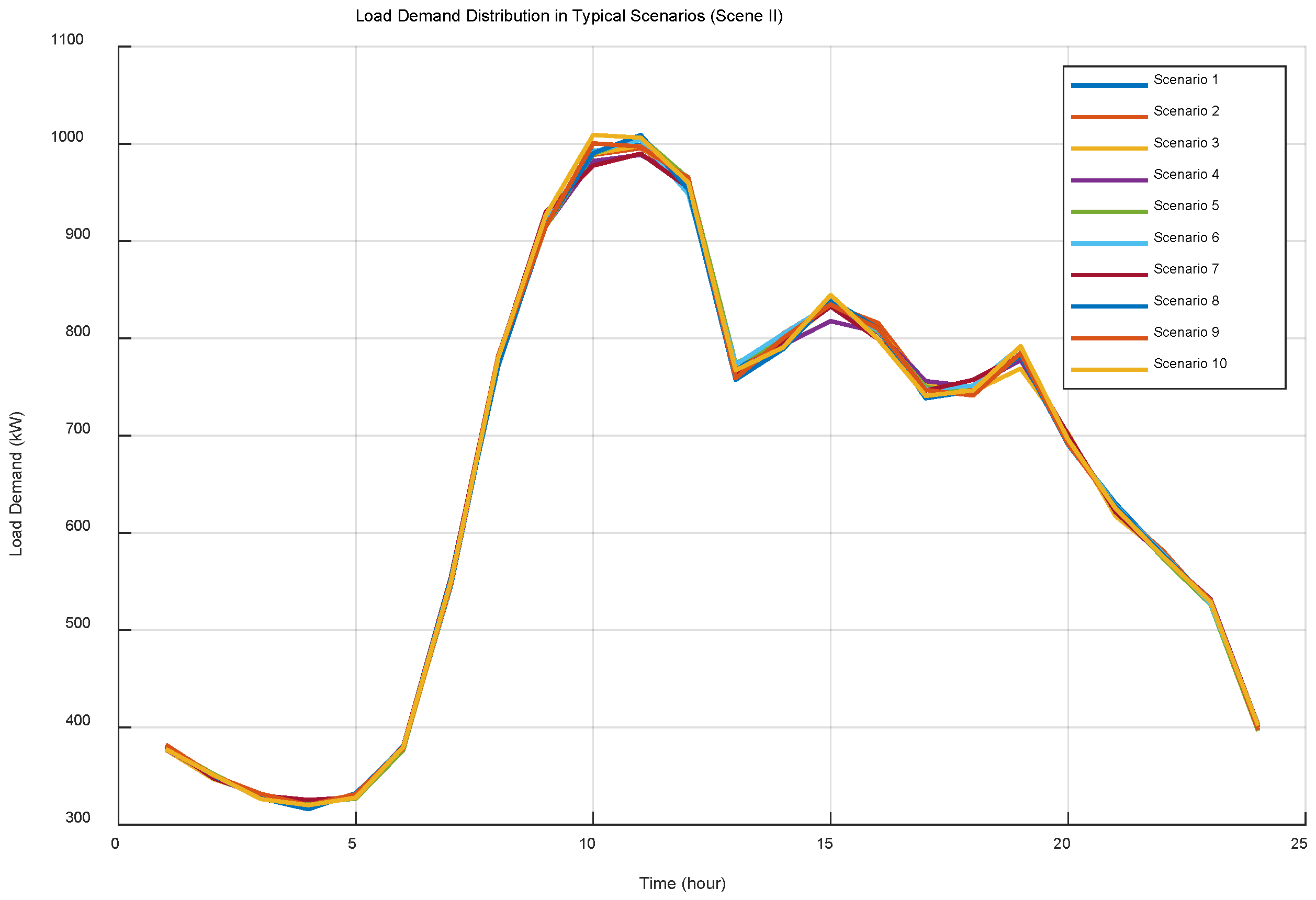
In accordance with the multi-source uncertainty reserve demand quantification model established in Section 2, this section employs Monte Carlo Simulation in sequence for the generation of scenarios, calculates equipment failure probability, and ultimately quantifies the system reserve requirement. Specifically, following the methodology outlined in Section 2.1, a Monte Carlo Simulation is first employed to generate an initial set of scenarios incorporating joint uncertainties in wind, solar, and load. Subsequently, K-means clustering is employed for the purpose of scenario reduction, yielding representative typical scenarios. Figure 6 and Figure 7, respectively, illustrate the probability distributions of wind power output, solar power output, and load demand under typical scenarios. These distributions effectively capture the complementary characteristics of wind power and solar power generation alongside the temporal fluctuations of load demand, providing a reliable foundation for subsequent reserve requirement analysis.

Figure 6. (a) Description of wind power distribution in typical scenarios; (b) Description of solar power distribution in typical scenarios.

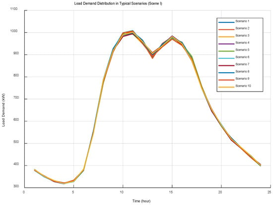
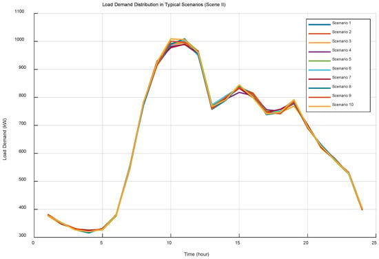
Figure 7. Load Demand Distribution in Typical Scenarios.

Figure 6a,b present the probability distributions of wind power and photovoltaic output under typical scenarios. The distributions capture the complementary characteristics of wind and solar generation. Figure 6a further shows that the wind power distribution under Scene II differs from that of Scene I, reflecting seasonal changes in wind resource characteristics. Similarly, Figure 6b indicates a distinct photovoltaic output distribution under Scene II compared with Scene I, consistent with the scenario labels shown in the figure.

Figure 7 illustrates the load demand distribution under typical scenarios. The figure further indicates that the load demand distribution under Scene II differs from that under Scene I, reflecting seasonal differences in load demand characteristics as labelled in the subfigures.

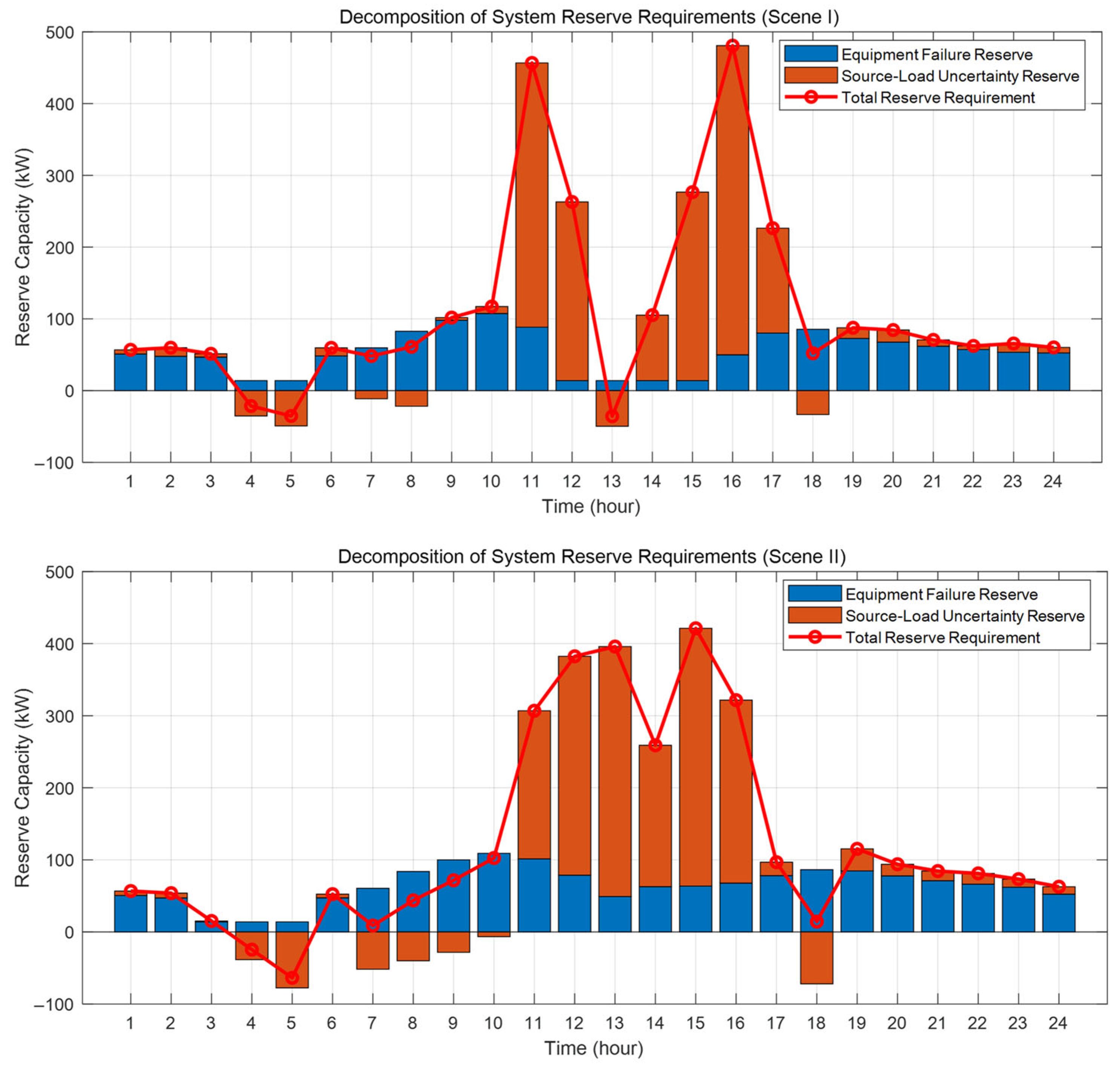
Concurrently, the equipment failure reserve for each period was calculated on the basis of the load factor-related failure probability model established in Section 2.2 and the failure parameters referenced in Table 2. Based on this, the reserve requirement triggered by source-load uncertainty is superimposed. Finally, using the probabilistic definition outlined in Section 2.3, an integrated overview of the system’s reserve requirement for each period is obtained, with the results shown in Figure 8.

Figure 8. System Reserve Requirement Component Breakdown Diagram.

Quantitative results indicate that, taking Scene I as an example, analysis shows the system’s daily reserve requirement fluctuates between −100 kW and 500 kW. Specifically, equipment failure reserves have been shown to correlate with thermal unit load factors, remaining relatively stable and consistently below 100 kW. In contrast, source-load uncertainty reserves have been observed to exhibit significant fluctuations, constituting the primary driver of total demand variation. It is noteworthy that the system encountered an upward reserve peak of approximately 350 kW between 11:00 and 12:00, succeeded by a downward reserve peak of approximately −100 kW during the 13th hour. This was primarily caused by sharp fluctuations in Net Load, resulting from a sudden surge in photovoltaic output during midday. Figure 8 also indicates that under Scene II, reserve requirements exhibit a different temporal pattern, which is associated with the higher contribution of wind power shown in Figure 4, leading to reserve demand being driven primarily by wind-related uncertainty rather than photovoltaic fluctuations.

4.3. Analysis of Reserve Capacity Operation Optimization Results Based on IFA

In accordance with the principles set out in Section 3 concerning the Reserve-Capacity-Oriented Operational Optimization Model, and in consideration of the quantification of reserve requirements as delineated in prior analyses, the implementation of the improved firefly algorithm (IFA) is a viable methodology for determining the optimal output for each system component and the reserve capacity allocation plan.

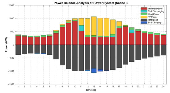
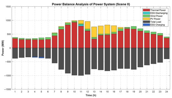
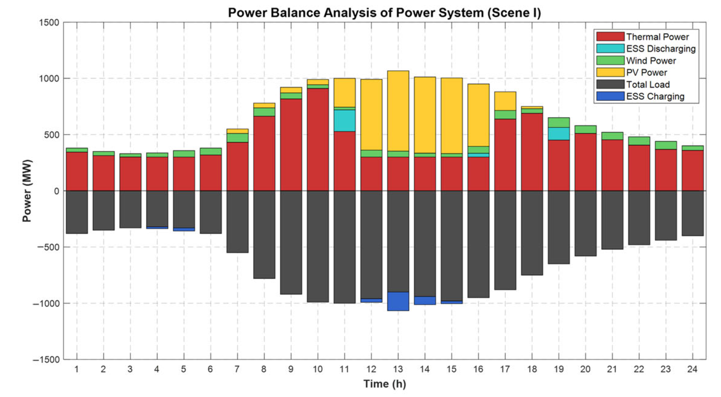
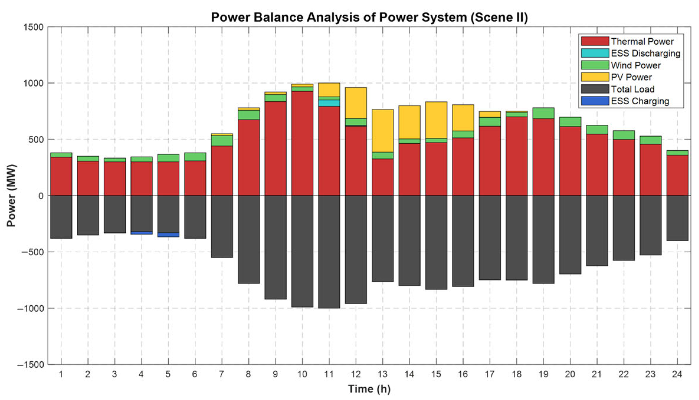
It is evident that, at the system power balance level, the system’s power balance is achieved through the coordinated operation of thermal power generation and energy storage. In instances where the net load is negative, the energy storage system is utilised for the purpose of absorbing excess renewable energy. In periods of positive net load, the primary responsibility for power supply falls to thermal power units, with energy storage units discharging as required to assist in peak shaving.

Figure 9 further shows that under Scene II, the overall power balance mechanism remains unchanged, while the relative contributions of wind power and thermal units differ due to the altered renewable generation mix.

Figure 9. System Power Balance Optimization Results.

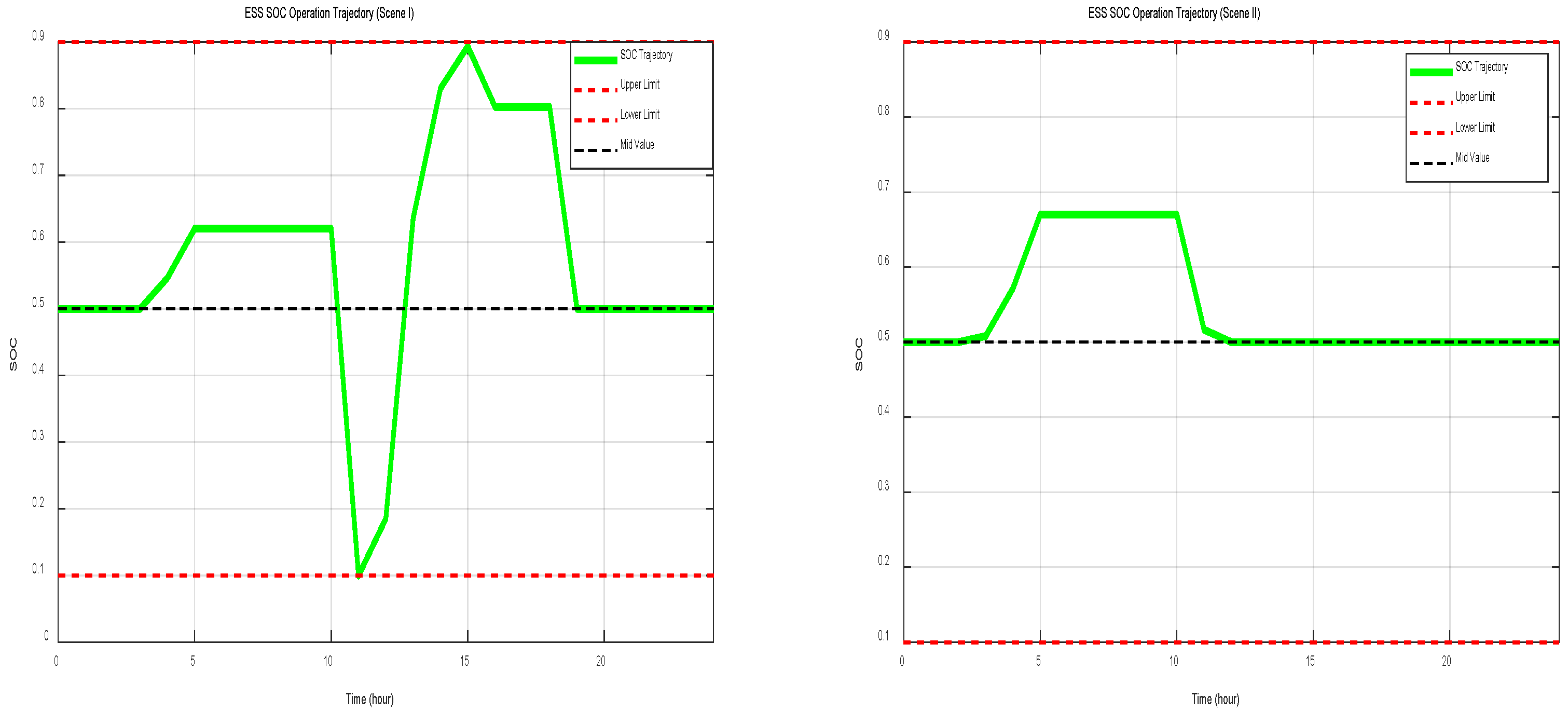
As demonstrated in Figure 10, the energy storage system’s state of charge (SOC) remained within the acceptable range throughout the entire scheduling cycle. Ultimately, the energy storage system’s SOC returned to its initial value, thereby facilitating operational optimisation for the subsequent operating day. Figure 10 also shows that the SOC trajectory under Scene II follows a different temporal pattern, reflecting the change in renewable generation characteristics between the two scenarios.

Figure 10. Energy Storage System SOC Operational Trajectory.

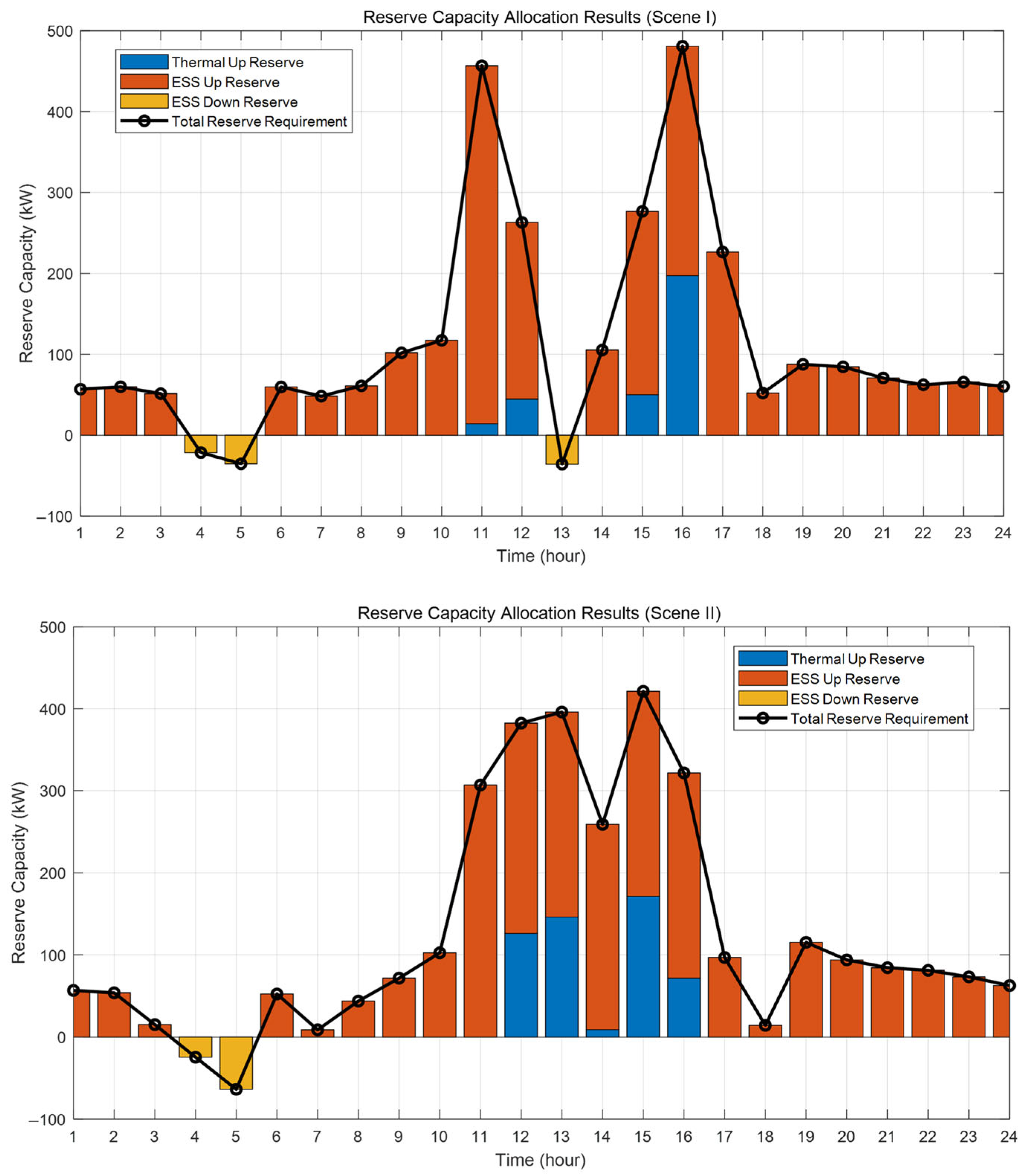
As demonstrated in Figure 11, the optimized allocation scheme takes into full account the regulatory characteristics of the various resources. In contrast to Power Balance, energy storage systems are responsible for the primary upward reserve task, with thermal units providing only a minor amount of upward reserve capacity at 12:00 and 15:00. Conversely, energy storage provides all downward reserve, leveraging its rapid response advantage. Figure 11 further indicates that under Scene II, thermal power units contribute a relatively larger share of upward reserve compared with Scene I, while energy storage remains the main provider of downward reserve.

Figure 11. Optimized Reserve Capacity Allocation Results.

Under Scene I, the total daily operating cost of the system is 2264.02 CNY, as shown in Table 4. From a cost structure perspective, system operating costs primarily consist of energy supply costs and reserve service costs. Specifically, energy supply costs, including thermal generation cost and ESS operating cost, account for 81.18% of the total operating cost, while reserve service costs account for the remaining 18.82%. Among these components, thermal generation cost represents the largest share at 75.21%. In addition, the ESS reserve cost accounts for 17.69% of the total cost, which is significantly higher than its operating cost share of 5.97%. This cost distribution indicates that, under Scene I, the proposed operational optimisation model effectively balances the economics of energy supply and reserve allocation while ensuring system reliability. The relatively high proportion of reserve-related costs further highlights the pivotal role of the energy storage system in providing high-value reserve services and enhancing operational flexibility.

Table 4. Comparison of Economic Indicators.

	Scene I	Scene II
Thermal Generation Cost (CNY)	1702.75	2654.51
ESS Operating Cost (CNY)	135.27	25.24
Thermal Power Reserve Costs (CNY)	25.43	52.37
ESS Reserve Cost (CNY)	400.57	390.78
Total (CNY)	2264.02	3122.89

Under Scene II, the total operating cost increases to 3122.89 CNY. As indicated by the cost components in Table 4, thermal generation cost and reserve-related costs both increase in absolute terms, reflecting higher reliance on thermal units and increased reserve requirements under winter operating conditions. Although the ESS operating cost decreases, the ESS reserve cost remains a significant component of the total cost, demonstrating that energy storage continues to play a crucial role in reserve provision.

5. Conclusions

This paper has investigated reserve-capacity-oriented operation of an urban integrated energy system (UIES) under multiple uncertainties, and proposed a unified framework covering uncertainty modelling, reserve requirement quantification, operational optimisation and algorithm design.

First, a multi-source uncertainty model was established that integrates wind and photovoltaic output variability, load forecasting errors and equipment failure risks into a single scenario-based framework. By combining Monte Carlo scenario generation, scenario reduction and a load-factor-based piecewise failure probability model, the approach enables a refined representation of upward and downward reserve requirements over the scheduling horizon.

Second, a reserve-capacity-oriented operational optimisation model was formulated to minimise total system operating cost, including generation cost and reserve cost, subject to power balance, reserve adequacy, unit operating constraints and energy storage charging/discharging and SOC constraints. This model explicitly coordinates conventional thermal units and the energy storage system as the main reserve providers, and embeds engineering constraints such as the coupling between unit output and reserve capacity.

Third, a case study of a typical urban system with wind power, photovoltaic units, thermal units and an energy storage system was carried out to validate the proposed method. The quantified reserve requirement fluctuates between −100 kW and 500 kW over a typical day. Equipment-failure-related reserve remains relatively stable and below 100 kW, whereas the reserve induced by source–load uncertainty exhibits pronounced variations and dominates the total demand. In the summer scenario, characterized by high solar irradiance, the system experiences a concentrated upward reserve peak of about 350 kW around midday, driven by sharp photovoltaic output fluctuations. In contrast, the winter scenario, with higher wind penetration, presents a different reserve profile where upward demand, though slightly lower in peak magnitude, is sustained at a higher baseline throughout the day to manage wind power volatility. On the operational side, thermal generation and the energy storage system jointly maintain power balance in both cases, with storage absorbing excess renewable energy when net load is negative and discharging to assist peak shaving when net load is positive. Energy storage is also identified as the primary provider of both upward and downward reserve, leveraging its fast response capability. The total operating costs for the summer and winter scenarios are 2264.02 CNY and 3122.89 CNY, respectively. The cost structure analysis reveals that while thermal generation constitutes the largest cost share (75.21% in summer, increasing to 85.01% in winter), ESS reserve cost remains a significant component (17.69% in summer, 12.51% in winter). This cost structure indicates that reserve services constitute a non-negligible share of total expenditure, and that the economic value of the energy storage system in this scheme is mainly realised through reserve provision rather than pure energy arbitrage.

Overall, the proposed reserve-capacity-oriented operation optimisation method shows good feasibility and effectiveness from both modelling and application perspectives, and provides a practical reference for secure and economical operation of UIES with high renewable penetration. Future work may further extend this framework towards multi-timescale coordination between different reserves, deeper integration with market mechanisms and price-based incentives, and broader consideration of multi-energy coupling in real urban applications.

References

- Doherty, R.; O’Malley, M. A new approach to quantify reserve demand in systems with significant installed wind capacity. IEEE Trans. Power Syst. 2005, 20, 587–595. [Google Scholar] [CrossRef] [Scilit]
- Dong, J.; Fu, A.; Liu, Y.; Nie, S.; Yang, P.; Nie, L. Two-stage optimization model for two-side daily reserve capacity of a power system considering demand response and wind power consumption. Sustainability 2019, 11, 7171. [Google Scholar] [CrossRef] [Scilit]
- Hassan, M.W.; Rasheed, M.B.; Javaid, N.; Nazar, W.; Akmal, M. Co-Optimization of Energy and Reserve Capacity Considering Renewable Energy Unit with Uncertainty. Energies 2018, 11, 2833. [Google Scholar] [CrossRef] [Scilit]
- Lu, S.; Wu, Y.; Lou, S.; Yin, X. A Model for Optimizing Spinning Reserve Requirement of Power System Under Low-carbon Economy. IEEE Trans. Sustain. Energy 2014, 5, 1048–1055. [Google Scholar] [CrossRef] [Scilit]
- Ortega-Vazquez, M.A.; Kirschen, D.S. Optimizing the spinning reserve requirements using a cost/benefit analysis. IEEE Trans. Power Syst. 2007, 22, 24–33. [Google Scholar] [CrossRef] [Scilit]
- Eltohamy, M.; Talaat, H.; Moteleb, M.; Mekhamer, S.; Omran, W.A. Probabilistic Methodology for Estimating Reserve Requirement and Optimizing Its Components in Systems with High Wind Penetration. IEEE Access 2022, 10, 106148–106168. [Google Scholar] [CrossRef] [Scilit]
- Pan, C.; Shao, C.; Hu, B.; Xie, K.; Li, C.; Ding, J. Modeling the Reserve Capacity of Wind Power and the Inherent Decision-Dependent Uncertainty in the Power System Economic Dispatch. IEEE Trans. Power Syst. 2023, 38, 4404–4417. [Google Scholar] [CrossRef] [Scilit]
- Yang, Y.; Meng, Z.; Wu, G.; Yang, Z.; Guo, R. A Probabilistic Reserve Decision-Making Method Based on Cumulative Probability Approximation for High-Penetration Renewable Energy Power System. Energies 2025, 18, 2658. [Google Scholar] [CrossRef] [Scilit]
- Zhang, F.; Qiao, Y.; Lu, Z.X. Extreme wind power forecast error analysis considering its application in day-ahead reserve capacity planning. Renew. Power Gener. 2018, 12, 1923–1930. [Google Scholar] [CrossRef] [Scilit]
- Li, B.; Li, H.; Liang, Z.; Bai, X. Load Day-Ahead Automatic Generation Control Reserve Capacity Demand Prediction Based on the Attention-BiLSTM Network Model Optimized by Improved Whale Algorithm. Energies 2024, 17, 415. [Google Scholar] [CrossRef] [Scilit]
- Zheng, Z.; Chen, G.; Shen, Z.; Dong, Z. Data-driven robust optimization for energy and reserve scheduling considering multi-uncertainty. Int. J. Electr. Power Energy Syst. 2025, 169, 110751. [Google Scholar] [CrossRef] [Scilit]
- Kim, I. Optimal capacity of storage systems and photovoltaic systems able to control reactive power using the sensitivity analysis method. Energy 2018, 150, 642–652. [Google Scholar] [CrossRef] [Scilit]
- Yuan, B.; Zhou, J.; Lu, G.; Liu, D.; Xia, P.; Wu, C. Coordinated Dispatch of Power Generation and Spinning Reserve in Power Systems with High Renewable Penetration. Processes 2024, 12, 2779. [Google Scholar] [CrossRef] [Scilit]
- Yang, X.; Zhao, Y.; Li, Y.; Huang, C.; Ding, Q. Generation Maintenance Scheduling for Power Systems Considering the Risk Quantification of Hybrid Uncertainty. IEEE Trans. Power Syst. 2025, 40, 3499–3512. [Google Scholar] [CrossRef] [Scilit]
- Khazali, A.; Kalantar, M. Spinning Reserve Quantification by a Stochastic–Probabilistic Scheme for Smart Power Systems with High Wind Penetration. Energy Convers. Manag. 2015, 96, 242–257. [Google Scholar] [CrossRef] [Scilit]
- Liu, L.; Hu, Z.; Wen, Y.; Ma, Y. Modeling of Frequency Security Constraints and Quantification of Frequency Control Reserve Capacities for Unit Commitment. IEEE Trans. Power Syst. 2024, 39, 2080–2092. [Google Scholar] [CrossRef] [Scilit]
- Jun, D.; Nie, L.; Nie, S.; Yang, P.; Fu, A. Two-Stage Robust Optimization Model for Spinning Reserve Capacity Considering Demand Response and Uncertainty of Wind Power. Electr. Power Constr. 2025, 40, 55–64. [Google Scholar]
- Zhang, N.; Li, Y.; Ding, Q.; Zhang, X.; Jiang, H.; Li, W. An Inertia Reserve Capacity Planning Method for Power Systems Considering Risk Preference. IEEE Access 2024, 12, 87728–87741. [Google Scholar] [CrossRef] [Scilit]
- Lei, K.; Chang, J.; Wang, X.; Guo, A.; Wang, Y.; Ren, C. Peak shaving and short-term economic operation of hydro-wind-PV hybrid system considering the uncertainty of wind and PV power. Renew. Energy 2023, 215, 118903. [Google Scholar] [CrossRef] [Scilit]
- Zhang, Y.; Le, J.; Zheng, F.; Zhang, Y.; Liu, K. Two-stage distributionally robust coordinated scheduling for gas-electricity integrated energy system considering wind power uncertainty and reserve capacity configuration. Renew. Energy 2019, 135, 122–135. [Google Scholar] [CrossRef] [Scilit]
- Duan, J.; Liu, F.; Yang, Y.; Jin, Z. Two-stage flexible economic dispatch for power system considering wind power uncertainty and demand response. Energy Sources 2022, 44, 650–668. [Google Scholar] [CrossRef] [Scilit]
- Zhu, J.; Xiong, X.; Liu, Q.; Xuan, P.; Xie, P.; Zou, J. Economic dispatch considering joint wind-photovoltaic forecast errors in electricity spot markets. Acta Energiae Solaris Sin. 2021, 42, 450–458. [Google Scholar]
- Xi, J.; Zhang, B.; Yang, Y. Calculation and Monte Carlo uncertainty analysis of the levelized cost of electricity for different energy power generation in the smart grid under time scales. Energy Strategy Rev. 2025, 58, 101666. [Google Scholar] [CrossRef] [Scilit]
- Luan, T.; Yang, Z.; Li, J.; Zheng, Y.; Feng, S. Electricity market mechanism design considering cost characteristics of electrochemical energy storage. Autom. Electr. Power Syst. 2024, 48, 101–110. [Google Scholar]
Disclaimer/Publisher’s Note: The statements, opinions and data contained in all publications are solely those of the individual author(s) and contributor(s) and not of MDPI and/or the editor(s). MDPI and/or the editor(s) disclaim responsibility for any injury to people or property resulting from any ideas, methods, instructions or products referred to in the content. |
© 2026 by the authors. Licensee MDPI, Basel, Switzerland. This article is an open access article distributed under the terms and conditions of the Creative Commons Attribution (CC BY) license.