


Abstract
Accurate state identification is crucial for the safe and efficient operation of renewable energy systems. However, monitoring data from photovoltaic (PV) and wind power systems often suffer from significant class imbalance. This imbalance reduces state recognition accuracy. In this study, we propose one framework to augment fault data and recognize operating states for a combined PV–wind system. The framework first converts signals into images using the Gramian Angular Summation Field (GASF). It then groups samples with K-means clustering. Next, a deep convolutional generative adversarial network (DCGAN) generates additional fault samples for minority classes. Finally, a two-dimensional convolutional neural network (2D-CNN) identifies the operating state. PV and wind time-series signals are first mapped into 2D images via GASF to yield richer spatial-feature representations, and K-means clustering is then used to define operating states in an unsupervised manner and generate the corresponding labels. In PV-only, wind-only, and combined PV–wind scenarios, the baseline 2D-CNN trained on imbalanced datasets achieves recognition accuracies of 95.89%, 57.93%, and 81.94%, respectively. To alleviate class imbalance, DCGAN is employed to synthesize images and construct balanced datasets; the best recognition accuracies in the three scenarios increase to 99.20%, 97.08%, and 97.62%, and the model shows stronger robustness in identifying minority classes. This approach supports both single-source applications and multi-source systems such as large-scale wind–solar bases by providing data and algorithmic foundations for generalized fault-diagnosis models, thereby enabling more reliable, data-driven operational monitoring.
Keywords:
photovoltaic; wind power; GASF; K-means clustering; DCGAN; 2D-CNN; imbalanced data; state recognition accuracy 1. Introduction
Research Background and Significance
The world is moving toward a low-carbon energy system. Renewable energy is now a main source of growth in electricity supply. The International Energy Agency (IEA) expects renewables to meet more than 90% of global electricity demand growth from 2025 to 2030 [1]. The IEA’s outlook for the period before 2025 further indicates that, by 2025, newly added renewable power capacity will be dominated by solar photovoltaics at about 60%, while wind power will contribute roughly 30% [2]. PV and wind installations keep growing. Their stable operation affects both system reliability and project revenue. PV array fault diagnosis needs to be fast and accurate. If faults persist, they can damage modules and may even trigger fire risks [3]. In the wind sector, condition-based maintenance emphasizes real-time state monitoring; once performance degradation or fault signatures appear, timely maintenance can reduce unexpected failures, improve availability, and lower maintenance costs [4]. In real projects, operation and maintenance data from PV and wind systems often show strong class imbalance. Wind turbines run in normal states for most of their lifetime. As a result, fault samples are rare; in SCADA systems, normal samples far exceed abnormal ones, which can bias diagnostic models toward majority classes and weaken fault recognition [5]. Reviews have noted that when healthy samples dominate monitoring and data acquisition systems, methods that do not explicitly address imbalance tend to favor majority classes, leading to insufficient characterization of minority-class faults [6]. In image-based PV fault diagnosis, class imbalance is also regarded as a key challenge [7]. Against this backdrop, improving recognition of minority states (i.e., abnormal or faulty conditions) under imbalanced data remains a major barrier to enhancing the reliability of operational monitoring.
Building on recent advances in operating-state recognition for renewable energy systems, a clear trend toward integrating multiple techniques can be observed. For time-series feature representation, time-series imaging methods such as the Gramian Angular Field (GAF), including GASF and GADF, encode one-dimensional sequences into structured two-dimensional images while preserving temporal dependence and sequential structure, which facilitates feature extraction and classification with image-input deep models [8,9,10]. After mapping 1D operational signals into 2D images, convolutional neural networks (CNNs) are widely used for classification and anomaly detection on the imaged time-series data due to their strong representation-learning capability. In data augmentation, transformation-based approaches—such as random noise perturbation, slicing/cropping, and scale transformation—expand training samples by applying stochastic operations to the original sequences [11]. Generative approaches, in contrast, synthesize new samples by learning the distribution of data or features, with generative adversarial networks (GANs) being a representative example [11,12]. For wind SCADA settings where normal samples dominate and fault samples are scarce, prior work has used GAN-based generators to construct more balanced datasets and combined them with long short-term memory networks to learn temporal correlations, ultimately producing fault samples with time-dependent characteristics. Despite this progress, several gaps remain. First, many methods still build and evaluate models around a single target or a single data source, such as PV plants or wind turbines [8,10]. Second, although imbalance handling has expanded from transformation-based augmentation to GAN-based generation [11], multivariate time-series data still create practical issues. They can make training unstable. They can also make it hard to control the quality of generated samples. In addition, supervised learning needs operating-state labels. Experts often assign these labels. However, expert judgments can vary. This variation can produce inconsistent labels. It can then affect model training and evaluation [13].
To address these issues, this study proposes one integrated method for operating-state recognition. The method combines GASF, K-means clustering, DCGAN, and a 2D-CNN. We evaluate the method from several angles [14]. First, GAF/GASF (Gramian Angular Field/Gramian Angular Summation Field) is used to convert one-dimensional PV and wind operational time series into 2D image representations. This “time series-to-image” encoding preserves temporal dependence while providing a better-matched input form for spatial feature extraction in subsequent convolutional networks [15,16,17]. Next, unsupervised K-means clustering is applied to the imaged samples. This method has been used for anomaly/state partitioning in wind SCADA data and can be extended to clustering typical operating conditions in PV–wind settings, offering an engineering-feasible path for automatic state-space partitioning [18,19]. For “automatic class definition and label generation,” clustering outputs can serve as data-driven pseudo-labels, reducing the cost and subjective inconsistency risks associated with fully manual annotation [20]. To address minority-sample scarcity, a GAN-based minority augmentation strategy is then introduced. Reviews have noted that GAN-family methods are an important direction for data augmentation in imbalanced fault/state recognition [21,22]. In implementation, an improved model with DCGAN as the core component learns minority-class distributions and generates synthetic samples to build a more balanced dataset. Finally, a 2D-CNN is trained and tested on both the original imbalanced dataset and the constructed balanced dataset. Comparative evaluation is conducted using overall accuracy, minority-class F1, and the worst-class F1 (Min-F1/minimum class-level F1, representing a lower bound on performance for the most difficult class) to assess improvements in minority-class robustness [23,24]. The main objective is to develop a general solution for fault-data supplementation and recognition in PV–wind renewable energy systems. Along with PV-only and wind-only tests, the combined PV–wind scenario is also evaluated to address the gap that many studies focus on a single data source. The proposed scheme applies to single scenarios and can also provide data support and algorithmic assurance for generalized fault-diagnosis models in multi-source systems such as large-scale wind–solar bases, with practical value for reliable O&M of large-scale renewable energy systems.
2. Method for Solving Imbalance Problem
2.1. Class Imbalance Analysis
Class Distributions in Three Scenarios (PV/WP/Combined PV–WP)
To quantify how data imbalance affects operating-state recognition performance, this study performed clustering-based statistics on samples from three scenarios, namely PV, wind, and combined PV–wind operation, and then carried out a quantitative analysis of class distributions using the imbalance ratio (IR). The IR is widely used to describe the degree of skewness in class distributions: for multi-class settings, IR can be defined as the ratio of the largest class size to the smallest class size [25]; for binary settings, the same definition is equivalent to the ratio of the majority-class sample count to the minority-class sample count [26,27]. Following this conventional formulation, the class imbalance level in each scenario is calculated as follows:
where
- IR—denotes the class imbalance ratio;
- ni—denotes the number of samples in the i-th class;
- k—denotes total number of classes.
Figure 1 shows the clustering results for PV samples. The sample counts differ across the five operating states. The weather-influenced state (WIS), which includes cloud shading and snow or dust/sand, has the most samples (247). The normal irradiance state (NI) has the fewest samples (92). The other three states have mid-level counts. Low- or high-temperature effects (ETCs) have 134 samples. Equipment faults (EFs) have 123 samples. Rainy-season or prolonged low-irradiance conditions (PLICs) have 132 samples. These differences make sense from a physical view. Shading, snow cover, and soiling in WIS/PLIC reduce the effective irradiance. They can also raise risks such as current mismatch and hotspot formation. Changes in temperature and irradiance also shift the module I–V curve. They then change the power output. This process can contribute to ETC and PLIC states. The EF state covers several common fault modes. It can include hotspot-related faults, shading-driven mismatch, and other array or module faults [28,29,30,31,32].
Figure 1.
Distribution of photovoltaic system operating states. (NI, normal irradiation; WIS, weather-induced shading; ETC, extreme temperature condition; EF, equipment failure; PLIC, prolonged low-irradiance condition).
To quantitatively characterize this imbalance in the sample distribution, this study evaluates class skewness using the imbalance ratio (IR). Based on the calculation defined in Equation (1), the IR value for the PV scenario is as follows:
The statistics show a clear class gap. The largest class is about 2.71× the smallest class. This result indicates strong class imbalance. This imbalance can push a CNN to focus on majority-class patterns. It can then reduce accuracy on minority classes such as NI and EF.
Figure 2 shows that the wind system can be grouped into six operating states: normal operation, high-turbulence unstable operation, thermal derating, rapid full-power operation, fault-induced shutdown, and start-up with grid connection. This stage-oriented partition (e.g., shutdown, start-up, maximum wind-energy tracking, and constant-speed/rated operation) is consistent with common operating-stage descriptions in wind-turbine control theory and can support state naming and interpretation [33]. In SCADA power–wind-speed data, “derating” or “power-limited” operation typically appears as clustered points below the normal power curve or rated segment and is often distinguished from normal and abnormal samples in practice and research [33]. In some protection or health-control schemes, derating also serves as a risk-mitigation action, where alarms such as elevated temperature trigger power reduction to avoid immediate shutdown [34]. Under high turbulence, fluctuations in aerodynamic thrust and torque can induce short-term power swings and aggravate dynamic-response instability, supporting the physical meaning of the high-turbulence unstable class [35]. Internal faults are commonly triggered by threshold violations in monitored variables (e.g., temperature and vibration), followed by normal or emergency shutdown, aligning with the mechanism of fault-induced shutdown [34]. In real SCADA records, fault/alarm samples usually account for a very small fraction of all data, which readily leads to class imbalance and explains why fault-induced shutdown is more likely to be a minority class [36]. The start-up/grid-connection stage is constrained by grid-code requirements such as power ramp-rate limits, and relevant standards specify ramping and dispatch/control needs during start-up and recovery [37].
Figure 2.
Distribution of wind power system operating states. (NO, normal operation (partial load and full load); HOI, high-turbulence operation instability; TD, thermal derating; RFO, Rapid Full-load Operation; EFS, equipment failure shutdown; SGC, start-up and grid connection).
The wind dataset has six classes, namely NO (139), HOI (163), TD (156), RFO (146), EFS (59), and SGC (155) [38]. The EFS class has the fewest data points (59 cases), whereas the HOI class has the most (163 cases). The TD class has the second-most data points (156 cases). In summary, the dataset shows that classes are moderately imbalanced: major classes like SGC, TD, and HOI have many more data points than EFS, and RFO is right in between. Compared to the PV classes, the wind ones have a more balanced distribution; however, significant imbalance still exists. Equation (1) is used to calculate imbalance for the wind scenario.
The results indicate that, in the wind scenario, the largest class contains about 2.76 times as many samples as the smallest class, which is slightly higher than that of the PV samples. This finding suggests that the wind dataset also requires data-augmentation strategies to improve the model’s recognition performance for minority classes.
After PV and wind are jointly operated, the sample distribution across different combined states still shows noticeable differences, indicating an imbalanced pattern. Based on Equation (1), the imbalance ratio for the combined-operation scenario is calculated as follows:
The statistics show clear imbalance in the combined PV–wind setting. The most frequent state combination has about 4.19× as many samples as the least frequent one. This value is higher than the PV-only case (IR = 2.71) and the wind-only case (IR = 2.76). It means that the combined dataset is more imbalanced. In this paper, IR is the ratio of the largest class size to the smallest class size. A larger IR usually means a more skewed class distribution [39]. One main reason for the higher IR in the combined case is the larger class set. The combined case has 11 classes. More classes create more imbalance patterns. More classes also increase the chance that several classes become very small. This effect can widen the gap between the largest and the smallest classes. Prior studies report that multi-class imbalance is harder than binary imbalance. These tasks often show higher IR. They can also create “small clusters” that are hard to learn [40]. Controlled experiments also show a similar trend. Under imbalance, performance often drops when the number of classes grows, especially when more minority classes appear. This result suggests that a larger class set makes multi-class imbalance harder to learn [41].
This imbalance can push the model to learn mainly from majority combined states. It can then miss minority states. When a minority class has very few samples, the model has too little information to learn its key patterns. This limitation can reduce overall prediction performance. In real PV–wind coupled operation, this issue can also reduce system robustness and reliability.
Class imbalance is present in the PV-only, wind-only, and combined PV–wind settings. Although its severity varies across settings, the effect is consistent: it biases learning toward majority classes and reduces performance on minority classes. To address this issue, the subsequent experiments adopt a DCGAN-based approach, augmenting minority classes with additional samples to rebalance the training data and improve overall model robustness.
2.2. DCGAN Sample Generation
2.2.1. DCGAN Model Structure and Training Parameters
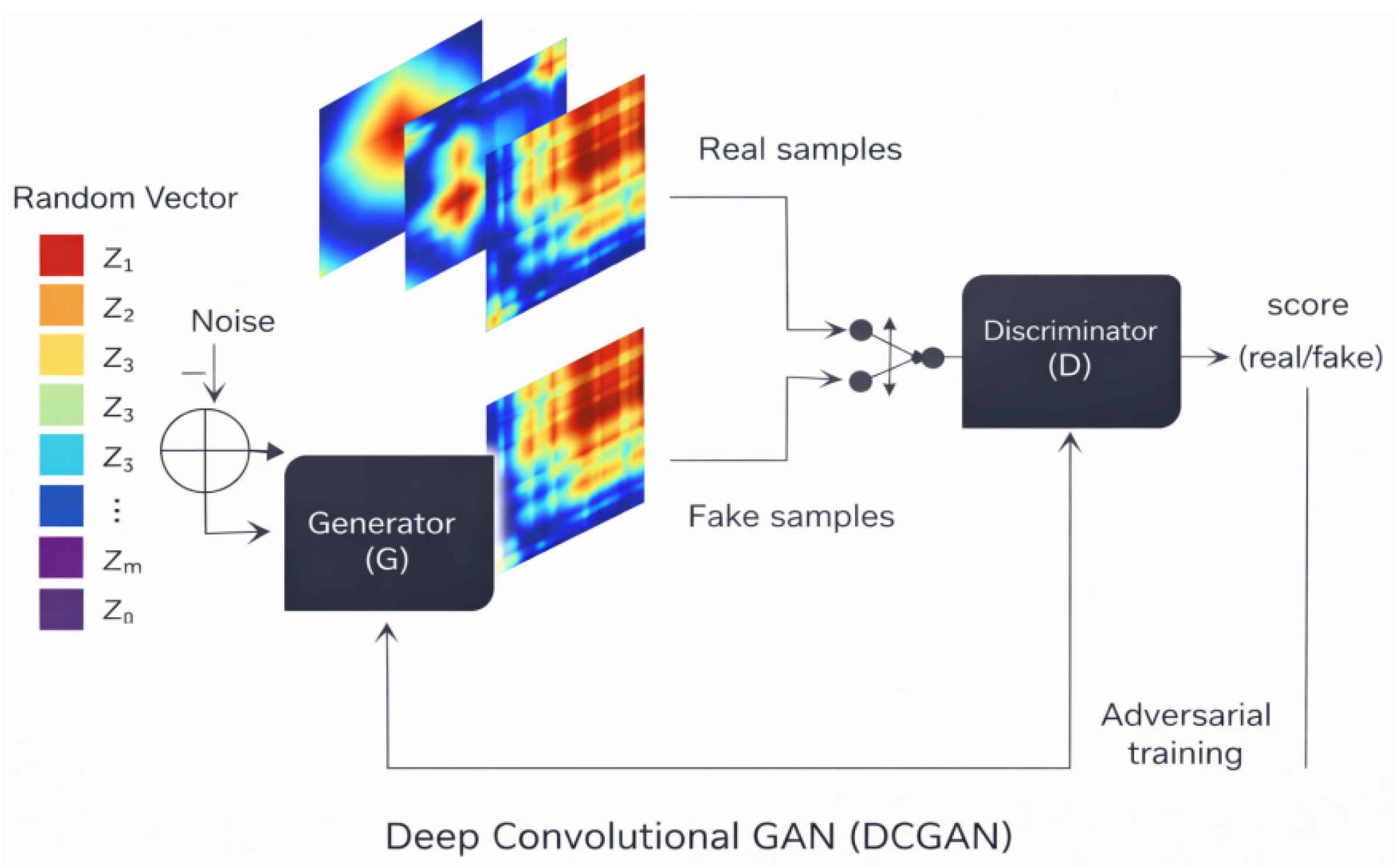
This work uses a deep convolutional generative adversarial network (DCGAN) to generate image samples from PV and wind datasets to increase data diversity and realism. DCGAN works in an adversarial way: the generator generates fake samples, and the discriminator learns to distinguish between real and fake samples, with competition while training. Such competition enables the model to learn important information of target data distribution and generate better synthetic samples even with limited real samples [42]. The overall workflow of the proposed DCGAN, including the generator, discriminator, and adversarial training process, is illustrated in Figure 3.
The generator starts from a 128-dimensional latent noise vector and upsamples it through deconvolution (ConvTranspose2d) layers. Batch normalization and ReLU activations are used to stabilize training and capture nonlinear features, and a final Tanh layer maps pixel values to [−1, 1]. The discriminator consists of stacked convolutional layers and employs LeakyReLU to mitigate vanishing gradients [43]. Its final Sigmoid layer outputs a probability score indicating whether an input sample is real or generated.
To rebalance the dataset, we employ a DCGAN with tailored generator and discriminator architectures. We adopt a composite objective to improve image quality and training stability, consisting of the standard adversarial loss, a gradient-penalty regularization term (as in WGAN-GP) to mitigate training instability and mode collapse [44], and an MSE-based pixel-level loss to match generated and real images [45]. During training, the generator and discriminator are updated alternately. After convergence, the resulting synthetic images are used to augment minority classes, yielding a more balanced dataset.
Figure 3.
Workflow of the deep convolutional generative adversarial network.
The DCGAN is trained only on real training samples. After training, the generated synthetic samples are mixed with the real samples to construct balanced training sets with total sizes of 1000, 2000, and 3000 samples. We build a DCGAN for generating PV and wind sample images separately. For PV, the balanced training set reaches 2000 samples after augmentation. The maximum iteration configurations are set as 20,000, which allows the model to train under complicated irradiance conditions. Other configurations are mostly the same as the wind task. We further set saving checkpoints and evaluating during training more frequent to enable online evaluation of generation quality in real time. For wind, the balanced training set reaches 3000 samples after augmentation. The model is trained for 20,000 iterations. We set batch size as 128 and learning rate of generator and discriminator as 2 × 10⁻⁴ and 4 × 10⁻⁵, respectively. We use Adam to update parameters with β1 = 0.5 and β2 = 0.999.
To keep training dynamically balanced, CosineAnnealingLR is adopted to update learning rates for both networks. This schedule gradually decays the learning rate over long runs, thus helping to limit overfitting and support stable convergence [46].
2.2.2. Quality Evaluation of Generated Samples
We use the Fréchet Inception Distance (FID) in [47] to measure the similarity between synthetic and real samples in PV and wind. During the training process, we output the synthetic samples at fixed epochs of 3000, 5000, 10,000, and 20,000, and save the model checkpoint simultaneously. We use the generator with the smallest FID as the optimal model. In Appendix A, we show the FID curves in different training ranges. We output the FID curves of 0–3000, 0–5000, 0–10,000, and 0–20,000 iterations of PV in Figure A1 and wind in Figure A2. Generally, a smaller FID represents better generation performance. In both datasets, FID decreases rapidly at the beginning, and then it becomes stable. This phenomenon indicates that adversarial training can reduce the gap between generated and real distribution. In PV, FID decreases most in the range between 1000 and 2000 iterations. Then, it stays at a low level. Usually, the best FID appears in the range between 5000 and 10,000 iterations. In wind, FID also decreases rapidly at the beginning, but then it fluctuates. This phenomenon may come from the more complex texture of image and operating condition. After 5000 iterations, FID stays in a low level with small fluctuation. Therefore, training 20,000 iterations can only bring small improvement. In this case, it is better to choose the model with smallest FID than to train more iterations.
FID is based on the pretrained feature extractor. So, its value may change when the data are far from the domain of the feature model. Therefore, we use FID as the main evaluation metric, but we do not rely on FID alone. We also check the sample image by visual inspection. Finally, we use the downstream task to test the data. These can make the evaluation more reliable. In both solar and wind, DCGAN reduces the gap between generated and real distribution during the training process. And then the FID curve reaches a stable plateau in the middle or later stage. We choose the model with smallest FID and use early stopping. Finally, these can provide synthetic samples which are close to real distribution. And then these can support the later state monitoring and performance evaluation.
3. System Description
3.1. Data Sources and Characteristics
Description of Raw Operational Data for PV and WP
The PV and wind datasets are collected from real power plant monitoring systems. For the PV dataset, 42 PV monitoring stations, deployed by La Trobe University at five campuses in Victoria, Australia, record the PV power output from January 2020 to December 2021, including 69,984 data points [48]. For the wind dataset, we use the public Longyuan wind operation dataset from the CSDN “China Software Cup” competition—provided by Longyuan Power Group, it includes the operation records of turbines from October 2020 to December 2022, including 78,912 data points [49]. Both datasets use a sampling interval of 15 min; each day is a sequence of 96 points (24 h × 4 samples per hour).
In Figure A3, we show some typical daily PV power curves in different operating states. Each state has different characteristics. When in a normal irradiance state (NI), the curve has a typical bell shape; it increases in the morning, reaches its peak around midday, and it decreases in the afternoon. The rise and fall are relatively symmetric. When in a weather-induced shading state (WIS), the curve shows large fluctuations around midday. There are sharp fluctuations or sudden drops around midday. The occurrence time of the sudden drop coincides with the moment of being occluded by clouds, snow, etc. When in an extreme temperature state (ETC), the maximum power is lower than in the NI state. This shows that high/low temperatures would affect the conversion efficiency, and the humidity effect is also considered. When in an equipment fault state (EF), the curve may suddenly break or have missing parts. It may indicate some problems with the inverter or sensor. When in a prolonged low irradiance state (PLIC), the curve stays at a low level during the whole day. It may coincide with the rainy season or long-term low irradiance.
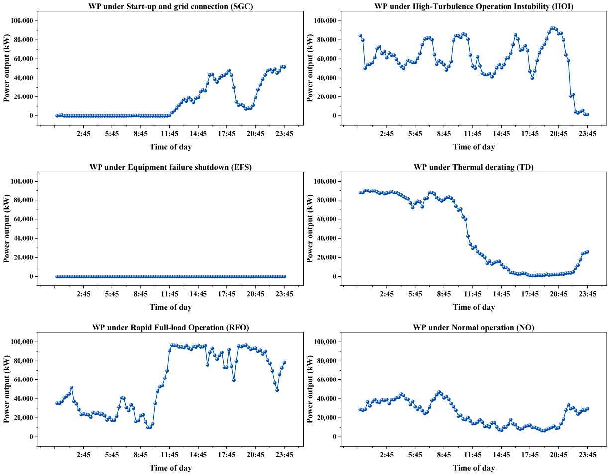
Figure A4 shows daily wind power curves for different operating states. (a) Normally operating power varies smoothly as a function of wind speed. The range of the values in this plot varies from near-partial load to near-rated operation for typical wind farms. (b) High-turbulence unstable operation (HOI) shows large fluctuations over a short period of time with recurring spikes (turbulence-driven instability). (c) Thermal derating (TD) shows a decrease in power during the hot daytime hours. The daily maximum is lower than in (a)—this is consistent with the temperature constraint of wind farm output. (d) Rapid full-power operation (RFO) shows a rapid increase from near zero to near rated power and then sustained at that level. This type of curve would be associated with a rapid change in wind speed to a high speed which maintains it above rated. (e) Fault shutdown (EFS) shows sustained operation at zero power for long periods, although there are some cases where the wind farm is observed to run for a period then drop to zero (this may indicate component faults or protection shutdowns). (f) Grid-connected start-up (SGC) shows a slower ramp up from zero to a medium-to-high range. The ramp-up includes recurring fluctuations. This type of curve is associated with the start-up from shutdown to grid-connected operation.
These operating states characterize typical wind-turbine behaviors under diverse wind and equipment conditions and provide necessary support for subsequent imbalance analysis and operating-state modeling.
3.2. Data-Processing Workflow
3.2.1. GASF-Based 2D Image Transformation from One-Dimensional Data
This study employs the Gramian Angular Summation Field (GASF) to transform one-dimensional PV and wind time-series signals into two-dimensional images [50]. Specifically, GASF maps a time series to a 2D matrix while preserving temporal ordering and encoding it into a structured spatial representation. This representation provides richer inputs for subsequent deep-learning models and facilitates feature learning [9].
- Data Normalization and Polar Coordinate Mapping
The raw time series is first normalized so that its values are scaled to the range [−1, 1]:
Among them, .
Next, we use a polar-coordinate transform. This step maps each normalized value, , to an angle.
Here, denotes the angle, is the normalized time step, and is the sequence length. With this mapping, the time series is represented as a trajectory in the angle–radius coordinate system.
- b.
- Gramian Angular Summation Field Construction
Subsequently, we construct the Gramian Angular Summation Field (GASF) matrix from the polar-coded values. Formally, it is defined as follows:
By taking the summed angles of any two time points, this matrix captures overall temporal dependence in the sequence. The symmetry of the cosine function allows to retain both the global trend and local dynamic characteristics of the time series.
- c.
- 2D Image Generation and Feature Representation
The resulting GASF matrix is fed into the model as a 2D image. Compared with the original 1D time-series input, this representation preserves amplitude information while encoding temporal correlations into an explicit geometric pattern [50]. Figure 4 illustrates the complete pipeline for converting PV and wind operational data into GASF images: the raw time series is first mapped via polar encoding and then transformed into a Gramian angular field image. As shown, the GASF image exhibits obvious 2D structural patterns, and these features can be extracted via convolutional neural networks for further classification.
Figure 4.
Conversion principle of time series into Gramian Angular Field (GASF) images via polar encoding.
Specifically, the raw one-dimensional time series is first normalized to the range [−1, 1], and each normalized value is then mapped to a polar coordinate, in which the angular coordinate encodes the value itself and the radial coordinate encodes its temporal position. The GASF matrix is obtained by computing, for every pair of time points, the cosine of the sum of their angular coordinates. In the resulting image, both the horizontal and vertical axes correspond to time, the main diagonal preserves the normalized values of the original series, and each off-diagonal element encodes the temporal correlation between the two corresponding time points through a color intensity. This transformation converts the dynamic behavior of PV and wind power signals into visible spatial textures—smooth gradients for stable operation and abrupt local variations for faults or weather-induced fluctuations—which are subsequently extracted by the CNN.
Figure 5 shows GASF images for PV data under several typical states. These states include NI, WIS, PLIC, ETC, and EF. The images show clear pattern differences across states. These differences reflect different dynamics in the original time series.
Figure 5.
Gramian Angular Field (GASF) images of PV time series under different operating conditions.
Figure 6 shows GASF images for wind data under NO, HOI, TD, RFO, EFS, and SGC. The spatial patterns also differ clearly across these states. Many states remain easy to separate based on image structure. Overall, GASF makes hidden time-series patterns more visible. It creates useful image inputs for later deep-learning models. This step supports state recognition and classification.
Figure 6.
Gramian Angular Field (GASF) images of WP time series under different operating conditions.
3.2.2. K-Means Clustering for State Label Generation
For PV and wind operating-state data, we collected 728 and 818 samples, respectively, and applied an improved K-means clustering method for automatic identification and classification of operating conditions. K-means seeks the optimal clustering by iteratively minimizing the within-cluster sum of squared errors [51], and its objective function is expressed as follows:
Here, k is the number of clusters, Ci denotes the sample set in the i-th cluster, and is the centroid of that cluster [52].
To handle complex energy data more reliably, we modify the standard K-means method. We add two components: feature weighting and trimmed-centroid updates [53]. The feature-weighting step assigns an adaptive weight to each feature. It compares how well the feature separates classes with how much it varies within each class. We compute the weight as the ratio of inter-class dispersion to intra-class dispersion, as follows:
Here, is the weight of the d-th feature; denote the between-class and within-class dispersion of the d-th feature, respectively; and D is the feature dimension. This mechanism emphasizes informative operational features while suppressing noisy dimensions. Meanwhile, during centroid updates, only the closest p% (e.g., 90%) values of samples within each cluster are used to recompute the centroid, expressed as follows:
Here, denotes the set of the closest p% samples in cluster i. By combining feature weighting and the trimmed strategy, this method reduces the influence of outliers on clustering convergence, improving stability and interpretability under the high variability and strong noise typical of renewable energy systems.
To further verify the effectiveness of the proposed features and clustering approach, t-distributed stochastic neighbor embedding (t-SNE) is used to project high-dimensional features into a 2D space for visualization [53]. By preserving neighborhood similarity as much as possible during the mapping, t-SNE makes the clustering and separation of different conditions/classes more visible in the 2D plane, providing intuitive evidence for feature separability and clustering validity [54]. As shown in Figure 7, PV time series are grouped into five clusters (C0–C4), covering WIS, EF, PLIC, NI, and ETC. As shown in Figure 8, WP time series are grouped into six clusters (C0–C5), corresponding to RFO, HOI, EFS, SGC, TD, and NO.
Figure 7.
t-SNE visualization of clustering results for photovoltaic (PV) operating states, showing five distinct clusters (C0–C4).
Figure 8.
t-SNE visualization of clustering results for wind power (WP) operating states, showing six distinct clusters (C0–C5).
The t-SNE visualization shows that most clusters are reasonably well separated, suggesting that the learned features capture pertinent differences in the time-series patterns. Samples are tightly grouped within each cluster, while different clusters remain clearly separated. These observations provide qualitative evidence for the effectiveness of the proposed K-means variant with feature weighting and trimmed-centroid updates in identifying typical operating modes in renewable energy systems.
3.2.3. Verification of Pseudo-Labels Against SCADA Records and Centroid-Distance Filtering
The K-means variant assigns labels without supervision, so two safeguards were applied before any pseudo-label was used for CNN training: a sample-based verification against the SCADA records of the corresponding plants, and the removal of samples whose cluster membership was ambiguous. The number of samples involved and the criterion applied are stated explicitly below and in Table 1.
Table 1.
Per-cluster training samples, centroid-distance exclusion, and SCADA verification.
Verification against SCADA records. Pseudo-labels were generated by the K-means variant on all 1546 daily samples (728 PV and 818 wind) before the 64/16/20 split of Section 4.1; the split was applied afterward, and no test sample was used at any stage of CNN training or data augmentation. From the clustered samples, a stratified random subset was drawn for manual verification, with 7.1% of the samples of each cluster selected at random and a minimum of four samples per cluster. The subset contains 110 samples in total (52 PV and 58 wind), i.e., 7.1% of the 1546 clustered samples. Each sample was aligned in time with the SCADA entry at the beginning of its 96-point daily window and compared with the state recorded there: for the wind turbines, the recorded power, wind speed, pitch angle, generator speed, and alarm code; for the PV stations, the inverter status, availability, and maintenance records. The check found no cluster whose labels were systematically in conflict with the SCADA records; the only discrepancies concerned the boundary between thermal derating (TD) and the partial-load segment of normal operation (NO) in the wind subset, and none of them required a cluster to be relabeled. The per-cluster distribution of the verified samples is given in Table 1. Because the check served to validate labels only, the verified samples were not removed from the training data.
Centroid-distance filtering. Distances were measured in the same feature space in which the clustering was performed, namely the weighted, z-score-normalized feature, vector xi ∈ RD, and not on the GASF images. For sample i in cluster Ck with centroid ck, the distance is
and the acceptance threshold was computed separately for every cluster as the 90th percentile of the distances of that cluster’s training samples,
A training sample was excluded when di > τk, i.e., when it fell in the farthest 10% of its own cluster. Because the threshold is defined per cluster, the rule removes 10% of each cluster rather than 10% of the dataset as a whole. The filter acted on the training partition only: validation and test samples were never filtered and kept their SCADA labels. Table 1 reports, for each cluster, the number of training samples, the number excluded and the number retained; in total, 99 of the 989 training samples (10.0%) were excluded, leaving 890 for training. Since the filter acts on the training partition alone, it does not bias the reported test metrics, which are computed on unfiltered, SCADA-labelled samples.
4. Research Methodology
4.1. 2D-CNN Experimental Model Setup
4.1.1. Dataset Partitioning (Training/Validation/Test)
We represent operating-state signals as Gramian Angular Field (GAF) images, which are then processed by a convolutional neural network (CNN) to extract deep features. The dataset comprises 11 operational states spanning both PV and wind systems: five PV states (NI, WIS, ETC, EF, and PLIC) and six wind states (NO, HOI, TD, RFO, EFS, and SGC). For reproducibility, the data are split into training/validation/testing sets with proportions of 64%/16%/20%, using stratified sampling to preserve the overall class distribution in each subset. No DCGAN-synthesized samples were incorporated into the test set; the test set consists exclusively of real SCADA-recorded samples, and its labels were taken from the SCADA records rather than from the clustering output. The larger sample counts shown in the confusion matrices arise because each subplot corresponds to an independent experimental run under different data augmentation settings, where the total sample number represents the sum of predictions for that separate experiment rather than a single shared test set.
It should be clarified that the PV–wind combined scenario in this study integrates time-series samples collected from independent photovoltaic and wind power plants, rather than synchronized co-generation measurements from a single hybrid PV–wind farm. The data integration strategy mixes individual samples of PV operating states and wind operating states within one unified dataset, without requiring time-synchronized coupled power output of PV and wind. This multi-state mixed dataset enables the model to learn the characteristic patterns and fault signatures of both PV and wind equipment simultaneously. The proposed framework is therefore applicable to multi-source renewable energy systems, and can be further extended to analyze time-aligned coordinated operating data of hybrid PV–wind plants in future work.
4.1.2. 2D-CNN Model Structure and Training Parameters
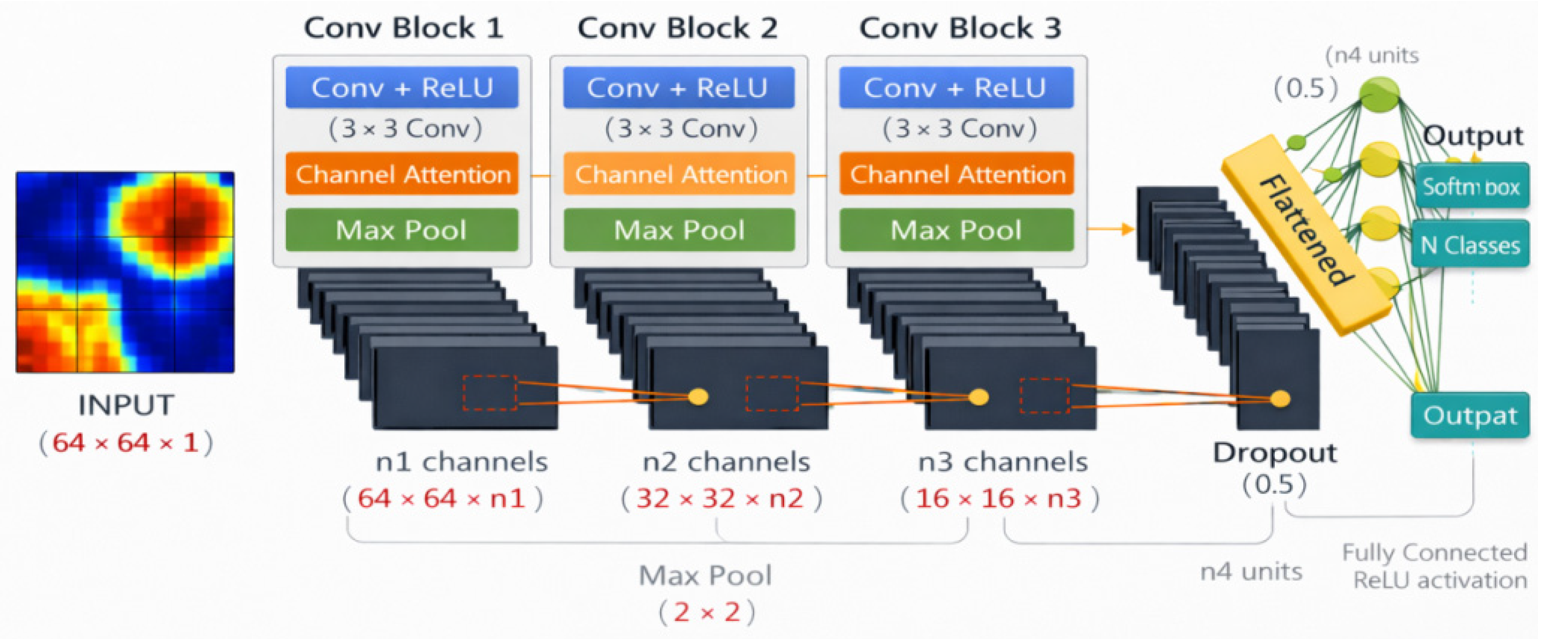
Figure 9 illustrates the architecture of the 2D-CNN with channel attention. In the model design, channel attention is introduced into the convolutional blocks of the improved CNN to reweight and recalibrate feature-map channels, encouraging the network to emphasize informative channel features and improve discriminability [55]. Dropout regularization is also used to suppress overfitting. For ResNet-34, the input layer is adjusted, and the initial pooling layer is removed to accommodate 64 × 64 inputs; a Dropout layer is inserted before the fully connected layer to enhance generalization [56].
We train the model with a batch size of 128 for a maximum of 100 epochs. AdamW is used as the optimizer, with an initial learning rate of 1 × 10⁻³ and a weight decay of 1 × 10⁻⁵ [57], and cosine annealing is applied for learning-rate scheduling. To accelerate training, we incorporate mixed-precision training and multi-GPU data parallelism. Random seeds are set to ensure result consistency. Mixed-precision training reduces memory consumption and boosts training speed without compromising accuracy [58]. All data processing, GAF transformation, GAN augmentation, and CNN modeling in this study were implemented using Python 3.9. The deep-learning framework PyTorch 1.12 was adopted for model construction and training. Scikit-learn 1.1.3 was used for dataset partitioning and evaluation metric calculation. Pandas 1.4.4 and NumPy 1.22.4 were utilized for SCADA data loading and numerical computation. Matplotlib 3.5.2 was used to generate intermediate visualization figures, while OriginPro 2023 was employed to plot the final result figures in this manuscript.
Figure 9.
Architecture of the 2D-CNN with Channel Attention Module for image classification. The model incorporates convolutional blocks with integrated attention, dropout regularization, and fully connected layers to enhance feature selection and generalization.
4.2. Performance Evaluation Metrics
Accuracy, Macro-F1, Weighted-F1, Min-F1, and Confusion Matrix
We evaluate the model using multiple metrics, including accuracy, Macro-F1, Weighted-F1, the minimum per-class F1 (Min-F1), and the confusion matrix. These metrics summarize overall performance while enabling class-wise analysis via confusion-matrix visualization and per-class accuracy, which facilitates comparisons between majority and minority classes. Min-F1 is reported as a worst-case indicator, corresponding to the most challenging class. Precision, recall, and F1 are computed from the confusion matrix [59]. We additionally report ROC and precision–recall (PR) curves with per-class AUC and average precision (AP). Under pronounced class imbalance, PR curves are typically more informative than ROC curves for assessing practical performance [60] and for examining robustness across decision thresholds.
5. Results and Discussion
5.1. Recognition Performance Under Imbalanced Data
2D-CNN Result Comparison Across All Scenarios
As shown in Figure 10, under imbalanced training, the 2D-CNN exhibits clear differences in overall performance and class-level behavior across the three scenarios.
Figure 10.
Comprehensive evaluation of the 2D-CNN across PV, wind, and hybrid scenarios under imbalanced data. Model performance is compared using accuracy, Macro-F1, Weighted-F1, and Min-F1 metrics.
In the PV scenario, the model nears its performance upper limit, delivering an accuracy of 95.89%, a Macro-F1 of 95.62%, a Weighted-F1 of 95.89%, and a minimum F1-score (Min-F1) of 94.12%. These outcomes attest to stable performance across all classes under mild class imbalance conditions. In the wind scenario, despite a comparable imbalance ratio, the Min-F1 plummets to 44.07%, with accuracy and F1 scores also dropping to roughly 58–60%. This discrepancy highlights that the imbalance ratio alone cannot adequately explain task complexity; class separability and the quality of long-tail samples are likely the key contributors to the observed performance degradation. In the combined PV–wind scenario, the imbalance ratio increases to 4.186, denoting more severe class imbalance. Nevertheless, the expanded dataset scale and enhanced separability of specific classes elevate the overall accuracy and Macro-F1 to approximately 82%. However, the Min-F1 remains merely 46.15%—far below the PV scenario’s result—underscoring that imbalance and inter-class confusion still impede the recognition of tail classes. Collectively, Macro-F1 and Min-F1 act as core metrics for assessing 2D-CNN performance under imbalanced conditions. Macro-F1 mirrors the balance of performance across classes, while Min-F1 establishes a lower bound for the most challenging class. By analyzing these two metrics in conjunction with the imbalance ratio, we obtain a deeper insight into how class imbalance affects operating-state recognition in renewable energy systems.
In the PV scenario shown in Figure 11, the 2D-CNN training and validation losses drop rapidly in the early stage and quickly stabilize, while their gap remains small over time, indicating smooth convergence and a low risk of overfitting. Meanwhile, validation accuracy and F1 rise quickly and stay above 0.90; together with the classification report (Macro-F1 ≈ 0.96 and the lowest class-level F1 still ≈ 0.92), this suggests that class imbalance in this scenario is relatively manageable and within-class features are more concentrated, enabling the model to learn more discriminative representations and achieve good inter-class separation.
Figure 11.
Training and validation curves (accuracy/loss) for the deep-learning model trained on imbalanced photovoltaic data.
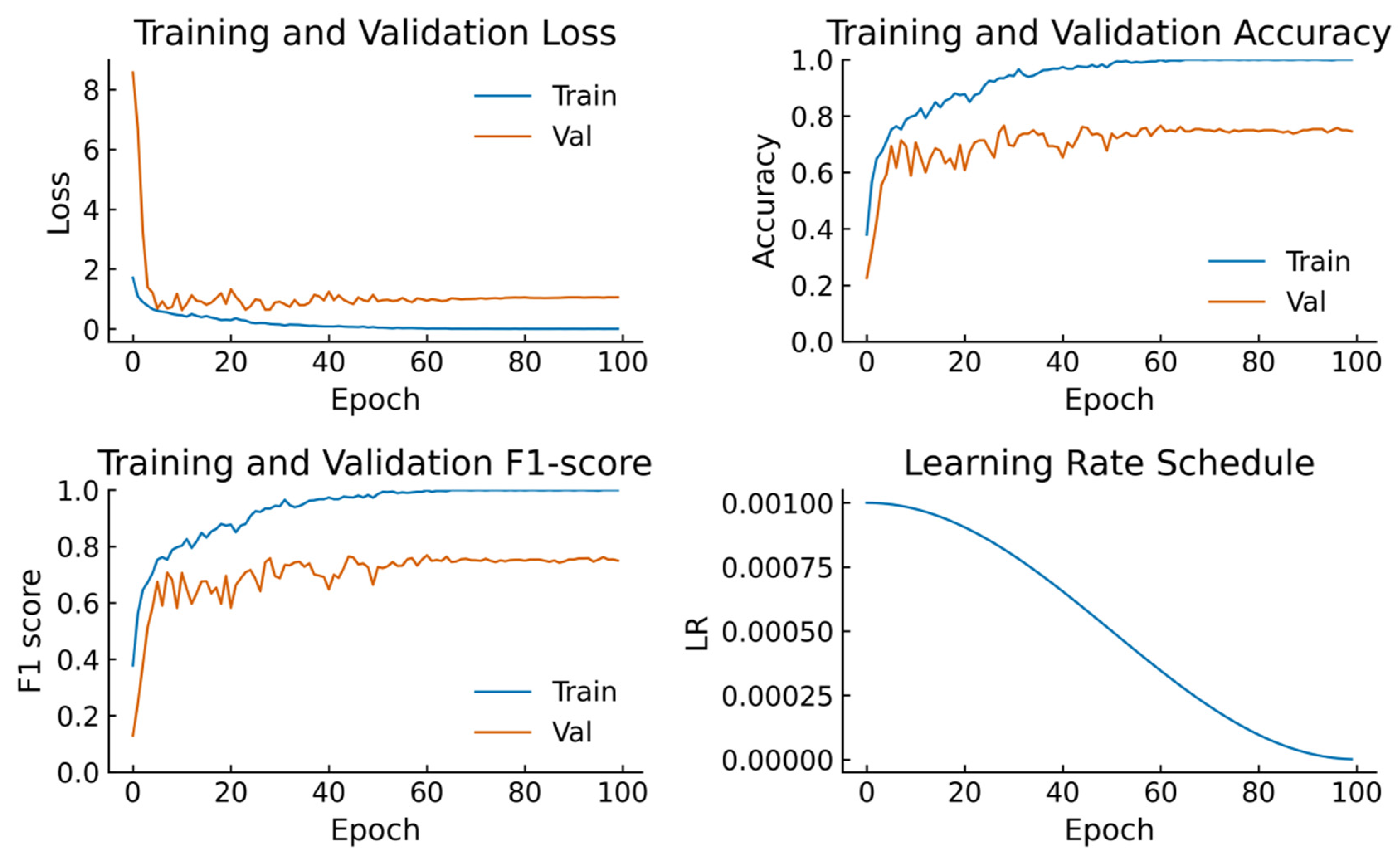
Compared with the wind single-scenario results in Appendix B (Figure A5), the wind training loss keeps decreasing and training accuracy rises steadily, yet validation accuracy fluctuates in the 0.60–0.70 range for a long period. The validation F1 is clearly lower than accuracy and oscillates around ~0.60, indicating more severe tail-class recall shortage and inter-class confusion under a long-tail distribution; the worst-class F1 is only ~0.32, further showing that minority classes fail to form stable decision boundaries. In Figure A6, cross-scenario fusion training still converges stably and, relative to the wind-only setting, notably improves validation performance, stabilizing both accuracy and F1 at around ~0.75; overall accuracy, Weighted-F1, and Macro-F1 in the classification report (≈0.82–0.83) also improve. This suggests that cross-domain data fusion strengthens discriminative feature learning and partially mitigates the wind long-tail effect, yet learning remains insufficient for extremely scarce classes, implying that simply stacking cross-domain data cannot fully resolve recognition difficulties caused by class imbalance.
The confusion matrices indicate that class separability varies depending on the circumstances. Their patterns of confusion are also different. The model classifies most of the samples in the PV scenario (Figure 12). A majority of the errors remain in few near classes. The model is, however, at times, confused when it comes to equip equipment fault and extreme temperature. It also at times mixes shading by weather conditions with long periods of low irradiance. The matrix is almost perfect in general. This trend implies that PV classes are small in nature and their boundaries are definite. The confusion is stronger in the wind scenario (Figure 13). Connections between the model and grid connection and thermal derating are commonly mixed up. It is also confused with high turbulent instability and operating normally. These flaws bring about obvious cross-class leakage. This outcome is associated with two aspects. One, the wind data are not normally distributed. Second, there are similar patterns of features in some wind states. Although high accuracy of some head classes may not deteriorate performance, low recall of tail classes may still lower the overall performance.
Figure 12.
Confusion matrix of the 2D-CNN classifier on photovoltaic data under the imbalanced training setting.
Figure 13.
Confusion matrix of the 2D-CNN classifier on wind power data under the imbalanced training setting.
The confusion matrix on the PV–wind situation (Figure 14) has a more balanced distribution. Most classes have higher values on the diagonal, an adjustment that suggests that the incorporation of data on solar energy (PV) and wind makes the model more likely to recognize a minority condition of wind than the situation when using wind alone. An example is that the model consists of increased correct classification rates of TD and SGC samples, whereas the confusion between NO and HOI is reduced to some extent. However, scattered misclassification errors are observed in certain tail classes, yet this trend underscores the fragility of this approach in terms of class imbalance and sample insufficiency as major limitations to future performance enhancement.
Figure 14.
Confusion matrix for the 2D-CNN classifier on combined photovoltaic and wind power data.
Class imbalance is one of the key factors that lead to the decrease in performance, and the effect is likely to become stronger when several scenarios have to be considered. To address this problem, later experiments use DCGAN to add tail classes in a specifically directed way, so as to readjust the distribution of classes and improve the separability of minority classes. We confirm the improvements obtained by tracking the improvement in Macro-F1 and the minimum class-level F1.
5.2. Recognition Performance Under Balanced Data
5.2.1. PV Scenario Results and Improvement Magnitude
In the PV scenario, we further compare how balanced datasets of different sizes affect 2D-CNN performance (Figure 15). Overall, as the balanced dataset grows, the model shows consistent gains in accuracy, Macro/Weighted-F1, and minimum class-level F1. The steady increase in Min-F1 is particularly important, indicating that the improvement is not merely driven by head classes but reflects a real enhancement in tail-class discriminability. This result also supports that DCGAN-based targeted generation and rebalancing can reduce bias introduced by class imbalance and, with larger balanced datasets, further raise the model’s performance ceiling.
The confusion matrix in Figure 16 further supports the conclusion at the class level: as the size of the balanced dataset increases, misclassification patterns continue to converge, and inter-class confusion is markedly reduced, with the improvement mainly reflected in fewer errors for minority classes. Under the large-scale balancing setting, predictions become strongly diagonal-dominant, indicating that DCGAN-generated synthetic samples help stabilize decision boundaries for minority classes and, on this basis, achieve a more balanced classification performance.
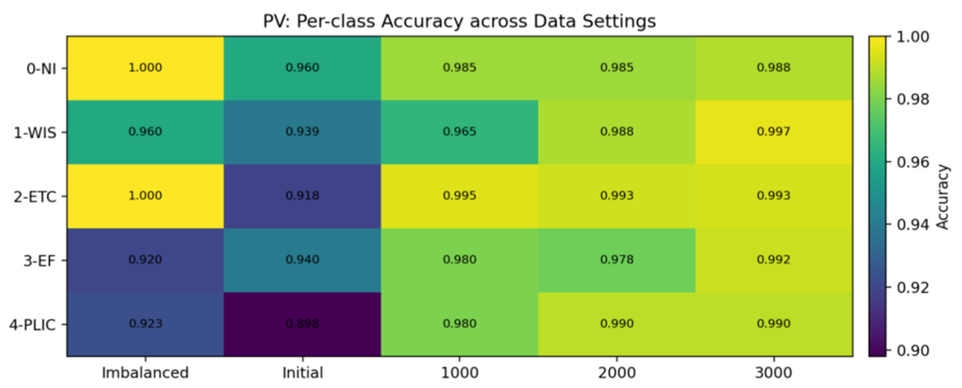
Figure 17 further illustrates, at the class level, how different data settings affect the prediction stability of the PV method. Under the imbalanced dataset, head classes already achieve near-saturated accuracy, while minority classes show a clear performance collapse in the “initial” setting, reflecting the direct impact of distribution bias on disadvantaged classes. When the balanced dataset size increases to 1000 or above, class-wise accuracies recover overall and become more consistent, indicating that rebalancing leads to more even performance across classes; the “initial-setting trough” is effectively corrected, and the separability and prediction reliability of minority classes are substantially improved.
Figure 15.
Performance comparison of 2D-CNN under different balanced distributions in photovoltaic scenarios.
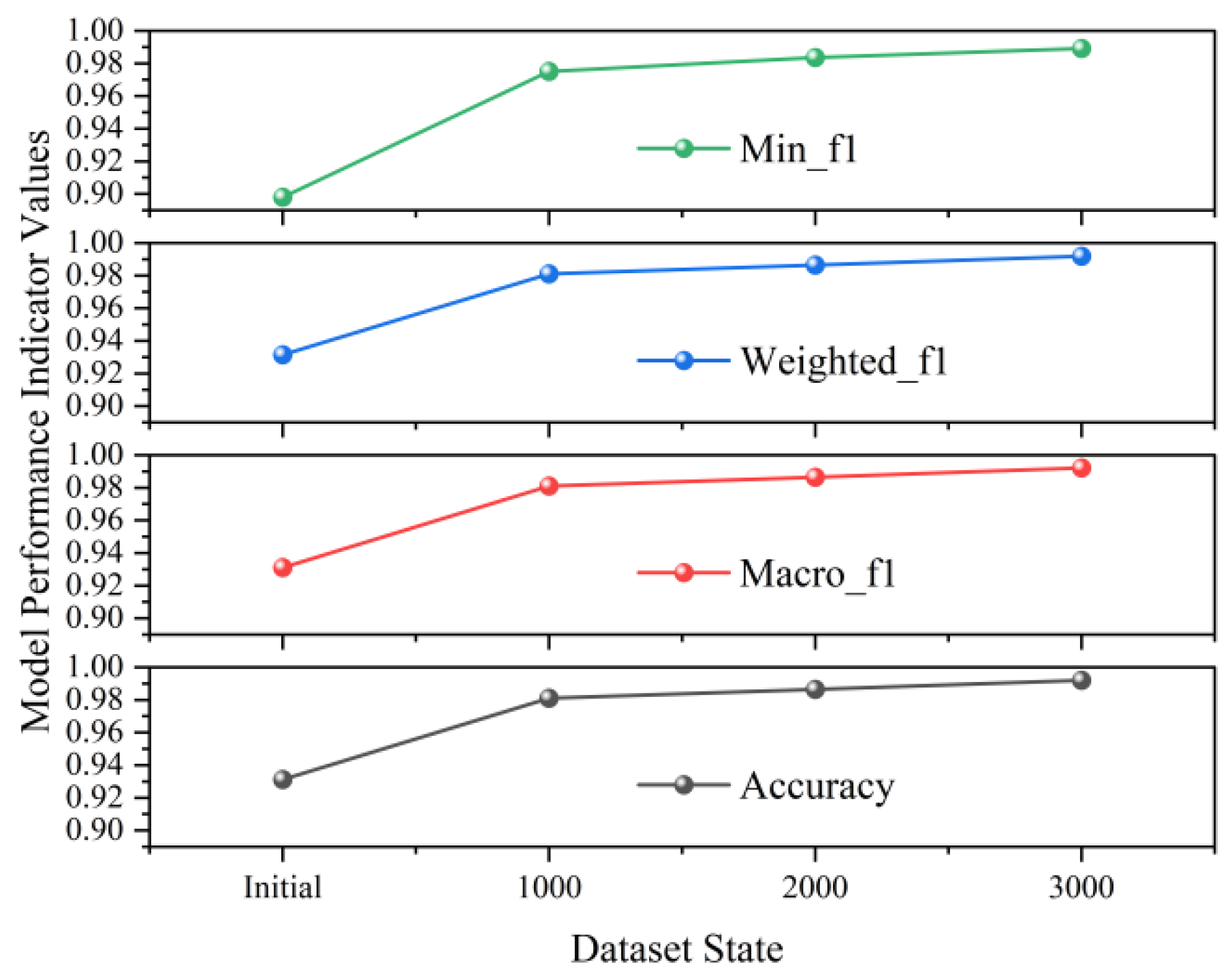
Figure 16.
Confusion matrix for the 2D-CNN classifier on photovoltaic data.
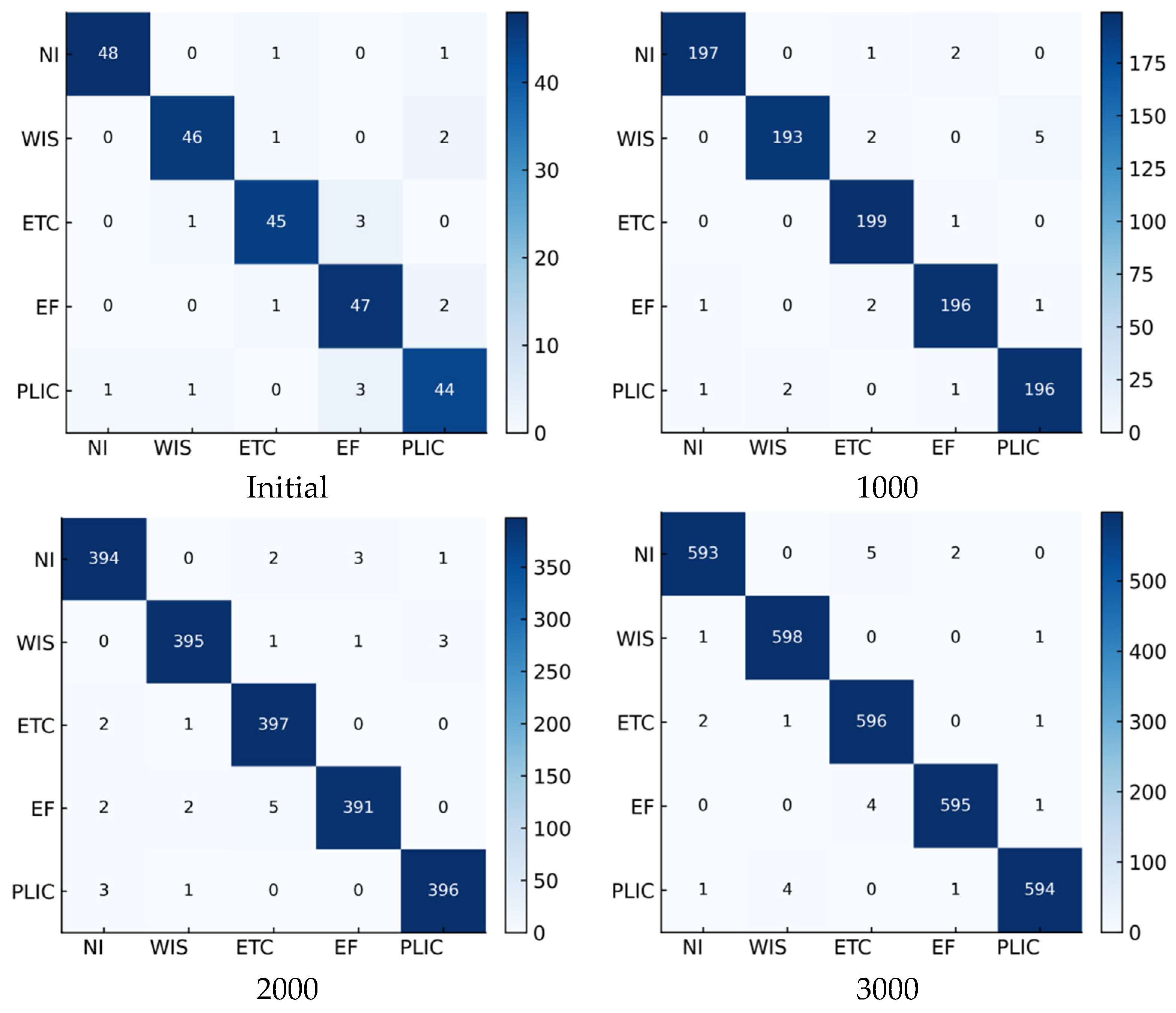
Figure 17.
Per-class accuracy of the 2D-CNN model under different data settings in the PV scenario.
5.2.2. WP Scenario Results and Improvement Magnitude
Figure 18 shows how different balanced dataset sizes affect the 2D-CNN in the wind setting. The trend is clear. As we increase the balanced dataset size from the initial level, performance improves in a steady way. Accuracy rises. Macro-F1 and Weighted-F1 also rise. The biggest gain appears in the minimum class-level F1. These results suggest two points. Rebalancing improves overall metrics. More importantly, it helps the model learn tail classes. It also makes their decision boundaries more stable. In this way, rebalancing reduces the main generalization limit caused by the long-tail distribution in the wind dataset.
Figure 18.
Performance comparison of 2D-CNN under different balanced distributions in wind power scenarios.
Figure 19, together with the confusion matrices, confirms the effectiveness of the rebalancing strategy in the wind scenario. In the initial setting, the diagonal is not sufficiently dominant, and cross-class confusion is widespread; several disadvantaged classes are also more likely to be misassigned to other classes, reflecting unstable decision boundaries under a long-tail distribution. As the balanced dataset expands, the diagonal gradually strengthens, off-diagonal errors converge markedly, and the classes that were previously most confused become more clearly separable. This indicates that, after adding synthetic samples and rebalancing, the model’s cross-class prediction distribution becomes more consistent, recognition reliability for tail classes improves in a substantive way, and overall performance is enhanced accordingly.
Figure 19.
Confusion matrix for the 2D-CNN classifier on wind power data.
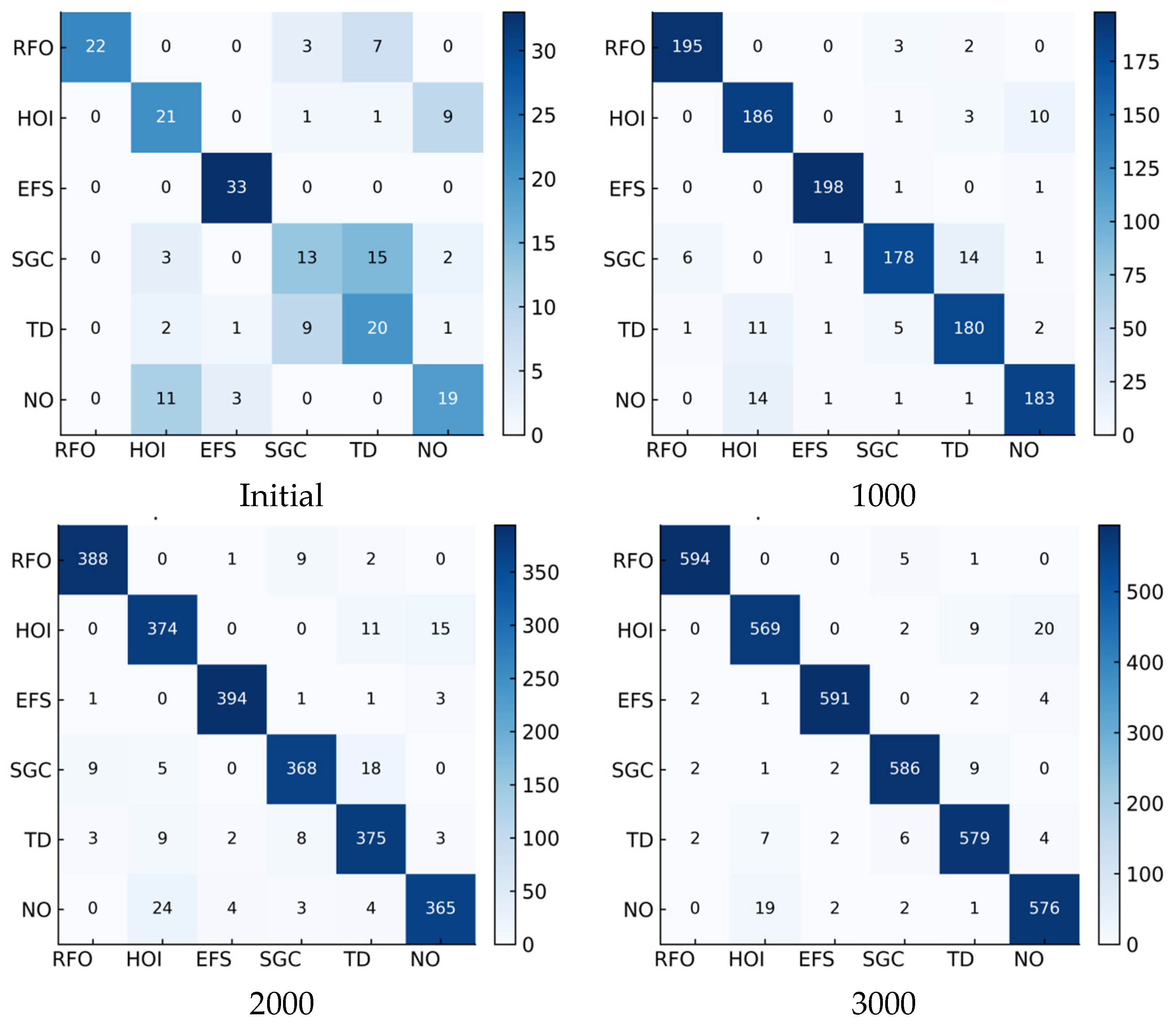
Figure 20 shows another benefit of rebalancing in terms of class-wise accuracy. Originally, in the imbalanced setting, most class accuracies are low and vary a lot from class to class. Applying larger balanced datasets (up to 1000 samples and beyond) results in improved class accuracies for most classes and an increased similarity between classes (more stability). This observation correlates with the improvements for the overall metrics and confusion matrices. We want to show that by an optimization of the data, the long tail is also suppressed in the wind scenario. Thus, the classifier is improved over all classes and not only the head classes.
Figure 20.
Per-class accuracy of the 2D-CNN model under different data settings in the WP scenario.
5.2.3. Combined PV–WP Scenario Results and Improvement Magnitude
Figure 21 shows that, in the combined PV–WP scenario, the 2D-CNN is still constrained by minority classes under the initial balancing setting, with a clearly low Min-F1. This suggests that higher class complexity and the long-tail effect in cross-scenario tasks amplify learning difficulty for tail classes. As the balanced dataset size increases, accuracy, Macro/Weighted-F1, and Min-F1 all rise in parallel, and the marked improvement in Min-F1 indicates that the gains mainly come from stronger recognition of disadvantaged classes rather than from majority classes alone. These results suggest that more sufficient balanced samples can improve generalization and class consistency in the combined scenario and, to some extent, mitigate insufficient recognition of minority classes.
Figure 21.
Performance comparison of 2D-CNN under different balanced distributions in photovoltaic and wind power scenarios.
Figure 22 shows the rebalancing effectiveness validity in the combined scenario; we use confusion matrices to show the rebalancing. In the first scenario, we can see that there are some classes that do not have a stable decision boundary; in the diagonal, there is not enough intensity, and more confusion in cross-scenario/cross-class is obvious. With the balanced-part size increase, the diagonal becomes more obvious, and the off-diagonal error decreases sharply; this result shows that the class separability is improved and the predictability of all classes becomes more consistent, and, at the same time, the tail-class performance is improved, and stabler, more correct recognition in tail-classes when rebalancing on a large scale is achieved. Therefore, the results show that our data augmentation and rebalancing scheme can effectively alleviate long-tail bias in multi-source data and improve the reliability of final classification results.
Figure 22.
Confusion matrix for the 2D-CNN classifier on combined PV and wind power data.
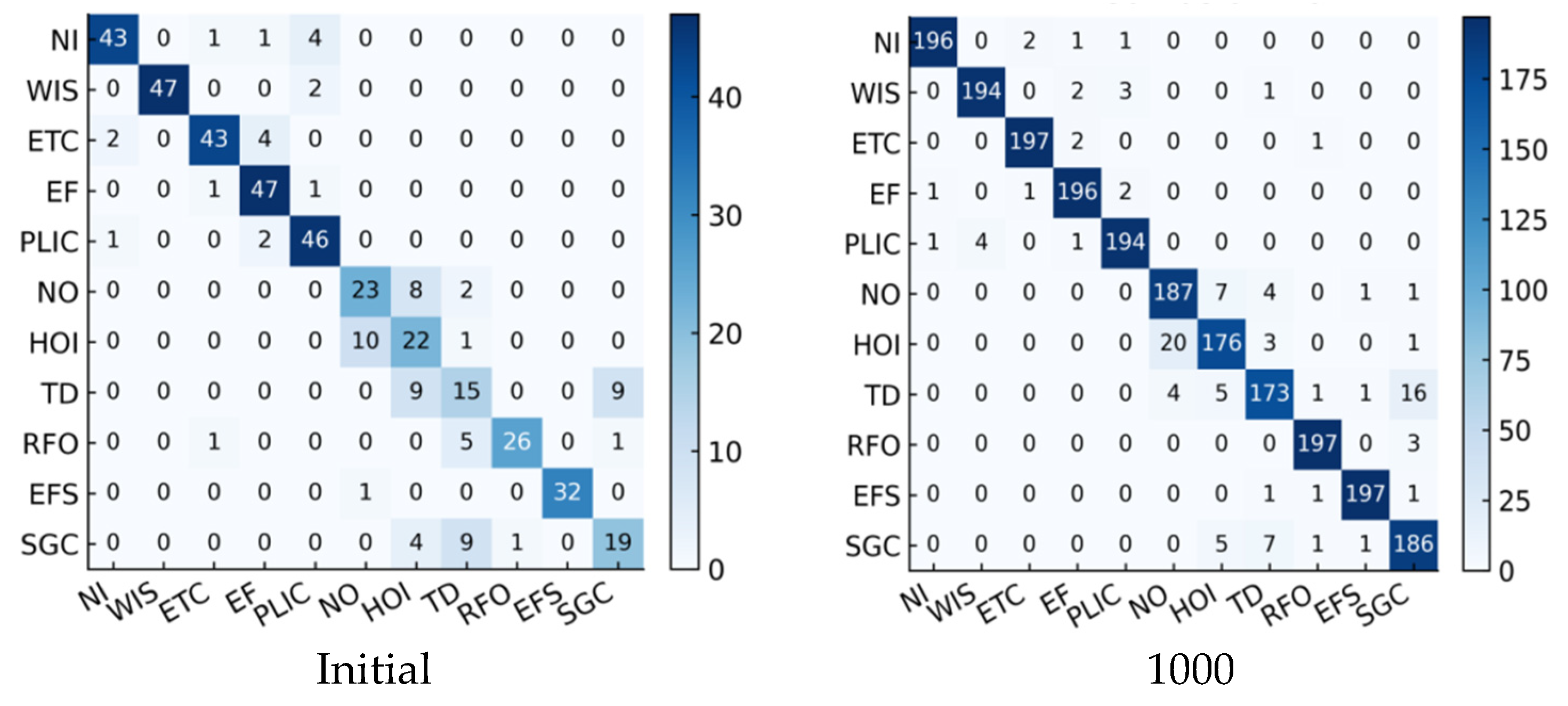
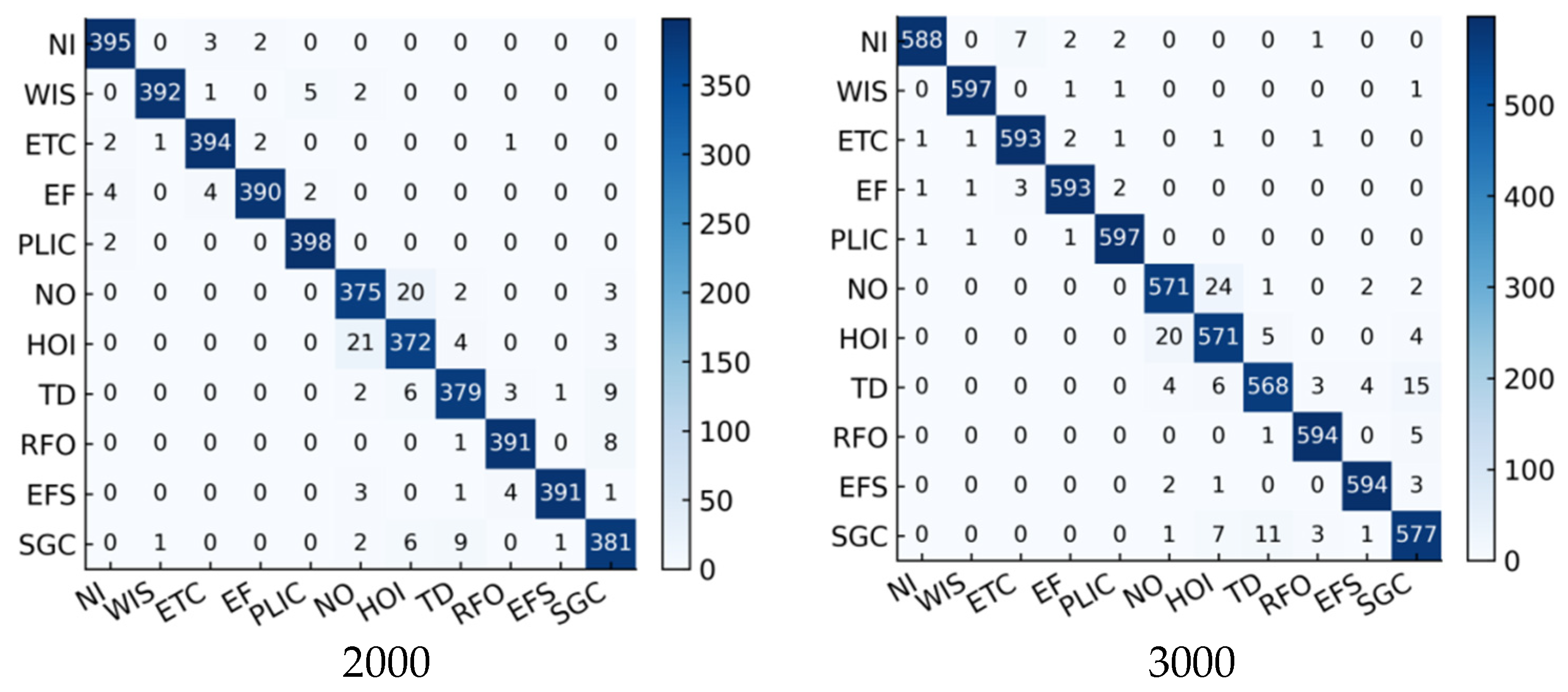
Figure 23 shows the impact of different data settings on prediction consistency in combined PV–WP. Class-wise accuracy is visualized in spatial distribution. In the imbalanced setting and initial balancing stage, class accuracies vary a lot: head classes are close to saturated accuracy, while tail classes remain much lower. This result illustrates that class imbalance in cross-scenario tasks will result in non-uniform gains over classes. When the balanced dataset size increases to 1000 and further, class accuracies increase in general and become closer to each other. The largest gain is obtained by weaker classes, and thus the gaps between classes become smaller. These results indicate that, compared to simply raising overall accuracy, rebalancing with synthetic samples also brings more advantages to multi-class prediction in the combined setting, i.e., better balance and stability, thus enhancing model reliability for integrated PV–WP tasks.
Figure 23.
Per-class accuracy of the 2D-CNN model under different data settings in the combined PV and wind power scenario.
5.3. Comparative Analysis and Discussion
5.3.1. Accuracy Difference Before and After Balancing
Converting microsamples to 2D images is a process that does not lose the important structural information on the signals. Then, we assign operating-state labels using K-means clustering, use DCGAN to obtain extra samples of the minority classes, and the synthetic samples are used to build a fairer training set. We compare the results of the 2D-CNN and rebalancing of the dataset, respectively, in terms of accuracy and other fundamental parameters of the scenario PV, wind, and the combined scenario. This comparative analysis makes it possible to measure the effectiveness of the rebalancing plan and confirm the main statement put across in the abstract, that there is stronger minority-class recognition and strong recognition of the operating state, as there is a balanced dataset. After establishing this effect of rebalancing, we repeat more experiments with balanced dataset sizes, leading to the outcome of the first rebalancing step, and, at the same time, balanced dataset sizes of 1000, 2000, and 3000. The configurations are evaluated relative to the original imbalanced dataset, and, in particular, the two important indicators are Macro-F1, which analyzes the multi-class performance, and minimum F1 (Min-F1), which measures performance gains of the poorest class.
Figure 24 shows slight negative deviations in ΔMacro-F1 at the initial stage of rebalancing for the PV-only and combined scenarios, indicating limited early improvement. In the wind-only setting, the gain is marginal (ΔMacro-F1 = 0.05), which is consistent with our previous finding that a limited number of synthetic samples is insufficient to fully counteract distribution-induced bias. As the balanced dataset size increases to 1000, 2000, and 3000 samples, ΔMacro-F1 improves across all scenarios. The wind-only scenario achieves the largest gain, reaching 0.37 at 3000 samples, whereas the combined and PV-only scenarios increase by 0.15 and 0.02–0.04, respectively. This further supports that wind data, characterized by more severe class imbalance, benefit more from rebalancing.
Figure 24.
Performance gains in Macro-F1 (Δ) of the 2D-CNN model over an imbalanced baseline for three power generation scenarios under various data settings.
The ΔMin-F1 results in Figure 25 further suggest that rebalancing yields the largest gains for minority classes. At the initial stage, improvements remain modest (PV, −0.04; wind, +0.08; and combined, −0.02). As the balanced dataset size increases, the gains become substantially more pronounced, with ΔMin-F1 rising to 0.59 in the wind scenario and to 0.46 in the combined scenario. These findings lend support to the conclusion stated in the abstract that balanced datasets improve the robustness of minority-class recognition. They are also consistent with the rationale that DCGAN-generated synthetic samples enhance the feature representation of minority classes, reducing the likelihood that these classes are overlooked or underrepresented.
Figure 25.
Performance gains in Min-F1 (Δ) of the 2D-CNN model over an imbalanced baseline for three power generation scenarios under various data settings.
Overall, the proposed DCGAN-based augmentation and rebalancing strategy improves both overall classification performance and minority-class recognition across the PV-only, wind-only, and combined scenarios. These results support the central conclusion that mitigating class imbalance enhances operating-state recognition in renewable energy systems. The method also demonstrates strong cross-scenario generalizability, providing a practical solution for data-driven operational monitoring.
The proposed framework integrates existing mature modules to tackle the multi-class imbalance fault diagnosis task for mixed PV–wind systems, whose novelty lies in the customized pipeline adapted for multi-source renewable operating state identification. Comprehensive comparisons with conventional oversampling strategies, class-weighted learning schemes, and alternative generative models, as well as systematic ablation studies, will be investigated in our future work to further validate the performance advantage of the proposed method.
5.3.2. DCGAN’s Impact on Minority Class Recognition
DCGAN can markedly improve minority-class recognition because the synthetic samples fill gaps in the minority feature space. Under the original imbalanced datasets, minority samples are scarce in the PV, wind, and combined PV–wind scenarios: the initial Min-F1 is only 0.4407 for wind (3-SGC accuracy < 0.4), 0.8980 for PV (1-WIS shows limited misclassification), and 0.4615 for the combined scenario (cross-scenario misclassification is prominent). By learning the feature distribution of minority-class GASF images and generating valid samples, DCGAN builds a balanced dataset together with real samples, which alleviates the model’s under-learning issue.
Quantitative results confirm the practical utility of DCGAN. The wind Min-F1 increases from 0.4407 to 0.9507 at the 3000 scale (peak ΔMin-F1 = 0.59), and the combined scenario rises from 0.4615 to 0.9438 (ΔMin-F1 = 0.46). Confusion matrices show that the correct count for wind 3-SGC increases from 13 to 586, and PV 1-WIS increases from 47 to 597 (diagonal proportion > 99%). This shift breaks the training dominance of majority-class features and improves minority-class accuracy and robustness.
Overall, DCGAN follows a clear logic of “supplement minority features → mitigate class imbalance → guide more even learning,” addressing the core difficulty of minority recognition. With wind and combined Min-F1 increasing to 0.9507 and 0.9438 and misclassification nearly disappearing, recognition reliability is strengthened in both single and combined scenarios, providing key technical support for renewable-energy operating-state recognition and validating the effectiveness of generative balancing.
6. Conclusions
6.1. Summary of Research Findings
This study targets the core issue that class imbalance degrades operating-state recognition performance in PV and wind systems, and it seeks a general solution for fault-data supplementation and recognition in renewable-energy systems. An integrated framework is proposed by combining Gramian angular field transformation, K-means clustering, a deep convolutional generative adversarial network, and a 2D convolutional neural network. The main findings are as follows:
6.1.1. Validity of Feature Representation and State Definition Methods
The proposed method first applies GASF to convert renewable-energy operational time series into 2D images, thereby retaining spatial correlation patterns. It then uses unsupervised K-means clustering to automatically define operating states and generate labels, providing reliable features and labels for subsequent classification. This feature-processing pipeline is applicable to both PV and wind scenarios and supports the development of a general framework.
6.1.2. Mitigation Effect of Class Imbalance
After using DCGAN to generate synthetic samples for minority classes such as NI in the PV scenario and EFS in the wind scenario and constructing balanced datasets, the overall recognition performance of the 2D-CNN improves substantially. In single-scenario tests, PV accuracy increases to 99.20% from the original baseline, and wind accuracy rises sharply from the baseline 57.93% to 97.08% under the 3000-scale balanced setting.
In the combined PV–wind scenario, overall accuracy increases from 81.94% in the initial stage to 97.62%, while the minimum F1, reflecting minority-class recognition, rises from 46.15% to 94.38%. Misclassification of minority classes is largely eliminated, supporting the general applicability of the proposed method.
6.1.3. Robustness Strengthening in Minority Class Recognition
By using DCGAN to supplement the feature space of minority classes, the proposed strategy breaks the pattern in which majority-class features dominate model training. As a result, recognition accuracy increases by 3.0% for NI in the PV scenario and by 31.8% for EFS in the wind scenario, demonstrating that generative rebalancing provides targeted improvements for minority-class recognition. The gain for NI is much smaller than that for EFS mainly because PV classes are inherently more distinguishable, with more unique class-specific patterns, whereas wind classes exhibit weaker separability in the original data. Therefore, the intrinsic data quality and feature distribution can substantially influence final recognition accuracy.
Overall, the proposed method can effectively meet fault-recognition needs in PV-only, wind-only, and combined systems. Its validated generality also provides guidance for developing generalized fault-diagnosis models in multi-source systems such as large-scale wind–solar bases.
Author Contributions
S.C., writing—review and editing, writing—original draft, software, resources, methodology, formal analysis, data curation, and conceptualization; F.Q., writing—review and editing, writing—original draft, validation, supervision, and formal analysis; L.X., formal analysis, data curation, and conceptualization; L.Z., visualization, validation, and resources; Y.Y., writing—original draft, formal analysis, and data curation; L.S., writing—original draft, and software; Q.L., validation and supervision. All authors have read and agreed to the published version of the manuscript.
Funding
Project supported by the Young Scientists Fund of the National Natural Science Foundation of China (No. 52308110).
Data Availability Statement
The original contributions presented in this study are included in the article. Further inquiries can be directed to the corresponding author.
Conflicts of Interest
The authors declare no conflict of interest.
Appendix A. DCGAN Training Convergence Curves (FID Score) and Clustered Power Output Curves for Photovoltaic/Wind Power Datasets
Figure A1.
Convergence of FID score during DCGAN training on the solar dataset.
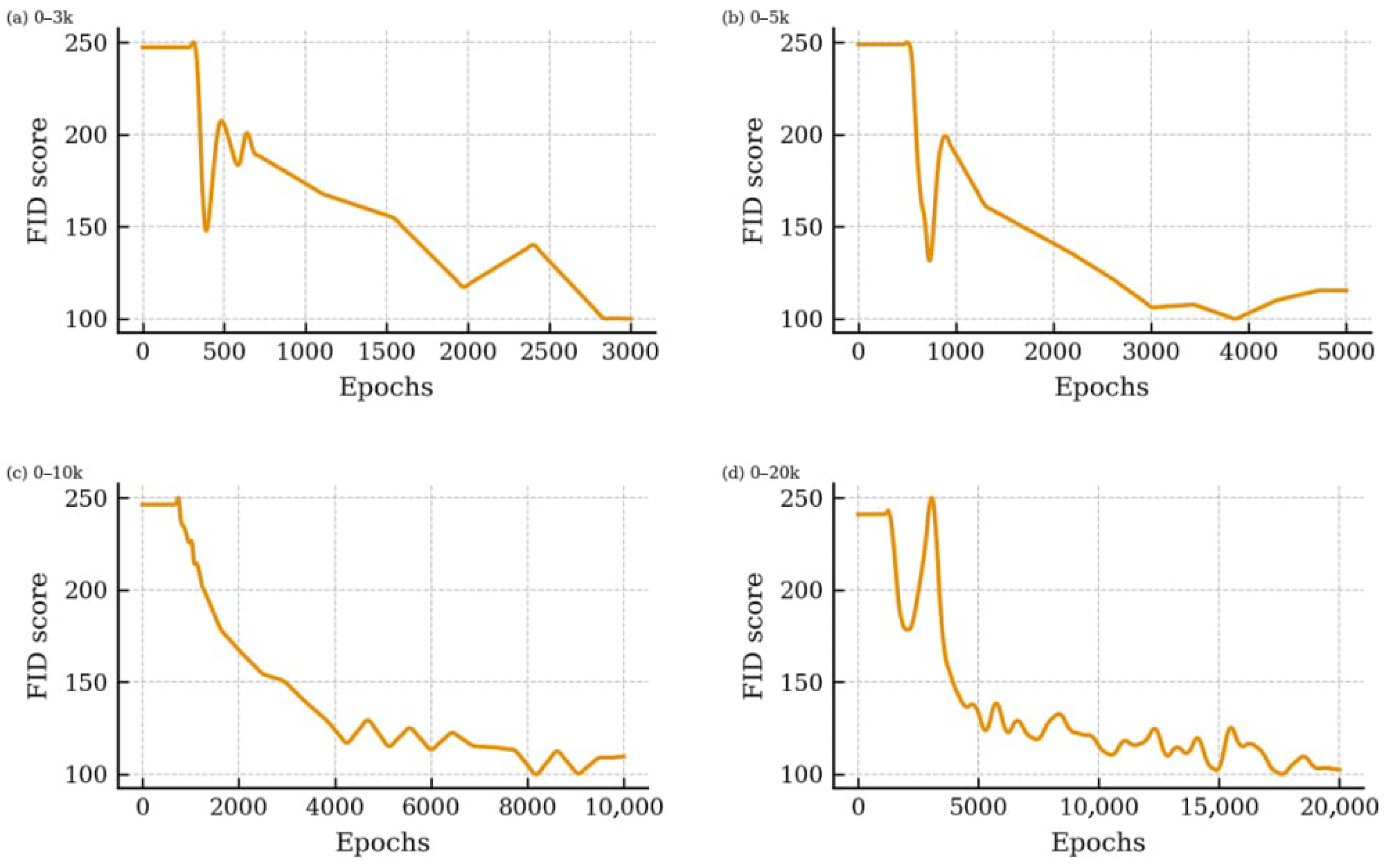
Figure A2.
Convergence of FID score for DCGAN trained on the wind dataset.
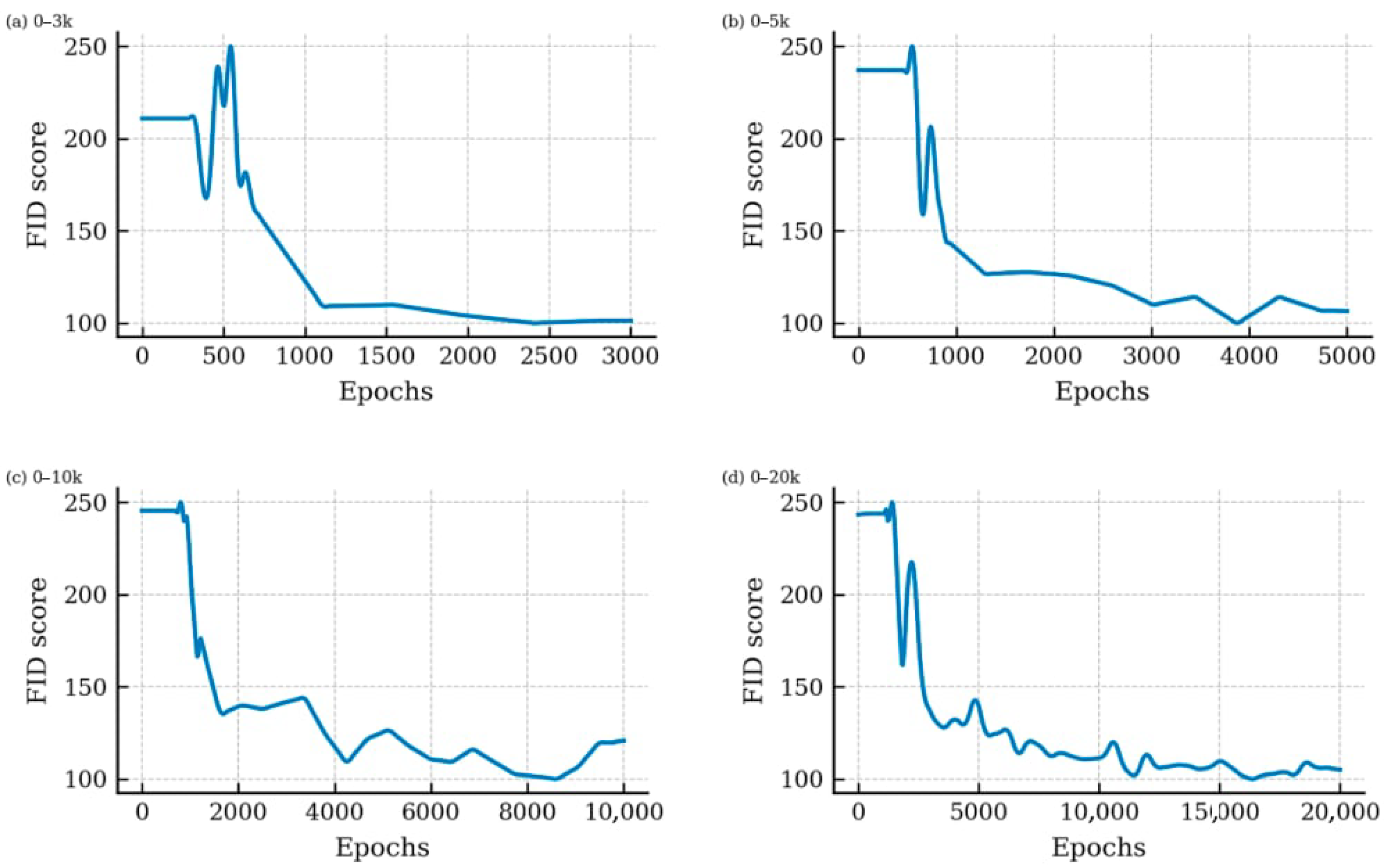
Figure A3.
Representative daily PV power output curves under five clustered operating states.
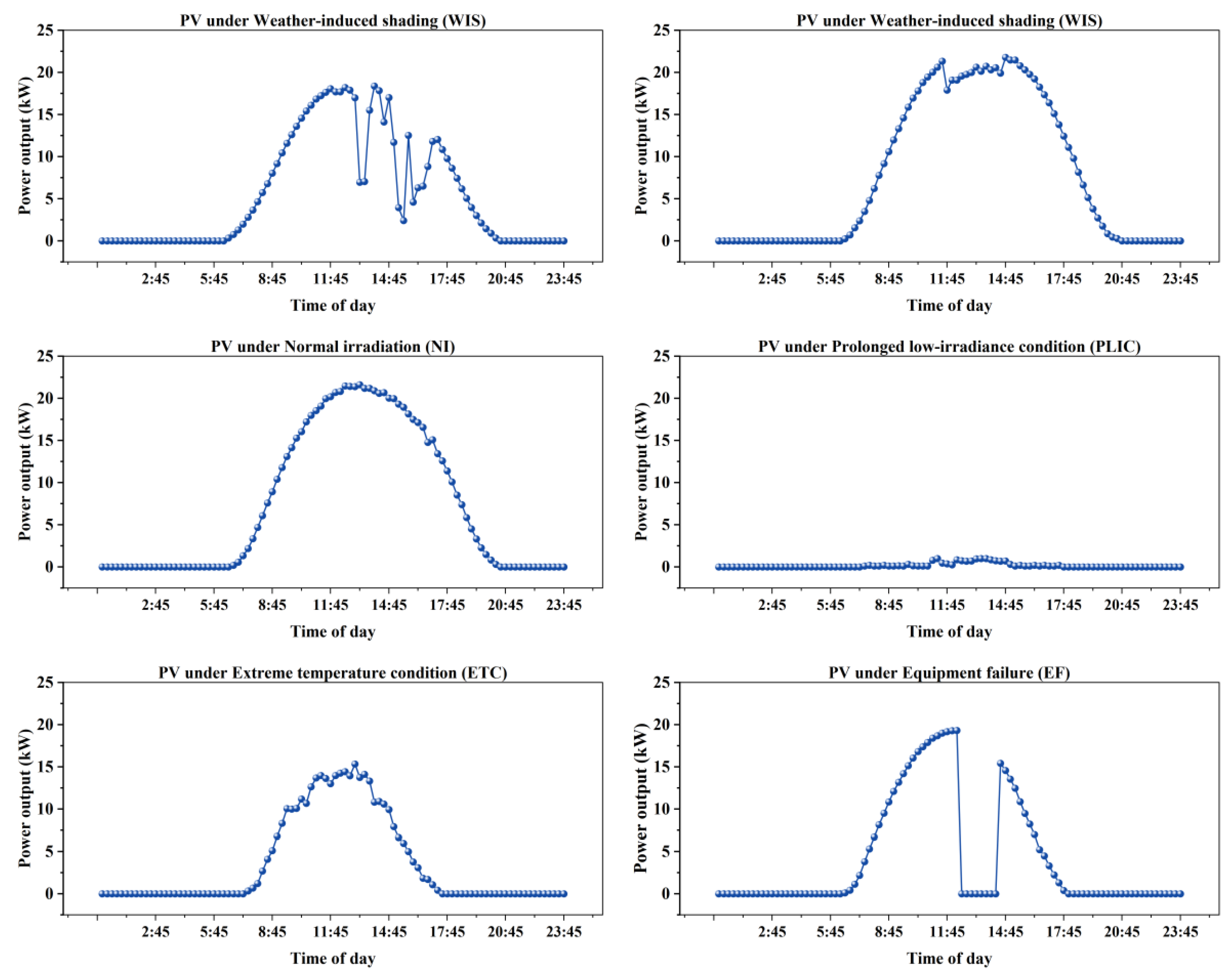
Figure A4.
Representative daily wind power output curves under five clustered operating states.
Appendix B. 2D-CNN Training-Validation Curves on Imbalanced Wind/PV–Wind Datasets
Figure A5.
Training and validation curves (accuracy/loss) for the deep-learning model trained on imbalanced wind power data.
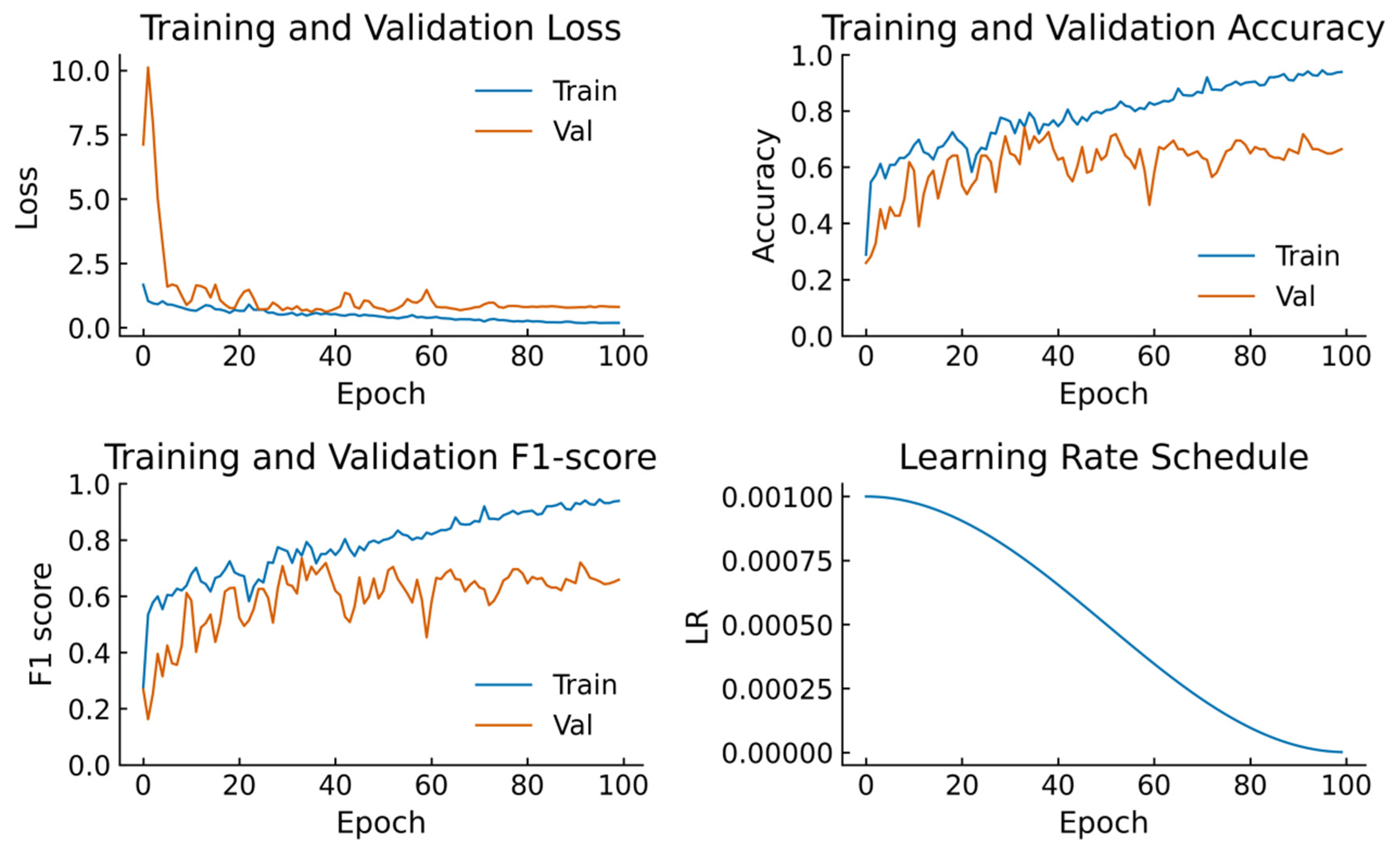
Figure A6.
Training and validation curves (accuracy/loss) for the deep-learning model trained on an imbalanced hybrid PV and wind power dataset.
References
- International Energy Agency (IEA). Renewables 2025: Analysis and Forecast to 2030; IEA: Paris, France, 2025. [Google Scholar]
- International Energy Agency (IEA). Renewables 2020: Analysis and Forecast to 2025; IEA: Paris, France, 2020. [Google Scholar]
- Zhang, X.; Li, Z. A survey on photovoltaic array fault diagnosis algorithms. Intell. Comput. Appl. 2022, 12, 143–147. (In Chinese) [Google Scholar]
- Huang, L.L.; Fu, Y.; Ren, H.H.; Wei, S.R.; Huang, Y.S. Review of Wind Turbine Maintenance Based on Condition Monitoring Systems. Proc. CSEE 2020, 40, 7065–7077. [Google Scholar] [CrossRef]
- Wang, H.; Li, T.; Xie, M.; Tian, W.; Han, W. Wind Turbine Fault Diagnosis with Imbalanced SCADA Data Using Generative Adversarial Networks. Energies 2025, 18, 1158. [Google Scholar] [CrossRef] [Scilit]
- Oliveira-Filho, A.; Comeau, M.; Cave, J.; Nasr, C.; Côté, P.; Tahan, A. Wind Turbine SCADA Data Imbalance: A Review of Its Impact on Health Condition Analyses and Mitigation Strategies. Energies 2025, 18, 59. [Google Scholar] [CrossRef] [Scilit]
- Sonawane, P.R.; Bhandari, S.; Patil, R.B.P.; Al-Dahidi, S. Comparative analysis of methods used to solve class imbalance problem in dataset for CNN-based fault diagnosis of solar photovoltaic panels. Int. J. Thermofluids 2025, 28, 101303. [Google Scholar] [CrossRef] [Scilit]
- Wang, Z.; Cui, Q.; Gong, Z.; Shi, L.; Gao, J.; Zhong, J. Anomaly Identification for Photovoltaic Power Stations Using a Dual Classification System and Gramian Angular Field Visualization. Processes 2024, 12, 690. [Google Scholar] [CrossRef] [Scilit]
- Wang, Z.; Oates, T. Encoding Time Series as Images for Visual Inspection and Classification Using Tiled Convolutional Neural Networks. In Trajectory-Based Behavior Analytics: Papers from the 2015 AAAI Workshop (AAAIW-15); AAAI Press: Menlo Park, CA, USA, 2015; pp. 40–46. [Google Scholar]
- Rangel-Rodriguez, A.H.; Amezquita-Sanchez, J.P.; Granados-Lieberman, D.; Camarena-Martinez, D.; Bueno-Lopez, M.; Valtierra-Rodriguez, M. A Gramian Angular Field-Based Convolutional Neural Network Approach for Crack Detection in Low-Power Turbines from Vibration Signals. Information 2025, 16, 775. [Google Scholar] [CrossRef] [Scilit]
- Iwana, B.K.; Uchida, S. An empirical survey of data augmentation for time series classification with neural networks. PLoS ONE 2021, 16, e0254841. [Google Scholar] [CrossRef] [Scilit] [PubMed]
- Mou, J.; Liu, W.; Xiong, W. Industrial process fault detection based on bidirectional generative adversarial networks. CAAI Trans. Intell. Syst. 2024, 19, 1199–1208. (In Chinese) [Google Scholar] [CrossRef]
- Sylolypavan, A.; Sleeman, D.; Wu, H.; Sim, M. The impact of inconsistent human annotations on AI driven clinical decision making. npj Digit Med. 2023, 6, 26. [Google Scholar] [CrossRef] [Scilit] [PubMed]
- Maldonado-Correa, J.; Martín-Martínez, S.; Artigao, E.; Gómez-Lázaro, E. Using SCADA data for wind turbine condition monitoring: A systematic literature review. Energies 2020, 13, 3132. [Google Scholar] [CrossRef] [Scilit]
- Shen, J.; Wu, Z.; Cao, Y.; Zhang, Q.; Cui, Y. Research on fault diagnosis of rolling bearing based on Gramian angular field and lightweight model. Sensors 2024, 24, 5952. [Google Scholar] [CrossRef] [Scilit] [PubMed]
- Zhou, Y.; Long, X.; Sun, M.; Chen, Z. Bearing fault diagnosis based on Gramian angular field and DenseNet. Math. Biosci. Eng. 2022, 19, 14086–14101. [Google Scholar] [CrossRef] [Scilit] [PubMed]
- Xu, C.; Xu, C.; Xu, Y.; Zhang, L.; Hu, Z.; Song, H. Fault diagnosis method of wind turbine planetary gearbox based on Gramian angular difference fields and deep learning. Sci. Rep. 2025, 15, 14243. [Google Scholar] [CrossRef] [Scilit] [PubMed]
- Liu, X.; Lu, S.; Ren, Y.; Wu, Z. Wind turbine anomaly detection based on SCADA data mining. Electronics 2020, 9, 751. [Google Scholar] [CrossRef] [Scilit]
- Song, X.; Liu, Y. Wind and Photovoltaic Generation Scene Division Based on Improved K-means Clustering. Power Gener. Technol. 2020, 41, 625–630. (In Chinese) [Google Scholar] [CrossRef]
- Cheung, W.Y.; Thomson, L. Using K-Means-derived pseudo-labels and machine learning classification on Sentinel-2 imagery to delineate snow cover ratio and snowline altitude. Remote Sens. 2025, 17, 3872. [Google Scholar] [CrossRef] [Scilit]
- Chen, H.; Wei, J.; Huang, H.; Yuan, Y.; Wang, J. Review of imbalanced fault diagnosis technology based on generative adversarial networks. J. Comput. Des. Eng. 2024, 11, 99–124. [Google Scholar] [CrossRef] [Scilit]
- Zhao, J.; Fang, Q.; Chang, Y.; Zhang, Y.; Tao, T. Data augmentation method based on DCGAN for class imbalance in mechanical fault diagnosis. Sci. Rep. 2025, 15, 14115. [Google Scholar] [CrossRef] [Scilit] [PubMed]
- Sokolova, M.; Lapalme, G. A systematic analysis of performance measures for classification tasks. Inf. Process. Manag. 2009, 45, 427–437. [Google Scholar] [CrossRef] [Scilit]
- Maldonado, S.; Vairetti, C.; Jara, K.; Carrasco, M.; López, J. OWAdapt: An adaptive loss function for deep learning using OWA operators. Knowl.-Based Syst. 2023, 280, 111022. [Google Scholar]
- Imani, M. Imbalanced data classification using graph based transformation. Sci. Rep. 2025, 15, 33415. [Google Scholar] [CrossRef] [Scilit] [PubMed]
- Kumar, V.; Lalotra, G.S.; Sasikala, P.; Rajput, D.S.; Kaluri, R.; Lakshmanna, K.; Shorfuzzaman, M.; Alsufyani, A.; Uddin, M. Addressing Binary Classification over Class Imbalanced Clinical Datasets Using Computationally Intelligent Techniques. Healthcare 2022, 10, 1293. [Google Scholar] [CrossRef] [Scilit] [PubMed]
- Chen, G.; Hou, B. Oversampling Algorithms for Gaussian-type Data Based on Generative Adversarial Networks. Inf. Control 2024, 53, 182–190. (In Chinese) [Google Scholar] [CrossRef]
- Wang, X.; Liu, B.; Sun, K.; Zhao, J.; Chen, L. A Review of Photovoltaic Array Fault Diagnosis Technology. Trans. China Electrotech. Soc. 2024, 39, 6526–6543. (In Chinese) [Google Scholar] [CrossRef]
- Kumari, N.; Singh, S.K.; Kumar, S.; Jadoun, V.K. Performance analysis of partially shaded high-efficiency mono PERC/mono crystalline PV module under indoor and environmental conditions. Sci. Rep. 2024, 14, 21587. [Google Scholar] [CrossRef] [Scilit] [PubMed]
- Huang, B.; Zhou, Z.J.; Li, Z.N.; Gong, B.; Wang, X.J.; Dong, J.S.; Liu, X.J. Research progress on the impact of wind-sand flow on desert photovoltaic modules and their power generation efficiency. Acta Aerodyn. Sin. 2025, 43, 64–79. [Google Scholar] [CrossRef]
- Williams, R.A.; Lizzadro-McPherson, D.J.; Pearce, J.M. The impact of snow losses on solar photovoltaic systems in North America in the future. Energy Adv. 2023, 2, 1634–1649. [Google Scholar] [CrossRef] [Scilit]
- Shaik, F.; Lingala, S.S.; Veeraboina, P. Effect of various parameters on the performance of solar PV power plant: A review and the experimental study. Sustain. Energy Res. 2023, 10, 6, Correction in Sustain. Energy Res. 2025, 12, 33. [Google Scholar] [CrossRef] [Scilit]
- Chen, H.; Xie, C.; Dai, J.; Cen, E.; Li, J. SCADA Data-Based Working Condition Classification for Condition Assessment of Wind Turbine Main Transmission System. Energies 2021, 14, 7043. [Google Scholar] [CrossRef] [Scilit]
- Ma, Y.; Liu, Y.; Yang, Z.; Yan, J.; Tao, T.; Infield, D. Research on the Derated Power Data Identification Method of a Wind Turbine Based on a Multi-Gaussian–Discrete Joint Probability Model. Sensors 2022, 22, 8891. [Google Scholar] [CrossRef] [Scilit] [PubMed]
- Gao, D.W.; Muljadi, E.; Tian, T.; Miller, M. Comparison of Standards and Technical Requirements of Grid-Connected Wind Power Plants in China and the United States; NREL Technical Report NREL/TP-5D00-64225; NREL: Golden, CO, USA, 2016. [Google Scholar]
- Anderson, B.; Baring-Gould, E. Demonstration of a Fault Impact Reduction Control Module for Wind Turbines. Wind Energ. Sci. 2022, 7, 1753–1769. [Google Scholar] [CrossRef] [Scilit]
- Velandia-Cardenas, C.; Vidal, Y.; Pozo, F. Wind Turbine Fault Detection Using Highly Imbalanced Real SCADA Data. Energies 2021, 14, 1728. [Google Scholar] [CrossRef] [Scilit]
- Mei, X.; Yang, Y. Effects of Seismic Load on Dynamic Response of a 15 MW Offshore Wind Turbine. J. Chin. Soc. Power Eng. 2022, 42, 150–155. (In Chinese) [Google Scholar] [CrossRef]
- Zhao, S.; Gui, J.; Dong, M.; Yu, B.; Gui, Z.; Dong, L.; Tang, Y.Y.; Kwok, J.T.-Y. A Survey on Small Sample Imbalance Problem: Metrics, Feature Analysis, and Solutions. arXiv 2025, arXiv:2504.14800. [Google Scholar] [CrossRef] [Scilit]
- Liu, X.Y.; Wu, J.; Zhou, Z.H. Learning Imbalanced Multi-class Data with Optimal Dichotomy Weights. In Proceedings of the 2013 IEEE 13th International Conference on Data Mining (ICDM 2013); IEEE: Piscataway, NJ, USA, 2013; pp. 478–487. [Google Scholar] [CrossRef] [Scilit]
- Wang, S.; Yao, X. Multiclass imbalance problems: Analysis and potential solutions. IEEE Trans. Syst. Man Cybern. B Cybern. 2012, 42, 1119–1130. [Google Scholar] [CrossRef] [Scilit] [PubMed]
- Tang, W.H.; Niu, Z.W.; Zhao, B.N.; Ji, T.Y.; Li, M.S.; Wu, Q.H. Research and application of data-driven artificial intelligence technology for condition analysis of power equipment. High Volt. Eng. 2020, 46, 2985–2999. [Google Scholar] [CrossRef]
- Venu, S.K.; Ravula, S. Evaluation of Deep Convolutional Generative Adversarial Networks for Data Augmentation of Chest X-ray Images. Future Internet 2021, 13, 8. [Google Scholar] [CrossRef] [Scilit]
- Gulrajani, I.; Ahmed, F.; Arjovsky, M.; Dumoulin, V.; Courville, A. Improved Training of Wasserstein GANs. Adv. Neural Inf. Process. Syst. 2017, 30, 5767–5777. [Google Scholar] [CrossRef] [Scilit]
- Radford, A.; Metz, L.; Chintala, S. Unsupervised Representation Learning with Deep Convolutional Generative Adversarial Networks. arXiv 2015, arXiv:1511.06434. [Google Scholar]
- Loshchilov, I.; Hutter, F. SGDR: Stochastic Gradient Descent with Warm Restarts. arXiv 2016, arXiv:1608.03983. [Google Scholar] [CrossRef] [Scilit]
- Heusel, M.; Ramsauer, H.; Unterthiner, T.; Nessler, B.; Hochreiter, S. GANs Trained by a Two Time-Scale Update Rule Converge to a Local Nash Equilibrium. Adv. Neural Inf. Process. Syst. 2017, 30, 6626–6637. [Google Scholar] [CrossRef] [Scilit]
- Aleixandre-Tudó, J.L.; Castelló-Cogollos, L.; Aleixandre-Benavent, R. Renewable energies: Worldwide trends in research, funding and international collaboration. Renew. Energy 2019, 139, 268–278. [Google Scholar] [CrossRef] [Scilit]
- Zhou, J.; Lu, X.; Xiao, Y.; Tang, J.; Su, J.; Li, Y.; Liu, J.; Lyu, J.; Ma, Y.; Dou, D. A Dataset for Spatial Dynamic Wind Power Forecasting over a Large Turbine Array. Sci. Data 2024, 11, 649. [Google Scholar]
- Wang, Z.; Oates, T. Imaging Time-Series to Improve Classification and Imputation. In The Twenty-Fourth International Joint Conference on Artificial Intelligence; 2015; pp. 3939–3944. Available online: https://ijcai.org/proceedings/2015/553 (accessed on 13 November 2026).
- Wang, D.; Sun, Z. A method for cluster analysis of electric power consumers based on in-memory computing. CAAI Trans. Intell. Syst. 2015, 10, 569–576. [Google Scholar] [CrossRef]
- Hartigan, J.A.; Wong, M.A. Algorithm AS 136: A K-Means Clustering Algorithm. Appl. Stat. 1979, 28, 100–108. [Google Scholar] [CrossRef] [Scilit]
- van der Maaten, L.; Hinton, G. Visualizing Data using t-SNE. J. Mach. Learn. Res. 2008, 9, 2579–2605. Available online: https://www.jmlr.org/papers/v9/vandermaaten08a.html (accessed on 13 November 2026).
- Hou, Q.; Du, E.; Tian, X.; Liu, F.; Zhang, N.; Kang, C. Data-driven Power System Operation Mode Analysis. Proc. CSEE 2021, 41, 1–12. [Google Scholar] [CrossRef]
- Chu, Y.Z.; Shi, Y.J.; Zhang, X.F.; Liu, H. Image classification algorithm based on split channel attention network. Chin. J. Eng. 2024, 46, 1856–1863. (In Chinese) [Google Scholar] [CrossRef]
- Srivastava, N.; Hinton, G.; Krizhevsky, A.; Krizhevsky, A.; Sutskever, I.; Salakhutdinov, R. Dropout: A Simple Way to Prevent Neural Networks from Overfitting. J. Mach. Learn. Res. 2014, 15, 1929–1958. Available online: https://www.jmlr.org/papers/v15/srivastava14a.html (accessed on 13 November 2026).
- Loshchilov, I.; Hutter, F. Decoupled Weight Decay Regularization. arXiv 2019, arXiv:1711.05101. [Google Scholar] [CrossRef] [Scilit]
- Micikevicius, P.; Narang, S.; Alben, J.; Diamos, G.; Elsen, E.; Garcia, D.; Ginsburg, B.; Houston, M.; Kuchaev, O.; Venkatesh, G.; et al. Mixed Precision Training. arXiv 2018, arXiv:1710.03740. [Google Scholar] [CrossRef] [Scilit]
- Powers, D.M.W. Evaluation: From precision, recall and F-measure to ROC, informedness, markedness & correlation. J. Mach. Learn. Technol. 2011, 2, 37–63. [Google Scholar] [CrossRef] [Scilit]
- Saito, T.; Rehmsmeier, M. The Precision-Recall Plot Is More Informative than the ROC Plot When Evaluating Binary Classifiers on Imbalanced Datasets. PLoS ONE 2015, 10, e0118432. [Google Scholar] [CrossRef] [Scilit] [PubMed]
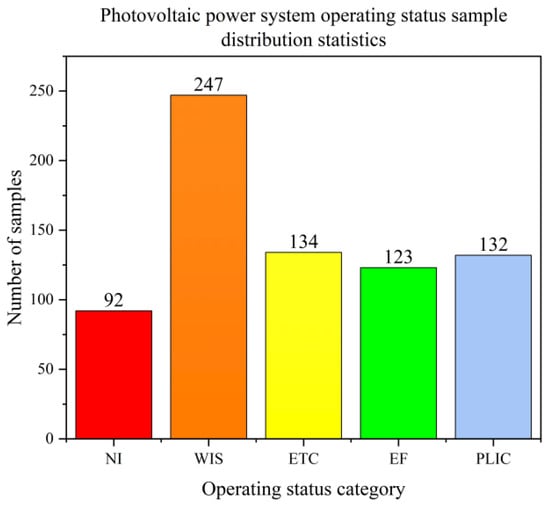
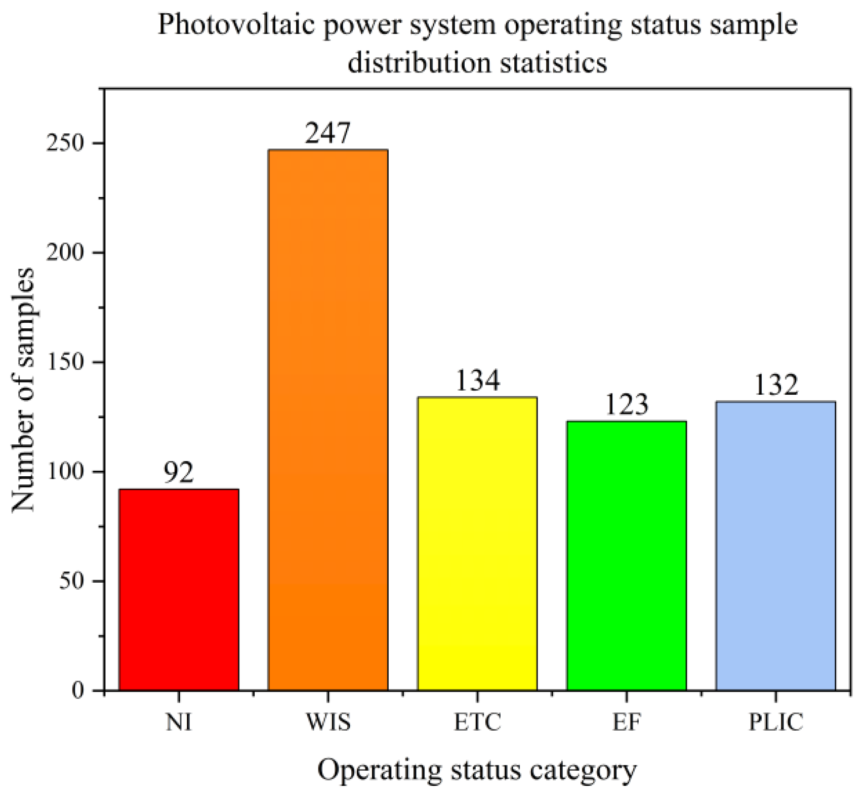
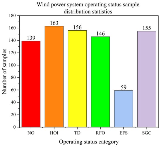
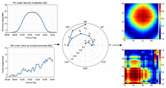
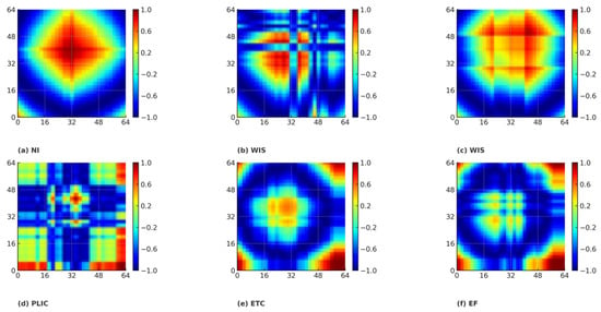
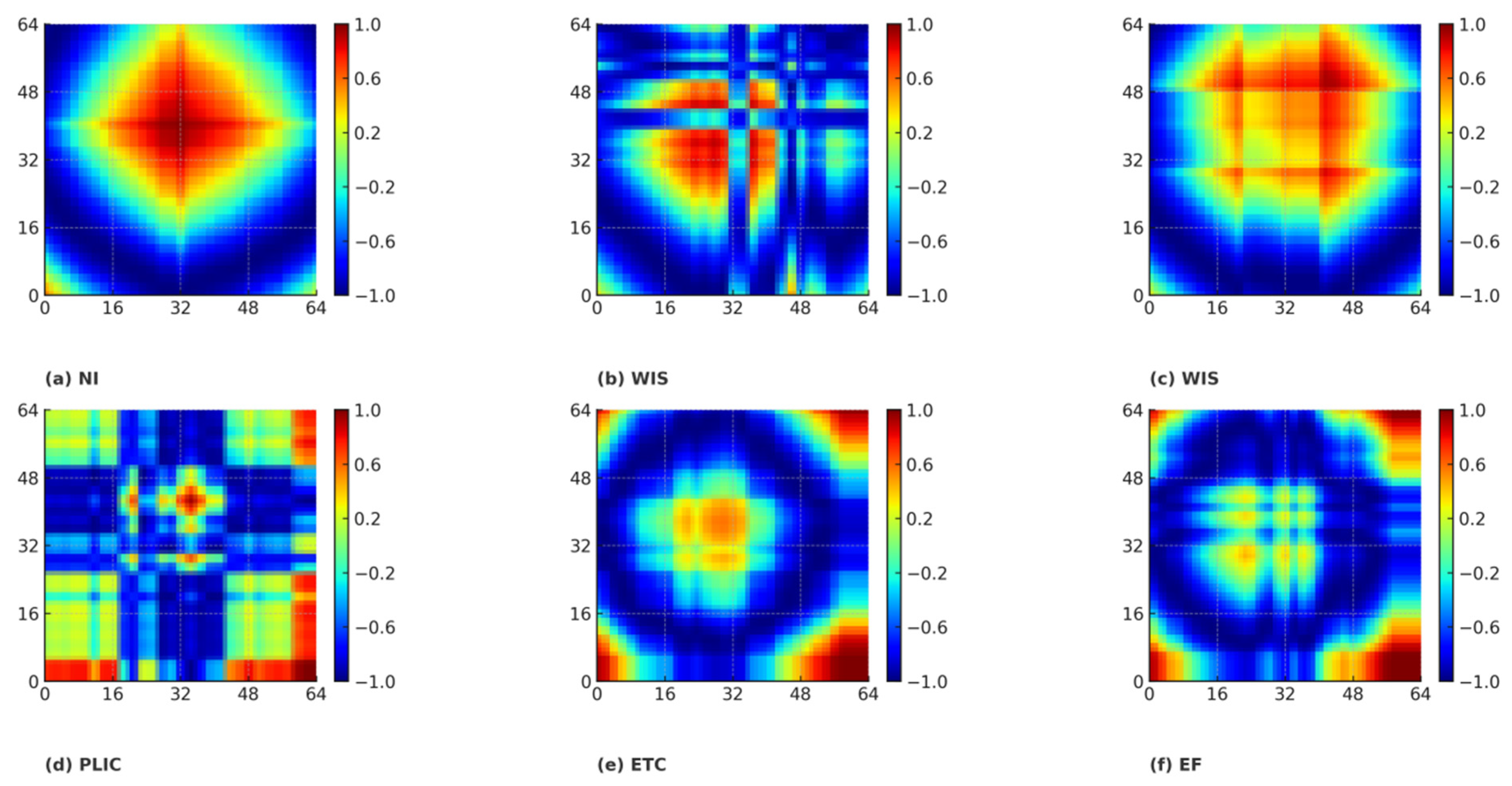
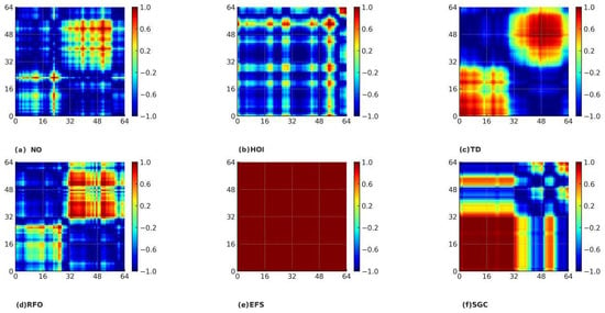
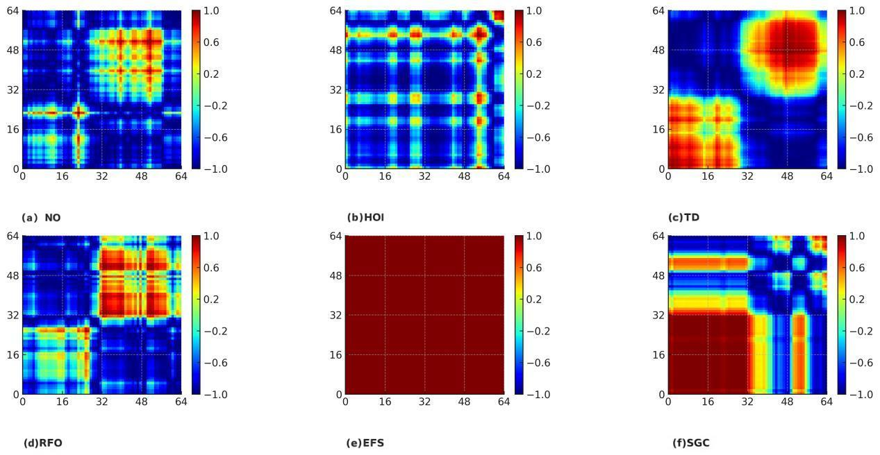
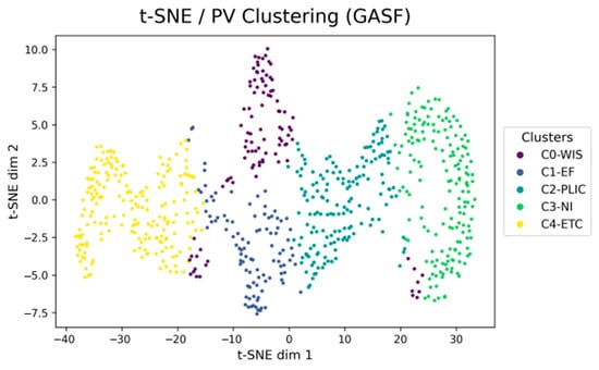
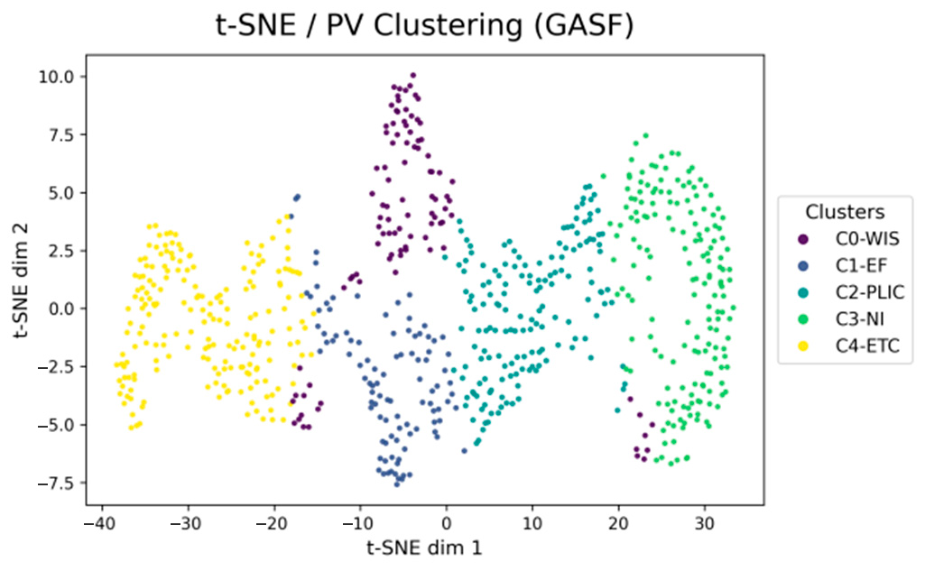
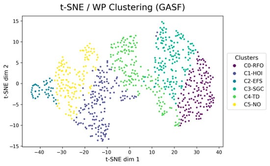
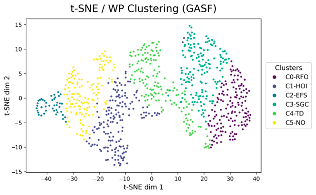
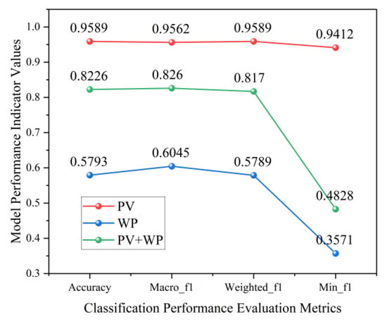
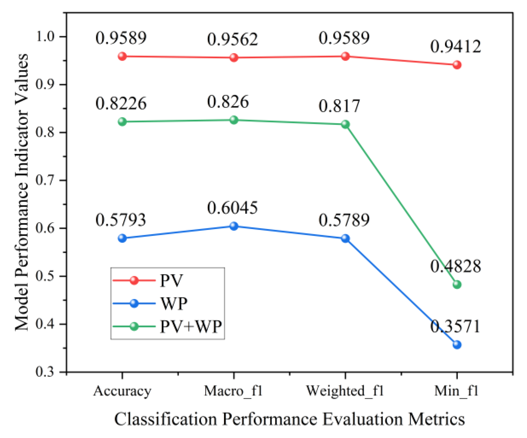
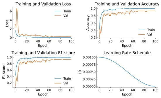
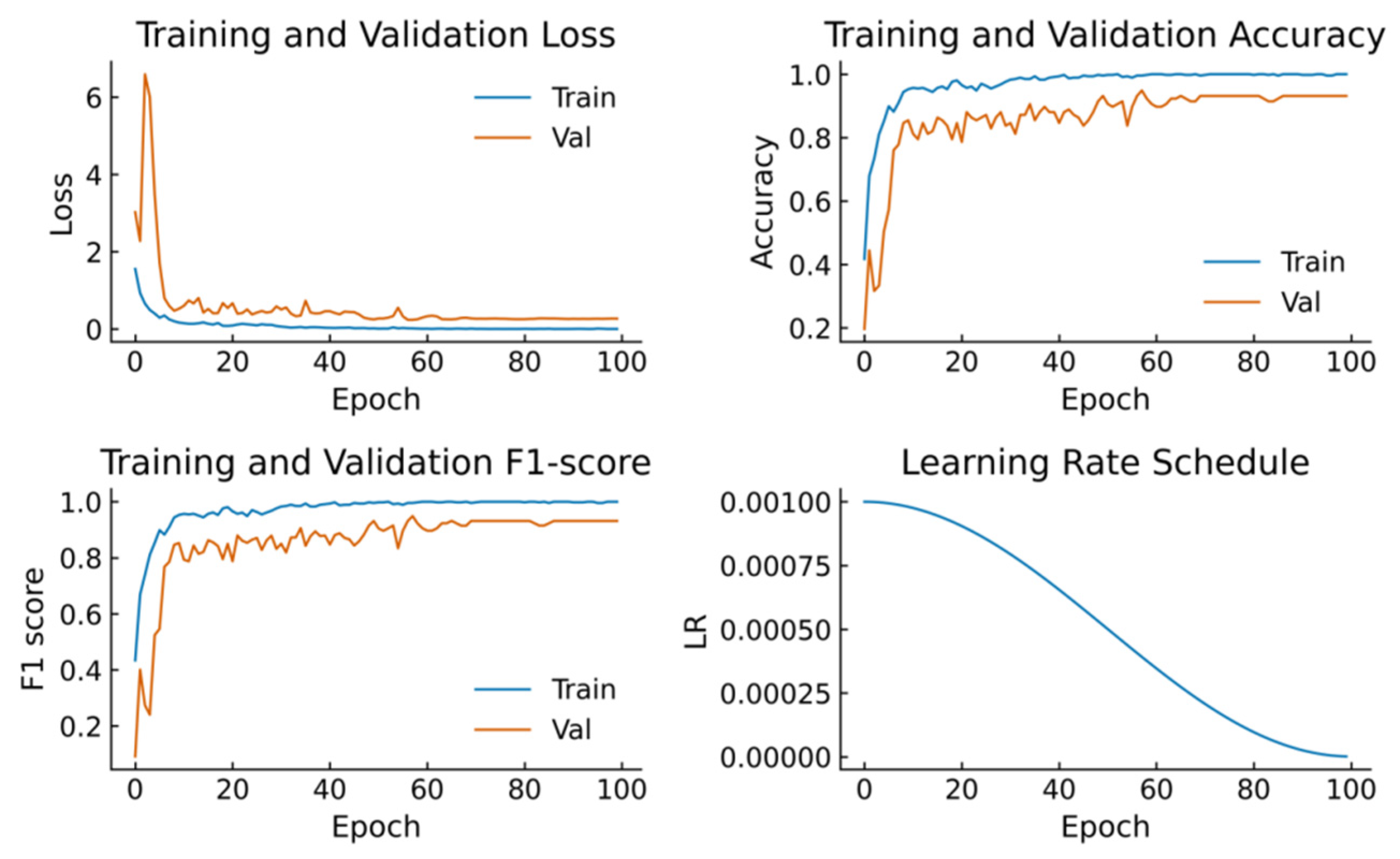
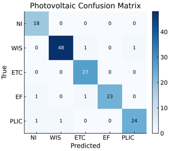
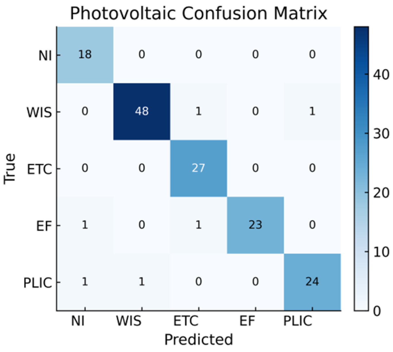
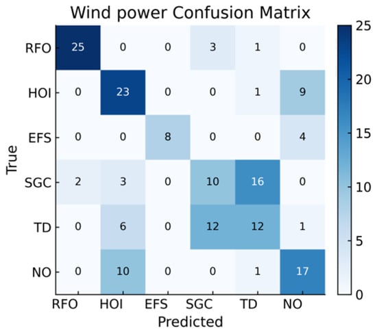
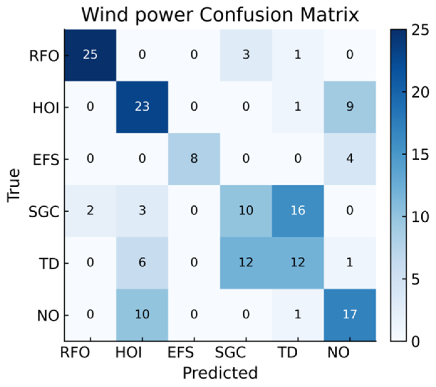
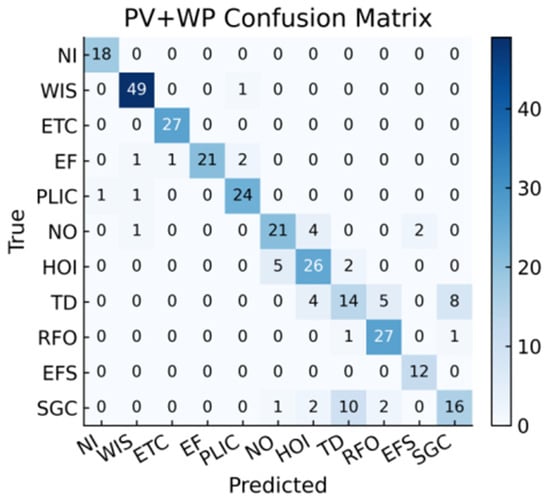
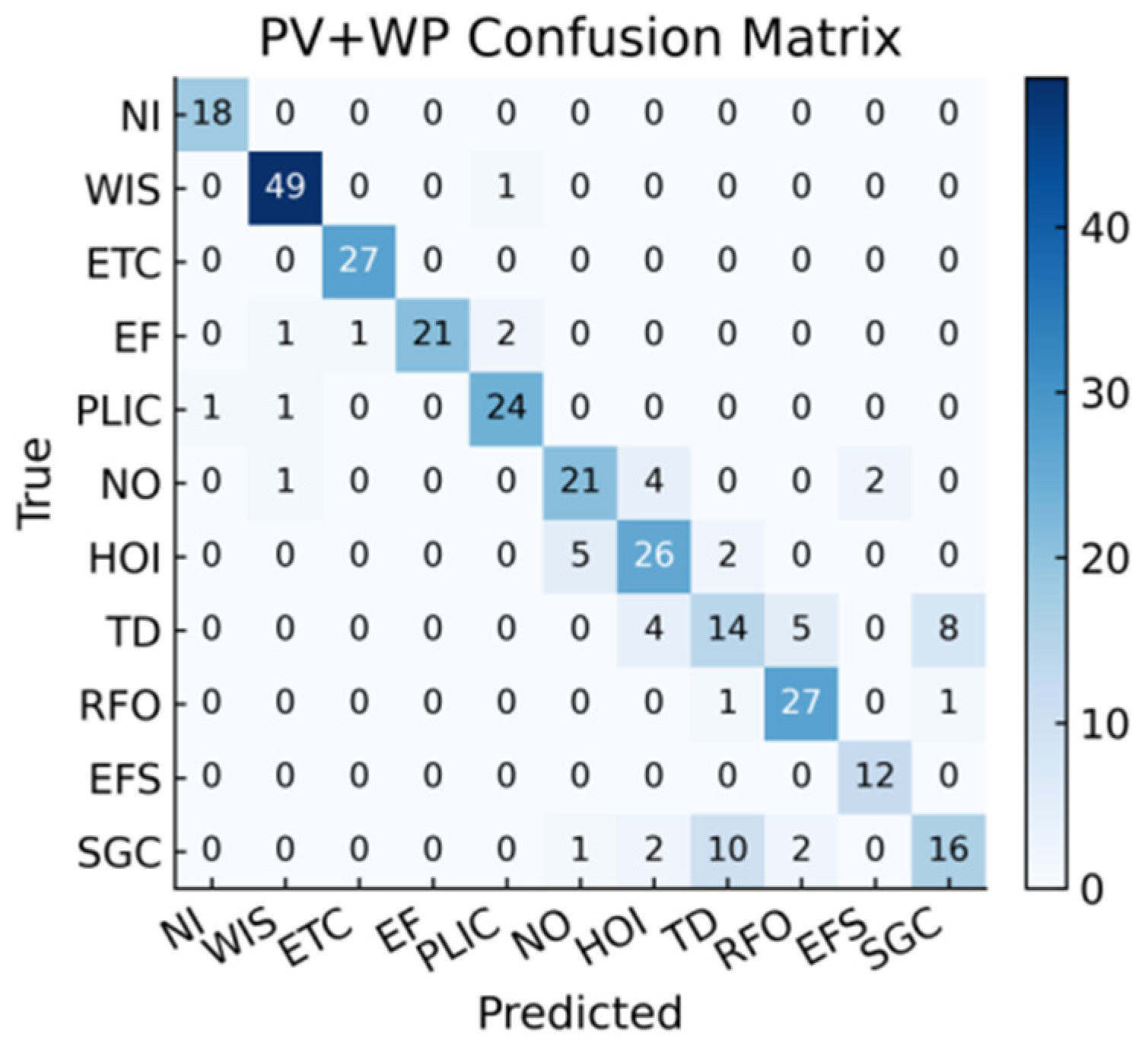
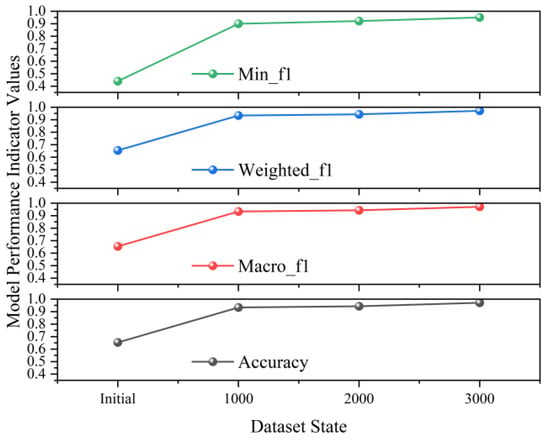
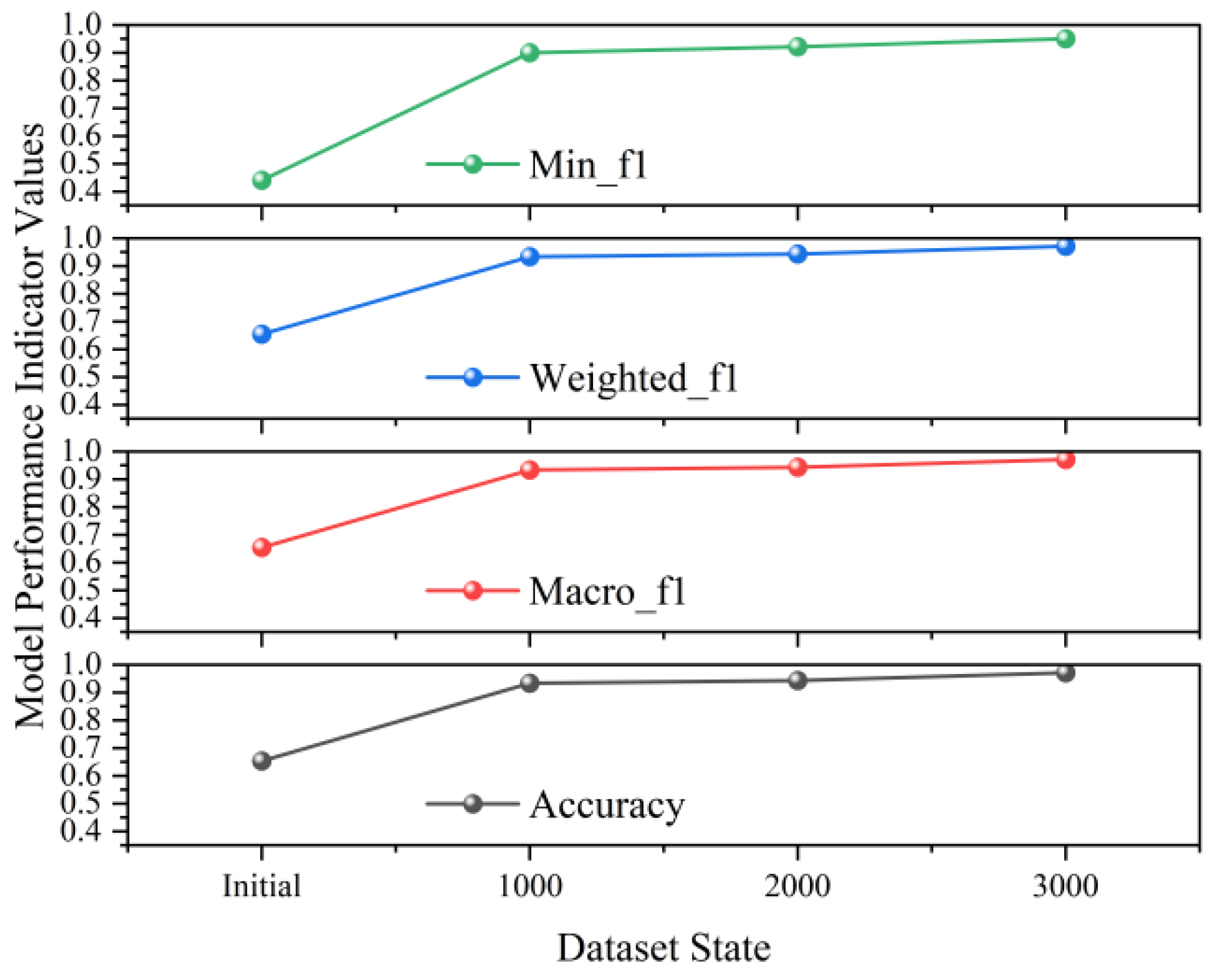
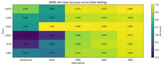
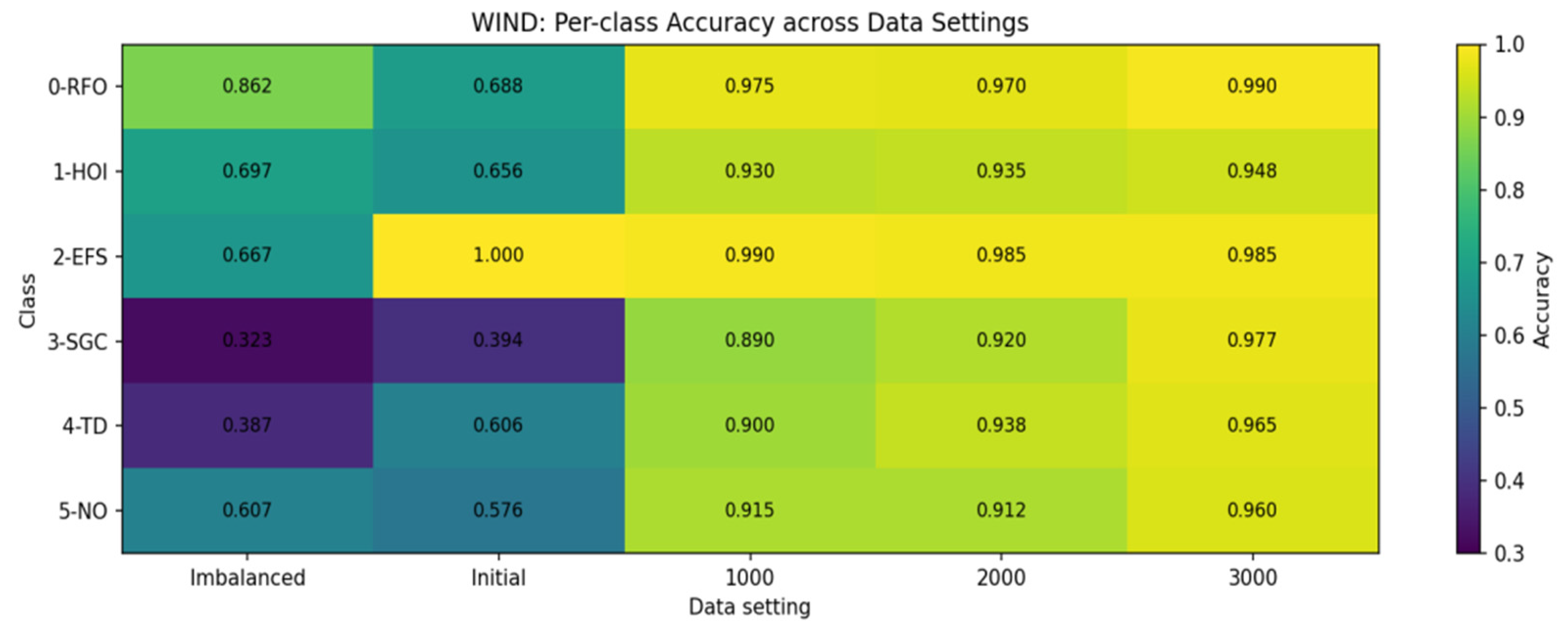
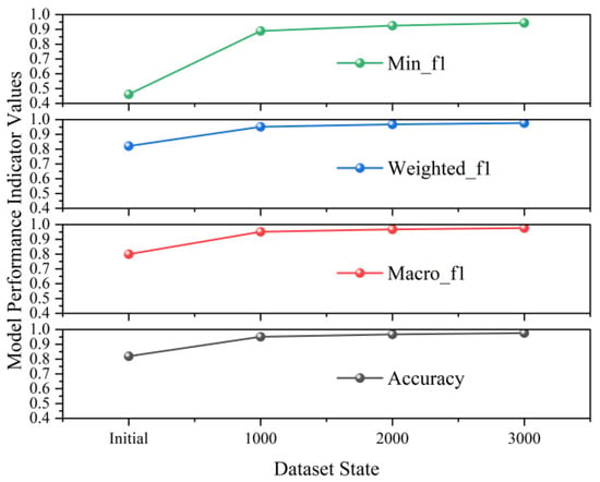
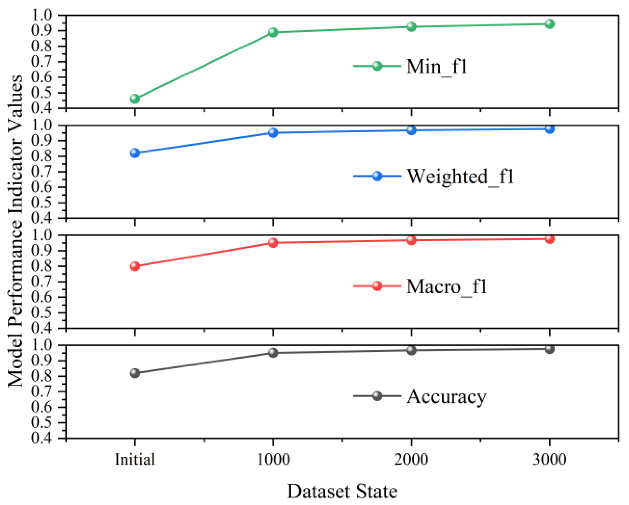
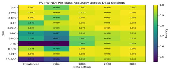
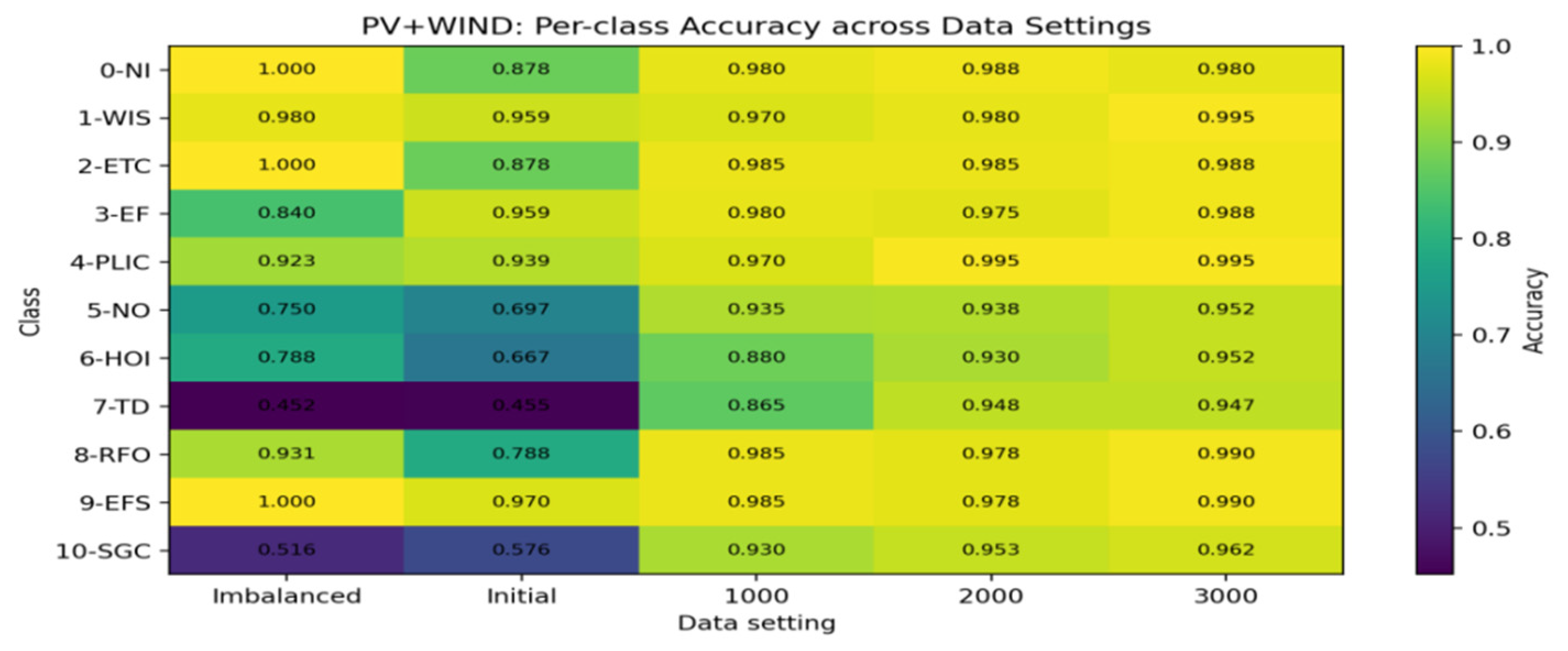
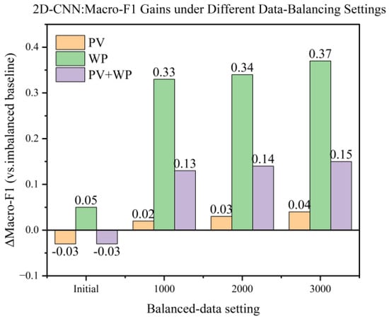
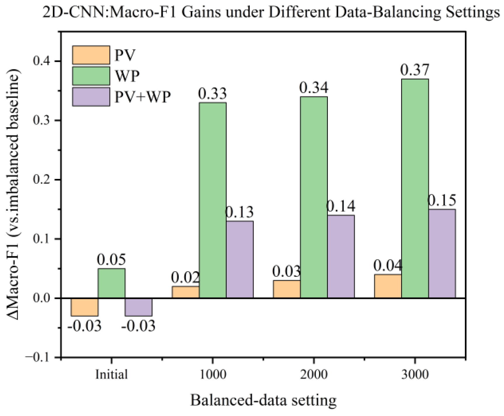
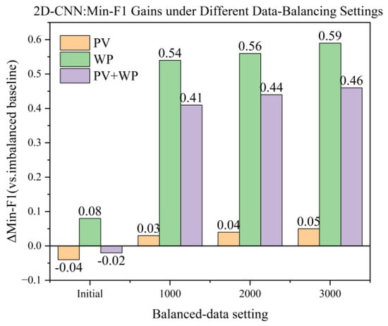
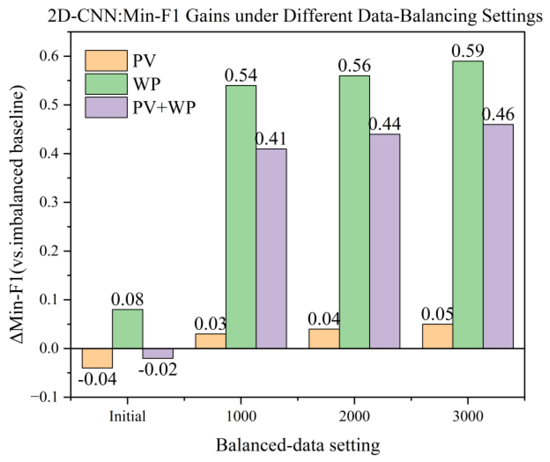

Disclaimer/Publisher’s Note: The statements, opinions and data contained in all publications are solely those of the individual author(s) and contributor(s) and not of MDPI and/or the editor(s). MDPI and/or the editor(s) disclaim responsibility for any injury to people or property resulting from any ideas, methods, instructions or products referred to in the content. |
© 2026 by the authors. Licensee MDPI, Basel, Switzerland. This article is an open access article distributed under the terms and conditions of the Creative Commons Attribution (CC BY) license.