Heat Transfer Enhancement and Latent Thermal Energy Storage in Greenhouses Using Phase Change Material–Metal Foam Composites: A CFD Investigation

Abstract

Greenhouses operating in hot, arid climates are exposed to large solar gains during the day and significant heat losses at night, which makes passive thermal buffering attractive. In this work, a north-wall storage layer made of the paraffin RT25 is embedded in aluminum, copper or steel foam, and its effect on the greenhouse microclimate is analyzed with a transient two-dimensional CFD model that couples porous-medium resistance, discrete-ordinates solar radiation, turbulent airflow and enthalpy–porosity phase change. Each composite is evaluated against an otherwise identical pure-RT25 wall. The simulated temperature, liquid-fraction, enthalpy and velocity fields show that the foam material modifies conductive heat spreading inside the wall, the timing of latent storage and the buoyancy-driven circulation in the enclosure. The thermal and phase-change results correspond to a 45 °C exterior/15 °C nighttime scenario, while the airflow profiles correspond to a separate 45 °C/10 °C scenario. A single foam pore density (20 PPI) is examined, so no pore-density optimum is claimed. Against a building-roof PCM experiment, the model reproduces the measured inner roof-surface temperature history with a root-mean-square error of 0.21 °C; this benchmark supports the thermal response of the PCM layer but not the complete greenhouse–foam system. Because no HVAC load balance is solved, the findings are expressed as comparative physical responses rather than as quantified energy savings.

1. Introduction

Rising world population and growing pressure on water, land and energy resources make it necessary to produce food at a lower cost and with less energy. Greenhouses address part of this challenge by providing a controlled growing environment in which the microclimate can be adapted to the crop, allowing cultivation throughout the year and higher yields per unit area [1,2,3,4,5]. Large greenhouse complexes have proved successful in the temperate climates of Europe; in tropical and subtropical regions, however, high summer temperatures and humidity create specific design problems, and some form of cooling is usually required to avoid overheating [1,6,7]. Natural ventilation is the simplest cooling option, but its effectiveness depends on the greenhouse type, the state of the crop, the outdoor weather and several other factors [8], so the indoor and outdoor environmental conditions must be characterized before ventilation can be controlled effectively. Using transient two-dimensional CFD simulations, Villagrán et al. [9] analyzed the temperature field of three naturally ventilated greenhouse types; after validating their model, they showed that natural ventilation reduced the high summer air temperatures in all three structures.

Thermal storage in the building envelope is a second passive strategy. Berroug et al. [10] modeled a solar greenhouse whose north wall contained a PCM, describing heat transfer in the PCM layer one-dimensionally; under their conditions, a 4 cm PCM plate raised both the air temperature near the crop and the mean air temperature by roughly 6.0–12.0 °C. Zhang et al. [11] proposed a three-layer straw-block north wall (240 mm storage, 100 mm insulation and 160 mm heat-preservation layers) and reported indoor maximum temperatures 2.0 °C and 2.1 °C higher than those of a porous clay-block wall on overcast and sunny days, respectively, with smaller indoor temperature swings owing to the higher storage capacity of the straw wall. In the building sector, Diarce et al. [12,13] studied a ventilated active façade containing PCM and found that it captured about 10–12% of the incident solar radiation and increased the mean indoor temperature by 1.1 °C. Mirahmad and Sadrameli [14] developed a one-dimensional model of a PCM-equipped greenhouse and concluded that the heat-capacity method is better suited when the PCM melts over a wide temperature range. Guan et al. [15] built a three-dimensional CFD model of a latent-heat ventilated wall and examined how the ventilation air speed affects heat storage and release, the largest release being obtained at 4 m/s. Active solutions have also been tested: a burning-cave hot-water soil heating system raised the mean soil temperature of an experimental greenhouse by 5–6 °C [16], and a stand-alone system combining photovoltaic, hydrogen and geothermal technologies was proposed for winter heating [17]. Such active equipment, however, tends to be expensive, bulky and demanding to maintain. Surface engineering of heat-exchange components has been explored as well: Ganesan et al. [18] reviewed the air-side performance of heat exchangers with hydrophilic, hydrophobic and uncoated fins, noting that hydrophilic fins drain condensate and therefore suffer smaller performance losses, while Wang et al. [19] showed that hybrid superhydrophilic–superhydrophobic copper surfaces (600 × 600 μm² patches with 600 μm spacing) achieved heat-transfer coefficients 1.1 and 1.3 times those of the two uniform surfaces and heat fluxes 31–73% higher than a fully superhydrophobic surface, owing to faster droplet nucleation combined with efficient condensate removal.

Agricultural greenhouses can be classified according to their use, indoor temperature level, structural material, cover material, light-transmitting surface or heating method, among other criteria, and are commonly grouped into glass, plastic and solar greenhouses. Plastic greenhouses, consisting of arched steel or bamboo frames covered with light-transmitting plastic film, are currently the most widespread type worldwide because they are inexpensive and easy to build and operate [20]. The present study concerns a glass-covered greenhouse in a hot climate and investigates a north-wall storage layer in which an organic PCM (RT25) fills the pores of a highly conductive open-cell metal foam (aluminum, copper or steel). CFD simulations are used to follow the coupled evolution of airflow, temperature and phase change under prescribed external conditions. The PCM–foam layer is intended to act not only as a latent store but also as a conductive path that accelerates daytime charging and regulates heat release at night; whether faster charging actually improves nighttime heat retention is examined in the results rather than assumed.

Although PCM-integrated greenhouse walls and enhanced latent-storage devices have been examined separately [10,14,20], to the authors’ knowledge, the literature reviewed above does not provide a matched greenhouse CFD comparison of pure RT25 with aluminum-, copper-, and steel-foam/RT25 storage layers under identical geometry, pore specification, initial conditions, and boundary forcing. The specific contribution of the present study is therefore a controlled comparison that examines how the choice of foam metal affects conductive heat spreading within the storage wall, greenhouse air and crop-zone temperatures, PCM phase-change and enthalpy evolution, and buoyancy-driven airflow. The research question is not simply whether a conductive insert can enhance heat transfer, but how material-dependent heat spreading interacts with daytime charging, nighttime heat release, and the greenhouse thermal field. Such a comparison also involves a possible trade-off: faster daytime charging does not by itself demonstrate improved nighttime heat retention or reduced auxiliary heating demand.

Heat distribution in a composite wall is governed by energy conservation, conductive transport and the imposed initial and boundary conditions. Angiulli et al. [21] treated transient heat conduction and thermal stress in an aircraft wing–fuselage plate with a second-order parabolic model discretized by finite elements. Although that work does not involve PCM, metal foam or greenhouses, it illustrates the importance of physically consistent conduction equations and boundary conditions, which is the sense in which it is cited here; it is not used as validation of the present system.

Accordingly, this study has four bounded objectives: (i) to compare pure RT25, Al–RT25, Cu–RT25, and St–RT25 within the same two-dimensional greenhouse CFD model; (ii) to examine air, ground, and PCM temperature profiles together with liquid-fraction, enthalpy, and velocity results; (iii) to distinguish material-dependent thermal responses from potential energy or efficiency benefits that require separately defined load and cost metrics; and (iv) to document the numerical assumptions and the scope of the available validation. The comparisons reported here apply to the selected 20 PPI pore specification and the prescribed thermal and airflow scenarios; they do not establish an optimum pore density, a multi-day performance guarantee, or experimentally verified whole-greenhouse energy savings.

2. Mathematical Modeling

2.1. Greenhouse Airflow and Species Modeling

The greenhouse thermal environment is influenced by outdoor temperature, solar radiation, airflow, and moisture exchange associated with crop processes. In the present study, a transient two-dimensional CFD model incorporating porous-medium resistance, turbulence, solar radiation, and species transport is employed to investigate the thermal response of the greenhouse under prescribed boundary conditions. However, crop transpiration and its associated latent heat exchange are not explicitly modeled [22].

(1)

Porous-medium model for soil and crops

The soil and the crop canopy are both represented as anisotropic porous media obeying Darcy’s law [23,24]. Their resistance to the airflow enters the momentum equation as a sink consisting of a viscous (Darcy) term and an inertial loss term, Equation (1) [24].

$$S_i=-({\displaystyle \frac{\mu }{\alpha }}{\nu }_i+C_2{\displaystyle \frac{1}{2}}\rho \left|\nu \right|{\nu }_i)$$

(1)

where $S_i$ (N m⁻³) is the momentum sink in direction i, μ (Pa s) is the dynamic viscosity, α (m²) is the permeability, so that 1/α (m⁻²) is the viscous resistance coefficient, ${\nu }_i$ (m s⁻¹) is the i-component of velocity, $\left|\nu \right|$ (m s⁻¹) is the velocity magnitude, $\rho$ (kg m⁻³) is the air density and C₂ (m⁻¹) is the inertial resistance coefficient; in the present two-dimensional model, i stands for the x and y directions. Because the flow through the soil and the canopy is laminar, the viscous resistance follows from the Blake–Kozeny relation [24]:

$${\displaystyle \frac{\left|∆p\right|}{L_m}}= {\displaystyle \frac{150 \mu }{d_p^2}} {\displaystyle \frac{{\left(1-\epsilon \right)}^2}{{\epsilon }^3}} {\nu }_{\infty }$$

(2)

Here p (Pa) is the pressure, L_m (m) is the thickness of porous medium over which the macroscopic pressure drop occurs, d_p (m) is the mean particle diameter, ε is the porosity and ν_∞ (m s⁻¹) is the superficial (volume-averaged) velocity. Comparing Equation (2) and the Ergun equation [24] with Equation (1) gives the two resistance coefficients:

$${\displaystyle \frac{1}{\alpha }}={\displaystyle \frac{150}{d_p^2}} {\displaystyle \frac{{\left(1-\epsilon \right)}^2}{{\epsilon }^3}}$$

(3)

$$C_2={\displaystyle \frac{3.5}{d_p}} {\displaystyle \frac{\left(1-\epsilon \right)}{{\epsilon }^3}}$$

(4)

(2)

Turbulence model for air

Air turbulence was described with the renormalization-group (RNG) k–ε model, which includes an analytically derived relation for the effective viscosity that accounts for low-Reynolds-number effects, together with an additional term in the dissipation-rate equation [24,25,26]. The quantities solved in the air domain obey the general transport equation [24]:

$${\displaystyle \frac{\partial \left(\rho \mathsf{\Phi }\right)}{\partial t}}+\mathrm{d}\mathrm{i}\mathrm{v}\left(\rho \overrightarrow{\nu }\mathsf{\Phi }\right)=\mathrm{d}\mathrm{i}\mathrm{v} \left({\mathsf{\Gamma }}_{\mathsf{\Phi }} \mathrm{g}\mathrm{r}\mathrm{a}\mathrm{d}\mathsf{\Phi }\right)+S_{\mathsf{\Phi }}$$

(5)

in which $\rho$ (kg m⁻³) is the air-mixture density, t (s) is time, Φ is the transported variable (e.g., temperature in K or water-vapor mass fraction in kg kg⁻¹), ${\mathsf{\Gamma }}_{\mathsf{\Phi }}$ (kg m⁻¹ s⁻¹) is the corresponding transport coefficient, $\overrightarrow{\nu }$ (m s⁻¹) is the velocity vector, and $S_{\mathsf{\Phi }}$ is the corresponding source term. Relative humidity is a derived thermodynamic quantity calculated from the local water-vapor content, temperature, and pressure; it is not transported directly as a conserved variable.

(3)

Solar radiation model

Radiation exchange inside the greenhouse was computed with the discrete-ordinates (DO) model of ANSYS Fluent v. 15.0, which solves the radiative transfer equation (RTE) for a finite set of angular directions. For an absorbing–emitting, non-scattering medium, the RTE reads as follows:

$${\displaystyle \frac{dI\left(\overrightarrow{r, }\overrightarrow{s}\right)}{ds}}+ aI\left(\overrightarrow{r} ,\overrightarrow{s}\right)=a{n}^2{\displaystyle \frac{\sigma T^4}{\pi }}$$

(6)

where $\overrightarrow{r }$ (m) is the position vector, $\overrightarrow{s}$ is the propagation direction, $I\left(\overrightarrow{r} ,\overrightarrow{s}\right)$ (W m⁻² sr⁻¹) is the radiative intensity, s (m) is the path length, a (m⁻¹) is the absorption coefficient, n is the refractive index, $\sigma$ (W m⁻² K⁻⁴) is the Stefan–Boltzmann constant and T (K) is the absolute temperature. The symbol a is used for the absorption coefficient to avoid confusion with the permeability α of Equation (1).

(4)

Species transport model for vapor

The greenhouse air is treated as a mixture of dry air and water vapor, and vapor transport is described by the following species-transport equation [24]:

$${\displaystyle \frac{\partial }{\partial t}}\left(\rho c_j\right)+\mathrm{d}\mathrm{i}\mathrm{v} \left(\rho \overrightarrow{\nu }{c}_j\right)=\mathrm{d}\mathrm{i}\mathrm{v}\left(\rho D_j\mathrm{g}\mathrm{r}\mathrm{a}\mathrm{d}{c}_j\right)+S_a$$

(7)

where $c_j$ is the mass fraction of species j in the mixture (kg of species per kg of mixture), $\rho$ (kg m⁻³) is the mixture density, $\overrightarrow{\nu }$ (m s⁻¹) is the velocity vector, $D_j$ (m² s⁻¹) is the effective species mass diffusion coefficient, and $S_a$ (kg m⁻³ s⁻¹) is an additional source term. For water vapor, $c_j$ represents the water-vapor mass fraction. No crop transpiration source is prescribed in the present simulations (see below).

The computational domain is a two-dimensional greenhouse cross-section. Its out-of-plane side-wall heat transfer, three-dimensional end effects, detailed plant physiology and transient outdoor meteorology are not represented explicitly. Soil and canopy resistances are treated through the stated porous-medium approximations; the air/temperature field therefore describes the selected idealized operating scenarios rather than a full prediction of an operating agricultural facility. The dimensional scope of this model must be considered when transferring temperature and velocity trends to practical greenhouse designs.

Although water-vapor transport is included in the governing equations, no crop-dependent transpiration source is prescribed in the present simulations. In a model incorporating crop transpiration, the associated vapor mass source could be expressed as

$$S_v={\displaystyle \frac{{\dot{m}}_{tr}}{V}}$$

where ${\dot{m}}_{tr}$ is the transpired water mass flow rate and V is the volume of the source region. The corresponding latent heat exchange, with a volumetric magnitude of

$${\displaystyle \frac{h_{fg}{\dot{m}}_{tr}}{V}}$$

would need to be incorporated consistently into the coupled canopy and air energy balances, where $h_{fg}$ is the latent heat of vaporization. Transpiration depends on several factors, including incident radiation, leaf temperature, humidity, and stomatal response. Since these processes are not explicitly represented, the present simulations exclude transpiration-related moisture generation and latent cooling. Consequently, the predicted thermal and airflow fields may differ from those of an operating greenhouse, and the results should not be interpreted as validated predictions of crop humidity, evapotranspiration, or irrigation requirements.

2.2. Phase-Change Model

Melting and solidification of the RT25-based wall layer are modeled with the enthalpy–porosity method, in which the liquid fraction of every PCM cell is obtained from its enthalpy and from the solidus–liquidus interval of the material, Equation (8). The material cases compared in Section 4 are pure RT25 and RT25 embedded in metal foam.

$$f=\left\{\begin{array}{c}0 T<T_{solidus}\\ {\displaystyle \frac{T-T_{solidus}}{T_{liquidus}-T_{solidus}}} T_{solidus}<T<T_{liquidus} \\ 1 T>T_{liquidus}\end{array}\right.$$

(8)

where T_solidus and T_liquidus (K) are the solidus and liquidus temperatures of the PCM and f is the liquid fraction. For 0 < f < 1, the cell lies in the mushy zone, which is treated as a porous medium whose porosity equals the local liquid fraction. The phase-change model rests on the following simplifications:

• The PCM thermophysical properties are constant (temperature-independent).
• Liquid PCM is a Newtonian, incompressible fluid.
• Volume change and surface-tension effects associated with the phase transition are neglected, and the enthalpy varies linearly with temperature across the melting range.
• The thickness of the PCM container walls is negligible.
• Thermal contact resistance between adjacent wall layers, including the foam–PCM interface, is neglected.

With these assumptions, the phase-change problem is described by the following conservation equations [27]:

Continuity equation:

$${\displaystyle \frac{\partial {\rho }_{\mathrm{P}\mathrm{C}\mathrm{M}}}{\partial t}}+\nabla \cdot \left({\rho }_{PCM}\overrightarrow{\nu }\right)=0$$

(9)

Momentum equation:

$${\displaystyle \frac{\partial \left(\rho \mathbf{u}\right)}{\partial t}}+\nabla \cdot \left(\rho \mathbf{u}\otimes \mathbf{u}\right)=-\nabla p+\nabla \cdot \left[\mu \left(\nabla \mathbf{u}+{\left(\nabla \mathbf{u}\right)}^{\mathsf{T}}\right)\right]+\rho \mathbf{g}+{\mathrm{S}}_{\mathrm{m}\mathrm{u}\mathrm{s}\mathrm{h}\mathrm{y}}+{\mathrm{S}}_{\mathrm{f}\mathrm{o}\mathrm{a}\mathrm{m}}$$

(10)

Energy equation:

$${\displaystyle \frac{\partial \left({\rho }_{\mathrm{P}\mathrm{C}\mathrm{M}}H\right)}{\partial t}}+\nabla \cdot \left({\rho }_{\mathrm{P}\mathrm{C}\mathrm{M}}\overrightarrow{\nu } H\right)= \lambda {\nabla }^{2}T$$

(11)

in which

$$H=h+fL$$

(12)

and

$$h=h_{\mathrm{r}\mathrm{e}\mathrm{f}}+{\int }_{T_{\mathrm{r}\mathrm{e}\mathrm{f}}}^T{c}_{p}dT$$

(13)

where ${\rho }_{\mathrm{P}\mathrm{C}\mathrm{M}}$ (kg m⁻³) is the PCM density, t (s) is time, λ (W m⁻¹ K⁻¹) is the thermal conductivity, c_p (J kg⁻¹ K⁻¹) is the specific heat, h (J kg⁻¹) is the sensible enthalpy and L (J kg⁻¹) is the latent heat of fusion. In Equation (10), u (m s⁻¹) is the velocity vector, ρ (kg m⁻³) the density, μ (Pa s) the dynamic viscosity and g the gravitational acceleration; S_mushy and S_foam are momentum sinks expressed as forces per unit volume (N m⁻³). The mushy-zone sink, which progressively damps the velocity as the PCM solidifies, is

$${\mathrm{S}}_{\mathrm{m}\mathrm{u}\mathrm{s}\mathrm{h}\mathrm{y}}=-A_{\mathrm{m}\mathrm{u}\mathrm{s}\mathrm{h}}{\displaystyle \frac{{\left(1-f\right)}^2}{f^3+\delta }}\mathbf{u}$$

(14)

where A_mush = 10⁵ kg m⁻³ s⁻¹ is the mushy-zone constant and δ = 10⁻³ is a small dimensionless regularization constant that keeps the denominator nonzero as f → 0. The negative sign makes ${\mathrm{S}}_{\mathrm{m}\mathrm{u}\mathrm{s}\mathrm{h}\mathrm{y}}$ a momentum sink opposing the local velocity. The resistance increases as the liquid fraction decreases, thereby suppressing fluid motion in fully solidified regions.

2.3. PCM–Metal-Foam Model

The RT25–metal-foam zone is treated with a one-temperature, local thermal-equilibrium (LTE) model, using volume-averaged effective properties and a porous flow resistance. LTE is adopted here as a simplifying assumption; the criteria for assessing it against a two-temperature model are given at the end of this subsection.

Inside the PCM–foam zone, a Darcy–Forchheimer sink is added to the momentum equation:

$${\mathrm{S}}_{\mathrm{f}\mathrm{o}\mathrm{a}\mathrm{m}}=-{\displaystyle \frac{\mu }{K}}\mathbf{u}-{\displaystyle \frac{\rho C_F}{\sqrt{K}}}\left|\mathbf{u}\right|\mathbf{u}$$

(15)

where K (m²) is the permeability and C_F is the dimensionless Forchheimer (inertial) coefficient. For open-cell metal foams, both quantities are obtained from the empirical correlations of Calmidi and Mahajan [28]:

$$C_F=0.00212{(1-\epsilon )}^{-0.132}{\left({\displaystyle \frac{df}{dp}}\right)}^{-1.63}$$

(16)

$${\displaystyle \frac{K}{d_p^2}}=0.00073{(1-\epsilon )}^{-0.224}{\left({\displaystyle \frac{df}{dp}}\right)}^{-1.11}$$

(17)

in which the ratio of the ligament diameter d_f to the pore diameter d_p (m) is

$${\displaystyle \frac{d_f}{d_p}}=1.18\sqrt{{\displaystyle \frac{1-\epsilon }{3\pi }}}\left({\displaystyle \frac{1}{{1-e}^{-(1-\epsilon )/0.04}}}\right),d_p={\displaystyle \frac{0.0254}{PPI}},$$

(18)

With the LTE assumption, the effective conductivity and volumetric heat capacity of the composite are estimated from volume-weighted (parallel) mixing rules, in which ε is the foam porosity, equal to the PCM-filled pore fraction ε_p (= 0.91), when the pores are completely filled:

$$k_{eff}=\left(1-\epsilon \right)k_{MF}+{\epsilon k}_{PCM}$$

(19)

$${\left(\rho c_p\right)}_{\mathrm{e}\mathrm{f}\mathrm{f}}={\epsilon }_p{\left(\rho c_p\right)}_{\mathrm{P}\mathrm{C}\mathrm{M}}+\left(1-{\epsilon }_p\right){\left(\rho c_p\right)}_{\mathrm{f}\mathrm{o}\mathrm{a}\mathrm{m}}$$

(20)

In Equation (15) the Forchheimer coefficient C_F is dimensionless, so both terms are forces per unit volume (N m⁻³). Solvers such as ANSYS Fluent write the inertial term instead as −(ρC₂/2)|u|u with C₂ in m⁻¹; the two forms are equivalent when C₂ = 2C_F/√K, and only one convention may be used throughout. In Equation (20), (ρc_p)_eff is expressed in J m⁻³ K⁻¹, and the latent heat stored per unit composite volume is ε_pρ_PCML_f (J m⁻³). Equation (19) is the parallel (upper-bound) estimate of the effective conductivity. Equations (10), (14), (15) and (20) contained typographical errors in the originally submitted version; the simulations themselves used the built-in enthalpy–porosity and porous-zone formulations of ANSYS Fluent, which correspond to the equations as written here, so the reported results are unaffected.

The LTE model assigns a common temperature to the foam ligaments and the surrounding PCM within each representative averaging volume. LTE is adopted here as a literature-supported simplifying assumption. Feng et al. [29] compared pore-scale and volume-averaged simulations of paraffin melting in finned metal foam and reported reasonable agreement when the volume-averaged model was formulated using a single temperature. A direct comparison of LTE and LTNE formulations by Buonomo et al. [30] showed that the two models predicted the same melting time at high foam porosity, whereas the LTNE model predicted a longer melting time at lower porosity. More generally, Xu et al. [31] reported that LTNE effects become more pronounced at low porosity, low pore density, large fluid–solid thermal-conductivity difference, small characteristic dimensions, and low Reynolds number.

The present composite has a relatively high porosity, ε = 0.91, and a pore density of 20 PPI. Its high porosity is consistent with conditions under which smaller LTE–LTNE differences have been reported [30]. However, the large thermal-conductivity difference between RT25 and the metal skeleton, particularly for copper, means that LTNE effects cannot be excluded [31]. Indeed, Zhang et al. [32] experimentally observed a substantial temperature difference between copper-foam ligaments and paraffin during melting and found that a two-temperature model reproduced the measured thermal response satisfactorily.

No matched LTNE simulation was performed for the present greenhouse configuration; therefore, model-specific numerical deviations between LTE and LTNE cannot be reported, and LTE remains a first-order simplifying assumption rather than a quantitatively validated result. In a two-temperature LTNE formulation, the separate foam and PCM energy equations would be coupled through the interstitial heat-transfer term $h_{sf}{a}_{sf}\left(T_{\mathrm{f}\mathrm{o}\mathrm{a}\mathrm{m}}-T_{\mathrm{P}\mathrm{C}\mathrm{M}}\right)$. A direct assessment should compare $\max \left|T_{\mathrm{f}\mathrm{o}\mathrm{a}\mathrm{m}}-T_{\mathrm{P}\mathrm{C}\mathrm{M}}\right|$, the volume-averaged PCM temperature, liquid fraction, stored enthalpy, and greenhouse air velocity using the same geometry, mesh, time step, initial conditions, and boundary forcing.

Constant PCM and metal-foam properties were adopted as a controlled first-order approximation so that pure RT25 and the three foam composites could be compared under identical geometry, initial conditions, and boundary forcing. Phase change remains temperature dependent through the liquid-fraction relation and latent-enthalpy term of the enthalpy–porosity formulation; however, the density, specific heat capacity, and thermal conductivity assigned to each material are held constant. The results should therefore be interpreted as comparative responses within the stated constant-property formulation, rather than as evidence that temperature- and phase-dependent property variations are negligible.

Perfect thermal contact is also assumed between adjoining wall regions. Mathematically, this imposes continuity of temperature and normal heat flux at an interface:

$$T_1=T_2,$$

$$-k_1\nabla T_1\cdot \mathbf{n}=-k_2\nabla T_2\cdot \mathbf{n}=q_n″.$$

If a finite thermal contact resistance R_c was included, continuity of heat flux would remain, but an interfacial temperature jump would be permitted:

$$T_1-T_2=R_c{q}_n″,$$

or equivalently,

$$q_n^{″}=h_c\left(T_1-T_2\right), h_c={\displaystyle \frac{1}{R_c}}.$$

At the internal foam–PCM scale, the LTE formulation described above likewise assigns a common local temperature to the foam ligaments and PCM and therefore does not resolve a separate microscopic interfacial temperature difference. Temperature-dependent material functions and measured contact-conductance data for the exact RT25–Al, RT25–Cu, and RT25–steel composites were not available and their influence was not quantified. These assumptions are therefore identified as modeling limitations. A future sensitivity study should vary the temperature- and phase-dependent properties and the contact resistance while monitoring the peak crop-zone temperature, charging and discharging times, liquid fraction, and latent energy stored or released. These additional simulations were not performed in the present study.

All metal-foam cases use a single pore density of 20 pores per inch (PPI) and a PCM-filled pore fraction of ε = 0.91, corresponding to a volumetric metal fraction of 1 − ε = 0.09. Neither PPI nor porosity was varied. The 20 PPI foam is therefore a selected nominal design rather than an optimized configuration. For a fully filled composite of volume V, the maximum latent-energy inventory is

$$E_{\mathrm{l}\mathrm{a}\mathrm{t},\mathrm{m}\mathrm{a}\mathrm{x}}={\epsilon }_p{\rho }_{\mathrm{P}\mathrm{C}\mathrm{M}}LV.$$

Increasing the pore fraction increases the PCM mass and latent-storage capacity but decreases the metal fraction and the conductive heat-spreading network. Conversely, increasing the metal fraction can improve effective conduction but reduces the PCM inventory and may decrease permeability and increase flow resistance. Pore density also influences pore size, interfacial area, permeability, and the rate of foam–PCM heat exchange. Identifying an optimum would therefore require a systematic PPI–porosity study evaluating stored and recovered energy, charging and discharging times, wall heat flux, liquid fraction, pressure drop, and metal mass.

2.4. Boundary Conditions and Scenario Definition

In all simulated configurations, the crop canopy and the soil are porous zones, with porous-jump conditions applied at their boundaries; the transparent cover is modeled as a semi-transparent medium and all other boundaries are walls. The external surfaces of the north wall, the north roof and the cover exchange heat with the surroundings through a combined convection–radiation condition (h_ext = 10 W m⁻² K⁻¹, emissivity ε_rad = 0.93), with solar absorptivities of 0.80 for the north wall and roof and 0.05 for the cover. Conjugate heat transfer is solved at the inner wall surfaces and at the interfaces of the PCM–foam layer.

The sides and bottom of the soil domain are treated as adiabatic. In contrast, the east and west greenhouse end walls are not included in the two-dimensional computational domain and therefore are not assigned explicit thermal boundary conditions. Consequently, heat exchange through these walls is neglected. This simplification may influence the predicted indoor thermal environment, particularly under conditions where lateral heat losses or gains are significant. Accordingly, the results should be interpreted within the limitations of the two-dimensional model, while a three-dimensional analysis or an appropriately validated equivalent heat-transfer treatment would be necessary to account for end-wall effects.

The equations are solved with the pressure-based transient solver of ANSYS Fluent, using SIMPLEC pressure–velocity coupling and PRESTO! pressure interpolation. Second-order upwind schemes are applied to momentum, species and energy, and first-order upwind schemes to the turbulent kinetic energy, its dissipation rate and the DO radiation intensity. Iterations within each time step stop when the scaled residuals fall below 10⁻⁶ for energy and radiation and 10⁻³ for continuity, momentum and species. These residual levels serve only as an iterative stopping criterion; mesh and time-step sensitivity is examined separately in Section 3.

Two separate prescribed scenario families are used and are kept distinct throughout the analysis. The thermal and storage results correspond to T_ext = 45 °C and T_night = 15 °C, with an additional T_ext = 25 °C daytime case considered for the melting and solidification analyses. The velocity profiles correspond to a separate scenario with T_ext = 45 °C and T_night = 10 °C. These conditions are not sequential parts of one meteorological day–night cycle; therefore, the airflow results obtained at 10 °C are not combined quantitatively with the temperature, liquid-fraction, or enthalpy results obtained at 15 °C. The imposed values represent controlled, idealized boundary conditions rather than measured time-varying meteorological records. Accordingly, the simulations support comparative material assessment under the prescribed forcing but do not represent location-specific daily or seasonal greenhouse performance.

3. Numerical Workflow, Verification and Validation

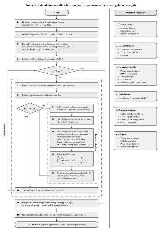
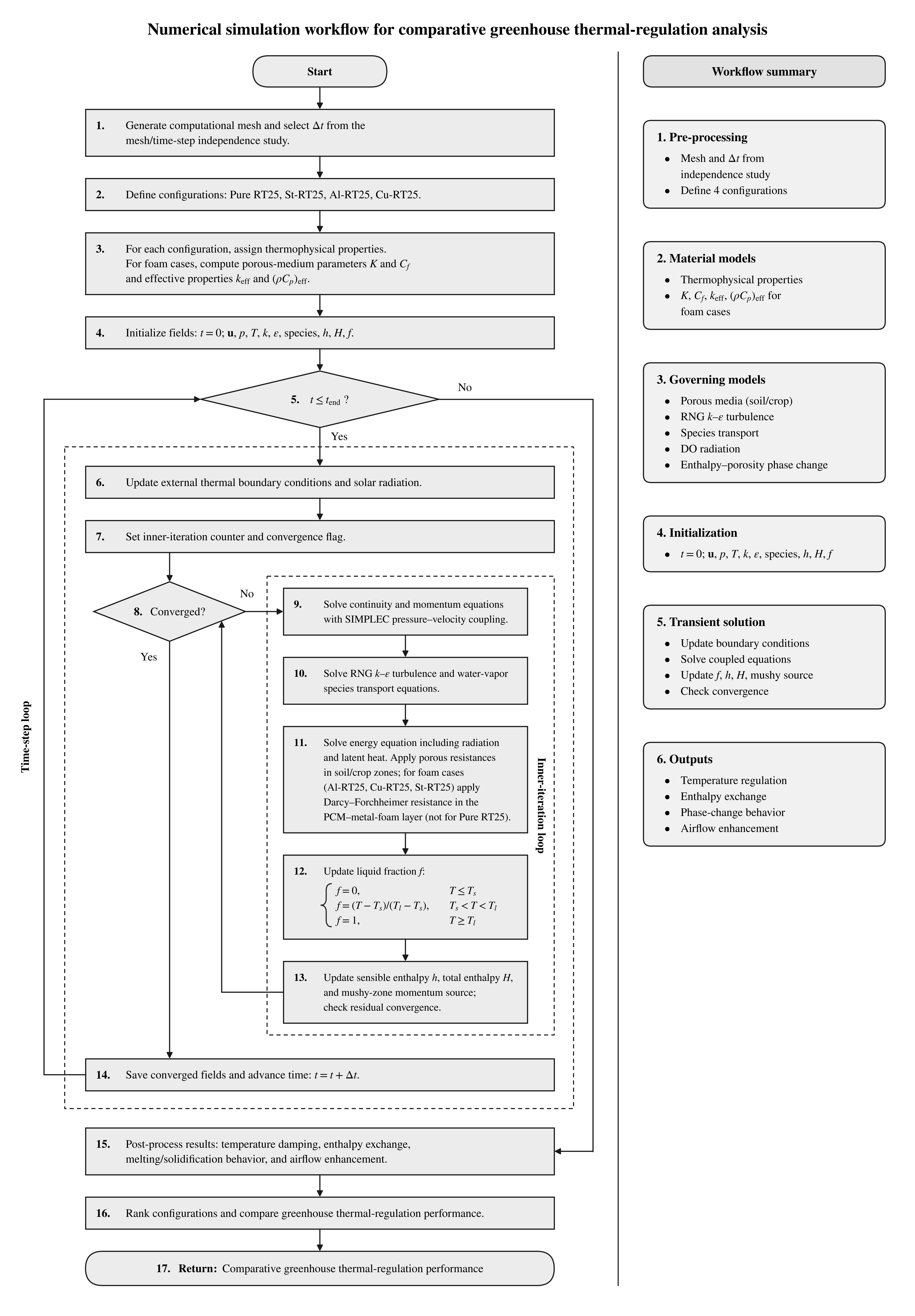
Figure 1 summarizes the numerical procedure as a step-by-step workflow linking the governing equations to the coupled CFD solution sequence.

Figure 1. Flowchart of the numerical simulation procedure for comparative greenhouse thermal-regulation analysis.

At each time step, radiation, porous resistance, turbulence, vapor transport, phase change, mushy-zone damping and the effective composite properties are updated in a coupled manner until the convergence criteria are met.

Table 1 gives the density, thermal conductivity, specific heat, thickness and absorptivity of the envelope and domain materials: air, ground, canopy, glass and ash brick.

Table 1. Thermophysical properties of envelope materials of the greenhouses.

Material	Density (kg⋅m−3)	Thermal Conductivity (W⋅m−1⋅K−1)	Specific Heat Capacity (J⋅kg−1⋅K−1)	Thickness (mm)	Absorptivity α
Air	1.205	0.02	1013	-	-
Ground	1300	1.00	800	400	0.95
Canopy	700	0.17	2310	600	0.46
Glass	2700	0.76	840	4	UV; 0.05/PAR; 0.1/NIR; 0.2
Ash brick	1700	0.81	989	400	-

The coordinates of the temperature monitoring points are listed in Table 2. The points are distributed over the greenhouse air space, the PCM layer, the ash-brick wall and the ground, at several heights and horizontal positions, so that the thermal state of the air, the walls, the soil and the crop zone can be followed in detail.

Table 2. Coordinates of temperature monitoring points in the greenhouse.

Greenhouse	Point 1	Point 2	Point 3	Point 4	Point 5	Point 6	Point 7	Point 8	Point 9	Point 10	Point 11
X (m)	0.95	0.95	0.95	0.95	0.95	2.95	4.95	2.6	7.9	7.9	6.2
Y (m)	0.7	1	1.8	2.6	3.4	1.8	1.8	2.95	0.7	1	1.8
	PCM			Ash brick
	Point 12	Point 13	Point 14	Point 15	Point 16	Point 17
X (m)	0.45	0.45	0.45	0.2	0.2	0.2
Y (m)	0.5	1.8	3.1	0.5	1.8	3.1
Ground	Point 18	Point 19	Point 20	Point 21	Point 22
X (m)	0.95	1.95	4.45	6.90	7.90
Y (m)	0.2	0.2	0.2	0.2	0.2

Table 3 lists the thermophysical properties of the candidate PCMs (capric/lauric acid, KF·4H₂O, PEG600, SP21EK and RT25) and of the three foam metals. The candidates differ in density, conductivity, specific heat, latent heat and phase-change temperature. RT25 was retained for the simulations because its melting range (25–26 °C) lies within the target greenhouse air-temperature band and, as a paraffin, it is chemically stable and compatible with the metal foams.

Table 3. Thermophysical properties of chosen materials as PCM and metal foams [33,34,35,36].

Material	Density (kg⋅m−3)	Thermal Conductivity (W⋅m−1⋅K−1)	Specific Heat Capacity (J⋅kg−1⋅K−1)	Latent Heat (J⋅kg−1)	Phase Change Temperature (°C)
Capric/Lauric Acid	900	0.14	1900	140,800	18
KF·4H2O	1450	0.56	2200	200,000	18
PEG600	960	0.23	2090	128,000	25
SP21EK	1200	0.5	2000	170,000	22
RT25	770	0.2	2000	180,000	25–26
Aluminum	2719	202.4	871	-	-
Steel	7830	13	468	-	-
Copper	8933	401	381	-	-

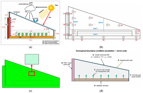
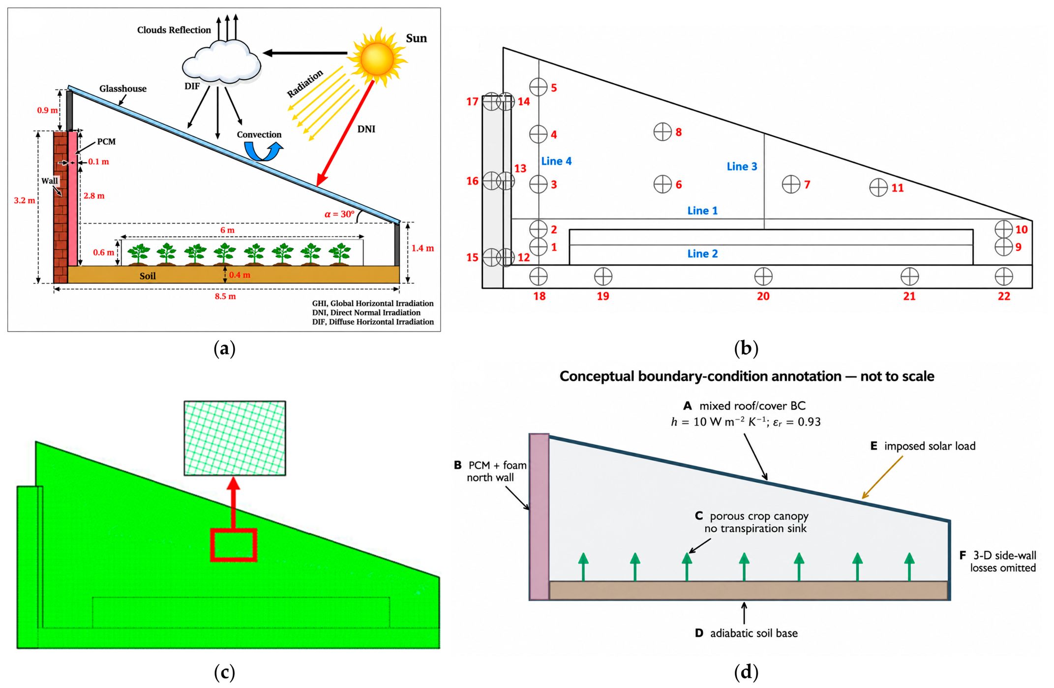
Figure 2 presents the greenhouse configuration, temperature-monitoring locations, computational mesh, and boundary-condition assumptions adopted in the numerical model. Figure 2a illustrates the greenhouse geometry, including its principal dimensions, inclined glazing, north-wall assembly containing the phase change material (PCM), crop region, soil layer, and incident solar radiation. Figure 2b identifies the 22 temperature-monitoring points and four monitoring lines used to evaluate the thermal response of the greenhouse, while Figure 2c shows the computational mesh, including an enlarged view of the local cell arrangement.

Figure 2. Overview of the greenhouse configuration and numerical model: (a) greenhouse geometry, principal dimensions, and incident solar radiation; (b) temperature-monitoring points and lines; (c) computational mesh with an enlarged view of the local cell arrangement; and (d) conceptual illustration of the boundary conditions and modeling assumptions, including omitted physical effects.

The monitoring locations were selected to characterize the temperature distribution within the greenhouse air space and surrounding materials, including the wall, PCM layer, ash brick, and soil. This arrangement enables the assessment of both short-term air-temperature variations and the delayed thermal response associated with heat storage in the surrounding materials.

Figure 2d provides a conceptual overview of the boundary conditions and modeling assumptions: (A) combined convective and radiative heat exchange at the exterior roof surface; (B) the north-wall PCM–foam assembly and its conjugate heat-transfer interface; (C) the crop canopy represented as a porous resistance without a calibrated transpiration sink; (D) the soil region with an adiabatic base; (E) the imposed solar load; and (F) out-of-plane heat exchange through the east and west side walls, which is omitted in the two-dimensional model. The diagram is schematic and not to scale, and distinguishes the imposed boundary conditions from physical processes excluded from the simulations.

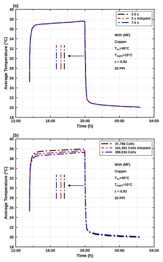
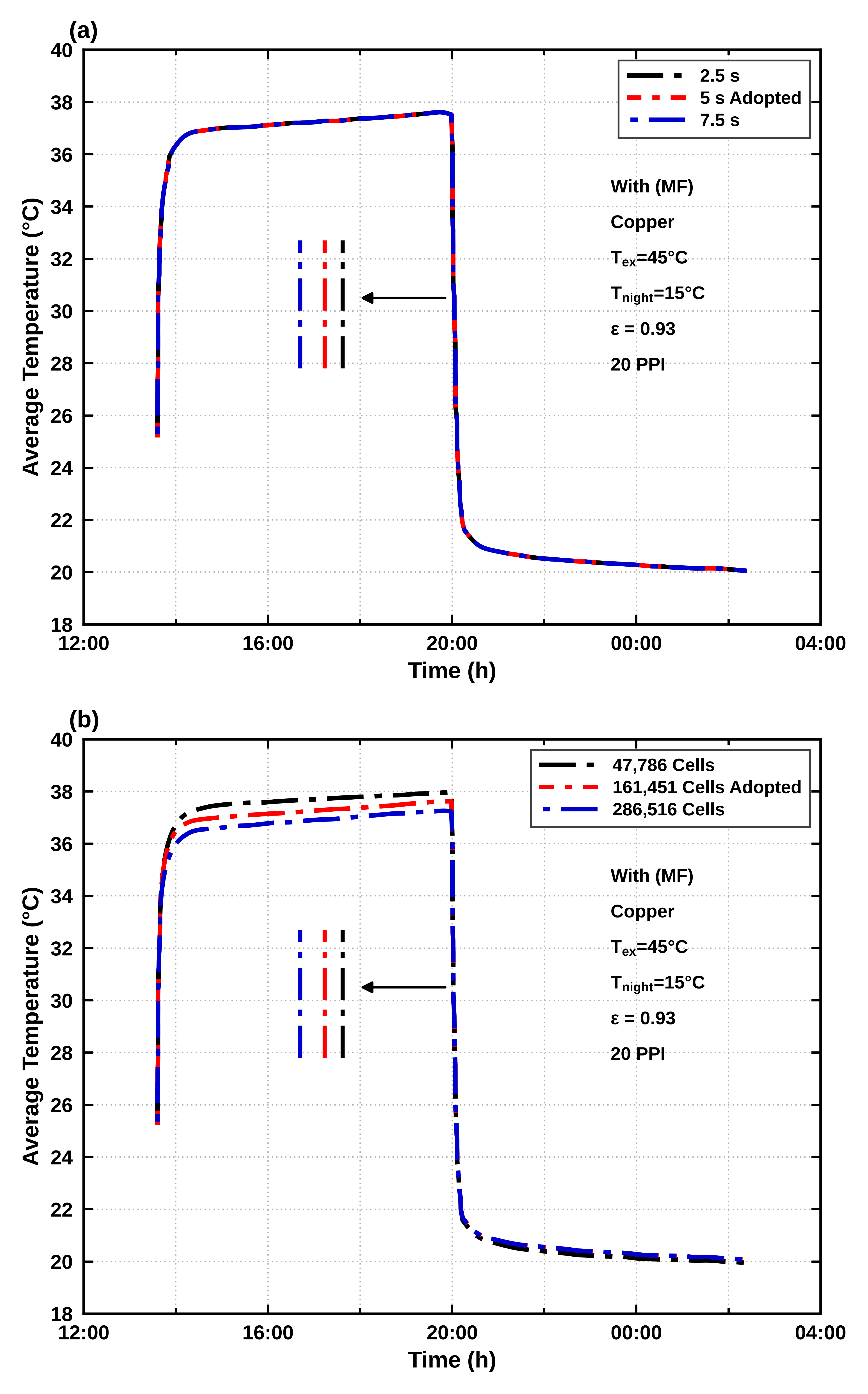
Figure 3 shows the volume-averaged temperature computed for the Cu–RT25 case using three time steps (2.5, 5, and 7.5 s) and three meshes (47,786, 161,451, and 286,516 cells). Table 4 lists the approximate deviations read from these curves at hourly instants during the daytime plateau (15:00–19:00) and the nighttime period (21:00–02:00). Because a relative temperature deviation requires an absolute temperature scale, the relative deviation is calculated using the adopted temperature in kelvins:

$${\delta }_T\left(\%\right)=100 |T-T_{\mathit{adopted}}|/T_{\mathit{adopted},K},\hspace{1em}\mathrm{where} T_{\mathit{adopted},K}=T_{\mathit{adopted}}\left(°\mathrm{C}\right)+273.15.$$

Figure 3. Sensitivity of the computed volume-averaged temperature (Cu–RT25, T_ext = 45 °C, T_night = 15 °C, 20 PPI) to (a) time-step size and (b) mesh refinement.

Table 4. Temperature-based time-step and mesh sensitivity of the computed volume-averaged temperature (Cu–RT25, T_ext = 45 °C, T_night = 15 °C), read from Figure 3.

Study	Compared Cases	Max |ΔT|, Day (K)	Max δT, Day (%)	Max |ΔT|, Night (K)	Max δT, Night (%)
Time Step	2.5 s vs. 5 s (adopted)	<0.05	<0.02	<0.05	<0.02
Time Step	7.5 s vs. 5 s (adopted)	0.06	0.02	0.02	0.01
Mesh	47,786 vs. 161,451 cells (adopted)	0.46	0.15	0.19	0.06
Mesh	286,516 vs. 161,451 cells (adopted)	0.39	0.13	0.07	0.02

The reading resolution of the plots is approximately 0.05 °C. The time-step curves are practically superimposed. Between the adopted 5 s time step and the 7.5 s time step, the maximum temperature differences are approximately 0.06 K during the daytime period and 0.02 K during the nighttime period, corresponding to approximately 0.02% and 0.01%, respectively. The 2.5 s curve differs from the 5 s curve by less than the approximate reading resolution of the plot. Refining the mesh from 47,786 to 161,451 cells changes the temperature by up to approximately 0.46 K during the day and 0.19 K at night, corresponding to approximately 0.15% and 0.06%, respectively. Further refinement from 161,451 to 286,516 cells changes the temperature by up to approximately 0.39 K during the day and 0.07 K at night, corresponding to approximately 0.13% and 0.02%, respectively. The 161,451-cell mesh and the 5 s time step were therefore retained as a compromise between the observed temperature sensitivity and computational cost.

This numerical-sensitivity assessment is limited to the computed volume-averaged temperature, which was the common global response variable recorded for all mesh and time-step cases. Matched sensitivity histories for air velocity, wall heat flux, and PCM liquid fraction were not retained and cannot be reconstructed reliably from production-case profiles or snapshots obtained under different sampling or boundary conditions. Consequently, the present analysis supports the adopted numerical resolution for the reported volume-averaged temperature response but does not establish variable-specific numerical independence for the other reported fields.

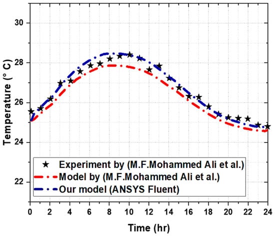
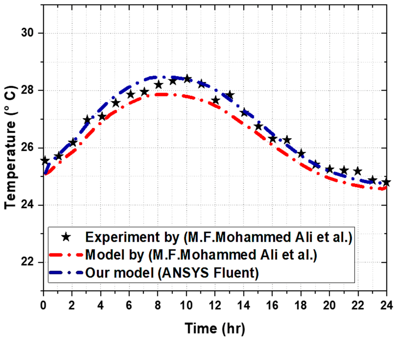
Figure 4 compares the 24 h inner roof-surface temperature predicted by the present CFD model for the HASP–GW benchmark using PCM1 43–47 °C with the corresponding experimental measurements and numerical results reported by Mohammed Ali et al. [37]. The reference experiment concerns the interior surface of an active building-roof slab incorporating external PCM panels and embedded water pipes supplied by a geothermal source. The experimental system differs from the present greenhouse configuration in geometry, PCM operating conditions, airflow and thermal boundary conditions, and in the absence of crops, a radiative greenhouse enclosure, and a metal-foam composite. The comparison therefore evaluates only the ability of the adopted CFD approach to reproduce the transient inner roof-surface temperature under the benchmark conditions. It does not validate greenhouse radiation, humidity, turbulence, crop-canopy effects, or foam–PCM coupling and is therefore regarded as a limited thermal benchmark rather than validation of the complete system.

Figure 4. Comparison of the 24 h inner roof-surface temperature of the HASP–GW system with PCM1: experimental measurements and numerical predictions reported by Mohammed Ali et al. [37], and predictions from the present ANSYS Fluent model. This benchmark does not validate the complete greenhouse–metal-foam physics.

Agreement was evaluated at 25 hourly points (N = 25) digitized from the published experimental and numerical curves. The metrics were calculated as RMSE = [(1/N)Σ(T_CFD,i − T_exp,i)²]^1/2, MAE = (1/N)Σ|T_CFD,i − T_exp,i|, the maximum absolute deviation, and the coefficient of determination R². As listed in Table 5, the present benchmark simulation gives RMSE = 0.21 °C, MAE = 0.16 °C, a maximum absolute deviation of 0.44 °C, and R² = 0.97. The maximum deviation occurs at t = 0 h and reflects the imposed initial condition. Using the same experimental points, the numerical curve presented by Mohammed Ali et al. [37] yields RMSE = 0.40 °C and MAE = 0.37 °C. Because the values were digitized from published curves, the resulting metrics are approximate. Subject to the scope limitations stated above, the comparison supports the PCM-related temperature response to within approximately 0.5 °C.

Table 5. Agreement between predicted and measured inner roof-surface temperatures for the HASP–GW benchmark of Figure 4 (N = 25 hourly points).

Model	RMSE (°C)	MAE (°C)	Max |ΔT| (°C)	R2
Present CFD model (ANSYS Fluent)	0.21	0.16	0.44	0.97
Numerical model of Mohammed Ali et al. [37]	0.40	0.37	0.68	0.89

4. Results and Discussion

The results are presented in the following sequence: local heat exchange at the greenhouse glass surface, temperature distributions within the greenhouse and surrounding materials, PCM melting and solidification behavior, and local airflow characteristics. This organization facilitates the interpretation of the coupled thermal processes and their influence on greenhouse temperature regulation. In particular, heat conduction through the PCM–metal-foam layer, buoyancy-driven convection, and latent heat storage are interconnected mechanisms that influence the overall thermal response. However, temperature variations, phase-change behavior, and local air velocity represent distinct performance indicators and should not be interpreted independently as measures of energy efficiency. The pure-RT25 configuration provides the baseline for material comparisons under identical boundary forcing, evaluation interval, and monitoring location. The air-temperature excursion is defined as

$$\mathsf{\Delta }{T}_{\mathrm{a}\mathrm{i}\mathrm{r}}=\underset{t}{\max }\left[T_{\mathrm{a}\mathrm{i}\mathrm{r}}\left(t\right)\right]-\underset{t}{\min }\left[T_{\mathrm{a}\mathrm{i}\mathrm{r}}\left(t\right)\right],$$

with the reduction relative to pure RT25 given by

$$\mathsf{\Delta }\left(\mathsf{\Delta }{T}_{\mathrm{a}\mathrm{i}\mathrm{r}}\right)=\mathsf{\Delta }{T}_{\mathrm{a}\mathrm{i}\mathrm{r},\mathrm{p}\mathrm{u}\mathrm{r}\mathrm{e}}-\mathsf{\Delta }{T}_{\mathrm{a}\mathrm{i}\mathrm{r},\mathrm{f}\mathrm{o}\mathrm{a}\mathrm{m}}.$$

A positive value therefore indicates a reduction in the temperature excursion. At a specified surface and time, and provided that $\left|{\dot{Q}}_{\mathrm{p}\mathrm{u}\mathrm{r}\mathrm{e}}\right|$ is not close to zero, the heat-flow enhancement may be evaluated as

$$G_Q\left(\%\right)=100{\displaystyle \frac{{\dot{Q}}_{\mathrm{f}\mathrm{o}\mathrm{a}\mathrm{m}}-{\dot{Q}}_{\mathrm{p}\mathrm{u}\mathrm{r}\mathrm{e}}}{\left|{\dot{Q}}_{\mathrm{p}\mathrm{u}\mathrm{r}\mathrm{e}}\right|}}.$$

The corresponding time-integrated heat-transfer indicator is

$$E_Q={\int }_{t_1}^{t_2}\dot{Q}\hspace{0.17em}dt,$$

evaluated over the same time interval for all configurations. These indicators must be distinguished from stored enthalpy and local air velocity, which quantify different aspects of the thermal response.

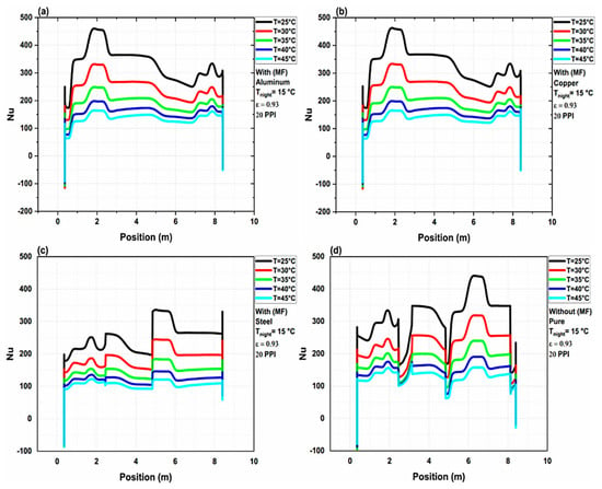
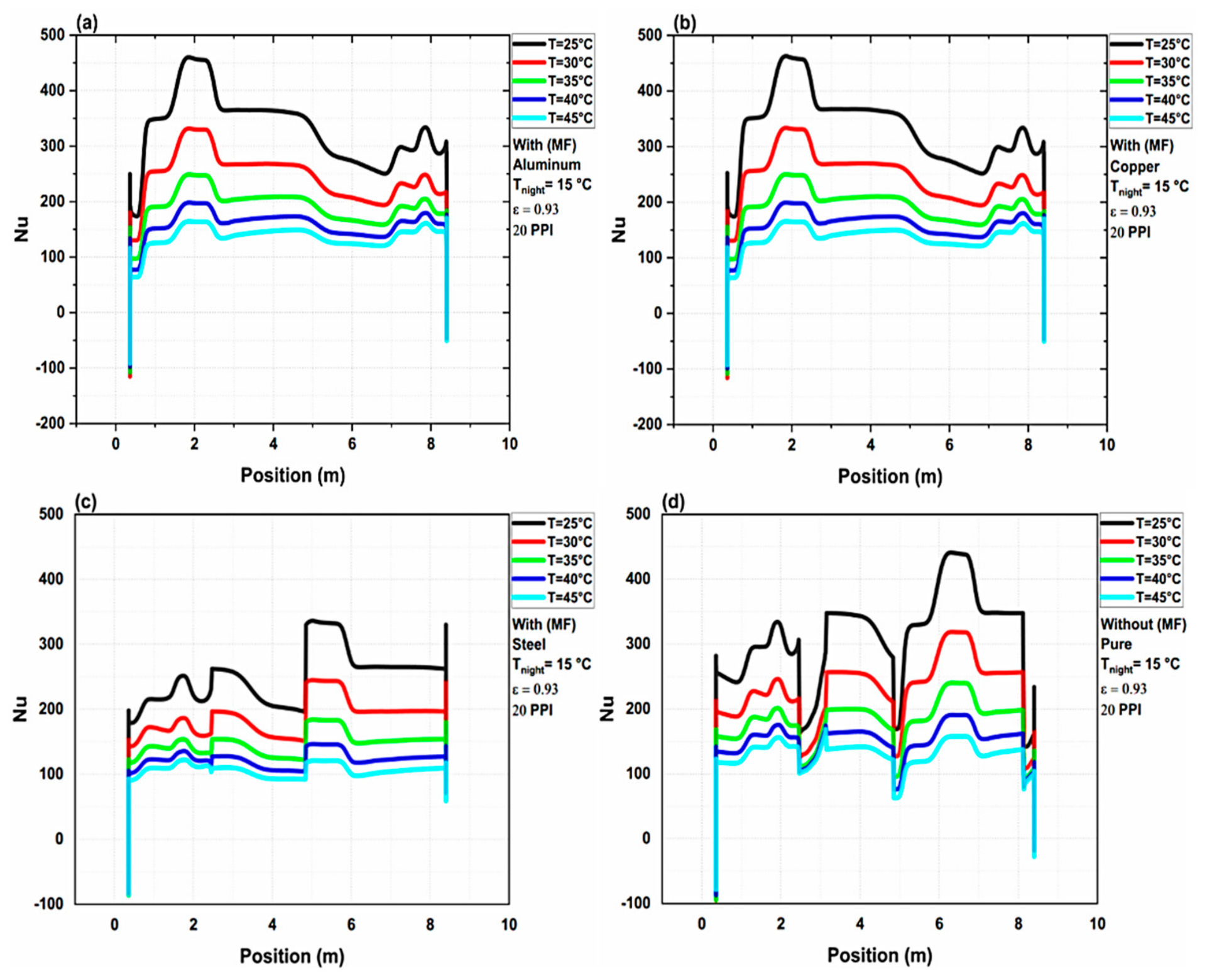
Figure 5 presents the local Nusselt number as a function of position along the glass facade, sampled at t = 10,000 s. This is a spatial distribution rather than a time-history graph. Local peaks indicate relatively stronger convective exchange but do not by themselves provide an integrated heat-transfer-rate or energy-savings percentage.

Figure 5. Spatial distribution of the local Nusselt number along the greenhouse glass façade at t = 10,000 s for (a) RT25 embedded in aluminum foam (Al–RT25); (b) RT25 embedded in copper foam (Cu–RT25); (c) RT25 embedded in steel foam (St–RT25); and (d) pure RT25 without metal foam.

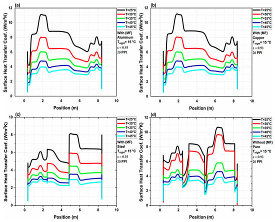
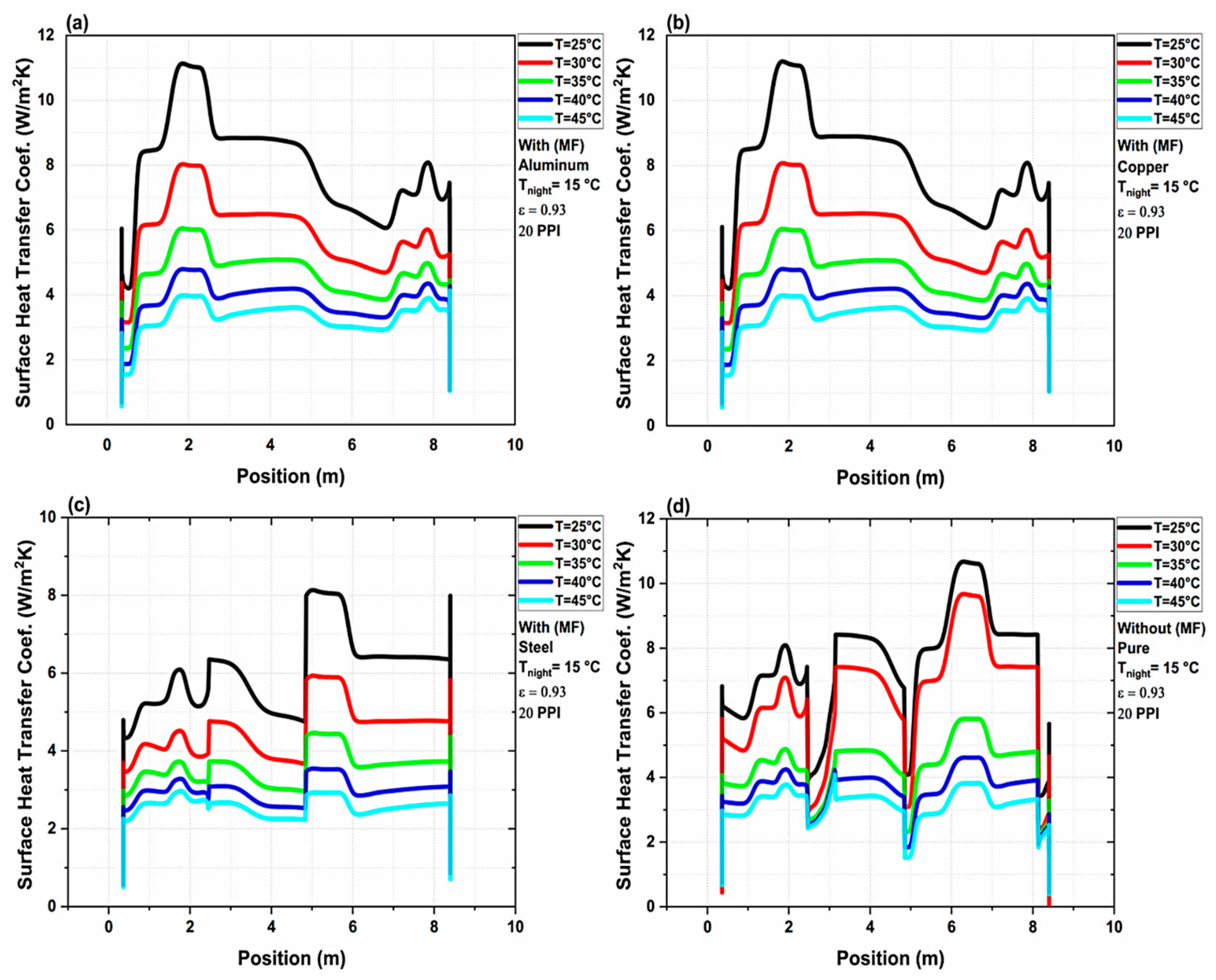
Figure 6 shows the local convective heat-transfer coefficient h(x) (W m⁻² K⁻¹) along the glass façade at the same time. Like Figure 5, it is a spatial profile: the horizontal axis is position along the façade, not time. The coefficient reaches a maximum of about 11 W m⁻² K⁻¹; the whole-façade heat transfer would require integrating the local heat flux over the surface, so neither figure alone quantifies daily energy savings.

Figure 6. Spatial distribution of the local convective heat-transfer coefficient, h(x) (W m⁻² K⁻¹), along the greenhouse glass façade at t = 10,000 s for (a) RT25 embedded in aluminum foam (Al–RT25); (b) RT25 embedded in copper foam (Cu–RT25); (c) RT25 embedded in steel foam (St–RT25); and (d) pure RT25 without metal foam.

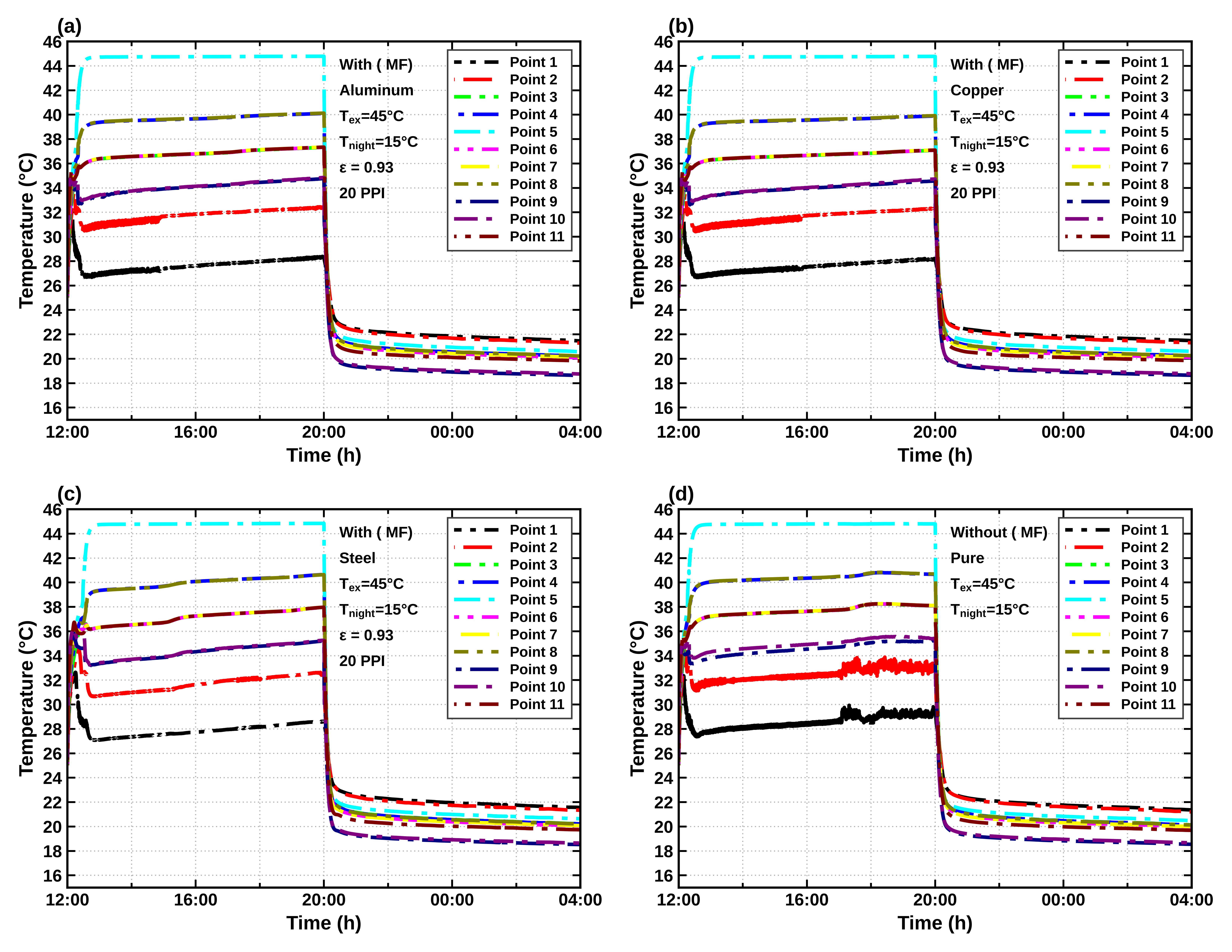
Figure 7 compares the greenhouse air-temperature responses of the PCM/foam configurations under T_ext = 45 °C and T_night = 15 °C. The pure-RT25 profile is the reference for judging any reduction in peak temperature or thermal excursion. The traces show a material-dependent redistribution of heat; temperature differences between configurations are meaningful only when taken at the same sensor, time and forcing condition.

Figure 7. Greenhouse air-temperature profiles at monitoring points 1–11 for (a) RT25 embedded in aluminum foam (Al–RT25); (b) RT25 embedded in copper foam (Cu–RT25); (c) RT25 embedded in steel foam (St–RT25); and (d) pure RT25 without metal foam. Simulation conditions: T_ext = 45 °C, T_night = 15 °C, and ε_rad = 0.93, with a foam pore density of 20 PPI for the metal-foam configurations. The pure-RT25 configuration serves as the reference case for comparing temperature responses under identical conditions.

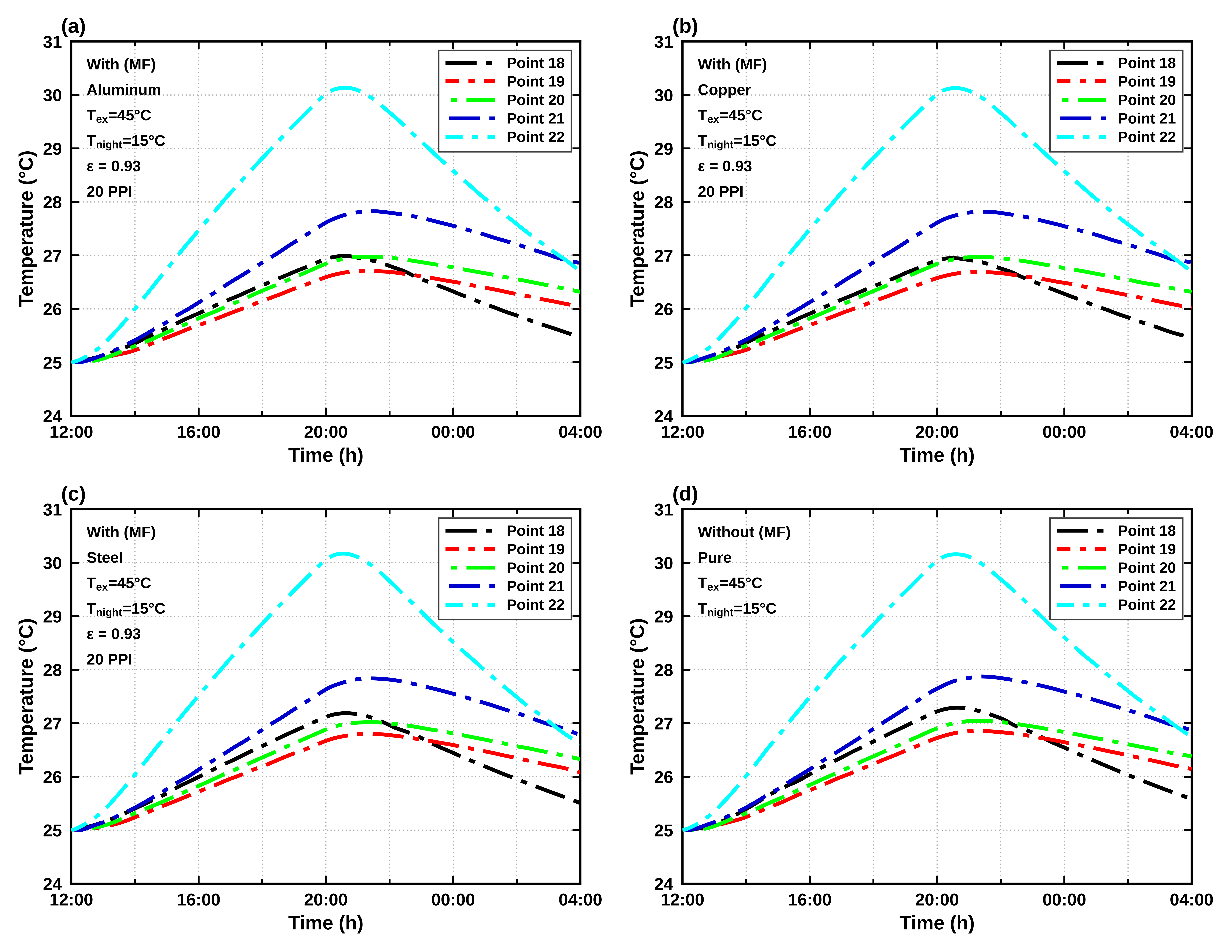
Figure 8 illustrates the effect of the PCM–foam layer on the ground-temperature response for the stated 15 °C nighttime case. Thermal coupling among wall, air and soil explains the sensitivity of this field to material conductivity and stored heat. The magnitude of any ground-temperature benefit should be computed from matched location/time pairs and is not converted here into separately validated energy saving.

Figure 8. Ground-temperature profiles at monitoring points 18–22 for (a) RT25 embedded in aluminum foam (Al–RT25); (b) RT25 embedded in copper foam (Cu–RT25); (c) RT25 embedded in steel foam (St–RT25); and (d) pure RT25 without metal foam. Simulation conditions: T_ext = 45 °C, T_night = 15 °C, and ε_rad = 0.93, with a foam pore density of 20 PPI for the metal-foam configurations. The pure-RT25 configuration serves as the reference case for comparing ground-temperature responses under identical conditions.

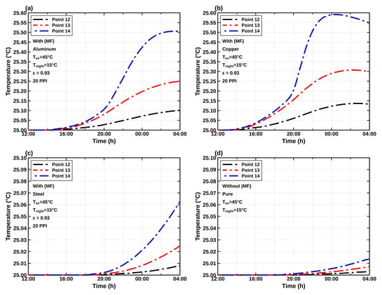
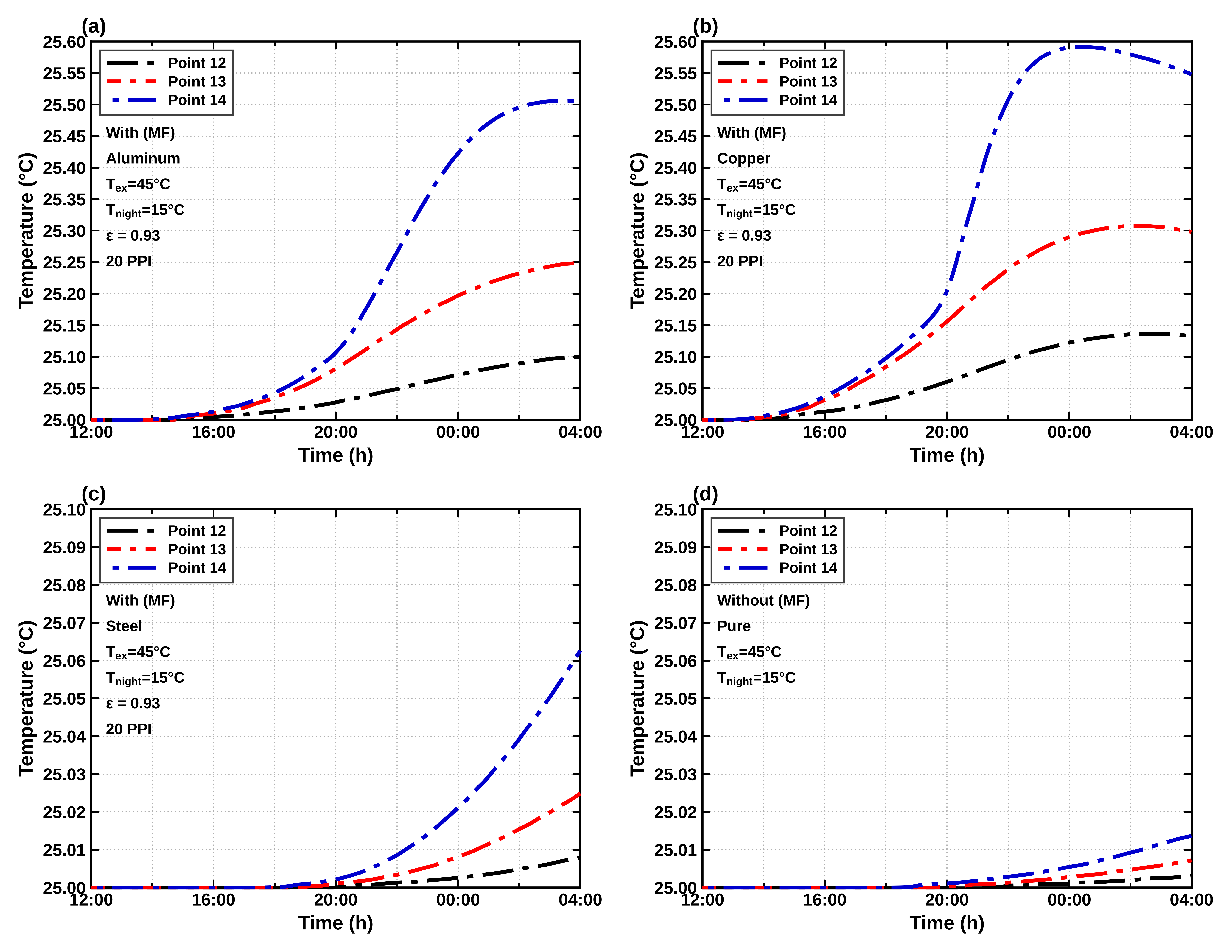
Figure 9 displays the PCM–metal-foam temperature profiles for the 45 °C/15 °C thermal scenario and the selected 20 PPI condition. Material-dependent wall-temperature attenuation is evident in the plotted traces, but the ordering depends on whether one examines a peak, time average, PCM sensor temperature or heat-transfer quantity. Differences are therefore discussed by plot-specific measurement rather than declaring aluminum or copper universally superior in all thermal criteria.

Figure 9. Temperature profiles at the PCM monitoring points for (a) RT25 embedded in aluminum foam (Al–RT25); (b) RT25 embedded in copper foam (Cu–RT25); (c) RT25 embedded in steel foam (St–RT25); and (d) pure RT25 without metal foam. Simulation conditions: T_ext = 45 °C, T_night = 15 °C, and ε_rad = 0.93, with a foam pore density of 20 PPI for the metal-foam configurations.

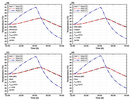
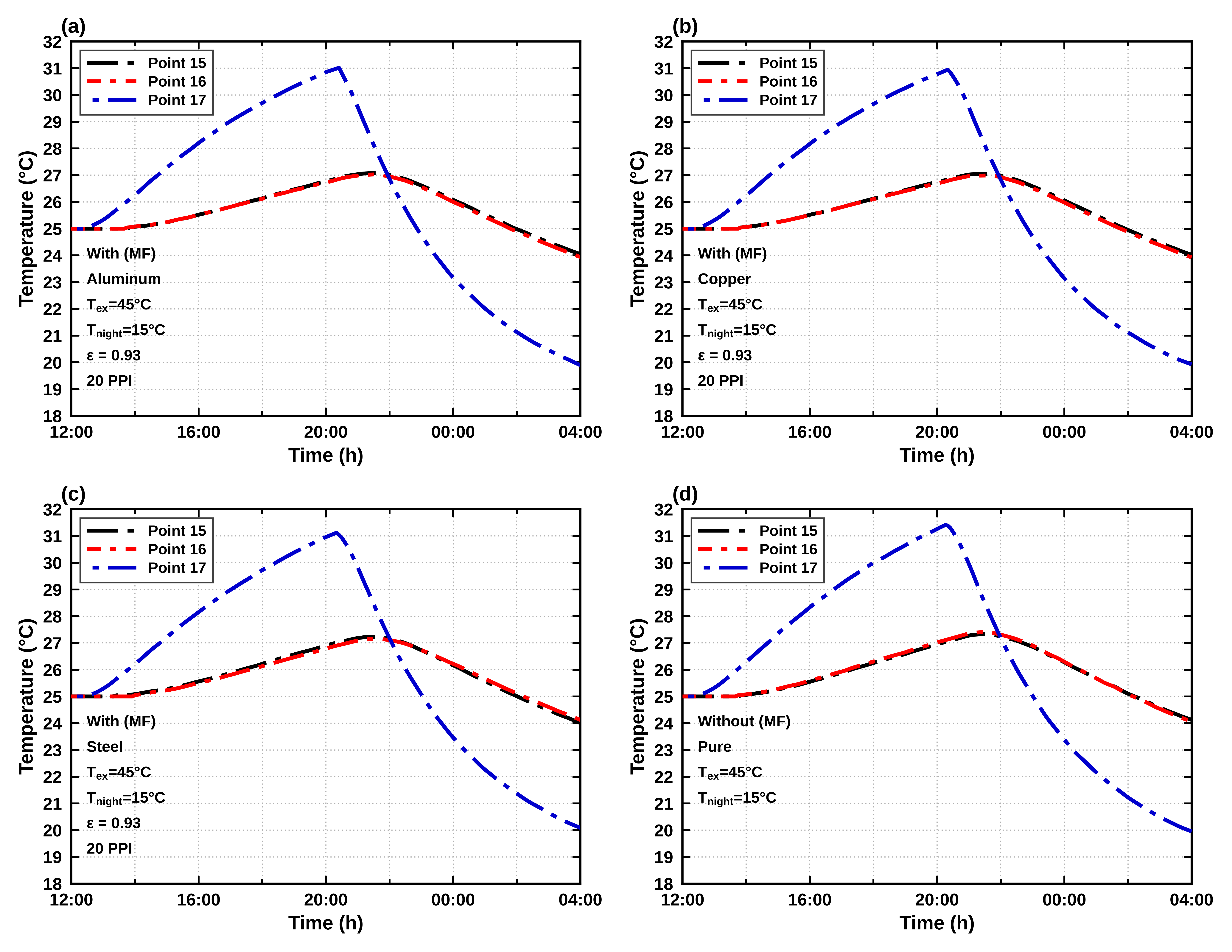
Figure 10 compares the temperature histories of the ash-brick zone under the reported 45 °C/15 °C thermal condition. Differences among Cu–RT25, Al–RT25, St–RT25 and pure RT25 are consistent with altered thermal spreading from the adjacent storage layer. The ash-brick trace is not a direct measurement of crop energy consumption, and a rank for this location does not establish an overall system efficiency or economic optimum.

Figure 10. Ash-brick temperature profiles at monitoring points 15–17 for (a) RT25 embedded in aluminum foam (Al–RT25); (b) RT25 embedded in copper foam (Cu–RT25); (c) RT25 embedded in steel foam (St–RT25); and (d) pure RT25 without metal foam. Simulation conditions: T_ext = 45 °C, T_night = 15 °C, and ε_rad = 0.93, with a foam pore density of 20 PPI for the metal-foam configurations.

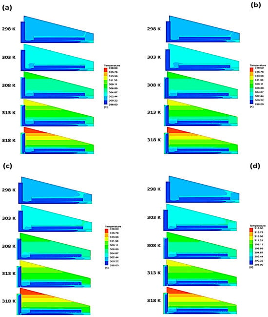
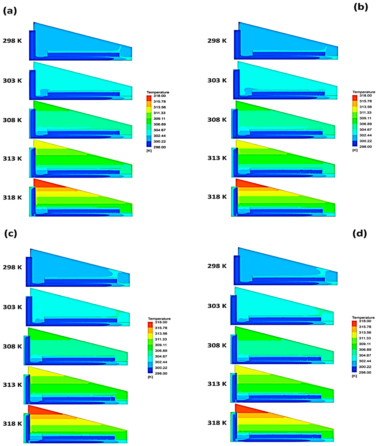
Figure 11 shows the temperature field in the greenhouse at t = 28,000 s for each material. Differences in conductivity redistribute heat within the storage wall, although the contour maps cannot by themselves separate the contributions of conduction, natural convection and phase change.

Figure 11. Temperature contours for (a) aluminum, (b) copper, (c) steel and (d) pure RT25 at t = 28,000 s; T_ext = 45 °C, T_night = 15 °C, ε_rad = 0.93, selected foam of 20 PPI.

The incorporation of metal foam influences three coupled heat-transfer mechanisms that should be distinguished when interpreting the thermal response of the greenhouse. First, the metal skeleton modifies conductive heat transport within the PCM layer, which can be characterized by the local conductive heat flux,

$${q″}_{\mathrm{c}\mathrm{o}\mathrm{n}\mathrm{d}}=-k_{\mathrm{e}\mathrm{f}\mathrm{f}}\nabla T\cdot \mathbf{n}.$$

Second, the resulting changes in temperature distribution may alter buoyancy-driven airflow and convective heat transport within the greenhouse. Third, changes in heat distribution influence PCM melting and solidification, with the stored latent energy expressed as

$$E_{\mathrm{l}\mathrm{a}\mathrm{t}}\left(t\right)={\int }_V{\epsilon }_p{\rho }_{\mathrm{P}\mathrm{C}\mathrm{M}}Lf\left(t\right)\hspace{0.17em}dV,$$

where ${\epsilon }_p$ is the PCM volume fraction, ${\rho }_{\mathrm{P}\mathrm{C}\mathrm{M}}$ is the PCM density, L is the latent heat of fusion, and f is the liquid fraction. The corresponding rate of latent-energy storage or release depends on the temporal change in E_lat. These mechanisms are interconnected, and the temperature distributions presented in Figure 11 do not independently establish their respective contributions to the overall thermal response. A quantitative decomposition would require additional controlled simulations under identical initial and boundary conditions, systematically varying the conductive, convective, and phase-change contributions while accounting for their interactions.

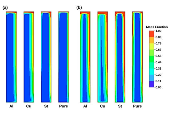
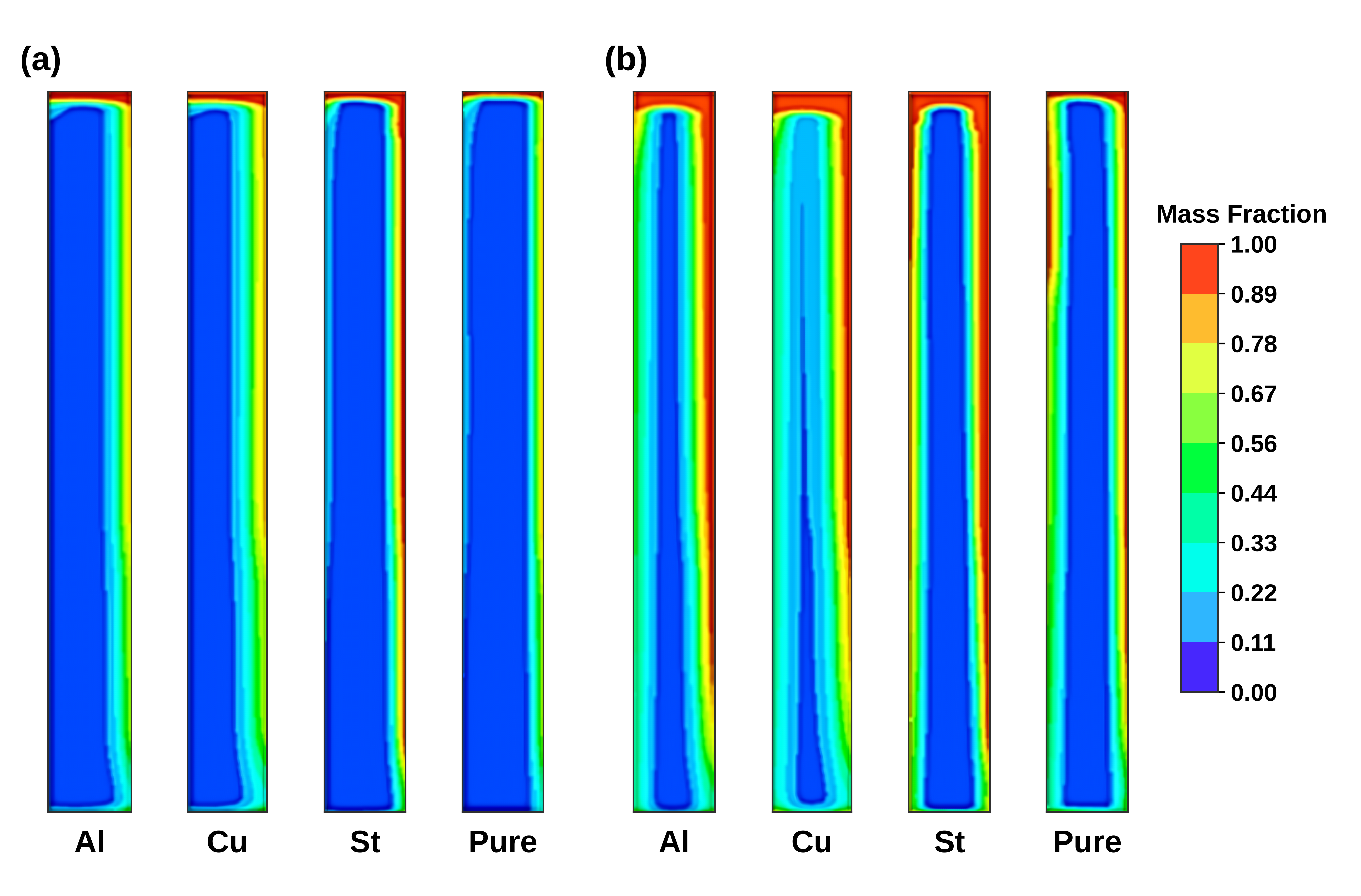
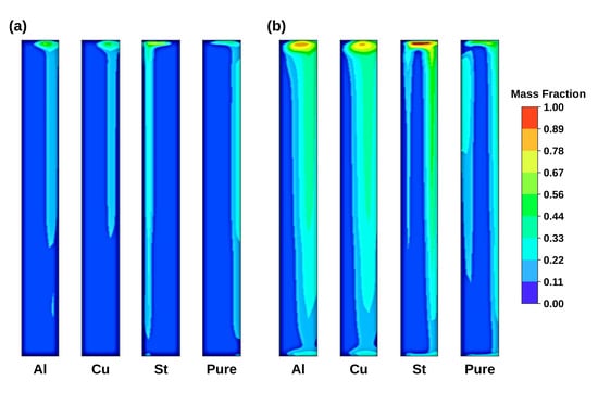
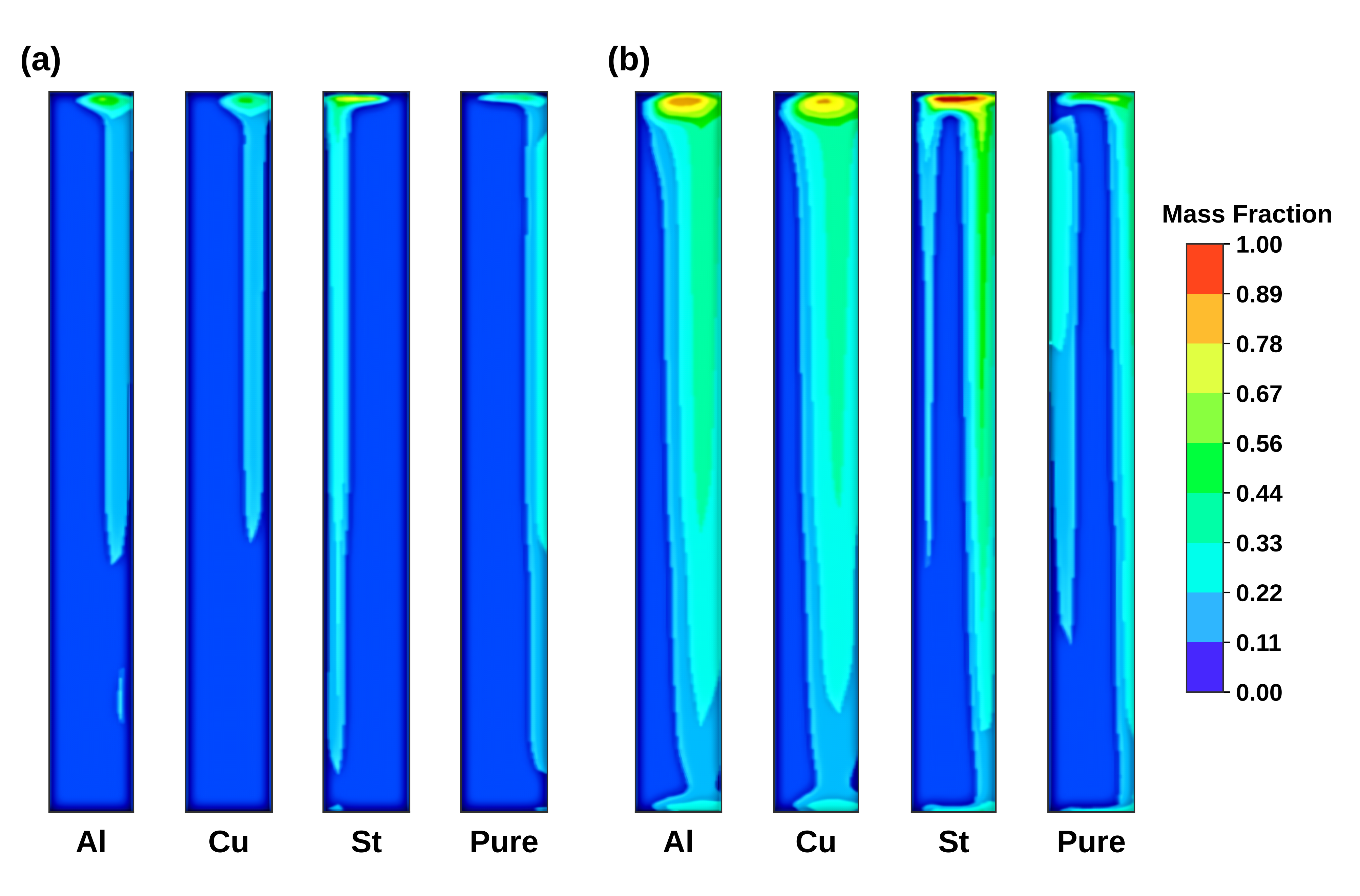
Figure 12 presents the PCM liquid fraction at t = 28,000 s for the two imposed daytime conditions, with T_night = 15 °C. The warmer case shows a larger melted region. Liquid fraction is a dimensionless indicator of the storage state; the usable recovered energy also depends on the PCM mass, the latent heat and the subsequent solidification, so a single snapshot does not provide an integrated heat-transfer rate.

Figure 12. PCM liquid-fraction fields during melting at t = 28,000 s for (a) T_ext = 25 °C and (b) T_ext = 45 °C, both with T_night = 15 °C and selected foam of 20 PPI.

Figure 13 shows the solidification response for the two daytime conditions with a 15 °C night setting. The plotted quantity is the local solid fraction, 1 − f. The fields indicate different degrees of regeneration after charging, but performance over repeated day–night cycles cannot be inferred from a single cycle.

Figure 13. PCM solid-fraction fields during solidification at t = 57,000 s for (a) T_ext = 25 °C and (b) T_ext = 45 °C, both with T_night = 15 °C and selected foam of 20 PPI.

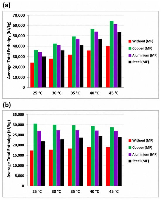
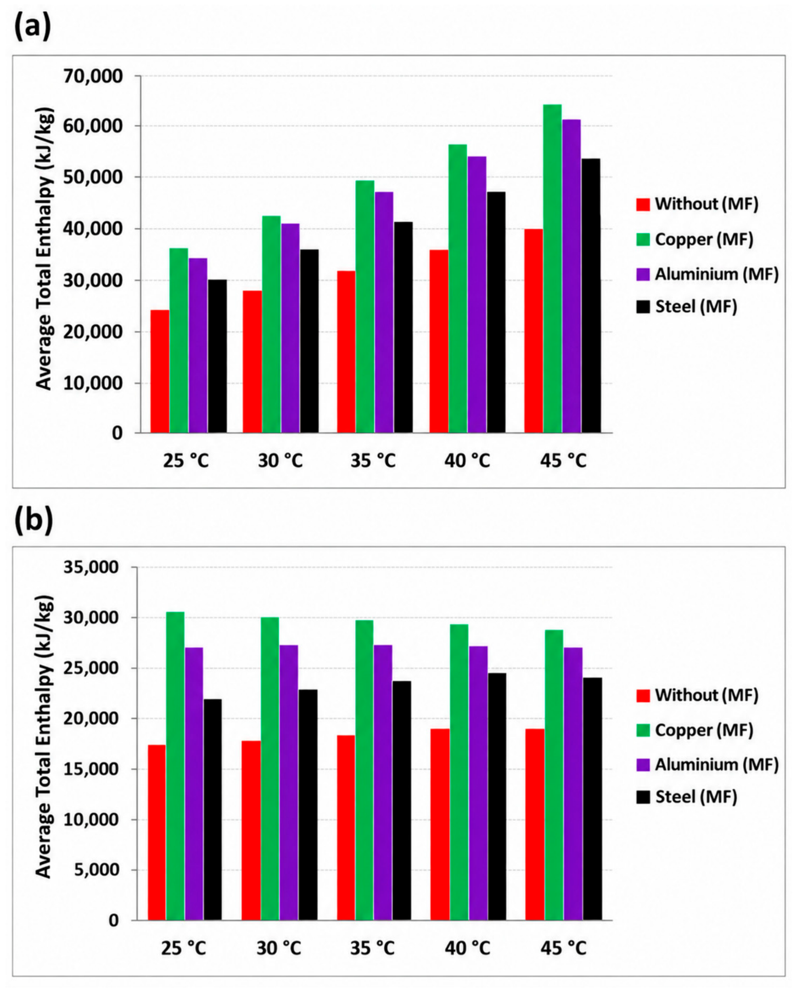
Figure 14 shows the enthalpy of the PCM/foam systems during melting and solidification. In both panels, the copper-foam composite reaches larger enthalpy values than the aluminum-foam composite. An enthalpy value alone, however, neither measures charging or recovery efficiency nor indicates faster heat exchange; such indicators require normalization by composite mass or volume and by time, together with a defined ratio of useful recovered heat to supplied heat over matched operating intervals.

Figure 14. Mean enthalpy of the PCM/foam configurations versus temperature during (a) melting and (b) solidification; T_ext = 45 °C, T_night = 15 °C, selected foam of 20 PPI, pore fraction ε_p = 0.91 and applied heat flux q″ = 610 W m⁻².

The ranking of the materials depends on the quantity being evaluated. Copper has the highest constituent thermal conductivity in Table 3, but conductivity is a material property rather than a complete system-performance indicator. In Figure 9, the PCM temperatures are compared only at the same monitoring point, time, and boundary condition relative to pure RT25. In Figure 14, Cu–RT25 has higher plotted mean enthalpy than Al–RT25 at each evaluated temperature 25, 30, 35, 40, and 45 °C during both melting and solidification. Aluminum therefore cannot be described as having the highest enthalpy-exchange efficiency. An enthalpy value alone does not quantify charging or recovery efficiency, which would require normalization of the useful stored or recovered energy by the supplied energy over a matched operating interval.

The present simulations characterize the PCM thermal response under the prescribed operating conditions but do not establish its performance over consecutive day–night cycles. During repeated operation, incomplete nighttime solidification may leave a residual liquid fraction at the beginning of the following day, reducing the latent heat storage capacity available for subsequent charging. Conversely, incomplete daytime melting indicates that part of the available latent storage capacity remains unused. These effects may influence the daily thermal response and the effectiveness of the PCM storage system over successive cycles. A comprehensive assessment of long-term cyclic performance would require monitoring the volume-averaged liquid fraction at the beginning and end of each cycle, the latent energy charged and discharged, the recovered-energy fraction, and the cycle-to-cycle evolution of PCM temperature and phase state. Since these quantities have not been evaluated over repeated cycles, no conclusions are drawn regarding long-term regeneration stability, cumulative performance attenuation, or seasonal thermal performance.

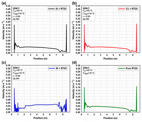
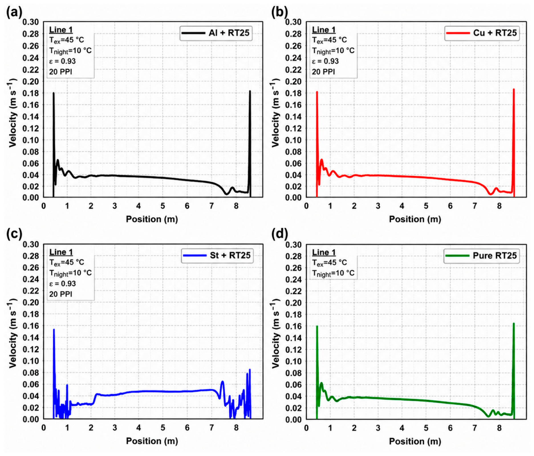
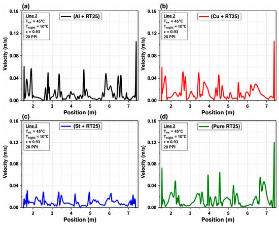
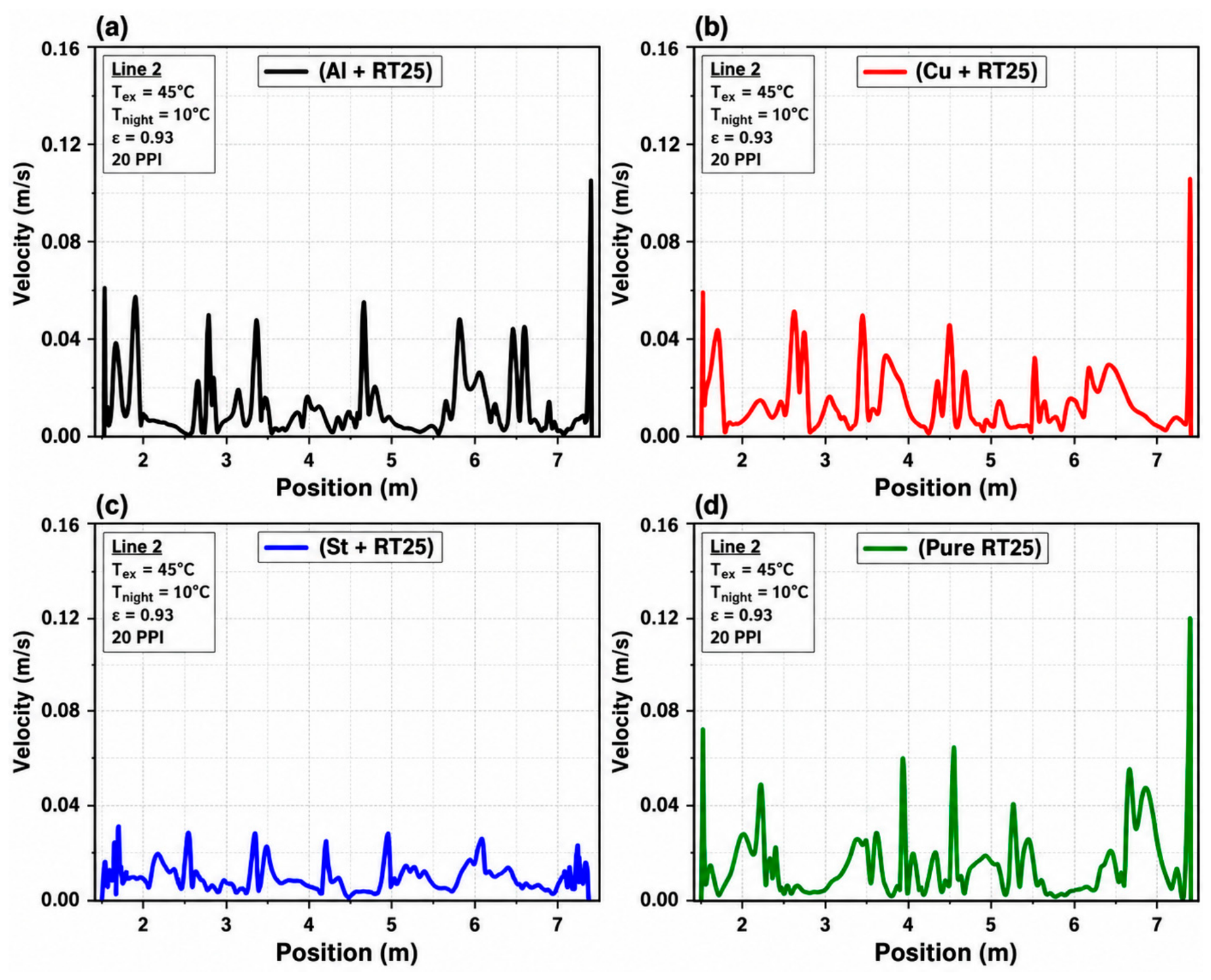
The local velocity profiles in Figure 15 and Figure 16 represent a separate airflow response and are not used to rank thermal-storage efficiency. Likewise, an economic advantage of aluminum cannot be established without data on foam mass, procurement, fabrication, encapsulation, installation, and lifetime cost.

Figure 15. Local greenhouse velocity profiles along horizontal line 1 for (a) Al–RT25, (b) Cu–RT25, (c) St–RT25 and (d) pure RT25 at t = 10,000 s, T_ext = 45 °C, T_night = 10 °C and selected foam of 20 PPI.

Figure 16. Local greenhouse velocity profiles along horizontal line 2 for (a) Al–RT25, (b) Cu–RT25, (c) St–RT25 and (d) pure RT25 at t = 10,000 s, T_ext = 45 °C, T_night = 10 °C and selected foam of 20 PPI.

Figure 15 presents the local velocity profiles along line 1 at t = 10,000 s for the 10 °C nighttime scenario. The differences among the curves reflect the combined influence of heat transfer and buoyancy-driven circulation rather than thermal conductivity alone. Any velocity enhancement must be evaluated relative to pure RT25 at the same sampling coordinate, time, and boundary condition. Because the profile maxima are approximately 0.19 m s⁻¹, the plots do not support the previously stated velocity increase of 0.3–0.5 m s⁻¹. Figure 16 presents a second velocity comparison along line 2 for the same 10 °C nighttime scenario, with profile maxima of approximately 0.12 m s⁻¹. As for Figure 15, any enhancement should be reported as a pointwise or line-averaged difference relative to pure RT25 under the same conditions. Because these profiles belong to the separate 10 °C airflow scenario, they are not combined quantitatively with the thermal and phase-change results obtained for the 15 °C nighttime scenario.

Figure 16 gives a second velocity comparison, along line 2, for the same 10 °C scenario, with maxima of about 0.12 m s⁻¹. As for Figure 15, any enhancement should be reported as a pointwise or line-averaged difference from pure RT25, and these profiles are not combined quantitatively with the thermal results obtained for the 15 °C scenario.

A change in passive greenhouse temperature does not by itself quantify a reduction in HVAC energy use. Such a calculation requires a defined reference system, thermostat set-points, an equipment operating schedule, and a time-resolved thermal-load balance. If ${\dot{Q}}_{\mathrm{r}\mathrm{e}\mathrm{q}}\left(t\right)$ denotes the net sensible power required to maintain the prescribed indoor condition, with positive values representing cooling demand, the peak sensible cooling power can be defined as

$$P_{\mathrm{c}\mathrm{o}\mathrm{o}\mathrm{l},\mathrm{p}\mathrm{e}\mathrm{a}\mathrm{k}}=\underset{t}{\max }\left[\max \left(0,{\dot{Q}}_{\mathrm{r}\mathrm{e}\mathrm{q}}\left(t\right)\right)\right],$$

the daily cooling energy as

$$E_{\mathrm{c}\mathrm{o}\mathrm{o}\mathrm{l}}={\int }_{\mathrm{d}\mathrm{a}\mathrm{y}}\max \left(0,{\dot{Q}}_{\mathrm{r}\mathrm{e}\mathrm{q}}\left(t\right)\right)\hspace{0.17em}dt,$$

and the percentage daily cooling-energy saving as

$$100{\displaystyle \frac{E_{\mathrm{c}\mathrm{o}\mathrm{o}\mathrm{l},\mathrm{p}\mathrm{u}\mathrm{r}\mathrm{e}}-E_{\mathrm{c}\mathrm{o}\mathrm{o}\mathrm{l},\mathrm{f}\mathrm{o}\mathrm{a}\mathrm{m}}}{E_{\mathrm{c}\mathrm{o}\mathrm{o}\mathrm{l},\mathrm{p}\mathrm{u}\mathrm{r}\mathrm{e}}}}.$$

Analogous definitions can be applied to the heating demand using the negative part of ${\dot{Q}}_{\mathrm{r}\mathrm{e}\mathrm{q}}\left(t\right)$. Since controlled HVAC demand histories were not computed for the analyzed cases, no cooling- or heating-load-reduction percentages are reported.

5. Conclusions and Limitations

This numerical comparison considered pure RT25 and aluminum-, copper- and steel-foam/RT25 layers for passive thermal management of a glass-roofed greenhouse. The analysis resolves illustrative temperature, enthalpy, liquid-fraction and flow responses under the specified two-dimensional models; the principal conclusions and verification needs are summarized below.

Within these two-dimensional comparisons, the Cu–RT25, Al–RT25 and St–RT25 layers show conductive-storage and airflow responses that differ from those of pure RT25. The results are consistent with stronger heat spreading in the more conductive composites, and they show that temperature regulation, latent enthalpy and local air velocity are distinct performance indicators that cannot be ranked interchangeably. The contribution of the work is a matched-formulation comparison of the coupled PCM–foam/greenhouse response, not the identification of a universal optimum: the 20 PPI foam is a selected case, and the 15 °C (thermal) and 10 °C (airflow) nighttime settings are separate scenarios. Percentage benefits are not quoted because they would require a reproducible baseline and an energy balance that the present simulations do not provide.

The CFD comparisons suggest that incorporating a metal-foam skeleton into an RT25 storage layer can alter heat distribution, PCM enthalpy evolution and greenhouse temperature and airflow fields under the selected idealized operating scenarios. Copper, aluminum and steel composites show distinct thermal responses, and their relative merit depends on whether heat spreading, storage behavior or local velocity is considered. These results do not independently establish net electrical-energy savings, increased crop yield, optimum PPI, multiday thermal stability or favorable life-cycle economics. The most important limitations arise from the two-dimensional representation, neglected out-of-plane envelope losses and plant transpiration, constant material properties, ideal foam–PCM thermal contact, unquantified LTE sensitivity and the limited transferability of the roof-PCM benchmark. Future studies should couple measured greenhouse boundary histories to numerical and experimental field validation, repeated-cycle tests, controlled foam-geometry studies and an explicit HVAC energy balance.

Future work should use measured, time-varying temperature, irradiance and wind records; represent crop transpiration and three-dimensional side-wall exchange; validate wall heat flux and local air velocity against greenhouse measurements; and vary foam PPI, porosity, metal mass and contact conductance in a controlled design study. A fully specified thermal-load balance, ideally coupled with HVAC setpoint control and a material-cost inventory, would then allow defensible reporting of peak-load reduction, daily or seasonal energy savings and techno-economic trade-offs.

References

- Ghoulem, M.; El Moueddeb, K.; Nehdi, E.; Boukhanouf, R.; Kaiser Calautit, J. Greenhouse design and cooling technologies for sustainable food cultivation in hot climates: Review of current practice and future status. Biosyst. Eng. 2019, 183, 121–150. [Google Scholar] [CrossRef] [Scilit]
- Roslan, N.; Ya’acob, M.E.; Radzi, M.A.M.; Hashimoto, Y.; Jamaludin, D.; Chen, G. Dye Sensitized Solar Cell (DSSC) greenhouse shading: New insights for solar radiation manipulation. Renew. Sustain. Energy Rev. 2018, 92, 171–186. [Google Scholar] [CrossRef] [Scilit]
- Yano, A.; Cossu, M. Energy sustainable greenhouse crop cultivation using photovoltaic technologies. Renew. Sustain. Energy Rev. 2019, 109, 116–137. [Google Scholar] [CrossRef] [Scilit]
- Choab, N.; Allouhi, A.; El Maakoul, A.; Kousksou, T.; Saadeddine, S.; Jamil, A. Review on greenhouse microclimate and application: Design parameters, thermal modeling and simulation, climate controlling technologies. Sol. Energy 2019, 191, 109–137. [Google Scholar] [CrossRef] [Scilit]
- Abid, H.; Ketata, A.; Lajnef, M.; Chiboub, H.; Driss, Z. Enhancing climate control and management in arid conditions: A numerical study on the impact of roof pitch angle on greenhouse climates. J. Eng. Res. 2024, 13, 1716–1731. [Google Scholar] [CrossRef] [Scilit]
- Cuce, P.M.; Riffat, S. A state of the art review of evaporative cooling systems for building applications. Renew. Sustain. Energy Rev. 2016, 54, 1240–1249. [Google Scholar] [CrossRef] [Scilit]
- Sethi, V.P.; Sharma, S.K. Survey of cooling technologies for worldwide agricultural greenhouse applications. Sol. Energy 2007, 81, 1447–1459. [Google Scholar] [CrossRef] [Scilit]
- McCartney, L.; Orsat, V.; Lefsrud, M.G. An experimental study of the cooling performance and airflow patterns in a model Natural Ventilation Augmented Cooling (NVAC) greenhouse. Biosyst. Eng. 2018, 174, 173–189. [Google Scholar] [CrossRef] [Scilit]
- Villagrán, E.A.; Baeza Romero, E.J.; Bojacá, C.R. Transient CFD analysis of the natural ventilation of three types of greenhouses used for agricultural production in a tropical mountain climate. Biosyst. Eng. 2019, 188, 288–304. [Google Scholar] [CrossRef] [Scilit]
- Berroug, F.; Lakhal, E.K.; El Omari, M.; Faraji, M.; El Qarnia, H. Thermal performance of a greenhouse with a phase change material north wall. Energy Build. 2011, 43, 3027–3035. [Google Scholar] [CrossRef] [Scilit]
- Zhang, J.; Wang, J.; Guo, S.; Wei, B.; He, X.; Sun, J.; Shu, S. Study on heat transfer characteristics of straw block wall in solar greenhouse. Energy Build. 2017, 139, 91–100. [Google Scholar] [CrossRef] [Scilit]
- Diarce, G.; Campos-Celador, Á.; Martin, K.; Urresti, A.; García-Romero, A.; Sala, J.M. A comparative study of the CFD modeling of a ventilated active façade including phase change materials. Appl. Energy 2014, 126, 307–317. [Google Scholar] [CrossRef] [Scilit]
- Diarce, G.; Urresti, A.; García-Romero, A.; Delgado, A.; Erkoreka, A.; Escudero, C.; Campos-Celador, Á. Ventilated active façades with PCM. Appl. Energy 2013, 109, 530–537. [Google Scholar] [CrossRef] [Scilit]
- Mirahmad, A.; Sadrameli, S.M. A comparative study on the modeling of a latent heat energy storage system and evaluating its thermal performance in a greenhouse. Heat Mass Transf. 2018, 54, 2871–2884. [Google Scholar] [CrossRef] [Scilit]
- Guan, Y.; Wang, T.; Tang, R.; Hu, W.; Guo, J.; Yang, H.; Zhang, Y.; Duan, S. Numerical study on the heat release capacity of the active-passive phase change wall affected by ventilation velocity. Renew. Energy 2020, 150, 1047–1056. [Google Scholar] [CrossRef] [Scilit]
- Zhang, B.; Fan, X.; Liu, M.; Hao, W. Experimental study of the burning-cave hot water soil heating system in solar greenhouse. Renew. Energy 2016, 87, 1113–1120. [Google Scholar] [CrossRef] [Scilit]
- Anifantis, A.S.; Colantoni, A.; Pascuzzi, S. Thermal energy assessment of a small scale photovoltaic, hydrogen and geothermal stand-alone system for greenhouse heating. Renew. Energy 2017, 103, 115–127. [Google Scholar] [CrossRef] [Scilit]
- Ganesan, P.; Vanaki, S.M.; Thoo, K.K.; Chin, W.M. Air-side heat transfer characteristics of hydrophobic and super-hydrophobic fin surfaces in heat exchangers: A review. Int. Commun. Heat Mass Transf. 2016, 74, 27–35. [Google Scholar] [CrossRef] [Scilit]
- Wang, H.; Zhao, X.; Wang, J.; Wang, Z.; Wang, D.; Tian, J. Enhanced dropwise condensation on heterogeneously hybrid patterned surfaces. Case Stud. Therm. Eng. 2021, 27, 101319. [Google Scholar] [CrossRef] [Scilit]
- Zhu, J.; Zhang, X.; Hua, W.; Ji, J.; Lv, X. Current status and development of research on phase change materials in agricultural greenhouses: A review. J. Energy Storage 2023, 66, 107104. [Google Scholar] [CrossRef] [Scilit]
- Angiulli, G.; Calcagno, S.; De Carlo, D.; Laganà, F.; Versaci, M. Second-Order Parabolic Equation to Model, Analyze, and Forecast Thermal-Stress Distribution in Aircraft Plate Attack Wing–Fuselage. Mathematics 2020, 8, 6. [Google Scholar] [CrossRef] [Scilit]
- Bouhoun Ali, H.; Bournet, P.E.; Danjou, V.; Migeon, C. CFD analysis of the climate inside a closed greenhouse at night including condensation and crop transpiration. Acta Hortic. 2017, 1170, 53–60. [Google Scholar] [CrossRef] [Scilit]
- Kolditz, O. Computational Methods in Environmental Fluid Mechanics; Springer: Berlin/Heidelberg, Germany, 2002. [Google Scholar] [CrossRef] [Scilit]
- Jiao, W.; Liu, Q.; Gao, L.; Liu, K.; Shi, R.; Ta, N. Computational Fluid Dynamics-Based Simulation of Crop Canopy Temperature and Humidity in Double-Film Solar Greenhouse. J. Sens. 2020, 2020, 8874468. [Google Scholar] [CrossRef] [Scilit]
- Yakhot, V.; Orszag, S.A.; Thangam, S.; Gatski, T.B.; Speziale, C.G. Development of Turbulence Models for Shear Flows by a Double Expansion Technique. Phys. Fluids A 1992, 4, 1510–1520. [Google Scholar] [CrossRef] [Scilit]
- Lateb, M.; Masson, C.; Stathopoulos, T.; Bédard, C. Comparison of various types of k–ε models for pollutant emissions around a two-building configuration. J. Wind Eng. Ind. Aerodyn. 2013, 115, 9–21. [Google Scholar] [CrossRef] [Scilit]
- Bouhal, T.; Meghari, Z.; Fertahi, S.E.-D.; El Rhafiki, T.; Kousksou, T.; Jamil, A.; Ben Ghoulam, E. Parametric CFD analysis and impact of PCM intrinsic parameters on melting process inside enclosure integrating fins: Solar building applications. J. Build. Eng. 2018, 20, 634–646. [Google Scholar] [CrossRef] [Scilit]
- Calmidi, V.V.; Mahajan, R.L. Forced Convection in High Porosity Metal Foams. J. Heat Transf. 2000, 122, 557–565. [Google Scholar] [CrossRef] [Scilit]
- Feng, S.; Shi, M.; Li, Y.; Lu, T.J. Pore-scale and volume-averaged numerical simulations of melting phase change heat transfer in finned metal foam. Int. J. Heat Mass Transf. 2015, 90, 838–847. [Google Scholar] [CrossRef] [Scilit]
- Buonomo, B.; Ercole, D.; Manca, O.; Nardini, S. Numerical investigation on a latent thermal energy storage with aluminum foam. In Proceedings of the ASME 2016 Heat Transfer Summer Conference, Washington, DC, USA, 10–14 July 2016; Volume 1, p. HT2016-7255. [Google Scholar] [CrossRef] [Scilit]
- Xu, H.J.; Gong, L.; Zhao, C.Y.; Yang, Y.H.; Xu, Z.G. Analytical considerations of local thermal non-equilibrium conditions for thermal transport in metal foams. Int. J. Therm. Sci. 2015, 95, 73–87. [Google Scholar] [CrossRef] [Scilit]
- Zhang, P.; Meng, Z.N.; Zhu, H.; Wang, Y.L.; Peng, S.P. Melting heat transfer characteristics of a composite phase change material fabricated by paraffin and metal foam. Appl. Energy 2017, 185, 1971–1983. [Google Scholar] [CrossRef] [Scilit]
- Garmendia, I.; Vallejo, H.; Seco, M.; Anglada, E. Design and Fabrication of a Phase Change Material Heat Storage Device for the Thermal Control of Electronics Components of Space Applications. Aerospace 2022, 9, 126. [Google Scholar] [CrossRef] [Scilit]
- Gobinath, S.; Senthilkumar, G.; Beemkumar, N. Comparative Study of Room Temperature Control in Buildings with and without the Use of PCM in Walls. Energy Sources Part A Recovery Util. Environ. Eff. 2018, 40, 1765–1771. [Google Scholar] [CrossRef] [Scilit]
- Junaid, M.F.; Rehman, Z.U.; Čekon, M.; Čurpek, J.; Farooq, R.; Cui, H.; Khan, I. Inorganic Phase Change Materials in Thermal Energy Storage: A Review on Perspectives and Technological Advances in Building Applications. Energy Build. 2021, 252, 111443. [Google Scholar] [CrossRef] [Scilit]
- Sam, M.N.; Caggiano, A.; Mankel, C.; Koenders, E. A Comparative Study on the Thermal Energy Storage Performance of Bio-Based and Paraffin-Based PCMs Using DSC Procedures. Materials 2020, 13, 1705. [Google Scholar] [CrossRef] [Scilit]
- Mohammed Ali, M.F.; Abdel Latif, Y.; Rasheed, R.H.; Alsayah, A.M.; Abed, A.F.; Alshukri, M.J.; Abdul Hussein, K.K.; Al-Manea, A. Hybrid Active Slab with Outer PCM Panels—Geothermal Well to Reduce the Heat Gain of a Building Roof. Int. J. Thermofluids 2025, 25, 100993. [Google Scholar] [CrossRef] [Scilit]
Disclaimer/Publisher’s Note: The statements, opinions and data contained in all publications are solely those of the individual author(s) and contributor(s) and not of MDPI and/or the editor(s). MDPI and/or the editor(s) disclaim responsibility for any injury to people or property resulting from any ideas, methods, instructions or products referred to in the content. |
© 2026 by the authors. Licensee MDPI, Basel, Switzerland. This article is an open access article distributed under the terms and conditions of the Creative Commons Attribution (CC BY) license.