


Abstract
Workload flexibility and battery storage can support data-center energy management, but evaluating their operating value requires explicit checks of execution feasibility, numerical solution quality, and economic accounting. This study assesses these dimensions in a six-region benchmark with 50,000 tasks and 2407 hourly intervals. Event-time checks reveal resource violations hidden by hourly accounting; regional reassignment restores modeled feasibility but can worsen service and cost outcomes. Same-objective dispatch comparisons and numerical sensitivity analyses improve export revenue and grid-exchange smoothness relative to the historical low-carbon result, without further reducing already-zero purchased-grid emissions. Matched controls and conditional cycle-wear tests show that balanced-policy cash savings can reverse, whereas tested cost-priority adaptations retain positive improvements. Six restricted joint mixed-integer linear programs yield no additional incumbent gain. A seven-point ε-constraint analysis of cost–grid-variation tradeoffs, followed by post hoc checks, identifies one numerically non-dominated candidate and tolerance-dominating alternatives for the other six under the stated tolerances. Auxiliary forecasting remains separate and does not establish a statistically significant advantage of the tested nonlinear predictor. The findings concern deterministic, full-information operating comparisons and do not establish full-scale joint optimality, physical charging provenance, or lifecycle investment profitability.
1. Introduction
Workload placement and execution timing influence both computing-service delivery and electricity demand. Geographically distributed data centers can select among locations with different electricity prices, carbon intensities, renewable availability, and network latencies. Deferrable tasks additionally permit changes in execution time, while batteries shift electricity use across periods. The International Energy Agency’s Electricity 2024 report identified data centers, artificial intelligence, and cryptocurrency as a growing combined source of electricity demand [1]. Coordinating computing flexibility and electricity supply therefore requires attention to service constraints as well as energy costs and emissions.
Early geographical load-balancing studies established electricity prices as a relevant signal for request routing [2]. Subsequent work considered renewable supply, active-server capacity, and demand response [3,4,5]. Energy and performance management also couples electricity procurement to the revenue and service requirements of a data center [6]. These formulations address different decision boundaries: changing where a workload runs, how much capacity is active, and when electricity is purchased are related decisions, but their benefits cannot be added without consistent workloads and baselines.
Carbon-aware computing extends these ideas to time-varying grid emissions. Radovanovic et al. described a carbon-aware computing system deployed in Google’s data centers [7], while Wiesner et al. examined temporal workload shifting [8]. Energy-system virtualization and the Ecovisor framework expose energy-management choices to applications [9,10]. Carbon Explorer considers workload flexibility, renewable supply, and storage within data-center design [11], and CarbonScaler uses workload elasticity to improve carbon efficiency [12]. Sukprasert et al. analyze practical limitations of temporal and spatial carbon-aware shifting [13]. This literature already contains coordinated approaches; a further case study must specify which decisions it optimizes and what its comparisons establish.
Battery dispatch introduces additional intertemporal constraints through stored energy, conversion losses, power limits, and terminal conditions. Storage arbitrage under price uncertainty has been studied in electricity-market optimization [14]. More recently, Li et al. studied coordinated electricity, computing, and carbon dispatch with data centers and pumped storage [15]. The present case instead represents batteries at regional data centers and evaluates a finite set of task schedules and battery controls. Its scope does not include power-flow-constrained network dispatch or optimal storage investment.
Prior work already coordinates storage operation with workloads and electricity-system objectives. Urgaonkar et al. [16] study slotwise online UPS control and extend it to delayed aggregate workloads; their lossless basic storage model and time-average guarantees differ from this lossy, full-information GPU task benchmark. Garifi et al. [17,18] derive model-dependent conditions for non-simultaneous charging and discharging in household MPC and penalized DC optimal power flow. Joshi et al. [19] give sufficient conditions for a stated convex household optimization problem. Those assumptions, including tariff, efficiency, penalty and network conditions, must be checked before any exactness result can be applied to a different objective.
Chen et al. [20] developed a Lyapunov-based two-timescale online optimization framework for behind-the-meter battery storage providing energy arbitrage, frequency regulation, photovoltaic smoothing, and reactive power compensation. Their numerical implementation uses 5 min coarse decisions and 2 s fine decisions, with statistical information about fine-timescale uncertainty incorporated into coarse decisions and realized inputs used for fine decisions. The model includes linear charging and discharging degradation costs, while its theoretical analysis establishes conditional battery-energy feasibility and an asymptotic expected time-average cost bound under the stated assumptions. In contrast, our study evaluates deterministic, full-information battery dispatch over a 2407 h horizon. Our two-stage LP procedure consists of relaxation followed by operating-mode fixing, rather than online decisions across two control timescales. Consequently, the theoretical guarantees of Chen et al. cannot be directly transferred to our setting. A detailed comparison is provided in Supplementary Information S16, Table S27.
We organize the research as a decision-validity assessment of workload scheduling and battery dispatch: checking execution feasibility, numerical solution quality and economic decision robustness within each declared comparison boundary. These layers provide a case-specific evaluation logic, not a new general optimization algorithm or a framework validated across datasets. Relaxation, operating-mode fixing and MILP are established tools; the contribution lies in the following findings.
- Hourly resource accounting can misclassify task execution feasibility. The complete preference-specific task traces reveal event-time GPU or mapped IT-power violations despite hourly resource closure. Regional repair preserves execution times, demand and waiting, but changes latency and electricity accounts, including adverse changes. Energy-aware performance must therefore be reassessed on traces feasible under the stated event model. Task-class average power is not measured hardware peak power, and the separate 538-task subproblem lacks complete carry-in.
- The historical low-carbon disadvantage is not an unavoidable purchase-carbon tradeoff. Over the full 2407 h M0 domain, same-objective feasible candidates and valid bounds identify a solution-quality limitation; registered scale–tolerance controls improve export revenue and smoothness while purchased-grid emissions remain zero. Cycling and normalization controls distinguish secondary trajectory selection from changed preferences. Direct-MILP incumbents, scaled two-stage LP candidates and the best verified portfolio remain separate. The observed configuration effect does not identify every historical cause or establish universal relaxation exactness.
- Storage operating value depends on control and the cycle-cost boundary. Matched-load rule and optimized controls yield different cash outcomes. Appended fees on fixed trajectories and wear-aware reoptimization show that middle/high fees reverse balanced-policy cash savings, while tested cost-priority adaptations retain positive improvements with less discharge and higher exchange variation. Storage value is consequently conditional on control, load and the stated fee account. The literature-derived coefficients are sensitivity assumptions, not measured equipment degradation or lifecycle investment returns.
The main full-workload study remains sequential and uses complete future information. Six restricted joint MILPs return no additional incumbent improvement; their bounds do not establish equality of the exact joint and sequential optima. The multiple criteria enter declared weighted scalarizations, finite four-coordinate comparisons and conditional hierarchy tests. The separate seven-level fixed-load ε analysis and its subsequent tolerance-based dominance checks describe sampled local outcomes, without a demonstrated full-scale joint benefit or complete Pareto frontier. Auxiliary forecasting does not drive these decisions. Figure 1 summarizes these distinct analyses and their evidence boundaries.
Figure 1.
Analytical framework and evidence boundaries. The benchmark supports distinct analyses of execution feasibility, fixed-load numerical solution quality, and operating-cost robustness. Matched comparisons retain separate official and task-reconstructed loads. Restricted joint MILPs assess local coordination; auxiliary forecasting does not drive scheduling or dispatch. These evaluation layers do not constitute a full-workload joint optimization algorithm.
2. Methods
2.1. Data and Scope
The computational case uses six data tables supplied with the Huashu Cup Mathematical Contest in Modeling. It comprises six regions, Region A–Region F, and three task classes: real-time inference, batch inference, and AI training. The workload contains 50,000 tasks arriving during hours 0–2399. Electricity accounting extends through hour 2406, giving 2407 hourly periods. Tasks are intended to finish by time 2406, without occupying the interval beginning at that time. Table 1 summarizes the input files. The tables are treated as case-study inputs rather than verified measurements from operating data centers.
Table 1.
Official benchmark inputs and model roles.
Tasks are non-preemptive and indivisible, execute continuously in one selected region, and cannot migrate after starting. Estimated duration and GPU requirement are fixed. Task-class power coefficients convert GPU requirements to IT power; regional power usage effectiveness (PUE) converts total IT power to facility load. Storage efficiencies and operating limits are constant, without temperature or aging dynamics.
Preprocessing checks cover field types, missing values, task timing, physical units, and continuity of regional hourly records. Durations are converted from minutes to hours. Power, electricity prices, and grid carbon intensity are expressed in MW, CNY/MWh, and tCO2/MWh, respectively. Raw physical quantities retain their units; dimensionless scaling is applied within model scores. Auxiliary forecasting uses 18 region–task-class GPU-hour series.
The official fixed-AI-load storage family and the task-reconstructed family are separate. The former uses the supplied baseline AI and non-AI loads with PUE; the latter replaces baseline AI load with the accepted task trace and adds non-AI load and PUE exactly once. Event-repaired accepted traces and separately timed fresh event-correct traces have different branch and load identities. Primary matched comparisons use the accepted repaired traces. All numerical dispatch comparisons use complete future information; the 2407 intervals are approximately 100.3 days and are not an annual sample.
Each result is associated with a schedule branch, load hash, model, method, objective, scenario, information set and environment. Supplementary Information S1 lists these identities. M0 is the original charge/discharge-exclusive model with simultaneous import/export permitted. M1 adds hourly import/export exclusivity as a conditional metering sensitivity. The actual number and arrangement of physical meters are unspecified in the source data. Supplementary Information S1 gives the three-layer assessment rules, including matched inputs, observable failure modes and the conclusions permitted by each test. The layers are applied to their stated load and model identities; a fixed-load certificate does not certify a repaired task schedule.
2.2. Task Model
For task , let , , , and denote arrival time, duration in hours, GPU requirement, and latest completion time. Candidate specifies region and integer start time . Its overlap with hour is
With one-hour periods, this is numerically the occupied fraction of the hour. For binary candidate-selection variables , the implemented hourly-average GPU bound is
The overlap-weighted GPU quantity is an hourly integral for accounting. Feasible continuous execution additionally requires an event-time bound. Let e index intervals between grouped task starts, finishes and hourly background changes; the active set is constant on each half-open interval. The implemented event checks are
The class coefficients are 0.16, 0.10 and 0.08 MW per equivalent GPU for training, batch inference and real-time inference, respectively. This is an eventized task-type average power mapping, not measured instantaneous hardware peak power. The source Max_Facility_Power_MW column exists and equals ITmax × PUE in all six regions; it is a redundant derived bound. An independent facility nameplate has not been supplied.
Hourly-average AI IT power and facility load are
The power coefficient p_k is indexed by task class. The accepted model limits total mapped IT power, including non-AI demand, against Max_IT_Power_MW at event intervals; it does not treat an AI-only hourly margin as the total IT limit. Facility load applies PUE to that total IT quantity.
The baseline mixed-integer linear program (MILP) concerns 538 tasks arriving in hours 2376–2399. Admissible candidates satisfy the task-level conditions
where is latency from the task’s source to . Real-time inference additionally requires For deferrable tasks, the documented start range ends at . The candidate construction must apply the completion bound to real-time as well as deferrable tasks.
The MILP minimizes a composite scheduling score:
Subject to the implemented resource and power bounds. The composite candidate cost is
For real-time inference, batch inference and training, respectively, the candidate-score coefficients (α, β) are (4.0, 1.0), (0.18, 0.25) and (0.025, 0.08). The occupancy coefficient in that score is 0.02 times task GPU demand divided by the regional available GPU count. These coefficients are distinct from the full-workload preference weights in Table 2.
Table 2.
Prescribed task-scoring preference weights.
The 538-task subproblem includes arrivals during hours 2376–2399 but lacks carry-in tasks. Its event-feasible repaired assignment is therefore a subproblem result rather than certification of complete-system end-window operation. The task score combines waiting, latency and occupancy, and is not an electricity bill. The repaired candidate changes six regional assignments while retaining task starts and durations.
The complete workload is handled by sequential candidate evaluation. Each task is assigned a retained region–start-time combination, followed by updates to recorded occupancy and electricity-accounting states. Four preference profiles weight cost, purchased-electricity emissions, curtailment reduction, waiting, latency, and occupancy using the coefficients in Table 2. These profiles are prescribed preferences, not estimated behavioral parameters.
The documented energy-score components for a facility-load increment are
Here, denotes after-minus-before changes, and and are price and carbon-intensity scaling constants. The duration-normalized energy contribution is
The factor follows the original formulation. Additional penalties represent waiting relative to task slack, normalized network latency, and resource occupancy. Their weights are retained below.
A static 1 MW marginal calculation above non-AI load ranks preferred start-hour candidates. Actual candidate scores recompute tariff, carbon and curtailment changes from the current assigned load and task increment; waiting, latency and occupancy are added separately. Candidate generation, task order, normalization and tie handling are retained in the evidence scripts.
The event repair gives priority to feasibility and preserving the existing schedule. S0 moves tasks involved in conflicts to legal regions while retaining all start/finish times, demand, durations, deadlines and real-time requirements; only later preregistered levels would alter other permitted choices. S0 succeeds in every tested profile, so the later levels are unexecuted. The repair neither proves minimal changed-task count nor optimizes the original full-workload score. Separate fresh event-correct policies are used only for the process-time measurements in Section 3.3.
2.3. Storage Model and Meter Boundary
The fixed-load experiment isolates battery operation from task rescheduling. Regional facility demand equals the supplied baseline AI IT load plus non-AI IT load, multiplied by regional power usage effectiveness. Each region has its own renewable availability, electricity prices, carbon intensity, and equipment limits. The horizon contains periods, indexed by , with h. This supplied baseline demand is distinct from the task-reconstructed demand used in the subsequent policy comparison.
Regional subscripts are omitted here. Let and denote renewable availability and facility demand. Nonnegative power flows are grid import , export , direct renewable supply , renewable charging grid charging , discharge , and curtailment , all in MW. Their balances are
The variable names encode a mathematical partition. In raw result files the same terms are W, R, RC, G, GC, S, D and K. The allocation names direct renewable, renewable charging and grid charging are not certified physical energy origins. Total charging is c = cᴿᴱ + cᴳ. Stored energy follows
The operating bounds and terminal condition are
The terminal condition prevents a benefit obtained solely by depleting initial stored energy. The supplied baseline SOC trajectory is not imposed on the optimized dispatch. Net grid power is ; it is negative during net export. A peak variable and nonnegative variation variables satisfy
Ppk is nonnegative, so its canonical value is max (0, max net import). Total variation sums absolute hourly differences of the regional signed exchange G−S. We distinguish the sum of regional peaks, simultaneous system peak import, maximum export and maximum absolute bidirectional exchange; one cannot substitute for another.
M0 enforces battery charge/discharge exclusivity; M1 adds a separate hourly import/export binary. With the original source balances and bounds, homogeneous charging efficiency, fixed positive normalizers and nonnegative effective netting coefficients, every M0 trajectory has an M1-feasible image with no higher scalar objective. Their optimal scalarized values therefore coincide under these conditions, although their feasible sets and finite-budget incumbents can differ. The map preserves battery actions, SOC and signed exchange while adjusting gross flows and source allocations. Supplementary Information S13 gives Proposition 1, its construction and failure conditions. This formulation-specific property does not certify actual meter topology or establish a new general optimization theorem.
Let , , and denote import price, export price, and grid carbon intensity. The operating account records electricity expenditure net of export revenue, , and grid-purchase emissions, :
The purchase-carbon account uses gross grid imports and supplied carbon intensity, with no export-avoidance credit. Cash is purchase expenditure minus export revenue. Storage efficiency loss is accounted for in the physical energy balance:
Loss is not charged a second time as an extra emissions term. Initial stored-energy origin, mixed-source discharge carbon, market-based renewable certificates, embodied emissions and lifecycle carbon are outside the supplied purchase account.
2.4. Objectives and Solver Certificates
The regional reference scales are , , and . Define the normalized components as
The exact implemented objective includes the four normalized terms and a numerical AC-throughput tie-breaker:
Here Lref = max(max hourly facility load, 1 MW), pref = max(max import price, 1 CNY/MWh), and eref = max(max carbon intensity, 10−9 tCO2/MWh), as in the editable definitions above. The objective constant is zero. The cycling coefficient is a numerical secondary preference; it is not a degradation fee or a monetary wear model. Table 3 applies only to storage scalarizations, independently of Table 2 task preferences and RULE-BAL controller signals.
Table 3.
Storage scalarization coefficients.
Charging and discharging must be mutually exclusive. An explicit mixed-integer representation introduces and imposes
The two-stage procedure first solves an LP without this exclusivity restriction. Its solution is used to select an operating direction for each period. A second LP disables the opposite direction and reoptimizes the continuous flows. Feasibility of the resulting dispatch is assessed through balance residuals, independently propagated SOC, energy and power bounds, terminal SOC, and charge–discharge overlap. Mode fixing restricts the feasible set and does not itself establish global optimality.
We compare the historical result, a direct explicit-mode MILP, and a freshly scaled two-stage LP. The latter multiplies the entire objective, including cycling, by 106 and divides reported values back to the original scale. The LP relaxation supplies a candidate mode pattern; a feasible repaired second LP supplies an upper bound in M0. The direct-MILP incumbent remains separately reported. A portfolio upper bound is the best independently feasible same-objective candidate and must not be called the direct MILP result.
Lower bounds use independently recomputed Lagrangian certificates and separately identified solver bounds. Original status = optimal or the raw relaxed objective alone is insufficient. Finite canonical peak/TV bounds are derived only for certificates; actual solver epigraph upper bounds remain infinite. Canonical replacement preserves optimal value because the epigraph coefficients and appended constraints are nonnegative. A fixed-mode second-stage certificate bounds that restricted domain only. Supplementary Information S12 documents the numerical safety allowance and Decimal-60 recomputation.
The frozen experiment environment is Python 3.13.9, SciPy 1.16.3 and HiGHS 1.8.0 with one solver thread. Direct full-horizon comparison requests use a relative MIP gap of 10−4 and a 120 s solver allowance per region; allowance is not a hard process-wall limit. Fresh same-model quiet timings include both LP calls and export; shared preparation is reported separately. Historical unknown times remain unknown. HiGHS algorithmic background is described in [21].
The limited local benchmark releases 100, 250 or 500 tasks in each of three 48 h windows, with all other accepted balanced-trace tasks fixed, including carry-in/out. A is no-battery scheduling MILP, B schedules then optimizes storage, and C jointly selects candidates and storage. The common terminal objective and feasible candidate domains are held fixed within each instance. Original InitialSOC resets and terminal SOC constraints are local-window conditions; the windows cannot be concatenated into a full-horizon trajectory. FCFS, EDF, fixed assignments and one-pass terminal-objective coordinate adaptation use the common evaluator. Incomplete baseline assignments are excluded from valid objective rankings but retained in evidence.
Matched controls hold load, renewable profiles, tariff and carbon matrices, capacity, initial and terminal SOC, and full information fixed. RULE-BAL uses normalized price/carbon weights 0.5/0.5 and lower/upper quantiles 0.20/0.60; corresponding cost and carbon rules use 1/0 with 0.20/0.65, and 0/1 with 0.15/0.55. These rules differ from optimized storage scalarizations. Renewable multipliers are applied to common physical input arrays with a no-storage comparator at every level. The five-criterion finite rule ranking uses the registered within-family normalization and separately reports tied ranks.
Numerical diagnostics cross whole-objective scaling (1, 103, 106) with paired primal/dual tolerance settings, test cycling multipliers 0/1/100/10,000 and a common-normalization alternative, and evaluate all candidates against the original low-carbon coefficients. Finite dominance minimizes cash, purchase carbon, sum of regional nonnegative import peaks and regional TV sum with tolerances 0.01 CNY, 10−6 tCO2, 10−5 MW and 10−4 MW. A separate carbon → cash → TV → throughput hierarchy uses carbon allowances 0/1/100 tCO2 per region, followed by 1 CNY and 10−4 MW per-region slacks. These are finite conditional tests, not a complete Pareto frontier or pooled carbon-budget optimization. A separate seven-level ε-constraint experiment minimizes total six-region net tariff cost in CNY subject to zero purchased-grid emissions and one pooled upper bound on the sum of regional net-exchange TV, retaining original M0, the official fixed load and all 2407 h. Regional TV budgets are not preallocated; the preregistered levels and numerical feasibility/bound methods are detailed in Supplement S8. A separate post hoc check evaluates the seven retained epsilon-constraint candidates in the original fixed-load M0 model. Seven secondary problems minimize regional-sum grid-exchange total variation (TV), with purchased-grid emissions constrained to zero and cost capped at U + 0.001 CNY, where U is independently recomputed from each original trajectory. This preregistered slack is one tenth of the 0.01 CNY cost-comparison tolerance and does not define the exact minimum-cost set. Four-coordinate tolerance dominance requires all coordinate changes to be no greater than (0.01 CNY, 1 × 10⁻⁶ tCO2, 1 × 10⁻⁵ MW, 1 × 10⁻⁴ MW), respectively, and at least one change to be strictly less than its negative tolerance. Separate cost-improvement and TV-improvement branches cover the full original M0 physical domain under these comparison caps, with free charge/discharge modes and without the original epsilon restriction; potential dominators are not restricted to exactly zero emissions. Independent box-Lagrangian bounds, outward-rounded high-precision arithmetic and numerical primal residual checks determine the classifications (Supplementary Information S8, Table S37).
2.5. Conditional Cycle-Wear Sensitivity
We introduce a conditional, literature-inspired cycle-life consumption sensitivity, while retaining the original M0 physical storage model. The 2022 DOE/PNNL assessment [22] (PNNL-33283) reports a 2021 DC storage-block component value of USD 173.67/kWh for a 10 MW/4 h source system (4.3 of the cited DOE/PNNL report [22]). Table 4.2 of that report defines the selected lifetime scenarios at 60% remaining rated energy. Reported depths of discharge of 30%, 60% and 100% correspond to average depths of 30%, 60% and 80%, cycle counts of 32,000, 8000 and 4800, and corrected equivalent full cycles of 9600, 4800 and 3840. The low, middle and high labels denote these conditional source scenarios, rather than statistical confidence limits or the actual chemistry, procurement cost or lifetime of the case equipment. The corrected EFC already contains the average-depth correction, which is not applied again.
For this sensitivity only, source-rated energy is assumed to use the model internal stored-energy basis. With external bus discharge D, the SOC recurrence withdraws internally. Hence, , in CNY/MWh of external discharged energy, and , with . The official National Bureau of Statistics 2021 annual average [23] is 6.4515 CNY/USD; the published annual statistic is used directly, without inversion, monthly reaveraging or inflation adjustment. Regional discharge efficiency is 0.92 for A-C and 0.93 for D-F, giving low/middle/high charges of 126.860508/253.721016/317.151270 and 125.496416/250.992833/313.741041 CNY/MWh, respectively. This source-to-state endpoint mapping is an explicit modeling assumption, not a physical AC/DC meter or source-to-equipment nameplate certification.
Experiment A adds the charge to unchanged audited trajectories. Experiment B includes tariff cost plus wear inside the original economic component with its original economic weight and frozen regional normalization; all physical constraints and the same initial SOC and terminal lower-bound constraint EN−1 ≥ Einit are retained. The existing small dimensionless throughput term remains a numerical tie-breaker and is accounted for separately from monetary wear. Direct MILP, scaled two-stage LP and conditional carbon-first cost controls retain separate method identities, statuses and matching-objective certificates. Original-objective bounds do not certify wear-adjusted fixed trajectories, and fixed-mode second-stage LP bounds do not certify unrestricted mixed-integer optimality.
Here cblock = 173.67 USD/kWh and FX = 6.4515 CNY/USD. The factor 1000 converts kWh to MWh. The improvement account is I is the matched no-storage tariff cost minus the total tariff-plus-wear cost, in CNY, so positive I denotes lower tariff-plus-wear cost. The scenario index s selects the corrected EFC values of 9600, 4800 and 3840 for the low, middle and high scenarios, respectively; r denotes region.
Equation (29) is regional; the system objective is the sum of its six regional values. It replaces only the cash component by tariff plus wear and retains the original numerical cycling tie-breaker. Carbon-first uses its registered carbon constraint followed by cash-plus-wear optimization; it is distinct from the weighted low-carbon scalarization. A sums fees on frozen trajectories; B reoptimizes under the same coefficients.
2.6. Audited Auxiliary Forecasting Branch
Auxiliary forecasting was reassessed as a separate arrival-load analysis, not as an input to the scheduling or storage decisions. The source contains 2400 hourly observations for 18 region-by-task-class series, with arrival demand defined as GPU_Demand multiplied by EstimatedDuration_min/60. Six 24 h evaluation windows begin after origins 2255, 2279, 2303, 2327, 2351 and 2375. Five earlier, nonoverlapping daily windows provide calibration residuals. These forecast origins are distinct from the 2407 h dispatch horizon.
At every origin O, each candidate model is trained through O-24 and validated on O-23 through O; the candidate with the lowest WAPE pooled across all 18 series is then refitted through O. The original Ridge grid is 0.1, 1, 10 and 100. The HGB candidates use (depth, learning rate, maximum leaves) equal to (3, 0.05, 15), (5, 0.05, 31) and (7, 0.03, 31), with 250 iterations, L2 regularization 1 and seed 2026. Twenty-four-hour and 168 h seasonal naive predictors are retained. Forecast recursion uses only observations available at the origin and recursive predictions thereafter. Gradient boosting follows the methodological background in [24], and Ridge and histogram gradient boosting use scikit-learn implementations [25]; residual intervals are interpreted within the exchangeability limits discussed in [26].
For each model and series, the nominal 90% interval uses the 109th ordered absolute residual from the five immediately preceding completed daily forecast windows, providing 120 past residuals. The lower bound is clipped at zero. Training, tuning and calibration cutoffs are recorded separately; the latest calibration observation is no later than the forecast origin. The intervals are empirical residual intervals: time dependence and changing fitted models preclude an unconditional exchangeability-based coverage guarantee.
For the HGB-versus-Ridge comparison, absolute errors are averaged across the 18 series within each hour before taking the paired difference. Nonoverlapping aligned blocks of 6, 12 or 24 h are sampled jointly for the two models and all series, with no constituent block crossing an original evaluation-window boundary. Each of 20,000 replicates contains 144 h; the random seeds are defined as the integer 20261024 plus the block length in hours (6, 12, or 24). The 24 h analysis therefore has six original day clusters, not 2592 independent observations. The historical IID method is shown only as a descriptive reference on the same new predictions. Bootstrap fractions with a negative difference are not p-values or posterior probabilities.
3. Results
3.1. Event Feasibility
The original hourly resource representation fails some event-time bounds. Table 4 reports overload duration summed across regions and the independently verified repair. All 50,000 tasks are retained in each full trace. Every repair succeeds at S0 with zero change in waiting time, start time, duration or task demand; the changed regional assignments alter latency and energy accounts. All 560 independent task/resource checks pass. A separate energy-account reconstruction passes 188 checks. These overlapping deterministic checks are validation records, not independent statistical samples. Hourly integration can dilute a short concurrent peak; the active task set determines the event-time maximum. GPU and mapped-IT tests are also distinct: the historical low-carbon trace has no GPU overload but 230.2 region-hours of mapped-IT overload because task-class power and background demand enter separately.
Table 4.
Event-time violations and repaired candidates.
Feasibility repair has adverse operating effects that remain visible. Under the original no-storage diagnostic rule, balanced-trace net tariff cost rises by CNY 413,253.90 and purchased carbon by 4.340871 tCO2; mean latency rises from 5.85782 to 5.92486 ms. Cost- and low-carbon-profile cash rises by approximately CNY 994,051.53 and 1,135,307.38. The low-carbon profile reduces purchase carbon by 2.027161 tCO2, while differences near 10−12 tCO2 in other profiles are rounding noise. These changes are repair diagnostics, not a new optimized strategy ranking. Exact task-minute endpoints and grouped simultaneous events are checked independently; power is still mapped from class averages.
3.2. Full-Horizon Solver Comparison
The full 6-region × 4-profile × 2407 h M0 assessment replaces the earlier inference from selected short windows. Every final candidate passes original constraints, physical balances, independently propagated SOC and C/D exclusivity. Table 5 contrasts historical upper bounds and independently feasible portfolio upper bounds using valid same-objective lower bounds. The new candidates establish that the historical values were suboptimal in these tested objectives. Bound widths describe normalized objectives, not monetary expenditure errors. Figure 2 compares the historical candidates with the current same-objective bounds.
Table 5.
Full-horizon M0 objective bounds.
Figure 2.
Full-horizon numerical bounds for fixed-load battery dispatch. Historical fixed-mode candidates and the current M0 portfolio are compared over six separable regions and 2407 hourly periods. Each panel uses a different objective and horizontal scale. Intervals show same-objective numerical lower and feasible upper bounds, not statistical confidence intervals; circles mark feasible upper bounds. The bounds apply only to the stated model domains and numerical acceptance conditions.
The low-carbon direct MILP itself returns J = −0.0242768079651785; it is not the portfolio value −0.0242776084712841. RegionF stops at a raw MIP gap of approximately 9.4221 × 10⁻⁵. The cost direct MILP returns −0.485576278918695, also above the portfolio result. The four narrow portfolio widths include floating-point safety margins and are not exact rational proofs or a theorem that mode fixing is globally optimal in general. The stage-to-stage comparison is now explicit for all 24 region–profile combinations (Supplementary Information S12, Table S38). In the independently audited fresh scaled two-stage LP branch, J_relaxed and J_fixed are the recomputed raw full-objective values for stage 1 and stage 2 of the same procedure, rather than portfolio upper bounds. All 24 stored pairs agree at the reported precision; the maximum independently checked stage-2 primal residual is 6.8212 × 10⁻¹³. The table retains the original dimensionless weighted objective, with full-objective scaling by 1 × 10⁶ and zero additive constant, and the evidence CSV retains the outward-adjusted independent M0 lower bounds. This numerical agreement does not imply a general zero relaxation gap.
The original grid-oriented trajectory has 330 overlapping import/export region-hours across Regions D/E/F, amounting to 5998.641719 MWh of paired min (G,S). Source-consistent netting preserves C/D, SOC and signed exchange while lowering its cash by CNY 518,303.421129 and purchase carbon by 1581.994268 tCO2. This improvement does not by itself demonstrate illicit arbitrage. The verified price ordering and balances permit an objective-nonincreasing M0-to-M1 mapping. Direct M0/M1 incumbent differences must consequently be interpreted with their bounds, rather than attributed automatically to meter exclusivity.
Across the same 24 quiet M0 cases, direct MILP solver time sums to 285.1583 s and case-wall time to 290.9063 s; scaled fresh two-stage LP uses 14.2075 s and 17.8799 s. Shared preparation is 39.0048 s and is excluded from both case sums. These deterministic same-machine observations describe the registered suite. They do not establish general complexity, a statistical speed advantage or the unknown runtime of the historical procedure.
3.3. Algorithm and Limited Joint Benchmarks
All 59 formal local result rows satisfy the independently reconstructed model. FCFS and EDF each return a lower common objective than the coordinate adaptation in five of nine instances; the adaptation is lower in three and one is tied. This comparison precludes general superiority of the adaptation. One 500-task no-battery MILP reaches its time-limit status; its measured call takes 95.91013 s against a requested 60 s allowance. The status, incumbent, bounds and overrun are retained. A time limit is not an infeasibility certificate. Figure 3 summarizes the common-objective local scheduling comparisons.
Figure 3.
Local scheduling comparisons. The nine panels cover windows 480, 1200 and 1920 and instance sizes n = 100, 250 and 500. Repaired, coordinate, FCFS and EDF share the retained candidate domain and terminal objective. Bars show objective differences relative to the returned same-instance no-battery MILP incumbent A; lower values are better. These are local comparisons, not full-workload optimality gaps. A time-limit outcome is not an infeasibility certificate.
No returned C incumbent improves on B in the six joint cases. Table 6 bounds potential improvement relative to the returned B value; it does not prove that optimal joint and sequential values are identical. Three registered weight settings return a single physical point with zero purchased carbon, so they do not demonstrate an empirical multiobjective tradeoff. Bounds for the optimal sequential-versus-joint comparison remain separately documented in Supplementary Information S14. These restricted results supply direct evidence about the stated joint question without extrapolation to 50,000 jointly optimized tasks. Figure 4 shows the bounds on possible additional joint improvement.
Table 6.
Restricted joint (C) and sequential (B) optimization results.
Figure 4.
Restricted joint benefit intervals. For six restricted instances, intervals bound possible additional joint improvement using audited feasible-candidate upper bounds and historical independent LP lower bounds. Crosses mark the direct joint-MILP incumbent gain, which is zero in all six cases. The intervals are not statistical confidence intervals, and their upper endpoints are not realized gains. Each window resets SOC. Tighter evidence tiers are reported in Supplementary Table S36; no full-workload joint optimality is established.
All six original C runs terminated normally with reported zero MIP gap; the three completed P1 repeats also returned no independently verified incumbent gain. For W480_N100, W1200_N100 and W1200_N250, independently evaluated complete-objective lower bounds limit further improvement to approximately 1.667 × 10⁻¹⁰, 1.202 × 10⁻¹⁰ and 1.197 × 10⁻¹⁰, respectively. For W480_N250, W1920_N100 and W1920_N250, independent LP bounds remain looser (approximately 2.91724 × 10⁻⁵, 3.99180 × 10⁻⁴ and 1.70828 × 10⁻⁴), whereas original-MILP solver-supported numerical bounds limit possible gain to at most 1.010 × 10⁻⁸. All widths are in dimensionless common-objective units and include the stated numerical allowances. The latter bounds depend on the reported MIP lower bounds and are not independent branch-tree or exact-arithmetic proofs; the allowances do not bound every solver numerical error. Supplementary Information S14, Table S36 separates these evidence tiers.
Fresh event-correct full-workload policies schedule all 50,000 tasks without omission. Complete externally observed process times are 23.8069 s for service, 34.6968 s for cost, 34.8829 s for low carbon and 34.5329 s for balanced. Internal scheduling clocks are smaller and separately recorded. These are distinct new original-style score branches, not remeasurements of historical repairs or common-terminal-objective optima. The historical complete repair-chain process wall times remain unknown.
3.4. Matched Controls and Accounting
Table 7 holds each load family fixed and distinguishes a prescribed threshold rule from optimized dispatch. Under the accepted balanced task load, RULE-BAL has a CNY 299,530.215320 higher cash cost than no storage but eliminates the small 4.340871 tCO2 purchased-carbon account. Direct MILP and scaled LP each improve cash by CNY 11,761,225.112420. This resolves the earlier confounding between changed loads and controllers: a poorly performing rule does not establish negative optimal storage operating value. Figure 5 summarizes these matched comparisons within each load family. RULE-BAL prioritizes surplus charging and discharges only during sufficiently high-signal supply deficits; both nominal load families finish with SOC 1946 MWh above the initial value. Optimized dispatch can serve facility load by discharge while releasing renewable supply for export. RULE-BAL has lower conversion losses in these comparisons, so greater loss cannot explain its worse cash result.
Table 7.
Nominal matched-load storage-control comparisons.
Figure 5.
Matched load and controller comparisons. The repaired P1B balanced task load and official fixed AI load are evaluated separately using no storage, RULE-BAL, direct MILP, and two-stage LP. Net electricity cost and purchased-electricity emissions are deterministic model outputs; controller effects use the same-load no-storage baseline. Negative cost denotes export revenue exceeding purchase expenditure, not investment profitability. The two load families are not pooled.
Across the 18 new scenario–system pairs, the scaled LP incumbent is better than the direct-MILP incumbent beyond 10−9 in five pairs, with thirteen numerical ties. The largest difference occurs for the low-carbon task load at renewable multiplier 1.20: J is −0.156294064172952 for direct MILP and −0.156302593312951 for LP, with cash difference −CNY 11,010.428459. These are returned candidates under a finite MIP stopping target, not a contradiction of the underlying common model. Nominal balanced cash/objective ties do not imply identical physical trajectories or general algorithmic equivalence.
The repaired balanced RULE-BAL cash effect is −CNY 12,687,325.337573 at renewable multiplier 0.80, −CNY 808,235.601004 at 0.90 and +CNY 167,147.076995 at 0.95. Its observed sign changes between 0.90 and 0.95; no continuous break-even is inferred. The full 0.80–1.20 grid has a paired no-storage result at every level (Supplementary Information S3). At the nominal 16-rule ranking, balanced tasks without storage lead with score 0.117016432888476. This is a finite rule-family result. Optimized controls are not silently inserted into that differently normalized ranking.
Gross purchase spending and export receipts explain the negative cash totals. For the nominal official balanced optimized result, gross imports are zero and exports are 1,491,718.259354 MWh; for the repaired balanced task load they are zero and exports are 1,492,336.364584 MWh. Purchase emissions can be zero while facility consumption, storage losses and exports remain substantial. The detailed ledger checks both renewable and facility balances, SOC change and efficiency loss. Export receipts are not evidence of battery arbitrage profit or an investable return. The three export-enabled regions have constant maximum export powers of 180, 220 and 220 MW. Their cumulative upper limit over 2407 one-hour periods is therefore 620 × 2407 = 1,492,340 MWh. The official fixed-load optimized export of 1,491,718.259354 MWh is 99.9583% of this cumulative limit. This aggregate comparison does not establish that every hourly export constraint binds or that storage creates all exported energy. Under the same official load and information conditions, the no-storage baseline exports 1,330,267.768595 MWh and earns 419,828,543.184753 CNY, with purchase expenditure of 8215.445443 CNY. Direct MILP and the scaled two-stage LP each export 1,491,718.259354 MWh, earn 459,207,607.756791 CNY and have zero purchase expenditure; their net tariff improvement relative to no storage is 39,387,280.017481 CNY. RULE-BAL instead raises net tariff cost by 304,223.929090 CNY. These are finite-horizon operating-account comparisons before the separately reported conditional wear fees, not investment profit or lifecycle NPV.
3.5. Low-Carbon Numerics and Allocation
Table 8 replaces the old low-carbon figures using the exact original low-carbon objective and domain. The old cost-priority feasible trajectory already attains −0.024259742170874 on that same objective, establishing that the historical low-carbon candidate was not optimal. The new scaled reference attains −0.0242776084712841, an absolute improvement of 0.015026360792601. A ratio of these negative normalized objectives would not be an electricity-cost error percentage.
Table 8.
Same-objective comparison of low-carbon dispatch candidates.
Both old and scaled low-carbon trajectories have exactly zero gross import and zero purchase emissions. Purchase spending is zero; the cash difference is export revenue rising from CNY 244,427,121.481043 to 459,217,696.814643. Cost/TV/cycling contributions change from (−0.0129666879752435, 0.00371543519296118, 5.1035991898278 × 10⁻⁹) to (−0.0242792121105677, 0.00000160140169832252, 2.2375851561433 × 10⁻⁹); peak and carbon contributions are zero. Full-hour flow plots for all six regions appear in Supplementary Information S9; numerical SOC trajectories are retained in the associated explanatory time-series CSV. Figure 6 summarizes the registered numerical sensitivity comparisons.
Figure 6.
Low-carbon numerical sensitivities. The plotted whole-objective scaling and solver-tolerance settings are objective-preserving numerical configurations. All candidates are reevaluated under the original low-carbon coefficients. Changes in cycling coefficients or normalization, examined separately, define different objectives; differences across these objectives must not be interpreted as optimality gaps for a common model.
The unscaled/default-like configuration reproduces the old candidate. Tightening the paired primal/dual tolerances changes its original objective to −0.024277590363314. At default-like tolerances, objective scales 103 and 106 give −0.024277607769108 and −0.024277608468130. This factorial evidence supports a numerical-configuration effect in the deterministic model; it does not isolate primal and dual tolerance effects or establish a universal safe scale. At nearly tied cash/objective, throughput differs substantially: 680,007.106189 MWh for unscaled/tight versus 346,201.933773 MWh for the scaled reference. The numerical cycling preference must not be interpreted as a wear fee. These objective-preserving configuration tests diagnose candidate quality separately from the genuine component tradeoffs of changed weights or hierarchy objectives; they do not establish numerical configuration as the sole cause of all historical differences.
In the original 12-policy family, 43 of 132 directed comparisons satisfy tolerance-aware dominance in the four minimized coordinates: net tariff cost, purchased-grid emissions, the sum of nonnegative regional net-import peaks and the sum of regional net-exchange TV. Six non-dominated labels form three approximate numerical groups. The separate 30-candidate extension contains those 12 plus 18 saved diagnostic candidates; it gives 162 of 870 dominance relations and 20 non-dominated labels in six approximate groups. The historical low-carbon candidate is dominated by ten of the other eleven original candidates. Renewable utilization, loss and throughput are separate evaluation metrics. Figure S12 projects the four-coordinate statuses onto cost–TV; neither finite set is a complete Pareto frontier.
The first hierarchy objective has an analytic zero lower bound attained by feasible zero-import trajectories. The final zero-carbon near-lexicographic candidate has cash −CNY 459,217,788.039369, TV 854.196978 MW and AC bidirectional throughput 346,201.931212 MWh. Relative to the weighted reference it obtains only CNY 91.224726 more export revenue while raising TV by approximately 606.636475 MW. RegionE/F TV-stage relaxation widths remain approximately 0.789931/0.976368 MW (normalized 5.2090 × 10⁻⁷/6.2285 × 10−7). These bounds do not prove that the corresponding improvements are achievable. We therefore report conditional near-lexicographic/epsilon candidates and preserve later-stage uncertainty. The saved TV-stage point has the same cost, carbon and peak within tolerance and approximately 0.000300 MW less TV than the final throughput-stage point. It therefore dominates that final point under the original four-coordinate tolerance rule; reduced throughput is outside those coordinates. The final throughput-stage point is not four-dimensional Pareto optimal.
The subsequent post hoc check completed seven secondary TV problems and fourteen full-M0 tolerance-dominance branches without replacing or deleting the seven original samples. Both improvement branches were numerically excluded for eps_0 under the stated comparison tolerances and feasibility acceptance conditions. Tolerance-dominating alternatives were found for eps_1–eps_6. For example, the eps_6 secondary alternative increased net electricity cost by 0.000999153 CNY and reduced TV by 55.794011271 MW. Because the comparison permits cost deterioration up to 0.01 CNY, these are tolerance-dominance findings, not classical exact Pareto-dominance findings. Figure 7 preserves all original coordinates; Table S37 reports the alternatives and numerical decisions. The seven samples do not establish a complete Pareto frontier.
Figure 7.
Cost–grid-variation outcomes and post hoc tolerance-dominance checks. Points show the seven original ε-constraint candidates, not their alternatives. The filled square marks eps_0, for which both improvement branches were numerically excluded; open circles mark eps_1–eps_6, which admit tolerance-dominating alternatives. Comparison tolerances are 0.01 CNY for cost, 10−6 tCO2 for purchased-grid emissions, 10−5 MW for summed regional nonnegative net-import peaks, and 10−4 MW for summed regional net-exchange TV. Cost may increase by up to 0.01 CNY; the eps_6 alternative increases cost by 0.000999153 CNY and reduces TV by 55.794011271 MW. The cost axis is locally truncated. Classifications depend on the stated feasibility acceptance conditions and establish neither exact Pareto optimality nor a complete frontier.
For fixed aggregate physical flows, charging allocations are nonunique wherever has positive width, with , and . In the official nominal balanced-dispatch comparison, direct and LP raw GC labels are 225.298429 and 155,206.497328 MWh despite G = 0 and nearly identical total charging. These are balanced-profile source-label diagnostics, not the low-carbon rows of Table 8. M1 import/export exclusivity alone does not remove this ambiguity.
The separately named analytic sensitivity admits an objective-preserving source relabelling under nonnegative demand, exact C/D exclusivity and homogeneous, source-independent efficiencies, objectives and capacities. It retains aggregate physical trajectories but need not make labels unique. Supplement S5 gives Proposition 2, the projection, proof and a counterexample outside the exact C/D domain. Across 177 saved matched-control cases, 67 allocations change and 12 retain bounded nonuniqueness in 150 region-hour rows. This is neither measured energy provenance nor an adopted physical source-tracing model.
3.6. Conditional Monetary Wear Experiments
3.6.1. Fixed Trajectories with Appended Wear Charges
The corrected equivalent-full-cycle assumptions and the corresponding conditional discharge fees are summarized in Table 9.
Table 9.
Conditional discharge fees and cycle-life assumptions.
For the unchanged matched-control direct-MILP balanced trajectories, tariff-only improvements over matched no storage are CNY 11.761225 million for the repaired task load and CNY 39.387280 million for the official fixed load. Adding low/middle/high wear charges changes these to +5.723677/−0.313871/−3.332645 million and +19.121857/−1.143567/−11.276279 million CNY, respectively. External discharge remains 48.109259 and 161.482089 GWh. Thus the middle and high charges overturn the tariff-only improvement on these fixed trajectories. The full record retains no-storage, rule, direct-MILP, scaled two-stage-LP and historical low-carbon controls rather than selecting only favorable policies. Table 10 reports the fixed-trajectory wear accounts for both load families.
Table 10.
Experiment A: Wear charges for fixed balanced direct-MILP trajectories.
The uniform external-discharge break-even charges are 244.469056 and 243.911138 CNY/MWh for these two fixed direct-MILP trajectories. Because the adopted fees vary with regional efficiency, the distinct source-energy thresholds are 227.355897 and 226.837358 CNY/MWh_source. These are trajectory-specific, finite-record accounting thresholds, not reoptimized thresholds or investment break-even prices.
3.6.2. Reoptimization with the Adopted Fee
When wear is included before optimization, the balanced direct-MILP policy for the repaired task load achieves +5.723677/−0.313871/−3.125646 million CNY improvement at low/middle/high fees, with discharge of 48.109259/48.109259/46.015708 GWh. Its cost-priority counterpart retains positive improvements of +5.723677/+1.005161/+0.322016 million CNY while reducing discharge to 48.109259/21.206762/2.457135 GWh. For the official fixed load, balanced improvements are +19.121857/−1.137831/−7.418625 million CNY with discharge of 161.482089/161.300547/120.897302 GWh; cost-priority improvements remain +19.131231/+3.627689/+1.412215 million CNY with discharge of 161.471923/62.482990/11.857181 GWh. A weighted balancing objective therefore does not imply pure cash-cost minimization. The cost-priority weights remain 1/0/0.04/0.01 for cost/carbon/peak/TV, rather than a pure cash objective. At middle/high fees its repaired-load TV rises to 31,545.506176/42,159.106296 MW, compared with 1.211805/720.241121 MW for balanced dispatch. The retained positive cash improvements accompany less discharge and weaker smoothing; different scalarizations are not ranked as solutions of one common objective.
All 60 system policies and 360 regional method instances pass the final independent audit. Tables retain both load families, all fee levels including zero, balanced/cost-priority/low-carbon profiles, conditional carbon-first controls, purchase expenditure, export receipts, charge/discharge, SOC, purchased-grid emissions and net-grid total variation. Gross grid-purchase emissions are , without export credit; their zero values do not establish renewable source attribution or life-cycle neutrality.
Matching-objective bounds are reported separately from cash cost. The largest system gap to the effective available matching-objective bound is 4.2246124769 × 10⁻⁶ for the high-fee, repaired-task cost-priority direct-MILP policy. This dimensionless weighted-objective gap is neither a CNY error nor a monetary percentage. Direct MILP meets the requested termination tolerance; some independently feasible scaled two-stage candidates improve a matching incumbent within that tolerance. Fixed-mode LP bounds are excluded from unrestricted certificates, and no universal method winner or exact universal optimality is claimed.
Effective gaps in Table 11 are dimensionless widths to the best available same-objective lower bound, including solver-reported MIP bounds. A displayed zero is a reported numerical solver width, not an independently proved integer optimum. Independent unrestricted-LP widths, every returned method and regional SOC records are separately retained in Supplementary Information S15. Bounds from a fixed-mode second LP are excluded from unrestricted claims.
Table 11.
Experiment B: Direct-MILP results for balanced and cost-priority dispatch.
The source cost retains its 2021 price year. The competition tariff price base is unconfirmed, and currency conversion alone does not establish price-year or geographic comparability, tax treatment, system scale or duration, or actual procurement/replacement cost. No inflation adjustment is imposed.
The linear fee allocates one attributable DC storage-block replacement-value proxy to cycle consumption. The same life consumption is not charged again through CAPEX, FOM, augmentation or an additional replacement payment; charging-energy and conversion losses already enter the electricity balance and tariff account. Calendar aging, SOH, temperature and age dependence, physical capacity fade, endogenous replacement timing, installation/labor, financing, future component prices, residual value and discounting remain unmodeled. Results describe 2407 observed hourly intervals; they are not mechanically annualized and do not establish payback, lifecycle NPV or investment profitability.
3.7. Auxiliary Forecast Accuracy and Uncertainty
Across the six evaluation windows, HGB has WAPE 0.835355, compared with 0.842415 for Ridge, 1.094307 for the daily seasonal predictor and 1.086385 for the weekly seasonal predictor. HGB empirical 90% coverage is 91.4738%, with mean width 319.975987 GPU-hours over 2592 points. Pooled HGB coverage is 91.0880% for training tasks, 90.6250% for batch inference and 92.7083% for real-time inference; corresponding mean widths are 764.070337, 152.551755 and 43.305870 GPU-hours. These errors and widths remain substantial. Table 12 reports accuracy, coverage and interval width by origin.
Table 12.
Six-origin auxiliary forecasting performance.
Pooled coverage does not remove window-level deficiencies. At the last origin, HGB WAPE is 0.755489, overall coverage is 89.3519%, and training-task and batch-inference coverage are 85.4167% and 88.1944%. Real-time inference coverage is 94.4444% in this updated branch, so the previous last-window real-time undercoverage is not reproduced by the updated model-selection and interval procedure. Historical HGB predictions differ from the new branch and their discrepancy has not been fully explained. All related errors, coverage and widths are replaced together; old HGB WAPE is not paired with new intervals.
The mean hourly HGB-minus-Ridge MAE difference is −0.847632 GPU-hours. The 95% percentile intervals are [−2.421290, 0.629113], [−1.967121, 0.376030] and [−1.742919, 0.050904] GPU-hours at block lengths 6, 12 and 24 h. All cross zero. The results do not support a statistically significant HGB advantage. Only six evaluation days are available, cross-day correlation may remain, and 20,000 resamples do not increase the number of independent days. The original nonoverlapping block counts are 24, 12 and 6; negative bootstrap-draw fractions are not p-values or posterior probabilities.
4. Discussion
The results identify three distinct conditions for interpreting energy-aware workload and battery decisions: executable resource use, a numerical quality assessment with valid matching-objective bounds, and a stated economic boundary. Hourly resource closure does not establish event-time execution feasibility. The task repairs retain execution times and waiting but change regional latency and energy accounts, including unfavorable changes. The resulting feasibility is specific to the declared GPU and task-type average-power model; it is not a measurement of instantaneous hardware power or a full-workload scheduling optimum.
The historical low-carbon result illustrates a separate numerical issue. Another feasible trajectory improves the same original low-carbon objective without reducing its already-zero purchased-grid emissions. The registered numerical controls show that scaling and paired tolerance settings affect the returned solution, while cycling and normalization controls separate secondary selection from changed preferences. The corrected export and variation accounts therefore cannot be interpreted as an unavoidable cost of reducing purchased emissions. This evidence does not identify every historical implementation issue or provide a universally safe scale or exact mode-fixing rule. Independently bounded portfolio values remain distinct from individual direct-MILP incumbents.
Matched-load accounts explain why RULE-BAL and optimized dispatch can yield different operating-cost conclusions. The rule prioritizes surplus charging and discharges only against a sufficiently high-signal supply deficit, leaving a higher terminal inventory. Optimized dispatch can instead discharge to serve facility demand and release renewable supply for export within its bounds. The rule has lower conversion losses in the nominal comparisons but worse cash outcomes, so losses alone do not explain the difference. Terminal inventory, export opportunities and temporal control choices must be considered together. If idling embeds no storage without an additional fixed charge, the true optimum of a common minimized objective cannot worsen; that inclusion argument does not guarantee improvement in every component of a weighted objective.
The conditional wear experiments show why tariff-only savings are insufficient to establish operating value. Appended cycle charges can exceed the fixed trajectory’s tariff improvement. Reoptimization reduces cycling under higher fees, but balanced dispatch can retain adverse cash comparisons because its objective also values peak and exchange smoothness. Tested cost-priority adaptations retain positive cash improvements while accepting higher variation. This is a conditional control comparison using a literature-based replacement-value allocation, not measured degradation of the case equipment. Capital, calendar aging, replacement timing, financing and residual value remain outside the analysis; the same cycle consumption must not be charged twice through overlapping replacement or capital accounts.
The restricted joint cases show no additional incumbent gain over schedule-then-storage. Purchased-grid carbon is already zero in all six returned sequential solutions; in the first four, electricity cost also reaches the component lower bound implied by export limits and nonnegative purchase prices. These observations explain the absence of remaining improvement in those components, but not the unchanged total objective, which also contains service and cycling terms. The final two cases do not attain that simple cost bound. The separate roles of candidate restrictions, fixed background and local SOC boundaries remain unidentified. Equal returned objectives and successful floating-point termination do not establish equality of the exact joint and sequential optima or the general absence of coordination value. The latest complete-objective bounds support near-zero remaining gain in three instances; restricted-neighborhood resource and service checks support only a partial mechanism in the others. They do not identify unrestricted simultaneous task–battery causality.
The two model properties delimit further interpretations. Under the stated source, efficiency, coefficient and balance conditions, M0 and hourly grid-exclusive M1 have equal optimal scalarized values; an improvement obtained by netting an old incumbent concerns its solution quality. The charging allocation is nonunique wherever its feasible interval has positive width. The conditional source-bounded projection preserves aggregate physical trajectories in the exact C/D-exclusive model, but does not identify actual energy origin. Zero purchased-grid carbon likewise does not establish initial-SOC provenance, certified renewable discharge, avoided system emissions or lifecycle neutrality.
Within the tested zero-purchased-grid-emissions boundary, a 74.56% change in regional exchange variation accompanies only a 94.224726 CNY change in the entire 2407 h system net tariff account. Negative net cost mainly records export receipts exceeding purchase expenditure; this difference is not an annual investment return. The small local tariff penalty for smoothing is specific to original M0, these fixed loads, tariffs and complete future information, rather than a general economic law. Battery wear, actual equipment lifetime and capital expenditure are outside this ε-analysis cost objective. Throughput and SOC are evaluated impacts, not optimized objectives; original terminal SOC ≥ initial and nonunique charging-source labels remain. This experiment does not jointly optimize the 50,000 tasks or compute the complete four-objective Pareto-efficient set. The post hoc results distinguish finite-sample tradeoffs from model-domain efficiency. Although the seven original samples are mutually non-dominated within their finite set, six admit alternatives under the registered tolerance-dominance rule in the original fixed-load M0 domain. The eps_6 example trades a 0.000999153 CNY cost increase for a 55.794011271 MW TV reduction. Only eps_0 obtains two-branch numerical exclusion, conditional on the stated floating-point coefficient model, comparison tolerances and primal-residual acceptance. Neither an exact equal-cost efficiency proof nor a complete four-objective frontier follows from this exercise.
Prior coordination and conditional relaxation results provide methodological context. Generic FCFS/EDF wins remain part of the computational evidence. The full-text comparison with Chen et al. [20] further separates online multi-service control from our offline assessment. Their linear charge/discharge degradation model and conditional long-run Lyapunov guarantees cannot establish equipment-specific wear costs or finite-horizon optimality for this benchmark. Their coarse decisions also require statistical information about fine-scale uncertainty; the method should not be characterized as requiring no probabilistic information. We have not implemented their controller on these data or transferred its reported revenue gains to our results. Auxiliary forecasts do not drive the offline decisions, and all reported time-block comparison intervals cross zero. One deterministic competition input set, fixed PUE and efficiency assumptions, limited forecast days and absent equipment validation restrict transfer to online or production operation.
5. Conclusions
This benchmark yields three substantive findings. First, hourly GPU accounting can coexist with event-time GPU or mapped IT-power violations, and restoring modeled feasibility can worsen latency or electricity accounts. Second, the historical low-carbon disadvantage is not an unavoidable purchase-carbon tradeoff: same-objective comparisons and numerical controls improve export revenue and smoothness while purchased-grid emissions remain zero. Third, matched controls and conditional cycle fees change the sign and magnitude of storage cash savings; tested cost-priority reoptimization retains some improvements by reducing discharge and accepting greater exchange variation.
The seven retained epsilon samples describe local cost–variation outcomes. A subsequent full-M0 post hoc check found tolerance-dominating alternatives for six samples and numerical non-dominance for eps_0 under explicit comparison and feasibility tolerances. These results limit claims of Pareto efficiency and do not certify a complete frontier or full-scale joint optimality.
Conditional grid-netting and source-allocation properties clarify the distinction between model optimum values, returned solution quality and identifiable physical quantities. They support interpretation of this formulation without establishing a new general optimization theorem. The retained generic-baseline wins, adverse wear-fee outcomes, hierarchy bound widths, forecast uncertainty and six local joint cases with no additional incumbent gain constrain the conclusions. Full-scale coordinated optimality, a complete Pareto frontier, certified charging origin and lifecycle investment value remain unestablished.
Supplementary Materials
The following supporting information can be downloaded at: https://www.mdpi.com/article/10.3390/en19225464/s1. Supplementary_Material.docx contains Sections S1–S17, Tables S1–S38 and Figures S1–S12, covering event-feasibility audits, storage dispatch comparisons, numerical certificates, ε-constraint trade-offs, conditional battery-wear analyses, joint-scheduling experiments and auxiliary forecasting results.Supplementary_Files.zip contains the accompanying numerical evidence, analysis code, reproducibility audits and file-integrity manifests. The organizer-provided original XLSX workbook files are not included. The historical Zenodo Version 1 is separate from these revised supplementary materials.
Author Contributions
Conceptualization, W.J.; methodology, W.J., A.D., M.L. and C.X.; software, A.D., M.L. and C.X.; validation, W.J., A.D., M.L. and C.X.; formal analysis, A.D., M.L. and C.X.; data curation, A.D., M.L. and C.X.; visualization, A.D., M.L. and C.X.; writing—original draft preparation, A.D., M.L. and C.X.; writing—review and editing, W.J.; supervision, W.J.; project administration, W.J.; funding acquisition, W.J. All authors have read and agreed to the published version of the manuscript.
Funding
This research was funded by the National Social Science Fund of China, grant number 22CTJ010.
Data Availability Statement
The six input tables are official attachments to Problem C of the 2026 Seventh Huashu Cup Mathematical Contest in Modeling and can be obtained from the organizer's competition notice (https://www.saikr.com/c/nd/46038 (accessed on 7 November 2026)), subject to the applicable distribution conditions. Exact input identities are documented by SHA256 checksums in the Supplementary Material. The historical reproducibility release is Zenodo Version 1 (https://doi.org/10.5281/zenodo.23178372 (accessed on 7 November 2026); concept DOI https://doi.org/10.5281/zenodo.23178371 (accessed on 7 November 2026)). This DOI does not identify the revised analyses. Revised derived numerical evidence, analysis code and supporting manifests accompany this journal submission in Supplementary_Files.zip and have not been published as a new repository version. No permission to redistribute the organizer’s original workbooks is asserted.
Acknowledgments
During preparation of the original manuscript, ChatGPT (OpenAI, GPT-6.1) assisted with language editing and figure preparation. AI assistance does not replace author responsibility for the analyses and text.
Conflicts of Interest
The authors declare no conflicts of interest.
References
- International Energy Agency (IEA). Electricity 2024: Analysis and Forecast to 2026; IEA: Paris, France, 2024; Available online: https://www.iea.org/reports/electricity-2024 (accessed on 7 November 2026).
- Qureshi, A.; Weber, R.; Balakrishnan, H.; Guttag, J.; Maggs, B. Cutting the electric bill for internet-scale systems. ACM SIGCOMM Comput. Commun. Rev. 2009, 39, 123–134. [Google Scholar] [CrossRef] [Scilit]
- Liu, Z.; Lin, M.; Wierman, A.; Low, S.H.; Andrew, L.L.H. Geographical load balancing with renewables. ACM SIGMETRICS Perform. Eval. Rev. 2011, 39, 62–66. [Google Scholar] [CrossRef] [Scilit]
- Lin, M.; Wierman, A.; Andrew, L.L.H.; Thereska, E. Dynamic Right-Sizing for Power-Proportional Data Centers. IEEE/ACM Trans. Netw. 2013, 21, 1378–1391. [Google Scholar] [CrossRef] [Scilit]
- Liu, Z.; Wierman, A.; Chen, Y.; Razon, B.; Chen, N. Data center demand response: Avoiding the coincident peak via workload shifting and local generation. Perform. Eval. 2013, 70, 770–791. [Google Scholar] [CrossRef] [Scilit]
- Ghamkhari, M.; Mohsenian-Rad, H. Energy and Performance Management of Green Data Centers: A Profit Maximization Approach. IEEE Trans. Smart Grid 2013, 4, 1017–1025. [Google Scholar] [CrossRef] [Scilit]
- Radovanović, A.; Koningstein, R.; Schneider, I.; Chen, B.; Duarte, A.; Roy, B.; Xiao, D.; Haridasan, M.; Hung, P.; Care, N.; et al. Carbon-Aware Computing for Datacenters. IEEE Trans. Power Syst. 2023, 38, 1270–1280. [Google Scholar] [CrossRef] [Scilit]
- Wiesner, P.; Behnke, I.; Scheinert, D.; Gontarska, K.; Thamsen, L. Let’s Wait Awhile: How Temporal Workload Shifting Can Reduce Carbon Emissions in the Cloud. In Proceedings of the 22nd International Middleware Conference (Middleware ’21); ACM: New York, NY, USA, 2021; pp. 260–272. [Google Scholar] [CrossRef] [Scilit]
- Bashir, N.; Guo, T.; Hajiesmaili, M.; Irwin, D.; Shenoy, P.; Sitaraman, R.; Souza, A.; Wierman, A. Enabling Sustainable Clouds: The Case for Virtualizing the Energy System. In Proceedings of the ACM Symposium on Cloud Computing (SoCC ’21); ACM: New York, NY, USA, 2021; pp. 350–358. [Google Scholar] [CrossRef] [Scilit]
- Souza, A.; Bashir, N.; Murillo, J.; Hanafy, W.; Liang, Q.; Irwin, D.; Shenoy, P. Ecovisor: A Virtual Energy System for Carbon-Efficient Applications. In Proceedings of the 28th ACM International Conference on Architectural Support for Programming Languages and Operating Systems, Volume 2 (ASPLOS ’23); ACM: New York, NY, USA, 2023; pp. 252–265. [Google Scholar] [CrossRef] [Scilit]
- Acun, B.; Lee, B.; Kazhamiaka, F.; Maeng, K.; Gupta, U.; Chakkaravarthy, M.; Brooks, D.; Wu, C.-J. Carbon Explorer: A Holistic Framework for Designing Carbon Aware Datacenters. In Proceedings of the 28th ACM International Conference on Architectural Support for Programming Languages and Operating Systems, Volume 2 (ASPLOS ’23); ACM: New York, NY, USA, 2023; pp. 118–132. [Google Scholar] [CrossRef] [Scilit]
- Hanafy, W.A.; Liang, Q.; Bashir, N.; Irwin, D.; Shenoy, P. CarbonScaler: Leveraging Cloud Workload Elasticity for Optimizing Carbon-Efficiency. Proc. ACM Meas. Anal. Comput. Syst. 2023, 7, 57. [Google Scholar] [CrossRef] [Scilit]
- Sukprasert, T.; Souza, A.; Bashir, N.; Irwin, D.; Shenoy, P. On the Limitations of Carbon-Aware Temporal and Spatial Workload Shifting in the Cloud. In Proceedings of the Nineteenth European Conference on Computer Systems (EuroSys ’24); ACM: New York, NY, USA, 2024; pp. 924–941. [Google Scholar] [CrossRef] [Scilit]
- Krishnamurthy, D.; Uckun, C.; Zhou, Z.; Thimmapuram, P.R.; Botterud, A. Energy Storage Arbitrage Under Day-Ahead and Real-Time Price Uncertainty. IEEE Trans. Power Syst. 2018, 33, 84–93. [Google Scholar] [CrossRef] [Scilit]
- Li, B.; Tang, F.; Ding, J.; Zhou, T.; Yu, Y.; Wang, S.; Wang, Y. A Renewable-Energy-Oriented Coordinated Electricity–Computing–Carbon Dispatch Method for Data Centers and Dual Pumped Storage. Energies 2026, 19, 4375. [Google Scholar] [CrossRef] [Scilit]
- Urgaonkar, R.; Urgaonkar, B.; Neely, M.J.; Sivasubramaniam, A. Optimal Power Cost Management Using Stored Energy in Data Centers. arXiv 2011, arXiv:1103.3099v2. [Google Scholar] [CrossRef] [Scilit]
- Garifi, K.; Baker, K.; Christensen, D.; Touri, B. Convex Relaxation of Grid-Connected Energy Storage System Models with Complementarity Constraints in DC OPF. IEEE Trans. Smart Grid 2020, 11, 4070–4079. [Google Scholar] [CrossRef] [Scilit]
- Garifi, K.; Baker, K.; Christensen, D.; Touri, B. Control of Energy Storage in Home Energy Management Systems: Non-Simultaneous Charging and Discharging Guarantees. arXiv 2019, arXiv:1805.00100v3. [Google Scholar] [CrossRef] [Scilit]
- Joshi, A.; Kebriaei, H.; Mariani, V.; Glielmo, L. A Sufficient Condition to Guarantee Non-Simultaneous Charging and Discharging of Household Battery Energy Storage. arXiv 2021, arXiv:2104.06267v1. [Google Scholar] [CrossRef] [Scilit]
- Chen, S.; Zhang, S.; He, S.; Yang, H. Two-Timescale Online Optimization of Behind-the-Meter Battery Storage for Stacked Revenue by Providing Multi-Services. IEEE Trans. Smart Grid 2025, 16, 2222–2233. [Google Scholar] [CrossRef] [Scilit]
- Huangfu, Q.; Hall, J.A.J. Parallelizing the Dual Revised Simplex Method. Math. Program. Comput. 2018, 10, 119–142. [Google Scholar] [CrossRef] [Scilit]
- Viswanathan, V.; Mongird, K.; Franks, R.; Li, X.; Sprenkle, V.; Baxter, R. 2022 Grid Energy Storage Technology Cost and Performance Assessment; PNNL-33283; Pacific Northwest National Laboratory: Richland, WA, USA, 2022. Available online: https://www.energy.gov/cmei/2022-grid-energy-storage-technology-cost-and-performance-assessment (accessed on 25 October 2026).
- National Bureau of Statistics of China. Statistical Communiqué of the People’s Republic of China on the 2021 National Economic and Social Development. 2022. Available online: https://www.stats.gov.cn/english/PressRelease/202202/t20220227_1827963.html (accessed on 25 October 2026).
- Friedman, J.H. Greedy Function Approximation: A Gradient Boosting Machine. Ann. Stat. 2001, 29, 1189–1232. [Google Scholar] [CrossRef] [Scilit]
- Pedregosa, F.; Varoquaux, G.; Gramfort, A.; Michel, V.; Thirion, B.; Grisel, O.; Blondel, M.; Prettenhofer, P.; Weiss, R.; Dubourg, V.; et al. Scikit-learn: Machine Learning in Python. J. Mach. Learn. Res. 2011, 12, 2825–2830. [Google Scholar]
- Lei, J.; G’Sell, M.; Rinaldo, A.; Tibshirani, R.J.; Wasserman, L. Distribution-Free Predictive Inference for Regression. J. Am. Stat. Assoc. 2018, 113, 1094–1111. [Google Scholar] [CrossRef] [Scilit]
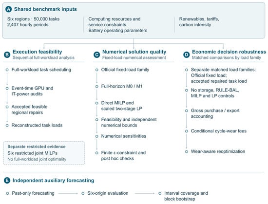
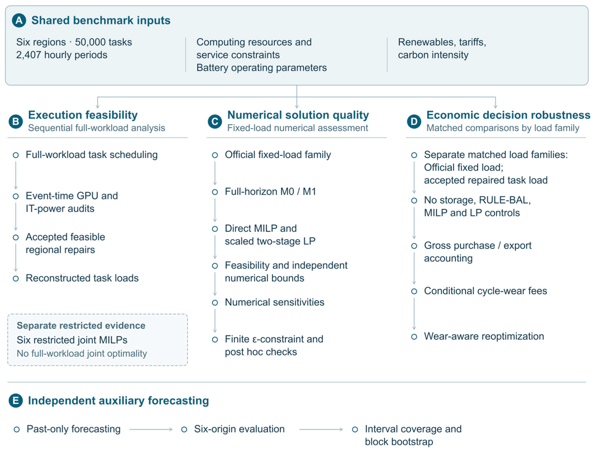
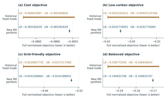
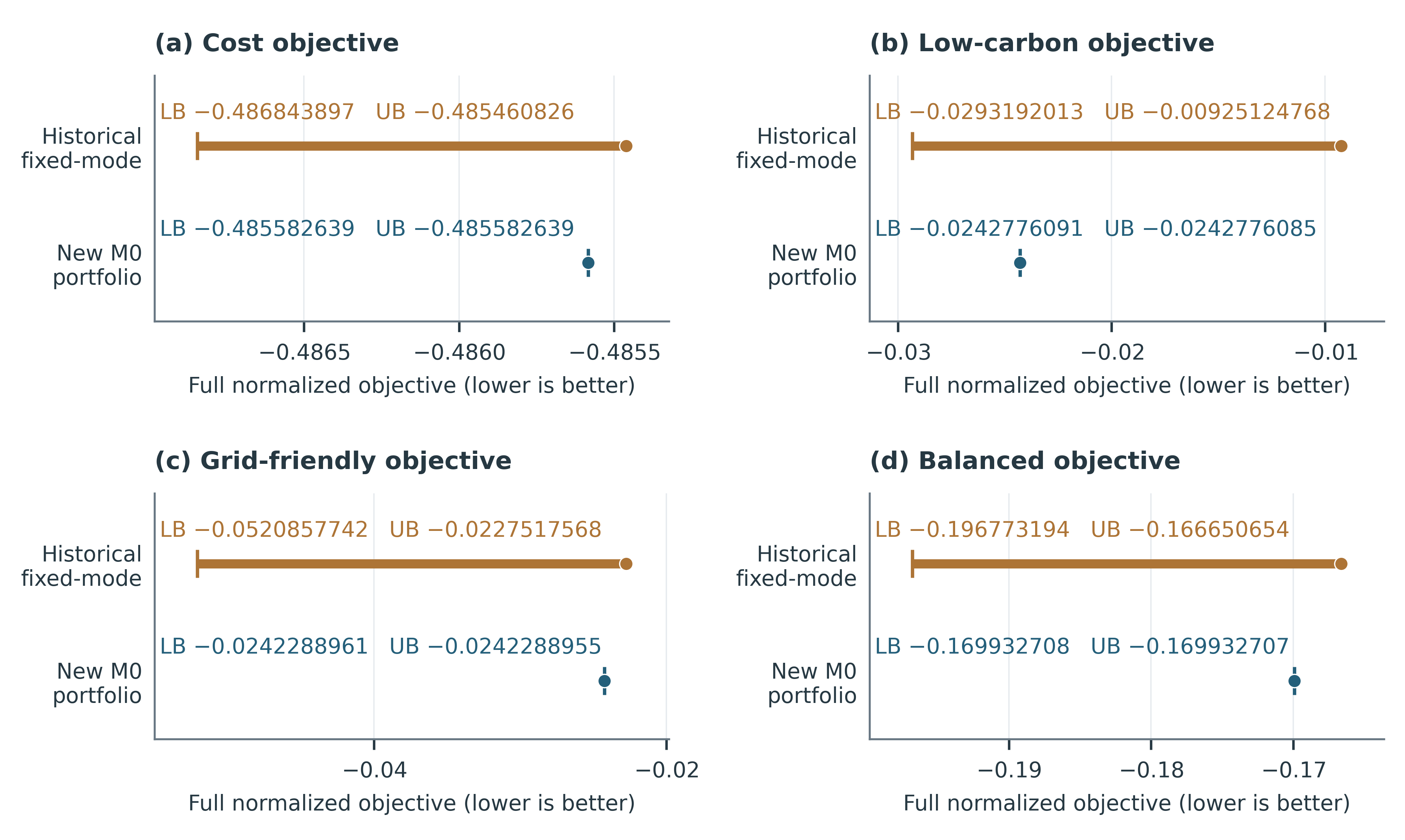
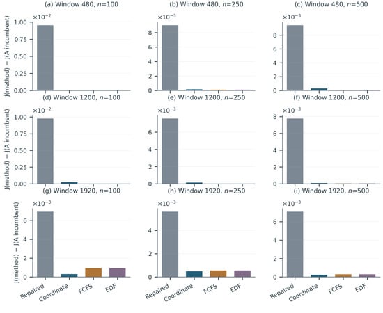
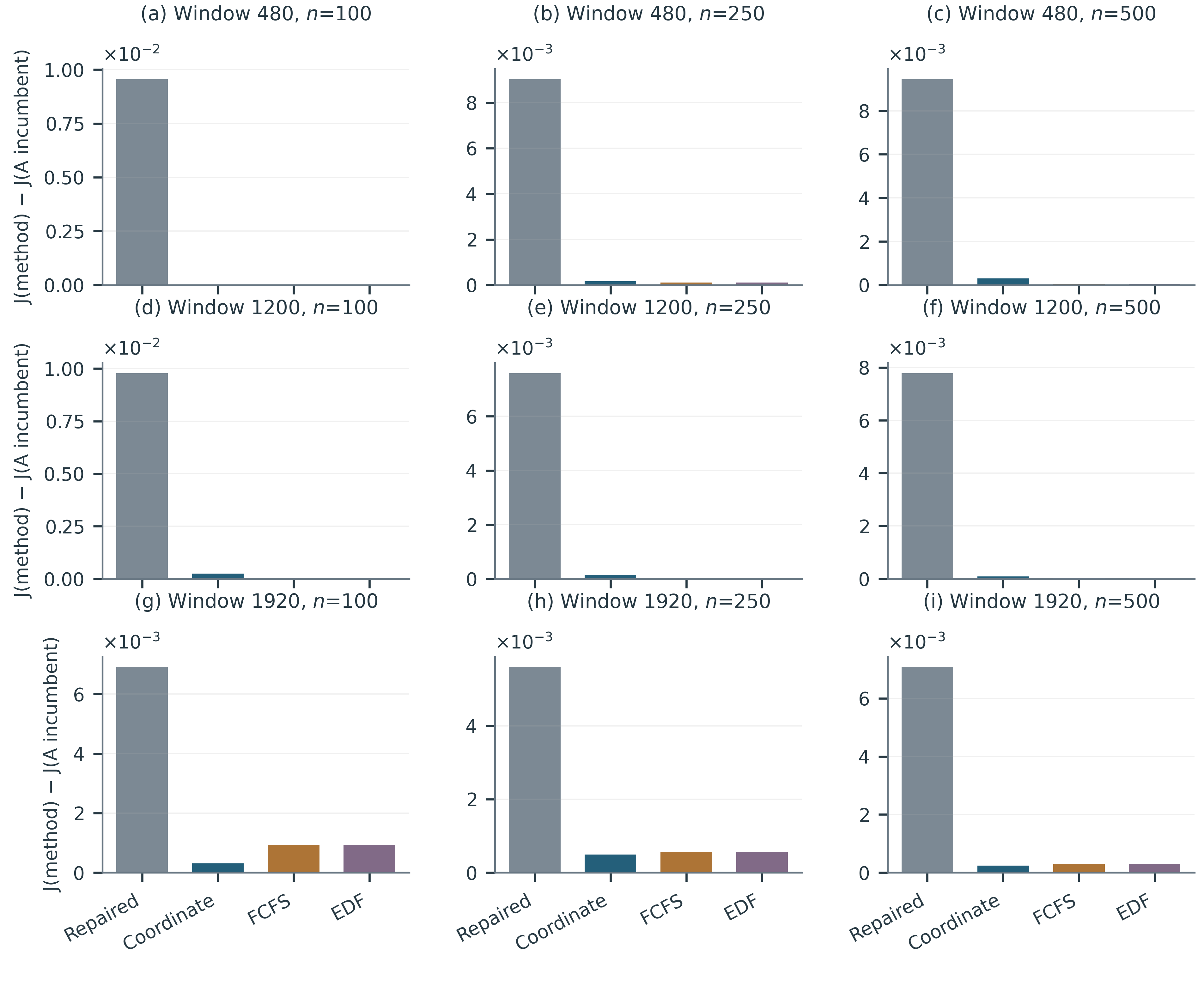
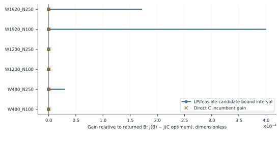
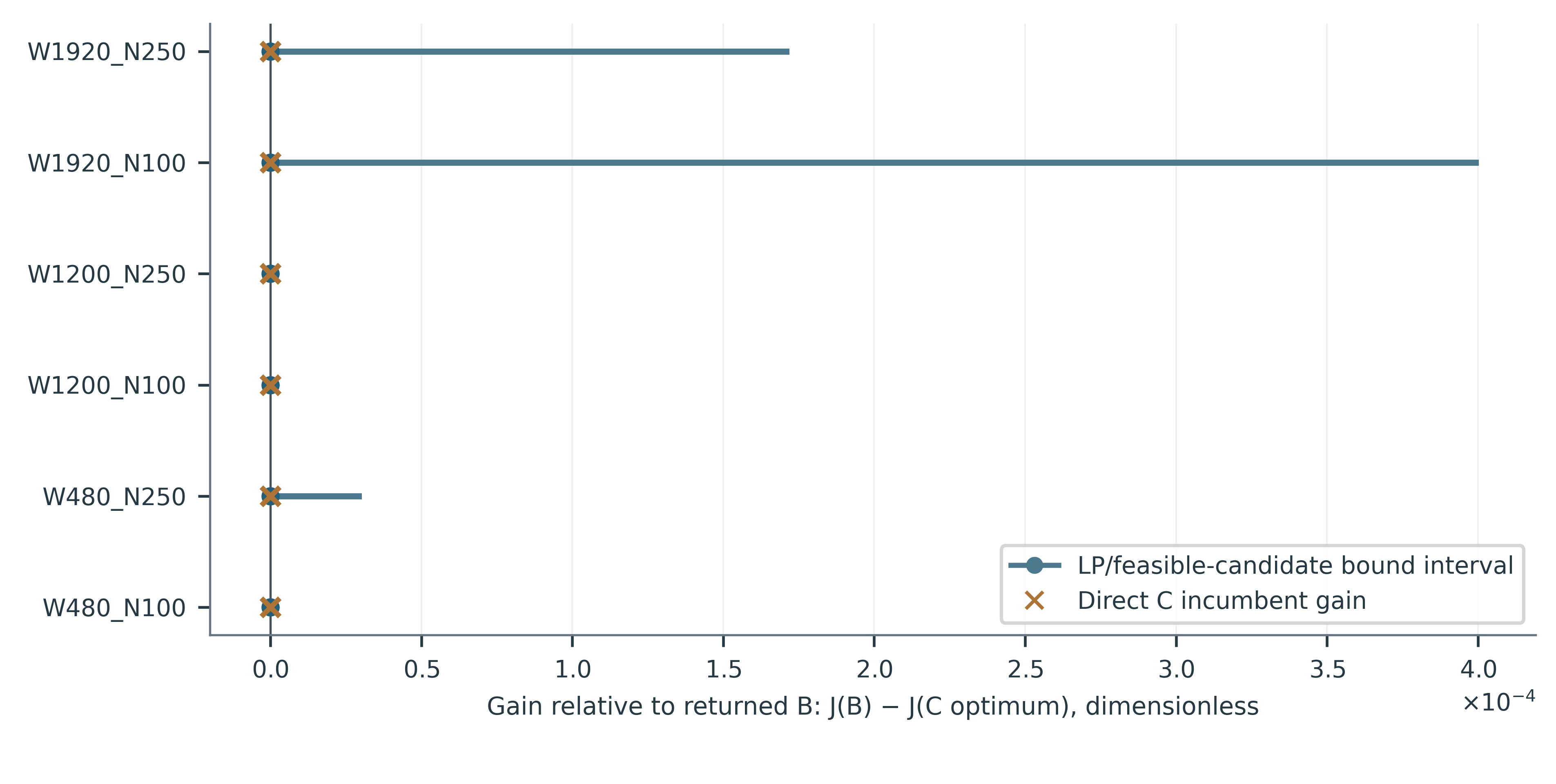
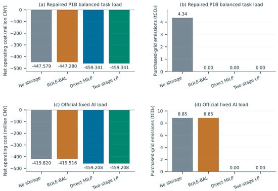
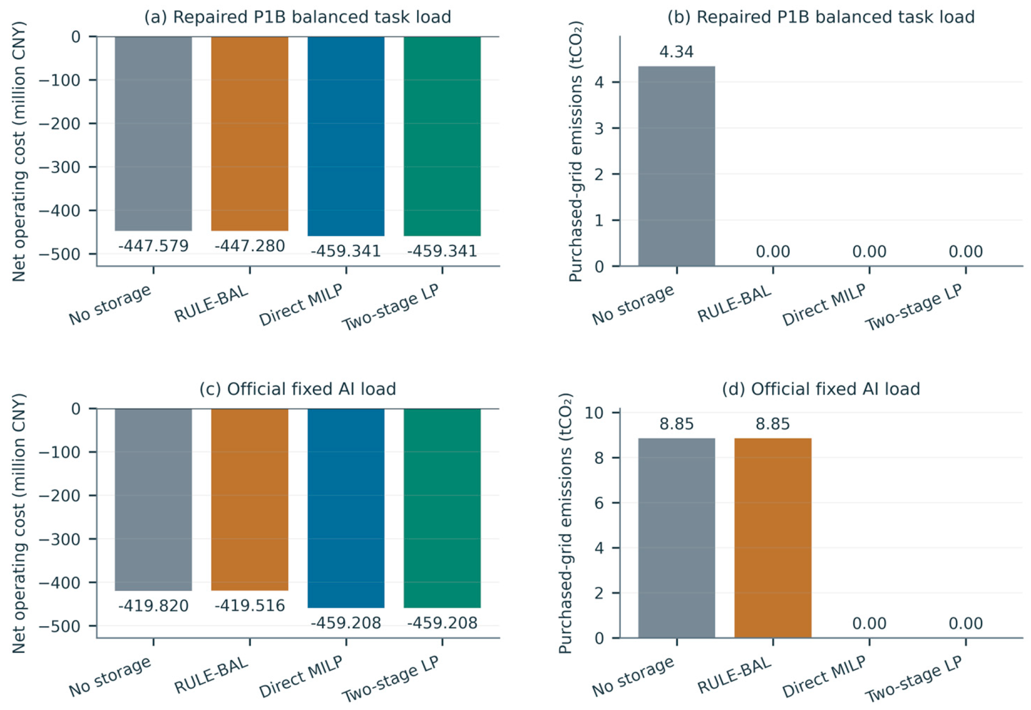
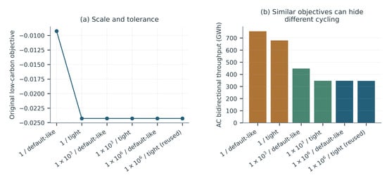
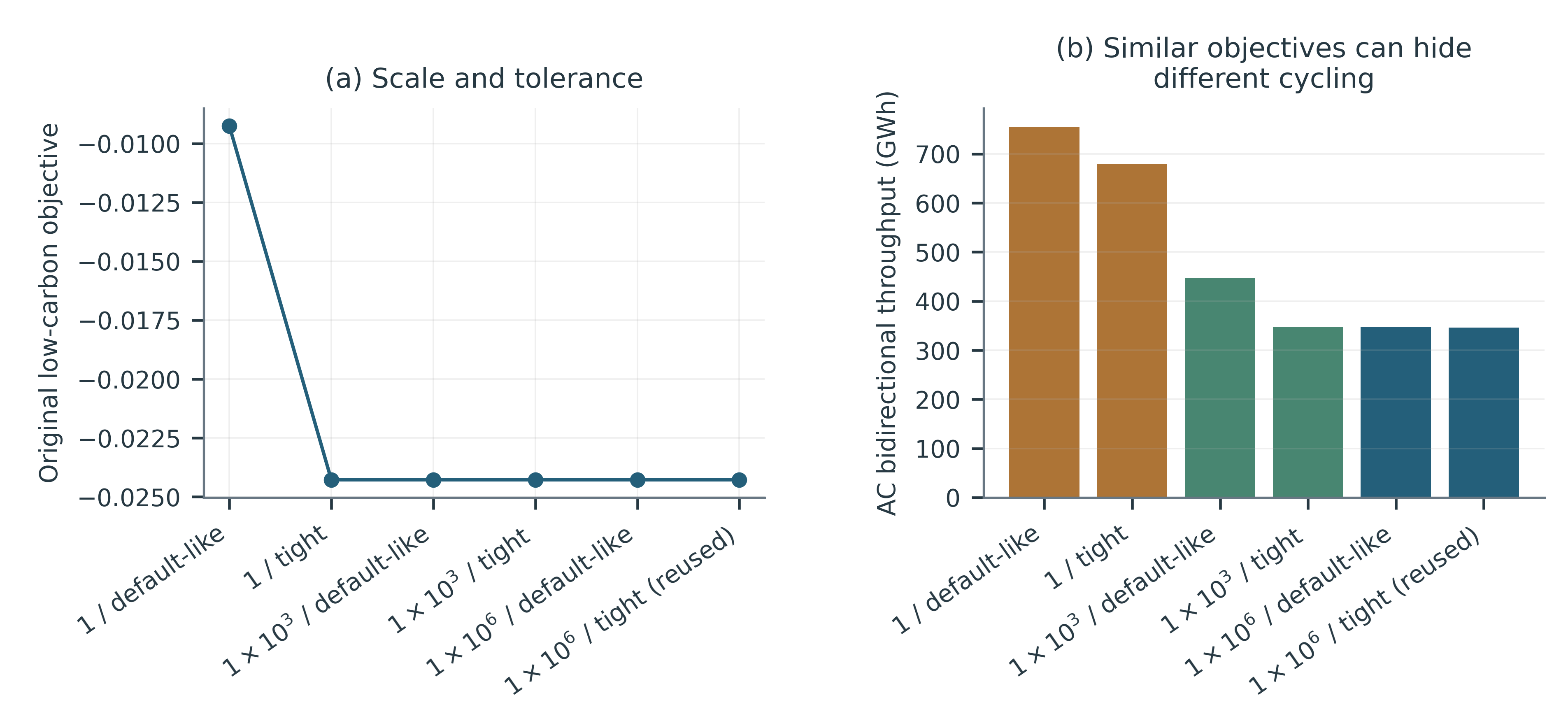
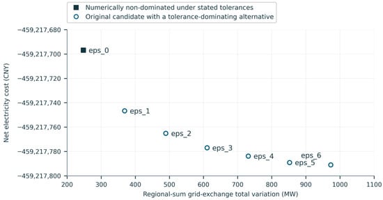
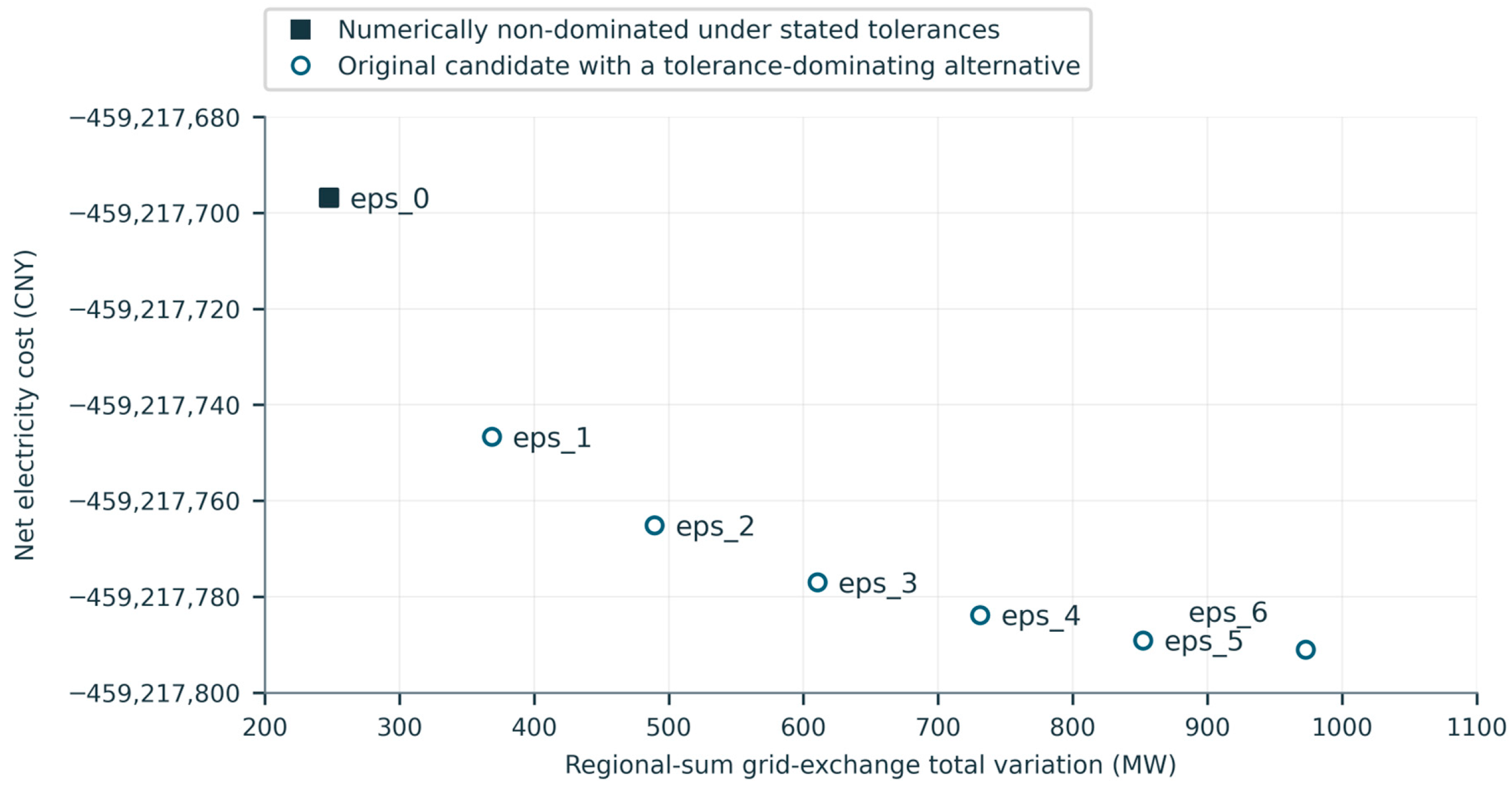

Disclaimer/Publisher’s Note: The statements, opinions and data contained in all publications are solely those of the individual author(s) and contributor(s) and not of MDPI and/or the editor(s). MDPI and/or the editor(s) disclaim responsibility for any injury to people or property resulting from any ideas, methods, instructions or products referred to in the content. |
© 2026 by the authors. Licensee MDPI, Basel, Switzerland. This article is an open access article distributed under the terms and conditions of the Creative Commons Attribution (CC BY) license.