Two-Timescale Frequency Control of Grid-Forming Energy Storage in Islanded Microgrids Based on Meteorological Warnings

Abstract

In islanded microgrids, a sudden drop in photovoltaic (PV) power causes severe frequency dips, whereas grid-forming energy storage relying on droop control alone exhibits a steady-state deviation that cannot be eliminated; increasing the damping coefficient converges only slowly and is constrained by the droop regulation ratio and the frequency deadband. To address this, this paper proposes a two-timescale frequency control method based on meteorological warnings. On the slow timescale, meteorological warnings are used to apply active-power feedforward against the PV drop caused by cloud passage, compressing the disturbance that droop must compensate from the entire power deficit to the prediction residual; on the fast timescale, virtual inertia and damping are pre-scheduled according to the bound of the prediction residual, raised before the disturbance and released afterwards. An input-to-state stability (ISS) theorem is established for the closed-loop system, proving that the frequency deviation is input-to-state stable with respect to the bounded prediction residual, from which the inertia/damping scheduling law and the feasible residual region are derived. Using a random forest predictor trained on three years of hourly measured meteorological data from a region in Hubei, together with a four-method benchmark and end-to-end ablation experiments, the results show that under an 85% PV drop the proposed method restores the steady-state frequency from 48.33 Hz to 50.00 Hz and reduces the maximum rate of change of frequency (RoCoF) in the fast transient from 0.81 Hz/s to 0.17 Hz/s with feedforward alone and to 0.06 Hz/s with the complete two-timescale controller; with a real event-level prediction error of 0.064, the steady-state compliance rate (not lower than 49.8 Hz) reaches 91.7% using the empirical event-level error distribution (94.4% under the Gaussian approximation), far above that of conventional droop control.

1. Introduction

Islanded microgrids lack the frequency support of a bulk power grid, and frequency regulation relies mainly on the inertia and damping provided by grid-forming energy storage (ESS) through virtual synchronous generator (VSG) control [1,2]. As PV penetration increases, short-term large-proportion output drops caused by cloud passage directly threaten frequency security [3,4,5], which makes the control performance of grid-forming ESS decisive for whether the system can operate stably.

Conventional droop control is a proportional control: the steady-state frequency deviation $\Delta f_{ss}={\displaystyle \frac{f_n\cdot \Delta P}{D+d_{load}}}$ cannot be eliminated, because a power response exists only when a frequency deviation is present. The only way to reduce the steady-state deviation is to increase the damping $D$, but this converges as $1/D$: at $D=20$ the steady-state frequency is merely $48.33 \mathrm{Hz}$, and it rises to $D$ only after $400$ is increased to $49.92 \mathrm{Hz}$; the cost of continuing to push the frequency toward its nominal value grows sharply, and doing so is infeasible in practice because it is bounded by the national standard on the primary frequency regulation droop ratio of energy storage [6,7] (about $0.5\sim 3\%$, corresponding to a damping coefficient of $33\sim 200$) and by the frequency deadband floor. On the other hand, the effects of inertia $H$ and damping $D$ on transient metrics conflict with each other: increasing $H$ lowers the rate of change of frequency (RoCoF) but slows the response and deepens the dip, whereas increasing $D$ reduces the dip but aggravates both the RoCoF and the steady-state deviation; fixed parameters can only compromise between the two [8,9,10,11].

Existing studies addressing the above issues broadly follow three lines. First, weather forecasting is introduced into the decisions on reserve and inertia provision: for example, Chang et al. [12,13] reserve regulation capacity according to the predicted curtailment of solar power. This is essentially reserve scheduling rather than power feedforward and does not change the steady-state structure of droop control. Second, the power deficit is inferred from the measured frequency: for instance, Ref. [14] employs a disturbance observer combined with offline model predictive control, which belongs to reactive compensation; the observer convergence delay is about $0.3 \mathrm{s}$, so frequency support is lost over that interval during fast transients. Third, the droop coefficient is adapted: for example, the frequency deviation is explicitly incorporated into the adjustment of the damping coefficient, but the scheme remains a proportional control and the steady-state deviation is retained as is.

A qualitative comparison of these routes is summarized in Section 4.4: none of them compensates the disturbance in the power domain using a weather forecast while simultaneously scheduling the fast-timescale inertia and damping, which is the gap addressed here.

To overcome these shortcomings, this paper proposes a two-timescale frequency control method based on meteorological warnings. The main contributions are as follows:

(1)

A slow/fast dual-timescale decomposition is proposed. On the slow timescale, meteorological warnings are exploited to apply active-power feedforward in the power domain against the predictable cloud-front drop, compressing the disturbance that droop must compensate from the entire power deficit to the prediction residual; on the fast timescale, adaptive inertia and damping scheduling is applied to the unpredictable prediction residual. The two are assigned distinct roles and neither encroaches on the other.

(2)

An input-to-state stability (ISS) theorem is established for the closed-loop system, proving that the frequency deviation is input-to-state stable with respect to the bounded prediction residual. The inertia/damping scheduling law and the feasible residual region are derived from it, constraining the RoCoF and the frequency dip within prescribed thresholds simultaneously.

(3)

The prediction error is calibrated on three years of hourly measured meteorological data from a region in Hubei, and a four-method benchmark comparison together with end-to-end ablation experiments verify the advantages of the proposed method over the three existing lines of work in both the steady state and the transient.

2. System Modeling and Problem Statement

2.1. System Structure and VSG Swing Equation

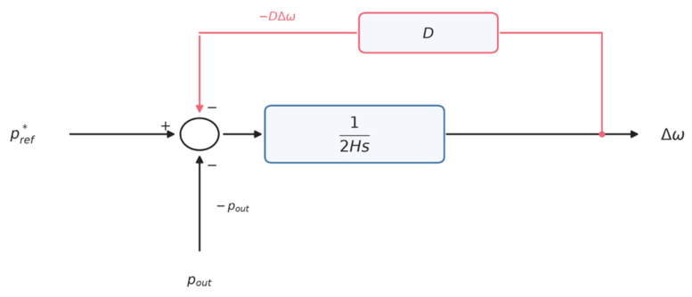
The object of study is an islanded microgrid comprising PV generation, load, grid-forming ESS (Figure 1), in which the grid-forming ESS is the sole voltage/frequency master source. The PV unit is interfaced through a grid-following inverter, which regulates its current and does not provide voltage or frequency support [15]; the grid-forming ESS therefore acts as the voltage/frequency master. Neglecting electromagnetic transients, the ESS adopts virtual synchronous generator (VSG) control (Figure 2), and its active-power-frequency dynamics are described by the per-unit swing equation:

Figure 1. Topology of the islanded microgrid. The PV unit is connected through a grid-following inverter [15], whereas the grid-forming ESS (5 MW/15 MWh) is the voltage/frequency master.

Figure 1. Topology of the islanded microgrid. The PV unit is connected through a grid-following inverter [15], whereas the grid-forming ESS (5 MW/15 MWh) is the voltage/frequency master.

$$2H{\displaystyle \frac{d\left(\Delta \omega \right)}{dt}}=p_{ref}-p_{net0}-\left(D+d_{load}\right)\Delta \omega$$

(1)

where $\Delta \omega =\omega -1$ is the per-unit angular frequency deviation; $H$ is the virtual inertia; $D$ is the active-power damping coefficient, which satisfies $\sigma$ together with the droop ratio $\sigma ={\displaystyle \frac{100}{D}}\%$; $d_{load}$, the equivalent damping of the frequency-dependent static aggregate load $P_L=P_{L0}(1+K_L\Delta f)$ with $K_L=1.5\%/\mathrm{Hz}$, is converted as $d_{load}={\displaystyle \frac{P_{load}}{S_B}}\cdot K_{load}\cdot f_n$= 0.375 for a 5 MW load; $p_{ref}$ is the ESS active-power reference and $p_{net0}={\displaystyle \frac{P_{load}-P_{PV}}{S_B}}$ is the net load excluding the frequency correction; all quantities are per unit. The base capacity is $S_B=10 \mathrm{MVA}$, the nominal frequency is $f_n=50 \mathrm{Hz}$, the PV rating is $P_{PV}^{rated}=8 \mathrm{MW}$. The ESS is rated 5 MW/15 MWh (3 h at nominal power). The converter is rated 5 MW continuously and is allowed a 1.2 p.u. short-time overload (6 MW), i.e., ±0.6 p.u. on the 10 MVA base; this is the ±6 MW envelope applied in all simulations. The ESS output is hard-limited to this envelope at every integration step.

Figure 2. Block diagram of VSG active-power/frequency control for grid-forming energy storage. The summing junction implements $2H\cdot {\displaystyle \frac{d\Delta \omega }{dt}} = P_{ref}\ast - P_{out} - D\cdot \Delta \omega$; that is, $P_{ref}\ast$ is added and $P_{out}$ is subtracted. Since the measured ESS output satisfies $P_{out}=P_{net0}+d_{load}\cdot \Delta \omega$, this is equivalent to Equation (1).

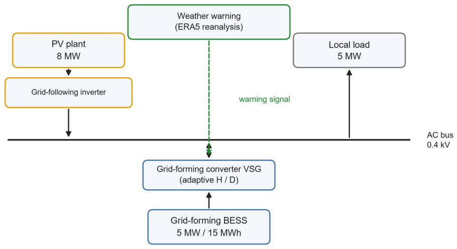
Figure 2. Block diagram of VSG active-power/frequency control for grid-forming energy storage. The summing junction implements $2H\cdot {\displaystyle \frac{d\Delta \omega }{dt}} = P_{ref}\ast - P_{out} - D\cdot \Delta \omega$; that is, $P_{ref}\ast$ is added and $P_{out}$ is subtracted. Since the measured ESS output satisfies $P_{out}=P_{net0}+d_{load}\cdot \Delta \omega$, this is equivalent to Equation (1).

Setting the left-hand side of Equation (1) to zero gives the steady-state solution:

$$\Delta f_{ss}={\displaystyle \frac{f_n\left(p_{ref}-p_{net0}\right)}{D+d_{load}}}$$

(2)

2.2. Structural Deviation of Droop Control

Conventional droop control keeps $p_{ref}=p_{ref0}$ unchanged ($p_{ref0}$ is the pre-disturbance net load). After a PV drop of $\Delta P$, we have $p_{ref}-p_{net0}=-\Delta P$, and from Equation (2):

$$\Delta f_{ss}=-{\displaystyle \frac{f_n\Delta P}{D+d_{load}}}$$

(3)

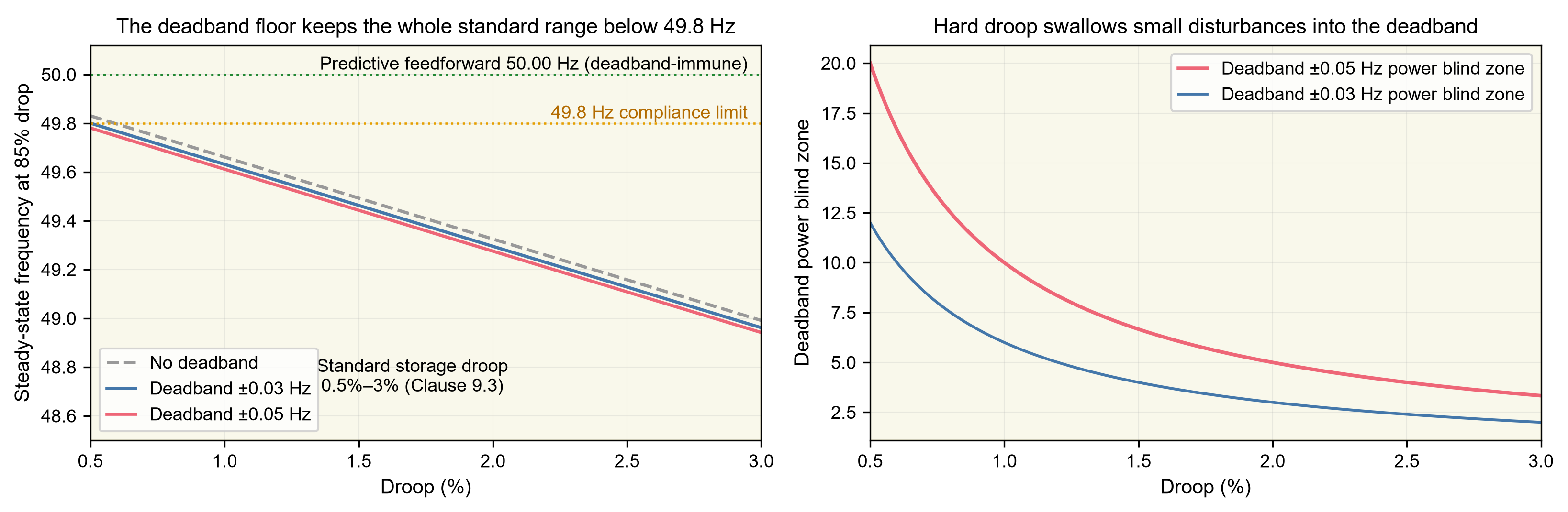
This shows that the steady-state frequency deviation is proportional to the deficit and inversely proportional to the damping, which is an inherent property of proportional control: a power response exists only when a frequency deviation is present. Taking a PV drop of $85\%$ ($\Delta P=0.68 \mathrm{p}.\mathrm{u}.$) with $D=20$ and $\Delta f_{ss}=-1.67 \mathrm{Hz}$, the steady-state frequency is merely $48.33 \mathrm{Hz}$. The deviation can be reduced only by increasing $D$, but this converges as $1/D$, and $D$ is constrained by the national standard on the droop ratio and by the frequency deadband, so this structural deviation cannot be eliminated (Figure 3).

Figure 3. Cost of the droop deadband.

Figure 3. Cost of the droop deadband.

2.3. Closed-Loop Dynamics After Feedforward Compensation and Problem Statement

This paper introduces active-power feedforward on the basis of Equation (1), such that:

$$p_{ref}=p_{ref0}+\mathrm{gain}\cdot {\hat{P}}_{drop}$$

(4)

where ${\hat{P}}_{drop}$ is the predicted amplitude of the PV drop provided by the meteorological warning ($\mathrm{p}.\mathrm{u}.$ of the PV rating), and $\mathrm{gain}={\displaystyle \frac{P_{PV}^{rated}}{S_B}}=0.8$ converts the amplitude quantity into a per-unit power quantity. Let the actual drop amplitude be $P_{drop}$; then the prediction residual is $\epsilon ={\hat{P}}_{drop}-P_{drop}$ ($\mathrm{p}.\mathrm{u}.$ of the PV rating), which converts into the power residual:

$$e=\mathrm{gain}\cdot \epsilon$$

(5)

Substituting into Equation (1), the closed-loop dynamics after feedforward compensation are:

$$2H{\displaystyle \frac{d\left(\Delta \omega \right)}{dt}}=-e-\left(D+d_{load}\right)\Delta \omega$$

(6)

Equation (6) shows that feedforward compresses the disturbance that droop must compensate from the entire deficit $\Delta P$ to the prediction residual $e$, and the steady-state frequency deviation becomes $\Delta f_{ss}={\displaystyle \frac{f_{n}e}{D+d_{load}}}$ accordingly. The frequency control problem thus reduces to two sub-objectives:

(i)

Steady-state sub-objective: compress the prediction residual $e$ so that $\Delta f_{ss}$ is as small as possible. This is accomplished by the slow-timescale feedforward, and under a perfect warning ($e=0$) the steady state is exactly $50.00 \mathrm{Hz}$.

(ii)

Transient sub-objective: for the residual $e$ that cannot be eliminated, constrain the initial $\mathrm{RoCoF}={\displaystyle \frac{f_{n}e}{2H}}$ and the frequency dip ${\displaystyle \frac{f_{n}e}{D+d_{load}}}$ below prescribed thresholds. This is accomplished by the fast-timescale adaptive $H/D$.

2.4. Model and Notation

Justification of the single-machine model: in an islanded microgrid the electrical distances are short and the frequency is globally uniform within a few seconds (a single coherent area); the voltage/reactive-power loop is quasi-static, slower than, and therefore decoupled from, the active-power-frequency loop. This paper focuses on the frequency (active-power) subsystem driven by meteorological disturbances, for which the single-machine swing Equation (1) is a standard and sufficient abstraction; a later extension to multiple machines will not affect the method or the conclusions of this paper.

Unit conventions (used throughout to avoid confusion between amplitude and power): $\epsilon$ and ${\sigma }_{\epsilon }$ are amplitude errors ($\mathrm{p}.\mathrm{u}.$ of the PV rating, $8 \mathrm{MW}$); $e$ is the power residual ($\mathrm{p}.\mathrm{u}.$ of the base capacity, $10 \mathrm{MW}$); the two are bridged by $\mathrm{gain}=0.8$; the frequency deviation is computed from ${\displaystyle \frac{f_{n}e}{D+d_{load}}}$. All prediction errors ${\sigma }_{\epsilon }$ reported in this paper refer to the amplitude convention and are uniformly multiplied by $\mathrm{gain}$ to convert them into power residuals before being substituted into the scheduling law. In particular, all residual thresholds reported in this paper (for example, the feasible residual bound $e_{feas}=0.0815 \mathrm{p}.\mathrm{u}.$) refer to the power-residual convention $e$, whereas the prediction-accuracy requirement ${\sigma }_{\epsilon }\le 0.10 \mathrm{p}.\mathrm{u}.$ refers to the amplitude convention; the two are related by $e=\mathrm{gain}·{\sigma }_{\epsilon }$.

The main symbols are listed in Table 1.

Table 1. Main symbols.

Symbol	Meaning	Value
$S_B/f_n$	Base capacity/nominal frequency	$10 \mathrm{MVA}/50 \mathrm{Hz}$
$P_{PVrated}$	PV rating	8 MW
$P_{ESSnom}$	ESS continuous rating (energy)	5 MW (15 MWh)
$P_{ESSmax}$	ESS transient overload (1.2 p.u.)	6 MW
$H$	Virtual inertia	$0.5\sim 6 \mathrm{s}$ (base value $2$)
$D$	Active-power damping (droop ratio $100/D\%$)	$0.5\sim 20$ (base value $1.5$)
$d_{load}$	Converted load self-regulation damping	$0.375$
$\mathrm{gain}$	Amplitude $\to$ to power conversion coefficient $P_{PV}^{rated}/S_B$	$0.8$
$\epsilon /{\sigma }_{\epsilon }$	Amplitude prediction error/its standard deviation	-
$e$	Power residual $=\mathrm{gain}\cdot \epsilon$	-
$R_{lim}/\Delta f_{lim}$	RoCoF limit/frequency dip limit	$0.5 \mathrm{Hz}/\mathrm{s}/0.2 \mathrm{Hz}$

3. Two-Timescale Adaptive Control Method

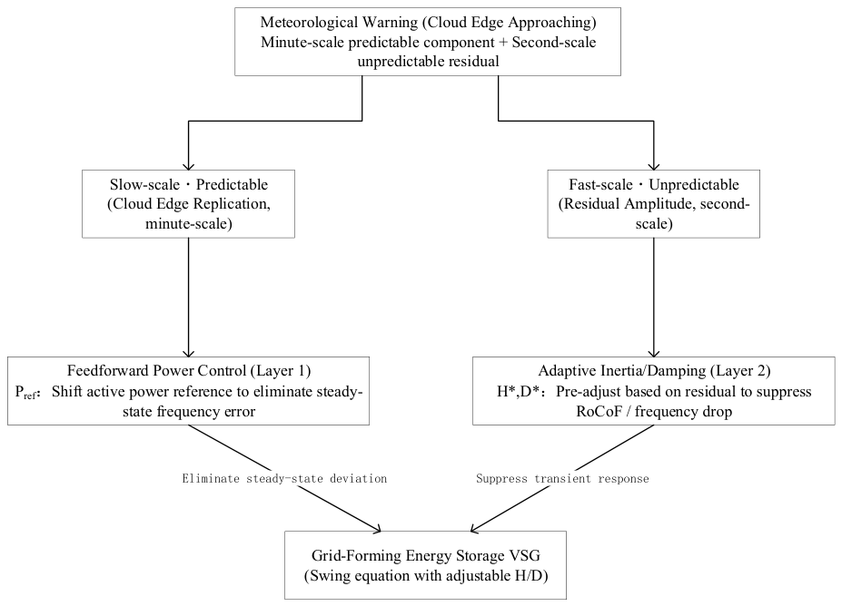
This section presents the complete structure of the proposed method (Figure 4). The overall idea is to decompose the frequency regulation problem of the islanded microgrid into two timescales according to the temporal characteristics of the disturbance: the PV power drop caused by cloud passage is a slow process that can be forecast in advance and compensated by feedforward at the power level, whereas the forecast error manifests itself as an unpredictable fast process whose transient impact must be suppressed by the real-time adjustment of inertia and damping. The two act respectively on two groups of control degrees of freedom in the closed-loop Equation (6), namely the active-power reference $p_{ref}$ and the inertia $H$ and damping $D$, with the former determining the steady state and the latter the transient; their roles are clearly separated and neither encroaches on the other.

Figure 4. Overall architecture of the two-timescale adaptive control.

Figure 4. Overall architecture of the two-timescale adaptive control.

3.1. Slow Timescale: Active-Power Feedforward from Meteorological Warnings

The value of a meteorological warning lies in providing a prediction of both the amplitude and the arrival time of the PV drop before the disturbance actually occurs [16,17,18,19]. If the ESS can be made to increase its active-power output by the same amount at the very instant the drop occurs, then the droop loop in principle no longer needs to respond to the frequency deviation, and the steady-state deviation is eliminated. To this end, the feedforward shifts the active-power reference as follows:

$$p_{ref}^{\ast }=p_{ref0}+\mathrm{gain}\cdot {\hat{P}}_{drop}$$

(7)

where ${\hat{P}}_{drop}$ is the predicted drop amplitude given by the warning ($\mathrm{p}.\mathrm{u}.$ of the PV rating) and $\mathrm{gain}={\displaystyle \frac{P_{PV}^{rated}}{S_B}}=0.8$ converts it into a per-unit power; $p_{ref0}$ is the pre-disturbance net load. Considering the ramp-rate limit of the ESS converter, the actual reference follows:

$$p_{ref}\left(t\right)=p_{ref}\left(t-\Delta t\right)+\mathrm{clip}\left(p_{ref}^{\ast }-p_{ref}\left(t-\Delta t\right),\pm \rho \cdot \Delta t\right)$$

(8)

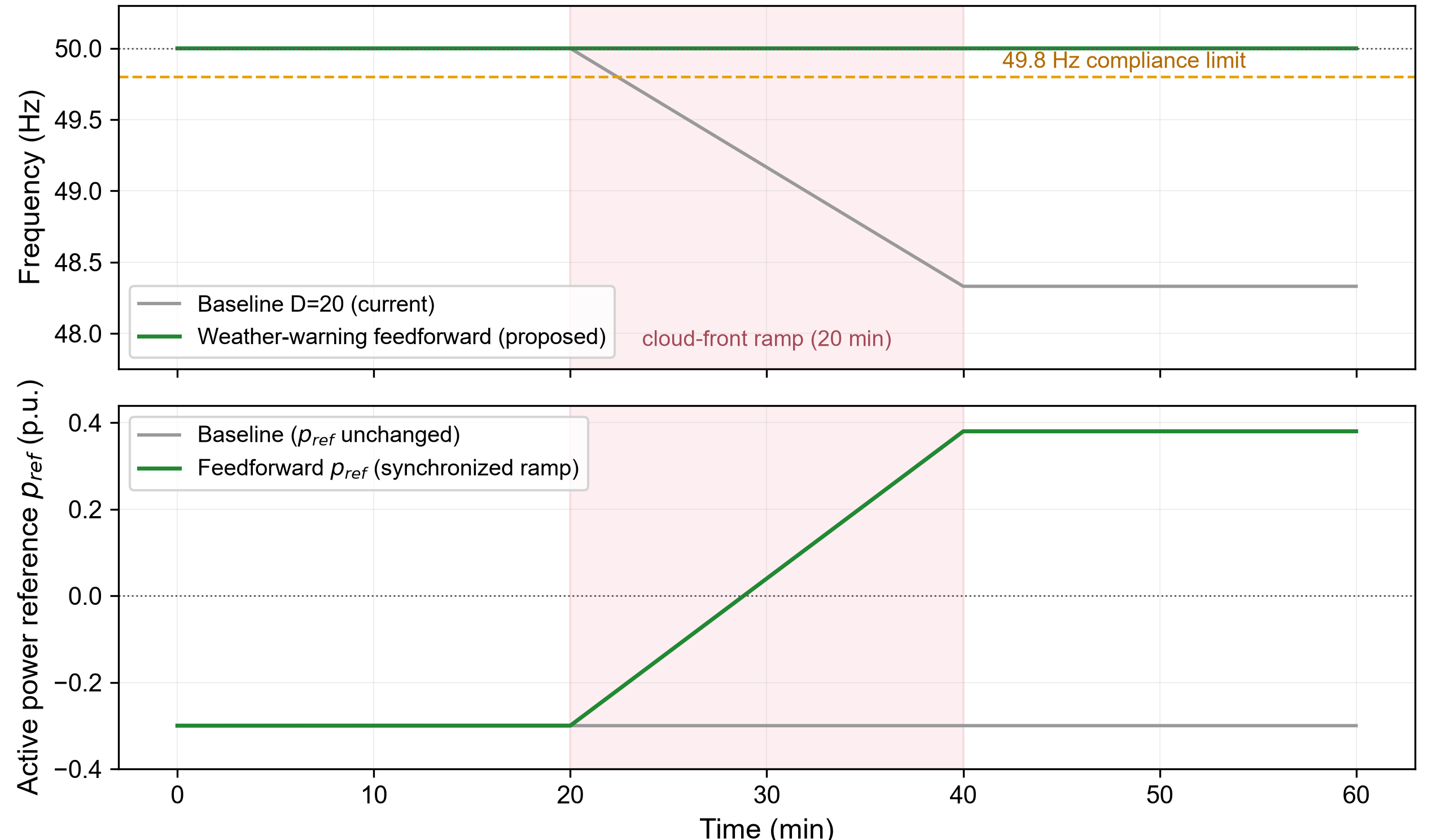
which approaches the target gradually (Figure 5), where $\rho$ is the admissible ramp rate (taken as $0.34 \mathrm{p}.\mathrm{u}./\mathrm{s}$ in this paper). Meanwhile, in order to avoid an advance shift caused by a mismatch between the predicted and the actual instants of the drop, ${\hat{P}}_{drop}$ in Equation (7) is taken as the running peak of the predicted drop amplitude within the warning window, and it takes effect after a delay of ${\mathrm{delay}}_s$ (set equal to the look-ahead time of the warning), so that the feedforward starts synchronously with the drop (Figure 6).

Figure 5. Internal structure of the feedforward controller.

Figure 5. Internal structure of the feedforward controller.

The physical effect of the feedforward can be seen directly from Equations (5) and (6): it compresses the disturbance actually faced by the droop loop from the entire deficit $\Delta P$ to the prediction residual $e=\mathrm{gain}\cdot \epsilon$. When the prediction is unbiased and accurate ($\epsilon =0$), only the damping term remains on the right-hand side of Equation (6), the steady-state frequency is exactly $50.00 \mathrm{Hz}$, and the structural deviation inherent in droop control is completely eliminated. In addition, the feedforward has three important properties. First, it shifts $p_{ref}$ directly in the power domain without passing through the frequency deadband, and is therefore immune to the droop deadband, an advantage that is difficult to obtain in the frequency domain. Second, it introduces no integral action on the frequency error; the droop loop is retained as is and the system remains a droop regulator with non-zero steady-state error. Feedforward only changes the amount of disturbance that must be covered by droop, and does not alter the regulation structure itself. Third, as Equation (2) shows, the steady-state solution depends only on the power balance and is independent of the time constants and of the disturbance timescale; therefore, whether the disturbance is a $2 \mathrm{s}$ step drop or a $20 \min$ ramp, the steady-state improvement brought by the feedforward is exactly the same, and the method is inherently robust to the disturbance timescale.

Figure 6. Slow-timescale cloud-front feedforward.The shaded band marks the 20-min cloud-front ramp period, and the dashed line is the 49.8 Hz compliance limit.

Figure 6. Slow-timescale cloud-front feedforward.The shaded band marks the 20-min cloud-front ramp period, and the dashed line is the 49.8 Hz compliance limit.

3.2. Fast Timescale: Predictive Adaptive Inertia/Damping

Feedforward eliminates the steady-state deviation, but it cannot guarantee an absolutely accurate prediction. The residual $e$ still excites the frequency transient through Equation (6), which manifests itself as two quantities: the initial RoCoF and the steady-state dip. The idea of this paper is that, since the statistical upper bound of the residual $\overline{e}$ can be estimated in advance from the prediction error, the inertia $H$ and damping $D$ can also be raised before the disturbance arrives, so as to suppress the residual-driven transient with the tightest possible parameters. Let the residual satisfy $|e|\le \overline{e}$; the scheduling law is then:

$$H^{\ast }=\mathrm{clamp}\left({\displaystyle \frac{f_n\overline{e}}{2R_{lim}}},H_{min},H_{max}\right)$$

(9)

$$D^{\ast }=\mathrm{clamp}\left({\displaystyle \frac{f_n\overline{e}}{\Delta f_{lim}}}-d_{load},D_{min},D_{max}\right)$$

(10)

$$H=\max \left(H_{base},H^{\ast }\right),D=\max \left(D_{base},D^{\ast }\right)$$

(11)

where $R_{lim}$ and $\Delta f_{lim}$ are the upper limits on the RoCoF and on the frequency dip, respectively. When the warning is triggered (the predicted drop exceeds the threshold), $H$ and $D$ are raised in advance according to Equations (9)–(11); after the disturbance ends they fall back to the base values $H_{base}$ and $D_{base}$ so as to accelerate recovery. The residual bound $\overline{e}$ is constructed from the prediction error as:

$$\overline{e}=\mathrm{gain}\cdot k_{\sigma }\cdot {\sigma }_{\epsilon }$$

(12)

${\sigma }_{\epsilon }$ is the standard deviation of the drop-amplitude prediction error ($\mathrm{p}.\mathrm{u}.$ of the PV rating), and $k_{\sigma }$ is the confidence coefficient ($1$ corresponds to the $1\sigma$ bound and $3$ to the $99.7\%$ hard bound; their conservativeness is discussed later). It should be emphasized that Equations (9)–(11) are not empirical tuning, but analytical solutions obtained by inverting the two classes of constraints from the stability result below, which is the key feature that distinguishes the proposed method from the empirical adaptive tuning in Ref. [20].

3.3. Stability Analysis and Parameter Design

After feedforward compensation, the closed-loop system is given by Equation (6). The following result characterizes the robustness of the frequency deviation with respect to the prediction residual and directly provides the design basis for the scheduling law in Equations (9)–(11).

Proposition 1.

For Equation (6), if the prediction residual satisfies $|e\left(t\right)|\le \overline{e}$, then the frequency deviation satisfies:

$$|\Delta f\left(t\right)|\le |\Delta f\left(0\right)|e^{-t/\tau }+{\displaystyle \frac{f_n\overline{e}\left(1-e^{-t/\tau }\right)}{D+d_{load}}}$$

(13)

where $\tau ={\displaystyle \frac{2H}{D+d_{load}}}$.

Proof. 

Let $V=H\cdot {\Delta \omega }^2$. Along (6), with $|e(t)|\le ē$,

$$2H\cdot \Delta \omega \cdot {\displaystyle \frac{d\Delta \omega }{dt}}=\Delta \omega [-e-(D+d_{load})\Delta \omega ]\le ē|\Delta \omega |-(D+d_{load}){\Delta \omega }^2$$

Using $ē|\Delta \omega |\le {\displaystyle \frac{(D+d_{load}){\Delta \omega }^2}{2}}+{\displaystyle \frac{{ē}^2}{2(D+d_{load})}}$, we obtain

$$\le -{\displaystyle \frac{(D+d_{load})}{2H}}\cdot V+{\displaystyle \frac{{ē}^2}{2(D+d_{load})}}$$

By the comparison lemma,

$$|\Delta \omega (t)|\le |\Delta \omega (0)|e^{{\displaystyle \frac{-t}{\tau }}}+{\displaystyle \frac{ē}{(D+d_{load})}},\tau ={\displaystyle \frac{2H}{(D+d_{load})}}$$

For the adaptive schedule, $H\in [0.5, 6] \mathrm{s} \mathrm{and} D\in [0.5, 20]$ are bounded, and the same V is a common Lyapunov function for every admissible (H, D); hence the bound holds uniformly with $D=D_{min} \mathrm{and} \tau ={\displaystyle \frac{2H_{max}}{(D_{min}+d_{load})}}$. □

Equation (13) shows that, no matter how the residual $e\left(t\right)$ varies with time within $\left[-\overline{e},\overline{e}\right]$, the frequency deviation always remains within the envelope given by Equation (13) and converges with the time constant $\tau$ to the ultimate bound ${\displaystyle \frac{f_n\overline{e}}{D+d_{load}}}$; this ultimate bound and the convergence rate ${\displaystyle \frac{D+d_{load}}{2H}}$ are determined solely by $\overline{e}$, $H$, and $D$. For the zero-initial-value case, taking the slope of the right-hand side of Equation (13) at $t\to 0^{+}$ and its limit as $t\to \infty$ yields the upper bounds on the initial RoCoF and on the steady-state dip, respectively:

$$\mathrm{Initial} \mathrm{RoCoF}={\displaystyle \frac{f_n\overline{e}}{2H}}\le R_{lim}⟹H\ge {\displaystyle \frac{f_n\overline{e}}{2R_{lim}}}$$

(14)

$$⟹D\ge {\displaystyle \frac{f_n\overline{e}}{\Delta f_{lim}}}-d_{load}$$

(15)

Equations (14) and (15) agree term by term with the scheduling law in Equations (9) and (10), which indicates that Equations (9)–(11) are exactly the tightest solution that places $H$ and $D$ precisely on the boundaries of the two classes of constraints, rather than an empirical tuning: the smallest parameters that guarantee simultaneous compliance of the RoCoF and the dip are selected, balancing transient suppression against response speed.

Furthermore, the two classes of constraints must be satisfied simultaneously, while $H$ and $D$ are themselves limited by their upper bounds $H_{max}$ and $D_{max}$; hence the largest residual bound that adaptive $H/D$ can suppress on its own is:

$${\overline{e}}_{feas}=\min \left({\displaystyle \frac{2H_{max}{R}_{lim}}{f_n}},{\displaystyle \frac{\left(D_{max}+d_{load}\right)\Delta f_{lim}}{f_n}}\right)$$

(16)

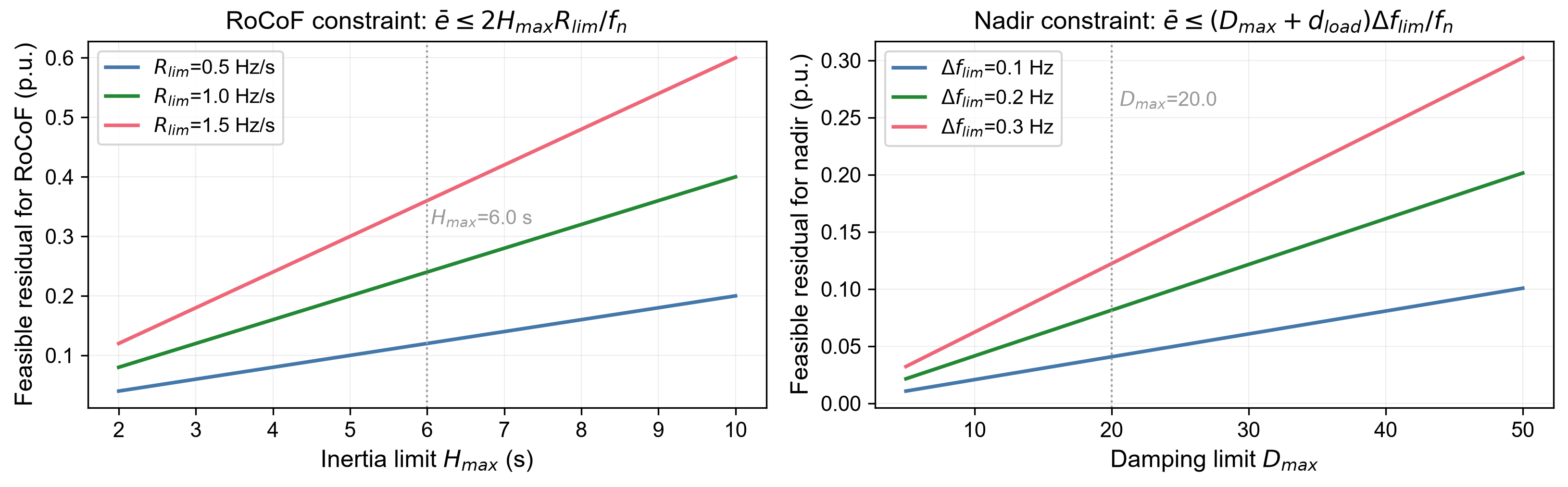
Substituting $H_{max}=6 \mathrm{s}$, $D_{max}=20$, $R_{lim}=0.5 \mathrm{Hz}/\mathrm{s}$, $\Delta f_{lim}=0.2 \mathrm{Hz}$, and $f_n=50 \mathrm{Hz}$ gives ${\overline{e}}_{feas}=\min \left(0.120, 0.0815\right)=0.0815 \mathrm{p}.\mathrm{u}.$, which means that the frequency-dip constraint binds before the RoCoF constraint. Inverting Equation (12), this is equivalent to requiring a prediction accuracy of ${\sigma }_{\epsilon }\le {\displaystyle \frac{{\overline{e}}_{feas}}{\mathrm{gain}\cdot k_{\sigma }}}=0.102$ (in the $1\sigma$ convention). Equation (16) thus delineates the division of labor between the two control layers: when the prediction residual lies within the base value $8.15\%$, adaptive $H/D$ alone can guarantee simultaneous compliance with both constraints; once the residual exceeds this bound, adaptive $H/D$ can no longer satisfy both constraints and the slow-timescale feedforward must compress the residual back into the feasible region. This is the fundamental reason why a joint two-timescale control is necessary, rather than relying on adaptive inertia/damping alone (Figure 7).

Figure 7. Feasible residual region.

Figure 7. Feasible residual region.

4. Validation

4.1. Simulation Setup and Evaluation Metrics

Simulations are carried out on the per-unit VSG swing Equation (6), with base capacity $S_B=10 \mathrm{MVA}$, nominal frequency $f_n=50 \mathrm{Hz}$, PV rating $8 \mathrm{MW}$, ESS rating $5 \mathrm{MW}$, load $5 \mathrm{MW}$, and load frequency sensitivity coefficient $1.5\%/\mathrm{Hz}$. The disturbance is set as a PV output drop of $85\%$ (that is, $8\to 1.2 \mathrm{MW}$, a deficit of $0.68 \mathrm{p}.\mathrm{u}.$), and two representative timescales are examined: a $2 \mathrm{s}$ step drop (approximating fast cloud shading) and a $450 \mathrm{s}$ ramp (slow passage of a cloud front). Except in Section 4.3, the feedforward uses the full warning amplitude with a look-ahead of $5 \mathrm{s}$ and a ramp-rate limit of $0.34 \mathrm{p}.\mathrm{u}./\mathrm{s}$. Four evaluation metrics are adopted: the steady-state frequency, the frequency nadir, the maximum RoCoF (${|\mathrm{RoCoF}|}_{max}$), and the minimum ESS state of charge (SOC); the steady-state value is taken as the mean over the last $40 \mathrm{s}$, and compliance is defined as a frequency not lower than $49.8 \mathrm{Hz}$. The simulation platform is Python 3.11, with a physical sub-step of $10 \mathrm{ms}$ and a control step of $100 \mathrm{ms}$.

4.2. Verification of the Stability Result

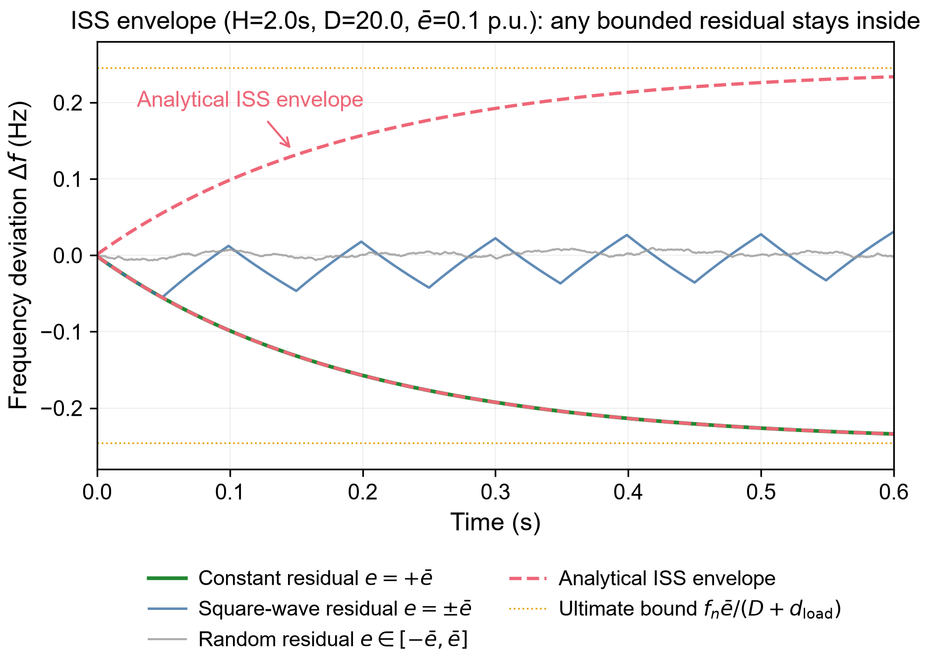
To verify the analytical accuracy of Proposition 1, we take $H=2 \mathrm{s}$, $D=20$, and a constant residual $e=0.10 \mathrm{p}.\mathrm{u}.$; Equation (13) gives the analytical time constant $\tau =0.1963 \mathrm{s}$ and steady-state frequency deviation $\Delta f_{ss}=-0.2454 \mathrm{Hz}$. The relative errors measured in simulation are $0.16\%$ and $1.06\%$, respectively, indicating that both the ultimate bound and the convergence rate of Equation (13) are exact rather than conservative estimates. Furthermore, letting the residual vary in time within $\left[-\overline{e},\overline{e}\right]$ in two ways, namely a square wave and a uniformly random signal, the simulated frequency deviation never crosses the envelope given by Equation (13) (Figure 8), which verifies the applicability of the input-to-state stability result to bounded time-varying residuals.

Figure 8. ISS stability envelope

Figure 8. ISS stability envelope

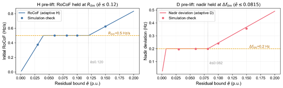
On this basis, the scheduling law in Equations (9)–(11) is re-examined: when the residual bound is $\overline{e}\le 0.0815 \mathrm{p}.\mathrm{u}.$, taking $H$ and $D$ according to Equations (9) and (10) makes the initial $\mathrm{RoCoF}\le 0.5 \mathrm{Hz}/\mathrm{s}$ and the frequency dip $\le 0.2 \mathrm{Hz}$ hold simultaneously; when $\overline{e}$ increases to $0.10$ and $0.15 \mathrm{p}.\mathrm{u}.$, $D$ saturates at $D_{max}=20$ and the frequency dip correspondingly exceeds $0.2 \mathrm{Hz}$, which is exactly consistent with the feasible residual bound ${\overline{e}}_{feas}=0.0815 \mathrm{p}.\mathrm{u}.$ given by Equation (16). This shows that the range over which adaptive $H/D$ satisfies the constraints is indeed determined by Equation (16), and that residuals beyond this range must be compressed by feedforward (Figure 9).

Figure 9. Constraint satisfaction of the adaptive inertia and damping (H/D).

Figure 9. Constraint satisfaction of the adaptive inertia and damping (H/D).

4.3. Calibration of the Prediction Error on Real Data

The prediction error ${\sigma }_{\epsilon }$ is the key parameter determining the performance of the method. In this paper, a random forest (RF) predictor [21,22] is trained on three years of hourly measured meteorological data from a region in Hubei (shortwave radiation, cloud cover, rate of change of cloud cover, rate of change of shortwave radiation, precipitation, and temperature), with the target being the PV drop amplitude in the next hour. The data are split chronologically (training/validation/testing = $2/3:1/6:1/6$), and only daytime samples are retained to avoid temporal leakage. The results are shown in Table 2: the F1 score of RF reaches $0.617$, a significant improvement over the $0.430$ of the persistence baseline, indicating that the meteorological features provide genuinely learnable warning information (Figure 10).

Table 2. Predictor performance and prediction error on real hourly data.

Metric	Persistence Baseline	Random Forest	95% CI (Bootstrap)
▪ F1	$0.430$	$0.617$	[0.570, 0.662]
$R^2$	$-0.094$	$0.468$	—
▪ $\mathrm{Overall} \mathrm{RMSE} {\sigma }_{\epsilon }$	$0.077$	$0.053$	—
▪ Number of events	$302$	$302$	—
▪ Event-level conditional RMSE	$0.132$	$0.084$	[0.0755, 0.0932]
▪ Event-level conditional bias	$-0.086$	$-0.055$	—
▪ $\mathrm{Event}\text{-}\mathrm{level} \mathrm{conditional} {\sigma }_{\epsilon }$	$0.100$	$0.064$	—

Bootstrap confidence intervals (10,000 resamples) are reported in Table 2. The paired difference in F1 is +0.187 (95% CI 0.141–0.234) with P(ΔF1 > 0) = 100%, confirming that the improvement over the persistence baseline is statistically significant (Figure 11).

Convention of the prediction error: the overall RMSE ($0.053$) is diluted by the large number of stationary periods with near-zero drops and does not represent the error magnitude actually faced by the controller. Analyzing separately the ≥15% event samples whose actual drop is $302$ of the rating, the conditional RMSE of RF is $0.084$ and the conditional standard deviation is ${\sigma }_{\epsilon }=0.064$, with a systematic underestimation of $-0.055$. Therefore, this paper adopts the event-level ${\sigma }_{\epsilon }=0.064$ as the real prediction error in the control simulations, and additionally takes ${\sigma }_{\epsilon }=0.151$ (a synthetic upper bound on the scale, also comparable to the $10\sim 20\%$ RMSE of intra-day and day-ahead PV forecasting reported in the literature) as a conservative bound; the sensitivity analysis covers the $0.06\sim 0.20$ range to ensure that the conclusions are insensitive to the error convention.

Figure 10. Warning prediction on real data and feature importance.

Figure 10. Warning prediction on real data and feature importance.

Figure 11. Baseline comparison of warning classification.

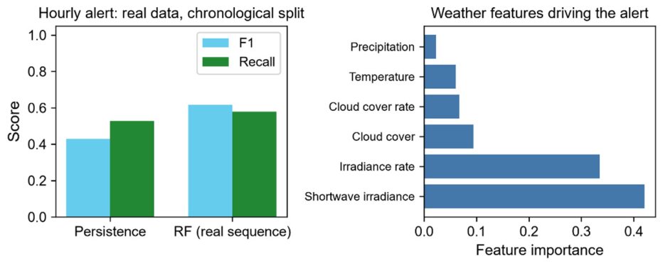
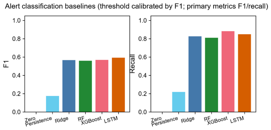
Figure 11. Baseline comparison of warning classification.

4.4. Benchmark Comparison

To substantiate the advantages of the proposed method over existing lines of work, four comparison methods are configured, all adopting the same soft grid-forming operating point $D=20$, so as to isolate the two variables of with/without feedforward and predicted versus measured:

(1)

Fixed droop [2] ($H=2$, $D=20$);

(2)

Adaptive droop coefficient [10] ($D$ switches within $|\Delta f|$ according to $1.5\sim 20$, without feedforward);

(3)

Disturbance-observer feedforward [14] (the deficit is inferred from the measured frequency, with an observation convergence delay of about $0.3 \mathrm{s}$);

(4)

The proposed predictive feedforward (this work).

The results are given in Table 3, and the frequency trajectories of the four methods are compared in Figure 12.

Table 3. Benchmark comparison of the four methods (85% PV drop).

Method	Fast 2 s: Steady State/Nadir/Max RoCoF	Slow 450 s: Steady State
▪ (1) Fixed droop [2]	$48.33/48.33/0.81$	$48.33$
▪ (2) $\mathrm{Adaptive} D$ [10]	$48.33/48.33/0.81$	$48.33$
▪ (3) Observer feedforward [14]	$50.00/49.71/0.70$	$50.00$
▪ (4) Proposed predictive feedforward (this work)	$50.00/50.00/0.17$	$50.00$

Figure 12. Comparison of frequency trajectories for the four methods. The grey droop trajectory coincides with the adaptive-D curve and is therefore hidden beneath it in both panels.

Figure 12. Comparison of frequency trajectories for the four methods. The grey droop trajectory coincides with the adaptive-D curve and is therefore hidden beneath it in both panels.

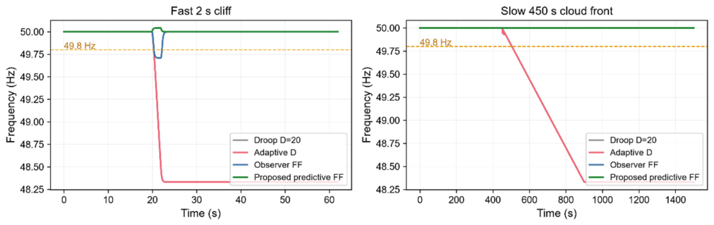
Table 3 reveals two layers of conclusions. First, feedforward eliminates the steady-state deviation: without feedforward, methods (1) and (2) always settle at $48.33 \mathrm{Hz}$ in the steady state (the structural deviation of proportional control; adaptive $D$ only changes the shape of the transient and does not move the steady state), whereas with feedforward, methods (3) and (4) always settle at $50.00 \mathrm{Hz}$. Second, prediction eliminates the fast-transient lag: under a $2 \mathrm{s}$ step drop, method (3) suffers an observer convergence delay of $0.3 \mathrm{s}$ and its frequency nadir is dragged down to $49.71 \mathrm{Hz}$, whereas method (4), by virtue of the warning look-ahead and zero net delay, keeps its nadir at $50.00 \mathrm{Hz}$. In addition, under the slow timescale, method (2) causes $D$ to jump repeatedly between $1.5$ and $20$ because of threshold switching, and the maximum $\mathrm{RoCoF}$ rises instead to $0.223 \mathrm{Hz}/\mathrm{s}$ (far above the $0.004 \mathrm{Hz}/\mathrm{s}$ of fixed droop), which exposes the inherent chattering of measured-frequency-based switching adaptation under ramp conditions; the warning-based predictive pre-raise proposed in this paper does not suffer from this problem. Table 4 further summarizes the qualitative differences among the four control routes.

Table 4. Qualitative comparison of representative control routes.

Route	Refs	Input Signal	Compensation Domain	Timescale	Removes Steady-State Deviation?	Needs Forecast?
▪ Fixed droop/VSG	[2]	Frequency	Frequency	Transient	No	No
▪ Adaptive inertia/damping	[6,8,9,10]	Frequency	Frequency	Transient	No (bounded by 1/D)	No
▪ Forecast-driven reserve/inertia	[12,20]	Solar/weather forecast	Reserve scheduling	Minutes–hour	Partially (reserve, not feedforward)	Yes
▪ Observer/MPC feedforward	[14]	Measured frequency	Power	Transient	Yes, but delayed	No
▪ Load-forecast secondary control	[13]	Load forecast	Secondary loop	Seconds–minutes	Yes (secondary restoration)	Yes
▪ This work	—	Weather warning	Power feedforward + adaptive H/D	Two-timescale	Yes	Yes

Table 4. Qualitative comparison of representative control routes.

Route	Refs	Input Signal	Compensation Domain	Timescale	Removes Steady-State Deviation?	Needs Forecast?
▪ Fixed droop/VSG	[2]	Frequency	Frequency	Transient	No	No
▪ Adaptive inertia/damping	[6,8,9,10]	Frequency	Frequency	Transient	No (bounded by 1/D)	No
▪ Forecast-driven reserve/inertia	[12,20]	Solar/weather forecast	Reserve scheduling	Minutes–hour	Partially (reserve, not feedforward)	Yes
▪ Observer/MPC feedforward	[14]	Measured frequency	Power	Transient	Yes, but delayed	No
▪ Load-forecast secondary control	[13]	Load forecast	Secondary loop	Seconds–minutes	Yes (secondary restoration)	Yes
▪ This work	—	Weather warning	Power feedforward + adaptive H/D	Two-timescale	Yes	Yes

4.5. Ablation Study of the Two Timescales

To verify the division of labor whereby feedforward governs the steady state and adaptive $H/D$ governs the transient, the proposed method is further decomposed into four configurations: droop only; feedforward only ($H$ and $D$ fixed); adaptive $H/D$ only (no feedforward); and the complete method (feedforward plus adaptive $H/D$). The results are given in Table 5 and Figure 13.

Table 5. End-to-end ablation (fast 2 s step drop).

Configuration	Steady State/Nadir/Max RoCoF	Minimum SOC
▪ Droop only	$48.33/48.33/0.81$	$0.4984$
▪ Feedforward only	$50.00/50.00/0.17$	$0.4983$
▪ $\mathrm{Adaptive} H/D$ only	$48.34/48.33/0.80$	$0.4984$
▪ Complete method	$50.00/50.00/0.06$	$0.4983$

Figure 13. End-to-end ablation.

Figure 13. End-to-end ablation.

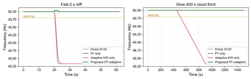
Table 5 clearly shows that the two perform their respective roles and that neither is dispensable: the steady state is determined by feedforward (with feedforward it is $50.00 \mathrm{Hz}$, and adaptive $H/D$ cannot change the steady state); the transient is determined by adaptive $H/D$, and on the same feedforward basis the complete method further compresses ${|\mathrm{RoCoF}|}_{max}$ from $0.17 \mathrm{Hz}/\mathrm{s}$ to $0.06 \mathrm{Hz}/\mathrm{s}$, which is a direct consequence of the inertia pre-raise $2\to 6 \mathrm{s}$ suppressing the residual-driven transient. It should be noted that with adaptive $H/D$ alone, ${|\mathrm{RoCoF}|}_{max}$ remains $0.80 \mathrm{Hz}/\mathrm{s}$, almost identical to fixed droop; the reason is that under a $2 \mathrm{s}$ ramp the frequency follows almost quasi-statically ($\tau =0.196 \mathrm{s}\ll 2 \mathrm{s}$), $\mathrm{RoCoF}$ is dominated by the ramp slope, and $H$ cannot suppress the ramp over the entire disturbance. The value of adaptive $H/D$ materializes only after feedforward has compressed the residual, a mechanism that corroborates the feasible-region conclusion of Section 4.2. Regarding SOC, the minimum SOC of all four configurations is around $0.498$, far above the $0.20$ red line, indicating that feedforward only shifts the active-power reference and does not consume additional ESS capacity [23].

4.6. Compliance Rate and Sensitivity Analysis

Combining Equations (2) and (5), the steady-state frequency deviation of the feedforward system is $\Delta f_{ss}={\displaystyle \frac{f_n\cdot \mathrm{gain}\cdot \epsilon }{D+d_{load}}}$, and compliance (≥49.8 Hz) is equivalent to an amplitude error of $\epsilon \ge -0.1019 \mathrm{p}.\mathrm{u}.$ Let $\epsilon \sim \mathcal{N}\left(0,{\sigma }_{\epsilon }^2\right)$; then the compliance rate is $P=\Phi \left({\displaystyle \frac{0.1019}{{\sigma }_{\epsilon }}}\right)$, and the results for the different ${\sigma }_{\epsilon }$ conventions are given in Table 6 and Figure 14.

Table 6. Dependence of the compliance rate on the prediction-error convention (D = 20).

Convention of the Prediction Error	P (Not Lower than 49.8 Hz)
▪ $0.053$ Overall RMSE	$97.3\%$
▪ $0.064$ Event-level RMSE (real)	$94.4\%$
▪ $0.077$ Persistence baseline	$90.7\%$
▪ $0.100$ Target 0.8 MW	$84.6\%$
▪ $0.151$ Conservative upper bound	$75.0\%$

Figure 14. Joint dependence of the compliance probability.

Figure 14. Joint dependence of the compliance probability.

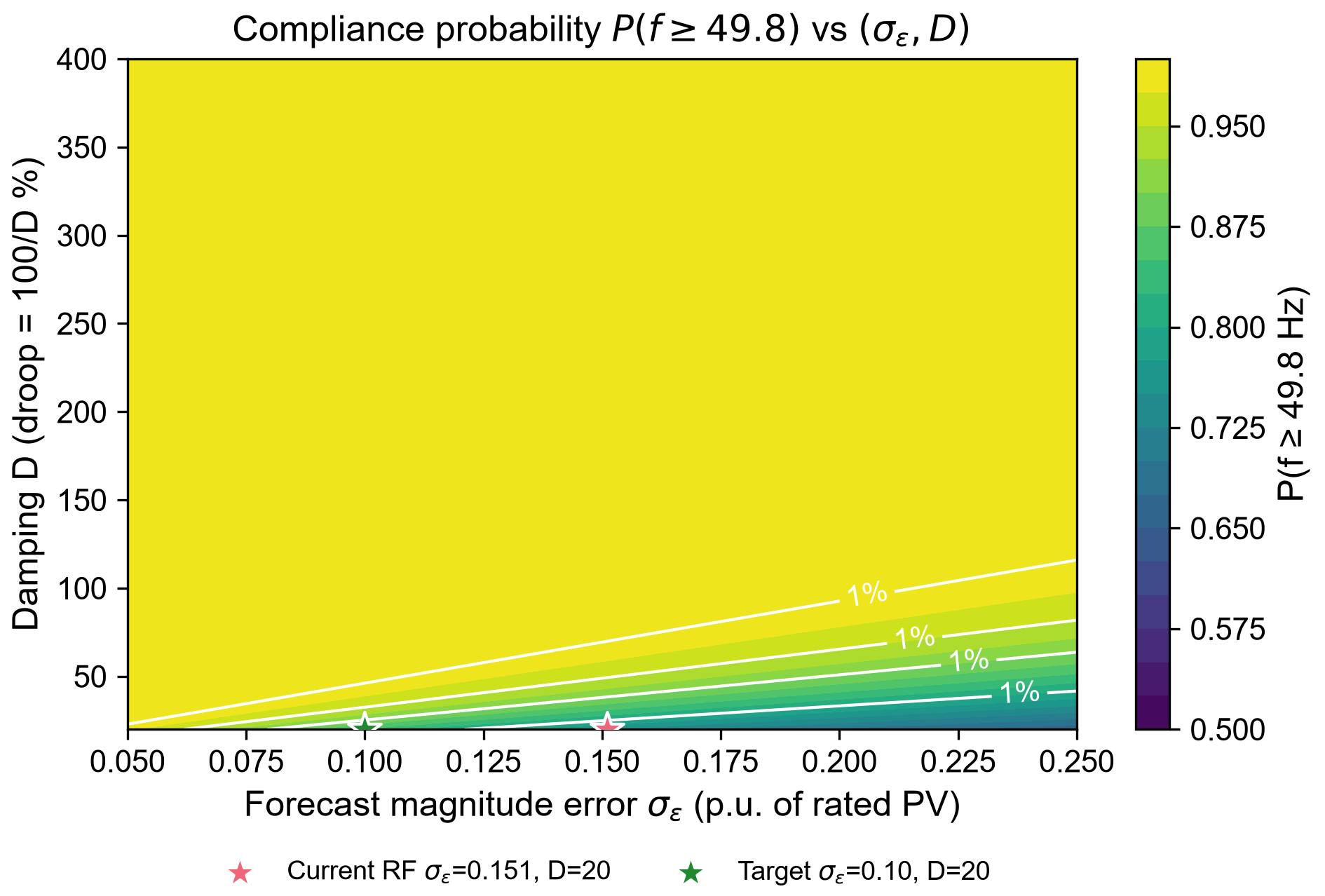
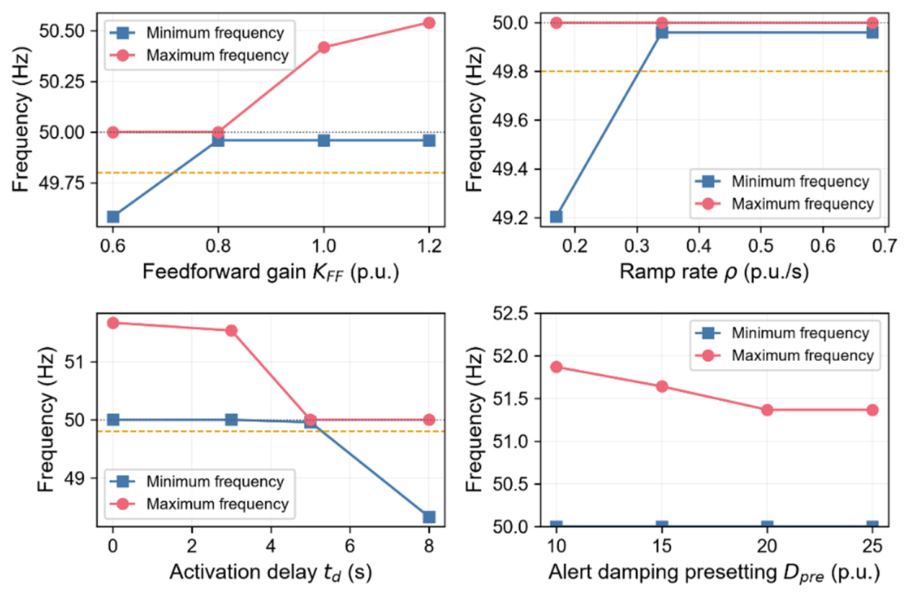
The event-level errors are not exactly Gaussian: for the 302 event samples the skewness is −1.28, the excess kurtosis is +1.71, and the Kolmogorov–Smirnov test rejects normality (D = 0.131, p = 5.5 × 10⁻⁵). After unbiased correction, the compliance rate computed from the empirical event-level distribution is 91.7% (95% bootstrap CI 88.4–94.7%), versus 94.5% under the Gaussian assumption and 94.9% under a fitted t distribution (Table 7). The Gaussian value (94.4%) therefore lies within the 95% CI of the empirical estimate and is mildly optimistic by about 2.8 percentage points; the conclusion is unchanged. Monte Carlo simulations ($200$ runs for each level) agree with the analytical values within the sampling error. This result also reveals an engineering implication: feedforward replaces the main knob for compliance, from the damping $D$ (which is locked by the national standard on the droop ratio and by the deadband) to the prediction accuracy ${\sigma }_{\epsilon }$ (which can be improved by training), and this is the core of the practical value of the method. Finally, a sweep of the feedforward activation delay (Figure 15) shows that setting ${\mathrm{delay}}_s$ equal to the warning look-ahead time produces no transient overshoot and the frequency barely drops during the disturbance, whereas ${\mathrm{delay}}_s=0$ (an advance shift) causes an over-frequency overshoot of about $51.7 \mathrm{Hz}$, indicating that synchronization between the warning instant and the feedforward activation instant is crucial for the transient quality (see also Section 4.7).

Table 7. Sensitivity of the compliance rate to the error-distribution assumption.

Distribution Assumption (After Bias Correction)	P (≥49.8 Hz)
▪ Empirical (event samples)	91.7% (95% CI 88.4–94.7%)
▪ $\mathrm{Gaussian} \mathrm{N}(0, {0.064}^2)$	94.5%
▪ Fitted t (ν = 7.5)	94.9%

Figure 15. Sensitivity to feedforward parameters.The dashed line denotes the 49.8 Hz compliance limit and the dotted line the nominal 50 Hz.

Figure 15. Sensitivity to feedforward parameters.The dashed line denotes the 49.8 Hz compliance limit and the dotted line the nominal 50 Hz.

4.7. Impact of Feedforward Delay

The feedforward controller has an activation delay $t_d$, arising from the warning lead time, communication, and the ramp limiter. To quantify its effect, $t_d$ was swept from 0 to 8 s under the 85% PV drop (Table 8). The frequency nadir remains 50.00 Hz for $t_d\le 3$ s and 49.96 Hz at $t_d=5$ s, but degrades to 48.33 Hz at $t_d=8$ s, i.e., the droop-only level. The mechanism is that the feedforward is effective only while the delay stays below the disturbance-rise timescale; once the delay exceeds it, the compensation arrives after the frequency has already dipped. Since the warning provides a 5 s look-ahead in this study, the measured delay is well within the tolerable range.

Table 8. Frequency nadir versus feedforward activation delay.

Feedforward Delay ${\mathit{t}}_{\mathit{d}}$ (s)	Frequency Nadir (Hz)
▪ 0	50.00
▪ 3	50.00
▪ 5	49.96
▪ 8	48.33

4.8. Comparison with Recent Adaptive-Law Methods

To compare with the most recent adaptive-damping law, the law of [10] (its Equation (28)) was recast in per-unit and run in the same testbed; its gain coefficients were normalized so that the relative variation of the damping coefficient matches that reported in [10]. To keep the adaptation effective, the damping was allowed to rise to 1.5 times its nominal value (up to D = 30) during the transient and returns to D = 20 at steady state. Because the thresholds of [10] are designed for moderate deviations, the comparison is performed at 30% and 50% PV drops; the 30% case matches the 0.6 MW/2 MW disturbance used in [10] (Table 9).

Table 9. Comparison with a recent adaptive-damping law [10] in a common testbed.

PV Drop	Method	Nadir (Hz)	Steady (Hz)
▪ 30%	Fixed droop [2]	49.411	49.411
▪ 30%	Adaptive J/D [10]	49.411	49.411
▪ 30%	Observer feedforward [14]	49.897	50.000
▪ 30%	Proposed (this work)	50.000	50.000
▪ 50%	Fixed droop [2]	49.018	49.018
▪ 50%	Adaptive J/D [10]	49.112	49.152
▪ 50%	Observer feedforward [14]	49.829	50.000
▪ 50%	Proposed (this work)	50.000	50.000

The recent adaptive law improves the steady-state frequency only marginally (49.02 → 49.15 Hz at 50% drop) and provides no measurable improvement at 30% drop, whereas the proposed method reaches 50.00 Hz with a nadir of 50.00 Hz in both cases. This confirms that adaptive inertia/damping acts on the transient and on the effective damping, but cannot structurally eliminate the steady-state deviation; only power-domain feedforward can.

5. Discussion

5.1. Systematic Prediction Bias and Its Correction

According to Table 2, the random forest predictor exhibits a systematic underestimation of $-0.055$ for large-drop events; that is, the predicted amplitude is on average $0.055 \mathrm{p}.\mathrm{u}.$ lower than the actual amplitude (about $0.44 \mathrm{MW}$). This bias does not change the stability conclusion of the feedforward, but it directly erodes the compliance rate. If the uncorrected RF prediction is used directly, the amplitude error $\epsilon$ actually follows $\mathcal{N}\left(-0.055,{0.064}^2\right)$, and the compliance condition $\epsilon \ge -0.1019$ of Section 4.6 yields a compliance rate of $\Phi \left({\displaystyle \frac{0.1019-0.055}{0.064}}\right)=76.8\%$; after an unbiased correction that shifts $\epsilon$ back to $\mathcal{N}\left(0,{0.064}^2\right)$, the compliance rate is restored to $\Phi \left({\displaystyle \frac{0.1019}{0.064}}\right)=94.4\%$. Throughout this paper, 94.4% denotes the Gaussian estimate; the corresponding empirical event-level estimate is 91.7% (Section 4.6).

The two differ by nearly $18$ percentage points, indicating that bias correction is a key step in unlocking the full potential of the feedforward. This correction can be performed online by estimating the mean of historical event errors, and its direction is safe: underestimation only results in insufficient feedforward and a slight frequency dip, and never causes over-frequency, so the correction can be applied gradually without incurring any overshoot risk. Accordingly, the event-level $94.4\%$ in Table 6 of Section 4.6 should be understood as the compliance rate after unbiased correction, while $76.8\%$ is the uncorrected conservative value; together they delineate the performance range of the method under a real predictor.

5.2. Comparison with Online Optimization-Based Scheduling

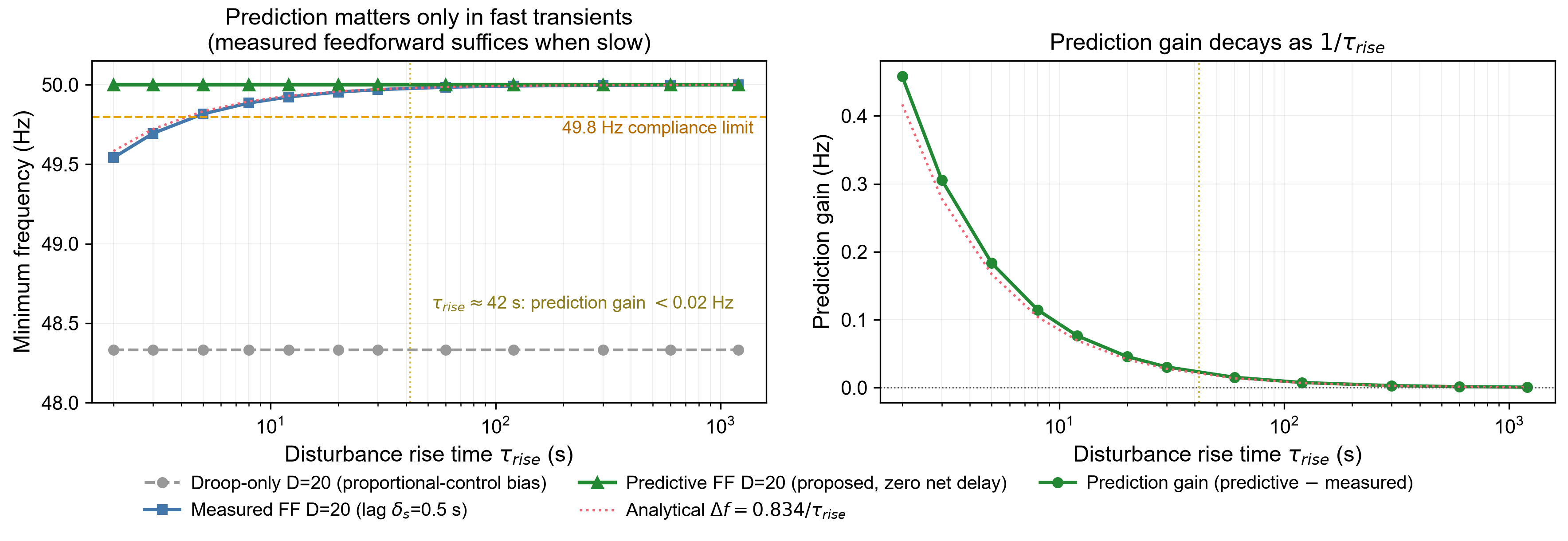
The $H/D$ scheduling in this paper is an analytical solution (Equations (9)–(11)) that requires neither online optimization nor an accurate model, and depends only on the residual bound $\overline{e}$. By contrast, the literature commonly solves $H/D$ online using model predictive control (MPC). Under the simulation settings of this paper and on the same predictive feedforward basis, both the frequency nadir and the maximum $H/D$ of the MPC-based online $\mathrm{RoCoF}$ scheduling are slightly worse than those of the analytical scheduling law, while an optimization problem must also be solved online in every control cycle and the result depends on model accuracy. Figure 16 further shows that the benefit of prediction decays with the disturbance rise time and is material only for fast cloud-front transients.

Figure 16. Decay of the prediction value with the disturbance timescale.

Figure 16. Decay of the prediction value with the disturbance timescale.

The reason is that the residual-driven transient is essentially a first-order process on a short timescale, whose optimal parameters can be given in closed form by Equations (14) and (15); online optimization brings no performance gain while introducing solution delay and model-mismatch risk. This confirms the advantage of the analytical scheduling law derived from the ISS theorem in balancing simplicity, optimality, and robustness: it satisfies both classes of constraints with the tightest parameters, without any numerical optimization.

5.3. Limitations

The proposed method still has several limitations, which define the directions of future work:

First, the modeling adopts a single-machine swing equation and treats the frequency as globally uniform. When extended to multiple grid-forming units, the frequency-power allocation and the consistency among units need to be addressed further [24,25,26,27], although the steady-state conclusion of the feedforward, which depends only on the power balance, is expected to remain valid.

Second, the real meteorological data are hourly, and sub-minute cloud ramps lack direct observation; calibrating ${\sigma }_{\epsilon }$ at the hourly level and applying it to second-level control therefore involves a timescale extrapolation. This paper covers it by means of a $0.06\sim 0.20$ sensitivity sweep, but a more rigorous justification awaits the accumulation of high-time-resolution observation data.

Third, the event-level error is based on only $302$ event samples, and a finer error distribution stratified by drop amplitude remains to be supported by a larger dataset.

Fourth, regarding the influence of warning-timing errors, false alarms, and communication delays on performance, although a confirmation and rollback mechanism has been built into the controller, a systematic experimental evaluation is still insufficient.

Fifth, the voltage-reactive-power loop is treated as quasi-statically decoupled, and the coupled dynamics are not included.

5.4. Applicability to Grid-Connected Operation

The method is formulated for an islanded microgrid in which the grid-forming ESS is the only voltage/frequency master. In grid-connected operation the setting changes in two respects, but the method remains applicable. First, the bulk grid defines the frequency, so the steady-state deviation is no longer set by the local droop loop and the slow-timescale feedforward no longer serves to restore 50 Hz; instead, it shifts the active-power reference ahead of the forecast PV drop, so that the ESS provides primary frequency support with a smaller nadir and a lower RoCoF and with less reliance on the grid reserve. The feedforward law and the residual-based scheduling law remain unchanged, because they act on the power deficit rather than on the absolute frequency. Second, the fast-timescale adaptive H/D remains directly valid: it limits the initial RoCoF and the nadir of the local frequency response within the prescribed thresholds, which is precisely what fast frequency response requires. In weak-grid conditions with a low short-circuit ratio, where the frequency deviation at the point of common coupling is not negligible, the benefit is largest. The method also supports a smooth transition during planned or unplanned islanding, since the ESS is already pre-scheduled before the event. In a stiff grid the local frequency deviation is small and the benefit is correspondingly limited; the method is therefore best suited to weak grids, microgrids, and islanding transitions.

6. Conclusions

Addressing the frequency dip caused by sudden PV drops in islanded microgrids, this paper proposes a two-timescale frequency control method based on meteorological warnings: on the slow timescale, meteorological warnings are used to apply active-power feedforward, compressing the disturbance that droop must compensate from the entire power deficit to the prediction residual; on the fast timescale, virtual inertia and damping are pre-scheduled according to the bound of the prediction residual. The main conclusions are as follows:

(1)

Feedforward eliminates the structural deviation: the feedforward directly removes, in the power domain, the structural steady-state deviation of droop control. Under an 85% PV drop the steady-state frequency is restored from $48.33 \mathrm{Hz}$ to $50.00 \mathrm{Hz}$, and the method is immune to the frequency deadband and robust to the disturbance timescale (Table 3, Figure 12).

(2)

Analytical results and division of labor: an input-to-state stability result is established for the closed-loop system, proving that the frequency deviation is input-to-state stable with respect to the bounded prediction residual. The tightest inertia/damping scheduling law and the feasible residual region ${\overline{e}}_{feas}=0.0815 \mathrm{p}.\mathrm{u}.$ are derived from it, which provides an analytical basis for parameter design and delineates the division of labor between feedforward and adaptive $H/D$ (Proposition 1, Equation (16), Figure 8).

(3)

Validation on measured data and performance improvement: the prediction error is calibrated on three years of hourly measured data from a region in Hubei, giving an event-level ${\sigma }_{\epsilon }=0.064$; the four-method benchmark and the end-to-end ablation verify that feedforward governs the steady state and adaptive $H/D$ governs the transient, and that neither is dispensable. With unbiased correction the steady-state compliance rate ($\ge 49.8\mathrm{Hz}$) reaches 94.4% (Gaussian estimate; 91.7% from the empirical event-level distribution, Section 4.6), and it still reaches $76.8\%$ without correction, far above conventional droop control (Table 2 and Table 7).

Future work will focus on the extension to multiple grid-forming units, the calibration of the prediction error on sub-minute observation data, and robustness against warning-timing errors and false alarms.

References

- Khan, M.; Wu, W.C.; Li, L. Grid-forming control for inverter-based resources in power systems: A review on its operation, system stability, and prospective. IET Renew. Power Gener. 2024, 18, 887–907. [Google Scholar] [CrossRef] [Scilit]
- Zhong, Q.C.; Weiss, G. Synchronverters: Inverters that mimic synchronous generators. IEEE Trans. Ind. Electron. 2011, 58, 1259–1267. [Google Scholar] [CrossRef] [Scilit]
- Lim, S.; Kim, T.; Lee, K.Y.; Choi, D.; Park, J.-W. Impact of high penetration of renewables on power system frequency response: A review and verification. Renew. Sustain. Energy Rev. 2025, 217, 115728. [Google Scholar] [CrossRef] [Scilit]
- Cai, X.; Zhang, N.; Du, E.; An, Z.; Wei, N.; Kang, C. Low inertia power system planning considering frequency quality under high penetration of renewable energy. IEEE Trans. Power Syst. 2024, 39, 4537–4548. [Google Scholar] [CrossRef] [Scilit]
- Yin, H.; Qiu, W.; Wu, Y.; You, S.; Tan, J.; Hoke, A.; Kruse, C.J.; Rockwell, B.W.; Liu, Y. Field measurement and analysis of frequency and RoCoF for low-inertia power systems. IEEE Trans. Ind. Electron. 2024, 71, 7996–8006. [Google Scholar] [CrossRef] [Scilit]
- Song, S.Y.; Han, C.H. Coordinated adaptive droop control of large-scale energy storage systems for primary frequency support in energy management systems. IEEE Trans. Power Syst. 2025, 40, 5302–5311. [Google Scholar] [CrossRef] [Scilit]
- Schneider, K.P.; Sun, X.Q.; Tuffner, F. Adaptive load shedding as part of primary frequency response to support networked microgrid operations. IEEE Trans. Power Syst. 2024, 39, 287–298. [Google Scholar] [CrossRef] [Scilit]
- Kavvathas, T.E.; Konstantopoulos, G.C. Novel virtual synchronous generator design with dynamic virtual inertia and bounded frequency, current and voltage characteristics. IEEE Trans. Sustain. Energy 2026, 17, 620–633. [Google Scholar] [CrossRef] [Scilit]
- Chang, G.W.; Nguyen, K.T. A new adaptive inertia-based virtual synchronous generator with even inverter output power sharing in islanded microgrid. IEEE Trans. Ind. Electron. 2024, 71, 10693–10703. [Google Scholar] [CrossRef] [Scilit]
- Wang, Q.; Zhang, K.; Zhang, Y.; Lin, X.; Yan, W. Adaptive frequency control strategy for grid-forming energy storage based on equivalent active power droop coefficient. J. Electr. Eng. 2026, 21, 398–408. (In Chinese) [Google Scholar]
- Liu, J.H.; Wang, C.; Bi, T.S. RoCoF constrained regional inertia security region: Formulation and application. IEEE Trans. Sustain. Energy 2026, 17, 2514–2529. [Google Scholar] [CrossRef] [Scilit]
- Chang, J.; Du, Y.; Lim, E.G.; Wen, H.; Li, X.; Lin, J. Coordinated frequency regulation using solar forecasting based virtual inertia control for islanded microgrids. IEEE Trans. Sustain. Energy 2021, 12, 2393–2403. [Google Scholar] [CrossRef] [Scilit]
- Shan, Y.H.; Hu, J.F.; Shen, B. Distributed secondary frequency control for AC microgrids using load power forecasting based on artificial neural network. IEEE Trans. Ind. Inform. 2024, 20, 1651–1662. [Google Scholar] [CrossRef] [Scilit]
- Zhong, C.; Zhao, H.; Liu, Y.; Liu, C. Model predictive secondary frequency control of island microgrid based on two-layer moving-horizon estimation observer. Appl. Energy 2024, 372, 123721. [Google Scholar] [CrossRef] [Scilit]
- Al Talaq, M.; Abdelghany, M.B.; Al-Durra, A.; Zeineldin, H.H.; El-Fouly, T.H.M. Optimal configuration and coordinated scheduling of hybrid inverter-based energy sources in large-scale green management systems. IEEE Open J. Ind. Electron. Soc. 2025, 6, 1720–1742. [Google Scholar] [CrossRef] [Scilit]
- Liu, J.; Zang, H.; Ding, T.; Cheng, L.; Wei, Z.; Sun, G. Sky-image-derived deep decomposition for ultra-short-term photovoltaic power forecasting. IEEE Trans. Sustain. Energy 2024, 15, 871–883. [Google Scholar] [CrossRef] [Scilit]
- OuYang, Y.; Guo, Y.; Yang, D.; Tang, J.; Yang, Q.; Jiang, Y.; Qin, L.; Jiang, L. Spectral intermittency regularization for photovoltaic ramp forecasting. Appl. Energy 2026, 426, 128626. [Google Scholar] [CrossRef] [Scilit]
- Zhang, L.W.; Yang, Y.X.; Wu, Y.P. Review of deep learning-based ground-sky imagery method for intra-hour solar irradiance forecasting: Workflow and perspectives. Renew. Sustain. Energy Rev. 2026, 239, 117160. [Google Scholar] [CrossRef] [Scilit]
- Kosmopoulos, P.; Dhake, H.; Melita, N.; Tagarakis, K.; Georgakis, A.; Stefas, A.; Vaggelis, O.; Korre, V.; Kashyap, Y. Multi-layer cloud motion vector forecasting for solar energy applications. Appl. Energy 2024, 353, 122144. [Google Scholar] [CrossRef] [Scilit]
- Bi, T.S.; Liu, J.H.; Wang, C. Online estimation of area-level inertia considering inter-area equivalent frequency dynamics. IEEE Trans. Power Syst. 2025, 40, 57–72. [Google Scholar] [CrossRef] [Scilit]
- Breiman, L. Random forests. Mach. Learn. 2001, 45, 5–32. [Google Scholar] [CrossRef] [Scilit]
- Wang, G.T.; Wang, C.Y.; Shahidehpour, M. Neural network applications in hybrid data-model driven dynamic frequency trajectory prediction for weak-damping power systems. IEEE Trans. Power Syst. 2024, 39, 3227–3239. [Google Scholar] [CrossRef] [Scilit]
- Yan, H.W.; Liang, G.; Beniwal, N.; Rodriguez, E.; Farivar, G.G.; Pou, J. Flexible power point tracking aided power ramp rate control for photovoltaic systems with small energy storage capacity. IEEE Trans. Power Electron. 2024, 39, 2798–2810. [Google Scholar] [CrossRef] [Scilit]
- Ye, P.L. Transient stability analysis of islanded microgrid with parallel grid-forming converters considering current limitation. IEEE Trans. Smart Grid 2026, 17, 3655–3668. [Google Scholar] [CrossRef] [Scilit]
- Ngamroo, I.; Surinkaew, T. Control of distributed converter-based resources in a zero-inertia microgrid using robust deep learning neural network. IEEE Trans. Smart Grid 2024, 15, 49–66. [Google Scholar] [CrossRef] [Scilit]
- Liu, K.; Qian, T.; Zhang, W.; Wu, S.; Han, R.; Hou, K.; Wu, Z.; Hu, Q. Review on small-signal stability of multiple virtual synchronous generators. Renew. Sustain. Energy Rev. 2025, 215, 115543. [Google Scholar] [CrossRef] [Scilit]
- Zhuang, K.; Xin, H.; Chen, H.; Huang, L. Quantitative parameter conditions for stability and coupling in GFM-GFL converter hybrid systems from a small-signal synchronous perspective. IEEE Trans. Sustain. Energy 2026, 17, 2939–2952. [Google Scholar] [CrossRef] [Scilit]
Disclaimer/Publisher’s Note: The statements, opinions and data contained in all publications are solely those of the individual author(s) and contributor(s) and not of MDPI and/or the editor(s). MDPI and/or the editor(s) disclaim responsibility for any injury to people or property resulting from any ideas, methods, instructions or products referred to in the content. |
© 2026 by the authors. Licensee MDPI, Basel, Switzerland. This article is an open access article distributed under the terms and conditions of the Creative Commons Attribution (CC BY) license.