Two Perspectives, One Impedance: Unified dq- and Sequence-Domain Impedance Modeling and Weak-Grid Stability Analysis of Grid-Connected LCL Inverters with Complete Industrial Control Loops

Abstract

Grid-connected inverters with LCL filters regulate the inverter-side current in industrial products. Their small-signal impedance becomes frequency-coupled because of the phase-locked loop (PLL), and the remaining industrial control functions—active damping, PCC voltage feedforward and the outer power loop—make the model more complex. This coupling complicates both the stability assessment in weak grids and the interpretation of the relation between the dq-frame and the sequence-domain representations. This paper develops a unified impedance modeling and sequence-domain transformation framework for such inverters. Instead of complex harmonic linearization, the small-signal dq-frame model is derived in complex-vector form, which reduces the 2 × 2 impedance matrix to scalar sequence impedances without solving coupled multi-frequency algebraic equations. Closed-form relations among the dq, the modified sequence and the coupled sequence impedances are established, and the frequency shift between the two frames is formulated explicitly for both f1 < fc and f1 > fc. The dq-to-sequence equivalence is then verified along two independent routes—one through the stationary alpha–beta frame and one through symmetrical components—and the two results agree. Frequency-domain simulations and measurements on a 215 kW, 690 V industrial product show that the stability margin contracts as the PLL bandwidth widens and that a lead compensator designed from the model restores stable operation in a weak grid.

1. Introduction

Grid-connected voltage-source inverters establish an interface between renewable energy sources and the power system. LCL filters attenuate the switching harmonics but introduce a resonance that must be damped, which is commonly achieved by active damping of the capacitor current [1,2,3,4]. The phase-locked loop (PLL) introduces dq-axis cross-coupling, which makes the impedance asymmetric and creates frequency-domain coupling between the positive- and the negative-sequence components.

Impedance-based stability analysis relies on accurate small-signal models in both the dq and the sequence domains [5,6,7]. The transformation between these two frames involves frequency shifts that complicate impedance measurement and physical interpretation [8,9].

Several sequence-domain impedance definitions and models have been proposed [10,11,12,13,14,15]. The modified sequence-domain impedance definition and its equivalence to the dq-domain impedance were established in [10,16,17], and measurement-oriented sequence-impedance and frequency-scanning formulations were reported in [18,19]. The derivation presented in this paper starts from that framework, but extends and enriches it in three respects: the dq-frame model is obtained through a complex-vector route instead of complex harmonic linearization (CHL) [20], the complete industrial control structure analyzed in Section 2 is retained, and the dq-to-sequence equivalence is proved again from an independent stationary-frame perspective, so that two methods corroborate the same conclusion. The complex-vector representation directly transforms the 2 × 2 dq impedance matrix into scalar sequence impedances, which simplifies both the derivation and the computation while retaining the complete coupling information. The modified sequence impedance keeps a clear physical interpretation and is compatible with the generalized Nyquist criterion for stability assessment [5].

This paper establishes a small-signal impedance model of grid-connected LCL inverters and the transformation that links it to the sequence domain. The main contributions are as follows. (1) A set of impedance models of the complete industrial control structure is derived with a complex-vector representation. Compared with complex harmonic linearization, which is the other main modeling route and requires solving a coupled multi-frequency algebraic system, the complex-vector form yields the sequence impedances directly as scalars and makes the relation between the sequence-domain and the dq-domain impedances transparent. (2) The frequency shift between the rotating and the stationary frames is formulated explicitly for the two regimes f₁ < f_c and f₁ > f_c, and closed-form relations are obtained among the dq impedance, the modified sequence impedance and the coupled sequence impedance. (3) Two independent derivations—one in the stationary alpha–beta frame and one based on symmetrical components—are shown to give the same impedance, which verifies the modified sequence-domain definition for a converter with the full industrial control structure rather than for a reduced model. (4) The model retains the LCL filter, the current control with active damping, the PLL, the PCC voltage feedforward and the outer power loop. Active damping, the feedforward path and the power loop are commonly omitted or simplified, and the controlled variable here is the inverter-side current, as with the industrial product under study, rather than the grid-side current that impedance studies often assume. (5) The framework is validated by frequency-domain simulation and by measurements on a 215 kW, 690 V industrial product, and it is used to quantify the stability margin for different PLL bandwidths and to design a lead compensator that restores stability in a weak grid.

To highlight the contribution of this work with respect to the existing literature, Table 1 compares the proposed approach with representative impedance-modeling methods in terms of the modeling route, the control structure, the impedance domain, and the validation.

Table 1. Comparison of the proposed approach with representative impedance-modeling methods.

Reference	Modeling Route	Control Structure	Impedance Domain	Validation
This work	Complex vector	Complete industrial loops	dq and sequence	Simulation and prototype
Rygg et al. 2016, 2017 [10,16]	Sequence-domain definition	Simplified control loop	dq and sequence	Simulation
Zhang et al. 2018 [17]	Sequence-domain SISO	Simplified control loop	dq and sequence	Simulation
Cespedes and Sun 2014 [20]	Complex harmonic linearization	Simplified control loop	Sequence	Simulation and prototype
Shah et al. 2022 [19]	Sequence-domain MIMO/SISO	Simplified control loop	Sequence	Prototype

The remainder of the paper is organized as follows. Section 2 derives the complete small-signal dq-frame model, including the current loop, the PLL, the active damping, the PCC voltage feedforward and the outer power loop. Section 3 transforms the dq impedance into the sequence domain and establishes its equivalence to the impedance in the stationary alpha–beta frame. Section 4 derives the sequence impedance of the grid-inverter system. Section 5 defines the coupled and the modified sequence admittance and impedance. Section 6 relates the dq impedance to the modified sequence impedance for the two frequency regimes f₁ < f_c and f₁ > f_c. Section 7 describes the corresponding frequency-scanning procedure. Section 8 validates the model by frequency-domain simulation and Section 9 by measurements on a 215 kW industrial product, where the sensitivity to the PLL bandwidth is quantified and a lead compensator is designed. Section 10 concludes the paper. Part of this modeling work was presented in a preliminary form in [21].

2. Modeling of the Grid-Connected LCL Inverter

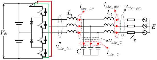
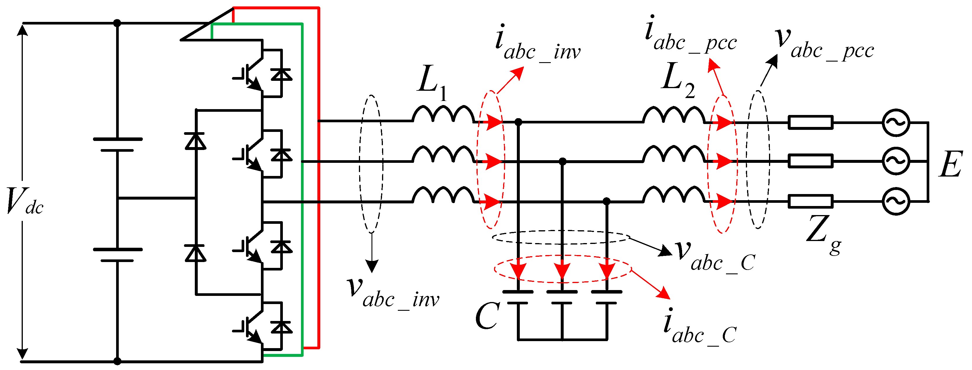
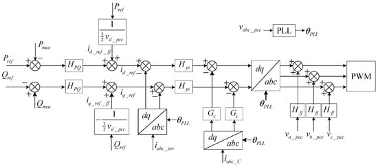
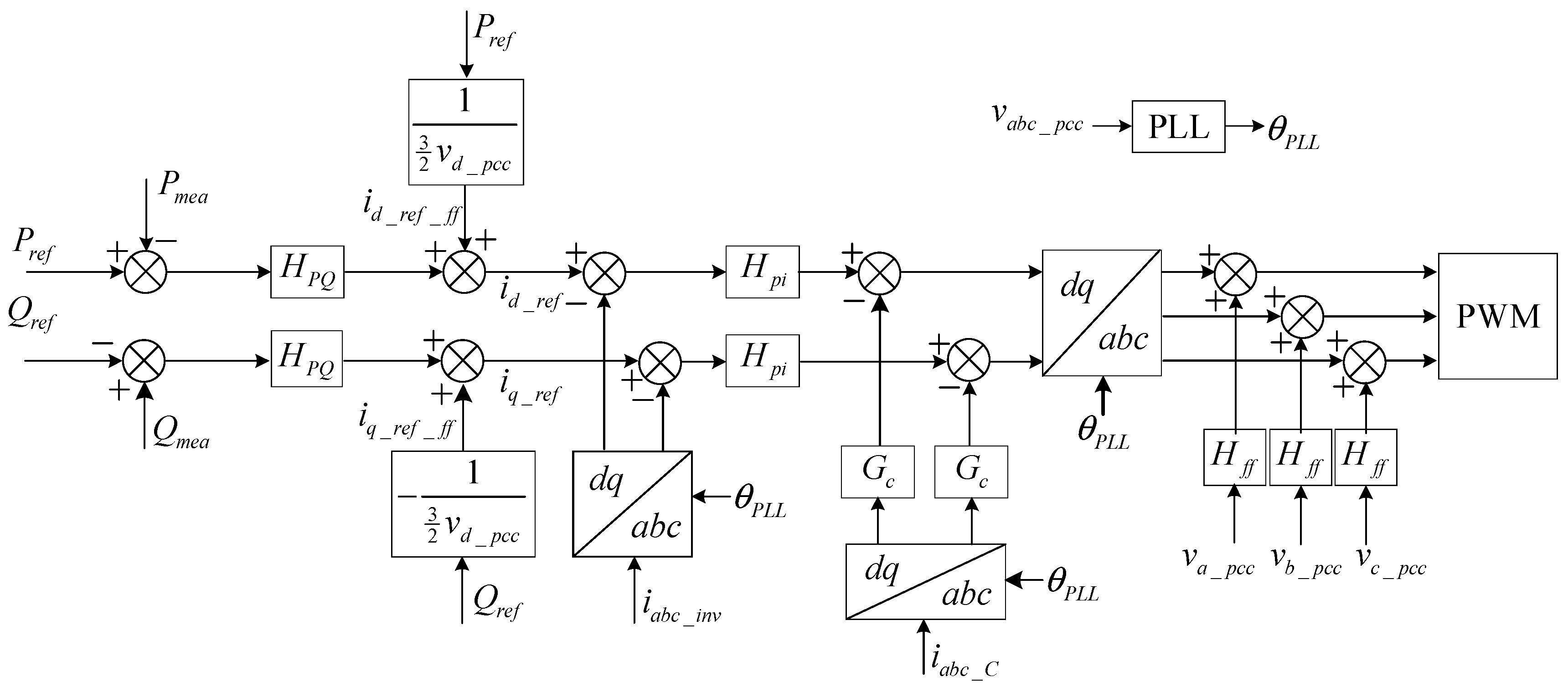
Figure 1 shows the topology of the grid-connected LCL inverter (the explicit hardware parameters are not disclosed here for reasons of commercial confidentiality), and Figure 2 presents the overall control structure. The inverter output current is regulated by the current loop, the filter capacitor current is used for active damping, and the PCC voltage is employed by the PLL and the voltage-feedforward path. These coupled control functions form the basis of the small-signal model derived in this section.

Figure 1. Topology of the grid-connected LCL inverter (215 kW, 690 V).

Figure 2. Overall control structure of the grid-connected inverter.

The parameters in Table 2 define the operating point and the digital implementation. The passive components and the controller gains of the commercial product are not disclosed here for reasons of commercial confidentiality; the model itself is fully parameterized, so the same equations apply to any LCL inverter once its filter, controller and PLL parameters are substituted. The PLL bandwidths used in Section 9 (20, 100 and 200 Hz) and the lead compensator of Section 9.2 (center frequency 200 Hz, maximum lead 40°) are given in the corresponding sections, and the measured impedances reported there provide an independent check of the model.

Table 2. Electrical parameters for modeling the grid-connected inverter.

Electrical Parameters	Value
Grid Frequency	50 Hz
Grid Line Voltage (RMS)	690 V
DC Voltage	1331V
Switching Frequency	16 kHz
Sampling Frequency	32 kHz
Operating Point	P = 215 kW, Q = 0

2.1. LCL Filter Physical Model

Applying Kirchhoff’s voltage law to the grid-side inductor L₂ in the synchronous dq frame [1,7] gives (1).

$$\left[\begin{array}{c}{\stackrel{\wedge }{V}}_{d\_C}\\ {\stackrel{\wedge }{V}}_{q\_C}\end{array}\right]-\left[\begin{array}{c}{\stackrel{\wedge }{V}}_{d\_\mathit{pcc}}\\ {\stackrel{\wedge }{V}}_{q\_\mathit{pcc}}\end{array}\right]=\left[\begin{array}{cc}\mathrm{s}{L}_2& -{\omega }_1{L}_2\\ {\omega }_1{L}_2& s{L}_2\end{array}\right]\left[\begin{array}{c}{\stackrel{\wedge }{I}}_{d\_\mathit{pcc}}\\ {\stackrel{\wedge }{I}}_{q\_\mathit{pcc}}\end{array}\right]$$

(1)

The compact matrix form is given in (2):

$${\widehat{\mathit{V}}}_{\mathit{dq}\_c}-{\widehat{\mathit{V}}}_{\mathit{dq}\_\mathit{pcc}}={\mathit{Z}}_{L2}{\widehat{\mathit{I}}}_{\mathit{dq}\_\mathit{pcc}}$$

(2)

where the grid-side impedance matrix is defined in (3):

$${\mathit{Z}}_{L2}=\left[\begin{array}{cc}{R}_{L2}+\mathrm{s}{L}_2& -{\omega }_1{L}_2\\ {\omega }_1{L}_2& R_{L2}+s{L}_2\end{array}\right]$$

(3)

Similarly, the voltage equation for the converter-side inductor L₁ is given in (4):

$${\widehat{\mathit{V}}}_{\mathit{dq}\_\mathit{inv}}-{\widehat{\mathit{V}}}_{\mathit{dq}\_C}={\mathit{Z}}_{L1}{\widehat{\mathit{I}}}_{\mathit{dq}\_\mathit{inv}}$$

(4)

and the converter-side impedance matrix is defined in (5).

$${\mathit{Z}}_{L1}=\left[\begin{array}{cc}{R}_{L1}+\mathrm{s}{L}_1& -{\omega }_1{L}_1\\ {\omega }_1{L}_1& R_{L1}+s{L}_1\end{array}\right]$$

(5)

For the filter capacitor branch, the current dynamics satisfy (6).

$${\widehat{\mathit{I}}}_{\mathit{dq}\_\mathit{inv}}={\widehat{\mathit{I}}}_{\mathit{dq}\_\mathit{pcc}}+{\widehat{\mathit{I}}}_{\mathit{dq}\_C}={\widehat{\mathit{I}}}_{\mathit{dq}\_\mathit{pcc}}+{\mathit{Y}}_c{\widehat{\mathit{V}}}_{\mathit{dq}\_C}$$

(6)

Combining (2), (4), and (6) gives the terminal voltage–current relationship (7):

$${\widehat{\mathit{V}}}_{\mathit{dq}\_\mathit{inv}}=\underset{A_{\mathit{phys}}}{\underbrace{({\mathit{I}}_2+{\mathit{Z}}_{L1}{\mathit{Y}}_c)}}{\widehat{\mathit{V}}}_{\mathit{dq}\_\mathit{pcc}}+\underset{B_{\mathit{phys}}}{\underbrace{({\mathit{Z}}_{L1}+{\mathit{Z}}_{L2}+{\mathit{Z}}_{L1}{\mathit{Y}}_c{\mathit{Z}}_{L2})}}{\widehat{\mathit{I}}}_{\mathit{dq}\_\mathit{pcc}}$$

(7)

where ${\mathit{I}}_2=\left[\begin{array}{cc}1& 0\\ 0& 1\end{array}\right]$.

2.2. Current-Control Loop

The modulation output M_dq consists of the current PI controller output and the active-damping term [22], as expressed in (8):

$${\widehat{\mathit{M}}}_{\mathit{dq}}=-H_{\mathit{pi}}{\widehat{\mathit{I}}}_{\mathit{dq}\_\mathit{inv}\_\mathit{mea}}-G_c{\widehat{\mathit{I}}}_{\mathit{dq}\_c\_\mathit{mea}}$$

(8)

Applying the inverse Park and Clarke transformations gives (9).

$${\widehat{\mathit{M}}}_{\mathit{abc}}={\mathit{T}}_{\alpha \beta \to \mathit{abc}}{{\mathit{T}}_{\alpha \beta \to \mathrm{dq}}}^{-1}\left({\theta }_{\mathit{PLL}}\right){\widehat{\mathit{M}}}_{\mathit{dq}}$$

(9)

where the modulation angle is defined in (10).

$${\theta }_{\mathit{PLL}}={\omega }_{1}t+\widehat{\theta }$$

(10)

where ω₁ is the grid fundamental angular frequency.

The final modulation signal, including PCC voltage feedforward, is given by (11).

$${\widehat{\mathit{M}}}_{\mathit{abc}\_\mathit{final}}={\widehat{\mathit{M}}}_{\mathit{abc}}+K_{\mathit{ff}}{\widehat{\mathit{V}}}_{\mathit{abc}\_\mathit{pcc}}$$

(11)

The inverter output voltage can then be written as (12).

$${\widehat{\mathit{V}}}_{\mathit{abc}\_\mathit{inv}}=G_{\mathit{pwm}}{\widehat{\mathit{M}}}_{\mathit{abc}\_\mathit{final}}$$

(12)

where G_pwm represents the PWM modulation transfer function, including gain K_pwm and a zero-order hold. The control loop includes 1/K_pwm to cancel the gain, so K_pwm does not appear explicitly in the impedance expression; the resulting transfer function is given in (13).

$$G_{\mathit{PWM}}(s)=e^{-s{T}_s}\cdot G_{\mathit{ZOH}}(s)=e^{-s{T}_s}\cdot {\displaystyle \frac{1-e^{-s{T}_s}}{s{T}_s}}$$

(13)

Substituting the modulation and control relationships into the controller dq frame gives (14).

$$\begin{array}{l}{\widehat{\mathit{V}}}_{\mathit{dq}\_\mathit{inv}\_\mathit{mea}}=G_{\mathit{pwm}}\left(-H_{\mathit{pi}}{\widehat{\mathit{I}}}_{\mathit{dq}\_\mathit{inv}\_\mathit{mea}}-G_c{\widehat{\mathit{I}}}_{\mathit{dq}\_C\_\mathit{mea}}+K_{\mathit{ff}}{\widehat{\mathit{V}}}_{\mathit{dq}\_\mathit{pcc}}\right)\\ =G_{\mathit{pwm}}\left(-H_{\mathit{pi}}{\widehat{\mathit{I}}}_{\mathit{dq}\_\mathit{inv}\_\mathit{mea}}-K_{\mathit{ad}}{\widehat{\mathit{I}}}_{\mathit{dq}\_C\_\mathit{mea}}+K_{\mathit{ff}}{\widehat{\mathit{V}}}_{\mathit{dq}\_\mathit{pcc}}\right)\end{array}$$

(14)

2.3. Small-Signal Frame Transformation

The transformation between the PLL-aligned frame and the system reference frame is given in (15):

$${\widehat{\mathit{V}}}_{\mathit{dq}\_\mathit{inv}\_\mathit{mea}}={\mathit{T}}_{\alpha \beta \to \mathrm{dq}}\left({\theta }_{\mathit{PLL}}\right)\left\{{\mathit{T}}_{\alpha \beta \to \mathrm{dq}}{\left({\omega }_{1}t\right)}^{-1}{\widehat{\mathit{V}}}_{\mathit{dq}\_\mathit{inv}}\right\}$$

(15)

where the rotation matrix is defined in (16), in which J denotes the 90° rotation matrix.

$$\begin{array}{l}{\mathit{T}}_{\alpha \beta \to \mathrm{dq}}\left({\theta }_{\mathit{PLL}}\right){\mathit{T}}_{\alpha \beta \to \mathrm{dq}}{\left({\omega }_{1}t\right)}^{-1}={\mathit{T}}_{\alpha \beta \to \mathrm{dq}}\left({\theta }_{\mathit{PLL}}-{\omega }_{1}t\right)={\mathit{T}}_{\alpha \beta \to \mathrm{dq}}\left(\widehat{\theta }\right)\\ =\left[\begin{array}{cc}\cos \left(\widehat{\theta }\right)& \sin \left(\widehat{\theta }\right)\\ -\sin \left(\widehat{\theta }\right)& \cos \left(\widehat{\theta }\right)\end{array}\right]\approx \left[\begin{array}{cc}1& \widehat{\theta }\\ -\widehat{\theta }& 1\end{array}\right]\\ =\left[\begin{array}{cc}1& 0\\ 0& 1\end{array}\right]-\widehat{\theta }\cdot \left[\begin{array}{cc}0& -1\\ 1& 0\end{array}\right]={\mathit{I}}_2-\widehat{\theta }\cdot \mathit{J}\end{array}$$

(16)

Linearizing (15) around the operating point gives (17).

$$\begin{array}{l}{\overline{\mathit{V}}}_{\mathit{dq}\_\mathit{inv}\_\mathit{mea}}+{\widehat{\mathit{V}}}_{\mathit{dq}\_\mathit{inv}\_\mathit{mea}}=\left({\mathit{I}}_2-\widehat{\theta }J\right)\left({\overline{V}}_{\mathit{dq}\_\mathit{inv}}+{\widehat{\mathit{V}}}_{\mathit{dq}\_\mathit{inv}}\right)\\ ={\overline{V}}_{\mathit{dq}\_\mathit{inv}}+{\widehat{\mathit{V}}}_{\mathit{dq}\_\mathit{inv}}-\widehat{\theta }\mathit{J}{\overline{\mathit{V}}}_{\mathit{dq}\_\mathit{inv}}-\widehat{\theta }J{\widehat{\mathit{V}}}_{\mathit{dq}\_\mathit{inv}}\end{array}$$

(17)

Neglecting second-order small-signal products yields (18).

$${\widehat{\mathit{V}}}_{\mathit{dq}\_\mathit{inv}\_\mathit{mea}}={\widehat{\mathit{V}}}_{\mathit{dq}\_\mathit{inv}}-\widehat{\theta }\mathit{J}{\overline{V}}_{\mathit{dq}\_\mathit{inv}}$$

(18)

The same linearization is applied to the current and voltage measurements, as shown in (19):

$$\begin{array}{l}{\widehat{\mathit{I}}}_{\mathit{dq}\_\mathit{inv}\_\mathit{mea}}={\widehat{\mathit{I}}}_{\mathit{dq}\_\mathit{inv}}-\widehat{\theta }\mathit{J}{\overline{\mathit{I}}}_{\mathit{dq}\_\mathit{inv}}\\ {\widehat{\mathit{I}}}_{\mathit{dq}\_C\_\mathit{mea}}={\widehat{\mathit{I}}}_{\mathit{dq}\_C}-\widehat{\theta }\mathit{J}{\overline{\mathit{I}}}_{\mathit{dq}\_C}\\ {\widehat{\mathit{V}}}_{\mathit{dq}\_\mathit{pcc}\_\mathit{mea}}={\widehat{\mathit{V}}}_{\mathit{dq}\_\mathit{pcc}}-\widehat{\theta }\mathit{J}{\overline{\mathit{V}}}_{\mathit{dq}\_\mathit{pcc}}\end{array}$$

(19)

Substituting (18) and (19) into (14) gives (20):

$$\begin{array}{l}{\widehat{\mathit{V}}}_{\mathit{dq}\_\mathit{inv}}=G_{\mathit{pwm}}\left(-H_{\mathit{pi}}{\widehat{\mathit{I}}}_{\mathit{dq}\_\mathit{inv}}-K_{\mathit{ad}}{\widehat{\mathit{I}}}_{\mathit{dq}\_C}+K_{\mathit{ff}}{\widehat{\mathit{V}}}_{\mathit{dq}\_\mathit{pcc}}\right)\\ +\widehat{\theta }\mathit{J}\left[{\overline{V}}_{\mathit{dq}\_\mathit{inv}}+G_{\mathit{pwm}}\left(H_{\mathit{pi}}{\overline{\mathit{I}}}_{\mathit{dq}\_\mathit{inv}}+K_{\mathit{ad}}{\overline{\mathit{I}}}_{\mathit{dq}\_C}-K_{\mathit{ff}}{\overline{\mathit{V}}}_{\mathit{dq}\_\mathit{pcc}}\right)\right]\\ =G_{\mathit{pwm}}\left(-H_{\mathit{pi}}{\widehat{\mathit{I}}}_{\mathit{dq}\_\mathit{inv}}-K_{\mathit{ad}}{\widehat{\mathit{I}}}_{\mathit{dq}\_C}+K_{\mathit{ff}}{\widehat{\mathit{V}}}_{\mathit{dq}\_\mathit{pcc}}\right)+\widehat{\theta }\mathit{JM}\end{array}$$

(20)

where the matrices are defined in (21).

$$\mathit{M}=\left[{\overline{V}}_{\mathit{dq}\_\mathit{inv}}+G_{\mathit{pwm}}\left(H_{\mathit{pi}}{\overline{\mathit{I}}}_{\mathit{dq}\_\mathit{inv}}+K_{\mathit{ad}}{\overline{\mathit{I}}}_{\mathit{dq}\_C}-K_{\mathit{ff}}{\overline{\mathit{V}}}_{\mathit{dq}\_\mathit{pcc}}\right)\right]$$

(21)

The inverter-side and capacitor currents satisfy (22) and (23).

$${\widehat{\mathit{I}}}_{\mathit{dq}\_\mathit{inv}}={\mathit{Y}}_c{\widehat{\mathit{V}}}_{\mathit{dq}\_C}+{\widehat{\mathit{I}}}_{\mathit{dq}\_\mathit{pcc}}$$

(22)

$${\widehat{\mathit{V}}}_{\mathit{dq}\_C}-{\widehat{\mathit{V}}}_{\mathit{dq}\_\mathit{pcc}}={\mathit{Z}}_{L2}{\widehat{\mathit{I}}}_{\mathit{dq}\_\mathit{pcc}}$$

(23)

Combining (22) and (23) yields (24).

$$\left\{\begin{array}{c}{\widehat{\mathit{I}}}_{\mathit{dq}\_\mathit{inv}}={\mathit{Y}}_c{\widehat{\mathit{V}}}_{\mathit{dq}\_\mathit{pcc}}+\left({\mathit{I}}_2+{\mathit{Y}}_c{\mathit{Z}}_{L2}\right){\widehat{\mathit{I}}}_{\mathit{dq}\_\mathit{pcc}}\\ {\widehat{\mathit{I}}}_{\mathit{dq}\_C}={\mathit{Y}}_c\left({\widehat{\mathit{V}}}_{\mathit{dq}\_\mathit{pcc}}+{\mathit{Z}}_{L2}{\widehat{\mathit{I}}}_{\mathit{dq}\_\mathit{pcc}}\right)\end{array}\right.$$

(24)

Substituting (24) into (20) gives (25).

$$\begin{array}{l}{\widehat{\mathit{V}}}_{\mathit{dq}\_\mathit{inv}}={\mathit{G}}_{\mathit{pwm}}\left(-H_{\mathit{pi}}{\mathit{Y}}_c-K_{\mathit{ad}}{\mathit{Y}}_c+{\mathit{K}}_{\mathit{ff}}\right){\widehat{\mathit{V}}}_{\mathit{dq}\_\mathit{pcc}}\\ +{\mathit{G}}_{\mathit{pwm}}\left(-H_{\mathit{pi}}\left({\mathit{I}}_2+{\mathit{Y}}_c{\mathit{Z}}_{L2}\right)-K_{\mathit{ad}}{\mathit{Y}}_c{\mathit{Z}}_{L2}\right)\cdot {\widehat{\mathit{I}}}_{\mathit{dq}\_\mathit{pcc}}+\widehat{\theta }\mathit{JM}\end{array}$$

(25)

2.4. Phase-Locked Loop Dynamics

The PLL angle deviation appears in the small-signal control equation (25) through the frame rotation [23,24]. To close this loop, the PLL dynamics must be modeled explicitly.

On the one hand, the PLL output angle can be written as (26).

$$\widehat{\theta }(s)={\displaystyle \frac{K_{p\_\mathit{PLL}}+\frac{K_{i\_\mathit{PLL}}}{s}}{s}}E(s)={\displaystyle \frac{K_{p\_\mathit{PLL}}+\frac{K_{i\_\mathit{PLL}}}{s}}{s}}{\widehat{\mathit{V}}}_{q\_\mathit{pcc}\_\mathit{mea}}(s)$$

(26)

On the other hand, the measured PLL input vector can be expressed as (27).

$$\underset{{\widehat{\mathit{V}}}_{\mathit{dq}\_\mathit{pcc}\_\mathit{mea}}}{\underbrace{{\widehat{\mathit{V}}}_{d\_\mathit{pcc}\_\mathit{mea}}+j\cdot {\widehat{\mathit{V}}}_{q\_\mathit{pcc}\_\mathit{mea}}}}=\underset{{\widehat{\mathit{V}}}_{\mathit{dq}\_\mathit{pcc}}}{\underbrace{\left({\widehat{\mathit{V}}}_{d\_\mathit{pcc}}+j\cdot {\widehat{\mathit{V}}}_{q\_\mathit{pcc}}\right)}}-j\cdot \widehat{\theta }\cdot \underset{{{\overline{V}}_{\mathit{dq}\_\mathit{pc}}}_c}{\underbrace{\left({{\overline{V}}_{d\_\mathit{pc}}}_c+j\cdot {{\overline{V}}_{q\_\mathit{pc}}}_c\right)}}$$

(27)

The q-axis component gives (28).

$${\widehat{\mathit{V}}}_{q\_\mathit{pcc}\_\mathit{mea}}\left(s\right)={\widehat{\mathit{V}}}_{q\_\mathit{pcc}}\left(s\right)-{\overline{V}}_{d\_\mathit{pcc}}\cdot \widehat{\theta }\left(s\right)$$

(28)

Substituting (26) into (28) gives (29):

$${\widehat{\mathit{V}}}_{q\_\mathit{pcc}\_\mathit{mea}}\left(s\right)={\widehat{\mathit{V}}}_{q\_\mathit{pcc}}\left(s\right)-{\overline{\mathit{V}}}_{d\_\mathit{pcc}}\cdot {\displaystyle \frac{K_{p\_\mathit{PLL}}+\frac{K_{i\_\mathit{PLL}}}{s}}{s}}\cdot {\widehat{\mathit{V}}}_{q\_\mathit{pcc}\_\mathit{mea}}(s)$$

(29)

which gives (30).

$${\widehat{\mathit{V}}}_{q\_\mathit{pcc}\_\mathit{mea}}(s)={\displaystyle \frac{1}{1+{\overline{V}}_{d\_\mathit{pcc}}\cdot \frac{K_{p\_\mathit{PLL}}+\frac{K_{i\_\mathit{PLL}}}{s}}{s}}}\cdot {\widehat{\mathit{V}}}_{q\_\mathit{pcc}}(s)$$

(30)

Substituting (30) into (26) gives (31):

$$\begin{array}{l}\widehat{\theta }\left(s\right)={\displaystyle \frac{K_p+\frac{K_i}{s}}{s}}{\displaystyle \frac{1}{1+{\overline{V}}_{d\_\mathit{pcc}}\cdot \frac{K_{p\_\mathit{PLL}}+\frac{K_{i\_\mathit{PLL}}}{s}}{s}}}\cdot {\widehat{\mathit{V}}}_{q\_\mathit{pcc}}\left(s\right)\\ ={\displaystyle \frac{G_{\mathit{pll}}\left(s\right)}{s}}{\displaystyle \frac{1}{1+{\overline{V}}_{d\_\mathit{pcc}}\cdot \frac{G_{\mathit{pll}}\left(s\right)}{s}}}\cdot {\widehat{\mathit{V}}}_{q\_\mathit{pcc}}\left(s\right)\\ =T_{\mathit{pll}}\left(s\right)\cdot {\widehat{\mathit{V}}}_{q\_\mathit{pcc}}\left(s\right)\end{array}$$

(31)

where the PLL open-loop transfer function is given in (32).

$$T_{\mathit{pll}}\left(s\right)={\displaystyle \frac{G_{\mathit{pll}}\left(s\right)}{s}}{\displaystyle \frac{1}{1+{\overline{V}}_{d\_\mathit{pcc}}\cdot \frac{G_{\mathit{pll}}\left(s\right)}{s}}}$$

(32)

In vector form, the PLL output is given in (33).

$$\widehat{\theta }=T_{\mathit{pll}}\cdot {\widehat{\mathit{V}}}_{q\_\mathit{pcc}}=T_{\mathit{pll}}\underset{N}{\underbrace{\left[\begin{array}{cc}0& 1\end{array}\right]}}\underset{{\widehat{\mathit{V}}}_{\mathit{dq}\_\mathit{pcc}}}{\underbrace{\left[\begin{array}{c}{\widehat{\mathit{V}}}_{d\_\mathit{pcc}}\\ {\widehat{\mathit{V}}}_{q\_\mathit{pcc}}\end{array}\right]}}$$

(33)

Substituting (33) into (25) gives the closed-loop small-signal model (34):

$$\begin{array}{l}{\widehat{\mathit{V}}}_{\mathit{dq}\_\mathit{inv}}=\underset{A_{\mathit{ctrl}}}{\underbrace{\left[G_{\mathit{pwm}}\left(-H_{\mathit{pi}}{\mathit{Y}}_c-K_{\mathit{ad}}{\mathit{Y}}_c+K_{\mathit{ff}}{\mathit{I}}_2\right)+\mathit{JM}{T}_{\mathit{pll}}\mathit{N}\right]}}{\widehat{\mathit{V}}}_{\mathit{dq}\_\mathit{pcc}}+\\ \underset{B_{\mathit{ctrl}}}{\underbrace{G_{\mathit{pwm}}\left(-H_i\left({\mathit{I}}_2+{\mathit{Y}}_c{\mathit{Z}}_{L2}\right)-K_{\mathit{ad}}{\mathit{Y}}_c{\mathit{Z}}_{L2}\right)}}{\widehat{\mathit{I}}}_{\mathit{dq}\_\mathit{pcc}}\end{array}$$

(34)

2.5. Power Loop

The instantaneous active and reactive powers injected into the grid are defined in (35), and the power control loop affects the low-frequency impedance characteristics [25,26,27].

$$\begin{array}{l}{\overline{\mathit{P}}}_{\mathit{mea}}+{\widehat{\mathit{P}}}_{\mathit{mea}}={\displaystyle \frac{3}{2}}\left[({\widehat{V}}_d+{\overline{V}}_d)({\widehat{I}}_d+{\overline{I}}_d)+({\widehat{V}}_q+{\overline{V}}_q)({\widehat{I}}_q+{\overline{I}}_q)\right]\\ ={\displaystyle \frac{3}{2}}[({\overline{V}}_d{\overline{I}}_d+{\overline{V}}_q{\overline{I}}_q)+({\widehat{V}}_d{\overline{I}}_d+{\overline{V}}_d{\widehat{I}}_d+{\widehat{V}}_q{\overline{I}}_q+{\overline{V}}_q{\widehat{I}}_q)+({\widehat{V}}_d{\widehat{I}}_d+{\widehat{V}}_q{\widehat{I}}_q)]\end{array}$$

(35)

Linearizing (35) and neglecting second-order terms gives the active power increment (36):

$${\widehat{\mathit{P}}}_{\mathit{mea}}={\displaystyle \frac{3}{2}}[{\widehat{V}}_d{\overline{I}}_d+{\overline{V}}_d{\widehat{I}}_d+{\widehat{V}}_q{\overline{I}}_q+{\overline{V}}_q{\widehat{I}}_q]$$

(36)

The reactive power linearization gives (37).

$${\widehat{\mathit{Q}}}_{\mathit{mea}}={\displaystyle \frac{3}{2}}[{\widehat{V}}_q{\overline{I}}_d+{\overline{V}}_q{\widehat{I}}_d-({\widehat{V}}_d{\overline{I}}_q+{\overline{V}}_d{\widehat{I}}_q)]$$

(37)

The active power feedforward term is given in (38).

$$i_{d\_\mathit{ref}\_\mathit{ff}}={\displaystyle \frac{P_{\mathit{ref}}}{\frac{3}{2}{V}_{\mathit{pcc}\_d}}}$$

(38)

Applying first-order Taylor expansion yields (39).

$${\overline{I}}_{d\_\mathit{ref}\_\mathit{ff}}+{\widehat{I}}_{d\_\mathit{ref}\_\mathit{ff}}={\displaystyle \frac{P_{\mathit{ref}}}{\frac{3}{2}{\overline{V}}_{\mathit{pcc}\_d}}}+(-{\displaystyle \frac{P_{\mathit{ref}}}{\frac{3}{2}{{\overline{V}}_{\mathit{pcc}\_d}}^2}}){\widehat{V}}_{\mathit{pcc}\_d}$$

(39)

which gives (40) and (41).

$${\widehat{I}}_{d\_\mathit{ref}\_\mathit{ff}}=(-{\displaystyle \frac{P_{\mathit{ref}}}{\frac{3}{2}{{\overline{V}}_{\mathit{pcc}\_d}}^2}}){\widehat{V}}_{\mathit{pcc}\_d}$$

(40)

and

$${\widehat{I}}_{q\_\mathit{ref}\_\mathit{ff}}=(-{\displaystyle \frac{Q_{\mathit{ref}}}{\frac{3}{2}{{\overline{V}}_{\mathit{pcc}\_d}}^2}}){\widehat{V}}_{\mathit{pcc}\_d}$$

(41)

From Figure 2, the current reference is given in (42).

$$\left\{\begin{array}{c}{\widehat{I}}_{d\_\mathit{ref}}=-H_{\mathit{PQ}}{\widehat{P}}_{\mathit{mea}}+{\widehat{I}}_{d\_\mathit{ref}\_\mathit{ff}}\\ {\widehat{I}}_{q\_\mathit{ref}}=H_{\mathit{PQ}}{\widehat{Q}}_{\mathit{mea}}+{\widehat{I}}_{q\_\mathit{ref}\_\mathit{ff}}\end{array}\right.$$

(42)

The current reference is expressed as a complex vector, as shown in (43):

$$\begin{array}{l}{\widehat{\mathit{I}}}_{\mathit{dq}\_\mathit{ref}}={\widehat{\mathit{I}}}_{d\_\mathit{ref}}+j{\widehat{\mathit{I}}}_{q\_\mathit{ref}}\\ =-H_{\mathit{PQ}}{\widehat{P}}_{\mathit{mea}}+{\widehat{I}}_{d\_\mathit{ref}\_\mathit{ff}}+j(H_{\mathit{PQ}}{\widehat{Q}}_{\mathit{mea}}+{\widehat{I}}_{q\_\mathit{ref}\_\mathit{ff}})\end{array}$$

(43)

Including the power-loop contribution, the inverter voltage equation (14) becomes (44):

$$\begin{array}{l}{\widehat{\mathit{V}}}_{\mathit{dq}\_\mathit{inv}\_\mathit{mea}}=G_{\mathit{pwm}}\left(-H_{\mathit{pi}}({\widehat{\mathit{I}}}_{\mathit{dq}\_\mathit{inv}\_\mathit{mea}}-{\widehat{\mathit{I}}}_{\mathit{dq}\_\mathit{ref}})-G_c{\widehat{\mathbf{I}}}_{\mathit{dq}\_C\_\mathit{mea}}+K_{\mathit{ff}}{\widehat{V}}_{\mathit{dq}\_\mathit{pcc}}\right)\\ =G_{\mathit{pwm}}\left(-H_{\mathit{pi}}({\widehat{\mathit{I}}}_{\mathit{dq}\_\mathit{inv}\_\mathit{mea}}-{\widehat{\mathit{I}}}_{\mathit{dq}\_\mathit{ref}})-K_{\mathit{ad}}{\widehat{\mathbf{I}}}_{\mathit{dq}\_C\_\mathit{mea}}+K_{\mathit{ff}}{\widehat{V}}_{\mathit{dq}\_\mathit{pcc}}\right)\end{array}$$

(44)

Substituting (36), (37), (40), and (41) into (43), and then (43) into (44), gives the closed-form current reference that incorporates the power-loop dynamics into the dq-frame impedance model.

In (35)–(43), an overbar denotes the steady-state value and a hat denotes the small-signal increment, and products of increments are neglected after linearization. The sign convention is that positive current flows from the inverter into the grid, and an increase in the PCC voltage reduces the current reference through the feedforward path; this is why the feedforward terms in (40) and (41) carry a negative sign.

2.6. dq-Frame Impedance Model

Combining (7) with the closed-loop control model (34) and (44) gives (45).

$$\begin{array}{l}{\widehat{\mathit{V}}}_{\mathit{dq}\_\mathit{inv}\_\mathit{ideal}}=A_{\mathit{phys}}{\widehat{\mathit{V}}}_{\mathit{dq}\_\mathit{pcc}}+B_{\mathit{phys}}{\widehat{\mathit{I}}}_{\mathit{dq}\_\mathit{pcc}}\\ {\widehat{\mathit{V}}}_{\mathit{dq}\_\mathit{inv}\_\mathit{ideal}}=A_{\mathit{ctrl}}{\widehat{\mathit{V}}}_{\mathit{dq}\_\mathit{pcc}}+B_{\mathit{ctrl}}{\widehat{\mathit{I}}}_{\mathit{dq}\_\mathit{pcc}}\end{array}$$

(45)

Defining positive current flow from the inverter into the grid gives (46):

$$Z_{\mathit{dq}}=-{\widehat{\mathit{V}}}_{\mathit{dq}\_\mathit{pcc}}{{\widehat{\mathit{I}}}_{\mathit{dq}\_\mathit{pcc}}}^{-1}$$

(46)

Combining (34) and the LCL filter model (7) gives the final dq-frame impedance expression (47):

$$Z_{\mathit{dq}}=-{\left(A_{\mathit{ctrl}}-A_{\mathit{phys}}\right)}^{-1}\left(B_{\mathit{phys}}-B_{\mathit{ctrl}}\right)$$

(47)

where Z_dq is the 2 × 2 impedance matrix defined in (48).

$$\left[\begin{array}{c}{v}_d\\ v_q\end{array}\right]=\left[\begin{array}{cc}{Z}_{\mathit{dd}}(s)& Z_{\mathit{dq}}(s)\\ Z_{\mathit{qd}}(s)& Z_{\mathit{qq}}(s)\end{array}\right]\left[\begin{array}{c}{i}_d\\ i_q\end{array}\right]$$

(48)

2.7. Complex-Space Representation and Stationary-Frame Transformation

All four elements of the dq impedance matrix are identified by injecting positive- and negative-sequence perturbations, as expressed in (49) and (50):

$$\left[\begin{array}{c}{v}_{d+}{(s)}_{+}\\ v_{q+}{(s)}_{+}\end{array}\right]=\left[\begin{array}{cc}{Z}_{\mathit{dd}}(s)& Z_{\mathit{dq}}(s)\\ Z_{\mathit{qd}}(s)& Z_{\mathit{qq}}(s)\end{array}\right]\left[\begin{array}{c}{i}_{d+}{(s)}_{+}\\ i_{q+}{(s)}_{+}\end{array}\right]$$

(49)

$$\left[\begin{array}{c}{v}_{d+}{(s)}_{-}\\ v_{q+}{(s)}_{-}\end{array}\right]=\left[\begin{array}{cc}{Z}_{\mathit{dd}}(s)& Z_{\mathit{dq}}(s)\\ Z_{\mathit{qd}}(s)& Z_{\mathit{qq}}(s)\end{array}\right]\left[\begin{array}{c}{i}_{d+}{(s)}_{-}\\ i_{q+}{(s)}_{-}\end{array}\right]$$

(50)

In this notation, the first subscript denotes the reference axis, i.e., the positive or the negative sequence, and the second denotes the direction of the perturbation current.

When the dq control is symmetrical (Z_dd = Z_qq and Z_dq = −Z_qd), the dq variables reduce to the complex scalar representation (51):

v_dq = (Z_dd + jZ_qd)i_dq

(51)

For asymmetrical dq channels, the complex-space transformation of [7,8] gives (52)–(54):

$$\left\{\begin{array}{c}\left[\begin{array}{c}{i}_{\mathit{dq}}\\ {i^{*}}_{\mathit{dq}}\end{array}\right]=\left[\begin{array}{cc}1& j\\ 1& -j\end{array}\right]\left[\begin{array}{c}{i}_d\\ i_q\end{array}\right]\\ \left[\begin{array}{c}{v}_{\mathit{dq}}\\ {v^{*}}_{\mathit{dq}}\end{array}\right]=\left[\begin{array}{cc}1& j\\ 1& -j\end{array}\right]\left[\begin{array}{c}{v}_d\\ v_q\end{array}\right]\end{array}\right.$$

(52)

Substituting (52) into (49) or (50) gives (53) and (54):

$${\left[\begin{array}{cc}1& j\\ 1& -j\end{array}\right]}^{-1}\left[\begin{array}{c}{v}_{\mathit{dq}}\\ {v^{*}}_{\mathit{dq}}\end{array}\right]=\left[\begin{array}{cc}{Z}_{\mathit{dd}}& Z_{\mathit{dq}}\\ Z_{\mathit{qd}}& Z_{\mathit{qq}}\end{array}\right]{\left[\begin{array}{cc}1& j\\ 1& -j\end{array}\right]}^{-1}\left[\begin{array}{c}{i}_{\mathit{dq}}\\ {i^{*}}_{\mathit{dq}}\end{array}\right]$$

(53)

And

$$\left[\begin{array}{c}{v}_{\mathit{dq}}\\ {v^{*}}_{\mathit{dq}}\end{array}\right]=\left[\begin{array}{cc}1& j\\ 1& -j\end{array}\right]\left[\begin{array}{cc}{Z}_{\mathit{dd}}& Z_{\mathit{dq}}\\ Z_{\mathit{qd}}& Z_{\mathit{qq}}\end{array}\right]{\left[\begin{array}{cc}1& j\\ 1& -j\end{array}\right]}^{-1}\left[\begin{array}{c}{i}_{\mathit{dq}}\\ {i^{*}}_{\mathit{dq}}\end{array}\right]$$

(54)

Expanding the matrix product gives (55).

$$\begin{array}{l}\left[\begin{array}{c}{v}_{\mathit{dq}}(s)\\ {v^{*}}_{\mathit{dq}}(s)\end{array}\right]=\left[\begin{array}{cc}{\displaystyle \frac{Z_{\mathit{dd}}+Z_{\mathit{qq}}}{2}}+j{\displaystyle \frac{Z_{\mathit{qd}}-Z_{\mathit{dq}}}{2}}& {\displaystyle \frac{Z_{\mathit{dd}}-Z_{\mathit{qq}}}{2}}+j{\displaystyle \frac{Z_{\mathit{qd}}+Z_{\mathit{dq}}}{2}}\\ {\displaystyle \frac{Z_{\mathit{dd}}-Z_{\mathit{qq}}}{2}}-j{\displaystyle \frac{Z_{\mathit{qd}}+Z_{\mathit{dq}}}{2}}& {\displaystyle \frac{Z_{\mathit{dd}}+Z_{\mathit{qq}}}{2}}-j{\displaystyle \frac{Z_{\mathit{qd}}-Z_{\mathit{dq}}}{2}}\end{array}\right]\left[\begin{array}{c}{i}_{\mathit{dq}}(s)\\ {i^{*}}_{\mathit{dq}}(s)\end{array}\right]\\ =\left[\begin{array}{cc}{Z}_{\mathit{dq}+}(s)& Z_{\mathit{dq}-}(s)\\ {Z^{*}}_{\mathit{dq}-}(s)& {Z^{*}}_{\mathit{dq}+}(s)\end{array}\right]\left[\begin{array}{c}{i}_{\mathit{dq}}(s)\\ {i^{*}}_{\mathit{dq}}(s)\end{array}\right]\end{array}$$

(55)

Expressing (55) in the stationary alpha–beta frame introduces a frequency modulation, as given in (56), where the frequency-shift factor has been applied and the asterisk denotes complex conjugation, i.e., the real part is unchanged and the sign of the imaginary part is reversed:

$$\left[\begin{array}{c}{v}_{\alpha \beta }(s)e^{-j{\omega }_{1}t}\\ \mathit{conjugate}(v_{\alpha \beta }(s)e^{-j{\omega }_{1}t})\end{array}\right]=\left[\begin{array}{c}{v}_{\alpha \beta }(s)e^{-j{\omega }_{1}t}\\ {v_{\alpha \beta }}^{*}(s)e^{j{\omega }_{1}t}\end{array}\right]=\left[\begin{array}{cc}{Z}_{\mathit{dq}+}(s-j{\omega }_n)& Z_{\mathit{dq}-}(s-j{\omega }_n)\\ {Z^{*}}_{\mathit{dq}-}(s-j{\omega }_n)& {Z^{*}}_{\mathit{dq}+}(s-j{\omega }_n)\end{array}\right]\left[\begin{array}{c}{i}_{\alpha \beta }(s)e^{-j{\omega }_{1}t}\\ {i_{\alpha \beta }}^{*}(s)e^{j{\omega }_{1}t}\end{array}\right]$$

(56)

It can be expanded as (57):

$$\left\{\begin{array}{c}{v}_{\alpha \beta }(s)e^{-j{\omega }_{1}t}=Z_{\mathit{dq}+}(s-j{\omega }_n)i_{\alpha \beta }(s)e^{-j{\omega }_{1}t}+Z_{\mathit{dq}-}(s-j{\omega }_n){i_{\alpha \beta }}^{*}(s)e^{j{\omega }_{1}t}\\ {v_{\alpha \beta }}^{*}(s)e^{j{\omega }_{1}t}={Z^{*}}_{\mathit{dq}-}(s-j{\omega }_n)i_{\alpha \beta }(s)e^{-j{\omega }_{1}t}+{Z^{*}}_{\mathit{dq}+}(s-j{\omega }_n){i_{\alpha \beta }}^{*}(s)e^{j{\omega }_{1}t}\end{array}\right.$$

(57)

and simplified to (58):

$$\left\{\begin{array}{c}{v}_{\alpha \beta }(s)=Z_{\mathit{dq}+}(s-j{\omega }_1)i_{\alpha \beta }(s)+Z_{\mathit{dq}-}(s-j{\omega }_1){i_{\alpha \beta }}^{*}(s)e^{j2{\omega }_{1}t}\\ {v_{\alpha \beta }}^{*}(s)e^{j2{\omega }_{1}t}={Z^{*}}_{\mathit{dq}-}(s-j{\omega }_1)i_{\alpha \beta }(s)+{Z^{*}}_{\mathit{dq}+}(s-j{\omega }_1){i_{\alpha \beta }}^{*}(s)e^{j2{\omega }_{1}t}\end{array}\right.$$

(58)

Applying the frequency shift then gives (59):

$$\left\{\begin{array}{c}{v}_{\alpha \beta }(s)=Z_{\mathit{dq}+}(s-j{\omega }_1)i_{\alpha \beta }(s)+Z_{\mathit{dq}-}(s-j{\omega }_1){i_{\alpha \beta }}^{*}(s-2j{\omega }_1)\\ {v_{\alpha \beta }}^{*}(s-2j{\omega }_1)={Z^{*}}_{\mathit{dq}-}(s-j{\omega }_1)i_{\alpha \beta }(s)+{Z^{*}}_{\mathit{dq}+}(s-j{\omega }_1){i_{\alpha \beta }}^{*}(s-2j{\omega }_1)\end{array}\right.$$

(59)

The sequence-domain impedance in terms of the stationary-frame variables is therefore given in (60).

$$\left[\begin{array}{c}{v}_{\alpha \beta }(s)\\ {v_{\alpha \beta }}^{*}(s-2j{\omega }_1)\end{array}\right]=\left[\begin{array}{cc}{Z}_{\mathit{dq}+}(s-j{\omega }_1)& Z_{\mathit{dq}-}(s-j{\omega }_1)\\ {Z^{*}}_{\mathit{dq}-}(s-j{\omega }_1)& {Z^{*}}_{\mathit{dq}+}(s-j{\omega }_1)\end{array}\right]\left[\begin{array}{c}{i}_{\alpha \beta }(s)\\ {i_{\alpha \beta }}^{*}(s-2j{\omega }_n)\end{array}\right]$$

(60)

2.8. Steady-State Operating Point

The steady-state dq vectors are determined by the PCC voltage and the active/reactive power dispatch, as given in (61)–(63):

$${\overline{\mathit{V}}}_{\mathit{dq}\_c}={\overline{\mathit{V}}}_{\mathit{dq}\_\mathit{pcc}}+{\mathit{Z}}_{L2}{\overline{\mathit{I}}}_{\mathit{dq}\_\mathit{pcc}}$$

(61)

$${\overline{\mathit{I}}}_{\mathit{dq}\_\mathit{inv}}={\overline{\mathit{I}}}_{\mathit{dq}\_c}+{\overline{\mathit{I}}}_{\mathit{dq}\_\mathit{pcc}}$$

(62)

$${\overline{\mathit{I}}}_{\mathit{dq}\_C}=Y_{\mathit{dq}\_C}{\overline{\mathit{V}}}_{\mathit{dq}\_C}$$

(63)

Solving (61)–(63) for the filter capacitor voltage gives (64).

$${\overline{\mathit{V}}}_{\mathit{dq}\_C}={\left({\mathit{I}}_2+{\mathit{Z}}_{L2}{\mathit{Y}}_c\right)}^{-1}\left({\overline{\mathit{V}}}_{\mathit{dq}\_\mathit{pcc}}+{\mathit{Z}}_{L2}{\overline{\mathit{I}}}_{\mathit{dq}\_\mathit{inv}}\right)$$

(64)

Solving for the steady-state inverter bridge voltage gives (65):

$$\begin{array}{l}{\overline{\mathit{V}}}_{\mathit{dq}\_\mathit{inv}}={\overline{\mathit{V}}}_{\mathit{dq}\_C}+{\mathit{Z}}_{L1}{\overline{\mathit{I}}}_{\mathit{dq}\_\mathit{inv}}\\ ={\left(I_2+{\mathit{Z}}_{L2}{\mathit{Y}}_c\right)}^{-1}\left({\overline{\mathit{V}}}_{\mathit{dq}\_\mathit{pcc}}+{\mathit{Z}}_{L1}{\overline{\mathit{I}}}_{\mathit{dq}\_\mathit{inv}}\right)+{\mathit{Z}}_{L1}{\overline{\mathit{I}}}_{\mathit{dq}\_\mathit{inv}}\end{array}$$

(65)

Substituting the steady-state quantities into the matrix M in (34) completes the small-signal dq-frame output-impedance model.

3. Transformation from the dq Frame to the Sequence Domain

The transformation below follows the modified sequence-domain impedance definition of [10,16] and the sequence-domain SISO equivalent models of [17], which are extended here to the complete industrial control structure modeled in Section 2. Using symmetrical-component theory, the positive- and negative-sequence voltages are given in (66). Throughout the paper, f₁ and f_c are frequencies in hertz, ω₁ = 2πf₁ and ω_c = 2πf_c are the corresponding angular frequencies in rad/s, and s = jω is the Laplace variable; a frequency shift is therefore written as s ± jω₁ in the Laplace domain and as f ± f₁ in the frequency domain.

$$\left[\begin{array}{c}{v}_p\left(t\right)\\ v_n\left(t\right)\end{array}\right]={\displaystyle \frac{1}{3}}\left[\begin{array}{ccc}1& a& a^2\\ 1& a^2& a\end{array}\right]\left[\begin{array}{c}{v}_a\left(t\right)\\ v_b\left(t\right)\\ v_c\left(t\right)\end{array}\right]$$

(66)

where a is the complex phase-shift operator, and (67) holds.

$$a=e^{j{\displaystyle \frac{2}{3}}\pi }$$

(67)

The three-phase voltages expressed in the synchronous dq frame are given in (68).

$$\left[\begin{array}{c}{v}_a\left(t\right)\\ v_b\left(t\right)\\ v_c\left(t\right)\end{array}\right]=\left[\begin{array}{cc}\cos \mathit{\theta }& -\sin \mathit{\theta }\\ \cos \left(\theta -\frac{2}{3}\pi \right)& -\sin \left(\theta -\frac{2}{3}\pi \right)\\ \cos \left(\theta +\frac{2}{3}\pi \right)& -\sin \left(\theta +\frac{2}{3}\pi \right)\end{array}\right]\left[\begin{array}{c}{v}_d\left(t\right)\\ v_q\left(t\right)\end{array}\right]$$

(68)

Substituting (68) into (66) gives the positive-sequence component (69):

$$\begin{array}{l}\overrightarrow{v_p}={\displaystyle \frac{1}{3}}\left[v_a\left(t\right)+a\cdot v_b\left(t\right)+a^2\cdot v_c\left(t\right)\right]\\ ={\displaystyle \frac{1}{3}}\left[\begin{array}{l}\left(v_d\left(t\right)\cdot \cos \mathit{\theta }-v_q\left(t\right)\cdot \sin \mathit{\theta }\right)\\ +a\left(v_d\left(t\right)\cdot \cos \left(\theta -\frac{2}{3}\pi \right)-v_q\left(t\right)\cdot \sin \left(\theta -\frac{2}{3}\pi \right)\right)\\ +a^2\left(v_d\left(t\right)\cdot \cos \left(\theta +\frac{2}{3}\pi \right)-v_q\left(t\right)\cdot \sin \left(\theta +\frac{2}{3}\pi \right)\right)\end{array}\right]\\ ={\displaystyle \frac{1}{3}}\left[\overrightarrow{v_d}\cdot \left({\displaystyle \frac{3}{2}}{e}^{\mathit{j\theta }}\right)-\overrightarrow{v_q}\cdot \left(-j{\displaystyle \frac{3}{2}}{e}^{\mathit{j\theta }}\right)\right]\\ ={\displaystyle \frac{1}{2}}{e}^{\mathit{j\theta }}\left(\overrightarrow{v_d}+j\cdot \overrightarrow{v_q}\right)\end{array}$$

(69)

To express (69) in vector form, it can be rewritten as (70):

$${\mathit{V}}_p={\displaystyle \frac{1}{2}}{e}^{\mathit{j\theta }}\left({\mathit{V}}_d+j\cdot {\mathit{V}}_q\right)$$

(70)

The negative-sequence component follows similarly in (71):

$${\mathit{V}}_n={\displaystyle \frac{1}{2}}{e}^{-\mathit{j\theta }}\left({\mathit{V}}_d-j\cdot {\mathit{V}}_q\right)$$

(71)

After demodulating the carrier-frequency terms, the complex sequence components are given in (72):

$$\left\{\begin{array}{c}{\mathit{V}}_p={\displaystyle \frac{1}{2}}\left[{\mathit{V}}_d+j\cdot {\mathit{V}}_q\right]\\ {\mathit{V}}_n={\displaystyle \frac{1}{2}}\left[{\mathit{V}}_d-j\cdot {\mathit{V}}_q\right]\end{array}\right.$$

(72)

The matrix form is given in (73):

$$\left[\begin{array}{c}{\mathit{V}}_p\\ {\mathit{V}}_n\end{array}\right]=\underset{T_{\mathit{dq}\to \mathit{pn}}}{\underbrace{{\displaystyle \frac{1}{2}}\left[\begin{array}{cc}1& j\\ 1& -j\end{array}\right]}}\left[\begin{array}{c}{\mathit{V}}_d\\ {\mathit{V}}_q\end{array}\right]=T_{\mathit{dq}\to \mathit{pn}}\left[\begin{array}{c}{\mathit{V}}_d\\ {\mathit{V}}_q\end{array}\right]$$

(73)

Incorporating the frequency shift between the dq and sequence frames, (73) can be rewritten as (74):

$$\left[\begin{array}{c}{\mathit{V}}_p(s+j{\omega }_1)\\ {\mathit{V}}_n(s-j{\omega }_1)\end{array}\right]=\underset{T_{\mathit{dq}\to \mathit{pn}}}{\underbrace{{\displaystyle \frac{1}{2}}\left[\begin{array}{cc}1& j\\ 1& -j\end{array}\right]}}\left[\begin{array}{c}{\mathit{V}}_d\\ {\mathit{V}}_q\end{array}\right]=T_{\mathit{dq}\to \mathit{pn}}\left[\begin{array}{c}{\mathit{V}}_d(s)\\ {\mathit{V}}_q(s)\end{array}\right]$$

(74)

The sequence-domain quantities then follow from the dq quantities as (75):

$$\left\{\begin{array}{c}{\mathit{V}}_{\mathit{pn}}=T_{\mathit{dq}\to \mathit{pn}}\cdot {\mathit{V}}_{\mathit{dq}}\\ {\mathit{I}}_{\mathit{pn}}=T_{\mathit{dq}\to \mathit{pn}}\cdot {\mathit{I}}_{\mathit{dq}}\end{array}\right.$$

(75)

Substituting (75) into (76) and eliminating the dq variables (77) gives the sequence-domain impedance matrix (78):

V_pn = Z_pn ⋅ I_pn

(76)

T_dq→pnV_dq = Z_pnT_dq→pnI_dq

(77)

$${\mathit{Z}}_{\mathit{pn}}={\mathit{T}}_{\mathit{dq}\to \mathit{pn}}\underset{Z_{\mathit{dq}}}{\underbrace{{\mathit{V}}_{\mathit{dq}}{{\mathit{I}}_{\mathit{dq}}}^{-1}}}{\mathit{T}}_{\mathit{pn}\to \mathit{dq}}={\mathit{T}}_{\mathit{dq}\to \mathit{pn}}{\mathit{Z}}_{\mathit{dq}}{\mathit{T}}_{\mathit{pn}\to \mathit{dq}}$$

(78)

Expanding (78) gives (79).

$$\begin{array}{l}\left[\begin{array}{cc}{Z}_{\mathit{pp}}& Z_{\mathit{pn}}\\ Z_{\mathit{np}}& Z_{\mathit{nn}}\end{array}\right]={\displaystyle \frac{1}{2}}\left[\begin{array}{cc}1& j\\ 1& -j\end{array}\right]\left[\begin{array}{cc}{Z}_{\mathit{dd}}& Z_{\mathit{dq}}\\ Z_{\mathit{qd}}& Z_{\mathit{qq}}\end{array}\right]\left[\begin{array}{cc}1& 1\\ -j& j\end{array}\right]\\ =\left[\begin{array}{cc}{\displaystyle \frac{Z_{\mathit{dd}}+Z_{\mathit{qq}}}{2}}+j{\displaystyle \frac{Z_{\mathit{qd}}-Z_{\mathit{dq}}}{2}}& {\displaystyle \frac{Z_{\mathit{dd}}-Z_{\mathit{qq}}}{2}}+j{\displaystyle \frac{Z_{\mathit{qd}}+Z_{\mathit{dq}}}{2}}\\ {\displaystyle \frac{Z_{\mathit{dd}}-Z_{\mathit{qq}}}{2}}-j{\displaystyle \frac{Z_{\mathit{qd}}+Z_{\mathit{dq}}}{2}}& {\displaystyle \frac{Z_{\mathit{dd}}+Z_{\mathit{qq}}}{2}}-j{\displaystyle \frac{Z_{\mathit{qd}}-Z_{\mathit{dq}}}{2}}\end{array}\right]\end{array}$$

(79)

The modified sequence impedance is therefore defined as in (80).

$$\left[\begin{array}{c}{V}_p\\ V_n\end{array}\right]={\mathit{Z}}_{\mathit{pn}}\left[\begin{array}{c}{I}_p\\ I_n\end{array}\right]=\left[\begin{array}{cc}{Z}_{\mathit{pp}}& Z_{\mathit{pn}}\\ Z_{\mathit{np}}& Z_{\mathit{nn}}\end{array}\right]\left[\begin{array}{c}{I}_p\\ I_n\end{array}\right]$$

(80)

The dq-to-sequence result of (79) and (80) coincides with the result obtained in the stationary alpha–beta frame in (60), even though the two derivations start from different representations. This agreement confirms that the modified sequence impedance and the impedance seen in the stationary alpha–beta frame are the same quantity, and it is the central analytical result of this section.

Frequency Shift Between dq and Sequence Frames

The rotating dq frame and the stationary sequence frame differ by the frequency shift given in (74) and (75); therefore, (81) follows.

$$\left[\begin{array}{c}{V}_p(s+j{\omega }_1)\\ V_n(s-j{\omega }_1)\end{array}\right]={\mathit{Z}}_{\mathit{pn}}(s)\left[\begin{array}{c}{I}_p(s+j{\omega }_1)\\ I_n(s-j{\omega }_1)\end{array}\right]=\left[\begin{array}{cc}{Z}_{\mathit{pp}}(s)& Z_{\mathit{pn}}(s)\\ Z_{\mathit{np}}(s)& Z_{\mathit{nn}}(s)\end{array}\right]\left[\begin{array}{c}{I}_p(s+j{\omega }_1)\\ I_n(s-j{\omega }_1)\end{array}\right]$$

(81)

Equation (81) gives the modified sequence impedance directly in the dq perturbation-frequency domain. When s = 0, the model reduces to the fundamental-frequency impedance.

4. Sequence Impedance of the Grid-Inverter System

Let superscripts I and G denote the inverter-side and the grid-side quantities, respectively. For a symmetrical grid, injecting a positive-sequence perturbation current at the PCC gives the network equations derived from Kirchhoff’s laws; applying the appropriate frequency shift to the positive- and the negative-sequence models, respectively, then gives (82) and (83):

$$Z_p^I(s)=Z_{\mathit{pp}}^I(s-j{\omega }_1)-{\displaystyle \frac{Z_{\mathit{pn}}^I(s-j{\omega }_1)Z_{\mathit{np}}^I(s-j{\omega }_1)}{Z_{\mathit{nn}}^G(s-j{\omega }_1)+Z_{\mathit{nn}}^I(s-j{\omega }_1)}}$$

(82)

$$Z_n^I(s)=Z_{\mathit{nn}}^I(s+j{\omega }_1)-{\displaystyle \frac{Z_{\mathit{np}}^I(s+j{\omega }_1)Z_{\mathit{pn}}^I(s+j{\omega }_1)}{Z_{\mathit{pp}}^G(s+j{\omega }_1)+Z_{\mathit{pp}}^I(s+j{\omega }_1)}}$$

(83)

Equations (82) and (83) show that both grid impedance coupling and asymmetric dq control contribute to the frequency-coupled impedance.

5. Coupled and Modified Sequence Impedance and Admittance

The modified sequence impedance (80) can equivalently be expressed in admittance form [17,28] as (84).

$$\left[\begin{array}{c}{I}_p(s+j{\omega }_1)\\ I_n(s-j{\omega }_1)\end{array}\right]=\left[\begin{array}{cc}{Y}_{\mathit{pp}}(s)& Y_{\mathit{pn}}(s)\\ Y_{\mathit{np}}(s)& Y_{\mathit{nn}}(s)\end{array}\right]\left[\begin{array}{c}{V}_p(s+j{\omega }_1)\\ V_n(s-j{\omega }_1)\end{array}\right]$$

(84)

When a positive-sequence voltage perturbation Vp(s + jω1) is injected, both a positive-sequence current Ip(s + jω1) and a coupled negative-sequence current In(s − jω1) are produced. Similarly, a negative-sequence perturbation Vn(s − jω1) produces Ip(s + jω1) and In(s − jω1). The coupled admittance equations are therefore:

$$\left\{\begin{array}{l}{I}_p(s+j{\omega }_1)=Y_{\mathit{pp}}(s)V_p(s+j{\omega }_1)\\ I_n(s-j{\omega }_1)=Y_{\mathit{np}}(s)V_p(s+j{\omega }_1)\end{array}\right.$$

(85)

$$\left\{\begin{array}{l}{I}_p(s+j{\omega }_1)=Y_{\mathit{pn}}(s)V_n(s-j{\omega }_1)\\ I_n(s-j{\omega }_1)=Y_{\mathit{nn}}(s)V_n(s-j{\omega }_1)\end{array}\right.$$

(86)

Solving (85) and (86) for the admittance elements gives (87):

$$\left\{\begin{array}{l}{Y}_{\mathit{pp}}(s)={\displaystyle \frac{I_p(s+j{\omega }_1)}{V_p(s+j{\omega }_1)}},Y_{\mathit{pn}}(s)={\displaystyle \frac{I_p(s+j{\omega }_1)}{V_n(s-j{\omega }_1)}}\\ Y_{\mathit{np}}(s)={\displaystyle \frac{I_n(s-j{\omega }_1)}{V_p(s+j{\omega }_1)}},Y_{\mathit{nn}}(s)={\displaystyle \frac{I_n(s-j{\omega }_1)}{V_n(s-j{\omega }_1)}}\end{array}\right.$$

(87)

The coupled sequence admittance for a single-frequency perturbation is given in (88).

$$\left\{\begin{array}{l}{Y}_p(s)={\displaystyle \frac{I_p(s)}{V_p(s)}},Y_{\mathit{cp}}(s)={\displaystyle \frac{I_n(s-j2{\omega }_1)}{V_p(s)}}\\ Y_n(s)={\displaystyle \frac{I_n(s)}{V_n(s)}},Y_{\mathit{cn}}(s)={\displaystyle \frac{I_p(s+j2{\omega }_1)}{V_n(s)}}\end{array}\right.$$

(88)

The modified and coupled sequence admittances are related by (89).

$$\left\{\begin{array}{l}{Y}_p(s)=Y_{\mathit{pp}}(s-j{\omega }_1),Y_{\mathit{cp}}(s)=Y_{\mathit{np}}(s-j{\omega }_1)\\ Y_n(s)=Y_{\mathit{nn}}(s+j{\omega }_1),Y_{\mathit{cn}}(s)=Y_{\mathit{pn}}(s+j{\omega }_1)\end{array}\right.$$

(89)

The corresponding coupled sequence impedance is given in (90).

$$\left\{\begin{array}{l}{Z}_p(s)={\displaystyle \frac{1}{Y_p(s)}}={\displaystyle \frac{1}{Y_{\mathit{pp}}(s-j{\omega }_1)}},Z_{\mathit{cp}}(s)={\displaystyle \frac{1}{Y_{\mathit{cp}}(s)}}={\displaystyle \frac{1}{Y_{\mathit{np}}(s-j{\omega }_1)}}\\ Z_n(s)={\displaystyle \frac{1}{Y_n(s)}}={\displaystyle \frac{1}{Y_{\mathit{nn}}(s+j{\omega }_1)}},Z_{\mathit{cn}}(s)={\displaystyle \frac{1}{Y_{\mathit{cn}}(s)}}={\displaystyle \frac{1}{Y_{\mathit{pn}}(s+j{\omega }_1)}}\end{array}\right.$$

(90)

Because the sequence impedance and admittance matrices are full matrix inverses, their diagonal entries are not simply reciprocals of one another, as (91) shows.

$$\left\{\begin{array}{l}{Z}_p(s)={\displaystyle \frac{1}{Y_{\mathit{pp}}(s-j{\omega }_1)}}\ne Z_{\mathit{pp}}(s-j{\omega }_1),Z_{\mathit{cp}}(s)={\displaystyle \frac{1}{Y_{\mathit{np}}(s-j{\omega }_1)}}\ne Z_{\mathit{np}}(s-j{\omega }_1)\\ Z_n(s)={\displaystyle \frac{1}{Y_{\mathit{nn}}(s+j{\omega }_1)}}\ne Z_{\mathit{nn}}(s+j{\omega }_1),Z_{\mathit{cn}}(s)={\displaystyle \frac{1}{Y_{\mathit{pn}}(s+j{\omega }_1)}}\ne Z_{\mathit{pn}}(s+j{\omega }_1)\end{array}\right.$$

(91)

The coupled sequence impedance and admittance are intermediate representations used to separate the measurement into frequency responses. They are not directly measurable physical impedances. The modified sequence impedance (80) is the physically meaningful quantity for stability analysis.

6. Relationship Between dq and Modified Sequence Impedances

In the stationary frame, a dq-frame perturbation at the frequency f_c appears at f₁ + f_c and at |f₁ − f_c|, where f₁ is the fundamental frequency. Two frequency regimes therefore arise, depending on whether fc is below or above f₁.

6.1. Case 1: f₁ < f_c

For f₁ < fc, the two coupled frequencies f₁ + fc and fc − f₁ are both positive, so both a positive- and a negative-sequence perturbation can be applied, as listed in Table 3.

Table 3. Sequence-domain test cases for f1 < fc.

Test	Disturbance Voltage	Positive-Sequence Response	Negative-Sequence Response
A	f1 + fc (positive sequence)	f1 + fc	fc − f1
B	fc − f1 (negative sequence)	f1 + fc	fc − f1

Using the test configurations in Table 3, the measured sequence admittance is obtained from (80), as expressed in (92):

$${\mathit{Y}}_{\mathit{pn}\_\mathit{mea}}=\left[\begin{array}{cc}{Y}_{\mathit{pp}\_\mathit{mea}}& Y_{\mathit{pn}\_\mathit{mea}}\\ Y_{\mathit{np}\_\mathit{mea}}& Y_{\mathit{nn}\_\mathit{mea}}\end{array}\right]=-\left[\begin{array}{cc}{I}_{\mathit{pA}\_\mathit{mea}}& I_{\mathit{pB}\_\mathit{mea}}\\ I_{\mathit{nA}\_\mathit{mea}}& I_{\mathit{nB}\_\mathit{mea}}\end{array}\right]\cdot {\left[\begin{array}{cc}{V}_{\mathit{pA}\_\mathit{mea}}& V_{\mathit{pB}\_\mathit{mea}}\\ V_{\mathit{nA}\_\mathit{mea}}& V_{\mathit{nB}\_\mathit{mea}}\end{array}\right]}^{-1}=-{\mathit{I}}_{\mathit{pn}\_\mathit{mea}}/{\mathit{V}}_{\mathit{pn}\_\mathit{mea}}$$

(92)

Because the perturbation voltages satisfy (93),

$${\left[\begin{array}{cc}{V}_{\mathit{pA}\_\mathit{mea}}& V_{\mathit{pB}\_\mathit{mea}}\\ V_{\mathit{nA}\_\mathit{mea}}& V_{\mathit{nB}\_\mathit{mea}}\end{array}\right]}^{-1}={\displaystyle \frac{1}{V_{\mathit{pA}\_\mathit{mea}}{V}_{\mathit{nB}\_\mathit{mea}}-V_{\mathit{pB}\_\mathit{mea}}{V}_{\mathit{nA}\_\mathit{mea}}}}\left[\begin{array}{cc}{V}_{\mathit{nB}\_\mathit{mea}}& -V_{\mathit{pB}\_\mathit{mea}}\\ -V_{\mathit{nA}\_\mathit{mea}}& V_{\mathit{pA}\_\mathit{mea}}\end{array}\right]$$

(93)

the inverse of the voltage matrix follows as (94).

$${\mathit{Y}}_{\mathit{pn}\_\mathit{mea}}={\displaystyle \frac{1}{V_{\mathit{pA}\_\mathit{mea}}{V}_{\mathit{nB}\_\mathit{mea}}-V_{\mathit{pB}\_\mathit{mea}}{V}_{\mathit{nA}\_\mathit{mea}}}}\left[\begin{array}{cc}{I}_{\mathit{pB}\_\mathit{mea}}{V}_{\mathit{nA}\_\mathit{mea}}-I_{\mathit{pA}\_\mathit{mea}}{V}_{\mathit{nB}\_\mathit{mea}}& I_{\mathit{pA}\_\mathit{mea}}{V}_{\mathit{pB}\_\mathit{mea}}-I_{\mathit{pB}\_\mathit{mea}}{V}_{\mathit{pA}\_\mathit{mea}}\\ I_{\mathit{nB}\_\mathit{mea}}{V}_{\mathit{nA}\_\mathit{mea}}-I_{\mathit{nA}\_\mathit{mea}}{V}_{\mathit{nB}\_\mathit{mea}}& I_{\mathit{nA}\_\mathit{mea}}{V}_{\mathit{pB}\_\mathit{mea}}-I_{\mathit{nB}\_\mathit{mea}}{V}_{\mathit{pA}\_\mathit{mea}}\end{array}\right]$$

(94)

The individual elements of the measured sequence admittance are therefore given in (95).

$$\left\{\begin{array}{c}{Y}_{\mathit{pp}\_\mathit{mea}}={\displaystyle \frac{I_{\mathit{pB}\_\mathit{mea}}{V}_{\mathit{nA}\_\mathit{mea}}-I_{\mathit{pA}\_\mathit{mea}}{V}_{\mathit{nB}\_\mathit{mea}}}{V_{\mathit{pA}\_\mathit{mea}}{V}_{\mathit{nB}\_\mathit{mea}}-V_{\mathit{pB}\_\mathit{mea}}{V}_{\mathit{nA}\_\mathit{mea}}}}\\ Y_{\mathit{pn}\_\mathit{mea}}={\displaystyle \frac{I_{\mathit{pA}\_\mathit{mea}}{V}_{\mathit{pB}\_\mathit{mea}}-I_{\mathit{pB}\_\mathit{mea}}{V}_{\mathit{pA}\_\mathit{mea}}}{V_{\mathit{pA}\_\mathit{mea}}{V}_{\mathit{nB}\_\mathit{mea}}-V_{\mathit{pB}\_\mathit{mea}}{V}_{\mathit{nA}\_\mathit{mea}}}}\\ Y_{\mathit{np}\_\mathit{mea}}={\displaystyle \frac{I_{\mathit{nB}\_\mathit{mea}}{V}_{\mathit{nA}\_\mathit{mea}}-I_{\mathit{nA}\_\mathit{mea}}{V}_{\mathit{nB}\_\mathit{mea}}}{V_{\mathit{pA}\_\mathit{mea}}{V}_{\mathit{nB}\_\mathit{mea}}-V_{\mathit{pB}\_\mathit{mea}}{V}_{\mathit{nA}\_\mathit{mea}}}}\\ Y_{\mathit{nn}\_\mathit{mea}}={\displaystyle \frac{I_{\mathit{nA}\_\mathit{mea}}{V}_{\mathit{pB}\_\mathit{mea}}-I_{\mathit{nB}\_\mathit{mea}}{V}_{\mathit{pA}\_\mathit{mea}}}{V_{\mathit{pA}\_\mathit{mea}}{V}_{\mathit{nB}\_\mathit{mea}}-V_{\mathit{pB}\_\mathit{mea}}{V}_{\mathit{nA}\_\mathit{mea}}}}\end{array}\right.$$

(95)

The modified sequence admittance is then obtained as (96).

$${\mathit{Y}}_{\mathit{pn}\_\mathrm{mod}}=\left[\begin{array}{cc}{Y}_{\mathit{pp}}& Y_{\mathit{pn}}\\ Y_{\mathit{np}}& Y_{\mathit{nn}}\end{array}\right]={\mathit{Y}}_{\mathit{pn}\_\mathit{mea}}=\left[\begin{array}{cc}{Y}_{\mathit{pp}\_\mathit{mea}}& Y_{\mathit{pn}\_\mathit{mea}}\\ Y_{\mathit{np}\_\mathit{mea}}& Y_{\mathit{nn}\_\mathit{mea}}\end{array}\right]$$

(96)

6.2. Case 2: f₁ > f_c

For f₁ > f_c, the test configurations in Table 4 are used, and the modified sequence admittance is extracted as (97).

Y_{pn_mea} = −I_{pn_mea}/V_{pn_mea}

(97)

and therefore the admittance relation becomes (98).

$${\mathit{Y}}_{\mathit{pn}\_\mathit{mea}}=\left[\begin{array}{cc}{Y}_{\mathit{pp}\_\mathit{mea}}& Y_{\mathit{pn}\_\mathit{mea}}\\ Y_{\mathit{np}\_\mathit{mea}}& Y_{\mathit{nn}\_\mathit{mea}}\end{array}\right]$$

(98)

Table 4. Sequence-domain test cases for f1 > fc.

Test	Disturbance Voltage	Positive-Sequence Response	Mirror Component
A	f1 + fc (positive sequence)	f1 + fc	f1 − fc
B	f1 − fc (positive sequence)	f1 + fc	f1 − fc

The reconstructed modified sequence admittance is given in (99).

$${\mathit{Y}}_{\mathit{seq}\_\mathrm{mod}}=\left[\begin{array}{cc}{Y}_{\mathit{pp}}& Y_{\mathit{pn}}\\ Y_{\mathit{np}}& Y_{\mathit{nn}}\end{array}\right]=\left[\begin{array}{cc}{Y}_{\mathit{pp}\_\mathit{mea}}& Y_{\mathit{pn}\_\mathit{mea}}\\ {Y_{\mathit{np}\_\mathit{mea}}}^{*}& {Y_{\mathit{nn}\_\mathit{mea}}}^{*}\end{array}\right]$$

(99)

The corresponding modified sequence impedance is given in (100).

$${\mathit{Z}}_{\mathit{seq}}={{\mathit{Y}}_{\mathit{seq}}}^{-1}$$

(100)

Transforming this result back to dq coordinates gives (101).

Y_dq = T_pn→dq ⋅ Y_pn ⋅ T_dq→pn, Z_dq = Y_dq⁻¹

(101)

7. Frequency-Scanning Procedure for Coupled Sequence Impedance

The coupled sequence impedance is obtained by injecting perturbations at the PCC while the inverter is connected to an ideal voltage source, i.e., with the grid impedance set to zero, following the measurement practice described in [12,18,19]. The procedure below applies to the two frequency regimes defined in Section 6, and the resulting coupled sequence impedance is given in (102).

$$\left\{\begin{array}{l}{Z}_p(s)={\displaystyle \frac{V_p(s)}{I_p(s)}},{\mathrm{Z}}_{\mathit{cp}}(s)={\displaystyle \frac{V_p(s)}{I_n(s-j2{\omega }_1)}}\\ Z_n(s)={\displaystyle \frac{V_n(s)}{I_n(s)}},Z_{\mathit{cn}}(s)={\displaystyle \frac{V_n(s)}{I_p(s+j2{\omega }_1)}}\end{array}\right.$$

(102)

7.1. Positive-Sequence Scan

Inject a positive-sequence voltage perturbation at f = f_p.

Extract the terminal voltage V_p(f_p) and current I_p(f_p) by FFT, as in (103):

$$Z_p(f_p)={\displaystyle \frac{V_p(f_p)}{I_p(f_p)}}$$

(103)

When f_p < 2f₁, extract the mirror component I_p(2f₁ − f_p), as given in (104):

$$Z_{\mathit{cp}}(f_p)={\displaystyle \frac{V_p(f_p)}{{I_p}^{*}(2f_1-f_p)}}$$

(104)

When f_p ≥ 2f₁, the coupled response I_n(f_p − 2f₁) appears directly, and the coupled impedance follows from (105):

$$Z_{\mathit{cp}}(f_p)={\displaystyle \frac{V_p(f_p)}{I_n(f_p-2f_1)}}$$

(105)

Repeat the procedure over the target frequency grid.

7.2. Negative-Sequence Scan

Inject a negative-sequence voltage perturbation at f = f_n.

Extract V_n(f_n) and I_n(f_n) by FFT, as in (106):

$$Z_n(f_n)={\displaystyle \frac{V_n(f_n)}{I_n(f_n)}}$$

(106)

Extract the coupled positive-sequence current Ip(fn + 2f1), as given in (107):

$$Z_{\mathit{cn}}(f_n)={\displaystyle \frac{V_n(f_n)}{I_p(f_n+2f_1)}}$$

(107)

Repeat the procedure over the target frequency grid.

Equations (1)–(107) together form the final model. The LCL filter and the frame transformation give the terminal voltage–current relation (1)–(7); the current control, active damping and feedforward produce the modulation voltage (8)–(14); the PLL and the frame rotation close the loop (15)–(34); the power loop provides the current reference (35)–(44); and the dq-frame impedance (45)–(48) is then transformed, first into the stationary alpha–beta frame (49)–(60) and then, through symmetrical components, into the sequence domain (66)–(81). The grid coupling (82)–(83), the admittance relations (84)–(91) and the measurement extraction (92)–(107) complete the model used for validation.

8. Simulation Verification

8.1. Verification Without Power Loop

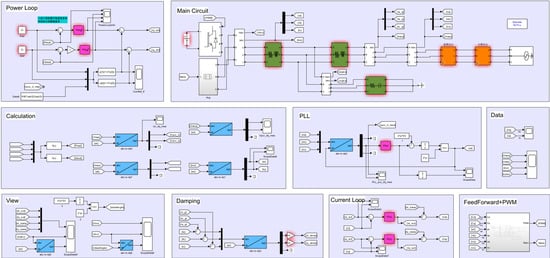
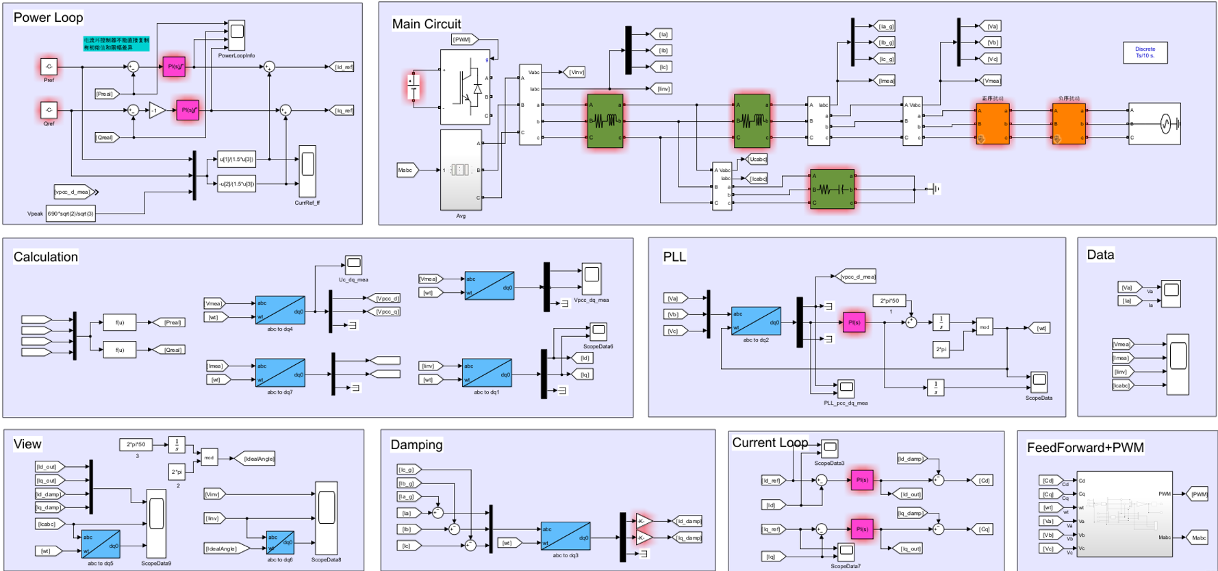
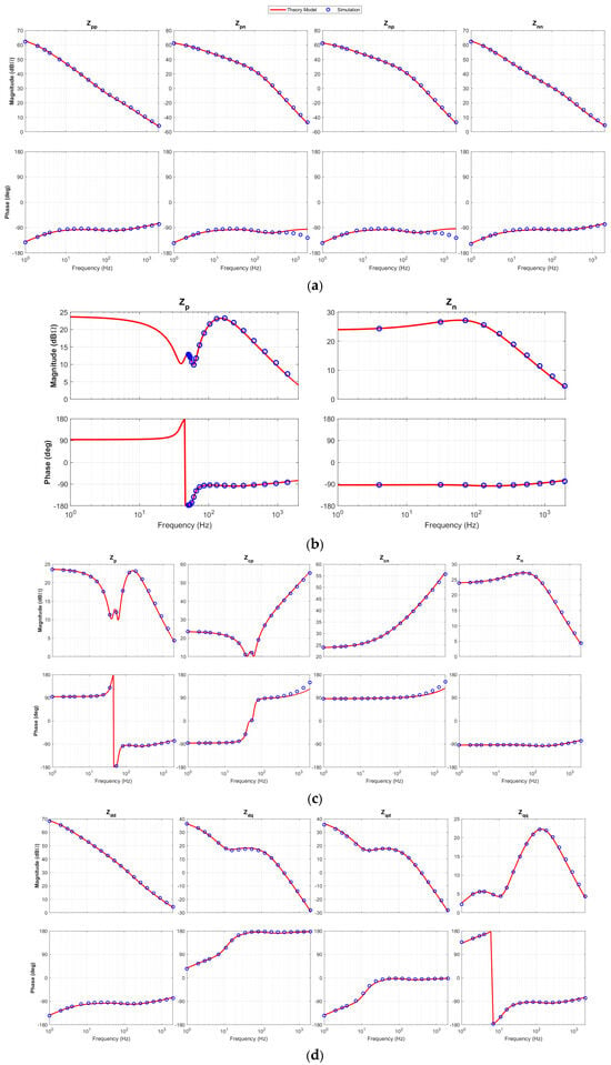
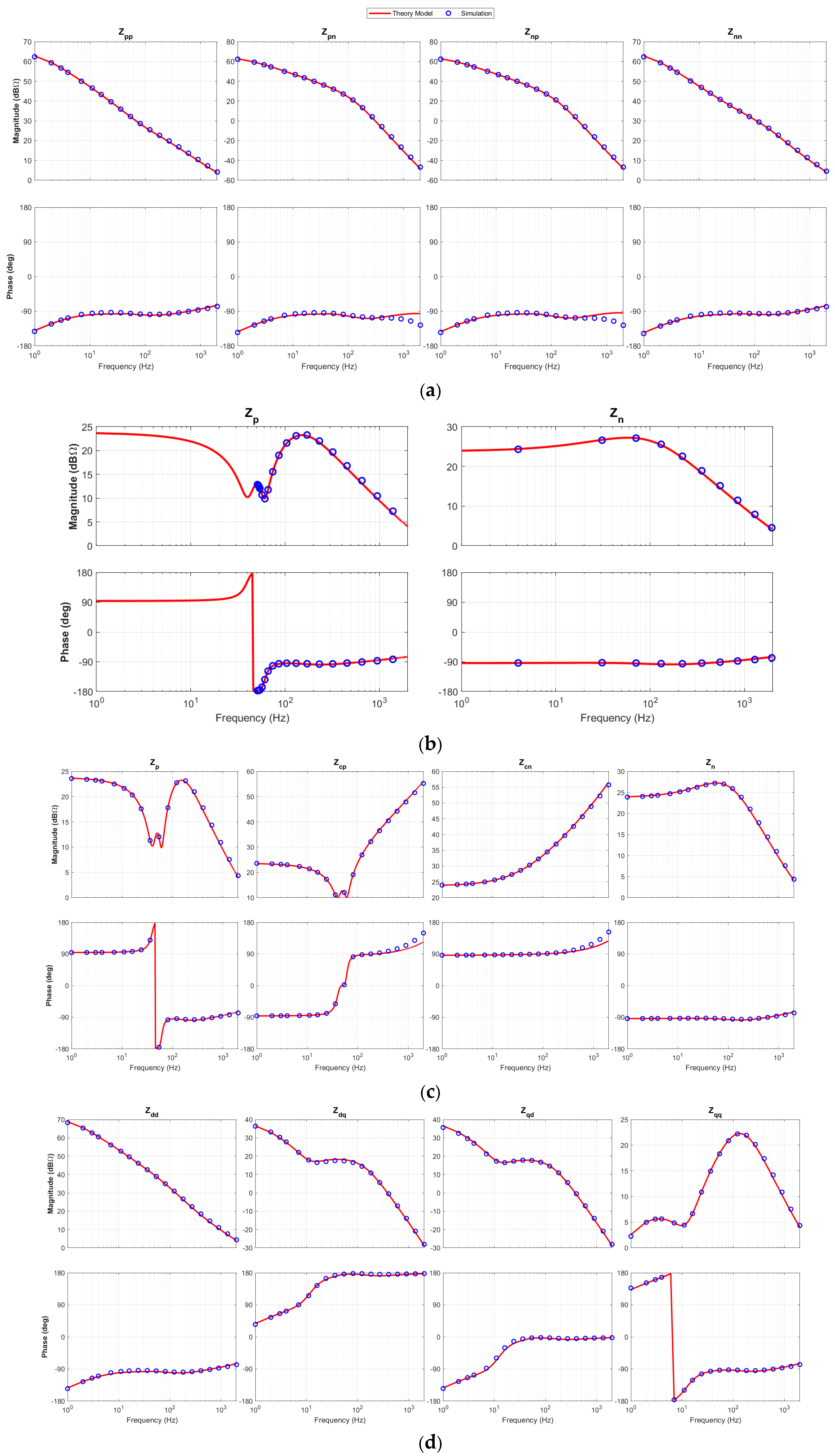
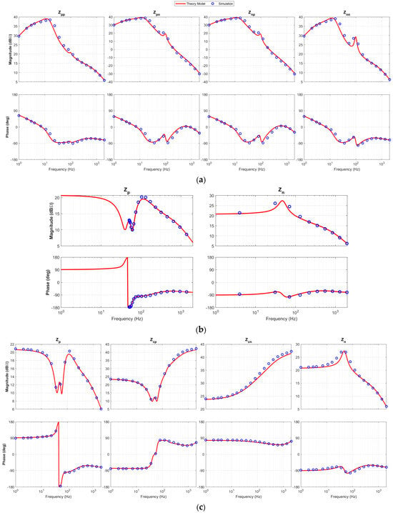
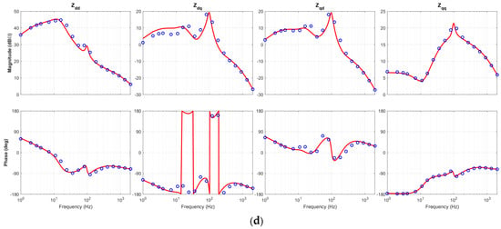
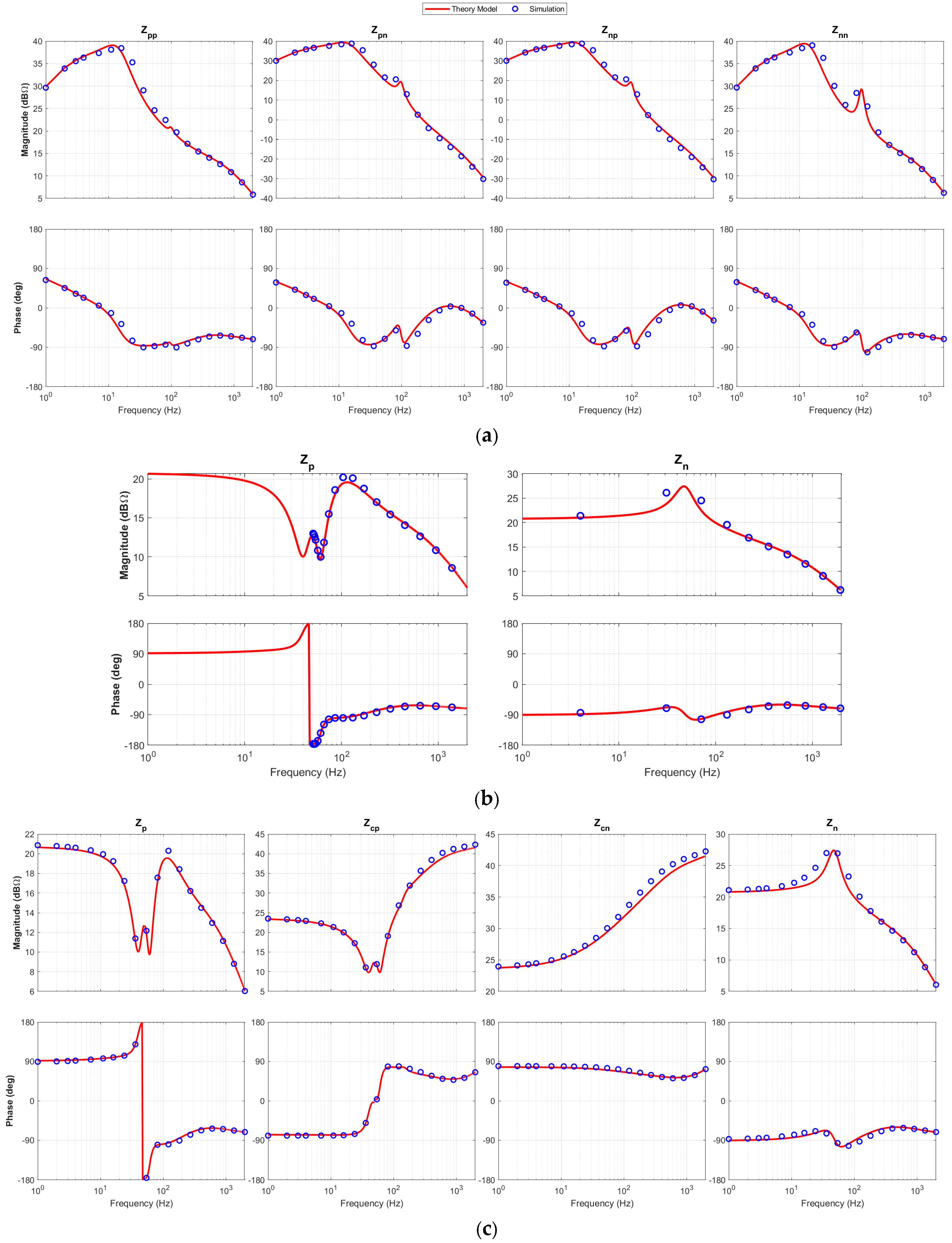
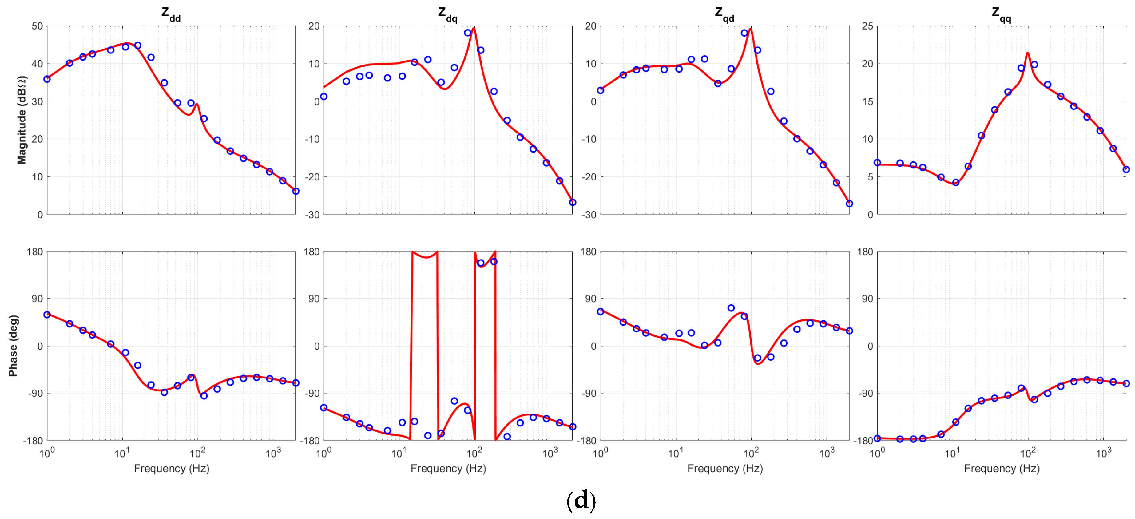
The theoretical model is validated by simulations in MATLAB/Simulink (R2023b Version and R2024a Version). The complete Simulink model is shown in Figure 3. The simulation reproduces the structure of Figure 2: a programmable three-phase source represents the grid, the LCL filter and the three-level bridge are modeled with the parameters of Table 2, and the current controller, capacitor-current active damping, PLL, PCC voltage feedforward and power loop are implemented as in Section 2 with the sampling and switching frequencies of Table 2. The main blocks are the grid source, the LCL filter, the bridge with PWM, the dq current controller with active damping, the SRF-PLL, the voltage-feedforward path, the power-loop controller, the perturbation source and the FFT-based measurement block. In this case, the power loop is disabled, so that the LCL filter, the inverter-side current control, the active damping, the PLL and the PCC voltage feedforward are validated in isolation. Positive- and negative-sequence voltage perturbations are injected at the PCC, the resulting current responses are recorded, and the parameters of the 215 kW industrial product are used. In Figure 4, the red lines are the predicted impedances and the blue dots are the simulated impedances over the scanned frequency range; panels (a)–(d) show the modified sequence impedance, the accurate SISO impedance, the coupled sequence impedance and the dq impedance, respectively.

Figure 3. Simulink model of the grid-connected inverter.

Figure 4. Impedance validation without power loop: (a) modified sequence impedance; (b) accurate SISO impedance; (c) coupled sequence impedance; (d) dq impedance.

8.2. Verification with Power Loop

In this case, the power loop is enabled but the active power feedforward is disabled. The power loop introduces additional dynamics that reshape the impedance characteristics, particularly at low frequencies where the power control bandwidth is dominant. Figure 5 shows the modified sequence impedance with the power-loop effects. As in Figure 4, the red lines are the predicted impedances and the blue dots the simulated ones, and panels (a)–(d) show the modified sequence impedance, the accurate SISO impedance, the coupled sequence impedance and the dq impedance. The agreement between model and simulation remains good, which validates the power-loop modeling.

Figure 5. Impedance validation with power loop but without feedforward: (a) modified sequence impedance; (b) accurate SISO impedance; (c) coupled sequence impedance; (d) dq impedance.

The agreement is quantified as follows. Over the scanned frequency range, which includes the LCL resonance and the band in which the PLL dominates, the maximum relative deviation between the predicted and the simulated impedance magnitudes is below 5%, and the phase curves coincide except in the immediate vicinity of the LCL resonance, where the phase changes steeply and the comparison is most sensitive to the filter parameters. The residual differences are not further corrected, because they originate from the simplifications of small-signal modeling and from practical effects: the small-signal model neglects the second-order terms, and the non-linear switching process appears only as background noise; in practice, the discretization of the controller and the non-linear behavior of the filter components introduce additional errors. Since these practical errors dominate the residual difference, there is no need to correct the small modeling error, and a loop-by-loop decomposition of the error is therefore also unnecessary.

9. Experimental Verification and Stability Enhancement

9.1. Stability Analysis for Different PLL Bandwidths and Measurement Setup

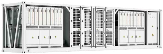
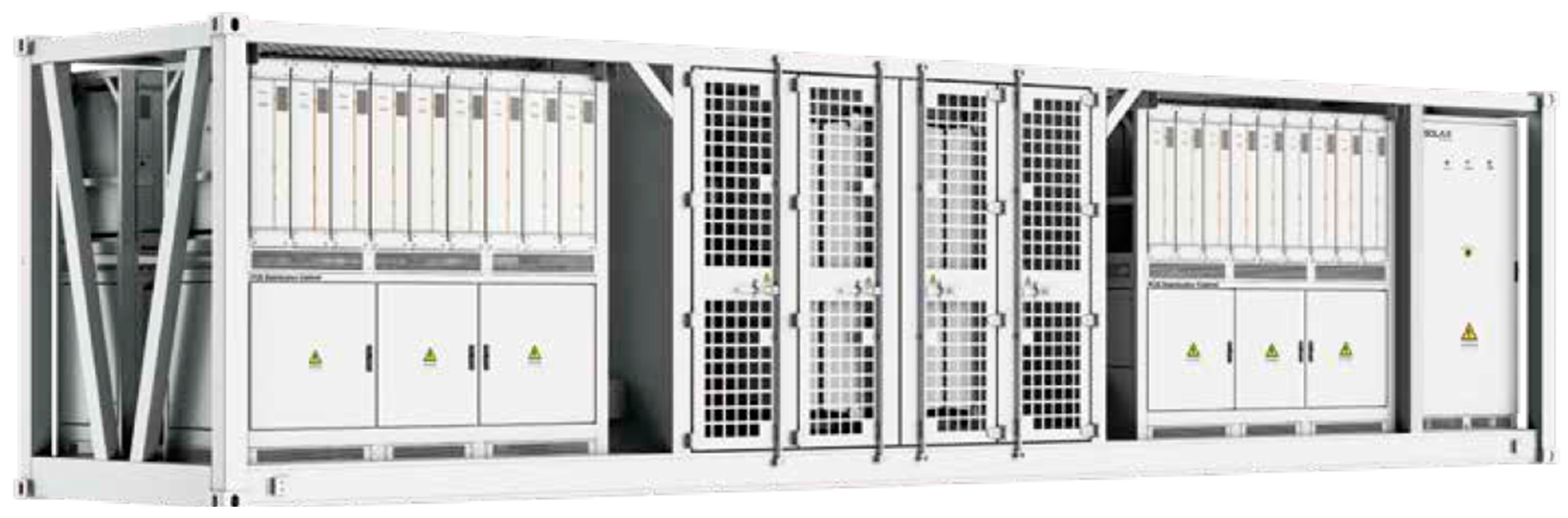
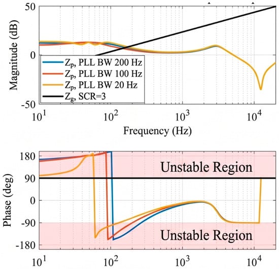
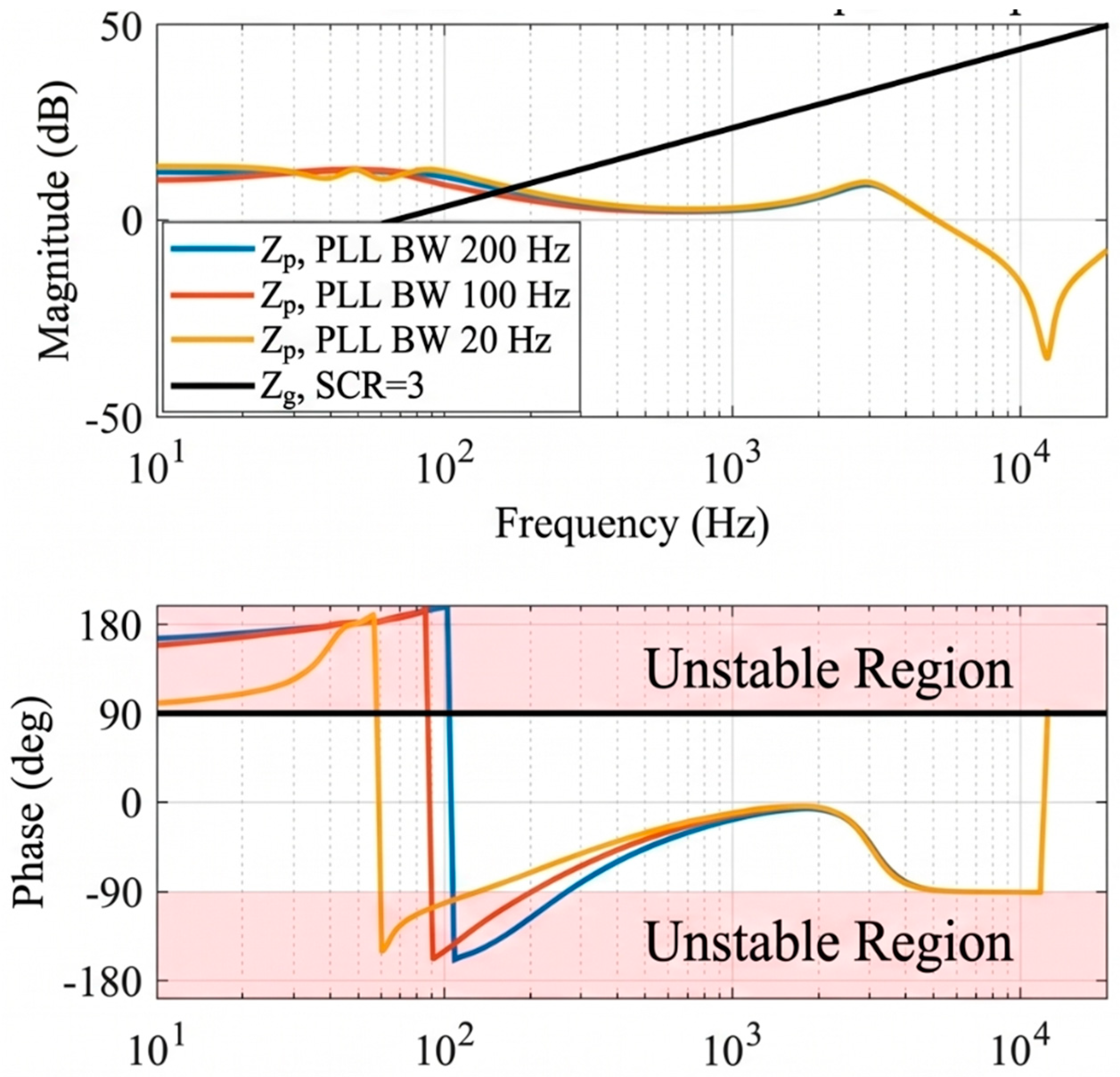
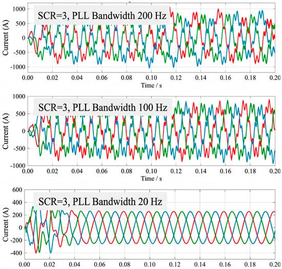
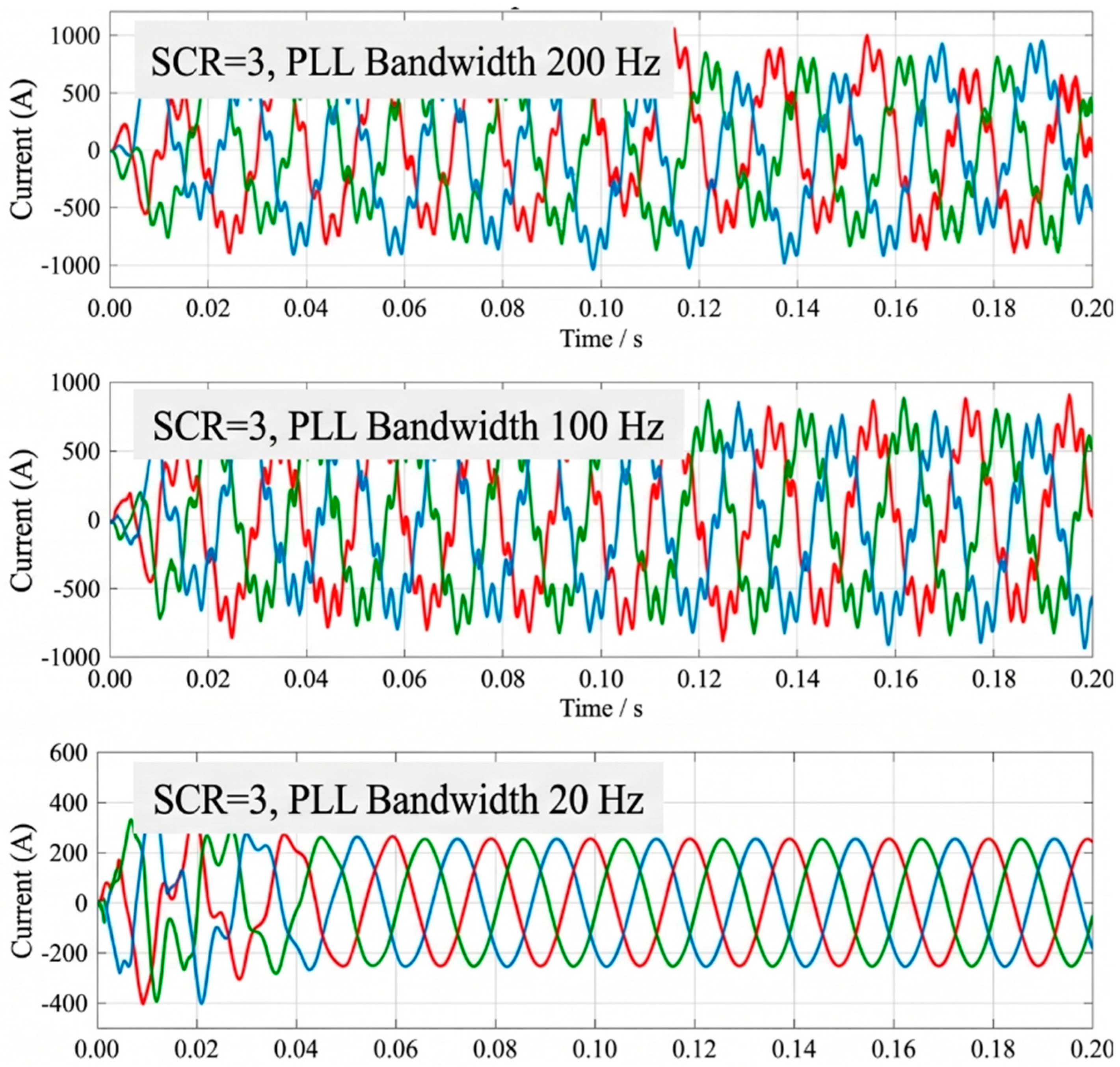
The proposed impedance model is experimentally validated on a 215 kW, 690 V three-phase grid-connected inverter product with an LCL filter, as shown in Figure 6. The prototype is a commercial product, so its detailed component breakdown cannot be disclosed; the electrical parameters that can be released are listed in Table 2. A programmable grid simulator emulates weak-grid conditions by varying the equivalent grid inductance Lg [29]. Three PLL bandwidth settings are tested: 20 Hz, 100 Hz and 200 Hz. Figure 7 shows the measured coupled sequence impedance magnitude and phase under a weak-grid condition; the results confirm that a wider PLL bandwidth reduces the phase margin, as predicted theoretically. Figure 8 presents the corresponding steady-state three-phase current waveforms: with a narrow PLL bandwidth, the currents remain sinusoidal, whereas a wide PLL bandwidth produces low-frequency oscillations that indicate the onset of instability. Table 5 summarizes the quantified stability margins. At a short-circuit ratio of 3, the phase margin falls from 12° to −25° and then to −45° as the PLL bandwidth increases from 20 Hz to 200 Hz, which confirms that a wide PLL bandwidth progressively erodes the stability margin of the inverter in a weak grid.

Figure 6. Experimental prototype.

Figure 7. Impedance analysis under different PLL bandwidths.

Figure 8. Three-phase current under different PLL bandwidths.

Table 5. Stability margins for different PLL bandwidths.

PLL Bandwidth	20 Hz	100 Hz	200 Hz
Phase Margin at SCR = 3	12°	−25°	−45°
SCR for Critical Stability	1.75	4.64	7.62

The stability margin is evaluated from the ratio of the grid impedance to the inverter impedance, L(s) = Z_g(s)/Z_p(s). The system is stable if the Nyquist plot of L(s) does not encircle the point (−1, j0); in the Bode form used here, the phase margin is PM = 180° + ∠L(jω_c), where ω_c is a frequency at which |L(jω_c)| = 1. When several 0 dB crossings occur, the smallest phase margin over all crossings in the scanned band is reported. The critical SCR is the value at which this minimum margin becomes zero: the grid inductance is increased in steps, the impedance scan is repeated, and the SCR at which the phase margin crosses zero is recorded. This is the procedure used to obtain the margins in Table 5 and the critical ratios in Table 5 and Table 6.

Table 6. Stability improvement with lead compensation.

Metric	Without Compensation	With Compensation
Phase Margin at SCR = 3	12°	40°
SCR for Critical Stability	1.54	1.43

9.2. Stability Improvement with Leading Compensation

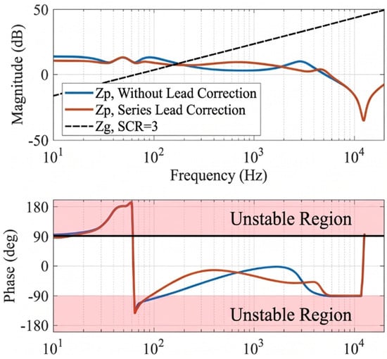
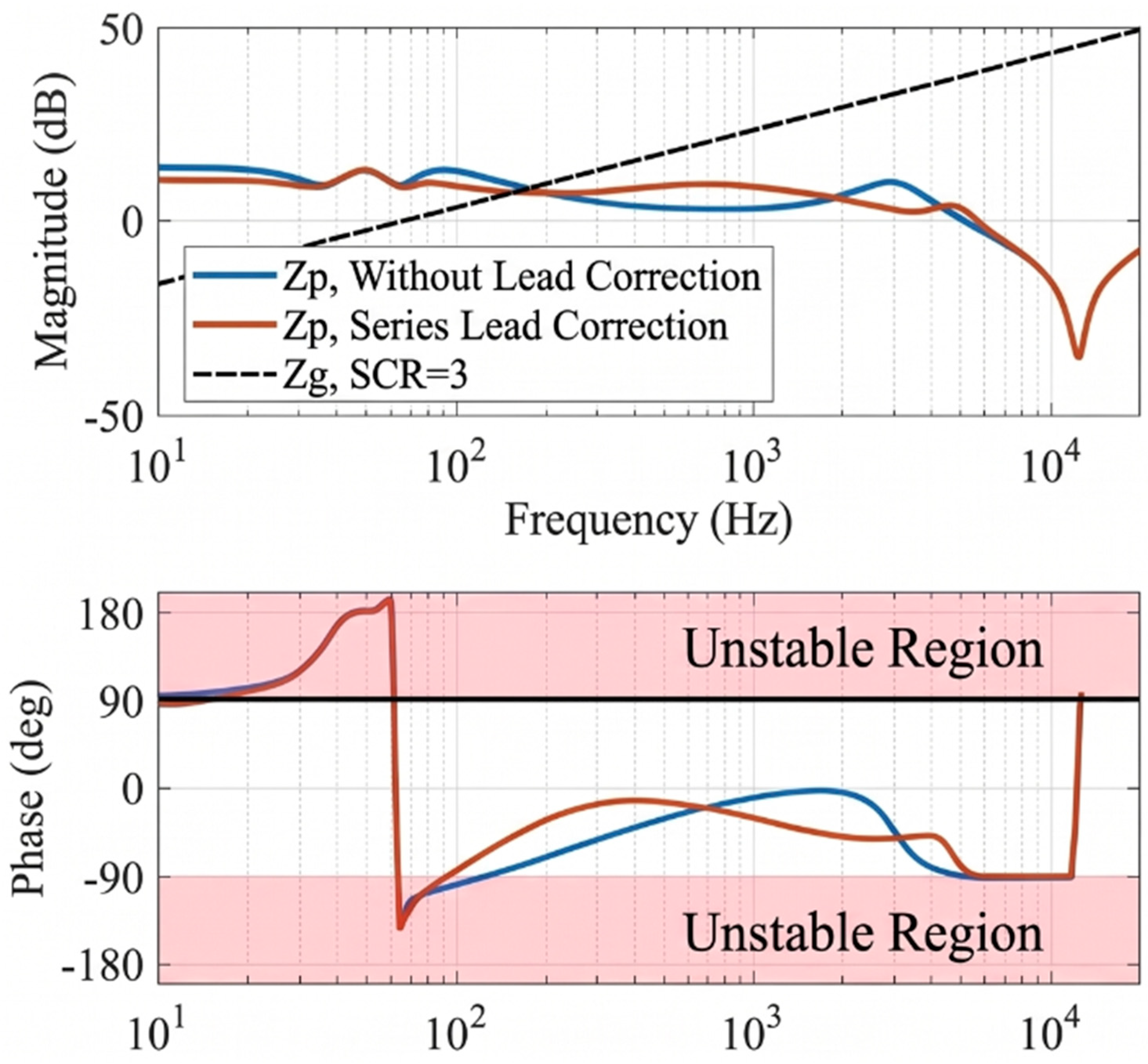
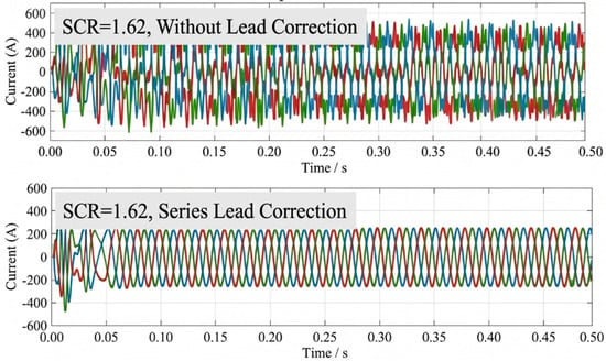
To improve stability under weak-grid conditions with a wide PLL bandwidth, a first-order lead compensator Glead(s) = (1 + s/ω_z)/(1 + s/ω_p), with ω_z ≈ 586 rad/s (93 Hz) and ω_p ≈ 2695 rad/s (429 Hz), is inserted in series with the current controller; these values correspond to a center frequency of 200 Hz and a maximum lead of 40°, and the PI parameters were retuned accordingly. Comparable admittance-reshaping approaches have been reported for LCL-type converters in weak grids [30,31]. Figure 9 compares the measured impedance with and without compensation under the same weak-grid condition. The compensated phase curve is shifted upward by about 26° in the critical band, which restores an adequate phase margin. Figure 10 shows the corresponding three-phase current waveforms: without compensation, sustained oscillations are visible, whereas with the lead compensator the oscillations are fully suppressed and sinusoidal currents are recovered at rated power. Table 6 quantifies the improvement: at a short-circuit ratio of 3 the phase margin rises from 12° to 40°, and the critical short-circuit ratio decreases from 1.54 to 1.43, i.e., stable operation is extended to a weaker grid. The lowest SCR is found by varying the grid impedance line and identifying the SCR at which the phase margin becomes zero. This confirms the validity of the impedance-based compensation design.

Figure 9. Impedance analysis with and without lead compensation.

Figure 10. Three-phase current with and without lead compensation.

10. Conclusions

This paper has addressed the impedance-based stability analysis of grid-connected LCL inverters whose complete industrial control structure is retained. The converter is described by a complex-vector dq-frame model, and the resulting sequence impedances are available in closed form in both regimes, f₁ < f_c and f₁ > f_c, without the multi-frequency algebraic equations that complex harmonic linearization would require. The sequence-domain definition itself is not assumed: it is obtained twice, once in the stationary alpha–beta frame and once through symmetrical components, and the two routes give the same expression for a converter that keeps the PLL, the active damping, the PCC voltage feedforward and the outer power loop.

Simulations and measurements were both used for validation. For the 215 kW, 690 V product, the measured impedances follow the predicted ones over the frequency range of interest, and the PLL bandwidth is identified as the dominant factor for the stability margin in a weak grid: at a short-circuit ratio of 3, the measured phase margin falls from 12° to −45° when the PLL bandwidth is increased from 20 Hz to 200 Hz. A first-order lead compensator designed from the impedance model raised the phase margin from 12° to 40° at the same operating point and extended stable operation to weaker grids, which shows that the model can be used for controller design and not only for analysis.

The main limitations of this study are that the small-signal model still contains a modeling error because the second-order terms are neglected and a first-order Taylor expansion is used, that the equivalence between the dq-frame and the sequence-domain impedances is established under balanced small-signal conditions, and that the experimental verification refers to a single industrial product. Unbalanced grid conditions, grid-forming control and multi-inverter systems are therefore left for future work.

References

- Liserre, M.; Blaabjerg, F.; Hansen, S. Design and Control of an LCL-Filter-Based Three-Phase Active Rectifier. IEEE Trans. Ind. Appl. 2005, 41, 1281–1291. [Google Scholar] [CrossRef] [Scilit]
- Dannehl, J.; Fuchs, F.W.; Hansen, S.; Thøgersen, P.B. Investigation of Active Damping Approaches for PI-Based Current Control of Grid-Connected PWM Converters with LCL Filters. IEEE Trans. Ind. Appl. 2010, 46, 1509–1517. [Google Scholar] [CrossRef] [Scilit]
- Liserre, M.; Teodorescu, R.; Blaabjerg, F. Stability of Photovoltaic and Wind Turbine Grid-Connected Inverters for a Large Set of Grid Impedance Values. IEEE Trans. Power Electron. 2006, 21, 263–272. [Google Scholar] [CrossRef] [Scilit]
- Turner, R.; Walton, S.; Duke, R. Stability and Bandwidth Implications of Digitally Controlled Grid-Connected Parallel Inverters. IEEE Trans. Ind. Electron. 2010, 57, 3685–3694. [Google Scholar] [CrossRef] [Scilit]
- Sun, J. Impedance-Based Stability Criterion for Grid-Connected Inverters. IEEE Trans. Power Electron. 2011, 26, 3075–3078. [Google Scholar] [CrossRef] [Scilit]
- Harnefors, L.; Bongiorno, M.; Lundberg, S. Input-Admittance Calculation and Shaping for Controlled Voltage-Source Converters. IEEE Trans. Ind. Electron. 2007, 54, 3323–3334. [Google Scholar] [CrossRef] [Scilit]
- Wen, B.; Boroyevich, D.; Burgos, R.; Mattavelli, P.; Shen, Z. Analysis of D-Q Small-Signal Impedance of Grid-Tied Inverters. IEEE Trans. Power Electron. 2016, 31, 675–687. [Google Scholar] [CrossRef] [Scilit]
- Bakhshizadeh, M.K.; Wang, X.; Blaabjerg, F.; Hjerrild, J.; Kocewiak, Ł.; Bak, C.L.; Hesselbæk, B. Couplings in Phase Domain Impedance Modelling of Grid-Connected Converters. IEEE Trans. Power Electron. 2016, 31, 6792–6796. [Google Scholar] [CrossRef] [Scilit]
- Wang, X.; Blaabjerg, F. Harmonic Stability in Power Electronic-Based Power Systems: Concept, Modeling, and Analysis. IEEE Trans. Smart Grid 2019, 10, 2858–2870. [Google Scholar] [CrossRef] [Scilit]
- Rygg, A.; Molinas, M.; Zhang, C.; Cai, X. A Modified Sequence-Domain Impedance Definition and Its Equivalence to the dq-Domain Impedance Definition for the Stability Analysis of AC Power Electronic Systems. IEEE J. Emerg. Sel. Top. Power Electron. 2016, 4, 1383–1396. [Google Scholar] [CrossRef] [Scilit]
- Parker, S.G.; McGrath, B.P.; Holmes, D.G. Regions of Active Damping Control for LCL Filters. IEEE Trans. Ind. Appl. 2014, 50, 424–432. [Google Scholar] [CrossRef] [Scilit]
- Sun, J. Small-Signal Methods for AC Distributed Power Systems—A Review. IEEE Trans. Power Electron. 2009, 24, 2545–2554. [Google Scholar] [CrossRef] [Scilit]
- Wu, W.; Zhou, L.; Chen, Y.; Luo, A.; Dong, Y.; Zhou, X.; Xu, Q.; Yang, L. Sequence-Impedance-Based Stability Comparison Between VSGs and Traditional Grid-Connected Inverters. IEEE Trans. Power Electron. 2019, 34, 46–52. [Google Scholar] [CrossRef] [Scilit]
- Cao, W.; Ma, Y.; Wang, F. Sequence-Impedance-Based Harmonic Stability Analysis and Controller Parameter Design of Three-Phase Inverter-Based Multibus AC Power Systems. IEEE Trans. Power Electron. 2017, 32, 7674–7693. [Google Scholar] [CrossRef] [Scilit]
- Sun, J.; Liu, H. Sequence Impedance Modeling of Modular Multilevel Converters. IEEE J. Emerg. Sel. Top. Power Electron. 2017, 5, 1427–1443. [Google Scholar] [CrossRef] [Scilit]
- Rygg, A.; Molinas, M.; Zhang, C.; Cai, X. On the Equivalence and Impact on Stability of Impedance Modeling of Power Electronic Converters in Different Domains. IEEE J. Emerg. Sel. Top. Power Electron. 2017, 5, 1444–1454. [Google Scholar] [CrossRef] [Scilit]
- Zhang, C.; Cai, X.; Rygg, A.; Molinas, M. Sequence Domain SISO Equivalent Models of a Grid-Tied Voltage Source Converter System for Small-Signal Stability Analysis. IEEE Trans. Energy Convers. 2018, 33, 741–749. [Google Scholar] [CrossRef] [Scilit]
- Meng, L.; Karaagac, U.; Jacobs, K. A New Sequence-Domain EMT-Level Multi-Input Multi-Output Frequency Scanning Method for Inverter-Based Resources. Electr. Power Syst. Res. 2023, 220, 109312. [Google Scholar] [CrossRef] [Scilit]
- Shah, S.; Koralewicz, P.; Gevorgian, V.; Wallen, R. Sequence Impedance Measurement of Utility-Scale Wind Turbines and Inverters: Reference Frame, Frequency Coupling, and MIMO/SISO Forms. IEEE Trans. Energy Convers. 2022, 37, 75–86. [Google Scholar] [CrossRef] [Scilit]
- Cespedes, M.; Sun, J. Impedance Modeling and Analysis of Grid-Connected Voltage-Source Converters. IEEE Trans. Power Electron. 2014, 29, 1254–1261. [Google Scholar] [CrossRef] [Scilit]
- Liu, G.; Liu, K.; Yao, Y.; Liu, C.; Wang, L.; Wang, X.; Tao, Y. Impedance Modelling and Stability Analysis of Grid-Connected Inverters with Power Loop and Feedforward Control. In Proceedings of the 2026 5th International Conference on Green Energy and Power Systems (ICGEPS), Hangzhou, China, 17–19 April 2026; pp. 725–730. [Google Scholar] [CrossRef] [Scilit]
- Kim, S.-D.; Tran, T.V.; Yoon, S.-J.; Kim, K.-H. Current Controller Design of Grid-Connected Inverter with Incomplete Observation Considering L-/LC-Type Grid Impedance. Energies 2024, 17, 1855. [Google Scholar] [CrossRef] [Scilit]
- Dong, D.; Wen, B.; Boroyevich, D.; Mattavelli, P.; Xue, Y. Analysis of Phase-Locked Loop Low-Frequency Stability in Three-Phase Grid-Connected Power Converters Considering Impedance Interactions. IEEE Trans. Ind. Electron. 2015, 62, 310–321. [Google Scholar] [CrossRef] [Scilit]
- Golestan, S.; Guerrero, J.M.; Vasquez, J.C. Three-Phase PLLs: A Review of Recent Advances. IEEE Trans. Power Electron. 2017, 32, 1894–1907. [Google Scholar] [CrossRef] [Scilit]
- Yang, D.; Ruan, X.; Wu, H. Impedance Shaping of the Grid-Connected Inverter with LCL Filter to Improve Its Adaptability to the Weak Grid Condition. IEEE Trans. Power Electron. 2014, 29, 5795–5805. [Google Scholar] [CrossRef] [Scilit]
- Blaabjerg, F.; Teodorescu, R.; Liserre, M.; Timbus, A.V. Overview of Control and Grid Synchronization for Distributed Power Generation Systems. IEEE Trans. Ind. Electron. 2006, 53, 1398–1409. [Google Scholar] [CrossRef] [Scilit]
- Wu, H.; Ruan, X.; Yang, D.; Chen, X.; Zhao, W.; Lv, Z.; Zhong, Q.-C. Small-Signal Modeling and Parameters Design for Virtual Synchronous Generators. IEEE Trans. Ind. Electron. 2016, 63, 4292–4303. [Google Scholar] [CrossRef] [Scilit]
- Wen, B.; Burgos, R.; Boroyevich, D.; Mattavelli, P.; Shen, Z. AC Stability Analysis and dq Frame Impedance Specifications in Power-Electronics-Based Distributed Power Systems. IEEE J. Emerg. Sel. Top. Power Electron. 2017, 5, 1455–1465. [Google Scholar] [CrossRef] [Scilit]
- Feng, G.; Ye, Z.; Xia, Y.; Huang, L.; Wang, Z. Impedance Modeling and Stability Analysis of Three-Phase Four-Wire Inverter with Grid-Connected Operation. Energies 2022, 15, 2754. [Google Scholar] [CrossRef] [Scilit]
- Jin, J.; Tang, X.; Zhou, Z.; Tang, K.; Wang, J. Admittance-Reshaping Method for LCL-Type Grid-Connected Converters Under Weak-Grid Conditions and Background Harmonic Disturbances. Energies 2026, 19, 2884. [Google Scholar] [CrossRef] [Scilit]
- Liu, L.; Wang, K.; Peng, F.; Tian, Y.; Wang, Y. Dynamic Grid Voltage-Based Impedance-Reshaped Control for the Stability Enhancement of Grid-Connected DC/AC Converter System under Bidirectional Power Flow. Energies 2022, 15, 7269. [Google Scholar] [CrossRef] [Scilit]
Disclaimer/Publisher’s Note: The statements, opinions and data contained in all publications are solely those of the individual author(s) and contributor(s) and not of MDPI and/or the editor(s). MDPI and/or the editor(s) disclaim responsibility for any injury to people or property resulting from any ideas, methods, instructions or products referred to in the content. |
© 2026 by the authors. Licensee MDPI, Basel, Switzerland. This article is an open access article distributed under the terms and conditions of the Creative Commons Attribution (CC BY) license.