Model-Based Positive Generation Gaps and Smart EV Charging Potential: A 2020–2025 Case Study of Photovoltaics, Wind Power, and Hydropower

Abstract

This study compares theoretical annual renewable generation with recorded grid injection from one Polish distribution system operator for 2020–2025. Across 1513 source-year records, the cumulative positive model–injection difference is 3148.304 GWh. Large sources contribute 96.00%, while wind contributes 92.75% under an assumed capacity factor of 0.24. An annual charging calculation uses a hypothetical fleet of 20,043 electric vehicles with a demand of 53.308 GWh/year. Assuming full eligibility of the positive difference and 90% conditional capture, large-source scenarios for 2025 cover 47.34%, 100.00% and 65.67% of demand for photovoltaics, wind and hydropower, respectively. At 10% eligibility, coverage falls to 4.75%, 91.12% and 6.57%. Scaling reference generation by ±20% gives positive differences of 1874.982–4429.287 GWh. In a sensitivity analysis, excluding nine implausible hydropower records reduces root mean square error from 3545.5 to 2078.4 MWh/(MW·year), without changing the positive total. These conditional accounting results identify priorities for data reconciliation and subsequent operational measurements. They do not measure curtailment or demonstrate temporal coincidence, network deliverability, realized charging potential or economic benefit.

1. Introduction

Increasing renewable generation makes flexible demand, storage, and network operation central to electricity-system integration. Bird et al. [1] review international wind and solar curtailment experience, Li et al. [2] examine renewable curtailment and avoidance with a Chinese case, and O’Shaughnessy et al. [3] focus on global PV curtailment trends. These studies establish curtailment as an operational and system-integration problem. The present study examines a related but distinct quantity: the difference between generation possible under stated regional reference conditions and electricity recorded as injected into the distribution grid. Its numerical value follows from paired model and DSO energy records; assigning its cause requires a separate analysis.

System-level studies provide a second perspective. Lund and Mathiesen [4] analyse a Danish renewable-energy system, while Denholm and Hand [5] address the flexibility and storage needed at high variable-renewable penetration. Victoria et al. [6] examine storage in a sector-coupled European system, and Brown et al. [7] study sector coupling together with transmission reinforcement. European feasibility and balancing are addressed by Zappa et al. [8], Rasmussen et al. [9], and Heide et al. [10]. These system-wide questions complement the present operator-record analysis, which retains regional assignment and separates technology and capacity effects within the supplied 2020–2025 dataset.

Papaefthymiou and Dragoon [11] and Lund et al. [12] frame the broader flexibility problem, while Peker et al. [13] consider transmission switching and storage. Laimon [14] discusses curtailment as a problem and an opportunity, and Soto-Valle and Usuba [15] provide a historical wind-curtailment case. These perspectives motivate the use of a DSO balance to identify and prioritize potential flexibility opportunities without assigning an operational cause from energy totals alone.

For PV, Huld and Amillo [16] explicitly consider irradiance, air temperature, wind speed, and solar spectrum over large geographical regions. De Soto et al. [17] address PV-array performance modelling and validation; Fahim et al. [18] review module models and parameter extraction. In comparison, the present PV calculation estimates regional reference yield from rated capacity, a location-selected irradiation profile, module geometry, and aggregate system losses. The distinction is methodological: a regional energy-balance model answers a different question from a detailed module-performance model. Rajesh and Mabel [19] provide the broader PV-system context, Jordan and Kurtz [20] address degradation, and Skoplaki and co-authors [21,22] address operating temperature. These effects delimit the interpretation of the simplified reference yield.

For wind energy, Carta et al. [23] review wind-speed distributions, Murthy and Rahi [24] review resource assessment, and Lydia et al. [25] and Bilendo et al. [26] review power-curve modelling. Saint-Drenan et al. [27] present a parametric power-curve model with environmental conditions. The present annual CF calculation is simpler and uses regional profiles for monthly allocation. Igliński et al. [28] provide Polish sector context, and Pryor and Barthelmie [29] discuss climatic influences; neither type of context turns a common CF into site-specific operating data.

For hydropower, Hamududu and Killingtveit [30], Wasti et al. [31], and Turner et al. [32] address climate-related changes at broad geographical or system scales. Klein and Fox [33] focus on small-hydropower performance and cost, while Kasperek [34] discusses development in Poland. Yüksel [35], Zarfl et al. [36], and Tahseen and Karney [37] address development or sustainability. The present comparison instead uses annual source records and a regional reference-energy balance. Sobik [38] gives a complementary Polish context for PV during summer peak demand.

Electric-vehicle integration is reviewed through modelling approaches by Richardson [39], through interaction with renewable generation by Mwasilu et al. [40], and through smart charging strategies by Sadeghian et al. [41]. Barman et al. [42] review charging approaches for renewable integration. The most directly related application studies have different objectives: Szinai et al. [43] examine charging management in relation to operating costs and renewable curtailment; Dixon et al. [44] address charging schedules, carbon emissions, and wind curtailment; Saadatmandi et al. [45] focus on PV curtailment. Here, charging is evaluated against a regional DSO potential–injection balance using a fixed vehicle fleet and explicit annual energy and power limits. Its demand-coverage percentages are therefore scenario results under the stated balance, rather than directly comparable curtailment-reduction percentages.

Lund and Kempton [46] consider V2G in renewable and transport integration; Kempton and Tomić [47] address its capacity and revenue fundamentals. Tan et al. [48] review V2G technology and optimization, Sovacool et al. [49] discuss its social research agenda, and Das et al. [50] review charging standards, infrastructure, and grid effects. Inci et al. [51] provide a broader grid-integration review, and Flasza and Matuszczyk [52] present a Polish electromobility/renewables perspective. Blumberg et al. [53] analyse future European electricity-system EV scenarios, while IRENA [54] and the US Department of Energy [55] provide smart-charging and vehicle–grid integration assessments. These works supply complementary context for the explicitly bounded annual EV calculation used here.

Three questions organize the analysis. First, how do positive reference-model–injection differences vary across technologies, years and source capacity classes? Second, how do reference assumptions and anomalous records affect signed balances and normalized diagnostics? Third, what conditional annual EV-demand coverage follows when a stated fraction of the positive difference is used as a hypothetical charging input?

The contribution is the integration of formal DSO regional assignment, three renewable technologies, six annual reporting periods, three capacity classes, and a constrained EV-use calculation in a common accounting framework. The study combines 1513 complete source-year records, positive and signed energy balances, capacity-normalized indicators, and 54 technology–year–capacity scenarios for a 30-model fleet. This empirical combination makes it possible to distinguish the sources that dominate total potential from those with the highest difference per unit of installed capacity. Table 1 compares the analytical scope of the principal references with the present study.

Table 1. Analytical scope of selected studies and their relation to the present regional DSO framework.

Topic	Principal References	Comparison and Contribution
Curtailment	Bird et al. [1]; Li et al. [2]; O’Shaughnessy et al. [3]	International experience, avoidance, and PV trends provide operational context. This study quantifies a paired source-year potential–injection gap and reports its signed and negative components.
System flexibility	Denholm and Hand [5]; Victoria et al. [6]; Brown et al. [7]	Storage, sector coupling, and transmission are system-level flexibility questions. The present contribution is a regional DSO record balance linked to a constrained EV-use scenario.
PV performance	Huld and Amillo [16]; De Soto et al. [17]; Fahim et al. [18]	Regional performance drivers, array-model validation, and parameter extraction motivate explicit model scope. Here, a location-selected profile, capacity, geometry, and aggregate losses define reference yield.
Wind modelling	Carta et al. [23]; Lydia et al. [25]; Saint-Drenan et al. [27]	Wind-speed distributions and power-curve models describe resource or turbine performance. Here, the reference CF setting is 0.24; normalized regional weights determine monthly allocation.
Hydropower	Hamududu and Killingtveit [30]; Klein and Fox [33]; Kasperek [34]	Climate effects, small-hydro performance/cost, and Polish development provide complementary scales. The present annual calculation uses capacity-class CF settings and regional seasonal profiles.
Smart charging	Szinai et al. [43]; Dixon et al. [44]; Saadatmandi et al. [45]	The cited applications address operating costs, emissions, and wind/PV curtailment. Here, annual fleet-demand coverage is evaluated from a multi-technology potential–injection resource with explicit charging limits.
V2G and EV scenarios	Lund and Kempton [46]; Kempton and Tomić [47]; Blumberg et al. [53]	Renewable integration, V2G capacity/revenue, and future European EV scenarios motivate flexibility assessment. Here, a fixed 20,043-vehicle fleet is evaluated under compatibility, SOC, participation, and cycle limits.
Present study	Regional DSO data, 2020–2025	A total of 1513 complete records; PV, WE, and HE; three capacity classes; positive and signed accounting; capacity exposure; and 54 annual EV-use scenarios within one explicitly specified annual accounting framework.

The framework addresses the joint reporting of annual reference-model differences, signed balances, capacity exposure and conditional EV-demand coverage for this operator dataset. Relative to the analytical scopes in Table 1, it distinguishes the technology dominating the absolute positive difference (WE, 92.75%) from the capacity class with the highest normalized intensity (small sources). These are dataset-specific accounting findings under stated reference assumptions. Retaining negative differences and testing eligibility fractions makes explicit why a positive model residual cannot be equated with recoverable curtailed energy. The integration of these accounting steps is the methodological contribution; it does not establish a new independently validated resource or dispatch model.

2. Materials and Methods

2.1. Study Design, Data Scope, and Representativeness

The annual renewable-energy records originate from the formal regional operating units of one Polish distribution system operator (DSO). Individual source information is anonymized, while the regional keys remain available for selecting the corresponding model parameters and profiles. The model documentation organizes the territory into 11 DSO areas. The annual tables use the regional codes OBB, OBD, OCZ, OGL, OJG, OKR, OLG, OOP, OTR, OWB, and OWR. Regional assignment is therefore an explicit input to the calculation. The study concerns the supplied DSO records and does not extrapolate their energy totals to all Polish distribution operators.

The analysis includes the source-year rows present in the supplied annual technology workbooks. No independently verified inventory was available to establish whether these files cover every eligible installation or whether reporting definitions remained unchanged across 2020–2025. The annual source roster is not constant, and installations cannot be linked by a stable identifier across years. Year-to-year differences can therefore reflect reporting coverage and roster composition as well as resource or operational changes. The files support a within-dataset comparison, not an estimate of coverage of the entire distribution territory.

The 18 annual technology workbooks contain 1539 source-year rows for 2020–2025. Twenty-six HE micro-source rows report zero energy and lack installed capacity; these rows cannot support the normalized comparison and are excluded. The analytical sample comprises 1513 complete records: 660 PV, 347 WE, and 506 HE. The unit of analysis is a source-year record, not a confirmed count of unique installations across the six-year period. The capacity classes are micro (up to 50 kW), small (above 50 kW and up to 500 kW), and large (above 500 kW). Each paired comparison retains the capacity, regional key, modelled energy, and recorded grid injection from the same annual source record.

Installed capacity was taken from each annual record. Annual tables therefore reflect changes in the roster and capacity represented in each year. Across multiple years, capacity is reported as exposure in MW·year, calculated as the sum of annual nameplate capacities. Exact commissioning and retirement dates were unavailable. A source commissioned part-way through a year may therefore have a lower metered yield per MW than a full-year source; no within-year correction was imputed.

The regional keys serve different roles in the three model branches. PV locations select a radiation zone or DSO-area productivity profile before the energy calculation. Wind locations select one of 11 DSO seasonal profiles, which distribute an annual CF-based total. Hydro locations select a regional profile derived from reference-gauge flows; the documented model also distinguishes physical and scenario branches. Formal operating areas are the spatial indexing framework. Their use does not require that all sites within an area have identical local weather or hydraulic conditions.

Regional monthly profiles are appropriate inputs for the stated regional reference-balance and seasonal-allocation calculations. Their assignment does not itself demonstrate measured site-specific accuracy. When annual observations are distributed using the same normalized profile as the model, the resulting monthly values are reconstructed allocations. The article’s reported generation gaps are calculated from the paired annual values, and no reconstructed monthly series is treated as an independent set of measured observations.

2.2. Photovoltaic Reference Model

The PV model estimates generation potential from rated capacity, the monthly profile selected for the source’s location, a tilt-and-azimuth correction, and an aggregate system performance ratio [16,17,19]. The documentation distinguishes a three-zone predictor from an 11-area DSO reconstruction/calibration branch. The spatial selection is made before energy is calculated; one universal national profile is not assigned to all sources. For source i and month m,

E_PV(i, m) = P(i) H(m) K_geo(i) PR_sys(i)

(1)

P(i) is rated capacity in kWp, H(m) is the location-selected reference-yield profile in equivalent reference hours, K_geo(i) is dimensionless and PR_sys(i) is the aggregate performance ratio. Irradiation in kWh/m² is divided by 1 kW/m² to obtain H(m), so Equation (1) gives kWh. The documented geometry rule is K_geo(i) = max{0.50, 1 − 0.00006[θ(i) − 35]² − 0.000022φ(i)²}, where θ is tilt in degrees and φ is azimuth in degrees relative to south. Its maximum is one at θ = 35° and φ = 0°. The coefficients and floor are empirical workbook assumptions, not independently validated site corrections. PR_sys = 1 − L_sys = 0.84 follows from the assumed aggregate loss fraction L_sys = 0.16. Temperature, shading, clipping, soiling, snow and outages are not separately resolved.

The annual PV model values are retained from the supplied annual workbooks. In 650 of the 660 records, modelled yield per unit of capacity equals 897.12, 948.36, or 996.24 MWh/MW, consistent with monthly irradiation sums of 1068, 1129, or 1186 kWh/m² and a 0.84 performance ratio at reference geometry. The remaining ten records retain their supplied model values rather than being silently reassigned to a profile.

For reproducibility, the applied monthly-profile sums must be distinguished from the predictor documentation’s alternative annual GHI labels of 980, 1030, and 1080 kWh/m². The documented predictor sums the monthly entries and does not normalize them to those labels. Accordingly, this article reproduces the supplied annual model-energy values; it does not substitute a different annual irradiation baseline. In the calibration branch, an annual observed total can be distributed according to the selected DSO profile, but fitting that total is calibration rather than independent validation of generation potential.

The monthly-profile sums and alternative annual GHI labels are inconsistent inputs in the supplied predictor documentation; the original provenance of that discrepancy is not established. For the 650 standard-yield records, substituting 980, 1030 and 1080 kWh/m² for 1068, 1129 and 1186 kWh/m², respectively, while retaining the ten non-standard records, reduces the cumulative PV positive gap from 70.083 to 59.795 GWh (14.68%). Thus, the choice materially affects the PV residual. The ten exceptional records contribute 0.136 GWh to the positive gap and are listed in Supplement S1. Several values are consistent with a capacity/model-value alignment issue, but the cause cannot be confirmed without the original calculation history. Their supplied values are retained and flagged. The annual assessment does not use reconstructed monthly outputs as observations. All ten flagged PV records remain in the baseline energy balances and in the normalized diagnostics. Supplement S1 reports their combined contribution to the positive difference; it does not report a PV diagnostic-exclusion experiment. No corrected measurements are imputed without source reconciliation.

2.3. Wind Energy Reference Model

Annual WE reference generation is P(i) × 8760 × CF in MWh when P(i) is in MW. All 347 supplied WE values reproduce CF = 0.24, equivalent to 2102.4 MWh/MW in the standard model year. Regional monthly weights only redistribute this total. The annual calculation includes neither site-specific wind resource nor turbine power curves [23,24,25,26,27]. The 0.24 setting is a scenario baseline, not a locally validated estimate. The unweighted mean metered yield is 647.6 MWh/MW, equivalent to approximately 0.074 of standard-year capacity, whereas the capacity-weighted large-source yield is about 1077 MWh/MW. These different averaging conventions should not be conflated. The 92.75% wind share of the positive gap is therefore strongly dependent on the CF = 0.24 assumption; without localized wind reanalysis, this share cannot be treated as a resource characteristic of the territory.

A wind-only diagnostic changes CF to 0.192 and 0.288 while retaining all PV and HE inputs. The WE positive gap becomes 1732.816 and 4110.603 GWh, and the all-technology total becomes 1961.176 and 4338.963 GWh, respectively. A wider exploratory stress test at CF = 0.12, 0.18 and 0.30 is reported in Supplement S2. These are deterministic assumptions, not a meteorologically justified uncertainty interval. Low metered yields may reflect partial-year operation, meter boundaries, capacity alignment, reporting coverage, resource mismatch or operating constraints. The files do not separate these causes. Localized wind-resource reanalysis has not been implemented: matching reanalysis to sites would require verified site locations, hub heights, turbine curves and operating periods. The uniform-CF results therefore remain theoretical benchmarks, and the 92.75% share is conditional on that baseline. The annual CF comparison is retained only as a transparent benchmark. It cannot determine regional available wind generation or substantiate recoverable curtailment, and sensitivity testing does not fulfil the requested localized resource reconstruction.

2.4. Hydropower Reference Model

The supplied HE annual model values reproduce a capacity-factor rule: P(i) × 8760 × CF, with CF = 0.33 below 0.1 MW, 0.38 from 0.1 to 1 MW, 0.40 from 1 to 10 MW, and 0.35 above 10 MW. These settings are inferred from the applied workbook values at their reported precision. An independent hydraulic or empirical justification for these particular capacity-class settings is not documented. The separate model documentation also describes a physical flow–head–efficiency branch and technology-based catalogue settings; those should not be presented as evidence validating the capacity-class rule actually used here [30,31,33,35]. The annual HE calculation is therefore a reference scenario. The capacity-class coefficients are used to reproduce the supplied reference series; they are not estimated from this dataset or presented as validated hydrological parameters.

Nine HE records report annual injection above nameplate capacity multiplied by calendar-year hours. Their source values are retained for traceability, but they require operator reconciliation of capacity, energy units and meter boundaries. Removing them leaves 497 HE records and changes the signed HE balance from 151.387 to 152.431 GWh, the negative-difference magnitude from 6.889 to 5.846 GWh, MBE from 638.3 to 906.5, MAE from 2027.1 to 1807.2 and RMSE from 3545.5 to 2078.4 MWh/(MW·year). The HE positive gap remains 158.276 GWh and the all-technology positive total remains 3148.304 GWh. Supplement S3 gives the exclusion diagnostics and record locations.

The hydro regional profile is constructed by normalizing each reference gauge’s monthly flows and averaging the normalized profiles assigned to the region. It represents regional seasonality rather than the discharge at an individual plant cross-section. Both annual wind and hydro reference calculations retain the documented 8760 h standard year for all reporting years, including leap years. This convention is stated explicitly to preserve the supplied model totals. Table 2 summarizes the scope, assumptions and applicable interpretation of the three reference models.

Table 2. Scope, assumptions, and applicable interpretation of the reference generation models.

Technology	Reference Calculation	Factors Included	Major Factors Not Resolved	Applicable Interpretation
PV	Monthly P × H × Kgeo × PRsys	Regional solar profile, capacity, geometry, and system losses	Site weather, temperature, shading, clipping, and outages	Regional reference yield; calibrated monthly series are reconstructions
WE	Annual P × 8760 × CF; CF = 0.24 in annual records	Capacity, CF, and normalized DSO monthly weights	Wind speed, turbine curve, wakes, icing, and source availability	Annual reference level and regional seasonal allocation
HE	Annual P × 8760 × capacity class CF in annual records	Capacity, CF settings, and regional water profile	Site hydraulics and dispatch for annual scenario records	Annual scenario potential; documented physical branch is separate

The different equations reflect the inputs available in each branch. PV uses an irradiation-based yield and explicit geometry/loss factors. WE and HE use annual capacity-factor settings because site-specific aerodynamic or hydraulic inputs are not supplied for the annual comparison. This difference is a limitation of model detail and validation, not evidence that the three branches have comparable predictive accuracy.

2.5. Calculation Boundary and Positive Model-Balance Gap

E_model is the energy that the technology-specific mathematical model assigns to the source under its stated capacity, regional resource, and operating assumptions. E_meter is the energy reported in the paired Excel record as introduced into the distribution grid. The calculation therefore compares modelled generation potential with recorded grid injection, rather than with a second series of modelled values. Both inputs are annual energies in MWh before aggregation and conversion to GWh. Because gross generation and grid injection can have different boundaries, their difference can also include own consumption and internal losses. For each record i, Equations (2) and (3) define the signed difference and its positive part.

ΔE(i) = E_model(i) − E_meter(i)

(2)

ΔE⁺(i) = max{0, E_model(i) − E_meter(i)}

(3)

Equation (3) measures the positive part of a statistical reference-model residual, not a measured physical surplus. Summation before truncation and truncation before summation answer different questions. With U = Σmax{E_meter(i) − E_model(i), 0}, ΣΔE⁺(i) = ΣΔE(i) + U. Both the signed net difference and U are retained. A positive residual at one record and a negative residual elsewhere can offset in the signed annual accounting, but neither establishes simultaneous surplus, load or transferable energy on adjacent feeders.

For the charging screen, an additional eligibility fraction f between zero and one is applied to the positive residual before the capture coefficient α. Here, f represents the hypothetical share attributable to energy that could be made available, whereas α represents conditional capture of that eligible share under unresolved access and timing effects. Neither is estimated from curtailment logs. The baseline f = 1 is an optimistic accounting scenario, not an estimate of recoverability. Values f = 0, 0.10, 0.25, 0.50 and 1 are tested separately in Supplement S4. The ±20% generation test changes the reference residual and cannot substitute for this eligibility test.

The unit of analysis is a source-year record, not a confirmed installation. Exact commissioning and retirement dates were unavailable, so a source active for only part of a year can show a lower metered yield per MW without any operator constraint. Own consumption, internal losses and the precise meter boundary are not separated in the released files. The cumulative positive gap of 3148.304 GWh is the sum of positive record-level differences under the stated models. It is not energy shown to be recoverable.

2.6. Normalized Indicators

Three complementary indicators were used for group g. Potential utilization was ΣE_meter/ΣE_model. The positive gap rate was ΣΔE+/ΣE_model. Positive-gap intensity was ΣΔE+/ΣC. In Equation (5), C(i) denotes nameplate-capacity exposure for source-year record i: rated capacity in MW multiplied by the one-year reporting interval, in MW·year. It corresponds to P(i) in the reference models after unit conversion (PV capacity is expressed in kWp in Equation (1), whereas WE/HE capacity is expressed in MW). Summing C(i) over records gives the group’s capacity exposure; it does not correct for partial-year operation.

$$R_{\mathrm{gap}}(g)={\displaystyle \frac{{\sum }_{i\in g}{\Delta E}^{+}(i)}{{\sum }_{i\in g}{E}_{\mathrm{model}}\left(i\right)}}$$

(4)

$$I_{\mathrm{gap}}(g)={\displaystyle \frac{{\sum }_{i\in g}{\Delta E}^{+}(i)}{{\sum }_{i\in g}C\left(i\right)}}$$

(5)

R_gap is reported as a percentage and I_gap in MWh/(MW·year) for multi-year aggregates. Where U(i) > 0, utilization and the positive gap rate are not exact complements because positive and negative record-level differences are summarized separately. Equations (4) and (5) define the gap rate and the gap intensity.

2.7. Calculation Verification and Yield-Difference Diagnostics

Calculation verification is distinguished from independent empirical validation. Verification checks record completeness, MW/kW and MWh/kWh conversions, capacity classes, annual model rules, signed differences, record-level positive-part aggregation, and agreement between technology, class, and annual totals. The wind and hydro annual values are reproducible with the CF rules described above. A reconstructed monthly series that is calibrated to the same observed annual total does not provide an independent validation sample. Independent validation of generation potential would require available-production observations or production records with known resource and operating conditions; grid injection alone does not supply that common measurement boundary.

For descriptive diagnostics, each annual energy is divided by its source capacity. Let d(i) = [E_model(i) − E_meter(i)]/C(i), and let n be the number of complete records. MBE = Σd(i)/n, MAE = Σ|d(i)|/n and RMSE = [Σd(i)²/n]½. The normalized MAE and RMSE divide these values by the unweighted mean metered yield and multiply by 100. These are unweighted record-level difference metrics in MWh/(MW·year); they should not be compared directly with aggregate injection in GWh. They describe model-to-injection disagreement, not independently validated forecast accuracy. Different measurement boundaries and erroneous records can both contribute.

A capacity–energy plausibility check additionally identifies nine HE records whose reported annual grid injection exceeds nameplate capacity multiplied by the hours in that calendar year. These source values are retained and flagged for reconciliation of capacity, units, or reporting boundary. All nine have negative potential–injection differences. Excluding them in a sensitivity check therefore leaves the cumulative positive gap of 3148.304 GWh unchanged, although it changes signed totals and HE difference diagnostics.

2.8. Reference EV Fleet and Annual Demand

The EV calculation used the same fixed reference fleet in every renewable-energy scenario. It contained 30 vehicle models with an assigned count of 20,043 vehicles: 26 BEV models and four PHEV models. Model counts, energy consumption, battery capacity, AC charging power, and V2G scenario flags were taken from the supplied vehicle dataset, compiled from CEPiK and vehicle-specification sources [56,57]. The reference consumption q(m) ranged from 13.3 to 22.0 kWh/100 km and averaged 15.958 kWh/100 km when weighted by vehicle count.

$$e_{\mathrm{EV}}(m)={\displaystyle \frac{R q\left(m\right)}{100\times 1000\times {\eta }_{\mathrm{ch}}}}$$

(6)

$$E_{\mathrm{EV}}(m)=N(m) e_{\mathrm{EV}}(m); E_{\mathrm{EV}}(F)={\sum }_m{E}_{\mathrm{EV}}\left(m\right)$$

(7)

With annual distance R = 15,000 km and charging efficiency η_ch = 0.90, fleet demand at the source side was 53.308 GWh/year. The PHEV calculation assumes that the full reference distance is electric; without a utility factor, its contribution is an upper bound. The fixed fleet is a scenario input, not a reconstruction of the historical fleet in each year or of vehicles physically connected within the DSO area.

In Equation (6), e_EV(m) is annual source-side charging energy per vehicle of model m in MWh/vehicle/year, R is annual driving distance in km/year, q(m) is consumption in kWh/100 km and η_ch is charging efficiency. Dividing by 100 converts the consumption basis, and dividing by 1000 converts kWh to MWh. In Equation (7), N(m) is the number of vehicles of model m, E_EV(m) = N(m)e_EV(m) is annual model-group demand, F denotes the full reference fleet, and the sum runs over its 30 model labels. The mixed-driving consumption column is used for all models. Supplement S5 provides the vehicle input matrix. Its model-level values are scenario inputs; model year, trim, registration extract date and regional filter remain undocumented. Four PHEV labels represent 391 vehicles and 1.279 GWh/year under full electric driving. Electric-distance fractions of zero, 0.5 and one give total fleet demands of 52.029, 52.669 and 53.308 GWh/year, respectively.

2.9. Smart G2V and V2G Model with Power Limits

For each technology k, year t, and source capacity class c, the common positive gap was allocated once to vehicle model m in proportion to its share w(m) of fleet demand. AC fleet power, connection capacity, vehicle availability, a daily charging window, and an energy-capture coefficient then limited the energy that could be assigned to charging.

$$w(m)={\displaystyle \frac{E_{\mathrm{EV}}\left(m\right)}{{\sum }_j{E}_{\mathrm{EV}}\left(j\right)}}; {\Delta E}_{\mathrm{alloc}}^{+}(m)=w(m) {\Delta E}^{+}(k,t,c)$$

(8)

$$P_{\mathrm{AC}}(m)={\displaystyle \frac{N(m) \min \left\{p_{\mathrm{ch}}, P_{\mathrm{AC}}^{\max }(m)\right\}}{1000}}$$

(9)

P_av(m) = a min{P_AC(m), P_conn (1 − r_conn) u(m)}

(10)

$$E_{\mathrm{acc}}(m)=\min \left\{\alpha f {\Delta E}_{\mathrm{alloc}}^{+}(m), P_{\mathrm{av}}(m) h D\right\}$$

(11)

All energies in Equations (6)–(13) refer to the source/grid side in MWh/year. In Equation (8), w(m) is the share of fleet demand and j indexes all vehicle groups. In Equation (9), p_ch and P_ACmax(m) are the scenario charger power and vehicle AC limit in kW/vehicle; division by 1000 gives P_AC(m) in MW. In Equation (10), u(m) = P_AC(m)/Σj P_AC(j), P_conn is the aggregate connection ceiling in MW, r_conn is the reserved share and a is availability. Availability multiplies the minimum of charger power and connection headroom. In Equation (11), h is hours/day, D = 365 days/year, α is conditional capture and f is eligibility. In Equations (12) and (13), ρ is the assumed immediate-charging overlap; x_inst and x_G2V are annual charging inputs. The fixed 365-day charging year is retained for all scenarios.

The 100 MW connection parameter is an aggregate screening ceiling, not a measured local feeder rating. Nominal fleet AC power is 145.339 MW, so 95 MW of connection headroom binds inside the minimum in Equation (10). Multiplication by availability gives 23.75 MW for PV and 57 MW for WE/HE. Annual power-window limits are therefore 52.013 and 249.660 GWh before vehicle-group energy constraints. These aggregate limits do not establish geographic deliverability. With common availability a = 0.60 and technology-specific windows retained, large-source 2025 Smart G2V coverage is 47.53%, 100.00% and 65.67% for PV, WE and HE. With both a = 0.60 and a common six-hour window, the values are 47.53%, 99.80% and 65.67%; a common twelve-hour window gives 47.53%, 100.00% and 65.67%. The model-group allocation prevents unused capacity in one group from automatically compensating another group’s constraint.

x_inst(m) = min{ρ E_acc(m), E_EV(m)}

(12)

x_G2V(m) = min{E_acc(m), E_EV(m)}

(13)

V2G is evaluated as an additional hypothetical discharge envelope. The supplied flag χ(m) is retained as a scenario switch, not proof of equipment compatibility. C_bat(m) is battery capacity in kWh/vehicle, β is participation and ΔSOC = SOC_max − SOC_min is the permitted SOC-window depth. Equation (14) expresses one SOC-window discharge at the grid side in MWh. An annual cycling budget is introduced in Equation (14a,b).

$$C_{\mathrm{V}2\mathrm{G}}(m)={\displaystyle \frac{\chi (m) N(m) C_{\mathrm{bat}}(m) \beta \left({\mathit{SOC}}_{\max }-{\mathit{SOC}}_{\min }\right) {\eta }_{\mathrm{dis}}}{1000}}$$

(14)

$$n_{\mathrm{win}}(m)=\min \left\{c_{\max } D, {\displaystyle \frac{N_{\mathrm{deg}}(m)}{\Delta \mathit{SOC}}}\right\}; Q_{\mathrm{V}2\mathrm{G},\max }(m)=C_{\mathrm{V}2\mathrm{G}}(m) n_{\mathrm{win}}(m)$$

(14a)

$$K_{\mathrm{deg}}(m)={\displaystyle \frac{k_{\mathrm{deg}}(m) z_{\mathrm{V}2\mathrm{G}}(m)}{{\eta }_{\mathrm{dis}}}}$$

(14b)

z_V2G(m) = min{η_ch η_dis max{E_acc(m) − x_G2V(m), 0}, Q_V2G,max(m)}

(15)

The discharge-efficiency factor makes C_V2G and z_V2G grid-side discharge energy. The residual E_acc − x_G2V is grid-side charging input and is multiplied by η_chη_dis before comparison with the discharge limit. Its replenishment input is z_V2G/(η_chη_dis); thus x_G2V + z_V2G/(η_chη_dis) ≤ E_acc for each group. The SOC window is not a complete battery cycle: c_max counts SOC-window cycles/day, and N_deg is a separate equivalent-full-cycle budget per participating battery per year. The baseline budget of 54.75 equals 0.25 × 365 × 0.60 and preserves the original technical ceiling. Budgets of 10 and 25 equivalent full cycles/year are additional stress tests, not calibrated battery-lifetime estimates.

In Equation (14b), k_deg is an incremental cycle-ageing cost in EUR per MWh of battery-side discharge, and K_deg is annual cost in EUR. At the baseline 9.274 GWh grid-side ceiling, assumed k_deg values of 25, 50 and 100 EUR/MWh imply approximately EUR 0.258, 0.515 and 1.030 million/year, respectively. These transparent cost assumptions are not empirical estimates. For constant prices, the energy-only net margin per MWh discharged is p_sell − p_buy/(η_chη_dis) − k_deg/η_dis, with prices in EUR/MWh; a non-positive margin provides no incentive for optional arbitrage. No tariffs or battery-ageing calibration are supplied, so economically selected V2G volume is not estimated. Calendar ageing, temperature, SOC-dependent ageing and chronological SOC constraints remain outside this screen. Wireless integration demonstrated by Niu et al. [58] provides charging-interface context, not validation of bidirectional export or of the numerical V2G assumptions. The cost term is reported separately and does not optimize dispatch or reduce the technical discharge ceiling; the cycle budget limits throughput. Thus, the revision addresses cycling exposure and an illustrative ageing cost, but not a calibrated battery-lifetime model.

The source matrix assigns χ = 1 to Tesla Model 3, Nissan LEAF 40 kWh, Tesla Model Y and Kia EV6, representing 7109 vehicles. The matrix does not establish market-, trim-, firmware- or charger-specific grid-export approval. Manufacturer information distinguishes V2L/V2H from V2G and makes bidirectional functions configuration-dependent [59,60,61]. The four-model result is therefore a hypothetical compatibility case. Restricting the flag to LEAF gives a 0.497 GWh/year technical ceiling, still conditional on compatible infrastructure; disabling all unverified flags gives zero. Neither case establishes installed V2G capability in the study area.

Table 3 contains scenario parameters rather than locally calibrated charging telemetry. The baseline eligibility fraction is f = 1, and the cycling budget is N_deg = 54.75 equivalent full cycles/year. The full design contains 54 technology–year–capacity scenarios and 1620 vehicle-group scenarios. Technology-specific windows and availability affect comparisons. The large WE case reaches 100% Smart G2V coverage throughout the one-at-a-time ±20% screen because accessible energy remains sufficient for each group’s traction demand. The connection ceiling limits accessible energy; fleet demand limits the reported Smart G2V coverage. These are distinct constraints.

Table 3. Baseline parameters of the annual EV charging scenarios.

Parameter	Symbol	PV	WE and HE
Annual distance	R	15,000 km/year	15,000 km/year
Charging efficiency	ηch	0.90	0.90
Gap capture coefficient	α	0.90	0.90
Vehicle availability	a	0.25	0.60
Charging window	h	6 h/day	12 h/day
Charger power	pch	7.4 kW/EV	7.4 kW/EV
Connection capacity	Pconn	100 MW	100 MW
Connection reserve	rconn	0.05	0.05
Immediate-profile overlap	ρ	0.35	0.35
V2G participation share	β	0.40	0.40
SOC window	SOCmin–SOCmax	0.20–0.80	0.20–0.80
Discharge efficiency	ηdis	0.90	0.90
V2G throughput limit	cmax	0.25 SOC-window cycle/day	0.25 SOC-window cycle/day
Eligibility fraction f	1.0max	dimensionless	0.25 SOC-window cycle/day
Annual cycling budget Ndeg	54.75max	EFC/year	0.25 SOC-window cycle/day

2.10. Deterministic Sensitivity Screening

Two original deterministic screens are retained: record-level recalculation after scaling all modelled generation by 0.8 and 1.2, and one-at-a-time ±20% changes in EV parameters. Efficiencies and capture fractions are capped at one. Supplement S6 reports each parameter’s response, including the new N_deg cycling budget. Additional tests examine wind CF alone, HE anomaly exclusion, alternative PV annual irradiation labels, eligibility fractions, common charging windows, PHEV electric-distance fractions and combined scenarios. These are transparent assumption tests, not confidence intervals or evidence of empirical validation.

Microsoft Excel for Microsoft 365 (Microsoft Corporation, Redmond, WA, USA) was used to implement the renewable reference models and descriptive statistics. Python 3.14 (Python Software Foundation, Wilmington, DE, USA) was used for data analysis. An additional computational cross-check during revision used Python 3.12.14. These calculation checks establish arithmetic consistency, not independent resource-model validation.

3. Results

3.1. Annual, Capacity-Class, and Technology Results

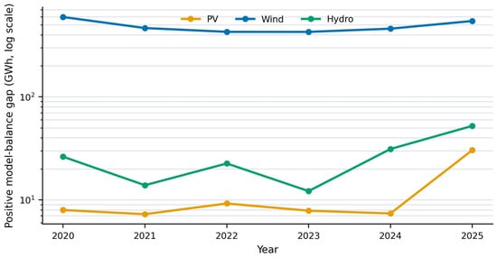
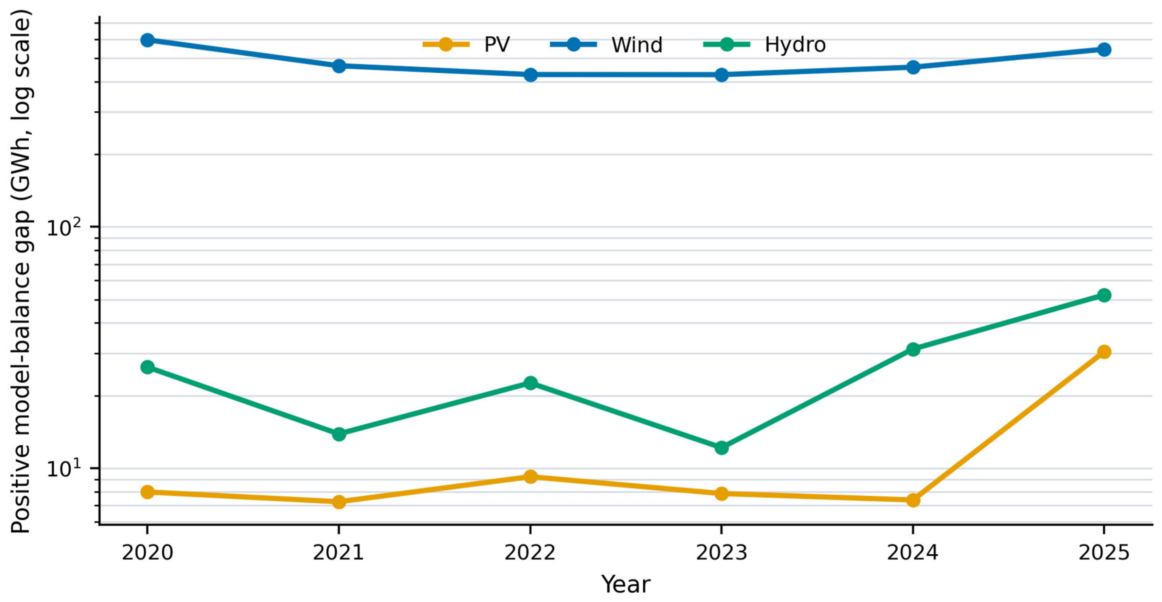
The capacity represented in the annual records changed materially during the study. Combined nameplate capacity increased from 444.294 MW in 2020 to 587.241 MW in 2025. PV capacity rose from 12.752 to 56.475 MW, WE from 409.008 to 497.952 MW, and HE from 22.534 to 32.814 MW, with non-monotonic changes in the annual source roster. Table 4 therefore reports both absolute and capacity-normalized results. Figure 1 shows the annual positive gap by technology.

Table 4. Annual data coverage and positive model-balance gap across all technologies.

Year	Complete Records	Represented Capacity [MW]	Metered [GWh]	Modelled [GWh]	Positive Gap [GWh]	Gap Rate [%]	Intensity [MWh/ (MW·Year)]
2020	243	444.294	319.116	947.996	629.860	66.44	1417.7
2021	245	486.879	532.031	1017.275	486.542	47.83	999.3
2022	239	524.263	639.038	1097.738	459.560	41.86	876.6
2023	250	508.873	613.004	1058.410	447.351	42.27	879.1
2024	258	513.938	586.414	1082.796	497.483	45.94	968.0
2025	278	587.241	583.822	1210.461	627.508	51.84	1068.6

Figure 1. Annual positive model-balance gap by technology. A logarithmic axis is used because WE values are substantially larger than PV and HE values.

The annual model values total 6414.677 GWh, while recorded grid injection totals 3273.425 GWh. Their signed net difference is 3141.252 GWh. Applying the positive operator separately to the 1513 source-year comparisons yields 3148.304 GWh. Negative differences occur in 193 records and have a combined magnitude of 7.051 GWh. These totals satisfy the signed/positive/negative accounting identity before rounding; displayed totals are rounded independently. WE contributes 2919.944 GWh (92.75%) of the positive gap, HE 158.276 GWh (5.03%), and PV 70.083 GWh (2.23%). The 3148.304 GWh result is therefore the sum of positive model–injection differences across the supplied source-year records.

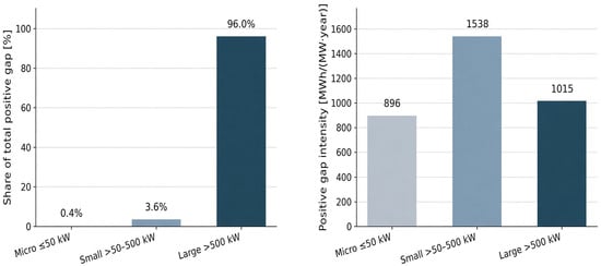
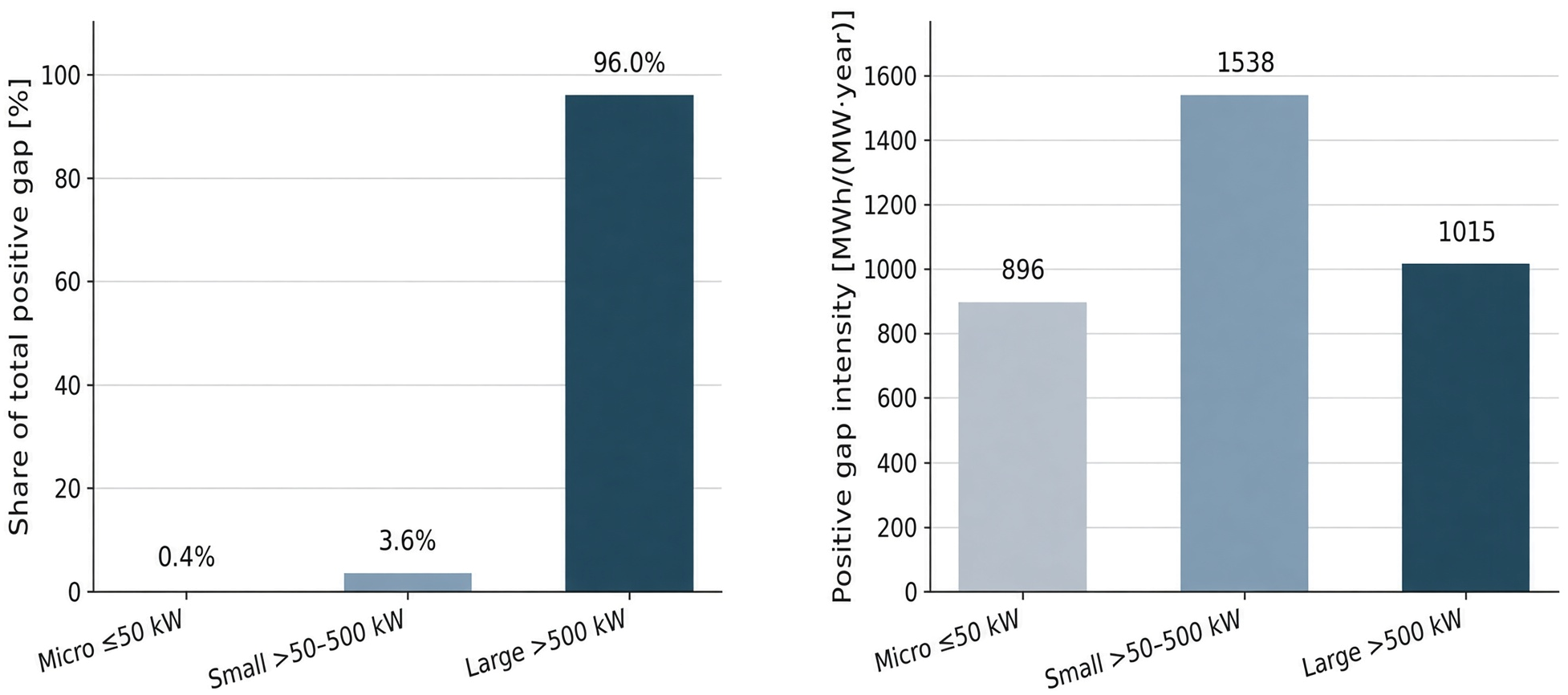
The negative component is small at total-system level but material for micro sources. For that class, the positive gap is 13.322 GWh, the negative-difference magnitude is 6.923 GWh, and the signed balance is 6.399 GWh. Positive-part accounting therefore cannot replace the signed balance when model agreement or class-level differences are discussed. It is retained specifically for the positive-resource definition used by the EV scenario model. Table 5 reports the six-year results by source capacity class. Figure 2 shows each capacity class’s share of the total positive gap and its capacity-normalized positive-gap intensity.

Table 5. Six-year results by source capacity class.

Capacity Class	n	Capacity Exposure [MW·Year]	Metered [GWh]	Modelled [GWh]	Positive Gap [GWh]	Gap Rate [%]	Intensity [MWh/ (MW·Year)]	Share [%]
Micro ≤50 kW	857	14.875	26.281	32.680	13.322	40.76	895.6	0.42
Small >50–500 kW	358	73.156	42.703	155.105	112.531	72.55	1538.2	3.57
Large >500 kW	298	2977.457	3204.441	6226.892	3022.451	48.54	1015.1	96.00

Figure 2. Contribution of each capacity class to the total positive model-balance gap and the capacity-normalized gap intensity.

Large sources contributed 96.00% of the absolute positive gap. Normalization changed the comparison: small sources had the highest gap rate (72.55%) and intensity (1538.2 MWh/(MW·year)), whereas large sources had a lower rate (48.54%) and intensity (1015.1 MWh/(MW·year)). Capacity class therefore affects absolute system relevance and per-capacity performance differently. Table 6 provides a quantitative breakdown of the positive differences between potential electricity generation and actual electricity injected into the grid, disaggregated by generation technology and installed capacity class.

Table 6. Six-year positive model-balance gap by technology and capacity class.

Technology	Capacity Class	n	Capacity Exposure [MW·Year]	Positive Gap [GWh]	Gap Rate [%]	Intensity [MWh/ (MW·Year)]
PV	Micro ≤50 kW	461	4.966	2.144	46.52	431.8
PV	Small >50–500 kW	137	25.960	18.114	74.50	697.8
PV	Large >500 kW	62	101.683	49.825	53.51	490.0
WE	Micro ≤50 kW	81	0.730	1.383	90.16	1895.5
WE	Small >50–500 kW	62	19.885	36.467	87.23	1833.9
WE	Large >500 kW	204	2811.064	2882.094	48.77	1025.3
HE	Micro ≤50 kW	315	9.179	9.794	36.91	1067.0
HE	Small >50–500 kW	159	27.311	57.949	65.12	2121.8
HE	Large >500 kW	32	64.710	90.533	40.45	1399.1

3.2. Capacity-Normalized Potential–Injection Differences

Capacity-normalized diagnostics compare modelled potential and recorded grid injection per unit of installed capacity. Table 7 reports these difference metrics by technology.

Table 7. Descriptive difference metrics for capacity-normalized annual potential and grid-injection yields.

Technology	n	MBE [MWh/ (MW·Year)]	MAE [MWh/ (MW·Year)]	RMSE [MWh/ (MW·Year)]	nMAE [%]	nRMSE [%]	Metered > Modelled [% Records]
PV	660	404.4	466.9	573.8	87.4	107.5	8.8
WE	347	1454.8	1469.4	1558.0	226.9	240.6	1.4
HE	506	638.3	2027.1	3545.5	85.5	149.6	25.7

The root mean square error for hydropower in Table 7 is large relative to the mean capacity-normalized metered yield because the HE comparison mixes assumed capacity-factor reference levels with metered injection across a heterogeneous set of small and large plants, and because a substantial share of HE records have injection above the model (negative differences). RMSE penalizes large individual deviations in either direction. It is a descriptive difference metric between potential and injection, not a measure of forecast error against unconstrained production. The nine records with injection above nameplate × hours contribute to the negative tail and therefore to RMSE; their retention increases the diagnostic magnitude without increasing the positive gap.

The mean capacity-normalized potential–injection difference is positive for all three technologies. This describes the two compared series; it cannot establish that the entire difference is model error, because generation potential and recorded grid injection are different physical quantities. The normalized differences are largest for WE. Grid injection exceeds the reference model in 58 PV records (8.8%), five WE records (1.4%), and 130 HE records (25.7%). Keeping these records in the signed diagnostics prevents positive-part accounting from being mistaken for independent model validation.

HE RMSE is 149.6% of its mean recorded yield of 2370.3 MWh/(MW·year). The nine high-injection records account for 66.25% of the sum of squared yield differences, so squaring strongly amplifies their influence. After exclusion, RMSE is 2078.4 MWh/(MW·year), or 98.8% of the remaining mean recorded yield. The reduction identifies a data-quality contribution, but substantial disagreement remains and cannot be attributed to curtailment without hydraulic, operating and meter-boundary evidence.

3.3. EV Charging Scenarios for 2025

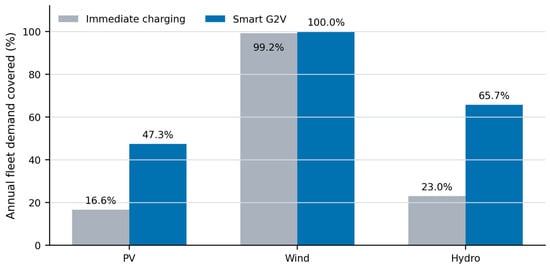
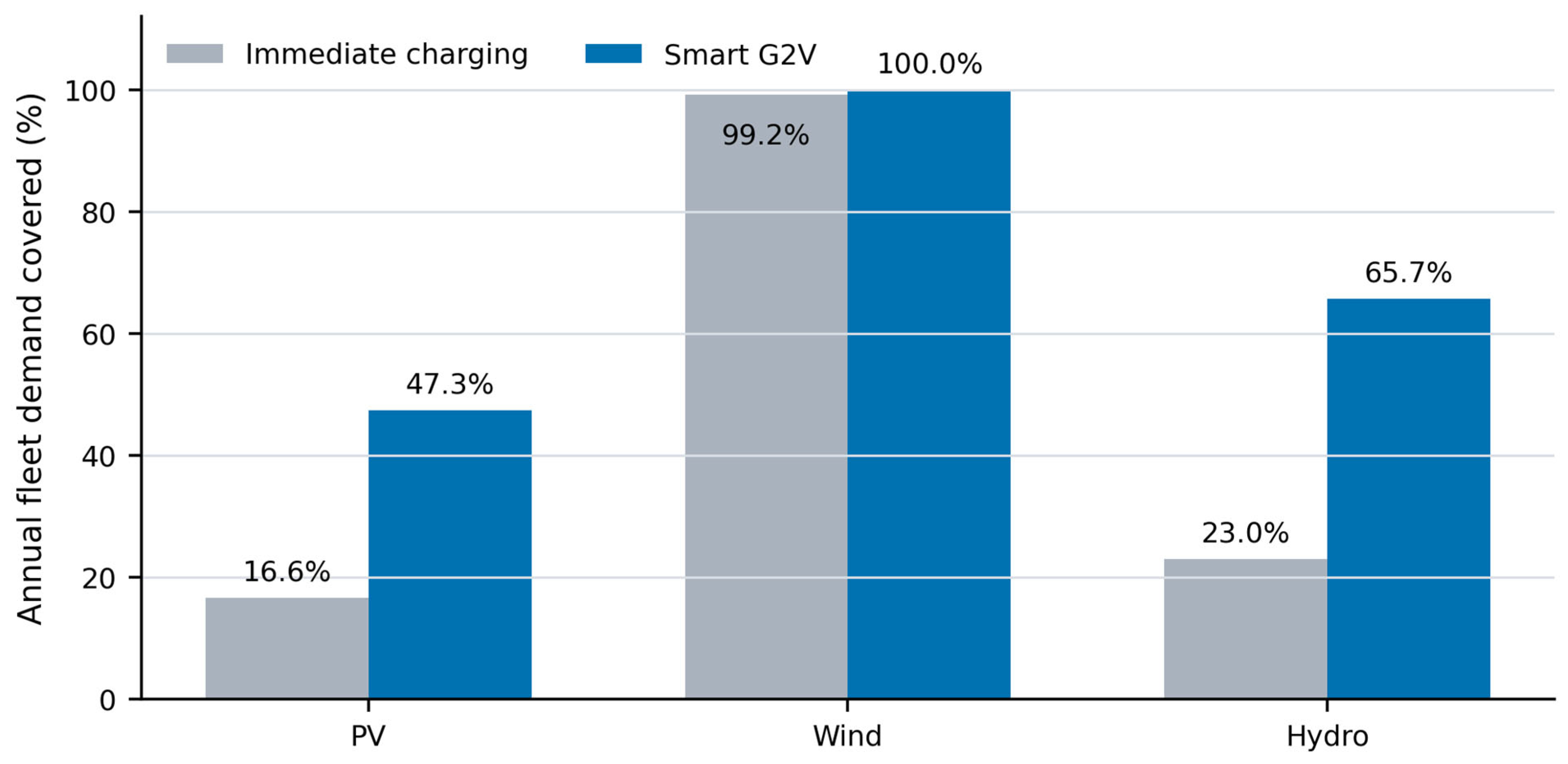
The fixed reference fleet demanded 53.308 GWh/year in each scenario. Table 8 reports all nine 2025 technology–capacity combinations. In micro and small scenarios, available energy limited charging. In the large-source WE scenario, power and window constraints capped technically absorbable energy at 249.660 GWh even though the positive gap was 539.734 GWh. Figure 3 compares immediate charging and Smart G2V coverage in the 2025 large-source scenarios.

Table 8. Annual EV results for 2025 at f = 1. V2G is hypothetical grid-side discharge under the supplied compatibility flags and cycling budget, not verified delivery or net demand.

Technology	Source Class	Positive Gap [GWh]	Immediate [GWh]	Smart G2V [GWh]	V2G [GWh]	Demand Covered by Smart G2V [%]
PV	Micro	0.174	0.055	0.157	0.000	0.29
PV	Small	2.073	0.653	1.866	0.000	3.50
PV	Large	28.153	8.833	25.238	0.000	47.34
WE	Micro	0.606	0.191	0.546	0.000	1.02
WE	Small	4.514	1.422	4.062	0.000	7.62
WE	Large	539.734	52.883	53.308	9.274	100.00
HE	Micro	1.744	0.550	1.570	0.000	2.95
HE	Small	11.612	3.658	10.451	0.000	19.61
HE	Large	38.897	12.252	35.007	0.000	65.67

Figure 3. Annual reference-fleet demand covered by immediate charging and Smart G2V in the 2025 large-source scenarios.

Large-source Smart G2V coverage is 47.34% for PV, 100.00% for WE and 65.67% for HE at f = 1. The V2G discharge ceiling is 9.274 GWh for large WE and zero for the other 2025 cases. Correcting charging/discharging boundaries does not change that baseline ceiling because its battery-cycle limit binds, but it requires 11.450 GWh of replenishment input. Including traction charging gives 64.758 GWh, or 25.94% of accessible energy and 12.00% of the original positive WE gap. These accounting ratios do not establish hourly deliverability or profitability. Under annual cycling budgets of 10 and 25 equivalent full cycles, the V2G ceilings fall to 1.694 and 4.235 GWh.

3.4. Sensitivity Results

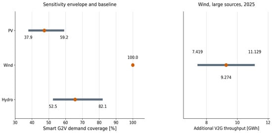
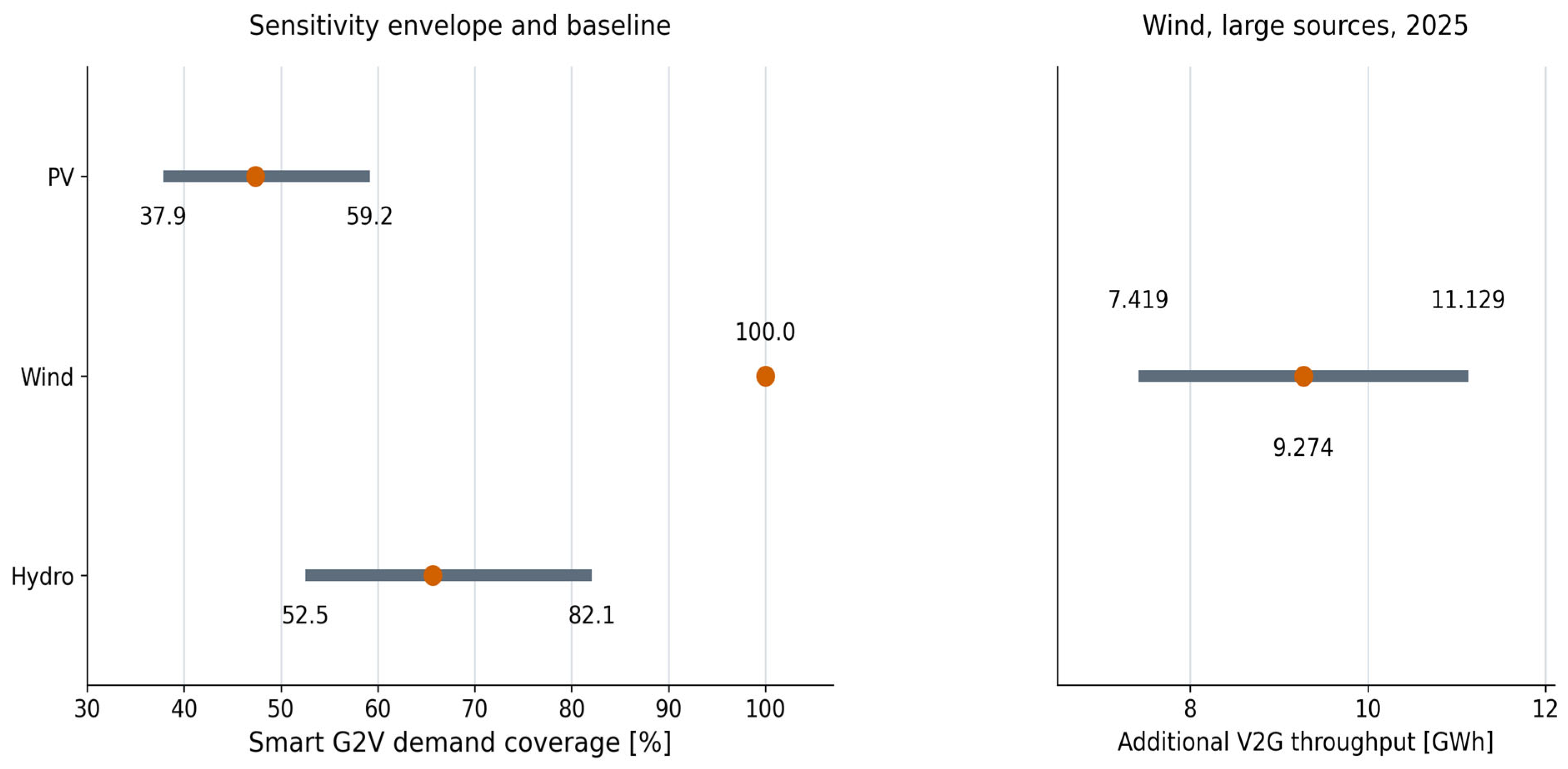
The sensitivity results show how the positive gap and the EV coverage respond to the stated parameter changes. Table 9 gives the baseline values and the deterministic envelopes. Figure 4 shows the one-at-a-time sensitivity envelopes for Smart G2V coverage and additional V2G throughput.

Table 9. Baseline results and deterministic sensitivity envelopes.

Metric	Baseline	Sensitivity Envelope	Perturbation Basis
Six-year positive model-balance gap	3148.304 GWh	1874.982–4429.287 GWh	All Emodel values scaled by −20%/+20%
PV large, 2025 Smart G2V coverage	47.34%	37.87–59.18%	One parameter at a time, ±20%
WE large, 2025 Smart G2V coverage	100.00%	100% throughout	One parameter at a time, ±20%
HE large, 2025 Smart G2V coverage	65.67%	52.54–82.09%	One parameter at a time, ±20%
WE large, 2025 V2G throughput	9.274 GWh	7.419–11.129 GWh	One parameter at a time, ±20%
WE large, source-side use of accessible energy including V2G replenishment	25.94%	21.62–32.42%	One parameter at a time, ±20%
Common a = 0.60, 2025 large-source Smart G2V coverage	PV 47.53%; WE 100.00%; HE 65.67%	PV + 0.19 percentage points; WE and HE unchanged	Common availability; technology windows retained

Figure 4. One-at-a-time sensitivity envelopes for Smart G2V demand coverage and hypothetical grid-side V2G discharge in the 2025 large-source scenarios. Orange points show baseline values. Compatibility and cycling-cost assumptions remain scenario conditions.

The original one-at-a-time coverage envelopes are reproduced: 37.87–59.18% for PV, 100% throughout for WE and 52.54–82.09% for HE. The V2G discharge envelope is 7.419–11.129 GWh under the hypothetical four-model compatibility case. The corrected source-side utilization ratio in Table 9 is [Σx_G2V + Σz_V2G/(η_chη_dis)]/ΣE_acc, so charging and discharge energies are not added across different boundaries. Its envelope is 21.62–32.42%. Supplement S6 lists parameter-specific results. Combined scenarios are recalculated explicitly rather than assumed to lie within one-at-a-time envelopes. For example, f = 0.25, WE CF = 0.192, a = 0.60 and h = 6 h/day give PV/WE/HE coverage of 11.88%/99.80%/16.42% and WE V2G discharge of 5.853 GWh.

Scaling all annual generation-potential values by ±20% changes the cumulative positive gap to 1874.982–4429.287 GWh. This quantifies dependence on the reference production level, including the aggregate influence of resource and performance assumptions; it does not isolate the uncertainty of any particular regional profile. In the EV screen, PV and HE demand coverage respond to annual demand, charging efficiency, capture coefficient, and the positive-gap input. WE remains at 100% demand coverage across the reported one-at-a-time screen because the resource exceeds fleet demand, while V2G participation, discharge efficiency, and the cycle limit govern its additional throughput.

4. Discussion

4.1. Interpretation and Contribution

The regional DSO balance identifies two different priorities. Large sources dominate the absolute positive potential–injection gap, whereas small sources have the highest gap rate and intensity per unit of installed capacity. Presenting both measures therefore separates scale from relative utilization of the modelled generation potential. This is the main empirical finding of the renewable-energy analysis. Formal regional assignment connects each source to its model profile, but the annual wind and hydro levels still depend on CF. The result should be interpreted within this explicitly documented model structure.

The alternative explanations of constrained energy and mismatch between model and operation cannot be separated solely from a potential–injection difference. Nor do large MBE, MAE, or RMSE values demonstrate that the full 3148.304 GWh is a modelling error: they compare potential with injection, not two observations of unconstrained production. The calculation establishes the positive gap conditional on its reference assumptions. Its causal decomposition would require dispatch/set-point logs, equipment availability and outage records, own-consumption and loss information, and comparable meter boundaries. Operationally recoverable energy is consequently a subset to be identified, rather than a quantity independently measured here.

The EV analysis gives the regional energy balance a defined use scenario. The same reference fleet is tested against each technology–year–capacity combination, and charging is limited by demand, charger power, availability, connection capacity, losses, and battery constraints. This approach makes the reported demand-coverage fractions traceable to the stated annual assumptions. In relation to Szinai et al. [43], Dixon et al. [44], and Saadatmandi et al. [45], the comparison concerns analytical purpose: operating cost, carbon emissions, or technology-specific curtailment versus utilization of a multi-technology DSO reference balance. The endpoints are different, so the percentages are not treated as cross-study measures of charging performance.

4.2. Temporal, Network, and Data Limitations

The EV results are annual screening values. Annual energy and assumed daily windows cannot demonstrate hourly or 15 min coincidence between renewable production and plugged-in vehicles. They also do not resolve feeder constraints, transformer loading, voltage, congestion, or the distance between sources and chargers. Immediate charging uses an assumed overlap coefficient rather than measured mobility. Smart G2V and V2G values should therefore be read as model-conditioned bounds, not dispatch schedules.

The supplied annual records cannot establish daily alignment between generation and plugged-in vehicles. Figure 1 therefore remains an annual comparison; no monthly generation or charging-output series is added. Applying a shared regional profile to both annual series would create a reconstruction rather than independent temporal evidence. Regional PV irradiation sums affect annual reference yields, whereas normalized WE/HE profiles only allocate fixed annual totals and do not affect annual gaps or EV coverage. Even a monthly plot would not resolve hourly coincidence. Reduced overlap can lower immediate charging, and unmet daily charging windows can lower Smart G2V coverage. The eligibility tests quantify one dimension of that limitation without pretending to reconstruct chronology.

Changes in represented capacity are included at the annual level, but exact commissioning dates are absent. Capacity-normalized indicators reduce scale effects without reconstructing part-year availability. The lack of consistently linked source identifiers also prevents a balanced longitudinal panel. The retained formal DSO regional keys support profile assignment; they do not establish national representativeness or meteorological uniformity within every operating area. PV and wind profiles in the supplied documentation are reference profiles rather than independently measured weather series for every year. Some 2025 hydro profiles are regional estimates. These distinctions limit claims about year-specific local production.

The deterministic sensitivity envelopes are not statistical uncertainty intervals. They show the scale of parameter dependence under symmetric perturbations. A probabilistic uncertainty analysis would require empirical distributions or justified priors for renewable-model error, charging availability, annual distance, consumption, connection capacity, user participation, and battery operation.

This is a single-operator, changing-roster case study without independent resource validation. Its numerical totals, technology shares and priority classes are not demonstrated to transfer to other networks. The transferable element is the accounting procedure: paired annual differences, positive and signed totals, normalization, explicit eligibility assumptions and constrained allocation. Applying that procedure elsewhere requires comparable records and separately justified reference models.

4.3. Implications for Further Analysis

The screening results can prioritize follow-up data collection. Large WE records deserve attention because they dominate the absolute gap; small WE and HE records deserve attention because their per-capacity intensities are high. The next analytical stage should combine time-stamped available-power estimates, metered output, dispatch and outage labels, feeder topology, transformer limits, charger locations, vehicle arrival and departure times, and dynamic SOC. An hourly or 15 min optimization could then estimate avoided curtailment, network feasibility, charging cost, and battery degradation instead of annual energy throughput alone.

For an operator or charging planner, the first action is to reconcile the nine flagged HE capacity/energy records and the ten non-standard PV model values. Large WE records are then priorities for site-specific resource, commissioning and constraint-event checks because their residual dominates this dataset. Small sources warrant capacity-normalized checks. Any charging pilot should measure coincident generation, plugged-in availability, feeder headroom and SOC at hourly or 15 min resolution before capacity is sized. A V2G pilot additionally needs vehicle/charger/protocol approval, a replenishment energy balance, an ageing budget and a tariff assessment. Annual residuals alone do not justify an investment size or an estimate of avoided curtailment. The annual screen does not indicate whether residual energy is available during vehicle connection windows; hourly or 15 min data are required to assess temporal coincidence.

5. Conclusions

For 1513 complete source-year records in 2020–2025, the positive reference-model–injection difference is 3148.304 GWh. Large sources contribute 96.00% and WE contributes 92.75% at CF = 0.24; small sources have the highest normalized gap rate and intensity. These results are conditional annual benchmarks. For the 20,043-vehicle reference fleet, large-source 2025 Smart G2V coverage is 47.34%, 100.00% and 65.67% for PV, WE and HE when f = 1. At f = 0.10, it is 4.75%, 91.12% and 6.57%. Thus, the choice of eligible share materially changes the charging interpretation. The hypothetical four-model V2G ceiling of 9.274 GWh is subject to configuration, cycling and economic constraints and is not demonstrated grid delivery. These coverage values remain conditional on the stated eligibility fraction, capture coefficient, and annual aggregation; they do not constitute an estimate of realized charging potential. This qualification applies throughout: results are conditional accounting benchmarks, not estimates of recoverable energy or realized charging potential.

Reference assumptions materially affect the results. Scaling all modelled generation by ±20% yields 1874.982–4429.287 GWh; wind-only sensitivity and the alternative PV-label calculation separate two sources of dependence. Table 7 retains all 506 HE records. A separate sensitivity analysis excluding nine implausible HE records reduces RMSE from 3545.5 to 2078.4 MWh/(MW·year) and changes the signed balance but leaves the positive-gap total unchanged because each excluded record has a negative model–injection difference. These checks improve traceability without validating the reference models. Localized wind-resource reconstruction and independently justified capacity factors remain necessary for site-level production estimates.

The practical outcome is a prioritized measurement and data-reconciliation programme. Operators should establish comparable meter boundaries and operation periods before attributing residuals to constraints. Charging planners should test coincidence and network feasibility before sizing infrastructure, and include losses, vehicle-specific compatibility and battery wear in V2G assessment. The annual screen supports those next steps; it does not quantify measured curtailment, verified recoverable energy or realized economic savings.

References

- Bird, L.; Lew, D.; Milligan, M.; Carlini, E.M.; Estanqueiro, A.; Flynn, D.; Gomez-Lazaro, E.; Holttinen, H.; Menemenlis, N.; Orths, A.; et al. Wind and solar energy curtailment: A review of international experience. Renew. Sustain. Energy Rev. 2016, 65, 577–586. [Google Scholar] [CrossRef] [Scilit]
- Li, C.; Shi, H.; Cao, Y.; Wang, J.; Kuang, Y.; Tan, Y.; Wei, J. Comprehensive review of renewable energy curtailment and avoidance: A specific example in China. Renew. Sustain. Energy Rev. 2015, 41, 1067–1079. [Google Scholar] [CrossRef] [Scilit]
- O’Shaughnessy, E.; Cruce, J.; Xu, K. Too much of a good thing? Global trends in the curtailment of solar PV. Sol. Energy 2020, 208, 1068–1077. [Google Scholar] [CrossRef] [Scilit] [PubMed]
- Lund, H.; Mathiesen, B.V. Energy system analysis of 100% renewable energy systems—The case of Denmark in years 2030 and 2050. Energy 2009, 34, 524–531. [Google Scholar] [CrossRef] [Scilit]
- Denholm, P.; Hand, M. Grid flexibility and storage required to achieve very high penetration of variable renewable electricity. Energy Policy 2011, 39, 1817–1830. [Google Scholar] [CrossRef] [Scilit]
- Victoria, M.; Zhu, K.; Brown, T.; Andresen, G.B.; Greiner, M. The role of storage technologies throughout the decarbonisation of the sector-coupled European energy system. Energy Convers. Manag. 2019, 201, 111977. [Google Scholar] [CrossRef] [Scilit]
- Brown, T.; Schlachtberger, D.; Kies, A.; Schramm, S.; Greiner, M. Synergies of sector coupling and transmission reinforcement in a cost-optimised, highly renewable European energy system. Energy 2018, 160, 720–739. [Google Scholar] [CrossRef] [Scilit]
- Zappa, W.; Junginger, M.; van den Broek, M. Is a 100% renewable European power system feasible by 2050? Appl. Energy 2019, 233–234, 1027–1050. [Google Scholar] [CrossRef] [Scilit]
- Rasmussen, M.G.; Andresen, G.B.; Greiner, M. Storage and balancing synergies in a fully or highly renewable pan-European power system. Energy Policy 2012, 51, 642–651. [Google Scholar] [CrossRef] [Scilit]
- Heide, D.; Greiner, M.; von Bremen, L.; Hoffmann, C. Reduced storage and balancing needs in a fully renewable European power system with excess wind and solar power generation. Renew. Energy 2011, 36, 2515–2523. [Google Scholar] [CrossRef] [Scilit]
- Papaefthymiou, G.; Dragoon, K. Towards 100% renewable energy systems: Uncapping power system flexibility. Energy Policy 2016, 92, 69–82. [Google Scholar] [CrossRef] [Scilit]
- Lund, P.D.; Lindgren, J.; Mikkola, J.; Salpakari, J. Review of energy system flexibility measures to enable high levels of variable renewable electricity. Renew. Sustain. Energy Rev. 2015, 45, 785–807. [Google Scholar] [CrossRef] [Scilit]
- Peker, M.; Kocaman, A.S.; Kara, B.Y. Benefits of transmission switching and energy storage in power systems with high renewable energy penetration. Appl. Energy 2018, 228, 1182–1197. [Google Scholar] [CrossRef] [Scilit]
- Laimon, M. Renewable energy curtailment: A problem or an opportunity? Results Eng. 2025, 26, 104925. [Google Scholar] [CrossRef] [Scilit]
- Soto-Valle, R.; Usuba, J. Wind Energy Curtailment: Historical Case Study. Energies 2026, 19, 334. [Google Scholar] [CrossRef] [Scilit]
- Huld, T.; Amillo, A.M.G. Estimating PV module performance over large geographical regions: The role of irradiance, air temperature, wind speed and solar spectrum. Energies 2015, 8, 5159–5181. [Google Scholar] [CrossRef] [Scilit]
- De Soto, W.; Klein, S.A.; Beckman, W.A. Improvement and validation of a model for photovoltaic array performance. Sol. Energy 2006, 80, 78–88. [Google Scholar] [CrossRef] [Scilit]
- Fahim, S.R.; Hasanien, H.M.; Turky, R.A.; Abdel Aleem, S.H.E.; Ćalasan, M. A comprehensive review of photovoltaic modules models and algorithms used in parameter extraction. Energies 2022, 15, 8941. [Google Scholar] [CrossRef] [Scilit]
- Rajesh, R.; Mabel, M.C. A comprehensive review of photovoltaic systems. Renew. Sustain. Energy Rev. 2015, 51, 231–248. [Google Scholar] [CrossRef] [Scilit]
- Jordan, D.C.; Kurtz, S.R. Photovoltaic degradation rates—An analytical review. Prog. Photovolt. Res. Appl. 2013, 21, 12–29. [Google Scholar] [CrossRef] [Scilit]
- Skoplaki, E.; Palyvos, J.A. Operating temperature of photovoltaic modules: A survey of pertinent correlations. Renew. Energy 2009, 34, 23–29. [Google Scholar] [CrossRef] [Scilit]
- Skoplaki, E.; Boudouvis, A.G.; Palyvos, J.A. A simple correlation for the operating temperature of photovoltaic modules of arbitrary mounting. Sol. Energy Mater. Sol. Cells 2008, 92, 1393–1402. [Google Scholar] [CrossRef] [Scilit]
- Carta, J.A.; Ramírez, P.; Velázquez, S. A review of wind speed probability distributions used in wind energy analysis: Case studies in the Canary Islands. Renew. Sustain. Energy Rev. 2009, 13, 933–955. [Google Scholar] [CrossRef] [Scilit]
- Murthy, K.S.R.; Rahi, O.P. A comprehensive review of wind resource assessment. Renew. Sustain. Energy Rev. 2017, 72, 1320–1342. [Google Scholar] [CrossRef] [Scilit]
- Lydia, M.; Suresh Kumar, S.; Selvakumar, A.I.; Prem Kumar, G.E. A comprehensive review on wind turbine power curve modeling techniques. Renew. Sustain. Energy Rev. 2014, 30, 452–460. [Google Scholar] [CrossRef] [Scilit]
- Bilendo, F.; Meyer, A.; Badihi, H.; Lu, N.; Cambron, P.; Jiang, B. Applications and Modeling Techniques of Wind Turbine Power Curve for Wind Farms—A Review. Energies 2023, 16, 180. [Google Scholar] [CrossRef] [Scilit]
- Saint-Drenan, Y.M.; Besseau, R.; Jansen, M.; Staffell, I.; Troccoli, A.; Dubus, L.; Schmidt, J.; Gruber, K.; Simões, S.G.; Heier, S. A parametric model for wind turbine power curves incorporating environmental conditions. Renew. Energy 2020, 157, 754–768. [Google Scholar] [CrossRef] [Scilit]
- Igliński, B.; Iglińska, A.; Koziński, G.; Skrzatek, M.; Buczkowski, R. Wind energy in Poland—History, current state, surveys, Renewable Energy Sources Act, SWOT analysis. Renew. Sustain. Energy Rev. 2016, 64, 19–33. [Google Scholar] [CrossRef] [Scilit]
- Pryor, S.C.; Barthelmie, R.J. Climate change impacts on wind energy: A review. Renew. Sustain. Energy Rev. 2010, 14, 430–437. [Google Scholar] [CrossRef] [Scilit]
- Hamududu, B.; Killingtveit, A. Assessing climate change impacts on global hydropower. Energies 2012, 5, 305–322. [Google Scholar] [CrossRef] [Scilit]
- Wasti, A.; Ray, P.; Wi, S.; Folch, C.; Ubierna, M.; Karki, P. Climate change and the hydropower sector: A global review. WIREs Clim. Change 2022, 13, e757. [Google Scholar] [CrossRef] [Scilit]
- Turner, S.W.D.; Hejazi, M.; Kim, S.H.; Clarke, L.; Edmonds, J. Climate impacts on hydropower and consequences for global electricity supply investment needs. Energy 2017, 141, 2081–2090. [Google Scholar] [CrossRef] [Scilit]
- Klein, S.J.W.; Fox, E.L.B. A review of small hydropower performance and cost. Renew. Sustain. Energy Rev. 2022, 169, 112898. [Google Scholar] [CrossRef] [Scilit]
- Kasperek, R. Perspektywy rozwoju energetyki wodnej w Polsce [Prospects for the Development of Hydropower in Poland]. Pol. J. Sustain. Dev. 2020, 24, 29–38. [Google Scholar] [CrossRef] [Scilit]
- Yüksel, I. Hydropower for sustainable water and energy development. Renew. Sustain. Energy Rev. 2010, 14, 462–469. [Google Scholar] [CrossRef] [Scilit]
- Zarfl, C.; Lumsdon, A.E.; Berlekamp, J.; Tydecks, L.; Tockner, K. A global boom in hydropower dam construction. Aquat. Sci. 2015, 77, 161–170. [Google Scholar] [CrossRef] [Scilit]
- Tahseen, S.; Karney, B.W. Reviewing and critiquing published approaches to the sustainability assessment of hydropower. Renew. Sustain. Energy Rev. 2017, 67, 225–234. [Google Scholar] [CrossRef] [Scilit]
- Sobik, B. Wykorzystanie fotowoltaiki jako źródła pokrywającego zapotrzebowanie szczytowe w okresie letnim w Krajowym Systemie Elektroenergetycznym [Use of Photovoltaics as a Source Covering Peak Demand in Summer in the National Power System]. Zesz. Nauk. Inst. Gospod. Surowcami Miner. Energ. Pol. Akad. Nauk 2019, 109, 123–136. [Google Scholar] [CrossRef]
- Richardson, D.B. Electric vehicles and the electric grid: A review of modeling approaches, impacts, and renewable energy integration. Renew. Sustain. Energy Rev. 2013, 19, 247–254. [Google Scholar] [CrossRef] [Scilit]
- Mwasilu, F.; Justo, J.J.; Kim, E.K.; Do, T.D.; Jung, J.W. Electric vehicles and smart grid interaction: A review on vehicle to grid and renewable energy sources integration. Renew. Sustain. Energy Rev. 2014, 34, 501–516. [Google Scholar] [CrossRef] [Scilit]
- Sadeghian, O.; Oshnoei, A.; Mohammadi-Ivatloo, B.; Vahidinasab, V.; Anvari-Moghaddam, A. A comprehensive review on electric vehicles smart charging: Solutions, strategies, technologies, and challenges. J. Energy Storage 2022, 54, 105241. [Google Scholar] [CrossRef] [Scilit]
- Barman, P.; Dutta, L.; Bordoloi, S.; Kalita, A.; Buragohain, P.; Bharali, S.; Azzopardi, B. Renewable energy integration with electric vehicle technology: A review of the existing smart charging approaches. Renew. Sustain. Energy Rev. 2023, 183, 113518. [Google Scholar] [CrossRef] [Scilit]
- Szinai, J.K.; Sheppard, C.J.R.; Abhyankar, N.; Gopal, A.R. Reduced grid operating costs and renewable energy curtailment with electric vehicle charge management. Energy Policy 2020, 136, 111051. [Google Scholar] [CrossRef] [Scilit]
- Dixon, J.; Bukhsh, W.; Edmunds, C.; Bell, K. Scheduling electric vehicle charging to minimise carbon emissions and wind curtailment. Renew. Energy 2020, 161, 1072–1091. [Google Scholar] [CrossRef] [Scilit]
- Saadatmandi, S.; Chicco, G.; Favenza, A.; Mozzato, A.; Giordano, F.; Arnone, M. Smart electric vehicle charging for reducing photovoltaic energy curtailment. Electr. Power Syst. Res. 2024, 230, 110181. [Google Scholar] [CrossRef] [Scilit]
- Lund, H.; Kempton, W. Integration of renewable energy into the transport and electricity sectors through V2G. Energy Policy 2008, 36, 3578–3587. [Google Scholar] [CrossRef] [Scilit]
- Kempton, W.; Tomić, J. Vehicle-to-grid power fundamentals: Calculating capacity and net revenue. J. Power Sources 2005, 144, 268–279. [Google Scholar] [CrossRef] [Scilit]
- Tan, K.M.; Ramachandaramurthy, V.K.; Yong, J.Y. Integration of electric vehicles in smart grid: A review on vehicle to grid technologies and optimization techniques. Renew. Sustain. Energy Rev. 2016, 53, 720–732. [Google Scholar] [CrossRef] [Scilit]
- Sovacool, B.K.; Axsen, J.; Kempton, W. The future promise of vehicle-to-grid (V2G) integration: A sociotechnical review and research agenda. Annu. Rev. Environ. Resour. 2017, 42, 377–406. [Google Scholar] [CrossRef] [Scilit]
- Das, H.S.; Rahman, M.M.; Li, S.; Tan, C.W. Electric vehicles standards, charging infrastructure, and impact on grid integration: A technological review. Renew. Sustain. Energy Rev. 2020, 120, 109618. [Google Scholar] [CrossRef] [Scilit]
- İnci, M.; Çelik, Ö.; Lashab, A.; Bayındır, K.Ç.; Vasquez, J.C.; Guerrero, J.M. Power System Integration of Electric Vehicles: A Review on Impacts and Contributions to the Smart Grid. Appl. Sci. 2024, 14, 2246. [Google Scholar] [CrossRef] [Scilit]
- Flasza, J.; Matuszczyk, P. Elektromobilność w Polsce a systemy OZE [Electromobility in Poland and Renewable Energy Systems]. Prz. Elektrotech. 2018, 94, 33–36. [Google Scholar] [CrossRef] [Scilit]
- Blumberg, G.; Broll, R.; Weber, C. The impact of electric vehicles on the future European electricity system—A scenario analysis. Energy Policy 2022, 161, 112751. [Google Scholar] [CrossRef] [Scilit]
- IRENA. Innovation Outlook: Smart Charging for Electric Vehicles; International Renewable Energy Agency: Abu Dhabi, United Arab Emirates, 2019; Available online: https://www.irena.org/publications/2019/May/Innovation-Outlook-Smart-Charging (accessed on 17 August 2026).
- US Department of Energy. Vehicles-to-Grid Integration Assessment Report; DOE: Washington, DC, USA, 2025. Available online: https://www.energy.gov/cmei/vehicles/articles/vehicle-grid-integration-assessment-report (accessed on 17 August 2026).
- EV Database. Energy Consumption of Electric Vehicles. Available online: https://ev-database.org/cheatsheet/energy-consumption-electric-car (accessed on 17 August 2026).
- Otwarte Dane. API dla bazy Centralnej Ewidencji Pojazdów i Kierowców (CEPiK). Available online: https://dane.gov.pl/pl/dataset/1558 (accessed on 17 August 2026).
- Niu, S.; Liu, W.; Liu, C.; Jia, C.; Liserre, M.; Chau, K.T. A non-intrusive integration of wireless chargers into electric vehicles: 95.60% dc-dc efficiency at 0.51 LD-to-CL ratio with on-vehicle demonstration. eTransportation 2026, 27, 100547. [Google Scholar] [CrossRef] [Scilit]
- Nissan. Nissan Approves Enhanced Fermata Energy FE-20 Bidirectional Charger V2XPlatform for Use with Nissan LEAF. 28 August 2024. Available online: https://usa.nissannews.com/en-US/releases/nissan-approves-enhanced-fermata-energy-fe-20-bidirectional-charger-and-v2x-platform-for-use-with-nissan-leaf (accessed on 27 October 2026).
- Kia. Kia’s EV6 Reimagines the Electric Vehicle Ownership Experience. 2021. Available online: https://prod2-press.kia.com/eu/en/home/media-resouces/press-releases/2021/Kias-EV6-reimagines-the-electric-vehicle-ownership-experience.html (accessed on 27 October 2026).
- Tesla. Tesla Powershare. Available online: https://www.tesla.com/support/powershare (accessed on 27 October 2026).
Disclaimer/Publisher’s Note: The statements, opinions and data contained in all publications are solely those of the individual author(s) and contributor(s) and not of MDPI and/or the editor(s). MDPI and/or the editor(s) disclaim responsibility for any injury to people or property resulting from any ideas, methods, instructions or products referred to in the content. |
© 2026 by the authors. Licensee MDPI, Basel, Switzerland. This article is an open access article distributed under the terms and conditions of the Creative Commons Attribution (CC BY) license.