


Abstract
Electro-hydraulic volumetric control is increasingly used in industry due to its decreasing implementation costs and higher energy efficiency compared to throttling-based systems. However, the use of inappropriate control systems significantly reduces their efficiency relative to theoretical limits. The vast majority of existing solutions focus primarily on actuator positioning accuracy and control speed, whereas energy consumption is not considered in many cases. The proposed solution utilizes a multi-layer adaptive control architecture with real-time model identification using the RLS method, adaptive FF and MPC algorithms, and a multi-criteria optimization system based on SPSA in a hydraulic press system. The conducted tests demonstrated, among other things, good model parameter identification, significant improvement in trajectory tracking quality, and a noticeable increase in the drive system’s energy efficiency. The ratio of useful hydrostatic energy to net electrical energy input reaches 94.7% under optimal conditions. Using a classic PID controller, achieved system efficiency is 82.4%, and after implementing a multi-layer architecture with optimization, the efficiency increased to 87.9%. The obtained results clearly demonstrate the effectiveness of the proposed method and it is possible to implement the described method on PLCs in industrial machines.
1. Introduction
Growing global energy demand and the introduction of environmental regulations are making energy efficiency and improving system efficiency a significant focus in industrial research. Significant progress has been made in developing the efficiency of electric drive systems, but due to demand for high-power density drives that enable the achievement of forces impossible with electric drives, hydraulics remains a significant drive technology. A significant number of hydraulic drives, especially stationary machines, utilize throttling control systems. These are highly inefficient due to mechanical restriction of fluid flow within the system, which causes pressure drops, partial return of the working fluid to the reservoir through the relief valve, and thermal losses. Literature studies show that systems with volumetric control, i.e., where control is achieved by varying the hydraulic pump’s flow rate, demonstrate higher efficiency than classic throttling systems [1,2,3,4,5,6]. A particularly interesting case is the use of volumetric control for the vertical motion hydraulic system. Due to the effect of gravity on a part of the system in the form of a suspended mass at a certain height, the system’s potential energy can be converted into hydrostatic energy, driving the pump–motor system. The motor, operating in generator mode, generates electrical energy, which can then be stored in batteries, energy storage systems, or super-capacitors. In volumetric control, the main source of losses is the electric motor and hydraulic pump, but the control system significantly affects the overall system efficiency.
Implementation of a control system in a hydraulic system most often utilizes a classic PID controller algorithm. Due to its simple structure, wide dynamic range, and widespread use in software packages, it is widely used in automatic control systems for hydraulic drives. The fundamental problem with this type of control is the assumption that the controlled system is linear. This means that a system with settings selected at a selected operating point may not provide the same control parameters as the dynamics or load of the system changes. Adaptive control is used to adapt the controller’s operation to different operating points. Solutions described in the literature utilize a wide range of methods to adjust controller settings to the current system dynamics, such as GS, STC, and MRAC [7]. Due to the increasing availability of computing power in automation system controllers, evolutionary algorithms, swarm optimization algorithms, differential evolution, fuzzy logic, and neural networks [8] have found application in adaptive systems. In [9], a solution for a control system with a nonlinear PID controller was presented. The research presented in [10] demonstrates the use of a mathematical model for online tuning of the PID controller. The use of the PID controller with MRAC was described in [11], demonstrating a reduction in control time and error. Based on the identified model, fuzzy logic was used in [12] to select PID controller settings, achieving significantly better control quality and controller robustness than a classic PID controller. Fuzzy logic was also used in [13], where the control system consisted of two actuators synchronized with the platform. The study demonstrated reduced overshoot and response time, and satisfactory control quality even in the case of asymmetric system operation. In [14], a comprehensive analysis of adaptation methods using population and genetic algorithms was performed, demonstrating the high effectiveness of the Beetle Antennae Search Algorithm over other methods. The use of adaptive settings significantly improves the control system’s robustness to changes in operating parameters, but it should be noted that their goal remains to minimize the controller error, not to optimize the system’s energy consumption.
A natural consequence of adaptive control is the existence of a reference model. In the previously described studies, the model played the role of an object for determining controller settings. Another approach is to use the model as an element of system dynamics prediction, based on which the controller compensates for future control errors. These studies focus on demonstrating the properties of reducing the control error and phase shift in follow-up control. In work [15], an FF architecture with an LQC was proposed. Despite the use of a stationary model, the control system demonstrated good follow-up properties. In paper [16], the model identification using the RLS method in the form of a transfer function was used. The FF controller using the inverted model demonstrated excellent follow-up properties even for random inputs. The studies conducted in [17] showed that the use of the FF control algorithm with feedback reduces the mean control error by 51.2%. Publication [18] describes the application of feed forward in a system with a double-acting actuator with mass and damping accumulators. A significant improvement in system response time and a reduction in system oscillations resulting from high control dynamics were demonstrated. The use of a model in the described control methods means that the quality of control depends on the accuracy of the object description, which, in the case of hydraulic systems with time-varying properties and a multiple parameters, encourages the use of online identification.
A wide range of online identification methods for electro-hydraulic systems have been described in the literature. Many of them are dedicated to RLS identification in various contexts. Papers [19,20] describe the process of identifying an electro-hydraulic drive. Another application was the use of the RLS method for adapting PI controllers in systems with dynamically changing fluid density, focusing on improving system stability and reducing the impact of transient disturbances [21]. Paper [22] applied RLS to the identification of a hydraulic servo drive model in the CEROS radar, where the algorithm’s effectiveness was demonstrated regardless of the drive temperature, measurement noise, and valve nonlinearity. As an extension of the model-based control method, predictive control was developed, which uses a model to predict the future behavior of the controlled object. In electro-hydraulic drive control systems, MPC demonstrated improved actuator tracking properties and reduced system energy consumption. The studies described in [23] demonstrated a significant reduction in system stabilization time and a significant reduction in control error. The use of predictive control with online optimization in a VSVD system reduced the system’s energy consumption by 25%. The studies presented in [24] used MPC in a vehicle’s volumetric control system, increasing efficiency by 11.6%. In [25], MPC based on neural networks was used and demonstrated an improvement in position control quality, an increase in efficiency by 15.3% and 9% in no-load and load conditions, respectively, and a 10% reduction in system operating temperature. In work [26], predictive control was applied in an electro-hydraulic system with multiple degrees of freedom and the energy demand of the system was reduced by 8.8% compared to the classical controller. Studies conducted using predictive models have demonstrated significant impact on reducing energy consumption and improving control quality in electro-hydraulic drives. Another approach to optimizing operating parameters in hydraulic systems is the use of classical optimization with an objective function. Work [27] describes the use of evolutionary algorithms to optimize electro-hydraulic pumping systems and achieved an energy reduction of 16.6%. In paper [28], optimization using genetic algorithms was applied to a bipedal robot with an electro-hydraulic motion system, achieving an efficiency increase of 3%.
In the study described in work [29], a loader drive system was optimized using the Model-based Method (MBM) and Search-based Method (SBM), achieving improved tracking control quality and an 11.2% reduction in energy consumption. The study described in work [30] involved the use of simulation software to optimize the energy consumption of a hydraulic press, achieving an average increase in the system’s energy efficiency by 10%.
Despite the demonstrated benefits of the reviewed approaches, their applicability to energy-efficient volumetric control of electro-hydraulic drives remains the subject of several limitations. Adaptive PID methods focus primarily on improving tracking performance and robustness, while feed forward and model predictive control rely on the accuracy of the system model, which may be affected by changing operating conditions. Although online identification can help address model inaccuracies, its integration with control and energy optimization introduces additional implementation complexity. Furthermore, optimization methods that improve energy efficiency for specific hydraulic applications do not necessarily provide a unified solution that simultaneously accounts for energy consumption, tracking accuracy, and real-time computational constraints. A solution is to use less demanding methods, such as stochastic optimization. Algorithms such as the Simultaneous Perturbation Stochastic Approximation, despite their low requirements, ensure good convergence even for complex optimization problems [31]. They have been successfully applied in solving problems related to aviation, as in papers [32,33], liquid level control systems in papers [34,35], and an inertial system with mass and spring in [36]. Optimizing the PID controller settings in the described applications significantly improved the performance of the control systems by shortening the response time and reducing the control error.
An important issue in optimizing the control process of an electro-hydraulic system is the compromise between control accuracy and system energy efficiency. Due to the requirements of industrial processes, which are one of the main applications of solutions presented in the literature, finding a solution that guarantees the lowest possible energy consumption while maintaining acceptable dynamic properties is essential. As shown in [37], quantification of the transient energy response can be visualized in the form of a Pareto frontier, based on which the Pareto optimal solution can be selected. Furthermore, this paper introduces the universal power-law relationship that describes the increase in energy demand with the decrease in the transient response time. The implementation of a similar framework to find the optimal control for the electro-hydraulic servo pump was described in [38], causing a 10.7% decrease in dynamic cycle time and reducing thermal losses by 38.8% compared to starting conditions. In [39], optimization of torque and energy efficiency using Particle Swarm Optimization to generate Pareto frontier and fuzzy logic for solution selection was presented. Paper [40] discusses a back-pressure-controllable pump-controlled electro-hydraulic steering system for vehicles, which showed increased energy efficiency compared to traditional valve- and pump-controlled solutions. Using a parallel-input multi-layer neural network for nonlinear system back-pressure identification, steering performance was improved by 55.6% while total steering energy input was reduced by 76.19%.
Despite the advances reported in the literature, the integration of online identification, model-based control and methods of stochastic optimization into a unified architecture for improvement of energy efficiency in volumetrically controlled electro-hydraulic drives remains insufficiently explored. This research gap motivates the multi-layer adaptive control architecture proposed in this paper. The contributions of the presented work are as follows: design and implementation of a layered adaptive control framework for vertical electro-hydraulic drives, identification of the system dynamics model using the RLS method, integration of the FF and MPC algorithms using the identified dynamics model of the controlled system, integration of an optimization system based on the SPSA algorithm to minimize energy consumption and control error, and experimental studies demonstrating an increase in the overall efficiency of an electro-hydraulic drive from 82.4% using a PID controller to 87.9% using the proposed architecture.
2. The Test Bench
An important aspect in achieving high efficiency in an electro-hydraulic machine is the appropriate selection of control and actuator components, including the electric drive source, hydraulic pump type, hydraulic valves and fittings, and the hydraulic system control method: throttling or volumetric. The test bench should also be equipped with the necessary measurement systems, which will enable the use of signals to assess the effectiveness of the recuperation algorithm. All of these factors are aimed at minimizing thermal losses in the station’s throttling elements.
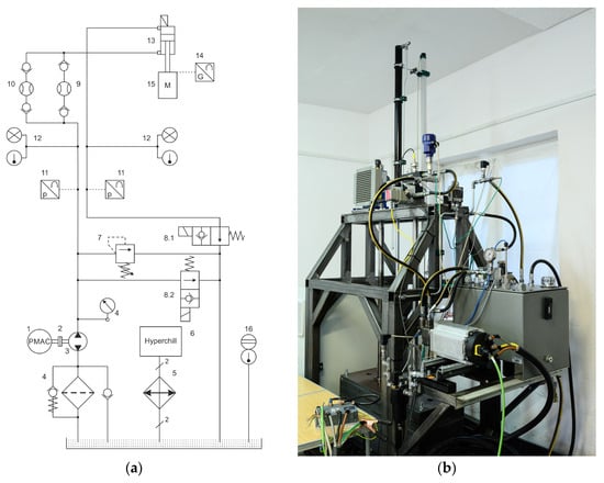
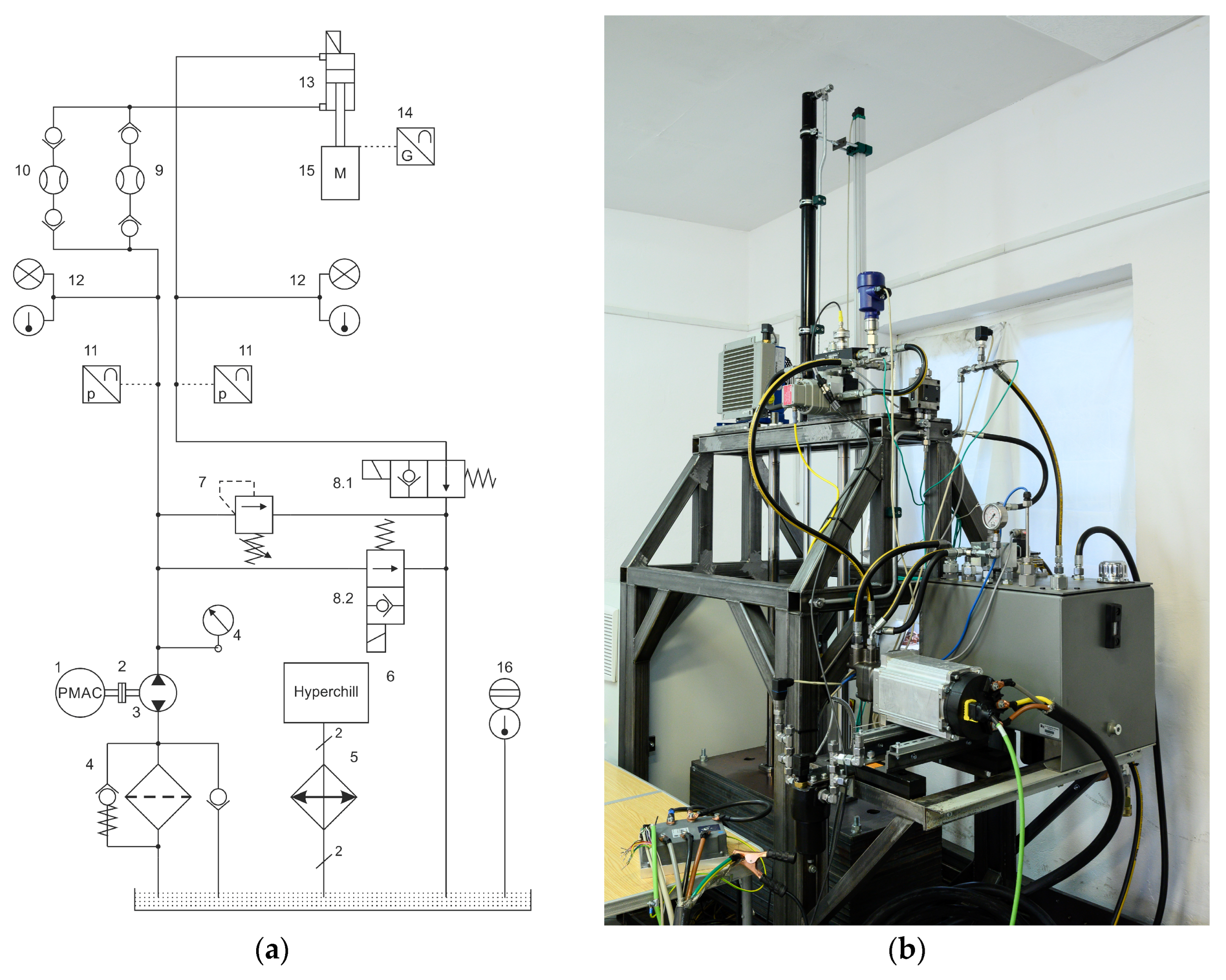
The schematic view of the electro-hydraulic test bench system with energy recuperation used in the press drive assembly is shown in Figure 1a, and the general view in Figure 1b. The bench comprises a power supply section, which includes a PMAC 1 synchronous motor with permanent magnet excitation (Parker Hannifin Manufacturing Poland, Siechnice, Poland, AC Servomotor, PN = 7.57 kW, UN = 24 VDC, IN = 342 A, TN = 35.6 Nm, nN = 2030 rpm) powered by a GVI 24 V inverter connected to a set of AGM gel batteries (Parker, 69N21107C04x01). The PMAC motor is connected via a clutch assembly 2 to a double-acting multi-piston pump 3 with a chamber volume of 5 cm3/rev. The discharge line includes a filter assembly 4 with a safety check valve and an overflow valve 7, as well as safety shutoff valves 8.1 and 8.2 controlled by a digital signal (all listed—Parker). The oil tank contains a digital level and temperature sensor 16 and a breather valve that prevents uncontrolled pressure buildup in the tank. The operating section of the station includes a hydraulic cylinder 13 (diameters: piston 40 mm, piston rod 25 mm, working length 1000 mm) with a bearing-mounted mass assembly 15 (m = 980 kg). The measuring section includes temperature probes with a current signal 12 and pressure transducers 11 (Parker, 0–250 bar), and a resistive measuring actuator ruler 14 (LCF 1250 with a 1250 mm stroke and a 4–20 mA current signal). Two flowmeters 9 and 10 were used to measure the working medium flow: the VSE VS 0.2 GPO 12V-32N11/4 0-15 lpm flowmeter with the VSE FU252 transducer for lifting (VSE Volumentechnik GmbH, Neuenrade, Germany) and the SCFTT-150-C2-05 flowmeter (Parker, Siechnice, Poland) with a measurement range from 5 to 150 lpm for recuperation algorithm. All transducers and measurement sensors were selected based on the test bench mechanical operational limits.
Figure 1.
Test bench with volumetric control method: (a) hydraulic connection scheme, (b) general view of test bench.
Based on a detailed analysis and knowledge of the rig’s parameters, its limit values can be determined. Based on the mechanical design, the maximum driving force of the piston rod can be determined, taking into account the lift height, which in this case is 9613.8 N. Furthermore, laboratory tests of the actuator’s viscous friction coefficient and oil viscosity (assumed 4.498 Pa·s, at 40 °C) were carried out. It was also possible to determine the maximum steady-state speed of the actuator–mass system, amounting to 3.02 m/s. In this case, achieving maximum values on the rig is not permissible due to the design and technological limitations of the components used. The additional parameters determined through synthesis during the rig’s construction are interesting: the volume of fluid accumulated in the actuator (842.34 cm3), which drives the hydraulic motor–electric motor system during energy recuperation with maximal flow rate at 120 lpm, and the balance of gravity of the actuator–mass assembly and piston rod resistance at system pressures above 125 bar.
The control and measurement system was implemented on a PLC (Beckhoff, CX 2033, Beckhoff Automation, Verl, Germany), and to measure the required values for the control system, EL 3124 measurement cards for current signals of 4–20 mA and voltage signals of ±10 V, and EL 3014 and ELX 3314 for thermocouple measurements were used.
The measurement uncertainty of the electrical and hydraulic quantities used to calculate the power consumed or recovered within the control system was also estimated. The low-voltage GVI inverter employed utilizes Field-Oriented Control (FOC), which offers high control accuracy—on the order of 0.02%—though it requires feedback on the rotor position of the PMAC motor. The calculation of the combined type B instrumental uncertainty for electrical and hydraulic power accounts for measurement errors within the control and monitoring system, specifically involving the input/output modules of the Beckhoff PLC. Voltage and current data from the GVI inverter are acquired via a CAN interface, with an associated uncertainty of ±1.45 W. These measured values were compared against readings from an external UNI-T UT203R clamp meter (Uni-Trend Technology (China) Co., Ltd., Dongguan, China), which has a measurement uncertainty of 7 W. Across several verification experiments, the electrical power measurements remained consistent, despite the differing uncertainties of the external clamp meter and the inverter’s internal measurement system. For hydraulic power (33), the measurement uncertainty associated with the sensors used is ±1.13 W. Consequently, it can be concluded that the experiments were characterized by very low measurement uncertainty, and the results obtained are highly reliable. All sensor sampling times were the same, equal to 1 ms.
3. Optimization Control Algorithm
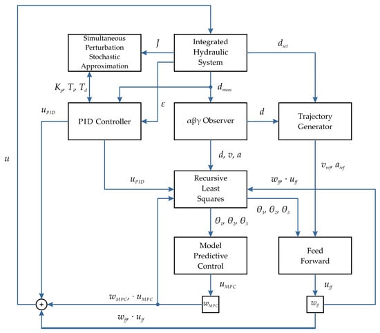
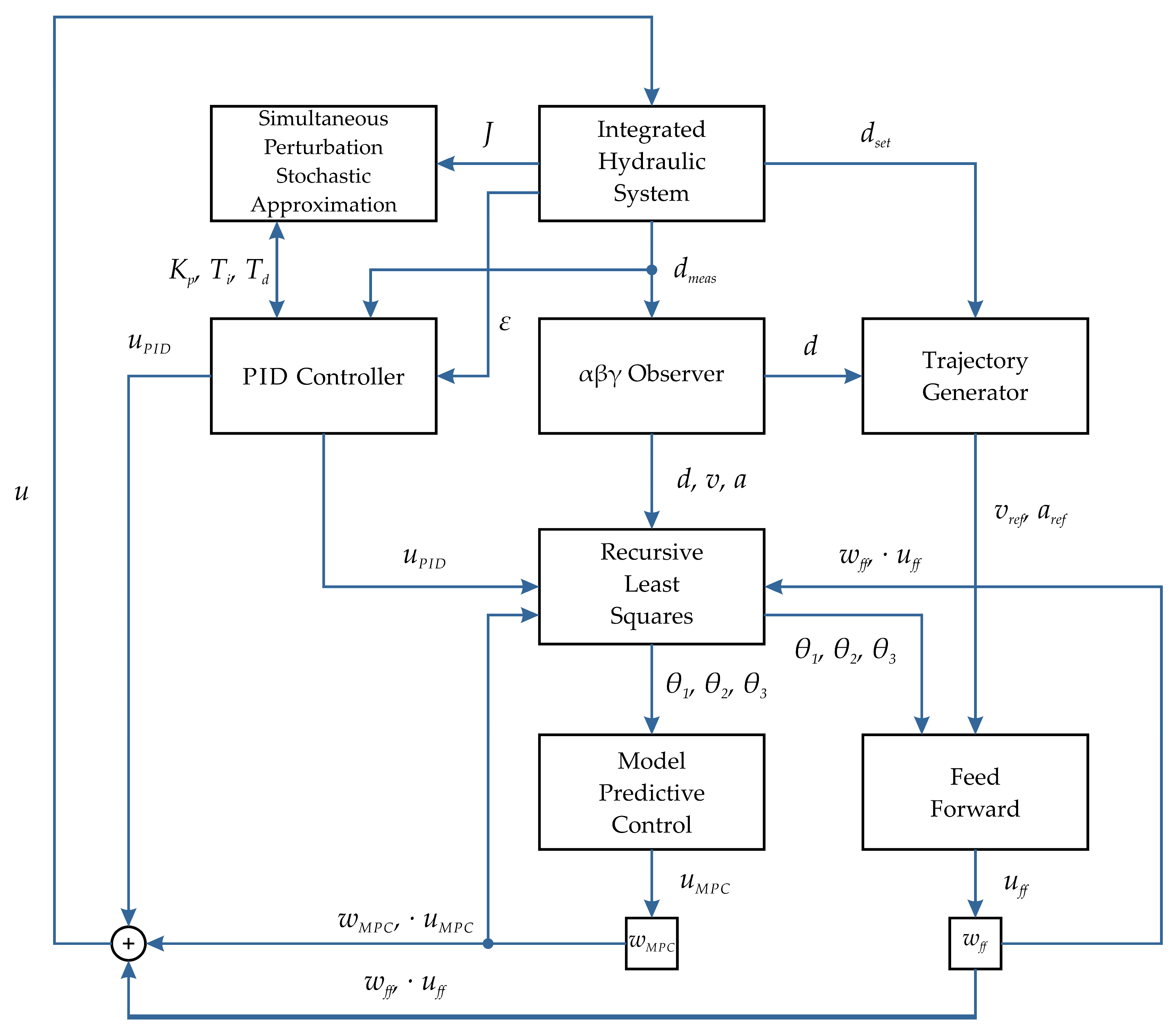
The control optimization solution proposed in this paper was developed to maximize the energy efficiency of an electro-hydraulic drive system with volumetric control and simultaneous energy recovery, while maintaining high positioning accuracy and insensitivity to changing operating conditions. Unlike many of the methods described, which primarily focus on a single control aspect, such as reducing control error, the presented system integrates several complementary control methods into a single unified architecture, as shown in Figure 2.
Figure 2.
The block diagram of the adaptive optimization algorithm.
The basic assumption of the proposed solution is the continuous adaptation to changes in the dynamics of hydraulic drive operation. Under such conditions, the use of a controller with fixed settings would lead to a progressive deterioration of the control quality of the system. To counteract these factors, a multi-layer adaptive control structure was developed. Each layer of the presented solution is used to perform a different task within the control system, and as a whole, they cooperate by exchanging state variables and identified system model parameters. The system’s layered architecture and clear separation of individual functions allow for easy implementation of the solution, even in PLCs, which is particularly important due to the possibility of applying the solution to existing hydraulic drive automation systems without the need to integrate external systems and devices.
The system has solutions that allow for compensation of rapid changes in the control object using model-based control and continuous identification of model parameters (RLS update rate is 5 ms). At the same time, it ensures optimization of the system’s operating parameters over a longer time horizon by using a setting adaptation algorithm, the operation of which is triggered every full cycle of the system’s operation (up and down load movement).
The trajectory generator is the master control system for the feed forward system. Based on the specified positional limits, a motion profile is generated with dynamics determined by defined speed and position constraints. The algorithm calculates the point at which braking must begin before the set limit is reached and subsequently—following a change in direction—executes a smooth acceleration up to the maximum speed. Due to its low computational complexity and simple implementation, a trapezoidal motion profile was chosen. Unlike polynomial trajectories, reference motion parameter values require a small number of iterations to complete the calculation. The implementation of the trapezoidal trajectory [41] is presented in Appendix A. The actuator velocity and acceleration reference values calculated from Listing A1 are then passed to the FF algorithm. The controlled object does not have devices that enable physical measurement of the speed and acceleration of the actuator during operation. The only measurement quantity available to identify the actuator’s condition is its position. For this reason, an αβγ state observer employing numerical differentiation with low-pass filtering [42]—a simplified version of the Kalman filter—was used. Due to the significant noise level in the position reading, caused by electromagnetic interference from the inverter system and other sources, the system predicts the current position and subsequently corrects it based on the signal read from the linear scale. Position estimation is determined according to the following relationships:
where dp—position prediction, v—current speed, Ts—PLC cycle time, c—difference between the measured and predicted value, da—position measured using a ruler, dt—estimated position, and α—position filtration parameter.
dp = dt + v × Ts
c = da − dp
dt = dp + (α × c)
c = da − dp
dt = dp + (α × c)
The position values are stored in a table, and a velocity estimate is calculated based on them. The velocity is calculated with use of the position value from an earlier time moment to minimize noise. In this case, the delay is 4 ms (4 controller cycles). Based on current and historical measurements, a predicted velocity value is calculated and a new velocity is calculated based on the difference between the predicted and current velocity, weighted by the β parameter:
where vp—velocity prediction, dt—current position estimate, x—velocity estimate delay, Ts—PLC cycle time, vt—estimated velocity, and β—velocity filtration parameter.
As with velocity, this algorithm is also used to estimate acceleration. To limit the impact of noise accumulation in the previous observer steps, the time constant for calculating acceleration is even greater, in this case equal to 8 ms (8 controller cycles):
where ap—acceleration prediction, vt—current velocity estimate, y—acceleration estimate delay, Ts—PLC cycle time, at—estimated acceleration, and γ—acceleration filtration parameter.
Due to the multiplication of noise in subsequent estimations, the obtained values should be filtered to remove rapidly changing signal interference. For this purpose, a low-pass filter [43] was used in the form
where yt—filtered value, δ—filtration parameter, and xt—current measurement.
yt = yt−1 + δ(xt − yt−1)
The issue of filtering estimated values is important due to online system modeling. Model parameters are calculated in real time, and signal noise can significantly affect the calculated model error, resulting in inefficient adaptation of model parameter values.
The next layer of the control system is the object dynamics model identification system. The operating parameters of the hydraulic system are not constant throughout the machine’s lifespan and are often not constant within the machine’s operating cycle. Online object modeling methods can be used to compensate for changes that occur in the system. The dynamic model equation [44] based on the equation of motion of the forces acting on the actuator was used to describe the object studied.
where m—load mass [kg], a—actuator acceleration [m/s2], Fh—hydraulic force [N], Fd—damping force [N], Fg—gravity force [N], and Fu—unmodeled forces [N].
ma = Fh − Fd − Fg − Fu
Assuming a linear damping model and a linear dependence of the hydraulic force on the control signal,
where B—viscous damping coefficient [Ns/m], v—velocity [m/s], Ku—proportionality coefficient of the control signal to the force [N/rpm], and u—control [rpm]; substituting the values into Equation (5) we obtain the expression
and after dividing by the load mass we obtain
Fd = Bv
Fh = Kuu
Fh = Kuu
ma = Kuu − Bv − mg − Fu
Entering parameters
the resulting equation takes the form
where a—acceleration, u—control signal, v—velocity, θ1—control coefficient, θ2—damping coefficient, and θ3—gravity and unmodeled effects.
a = θ1u − θ2v + θ3
The given control model was used as a regressor in the Regressive Least Squares (RLS) algorithm [45]. The implemented algorithm is an algorithm with a forgetting function implemented by the parameter λ satisfying the condition 0 < λ < 1. The use of the forgetting coefficient causes an exponential “memory decay” with respect to historical results, which allows for modeling the current system, regardless of its previous state. The regression vector takes the form
Based on the parameters θ1, θ2, θ3 calculated in the previous iteration of the algorithm, the prediction is determined in the form
and based on it the model error
where y—estimated actuator acceleration.
The adaptation coefficient is updated according to the equation
where Pk—covariance matrix, φk—current regressor, and λ—forgetting coefficient, and the model parameters are updated according to the formula
where θk—vector of model parameters, and ek—model error.
θk = θk−1 + Kkek
The covariance matrix is updated according to the equation
where I—identity matrix.
Unlike conventional adaptive control systems, the model is not solely used to estimate the model response, but is used as an integral part of the FF and MPC algorithms, which constitute the next layer of the architecture.
The first algorithm is the adaptive feed forward controller, which uses an algebraic inversion of the dynamics model [46] given by
where uff—control, a—reference, v—speed, and θ1, θ2, θ3—model parameters.
Its task is to control the actuator to move along the motion curve specified by the generator.
The second algorithm, MPC, uses the parameters identified by the RLS algorithm to predict future states of the system [23]. The prediction is performed over a range of n time steps, called the horizon. The predicted system responses are determined for several different control scenarios to select the candidate with the lowest cost. The position model is in the form of an equation
where xk—position in the current iteration, Ts—PLC cycle time, and vk—velocity in the current iteration, and the velocity model
where vk—predicted speed, uk—current control, and θ1, θ2, θ3—model parameters.
xk+1 = xk + Tsvk
vk+1 = vk + Ts(θ1uk − θ2vk + θ3)
At each time step, the cost function is calculated in the form
where we—error weight, e2—error square, wd—control change weight, and ∆u—difference between the current and proposed control.
JMPC = wee2 + wd(∆u)2
The cost function reduces errors relative to the setpoint and large changes in the value of the control parameter. At each time step, the output of the function is summed and after calculating the prediction for the entire range, it is compared with the lowest cost of a given algorithm iteration. If the value is less than the best cost, the control for which the prediction was made becomes the best control. If not, the control remains unchanged. After completion of the entire algorithm iteration, the control with the lowest cost is assigned to the output of the function block. Despite using the same model, both algorithms implement significantly different functions. The FF controller compensates for the system dynamics by smoothing the actuator’s motion near extreme positions, whereas the MPC controller predicts future control error and applies control corrections as countermeasures. Despite the use of model-based control, the proposed solution is based on a classic PID controller with a negative feedback loop, with additional controllers used as correction devices. Due to the asymmetric characteristics of the controlled object’s movement for up and down movements, the control system uses two independent controllers assigned to a specific direction of movement. The controllers used are described by the following equation:
where u(t)—control signal, Kp—proportional coefficient, ε(t)—control error, Ti—integration time constant, and Td—differentiation time constant.
The use of separate controllers allows for independent optimization of settings for both directions of movement, compensating for differences caused by gravity and asymmetry in the hydraulic cylinder chambers. The outputs of the PID controllers, FF controller, and MPC controller are summed, and the signal is then transmitted to the electro-hydraulic drive:
where u—control signal, uPID—PID controller output, uff—FF controller output, uMPC—MPC controller output, and wff, wMPC—control weights.
u = uPID + wffuff + wMPCuMPC
The final element of the control system is the PID controller adjustment system. Unlike model-based algorithms, adjustments are made after the actuator completes a full cycle. This allows for multi-criteria evaluation of the drive system’s performance using indicators such as control error, energy consumption, and motion oscillations. Based on the selected indicators, the cycle cost function is calculated, described by the equation
where wE, wε, wo—weights of optimization indicators, E—instantaneous energy supplied to the system, ε—absolute control error, and j—jerk.
The values are summed over the entire actuator movement cycle, separately for the up and down movements. For optimization purposes, the SPSA algorithm [35] was used, which is run after each upward–downward movement cycle—the adaptation is not performed according to the instantaneous values of the operating parameters. After each iteration, a random perturbation vector is generated in the form
Using the current controller settings, two sets of test settings are determined:
where ck is the perturbation amplitude.
K± = Kk ± ck∆k
In the next two iterations, full cycles of operation are performed with both sets of parameters and the cost function is calculated for each cycle:
J± = J(K±)
Based on the objective functions determined for both sets, the gradient of the cost function for each of the parameters is determined:
Then, using the determined gradient, the controller settings are updated according to the formula
Kk+1 = Kk − ak · gk
In order to ensure the convergence of the algorithm, after each iteration the learning step and perturbation amplitude are reduced according to the following relationships:
where a—update factor, A—stability constant, k—iteration number, α—step decay exponent, c—initial perturbation factor, and γ—perturbation decay exponent.
In order to limit sudden changes in controller settings, the ak·gk term was upper-limited for each parameter.
Table 1 summarizes all signals used in the system control algorithm.
Table 1.
Summary of all signals involved in the control structure.
4. Experimental Results of Adaptive Control
To assess the impact of the presented solution on the operation of the electro-hydraulic actuator, a series of tests were carried out on a test stand, with particular emphasis on the impact of optimization algorithms on the operation of the system according to the structure in Figure 2. The tests described below were performed in a position-based follow-up control structure. The position values were set within a range of 300 mm to 1150 mm, corresponding to the safe range of movement of the piston rod without reaching the endpoints. The position was set using a triangular ramp with a rise (and fall) time in the range of 3–7 s (fixed for each test batch). All experiments at the research station were conducted under the same work conditions, including a constant working fluid temperature of 40 °C of tolerance ±2 °C. The rotary speed of the electric motor–hydraulic pump system was changing significantly during the control cycle from zero to the nominal speed. Without load, the start voltage of the supply battery was the same, and all tests were carried out from the full charge state of the battery (25.0 V ± 0.5 V).
4.1. Experimental Setup Parameterization
To ensure reproducibility of experimental configuration parameters, starting conditions and special cases handling of used methods are described below.
4.1.1. PLC Settings
The control program and all algorithms mentioned below run within a single task with a cycle time of 1 ms. The cycle time is unexceedable; therefore, every line of code must be executed within a given time.
4.1.2. PID Controller
The PID controller is run every controller cycle. Parameters used in experiments described in Section 4.2, Section 4.3, Section 4.4 and Section 4.5 were Kp = 50, Ti = 50, Td = 0.005 for upward movement regulator and Kp = 30, Ti = 10, Td = 1 for downward movement. Parameters were manually tuned with the focus on avoiding oscillations and overshoot while maintaining repeatable trajectory tracking and possibly low tracking error.
4.1.3. αβγ State Observer
The state observer is run every controller cycle. Measured and estimated values are stored within a 64-element buffer. Parameters are estimated each cycle; velocity estimation is using historical position value from four cycles ago, and acceleration estimation is using velocity value from eight cycles ago. The values of the parameters are as follows: α—0.85; β—0.005; γ—0.0025.
4.1.4. RLS
The RLS algorithm is run every 5 ms (5 PLC cycles). The initial values of θ1, θ2, θ3 are all set to 1, and the covariance matrix Pk is initialized as the identity matrix with values all set to 1000. Values of θ1, θ2, θ3 are limited within range ±100. The forgetting factor λ is set to 0.92 for upward movement and to 0.89 for downward movement. Algorithm inputs—acceleration a, velocity v and control u—are all signed values. The control signal u is the actual value sent to the inverter, consisting of the sum of PID, FF and MPC algorithm outputs, and is limited within range from −2250 rpm to 2250 rpm.
4.1.5. FF
Feed forward is run every 5 ms (5 PLC cycles). Control restrictions are limited between −2250 rpm and 2250 rpm. Due to possibility of division by 0, based on Equation (17), the algorithm uses the previous control value in the case of θ1 = 0.
4.1.6. MPC
The MPC algorithm is run every 10 ms (10 PLC cycles). The prediction horizon of the algorithm is 50 PLC cycles (50 ms), control constrains are limited between −2250 rpm and 2250 rpm and cost function weights are ωe = 100 and ωd = 1. Each algorithm cycle’s candidate control inputs are generated based on the actual tracking error as a nine-element array:
where ek—tracking error, xset,k—setpoint value, xk—actual position, ui,k—candidate control array, BestUk—previous best control, and ωi—candidate weight.
ek = xset,k − xk
ui,k = BestUk + ωiek
ωi ∈ {−1; −0.75; −0.5; −0.25; 0; 0.25; 0.5; 0.75; 1}
ui,k = BestUk + ωiek
ωi ∈ {−1; −0.75; −0.5; −0.25; 0; 0.25; 0.5; 0.75; 1}
4.1.7. SPSA
The algorithm is run after each full cycle of upward and downward movement, which means that the full algorithm iteration is completed after three full trajectory cycles. Initial PID parameters for SPSA experiments were Kp = 50, Ti = 50, Td = 0.005 for upward movement regulator and Kp = 30, Ti = 10, Td = 1 for downward movement. Parameters adopted for learning step ak: A = 1, α = 0.602, = 1, = 0.1, = 0.1. Parameters adopted for perturbation amplitude ck: γ = 0.101, = 2.5, = 1, = 0.5. Parameters were limited within given ranges: Kp ∈ [0.1;1000], Ti ∈ [0;10,000], Td ∈ [0;10,000]. Cost function weights: wE = 1, wε = 0.6, wo = 0.6. Weights were selected based on experimental verification focused on omitting oscillations during algorithm convergence and limiting possibilities of the algorithm getting stuck in local minima. Based on experimental verification of the order of magnitude of each cost function, element parameters were normalized using given normalization parameters: energy—0.001, error—0.0001, jerk—0.01.
4.2. Online Dynamic Model Validation
The scope of the tests in this case included recorded time responses for a control system with a PID controller. Separate controller instances with individual settings were used for the up and down movements. The ramp-up time was set to 5 s in the experiment.
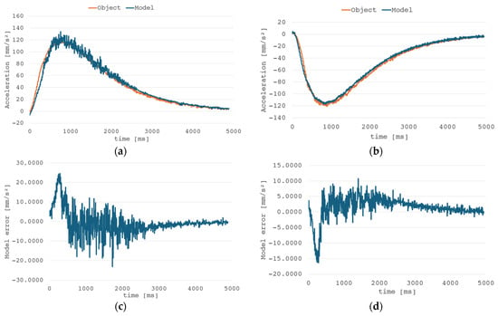
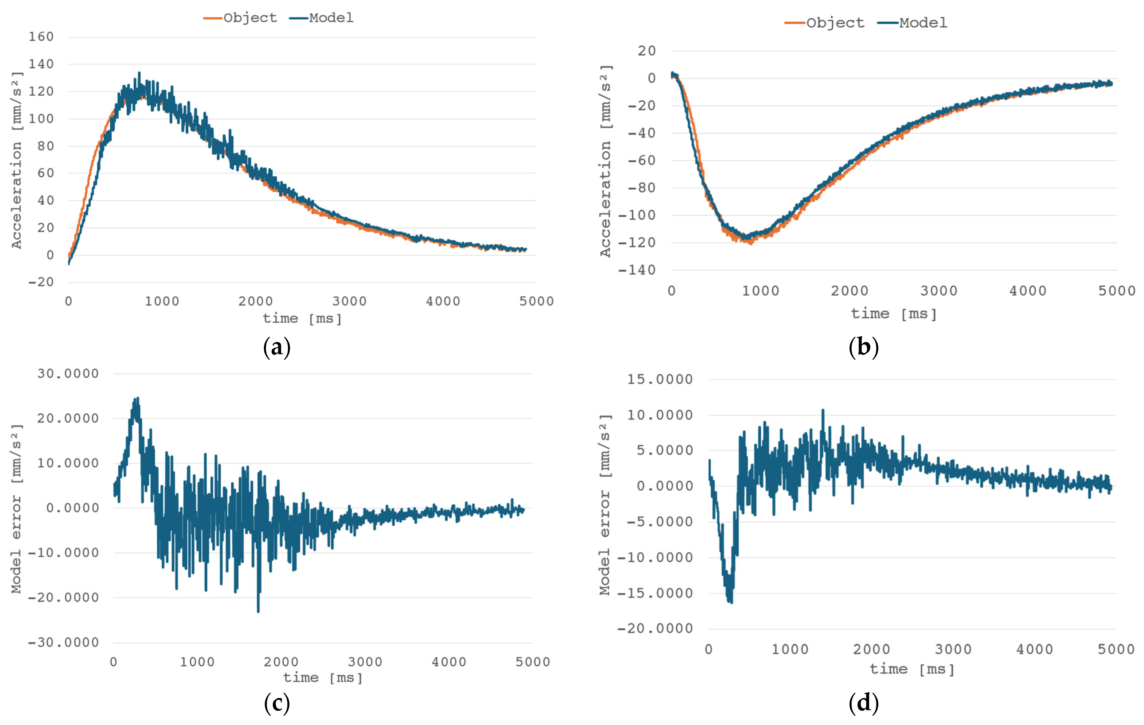
Based on the graphs in Figure 3, it is clear that the model converges for both the upward and downward motions. The mean error converges to 0, and the oscillations that occur are the result of estimator noise. Nonlinearity was also demonstrated when the actuator’s direction of motion changes. This may be due to misalignment of the guide mounting holes or the actuator itself, which also suggests that the process of changing the direction of motion is highly nonlinear. When direction is changed, the signs and dynamics of the estimated velocity and acceleration values reverse.
Figure 3.
Comparison of the RLS model and object responses: acceleration waveform—upward (a) and downward (b) movement, RLS model error—upward (c) and downward (d) movement, cycle time—5 s.
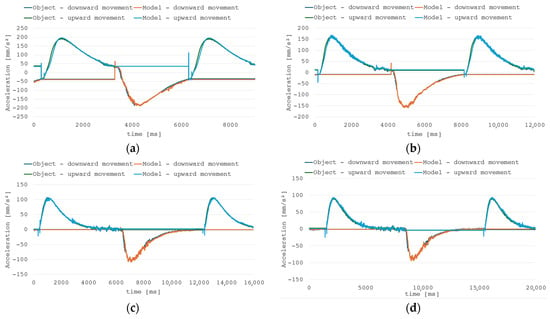
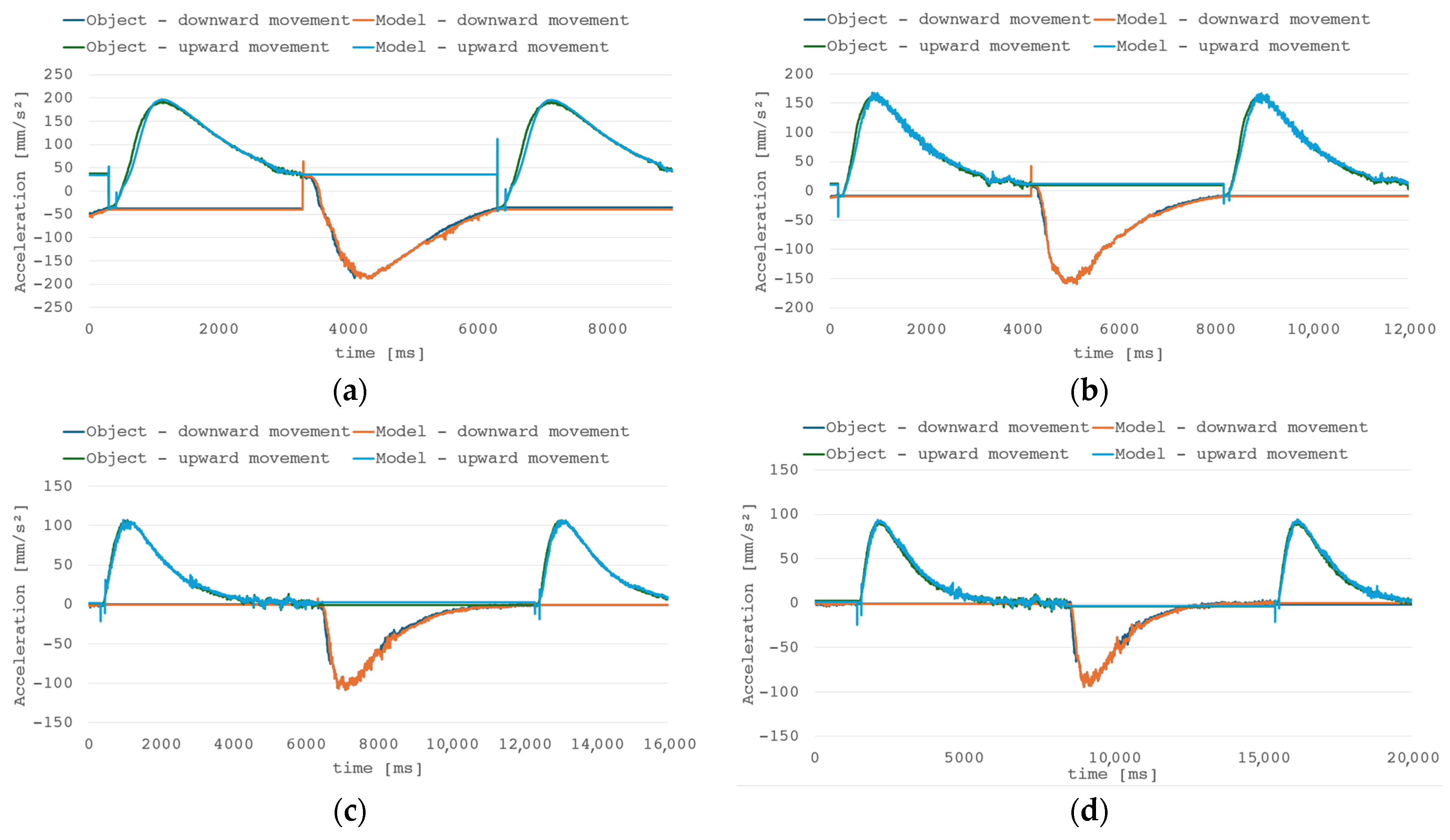
As seen in Figure 4, change in direction can cause impulsive change in model estimation, but error is quickly reduced. Due to inertia of the hydraulic system, the impact of such an event is suppressed, but it should be noted that in less inert applications introduction of model output filtration could be necessary to diminish the effect of sudden model changes on the control system.
Figure 4.
Comparison of the RLS model and object responses for different system dynamics—(a) cycle time 3 s, (b) cycle time 4 s, (c) cycle time 6 s, (d) cycle time 7 s.
4.3. Feed Forward Performance
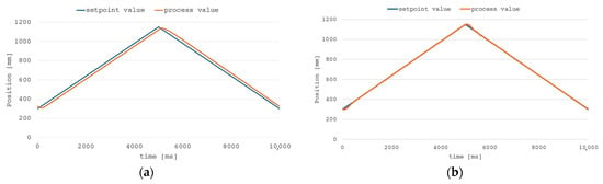
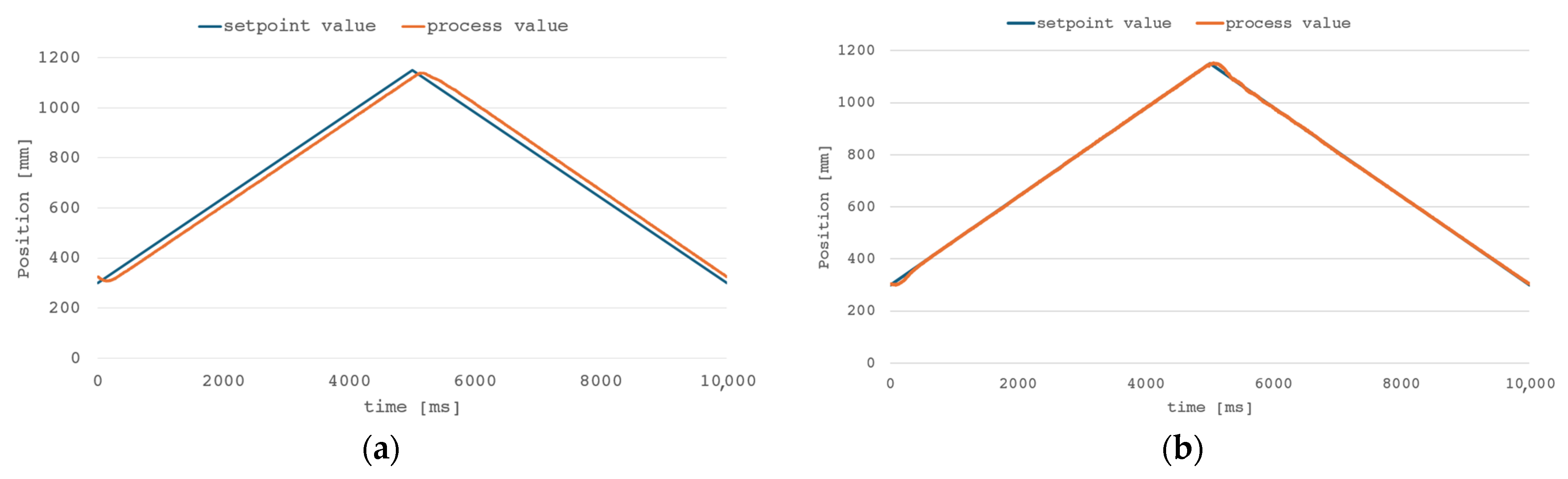
To perform a comparative analysis of the system’s operation and examine the impact of individual control system components, normal system operation and performance characteristics were determined for the control system with only a PID controller. The weight wFF of feed forward controller output is respectively 0.6 and 0.5 for upward and downward movement. The weights were manually tuned to ensure stable tracking with possibly low tracking error and overshoot. For correct control system behavior, the sum of PID controller output and weighted FF output was given as the RLS model input. Figure 5 shows the time responses of the PID control algorithm at the work cycle and after updating the control using the feed forward algorithm.
Figure 5.
Time graph of the piston rod position during the work cycle: (a) for a PID controller and (b) PID controller + FF algorithm.
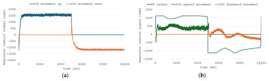
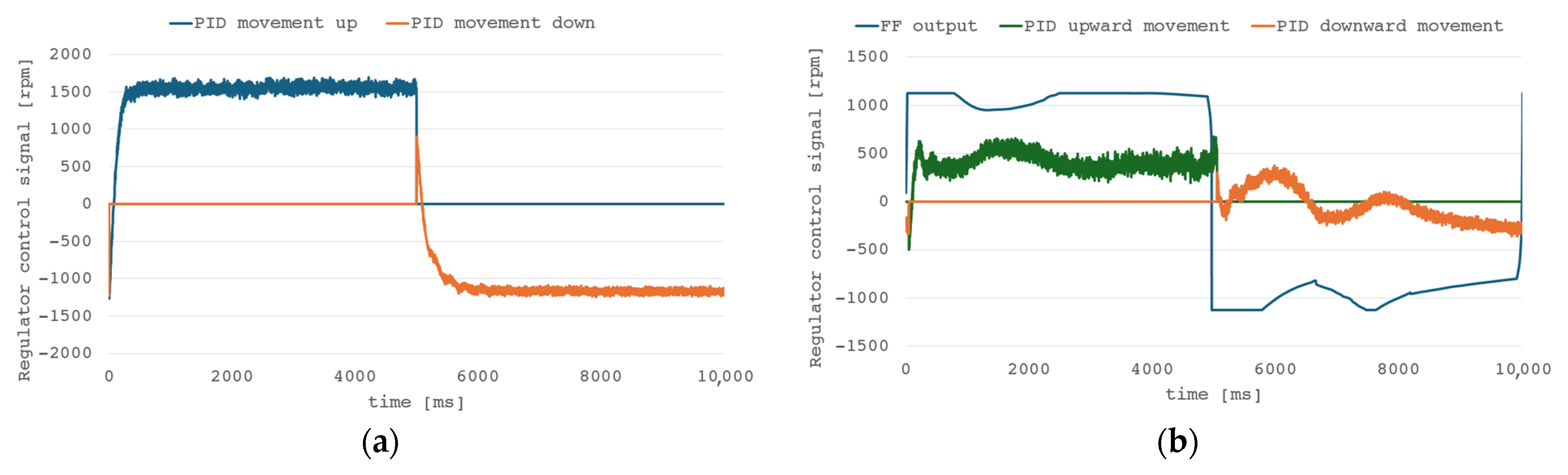
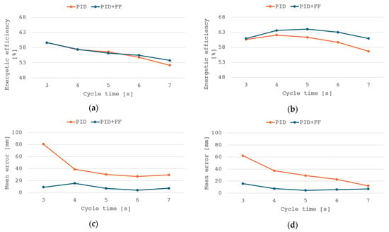
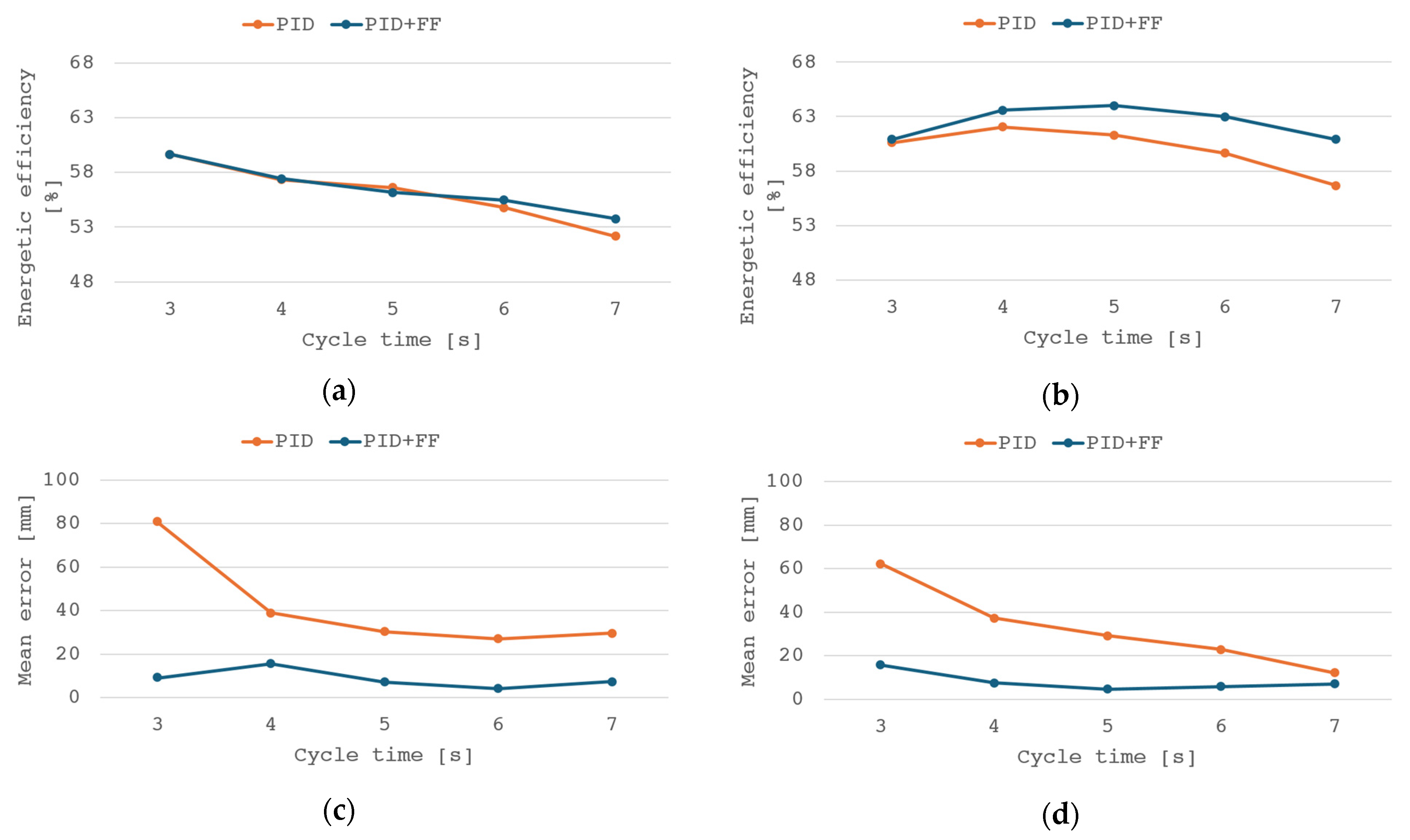
The use of an additional feed forward controller reduces the average error in the duty cycle. Additionally, the delay between trajectory and controller response is decreased, allowing the load to follow the set position with greater accuracy. Figure 6 shows the waveforms of the regulator output signals from the control system.
Figure 6.
Time responses of control signal regulator output: (a) for a PID controller and (b) PID controller + FF algorithm.
Augmented configuration reduces the control signal level of the PID controller. The feed forward controller practically takes over the primary control role, while the PID controller provides a correction to the signal, allowing it to “catch up” to the setpoint, especially around the points of direction change.
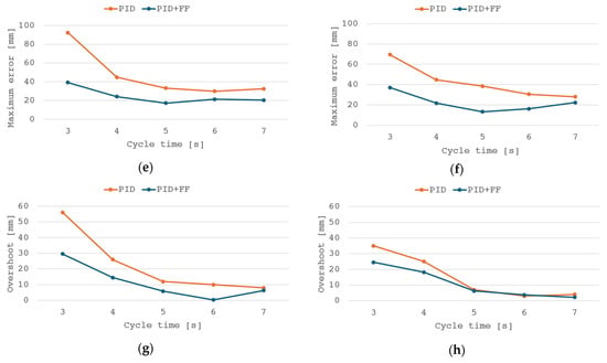
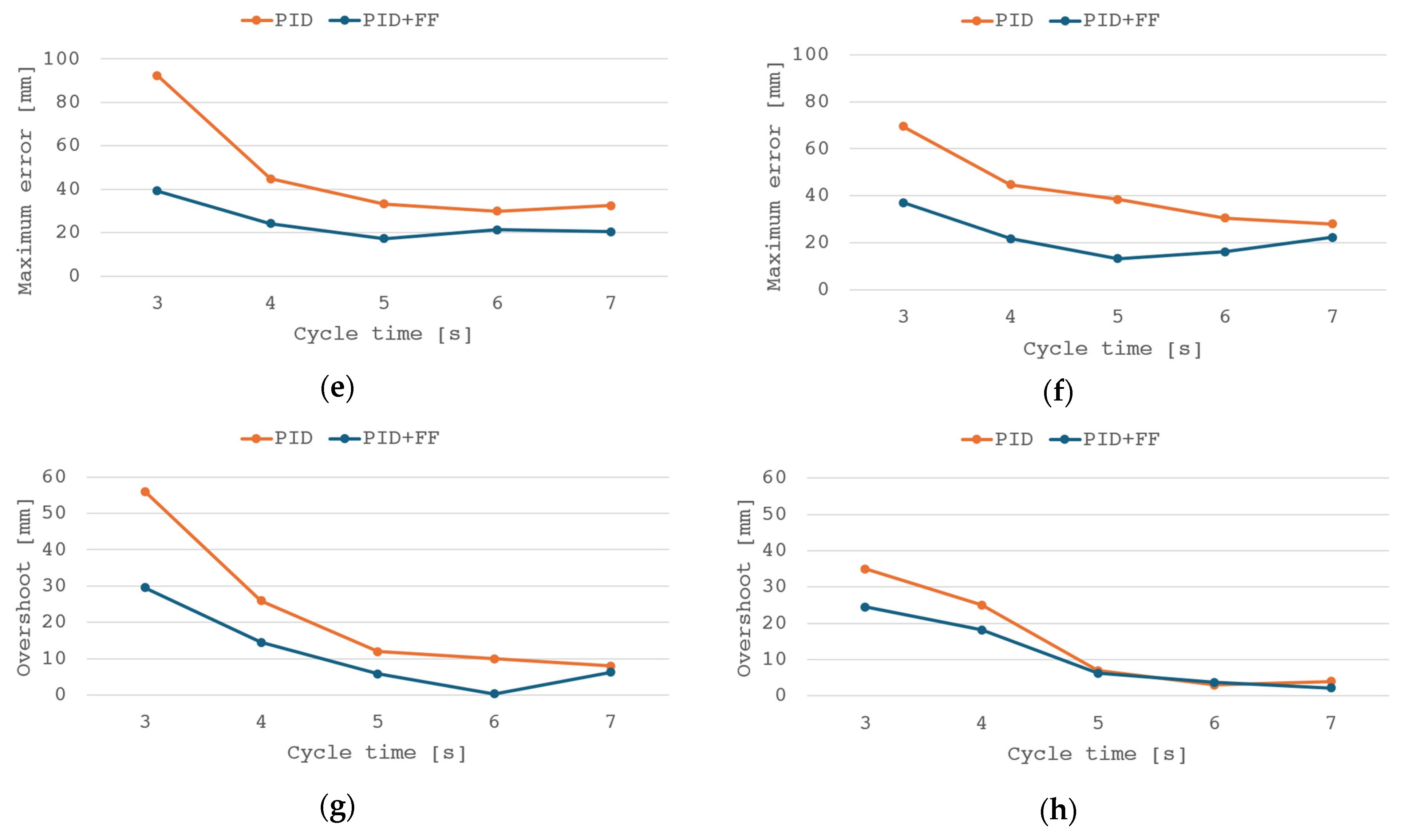
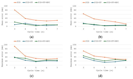
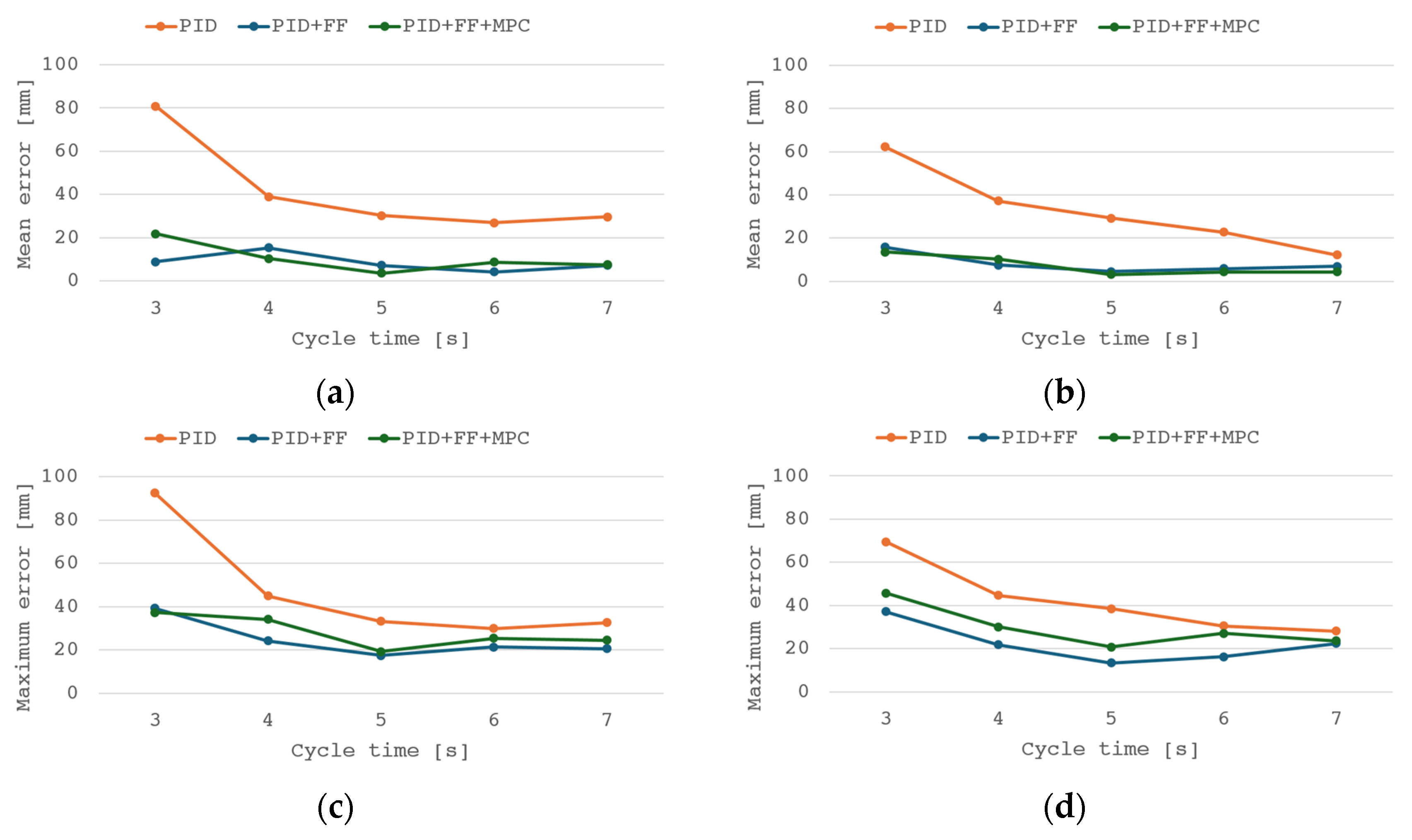
When considering the control system’s research problem in terms of energy efficiency, the feed forward controller causes a slight increase in the overall energy efficiency of the system in the case of lower-dynamics operations. Upward movement efficiency stays mostly the same as for the PID controller; however, for downward movement efficiency, the increase is noticeable. Figure 7 presents the results of the analysis of energy efficiency (a), mean control error (b), and maximum control error (c) for upward and downward movements.
Figure 7.
Analysis result graphs of: energy efficiency (a) upward and (b) downward movement, mean control error (c) upward and (d) downward movement, maximum control error (e) upward and (f) downward movement, and overshoot (g) upward and (h) downward movement.
The main advantage of the feed forward algorithm is its tracking error reduction property. The phase shift between the given trajectory and the system response is visibly reduced and the mean and maximum errors are decreased in both movement directions. Regarding mainly the follow-up function, a slight increase in energy efficiency should be noted.
4.4. Influence of Model Predictive Control
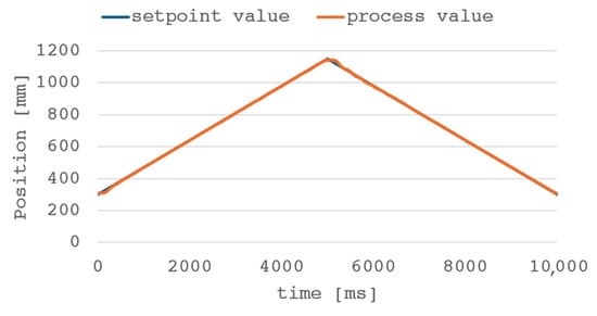
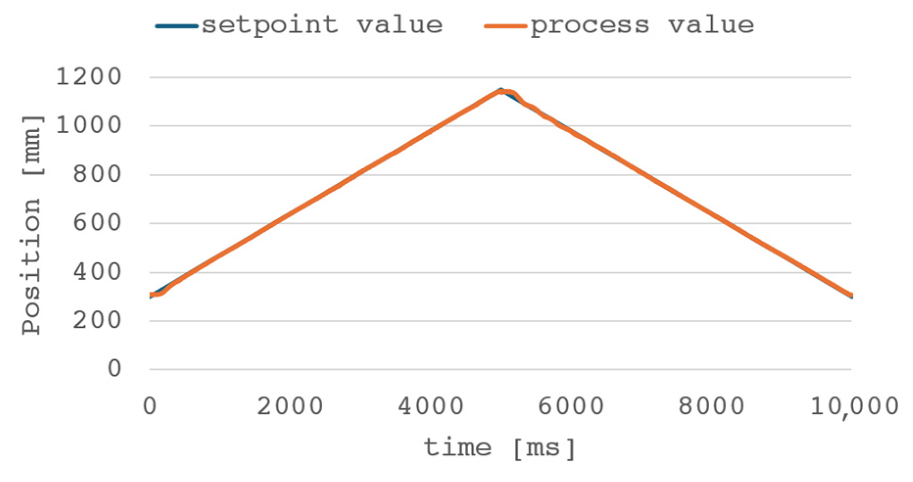
Further tests were performed using the MPC algorithm integrated into the control system. To correctly incorporate the predictive controller, the model had to include the influence of every used controller (PID, FF, and MPC). The weight wFF of the feed forward controller is set to 0.3 for both upward and downward movement, while weight wMPC is respectively 0.55 and 0.5 for upward and downward movement. The trajectory after implementing the described control system algorithm with the predictive model is shown in Figure 8.
Figure 8.
The piston rod position during the cycle with the PID + FF + MPC control algorithm.
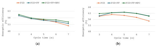
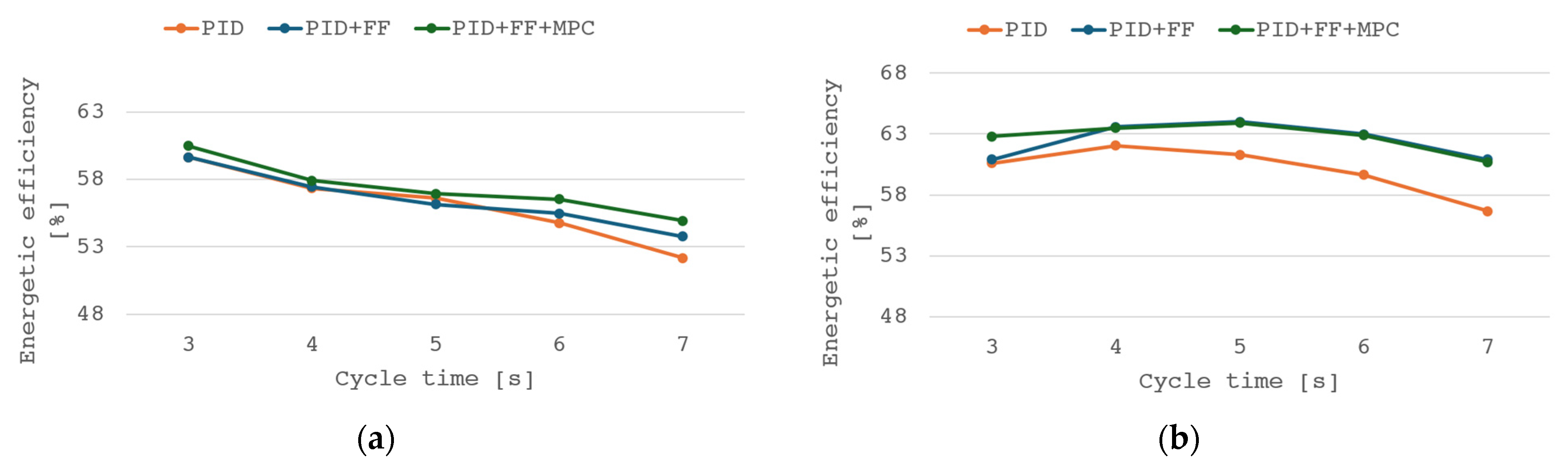
The configuration in question shows further improvement in trajectory tracking, although the appearance of a slight increase in maximum error should be noted. The introduction of an additional controller is the probable cause, as the FF trajectory tracking property could be compromised by MPC solely focused on minimizing the error. Based on results of both PID + FF and PID + FF + MPC configurations, it can be concluded that using algorithms based on the online system model allows for compensation of suboptimal PID controller starting settings. Figure 9 shows efficiency after applying control with the MPC algorithm for both upward (a) and downward (b) motion.
Figure 9.
Efficiency graphs of different control configurations for object movement: (a) up, (b) down.
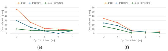
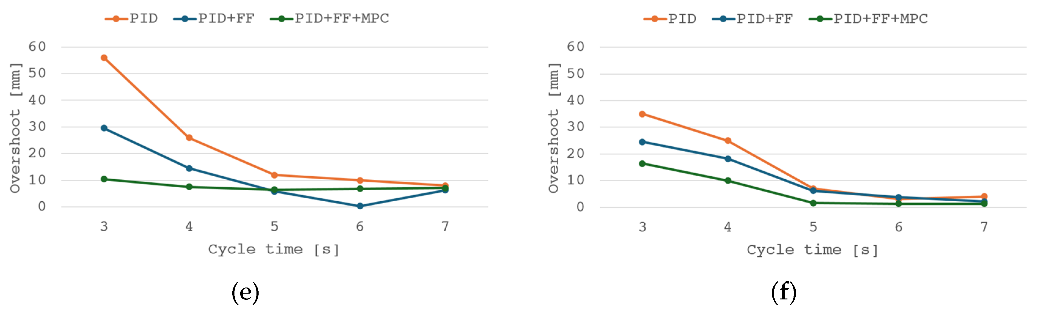
An additional advantage of the extended predictive configuration is the slight increase in energy efficiency. The PID + FF + MPC system achieves higher energy efficiency across the entire operating range, achieving a 2.7 pp. increase in the best case for upward movement and 4.0 pp. for downward movement. The results of the analysis of the mean and maximum errors of the algorithms used are summarized in Figure 10.
Figure 10.
Analysis result graphs of: control error (a) upward and (b) downward movement, maximum control error (c) upward and (d) downward movement, and overshoot (e) upward and (f) downward movement.
The tested control system configuration retains the operating characteristics of the previous controller configuration, resulting in a visible reduction in the control error at each selected operating point, although a slight increase in maximum error is present. Due to different weighing of algorithm outputs in compared configurations, determining the impact of individual algorithms should be done with particular caution. In the paper presented, emphasis is mainly placed on comparison of each augmented configuration as separate architectures. Further work might focus on presenting the impact of algorithm weights on system performance.
4.5. Energy-Oriented Adaptation
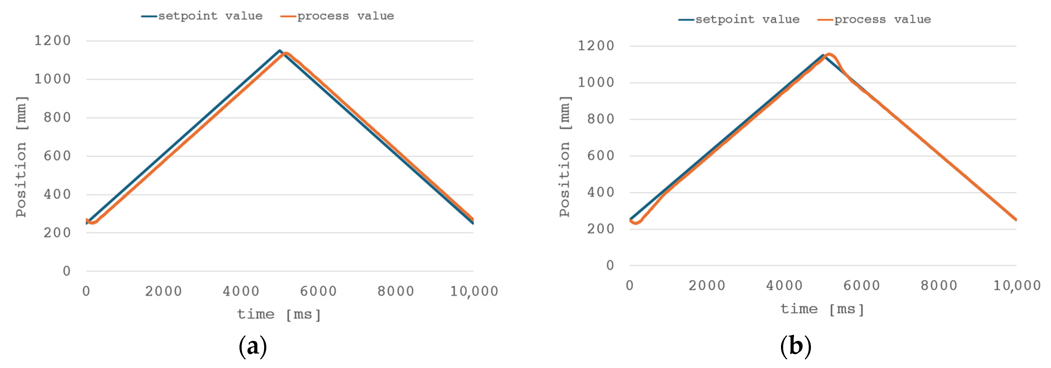
The highest level in the hierarchy of the presented control algorithm is stochastic optimization/adaptation of the PID controller parameters. To validate the solution’s performance, an adaptation system was tested for a control system with only a PID controller to exclude the influence of other algorithms. All results presented in this chapter are for a 5s cycle time. A comparison of the position trajectories before using the adaptive regulator parameters (a) and after using the SPSA algorithm (b) is shown in Figure 11.
Figure 11.
Tracking performance comparison for PID controller and SPSA algorithm: (a) PID, (b) PID + SPSA.
The applied algorithm improved the performance of the PID controller, reducing the control error during operation and increasing its dynamics; however, performance around reversal worsened. The mean error parameter for downward movement was significantly improved, reaching ~0.5 mm per full cycle. For upward movement, an improvement of 26.5% was achieved. Increase in maximum error and overshoot is a trade-off for improved tracking possibilities in phase of the transient between extreme positions. Due to significant load inertia, the simple PID controller is unable to simultaneously provide acceptable trajectory tracking and high dynamics, especially around reversal. Depending on the application and its requirements, such a trade-off could be acceptable, although in most applicable industrial cases sole use of a PID controller would not meet safety standards, lowering dynamics around extreme positions or introducing other control methods that would decrease overshoot. The adaptation process took 260 full cycles (approximately 43 min). A comparison of the used adaptive algorithms is given in Table 2.
Table 2.
Summary of the test results obtained before and after the adaptation of the controller settings.
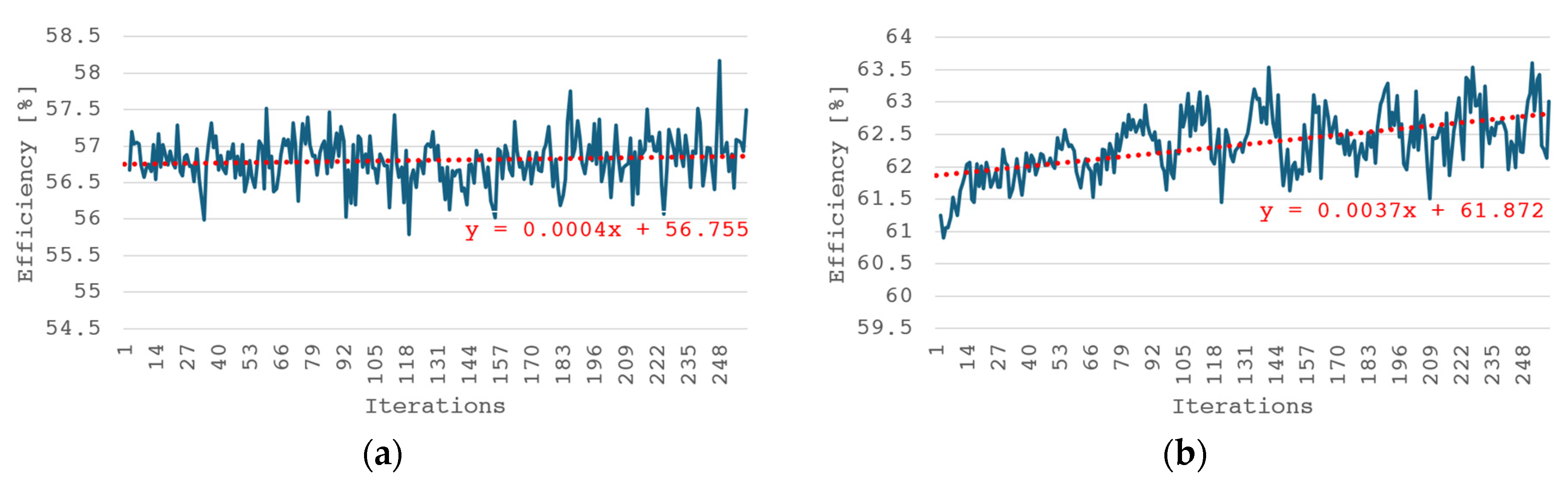
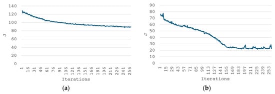
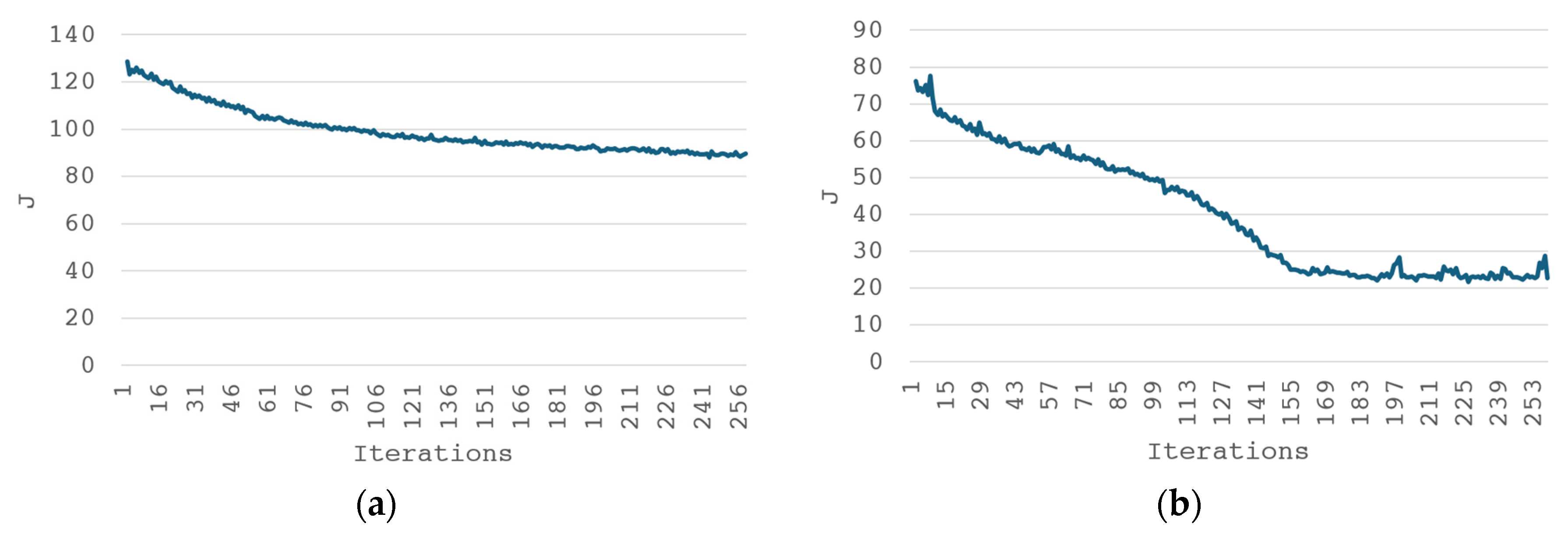
The next increasing samples in Figure 12 clearly show decreasing values of the objective function in subsequent iterations in both directions of motion. The algorithm is particularly effective in minimizing control error, which is evident when comparing the shapes of the objective function over time with the error curve for both cases. The impact of the applied algorithm on the system’s oscillations is small, but a downward trend is visible for both the upward and downward motions. In the case of optimizing the system’s energy consumption, an increase in energy is observed for the upward motion due to overshoot and therefore a longer trajectory. As presented in Figure 13 for minimization of performance index function (23), the system’s efficiency in subsequent iterations shows an increasing trend. For the downward motion, an increase in the value of recovered energy and overall energy efficiency is noticeable.
Figure 12.
Efficiency value with increasing iterations for object movement: (a) up, (b) down.
Figure 13.
Performance index change (23) with increasing iterations for object movement: (a) up, (b) down.
The analytical results obtained allow us to observe similar trends in the values of the controller settings adopted in both cases. The algorithm tends to increase the weight of the controller’s proportional term, and in the case of a low weight of the derivative term, its value also increases in subsequent iterations. For the integral term, the settings are successively reduced in subsequent cycles. In the case of a downward movement, the integral term setting is reduced practically to 0. This indicates that for optimal system tracking performance, compensating for past errors is critical, and it is far more important than predicting future errors. In context of industrial implementation, it should be noted that depending on application, the algorithm would need to be re-run with each load or dynamic change. To omit the time-consuming process of controller parameter adaptation during each change, the machine could be pre-tuned within a planned operating range and then, based on previously designated controller parameters, use the SPSA algorithm as a correction device. Attention should also be paid to possible parameter drift during long-term operation. To ensure controller stability, adaptation time should be limited to a certain cycle number/operation time with the option to recover previous “safe” parameters set in case of control parameter deterioration. Further research on optimization of control parameters should focus on determining the impact of cost function weights. The results presented in this subchapter were obtained with manually fine-tuned weights, but during the tuning process the influence of the weight ratio was noticeable, especially in the case of the presence of oscillations during the algorithm operation and getting stuck in the local minimum.
4.6. Overall Performance of the Proposed Architecture
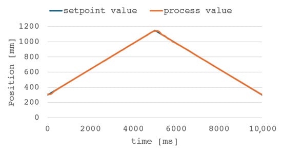
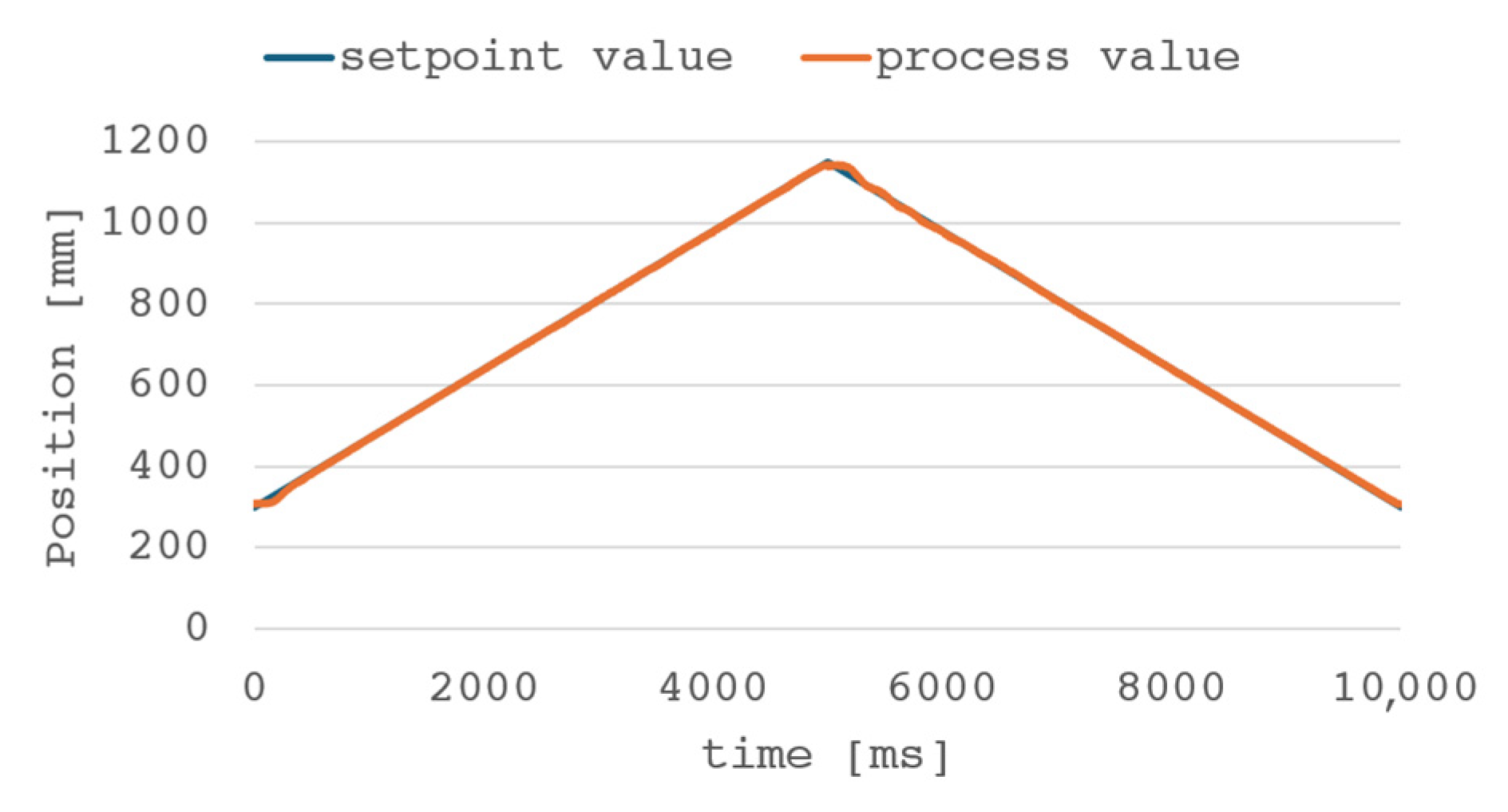
The final step in optimizing the control algorithm for the presented system is the integration of all the methods described in the previous sections. In its final form, the control system consists of a PID controller with the SPSA algorithm, a feed forward controller, and a model predictive control controller. The weight wFF is set to 0.3 for both upward and downward movement, while wMPC is respectively 0.4 and 0.3 for upward and downward movement. All results presented in this chapter are for 5 s cycle time. Figure 14 shows the time trajectory for the complete algorithm for the integrated electro-hydraulic drive control system.
Figure 14.
The piston rod position during the cycle with the PID + SPSA + FF + MPC control algorithm.
The plot shown in Figure 14 demonstrates the improved tracking performance of the control system. The system follows the trajectory throughout the cycle with low delay, and the change in direction occurs smoothly with minimal overshoot. To compare the above solution with previously described methods, the following table summarizes the experimental results.
The comparison of the control error results for the individual responses of the algorithms used is presented in Table 3.
Table 3.
Summary of the tracking errors results obtained for different control configurations.
The combination of all previously described control methods allowed for a significant improvement in the quality of regulation compared to the starting conditions. The application of the PID controller’s adjustment algorithm significantly impacted the average control error during operation. An important drawback of the proposed solution is the overshoot/delay that occurs when changing the movement direction. As mentioned in Section 4.5, it is the result of load’s inertia, and while augmenting configuration with the FF and MPC algorithms allows limiting the overshoot, its presence is still noticeable. The proposed corrector is the use of an additional indicator in the adaptation algorithm, in the form of the overshoot value. However, the specific application of the control system should be considered and the needs and constraints of the process should be taken into account when selecting the parameters of the adaptation algorithm.
4.7. Limit Values of the Energy Efficiency of the Electro-Hydraulic Actuator System
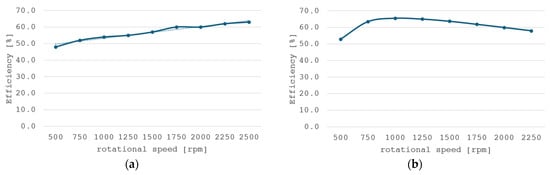
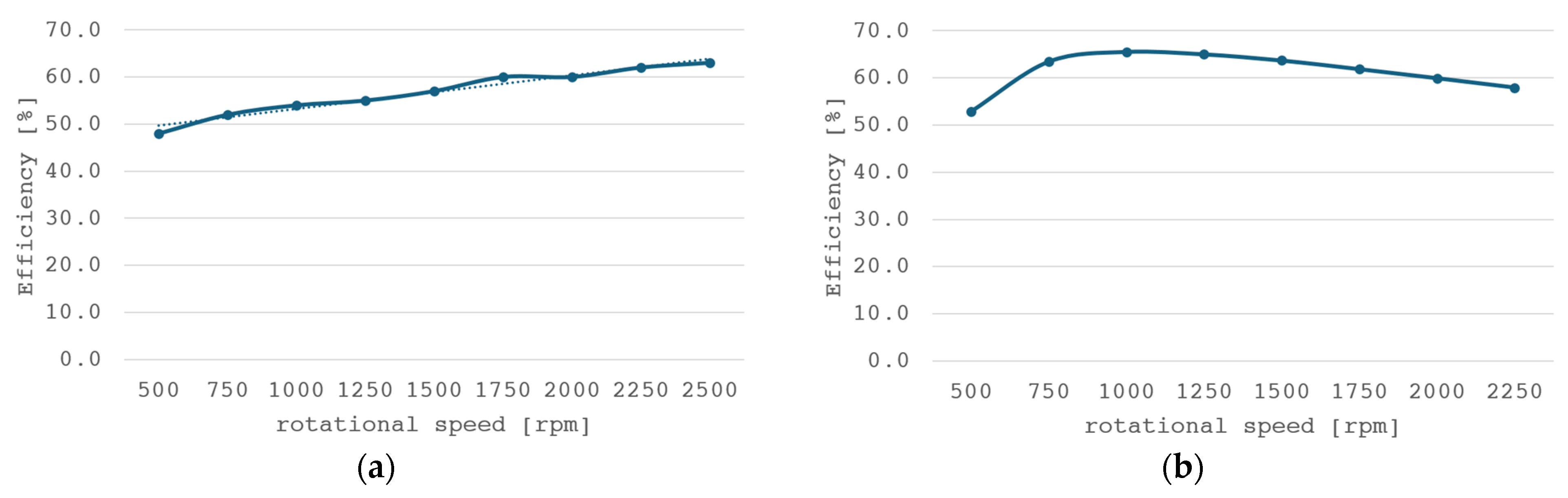
To determine the potential of the architecture of the presented control system, a study was conducted on the limits of the control system energy efficiency. During the experiments, the system had no motion limitations beyond the extreme positions of the hydraulic cylinder piston rod—the extreme positions being respectively 300 mm and 1150 mm for the upper and lower limit of rod displacement—for comparable results with previous experiments. The tests were performed with a fixed motor speed ranging from 500 to 2250 rpm with a 250 rpm step. Because the analog electric motor speed signal was used as the control signal for the system (PMAC motor–piston pump system), the study was conducted across the full functional range of the electric motor’s rotational speeds. The results of efficiency for upward and downward movement are shown in Figure 15.
Figure 15.
Efficiency for various system speeds for object movement: (a) up, (b) down.
During upward movement, the efficiency of the system increases linearly with the rotational speed of the electric motor. Consequently, higher system dynamics are expected during load lifting, allowing for a 15-percentage-point increase in efficiency at speeds approaching the rated value. During downward movement, the energy recovery efficiency varies linearly, reaching a peak at approximately 1000 rpm, where it reaches 65.5%. The energy recovery system is characterized by high efficiency, enabling the recovery of the majority of hydro-static energy across the entire range of speeds—and thus across the full dynamic range of the lifting operation.
To determine the overall energy efficiency of the electro-hydraulic drive system over an operating cycle, it is necessary to calculate the total energy supplied to the system to lift the load, the energy recovered during load lowering, and the hydraulic system energy consumed to perform the work. Efficiency is calculated as the ratio of effective hydraulic energy to net energy drain from the power supply. The overall efficiency of the integrated hydraulic drive was calculated using the formula:
where ηcycle—total cycle efficiency [%], Ehyd—hydraulic energy delivered to the load [J], Erec—electrical energy recovered by the recuperation system [J], and Eele—input electrical energy of the system, i.e., energy supplied to the input of the inverter [J]. Electrical energy delivered and recovered is measured at inverter input, so battery losses are not included within calculations. Hydraulic energy is calculated based on pressure in cylinder and hydraulic fluid flow from/to cylinder using the formula
where p—pressure in the cylinder, Q—flow from/to cylinder, and Ts—measurement time constant.
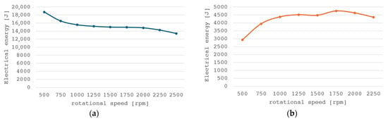
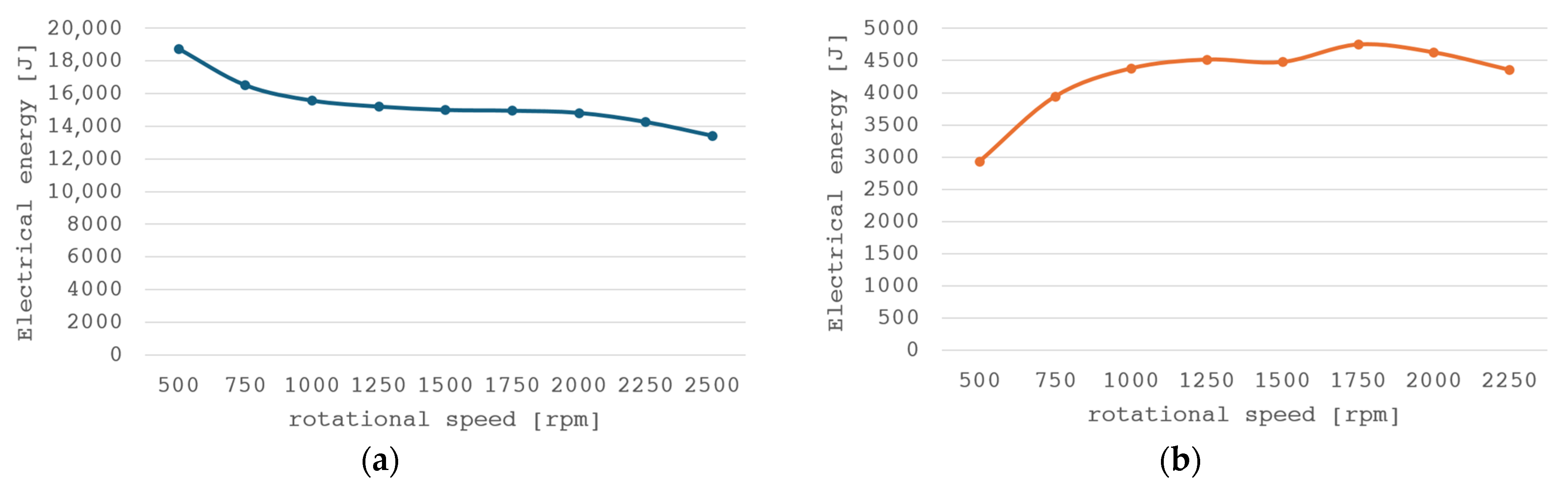
The overall electrical energy characteristics during lifting (a) and leaving the actuator as a function of rotational speed and torque are shown in Figure 16.
Figure 16.
Electrical energy consumption by the drive system: (a) energy loss during lifting and (b) energy recovery during lowering.
Based on the static characteristics with the energy values at the selected operating points shown in Figure 16, the worst-case and best-case efficiency of the integrated hydraulic system can be determined. For the worst case (lowest speed), the individual energy values are Ehyd = 8226 J, Eele = 18,747 J, Erec = 2935 J. Substituting these values into Equation (32) gives an efficiency of ηcycle = 52.0%. For the best case considered, the values are Ehyd = 8230 J, Eele = 13,442 J, Erec = 4751 J, and the calculated system efficiency value is ηcycle = 94.7%.
Given the specific nature of the problem addressed in this paper, the most critical parameter of the control system is maintaining the highest possible energy efficiency. Table 4 summarizes the efficiency of the individual systems for upward and downward motion, the overall efficiency, and the experimentally determined limit values.
Table 4.
Comparison of efficiency for selected system configurations.
As expected, among the variants presented in the control system, the system with setpoint adaptation and FF and MPC algorithms is characterized by the highest overall efficiency. Compared to the other configurations presented, a significant increase in efficiency occurs after using the SPSA algorithm. Based on this, it can be concluded that the PID controller settings have a significant impact on the energy efficiency of the test object. Inappropriate selection of settings results not only in imprecise control of the selected process variable but also in significant energy losses. Despite a limited effect on the efficiency of upward movement, feed forward and model predictive control algorithms visibly increased the overall efficiency of the cycle. Based on data shown in Figure 15, controlling drive with higher dynamics results in lower energy demand and higher energy recovery, allowing for increasing overall cycle efficiency despite the fact that the efficiency of individual movements stays approximately the same. The proposed solution, with experimentally determined best values for various system speeds, requires modification of the function to improve the system’s efficiency coefficients. The proposed implementation can be implemented cost-effectively and without modifying existing systems. The energy consumption of the system tested is summarized in Table 5.
Table 5.
Comparison of energy consumption for selected system configurations.
When comparing the absolute energy values for the various configurations, it is worth noting that as the control system is enhanced, the recovered energy values approach the best experimental value under tested conditions established for the system. This demonstrates the effectiveness of the proposed solution in optimizing control parameters to maximize energy recovery efficiency. Upward movement remains the main source of energy loss and it is in the load-lifting function that more opportunities for improving system efficiency should be sought.
5. Discussion
The presented control system solution with energy recuperation was designed with the intention of implementing it in the PLC architecture and minimal interference with the electro-hydraulic actuator’s power supply system in mind. The proposed structure requires no changes to the drive system of the facility upon implementation, but only the provision of the necessary measurement signals in the form of pressure, flow, and actuator position. Due to the widespread use of pressure and displacement measurements in hydraulic drive systems, the main cost of expanding the system would be a flowmeter.
The software portion of the solution can be implemented on any modern PLC capable of operating with a controller cycle time of less than 10 ms. External hardware or software is not required to implement the described control architecture. Due to minimal interference with the facility itself, the system may be considered to modernize existing machines such as presses, extruders, welding machines, and other vertically moving hydraulic systems. This allows for reducing the energy requirements of the machines without altering their mechanical design and adapting them to modern requirements with minimal implementation cost.
In addition to the advantages mentioned above, its limitations should also be highlighted. The results presented in this paper show that a further increase in system efficiency directly impacts the quality of the tracking. The high dynamics required to accurately follow the set trajectory simultaneously increases the system overshoot; therefore, a compromise between both tracking precision and energy efficiency must be determined depending on the application requirements. Current architecture uses fixed PID parameters and FF and MPC controller weights. In industrial use, it would be necessary to implement weight adaptation and gain scheduling for different operations to ensure safe working conditions compliant with regulations. Safety rules of the adaptation process, such as parameter change limits, gradual model impact introduction to the control system, and handling of emergency states, must be developed according to industrial standards.
6. Conclusions
The described research addressed the problem of increasing the energy efficiency of an electro-hydraulic drive system by applying the discussed adaptive control and optimization methodology. Experimental testing demonstrated a system efficiency of 94.7%, although using classical control methods with a PID controller resulted in significantly lower efficiency of 82.4%. A multi-layer control system architecture was developed that combines state variable estimation, online model identification, a model-based feed-forward trajectory controller, a predictive MPC controller, and multi-objective optimization using the SPSA method. The presented solution allows for compensation of rapid dynamic changes in the system using model-based control, while simultaneously adapting the system using stochastic optimization methods to reduce long-term energy consumption. The entire architecture is meant to be implemented on a PLC.
The presented test results demonstrated the convergence of the identified model with the test object’s responses for different dynamics, control error reduction properties using PID + FF combination, further tracking improvement and increase in energy efficiency augmenting configuration with MPC, and a significant impact of multi-criteria optimization on the energy efficiency of the drive system. The application of all the described methods allowed us to achieve an overall system efficiency of 87.9%, representing 44.7% of the available efficiency reserve compared to the classic PID algorithm. For downward motion, the system approached the experimentally obtained best energy recovery values in the tested system.
A significant advantage of the system is that the efficiency improvement was achieved using solely software methods, without the need to interfere with the mechanical part of the drive system. Therefore, the solution could be considered for implementation in both new machines and retrofitting existing systems.
The further development of the presented research direction should be based on the optimization of the weight lifting process due to the energy reserve visible in the results. Potential methods to consider include expanding the identified model to include pressure and nonlinear effects such as friction. The performance of the proposed control system architecture should also be verified in other applications, such as mobile machines or multi-axis hydraulic systems.
The results obtained clearly indicate the importance of adaptation and optimization methods as a source of improving the efficiency of electro-hydraulic drives. These methods, rather than mechanical interventions in the structure of hydraulic systems, should be considered as solutions to future problems. In this context, multi-layer adaptive architecture represents a promising direction for the development of a new generation of energy-efficient electro-hydraulic drives.
Author Contributions
Conceptualization, A.D. and W.F.; methodology, A.D. and Ł.Z.; software, A.D.; validation, A.D., W.F. and Ł.Z.; formal analysis, A.D. and Ł.Z.; investigation, A.D. and Ł.Z.; resources, A.D. and W.F.; data curation, A.D.; writing—original draft preparation, A.D.; writing—review and editing, A.D., W.F. and Ł.Z.; visualization, A.D. and Ł.Z.; supervision, A.D.; project administration, A.D.; funding acquisition, A.D., W.F. and Ł.Z. All authors have read and agreed to the published version of the manuscript.
Funding
This research was funded by Ministry of Science and Higher Education of the Republic of Poland, during the Implementation Doctorate Edition V, DWD/5/0252/2021.
Data Availability Statement
The original contributions presented in the study are included in the article; further inquiries can be directed to the corresponding author.
Acknowledgments
During the preparation of this manuscript/study, the authors used Writefull for Word for the purposes of language proofreading. The authors have reviewed and edited the output and take full responsibility for the content of this publication.
Conflicts of Interest
The authors declare no conflicts of interest.
Abbreviations
The following abbreviations are used in this manuscript:
| FF | Feed Forward |
| GS | Gain Scheduling Control |
| LQC | Linear Quadratic Controller |
| MPC | Model Predictive Control |
| MRAC | Model Reference Adaptive Control |
| PID | Proportional–Integral–Differential Controller |
| PLC | Programmable Logic Controller |
| PMAC | Permanent Magnet Alternating Current Motor |
| RLS | Recursive Least Squares |
| SPSA | Simultaneous Perturbation Stochastic Approximation |
| STC | Self-Tuning Control |
| VSVD | Variable Speed Variable Displacement |
Appendix A
The implementation of the trapezoidal motion excitation signal in the ST structured language is shown in Listing A1.
| Listing A1. The algorithm of the motion excitation trapezoidal trajectory signal. |
| VAR_INPUT Enable: BOOL; ActPos: REAL; // Actual position TargetPos: REAL; // Target Position MaxVelocity: REAL; // Maximum velocity MaxAcc: REAL; // Maximum acceleration Ts: REAL; // PLC Task time END_VAR VAR_OUTPUT PosRef: REAL; // Reference position VelRef: REAL; // Reference velocity AccRef: REAL; // Reference acceleration END_VAR VAR DistRemaining: REAL; // Difference between actual and target position Dir: REAL; // Direction of movement BrakingDist: REAL; // Calculated distance to start braking END_VAR IF TargetPos > ActPos THEN Dir: = 1; ELSE Dir: =−1; END_IF DistRemaining: = ABS(TargetPos − ActPos); IF ABS(VelRef) < MaxVelocity THEN AccRef: =Dir * MaxAcc; ELSE AccRef: =0; END_IF BrakingDist: = (VelRef * VelRef)/(2.0 * MaxAcc); IF DistRemaining ≤ BrakingDist THEN AccRef: =−1.0 * Dir * MaxAcc; END_IF VelRef: =VelRef + (AccRef * Ts); VelRef: =LIMIT(−1.0 * MaxVelocity, VelRef, MaxVelocity); PosRef: =PosRef + (VelRef * Ts); |
References
- Benić, J.; Brezak, D.; Šitum, Ž.; Kolar, D.; Lisjak, D. Detailed experimental comparison of energy efficiency between proportional and direct driven hydraulic system. Results Eng. 2023, 18, 101178. [Google Scholar] [CrossRef] [Scilit]
- Zhao, W.; Ebbesen, M.K.; Hansen, M.R.; Andersen, T.O. Experimental assessment of energy consumption: A comparative study between motor-controlled and valve-controlled cylinders in knuckle boom crane operations. Front. Mech. Eng. 2025, 11, 1535120. [Google Scholar] [CrossRef] [Scilit]
- He, A.; Wei, L.; Lu, Q.; He, P. An Investigation of Energy Consumption Characteristics of the Pump-Control System for Electric Excavator Arms. Appl. Sci. 2024, 14, 10791. [Google Scholar] [CrossRef] [Scilit]
- Hagen, D.; Padovani, D.; Choux, M. A Comparison Study of a Novel Self-Contained Electro-Hydraulic Cylinder versus a Conventional Valve-Controlled Actuator—Part 2: Energy Efficiency. Actuators 2019, 8, 78. [Google Scholar] [CrossRef] [Scilit]
- Stawinski, L.; Skowronska, J.; Kosucki, A. Energy Efficiency and Limitations of the Methods of Controlling the Hydraulic Cylinder Piston Rod under Various Load Conditions. Energies 2021, 14, 7973. [Google Scholar] [CrossRef] [Scilit]
- Zawarczyński, Ł.; Stefański, T. Efficiency Analysis of Electrohydraulic Drive with Volumetric and Throttling Control. TTS Tech. Transp. Szyn. 2013, 10, 1787–1796. [Google Scholar]
- Isidro, I.A.; Pais, D.A.M.; Alves, P.M.; Carrondo, M.J.T. Online Control Strategies. In Comprehensive Biotechnology; Elsevier: Amsterdam, The Netherlands, 2019; pp. 943–951. [Google Scholar] [CrossRef] [Scilit]
- Fister, D.; Fister, I.; Fister, I.; Šafarič, R. Parameter tuning of PID controller with reactive nature-inspired algorithms. Rob. Auton. Syst. 2016, 84, 64–75. [Google Scholar] [CrossRef] [Scilit]
- Fan, J.; Ling, D.; Tang, Z.; Pei, Z. Study on nonlinear PID control for electro-hydrostatic actuator. In Proceedings of 2014 IEEE Chinese Guidance, Navigation and Control Conference; IEEE: New York, NY, USA, 2014; pp. 1317–1320. [Google Scholar] [CrossRef] [Scilit]
- Aly, A.A. Model Reference PID Control of an Electro-hydraulic Drive. Int. J. Intell. Syst. Appl. 2012, 4, 24–32. [Google Scholar] [CrossRef] [Scilit]
- Zuo, X.; Liu, J.; Wang, X.; Liang, H. Adaptive PID and Model Reference Adaptive Control Switch Controller for Nonlinear Hydraulic Actuator. Math. Probl. Eng. 2017, 2017, 6970146. [Google Scholar] [CrossRef] [Scilit]
- Ishak, N.; Tajjudin, M.; Adnan, R.; Ismail, H.; Sam, Y.M. Real-time application of self-tuning PID in electro-hydraulic actuator. In 2011 IEEE International Conference on Control System, Computing and Engineering; IEEE: New York, NY, USA, 2011; pp. 364–368. [Google Scholar] [CrossRef] [Scilit]
- Ghosh, B.B.; Sarkar, B.K.; Saha, R. Realtime performance analysis of different combinations of fuzzy–PID and bias controllers for a two degree of freedom electrohydraulic parallel manipulator. Robot. Comput. Integr. Manuf. 2015, 34, 62–69. [Google Scholar] [CrossRef] [Scilit]
- Fan, Y.; Shao, J.; Sun, G. Optimized PID Controller Based on Beetle Antennae Search Algorithm for Electro-Hydraulic Position Servo Control System. Sensors 2019, 19, 2727. [Google Scholar] [CrossRef] [Scilit] [PubMed]
- Micheal, J.; Rahmat, M.F.; Wahab, N.A.; Lai, W.K. Feed Forward Linear Quadratic Controller Design for An Industrial Electro Hydraulic Actuator System with Servo Valve. Int. J. Smart Sens. Intell. Syst. 2013, 6, 154–170. [Google Scholar] [CrossRef] [Scilit]
- Lee, K.H.; Baek, S.G.; Koo, J.C. Real-Time High Bandwidth Feedforward Position Control of Electro-Hydraulic Actuator Using Non-Minimum Phase Inverse Model. In Proceedings of the 13th ASME/IEEE International Conference on Mechatronic and Embedded Systems and Applications; American Society of Mechanical Engineers: New York, NY, USA, 2017; Volume 9. [Google Scholar] [CrossRef] [Scilit]
- Dai, J.; Xu, H.; Si, L.; Wei, D.; Gu, J.; Chen, H. Research on Feedforward-Feedback Composite Anti-Disturbance Control of Electro-Hydraulic Proportional System Based on Dead Zone Compensation. Machines 2024, 12, 855. [Google Scholar] [CrossRef] [Scilit]
- Haas, R.; Lukachev, E. Optimal feed-forward control of a digital hydraulic drive. Proc. Inst. Mech. Eng. Part I J. Syst. Control Eng. 2017, 231, 94–106. [Google Scholar] [CrossRef] [Scilit]
- Ghazali, R.; Sam, Y.M.; Fua’ad Rahmat, M.; Zulfatman. Open-loop and closed-loop recursive identification of an electro-hydraulic actuator system. In Proceedings of the 2010 IEEE Conference on Robotics, Automation and Mechatronics; IEEE: New York, NY, USA, 2010; pp. 285–290. [Google Scholar] [CrossRef] [Scilit]
- Ghazali, R.; Sam, Y.M.; Rahmat, M.F.; Zulfatman. On-line identification of an electro-hydraulic system using recursive least square. In Proceedings of the 2009 IEEE Student Conference on Research and Development (SCOReD); IEEE: New York, NY, USA, 2009; pp. 471–474. [Google Scholar] [CrossRef] [Scilit]
- Brattley, D.A.; Weaver, W.W. Adaptive PI Control Using Recursive Least Squares for Centrifugal Pump Pipeline Systems. Machines 2025, 13, 1064. [Google Scholar] [CrossRef] [Scilit]
- Nordahl, E. Adaptive Controller for Hydraulic Motor: Implementation and Evaluation of an Adaptive Control Method for Use in a Hydraulic Servo Loop in a Fire Control System Servo. 2025. Available online: https://www.diva-portal.org/smash/record.jsf?dswid=3929&pid=diva2%3A1988419 (accessed on 17 October 2026).
- Yamada, T.; Inada, R.; Ito, K. Designing a Model Predictive Controller for Displacement Control of Axial Piston Pump. Int. J. Autom. Technol. 2024, 18, 113–127. [Google Scholar] [CrossRef] [Scilit]
- Guan, Q.Q.; Zhang, H.; Yang, J. Energy management strategy for electro-hydraulic hybrid vehicles based on an STSMO-MPC motor control algorithm. J. Braz. Soc. Mech. Sci. Eng. 2026, 48, 193. [Google Scholar] [CrossRef] [Scilit]
- Khedr, O.H.; Awad, M.I.; Al-Oufy, A.K.; Maged, S.A. Optimizing power consumption and position control in an electro-hydraulic system with cylinder bypass and NN-MPC. Sci. Rep. 2024, 14, 1993. [Google Scholar] [CrossRef] [Scilit] [PubMed]
- Sendelbach, T.; Leutbecher, T. Model Predictive Control of Electro-Hydraulic Systems with Multiple Degrees of Freedom. In 14th International Fluid Power Conference; River Publishers: Gistrup, Denmark, 2024; pp. 663–673. [Google Scholar] [CrossRef] [Scilit]
- Qin, X.; Luo, Y.; Chen, S.; Chen, Y.; Han, Y. Investigation of Energy-Saving Strategy for Parallel Variable Frequency Pump System Based on Improved Differential Evolution Algorithm. Energies 2022, 15, 5360. [Google Scholar] [CrossRef] [Scilit]
- Zhao, P.; Xie, A.; Zhu, S.; Kong, L. Pressure optimization for hydraulic-electric hybrid biped robot power unit based on genetic algorithm. Sci. Rep. 2023, 13, 60. [Google Scholar] [CrossRef] [Scilit] [PubMed]
- Raduenz, H.; Ericson, L.; Uebel, K.; Heybroek, K.; Krus, P.; De Negri, V.J. Energy Management Based on Neural Networks for a Hydraulic Hybrid Wheel Loader. Int. J. Fluid Power 2022, 23, 411–432. [Google Scholar] [CrossRef] [Scilit]
- Xu, Z.; Liu, Y.; Hua, L.; Zhao, X.; Guo, W. Energy analysis and optimization of main hydraulic system in 10,000 kN fine blanking press with simulation and experimental methods. Energy Convers. Manag. 2019, 181, 143–158. [Google Scholar] [CrossRef] [Scilit]
- Spall, J. An Overview of the Simultaneous Perturbation Method for Efficient Optimization. Johns Hopkins Tech. Dig. 1998, 19, 482–492. [Google Scholar]
- Çoban, S. Optimization of PID Controllers for UAVs Using SPSA Algorithm for Enhanced Flight Performance. J. Aviat. 2025, 9, 28–33. [Google Scholar] [CrossRef] [Scilit]
- Kocamer, A.; Çoban, S. Enhancing Longitudinal Stability of Fixed-Wing UAVs A Hybrid Approach Using PID Control and SPSA Optimization under Turbulent Conditions. Osman. Korkut Ata Üniversitesi Fen. Bilim. Enstitüsü Derg. 2026, 9, 1360–1372. [Google Scholar] [CrossRef] [Scilit]
- Kong, X.; Qian, L.; Wang, Z. SPSA-based PID parameters optimization for a dual-tank liquid-level control system. In 2016 IEEE International Conference on Industrial Engineering and Engineering Management (IEEM); IEEE: New York, NY, USA, 2016; pp. 1463–1467. [Google Scholar] [CrossRef] [Scilit]
- Ahmad, M.A.; Rohani, M.A.; Ismail, R.M.T.R.; Jusof, M.F.M.; Suid, M.H.; Nasir, A.N.K. A model-free PID tuning to slosh control using simultaneous perturbation stochastic approximation. In 2015 IEEE International Conference on Control System, Computing and Engineering (ICCSCE); IEEE: New York, NY, USA, 2015; pp. 331–335. [Google Scholar] [CrossRef] [Scilit]
- Ishizuka, S.; Kajiwara, I. Online adaptive PID control for MIMO systems using simultaneous perturbation stochastic approximation. J. Adv. Mech. Des. Syst. Manuf. 2015, 9, JAMDSM0015. [Google Scholar] [CrossRef] [Scilit][Green Version]
- Shi, L.; Zhang, X.; Liu, Y.; Xiao, G.; Ibrahim, M.; Zheng, L.; Wang, T. Optimization of electrified turbocharging: Bridging the energy-drivability trade-off. Energy 2026, 360, 141522. [Google Scholar] [CrossRef] [Scilit]
- Yang, M.; Yan, G.; Zhang, Y.; Zhang, T.; Ai, C. Research on high efficiency and high dynamic optimal matching of the electro-hydraulic servo pump control system based on NSGA-II. Heliyon 2023, 9, e13805. [Google Scholar] [CrossRef] [Scilit] [PubMed]
- Ariyanto, S.R.; Warju; Abdi, F.I.; Sakti, A.M.; Arifianti, L.S.Y.; Wirawan, W.A.; Syifa’Nugraha, A. Experimental investigation and multi-objective optimization of the torque–efficiency trade-off in electric motorcycle drive systems. J. Eng. Appl. Sci. 2026, 73, 369. [Google Scholar] [CrossRef] [Scilit]
- Xu, J.; Du, H.; Zhou, S.; Wei, L.; Chen, P.; Zheng, Y. Energy-efficient design and power flow analysis of electro-hydraulic steering systems for heavy-duty wheeled vehicles via parameter identification. Energy 2025, 322, 135562. [Google Scholar] [CrossRef] [Scilit]
- Sanz, P. Robotics: Modeling, Planning, and Control (Siciliano, B. et al.; 2009) [On the Shelf]. IEEE Robot. Autom. Mag. 2009, 16, 161–189. [Google Scholar] [CrossRef] [Scilit]
- Natal, G.S.; Chemori, A.; Pierrot, F. Nonlinear control of parallel manipulators for very high accelerations without velocity measurement: Stability analysis and experiments on Par2 parallel manipulator. Robotica 2016, 34, 43–70. [Google Scholar] [CrossRef] [Scilit]
- Stavrou, V.N.; Tsoulos, I.G.; Mastorakis, N.E. Transformations for FIR and IIR Filters’ Design. Symmetry 2021, 13, 533. [Google Scholar] [CrossRef] [Scilit]
- Cundiff, J.S. Fluid Power Circuits and Controls; CRC Press: Boca Raton, FL, USA, 2001. [Google Scholar] [CrossRef] [Scilit]
- Bobál, V.; Böhm, J.; Fessl, J.; Macháček, J. Digital Self-Tuning Controllers; Springer: London, UK, 2005. [Google Scholar] [CrossRef] [Scilit]
- Jelali, M.; Kroll, A. Hydraulic Servo-Systems; Springer: London, UK, 2003. [Google Scholar] [CrossRef] [Scilit]

Disclaimer/Publisher’s Note: The statements, opinions and data contained in all publications are solely those of the individual author(s) and contributor(s) and not of MDPI and/or the editor(s). MDPI and/or the editor(s) disclaim responsibility for any injury to people or property resulting from any ideas, methods, instructions or products referred to in the content. |
© 2026 by the authors. Licensee MDPI, Basel, Switzerland. This article is an open access article distributed under the terms and conditions of the Creative Commons Attribution (CC BY) license.