


Abstract
A statistical analysis of wind power development in each U.S. state from 2000–2022 shows that the Production Tax Credit strongly promoted wind power development, especially when it was due to expire, and producers rushed to qualify. This implies that the Inflation Reduction Act should also have an important effect in promoting wind power, with an exaggerated effect when developers perceive that tax credits will be discontinued. Physical wind power potential is positively related to wind power development among states. States with high potential selectively pass Renewable Portfolio Standards, but they have no statistically significant influence on capacity developed among the subset of states participating in wind power development. No other policy variables considered—natural gas prices, state permitting systems, electrical restructuring, enrollment in regional transmission organizations—displayed any practically useful association with wind power development nationally over time or among states.
1. Introduction
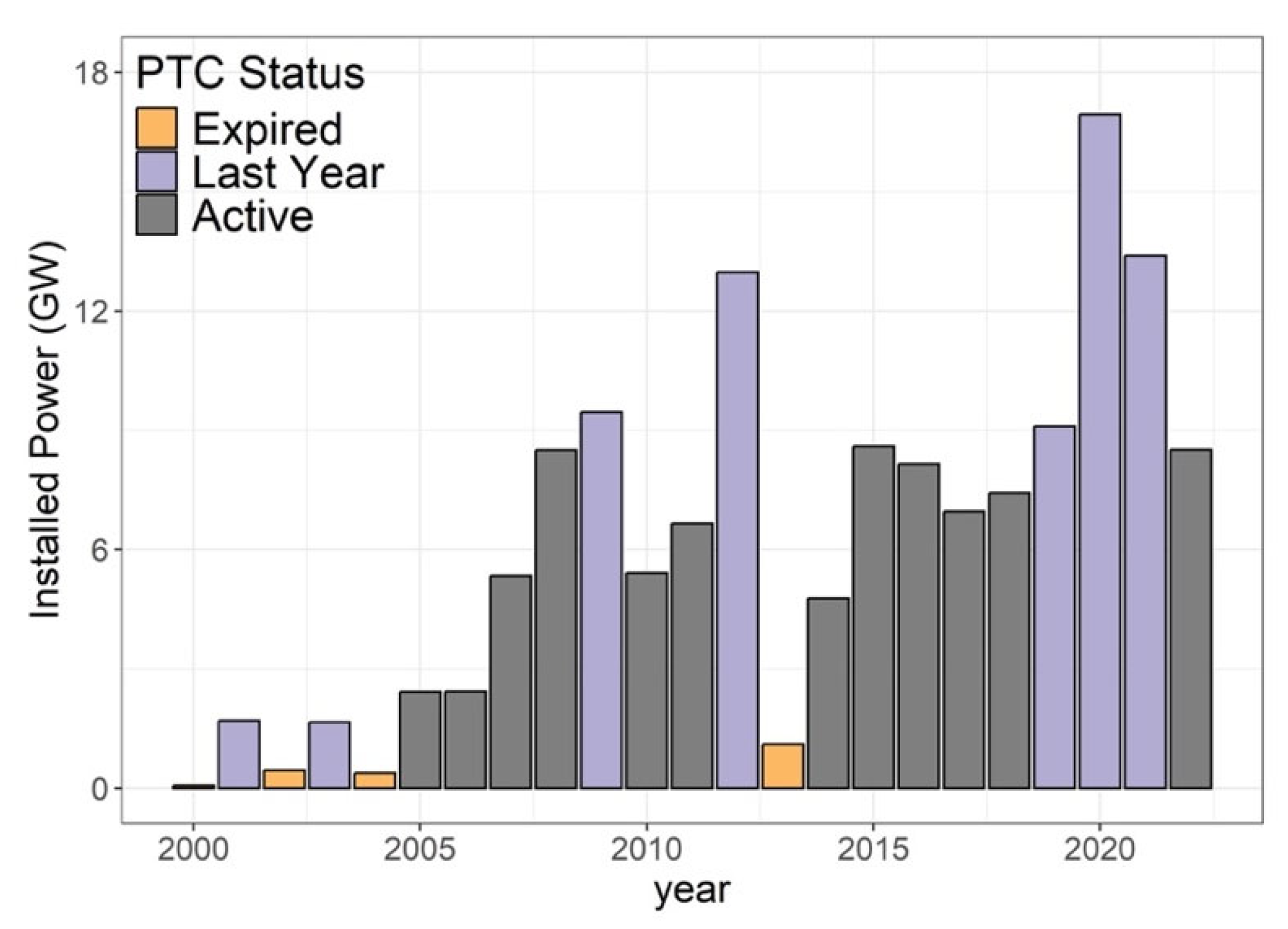
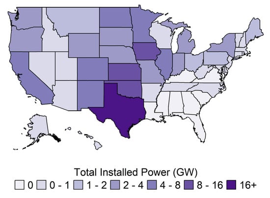
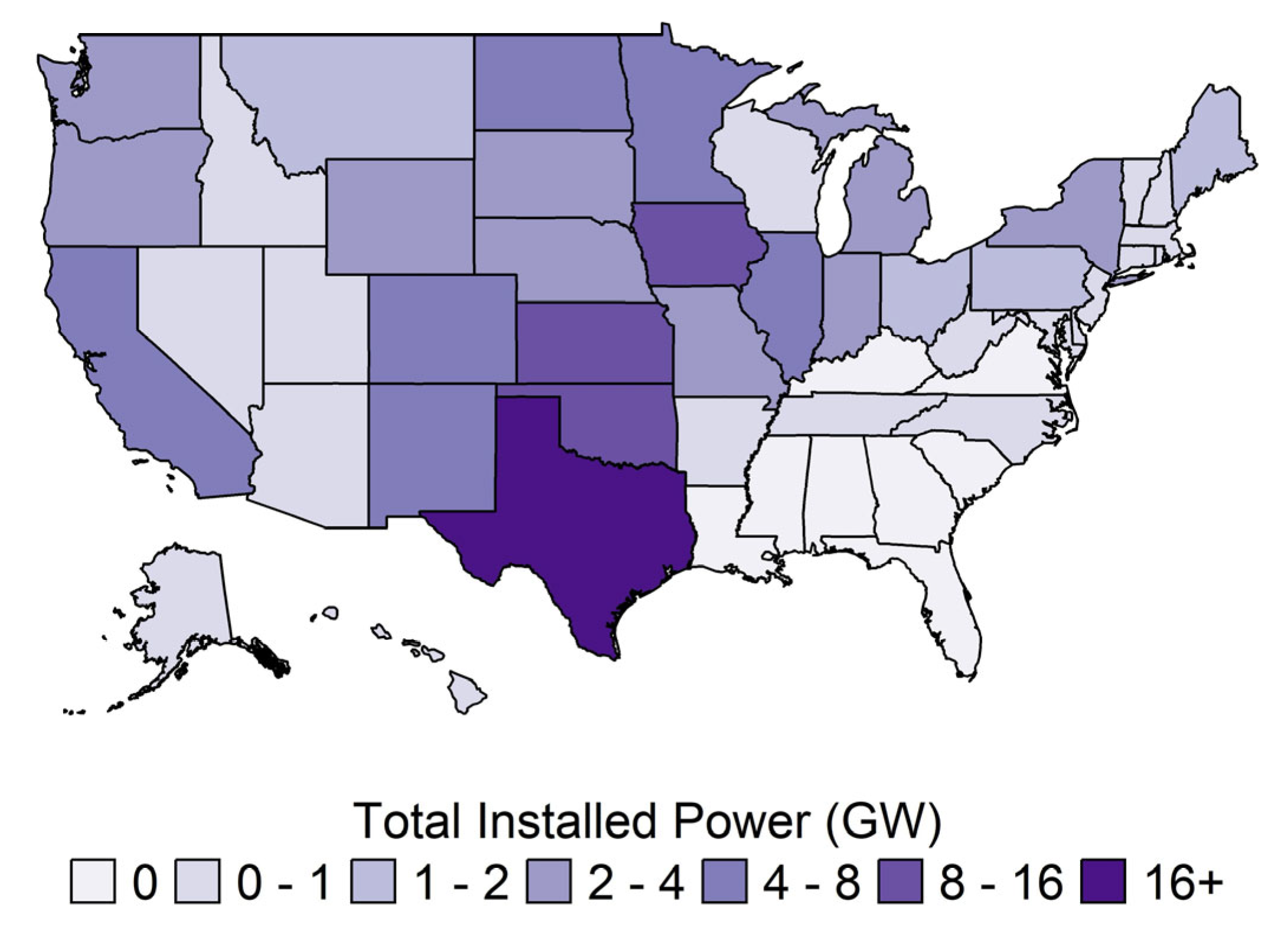
Since the beginning of the 21st century, wind power has developed rapidly, with about 1174 GW of global installed capacity in 2024 [1]. While an order of magnitude smaller than solar, the physical wind resource in the U.S. is large enough to meet all projected electricity demands several times over [2]. Its development has been vigorous, but erratic over both time (in years) and space (among states). Over the 21st century, annual U.S. wind power installations have varied from 0.07 GW installed in 2000, increasing unevenly to a record 14.2 GW in 2020 (Figure 1), then falling to only 5.1 GW in 2024. In the United States, by the end of 2023, 148 GW were installed, providing 425,235 GWh of renewable electricity in that year with very low carbon and water footprints. Briefly in 2024, wind produced more electricity than coal [3] and is poised to exceed coal going forward. Since 2010, installations of wind power have been second only to natural gas, and it was the leading source installed in 2015, 2020, 2021, and 2022 (Table A1). Since 2021, however, solar has led in new electricity generation capacity. In 2025, only 12 percent (7.7 GW) of planned U.S. electrical power additions were wind, well down from a peak of 46 percent of planned capacity additions in 2019 and far behind 52 percent (32.5 GW) of planned capacity in 2025 coming as solar power [4]. Among states, in 2022, Texas led in total capacity at 40.5 GW, 28 percent of a national total of 142.4 GW, while several southeastern states lacked wind power capacity altogether (Figure 2).
Figure 1.
Bar chart of total wind power installations in the U.S. by year 2000–2022, with color indicating years where the Production Tax Credit expired or was set to expire in the following year.
Figure 2.
Installed wind power capacity by state 2000–2022.
The dependent variable this paper seeks to explain is wind power development across space and through time, using data obtained from the U.S. Department of Energy [5]. In 57 percent of 21st century state-years, no wind power was installed at all, while the maximum is 4.3 GW, achieved in Texas in 2019. The coefficient of variation, defined as the standard deviation divided by the mean and providing a measure of relative variability, is over three, reflecting high spatio-temporal variability. Identifying the factors that influence this high variation is therefore of value in evaluating current policies, guiding future policy development, and better understanding wind power development as a process.
In addition to physical wind power capacity as the resource base, several policy factors can potentially affect the development of wind power. Polzin et al. found that policies to promote renewable energy development are most effective when they are designed to reduce financial risk and increase return on investment [6]. For this reason, the Production Tax Credit is a critical US policy [7], yet it has come into and out of effect several times since 2000. The price of wind power development compared to competing electricity sources, especially natural gas and more recently solar, also varies over time across the U.S. Conversely, critical policies such as Renewable Portfolio Standards (RPS) [8], electrical restructuring [9,10], and processes for obtaining site permits [11], vary primarily spatially—among states—while there is also a time signature when they become effective in each state. By examining both spatial and temporal variations, we can better explain wind power development as well as provide a test of the effectiveness of policies implemented to foster it.
Each of these possible drivers of the highly variable phenomenon of wind power development generates questions that can be explored through statistical modeling of empirical data on the installation of wind power in each year or in each state. In the temporal dimension, the research questions ask if wind power development is higher in years when: (a) the Production Tax Credit is in effect, and especially (b) when it is anticipated that it will soon expire, and (c) natural gas prices are high relative to wind power development costs. Wind power development also (d) increases over time reflecting technological improvements in wind turbine design, construction, and management that have occurred at a higher rate than for other energy technologies, except recently for solar photovoltaics. In particular, wind turbines have increased substantially in size over the study period, from about 50 to 130 m rotor diameter and from 60 to 100 m hub height, enabling an increase from about 1 to 3 MW capacity [12].
In the spatial dimension, the research questions are: is wind power development higher in states (e) that have a large total physical wind capacity and (f) consume large quantities of electricity? On the policy front, the questions asked are: is wind power development greater in states (g) where Renewable Portfolio Standards are in effect and (h) does this effect increase over time, (i) where electrical restructuring is not in effect, (j) which are integrated in Regional Transmission Organizations (RTOs) and (k) where legal processes for siting wind farms minimize the opportunity for local opposition to prevent development?
This paper utilizes the capacity of wind power installed in each state in each year from 2000 to 2022 as the dependent variable to be explained by both national temporal and spatial variations in geographical, economic, and policy factors among states that are hypothesized to influence wind power development.
2. Background and Literature Review
2.1. Temporally Variable Factors
2.1.1. Production Tax Credit
First enacted in the Energy Policy Act of 1992 and extended by the Inflation Reduction Act in 2022, the Production Tax Credit (PTC) applies to a variety of renewable energy sources (solar, wind, biomass, geothermal, landfill gas, hydropower, marine hydrokinetic, hydrogen, and nuclear). Wind power construction receives a subsidy of up to $25/MWh for the first 10 years of operation. It was last authorized to apply to wind power projects starting in 2016 with a phase down through 2021 to expire at the end of 2021 [13]. December 2020, immediately before a substantial phase-down, saw the largest surge in wind power project initiations on record [14]. The PTC has been extended several times—in 1999, 2002, 2004, 2005, 2006, 2008, 2009, 2013, 2015, 2019, 2020—with lapses that were retroactively extended. There was also uncertainty about whether it would be extended by Congress as PTC eligibility windows were approached. This policy uncertainty increases risk for investors [6].
Through 2020, the PTC subsidized wind power development by about $30 billion in foregone tax revenues from several thousand claims [15]. In line with multiple studies [2,7,16] we hypothesize that the PTC increases wind power development when it is in effect, and especially in years when it was due to expire, pending subsequent Congressional action. In 2022, Congress passed the Inflation Reduction Act as a tax-credit-based strategy for fostering renewable energy development that was influenced by experience with the PTC, while modifying and extending it. While the Inflation Reduction Act did not come into effect during the study period referenced in this paper, the impact of the Act can be hypothesized to be similar to the PTC.
2.1.2. Relative Cost of Wind Power Development vs. Natural Gas
Since 2014, nearly all new additions to electrical power capacity in the U.S. have been derived from an evolving combination of wind, solar and natural gas, with investment in storage capacity becoming important since 2020 [17] (Table A1). Oil, coal and nuclear power have received little investment; wind power investment, therefore, occurs largely in competition with natural gas and solar power. Given this, high natural gas prices and solar installation costs may favor wind power development, and low prices inhibit it. Borenstein and Bushnell assert that natural gas prices set marginal costs in most electricity systems; this is especially the case in states adopting restructuring [10] (see below). We therefore included data on natural gas prices from EIA [18].
2.2. Spatially Variable Factors
2.2.1. Physical Wind Resources
We hypothesize that the larger the physical potential and density of wind energy potential in a state, the more wind power is developed. The U.S. National Renewable Energy Lab (NREL) estimates the physical resource potential for onshore wind power at 11,000 GW, only seven percent of solar energy potential but over 100 times greater than the technical potential for hydroelectric, biomass or geothermal power [19]. Through 2022, 148 GW had been developed, 1.3 percent of the physical resource potential. Among conterminous U.S. states, this potential at 80 m height varies from 0.2 GW in Rhode Island to 1300 GW in Texas, with the density of physical wind resources varying from 0.002 MW/km2 in Florida, characteristic of the low wind energy potential in the southeast, to 2.388 MW/km2 in Kansas, characteristic of the high wind energy potential in the Great Plains region. The power-generating potential of wind is proportional to the cube of wind speed, thus translating small geographical differences in wind speed into very large differences in wind power potential [20]. This variability also results in low capacity factors (electricity output as a percentage of maximum potential output) for wind power, commonly 25–40 percent [16]. These measures are taken as time invariant; we assume that the annual physical resources available for wind in each state remain constant over the study period.
To date, physical potential exceeds developed resources by a factor of 77 nationally at the end of 2022. This implies that wind power is in an early phase of development, where only the best opportunities among many possible options are being selected for projects. For any natural resource, an efficient process identifies the best quality resources and develops them before accessing lower-quality resources [21]. With respect to energy sources, energy return on energy invested (EROEI) is a widely accepted measuring stick to compare resource quality [22] with a minimum EROEI required to maintain an electrified society [23].
Fossil fuels have been witnessing a steady decline in EROEI [24] as the most easily accessed, highest quality resources are consumed, leaving for future development only poorer quality resources with lower EROEI. Among renewable sources of electricity, hydropower has a very high EROEI [24], but optimal sites are rapidly developed. As increasingly inferior sites are developed, EROEI drops rapidly. In contrast, solar photovoltaics achieve a moderately high EROEI, but with little if any decline as the resource is selectively developed because the density of incoming solar radiation has a small variance geographically. Wind is similar to solar photovoltaics; however, not only does wind speed vary over space more than solar radiation, the cube law cited above exaggerates the differences in wind power potential. Therefore, the EROEI among potential wind power development sites declines faster as the best sites are developed than for solar but not nearly as fast as for hydropower. This means there are far more sites that meet technical criteria for potential wind power development than can be actually developed in a decision-making timeframe. Because the process for selecting sites for wind power development is only partially physically constrained, non-physical economic and policy-related factors, which we identify below, control the selection process.
2.2.2. Electricity Consumption
While many remote areas possess large physical wind resources, electricity produced via wind (or any other source) requires an instantaneous market that is connected to the power source through transmission lines. Wind power produced in one state can be sold in another (especially within regional transmission organizations as discussed below); however, there is no readily available data on how much electricity crosses state lines. Data obtained from the U.S. Energy Information Administration (EIA) on electricity consumed in each state in each year is used as a measure of electricity demand, with the hypothesis that wind power development is positively associated with electricity demand in that state in that year [25].
2.2.3. Electrical Restructuring
Electrical restructuring, as it is usually referred to, is not a policy directed at renewable or wind energy per se. Yet, it has a pervasive effect on electric utilities as institutions and varies among states. It has also had very mixed results as a policy experiment. Prior to the restructuring wave among some states in the 1990s, electric utilities were vertically integrated regulated monopolies that produced power, transported it along transmission lines, and delivered it to customers within a designated service area [10]. Restructuring was borne of the idea that it is only electricity distribution, not production, that is a natural monopoly and that, therefore, electricity production can compete in an open market.
Several states, especially in the northeast, plus Illinois, California, and a few others, forced utilities to divest their power production assets in order to break the vertical integration and concentrate utility efforts on the distribution of electricity. Yet Borenstein and Bushnell characterize the effort as badly mistimed due to the shifting balance between average costs of electricity, which guide regulated prices, and marginal costs, which guide post-restructuring prices in open markets [10]. Utilities sold off power plants at market lows, only to see their value quickly recover as natural gas prices rose. States that did not restructure in the 1990s saw reason to refrain, while some that did so suspended their effort. More recently, however, hydraulic fracturing has resulted in falling natural gas prices [26] making it more competitive relative to wind power.
Borenstein and Bushnell also find that when evaluating the effects of restructuring, there is no difference between treating it as a categorical variable (restructured, not-restructured, suspended) or a continuous variable, such as percent of power produced by independent power producers [10]. We have therefore adopted the former simpler strategy with the hypothesis that restructuring is associated with lower wind power production in line with results from [11]. Of all electricity sources, wind is perhaps the most dependent on vertical integration between building wind power plants (or wind farms) and the transmission capacity to deliver it to market. The higher the proportion of electricity on the grid that is derived from wind power, the more its intermittent nature must be offset by storage, by flexible sources (with natural gas often filling that role), or by electricity demand management [10]. Therefore, there is a measurable cost to wind power’s intermittency, often adding less than 10 percent to cost, but increasing with higher levels of penetration [16]. Recently, electricity storage has been added to vertically integrated projects. Because wind is the power source that is most intermittent and variable, even compared to somewhat more predictable solar, wind benefits most from vertical integration of power production, transmission, and storage—precisely what restructuring undermines.
2.2.4. Regional Transmission Organizations (RTOs)
Initiated in 1999 by the Federal Energy Regulatory Commission (FERC), RTOs organize electricity transmission through regional grids. Over the study period there were seven serving 32 states: California (CA), ERCOT (TX), Midwest (AR, IL, IN, IA, LA, MI, MN, MS, MO, SD, WI), New England (CN, MA, ME, NH, RI, VT), New York (NY), PJM (DE, KY, MD, NJ, OH, PA, VA, WV), and Southwest (KS, NE, OK, SD). While wind power production is intermittent and highly variable, the larger the geographic area in which it is integrated, the lower the variability in capacity factors and power production [27]. For example, Handschy et al. find that low-power hours decline exponentially with the number of wind power sites whose output is aggregated [28]. Therefore, we hypothesize that a state’s presence in an RTO is associated with higher wind power production.
2.2.5. Renewable Portfolio Standards
First enacted in 1983 in Iowa, though not in another state until 1997, Renewable Portfolio Standards (RPS) require that a specific percentage of energy demand be met by designated renewable sources by a specified date. RPS policies are implemented through a system of marketable renewable energy credits [29]. Through 2020, 38 states had enacted RPS [30].
We include RPS as a categorical variable and also as a continuous variable with the number of years it has been in effect as of 2022. The hypothesis states that RPS are associated with higher wind power development over time. Menz and Vachon [31] and Carley [32] found that states with RPS have greater wind power generation than states without, while Yin and Powers [33] show that this effect is influenced by the ambitiousness of the renewable electricity goal. Upton and Snyder, however, refute these results, while also finding that RPS increases electricity prices, and thereby reduces consumption, for meager reductions in greenhouse gas emissions [29]. These reductions are thus attributable not to development of renewables but to reduced electricity consumption in response to price. They thus characterize RPS as a tax that yields no government revenues.
2.2.6. Permitting Processes and Social Acceptance
Much has been written about the social acceptability of wind power, and it clearly affects wind power development—as well as attitudes towards it both before and after deployment. A review by Rand and Hoen of over 130 studies of social acceptability of wind power in North America identifies several themes [34]. North Americans consistently support wind power, but concerns are tied to socioeconomic structures and issues of both procedural and substantive justice, not the so-called “NIMBY” (not in my backyard) effect. Local aesthetic issues, especially visual compatibility with the landscape (which tends to be high in agricultural landscapes), are of greater concern than broad environmental issues such as climate change. Yet it is the exception where developers employ these insights rather than simply try to overcome local opposition when and where it occurs.
One policy variable that we draw from these issues is the wind power plant permitting process that states employ. Research by Bohn and Lant, updated here from the National Conference of State Legislators, shows that several states where there is no or very little wind power development have not developed a permitting system at all (AL, DE, HI, KN, MI, NC, RI, VA) [11,35]. Texas employs a minimal system; Oregon and Washington employ a simplified system at the state level. The remaining 39 states employ a standard system that facilitates local input and requires local approval. While we favor the standard system because it facilitates local input in a democratic process, we hypothesize that it is associated with lower wind power development because it empowers local concerns and potentially causes delays or rejections of proposals in a manner that is undesirable from the perspective of developers.
3. Statistical Methods and Results
Ideally, the statistical analysis would proceed with full consideration of each state over time. However, this is not feasible given the inherent limits on population size (50 states, 23 years) and the frequency distribution of the data, where the majority of state-year combinations have no wind power development. Several southeastern states record no wind power development over the study period, making it impossible to determine what variables, if any, would affect wind power development in those states. Other states only have a few years of wind power development, which again makes it difficult to quantify the effects of any one variable. Lastly, many state-level policies, along with the physical features of the state such as size and wind power potential, remain constant over the study period. This means that state-time models would fail to capture the effect of the variables of greatest interest in our study since those variables tend to remain mostly constant over time.
Our analysis proceeds in two steps to make the most efficient use of our small population size. The first set of models look at aggregate wind power generation nationally over time. These models allow us to see how total national wind power development responds to federal policy and prices, without considering the state-level effects. The second set of models looks at aggregate wind power across time within each state. These models show us what state-level policies and attributes are most predictive in a state’s choice to construct wind power over the study period. We recognize that such an approach limits our ability to explore the response of wind power construction to annual scale changes in electricity prices or demand. The often-lengthy process for wind power permitting and the long-term nature of the investment, however, make it difficult for the industry to respond instantaneously to annual level fluctuations in prices. Also, long-term variations in prices across states can still be effectively captured in the aggregate models. All that in mind, the time-dependent and state-dependent models provide valuable insight into what combination of state and federal level policies is most associated with investment in wind power capacity.
3.1. Data
Publicly available data (Table 1) were organized by state-year and were analyzed and visualized using R 4.4.0 [36] with the help of the dplyr [37], ggplot2 [38], ggrepel [39], and fiftystater [40] R packages.
Table 1.
Sources of data used in this study.
3.2. Temporal Analysis
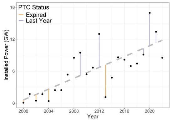
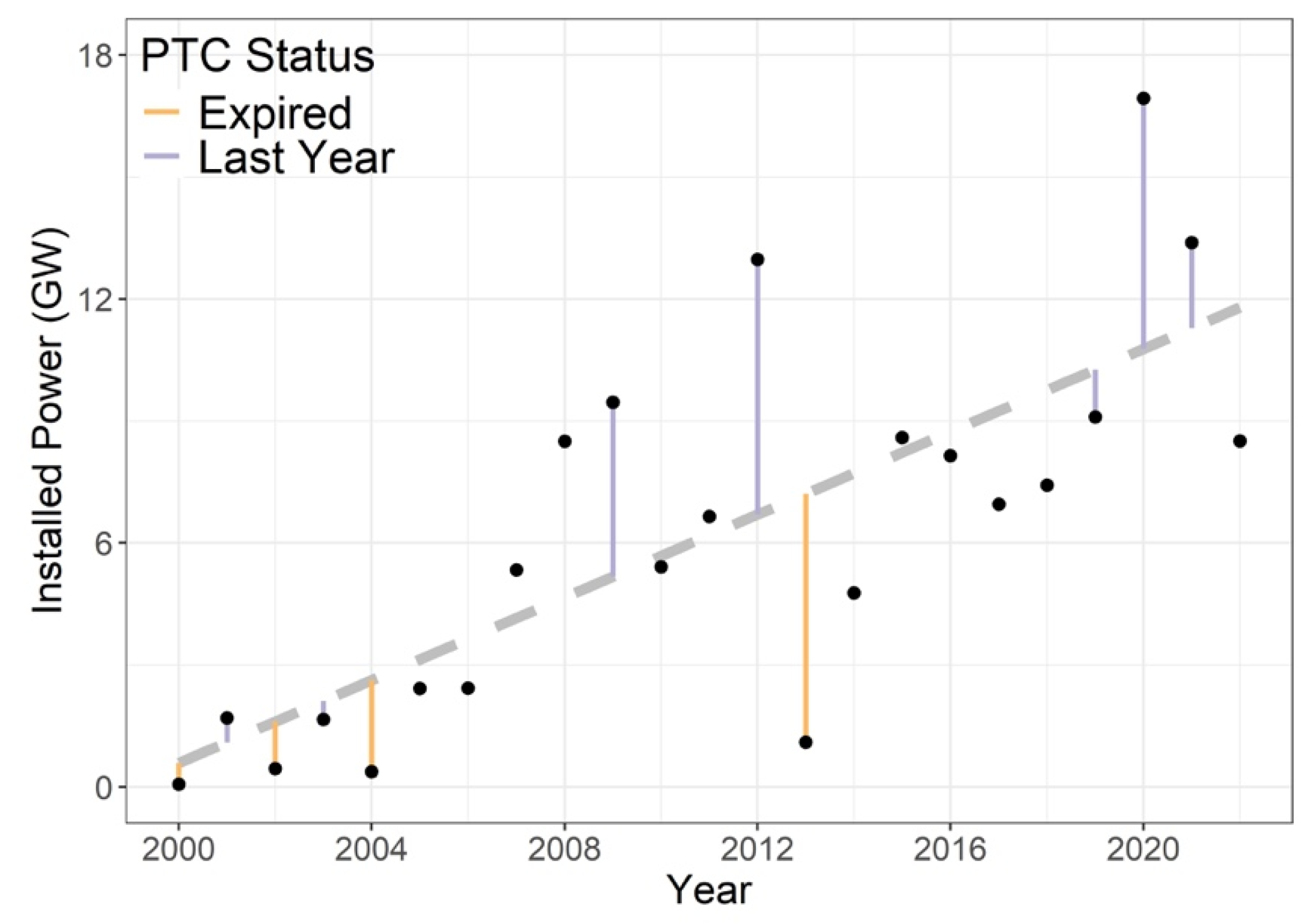
For federal policies that vary temporally, we explore the aggregate wind power constructed nationally in each year. We include a time trend, natural gas prices, whether the PTC was in effect, and the number of years before it was scheduled to expire. Figure 3 shows that wind power development increased roughly linearly over time through the 2000–2022 study period. Interestingly, the largest residuals are all associated with the PTC; less development than expected (in orange) when it expires (2000, 2002, 2004, 2011), and more than expected (in purple) when it is scheduled to expire the following year (2009, 2011, 2020, 2021).
Figure 3.
Linear model relating total installed wind power in the U.S. as a function of time, emphasizing model residuals in years where the Production Tax Credit expired or was set to expire in the following year.
This outcome motivates the creation of a linear model that includes both the effects of time and the PTC. A linear model is used in this case because (1) we observe that the time-dependent trend in wind power is linear, (2) we have a relatively small population of 23 years, and (3) we have a limited number of explanatory variables, since all the state-level variables become irrelevant when aggregating across space. Any attempts to use more complex modeling techniques in this context would have diminishing returns with a limited study period and a limited number of variables.
This model is formulated as:
where y represents total installed wind power capacity (in GW), represents PTC being in effect (and 0 otherwise), represents the PTC in its last guaranteed year (and 0 otherwise), and t represents the number of years since 2000.
Coefficients for this model are:
The coefficients and are clearly related; PTC promotes wind power development by 2.53 GW nationally whenever it is in effect, with an additional rush to develop of 3.17 GW when it is anticipated to expire. A subset F test reveals that the collective inclusion of and is highly significant (p-value of 0.006 < 0.01). We also observe that the full model (including time and PTC variables) satisfies the assumptions of regression, including residuals that are approximately normally distributed with no serious indications of heteroskedasticity (Appendix A, Figure A1).
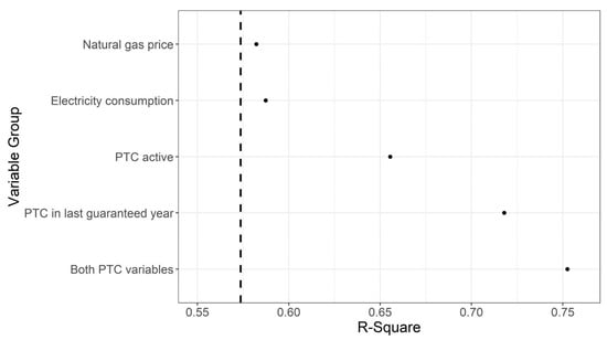
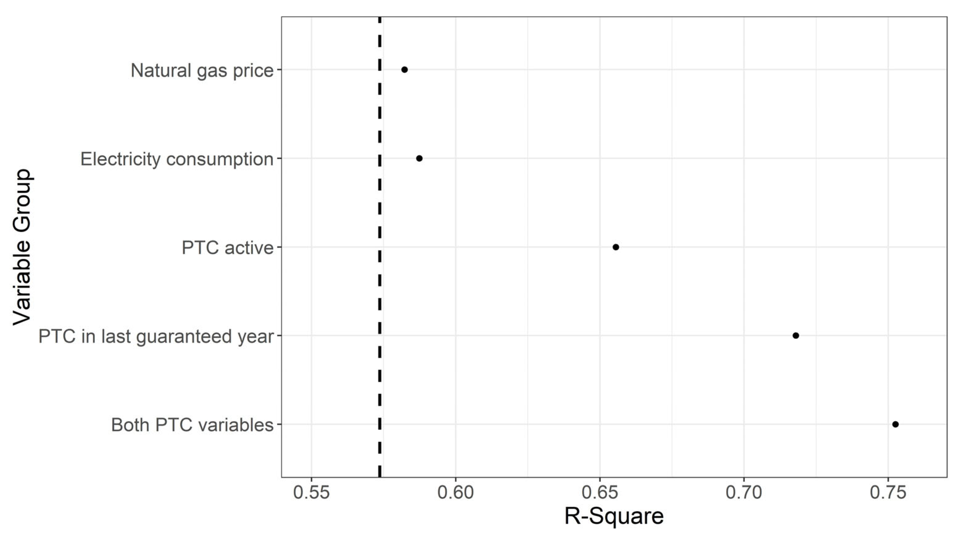
We further tested the extent to which other temporally variant variables are able to improve explanation relative to a model including only the time trend (R2 = 0.57) (Figure 4). Natural gas prices do little to improve the explanatory power of the linear time-trend model, but the two categorical PTC variables and improve the model R2 from 0.57 to 0.76.
Figure 4.
Dot-chart of the multiple linear regression R2 value when each variable is added to a linear regression model that accounts for the effect of time. The dashed line represents the R2 value for the simple linear regression model that only includes time.
3.3. Variance Among States
Unlike the PTC, many state policies are in place or, if a change in state policy is made, it occurs only once. This compels us to consider each state’s cumulative wind power construction over the study period 2000–2022. The distribution of wind power construction by state is highly skewed, but the skewness can be mitigated with a log (x + 1) transformation (Appendix A, Figure A2).
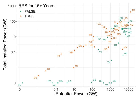
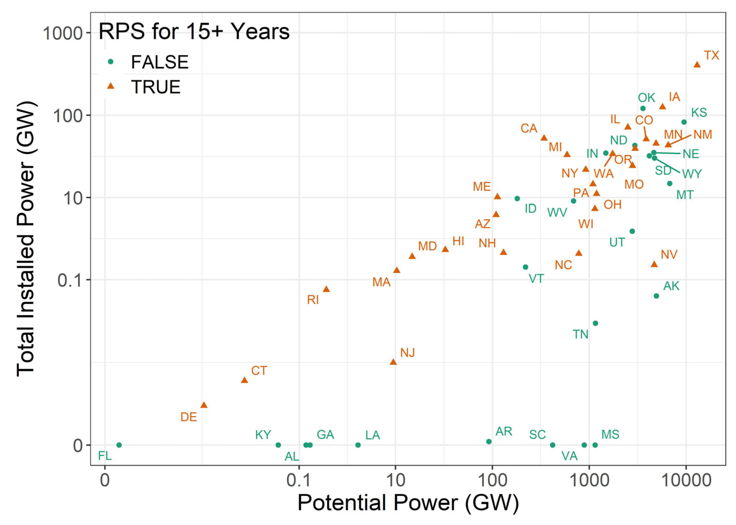
The log-log relationship between total wind power development and wind power potential is strong, but non-linear, with several states where development is absent (Figure 5). The difficulty of satisfying the assumptions of regression, coupled with the large number of categorical variables, motivates the use of a machine learning approach for modeling the expected wind power generation across states. Random forests [44] are selected for their robustness to small sample sizes relative to other machine learning methods. The method also has built-in ways to measure predictive accuracy through the out-of-bag (OOB) error, as well as variable importance.
Figure 5.
Scatterplot of the relationship between wind power potential and total installed wind power by state 2000 to 2022. The presence of Renewable Portfolio Standards for at least 15 years is color-coded.
Random forest is a methodology that creates a set of regression trees using bootstrap samples of the data. This means that each tree in the forest is constructed using roughly 67 percent of the original observations, with some observations being repeated more than once as part of the bootstrap sampling technique. Final predictions for the random forest are simply the average of the predictions of the individual trees in the forest. The method has been popular for more than 20 years, largely due to the small number of hyperparameters relative to other machine learning methods. In this study, we use a random forest model for the following reasons. First, we do not have good parametric (i.e., equation-based) relationships between the explanatory variables and the response variable. Second, we need the ability to model interactions between the explanatory variables and the response variable, which is something difficult to do with parametric models, but natural to do in a random forest. Third, we need a method that allows for exploration of variable importance, which is something built directly into the random forest methodology.
We ran a random forest model using the ranger R package [45] containing state area, wind power potential, mean electric sales, mean natural gas cost, the number of years that renewable portfolio standards (RPS) have been in place, the presence or absence of a regional transmission organization (RTO) and electrical restructuring, and the predominant system for permitting projects. Because more trees have been shown to provide more robust measures of permutation variable importance [46], our random forest model includes 2000 trees. All other random forest hyperparameters are left fixed at the default function values, as Random Forest models are known to be relatively robust to changes in the hyperparameters, and there is no need to fully optimize predictive accuracy for an exploratory model. The model measures the permutation variable importance, which is defined as the loss in predictive accuracy resulting from the randomization of the values of a variable. Permutation variable importance thus measures how often a variable is used in the random forest model predictions. This is different than the loss in accuracy resulting from removing a variable entirely from a study. Indeed, Schumaker et al. illustrates that a variable can have a high permutation variable importance measure, yet still not be required for accurate predictions [47]. For this reason, this paper explores both the permutation variable importance as well as the variable omission importance.
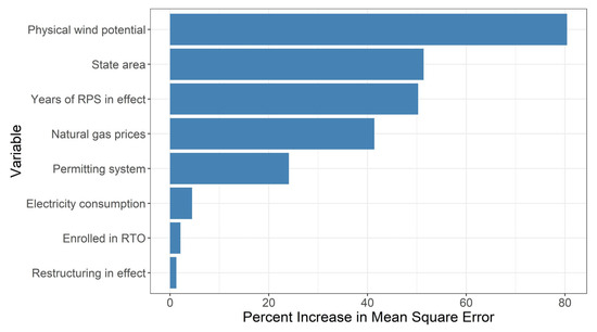
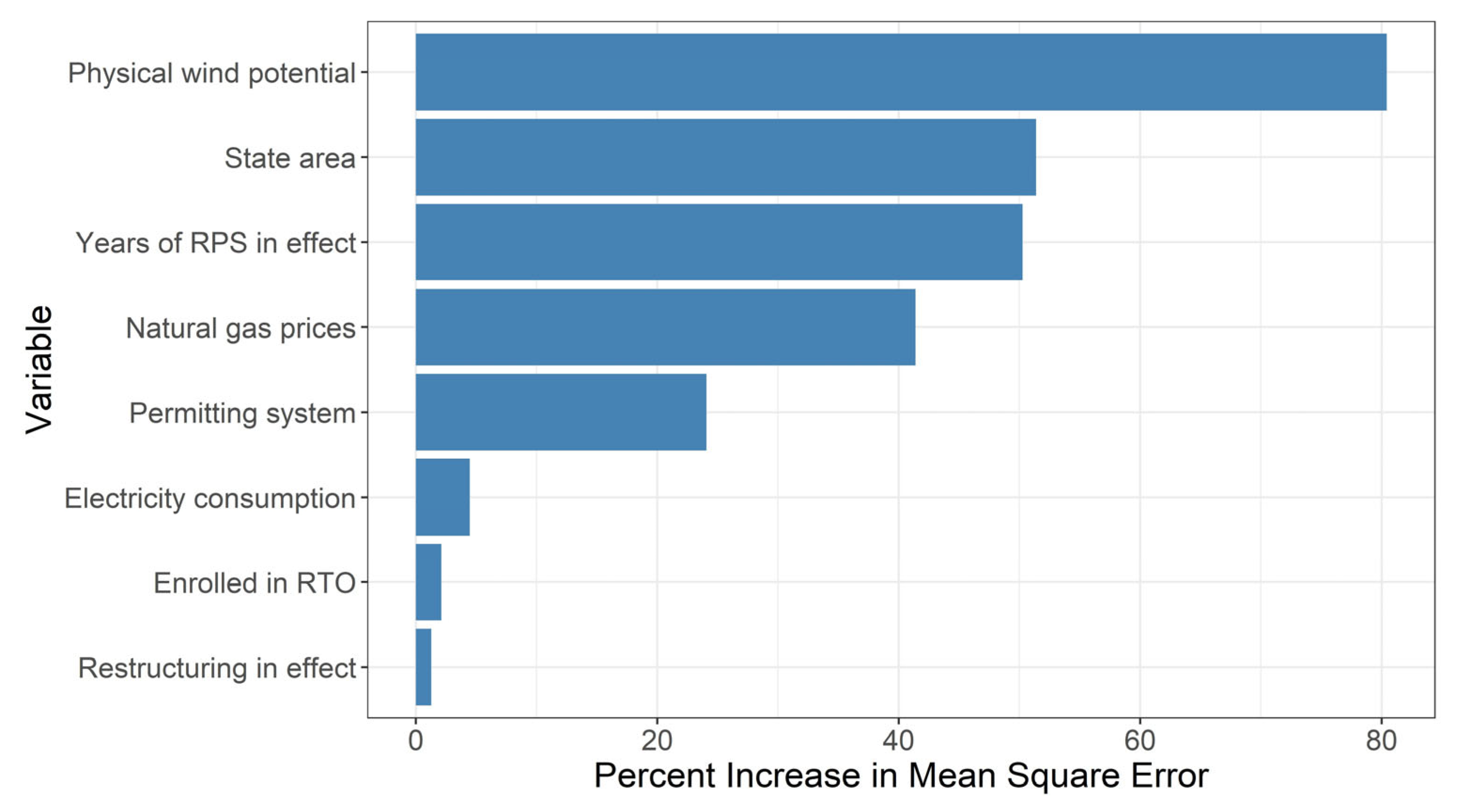
Physical capacity for wind generation and the area of a state, factors that define the geographic suitability of wind power, are the most important predictor of wind power generation among states (Figure 6). Among policy and economic variables, the most important are the presence of renewable portfolio standards, the average cost of natural gas, and the type of permitting system.
Figure 6.
Variable importance plot showing the percentage increase in the Random Forest Out of Bag (OOB) Mean Square Error (MSE) when each variable is randomly permuted. Larger increases in OOB MSE indicate that a variable is more important in prediction.
To explore the variable importance of each candidate explanatory variable, we performed the following:
Step 1: Fit a Random Forest model to the log-transform of the log-transform of aggregate wind power installed, removing one of the variables referenced in Figure 6.
Step 2: Extract the Out of Bag (OOB) R2, which is a measure of the percentage variance explained, for each model.
Step 3: Because OOB R2 depends on the random sub-setting of the observations in each of the trees in the forest, we repeated Steps 1 and 2 100 times for each Random Forest model while keeping track of the range of OOB R2 values for each model.
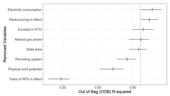
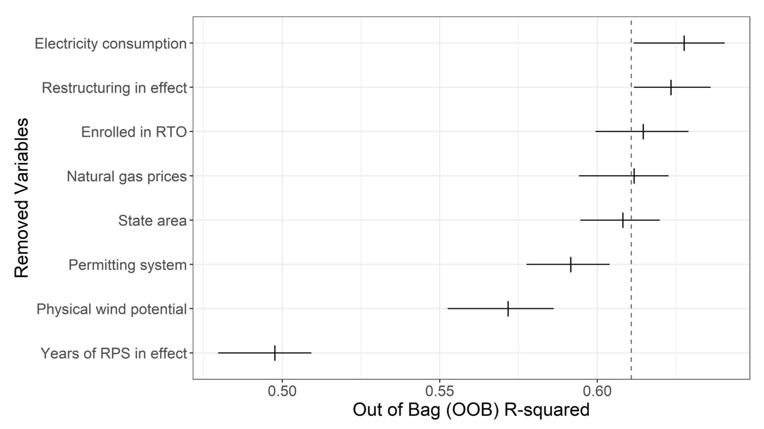
Figure 7 shows the range of OOB R2 (with medians denoted by tick marks), and the y-axis shows the variable that was removed for the calculation of the OOB R2. The length of the line segments in Figure 7 provides a measure of the sensitivity of the accuracy results to the randomness inherent in the Random Forest model. Lines with lower OOB R2 are evidence of higher variable importance because the loss in explanatory power of the model is greater.
Figure 7.
Plot comparing the change in the OOB R2 value when each variable is removed from the model (dashed line is model R2). Larger reductions in the OOB R2 mean that the model was unable to compensate for the loss of that variable when it was removed from the equation.
Note that the exclusion of electricity sales, electricity restructuring, and regional transmission organization leads to a slight increase in the OOB R2, showing that these variables do not help explain wind power development among states. Instead, wind power generation potential and, especially, renewable portfolio standards have the most predictive power, while permitting systems and natural gas prices have marginal predictive power. This variable omission importance also highlights the potential for correlation among the explanatory variables. For example, wind potential is highly correlated with state area, meaning that a model that omits one of those variables can at least partially compensate in prediction by using the other variable. By leaving both wind potential and state area in the model at the same time, we can quantify how much better a predictor wind potential is compared to state area, as best observed in Figure 7. In this figure, we observe that the removal of state area results in no loss in the percent variance explained compared to the baseline Random Forest model, but the removal of wind power potential results in a four percent reduction in the percent variance explained. This quantifies the usefulness of wind potential as an included variable as opposed to using the easier-to-obtain state area variable in prediction. When moving from exploratory analysis to predictive analysis, we would recommend that only wind power potential be used in predictive models, with the state area variable being omitted.
Taken together, Figure 6 and Figure 7 highlight that, as expected, wind power potential is the most important variable for predicting state-level wind power construction. Additionally, the existence of renewable portfolio standards is the most indispensable explanatory variable, as its effect cannot be explained by any other combination of explanatory variables. Lastly, the effect of all other explanatory variables is marginal to non-existent. The identification of the unimportant variables is at least as interesting as the identification of the important variables, as it suggests that aggregate economic data related to electricity demand and pricing, as well as aggregated information related to electric grid organization and restructuring, are not meaningful predictors of wind power construction.
The results from Figure 6 and Figure 7 motivate a two-state hurdle model of total wind power generation while accounting for the excess zero values. Let megawatt denote the threshold for the stage one model. The use of 1 MW as a threshold accommodates the negligible amount of wind power constructed in the state of Arkansas. Assume that when exceeds the threshold and zero otherwise, with representing the probability that . The stage one model takes the form
where represents wind power potential and represents the existence of an RPS for at least 15 years. The choice to model RPS as a binary variable in this case is motivated by the oddly shaped distribution of RPS, with most states having either zero or 23 years of RPS, with few observations scattered in between. This was not a concern in the Random Forest model due to the non-parametric nature of that method, but it is something that must be considered in this parametric model alternative.
The stage two model takes the form
where all values of exceeding 1 MW are assumed to follow a gamma distribution with mean . We note that we also considered the potential of an interaction term (e.g., ), but the term proved to be highly non-significant and was thus removed in order to focus on the additive effects.
The nature of the data, as previously observed in Figure 5, makes it impossible to numerically fit the stage one model since none of the states with near-zero wind power installations have an RPS. Thus, the presence of an RPS for at least 15 years is a perfect predictor of the existence of some wind-power installation over the study period. For the stage two model, the results are given as
This model shows that the effect of wind power potential and RPS are both positive, but that the effect of log wind potential is highly significant (p-value < 0.001), while the effect of RPS is marginally non-significant (p-value = 0.08). Given the results from Figure 6 and Figure 7, this model suggests that RPS is a useful variable in identifying which states choose to build no wind power capacity over the study period, but is not a useful variable in predicting wind power generation among the subset of states with a non-trivial amount of wind-power construction.
We note that all of these methods are an exploration in predictive power. In a purely observational study with small population sizes, we are unable to determine what effects are causal. That said, understanding the strength of associations is a useful step in determining the potential impact, or lack of impact, that these policies and attributes have on wind power generation. Additionally, understanding which variables are not associated with wind power generation is equally important, as a lack of an association implies a lack of causality. This is especially important when considering insensitivity of wind power generation to state-level differences in electricity prices and demand, the existence of a rational transmission organization, electrical restructuring, or wind farm permitting systems.
4. Conclusions and Policy Implications
Statistical results provide a clear picture of factors that promote wind power development in the U.S. It occurs when federal tax credits are available, and even more so when they are anticipated to expire. It occurs in states with high physical wind potential. These states tend to pass Renewable Portfolio Standards but RPS have no measurable effect on the capacity of wind power installed. Permitting systems that deflect local opposition and natural gas prices have a statistically marginal effect, while electrical restructuring, enrollment in a regional transmission organization, and other factors do not have a measurable effect.
These results indicate that PTC-like tax credits offered through the Inflation Reduction Act are critical in fostering continued wind power development. With Inflation Reduction Act tax credits expiring at the end of 2025, wind power capacity grew by an estimated 7 Gigawatts in 2025 [48] compared to 5.1 Gigawatts in 2024, despite direct intervention to retard wind power development by the Trump Administration and the growing cost advantage of solar, which enjoys similar tax credits, over wind power. This surge serves as a form of validation of the model presented.
While the year-before-expiration effect is clear, there is no way to experimentally or statistically determine whether turning credits on and off results in greater development than a more consistent policy. Moreover, the shifting availability of tax credits results from political struggles in Congress rather than an attempt to manage wind power development. Barradale found that, in the context of power purchasing agreement negotiations, policy uncertainty drives investment volatility [7]. Shafiullah et al., and Shang et al. similarly find that economic policy uncertainty reduces investment in renewable energy in the US, while Sun et al. find this effect globally [49,50,51]. We therefore do not recommend, for example, turning the Inflation Reduction Act on and off, as it is unclear whether the surge in development in pre-expiration years offsets the suppression of development in post-expiration years.
Results also indicate that renewable portfolio standards are a strong separator of states that choose to engage in wind power construction and those that do not. However, in states with consistent wind power generation, the influence of renewable portfolio standards on wind power generation is marginal and not statistically significant. This is consistent with Upton and Snyder, who point out that RPS are inefficient compared with direct economic incentives like production tax credits [29].
Supplementary Materials
The following supporting information can be downloaded at: https://www.mdpi.com/article/10.3390/en19020520/s1.
Author Contributions
Conceptualization C.L.L.; Data curation E.R. and C.L.L.; Formal analysis E.R., M.M.A., B.B., R.S., and C.L.L.; Funding acquisition E.R.; Investigation E.R., C.L.L., and M.M.A.; Methodology B.B. and R.S.; Project administration C.L.L.; Resources C.L.L.; Software B.B.; Supervision C.L.L.; Validation B.B.; Visualization M.M.A. and B.B.; Roles/Writing—original draft C.L.L. and B.B.; Writing—review & Editing M.M.A., B.B., R.S. and C.L.L. All authors have read and agreed to the published version of the manuscript.
Funding
Utah State University Undergraduate Research and Creative Opportunities grant.
Data Availability Statement
The original contributions presented in this study are included in the article and Supplementary Material. Further inquiries can be directed to the corresponding author.
Conflicts of Interest
The authors declare no conflicts of interest.
Abbreviations
The following abbreviations are used in this manuscript:
| RPS | Renewable Portfolio Standards |
| RTOs | Regional Transmission Organizations |
| PTC | Production Tax Credit |
| NREL | National Renewable Energy Lab |
| EROEI | energy return on energy invested |
| EIA | Energy Information Administration |
| FERC | Federal Energy Regulatory Commission |
| NIMBY | not in my backyard |
Appendix A
Figure A1.
Plots showing the normality and the constant variance of the residuals from the linear model containing the time and PTC variables. The blue line in the right plot shows the moving average of the residuals, while the gray band shows the confidence interval. This shows that the residuals do not substantially deviate from zero, relative to the natural variance, over the range of the predicted values.
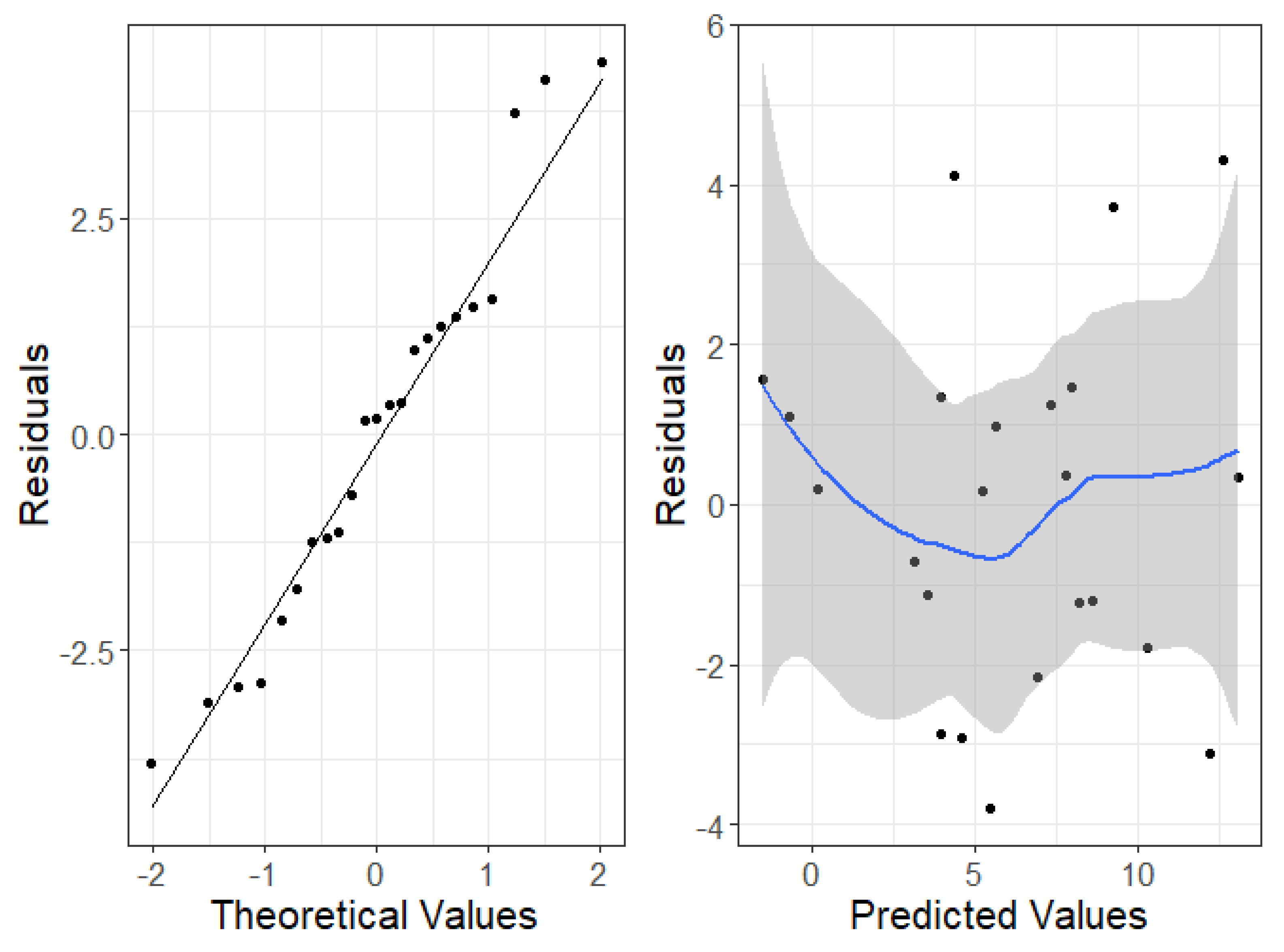
Figure A2.
Histograms of total wind power construction by state on traditional and log scales.
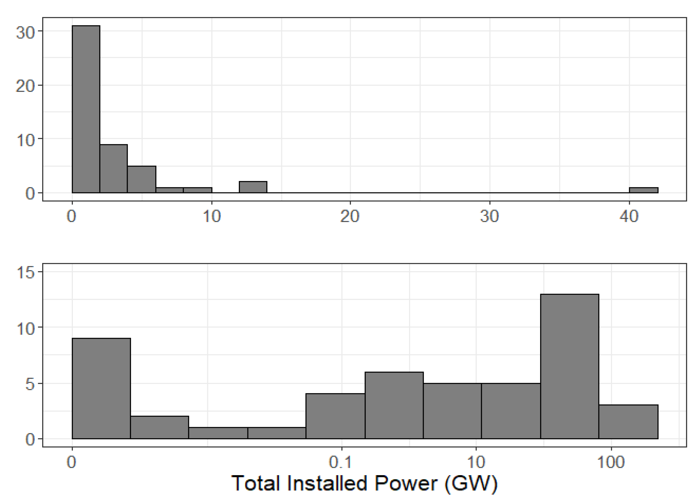
Table A1.
Percent U.S. Electric Utility-Scale Capacity Additions by Fuel Type, 2010–2024.
References
- World Wind Energy Association. World Wind Energy Association, Annual Report 2024; World Wind Energy Association: Bonn, Germany, 2025. [Google Scholar]
- Lu, X.; Tchou, J.; McElroy, M.B.; Nielsen, C.L. The Impacts of Production Tax Credits on the profitable production of electricity from wind in the U.S. Energy Policy 2011, 39, 4207–4214. [Google Scholar] [CrossRef] [Scilit]
- US Energy Information Administration. Today in Energy: US Wind Generation Hits Record in April 2024, Exceeding Coal-Fired Generation. 2025. Available online: https://www.eia.gov/todayinenergy/detail.php?id=62784 (accessed on 20 February 2025).
- U.S. Energy Information Administration. Solar, Battery Storage to Lead New US Generating Capacity Additions in 2025. 2025. Available online: https://www.eia.gov/todayinenergy/detail.php?id=64586#:~:text=Together%2C%20solar%20and%20battery%20storage,of%20capacity%20additions%20last%20year (accessed on 1 May 2025).
- U.S. Department of Energy. Land Based Wind Market Reports; Office of Energy Efficiency and Renewable Energy: Washington, DC, USA, 2023.
- Polzin, F.; Egli, F.; Steffen, B.; Schmidt, T.S. How do policies mobilize private finance for renewable energy?—A systematic review with an investor perspective. Appl. Energy 2019, 236, 1249–1268. [Google Scholar] [CrossRef] [Scilit]
- Barradale, M.J. Impact of public policy uncertainty on renewable energy investment: Wind power and the production tax credit. Energy Policy 2010, 38, 7698–7709. [Google Scholar] [CrossRef] [Scilit]
- Carley, S. State renewable energy electricity policies: An empirical evaluation of effectiveness. Energy Policy 2009, 37, 3071–3081. [Google Scholar] [CrossRef] [Scilit]
- Heiman, M.K. Expectations for renewable energy under market restructuring: The U.S. experience. Energy 2006, 31, 1052–1066. [Google Scholar] [CrossRef] [Scilit]
- Borenstein, S.; Bushnell, J. The U.S. electricity industry after 20 years of restructuring. Annu. Rev. Econ. 2015, 7, 437–463. [Google Scholar] [CrossRef] [Scilit]
- Bohn, C.; Lant, C.L. Welcoming the wind? Determinants of wind power development among U.S. states. Prof. Geogr. 2009, 61, 87–100. [Google Scholar] [CrossRef] [Scilit]
- U.S. Department of Energy. Wind Turbines: The Bigger, the Better. 2024. Available online: https://www.energy.gov/cmei/articles/wind-turbines-bigger-better (accessed on 19 December 2025).
- U.S. Environmental Protection Agency. Renewable Electricity Production Tax Credit Information. 2021. Available online: https://www.epa.gov/lmop/renewable-electricity-production-tax-credit-information (accessed on 5 October 2021).
- U.S. Energy Information Administration. 2021. Available online: https://www.eia.gov/energyexplained/electricity/electricity-in-the-us.php (accessed on 30 September 2021).
- Congressional Research Service. The Renewable Electricity Production Tax Credit: In Brief. 2020. Available online: https://sgp.fas.org/crs/misc/R43453.pdf (accessed on 3 October 2025).
- Hitaj, C. Wind power development in the United States. J. Environ. Econ. Manag. 2013, 65, 394–410. [Google Scholar] [CrossRef] [Scilit]
- Solar Energy Industries Association. Solar Market Insight Report 2024 Year in Review. 2025. Available online: https://seia.org/research-resources/solar-market-insight-report-2024-year-in-review/ (accessed on 18 December 2025).
- U.S. Energy Information Agency. Natural Gas Prices. 2024. Available online: https://www3.eia.gov/dnav/ng/ng_pri_sum_dcu_SAL_a.htm (accessed on 21 May 2024).
- National Renewable Energy Lab. Renewable Energy Technical Potential. 2012. Available online: https://www.nrel.gov/gis/re-potential.html (accessed on 13 October 2021).
- International Renewable Energy Agency. Wind Energy. 2025. Available online: https://www.irena.org/Energy-Transition/Technology/Wind-energy (accessed on 19 December 2025).
- Hall, C.A.S.; Cleveland, C.J. Petroleum drilling and production in the United States: Yield per effort and net energy analysis. Science 1981, 211, 576–579. [Google Scholar] [CrossRef] [Scilit]
- Hall, C.A.S.; Klitgaard, K. Energy and the Wealth of Nations: An Introduction to Biophysical Economics, 2nd ed.; Springer: Berlin/Heidelberg, Germany, 2018. [Google Scholar]
- Hall, C.A.S.; Balogh, S.; Murphy, D.J.R. What is the minimum EROI that a sustainable society must have? Energies 2009, 2, 25–47. [Google Scholar] [CrossRef] [Scilit]
- Murphy, D.J.; Raugei, M.; Carbajales-Dale, M.; Rubio Estrada, B. Energy return on investment of major energy carriers: Review and harmonization. Sustainability 2022, 14, 7098. [Google Scholar] [CrossRef] [Scilit]
- U.S. Energy Information Agency. Retail Sales of Electricity to Ultimate Customers. 2024. Available online: https://www.eia.gov/electricity/data.php (accessed on 20 May 2024).
- Feng, G.F.; Wang, Q.J.; Chu, Y.; Wen, J.; Chang, C.P. Does the shale gas boom change the natural gas price-production relationship? Evidence from the US market. Energy Econ. 2021, 93, 104327. [Google Scholar] [CrossRef] [Scilit]
- Fisher, S.; Schoof, J.; Lant, C.; Therrell, M. The effect of geographical distribution on the reliability of wind energy. Appl. Geogr. 2013, 40, 83–89. [Google Scholar] [CrossRef] [Scilit]
- Handschy, M.A.; Rose, S.; Apt, J. Is it always windy somewhere? Occurrence of low-wind-power events over large areas. Renew. Energy 2017, 101, 1124–1130. [Google Scholar] [CrossRef] [Scilit]
- Upton, G.B.; Snyder, B.F. Funding renewable energy: An analysis of renewable portfolio standards. Energy Econ. 2017, 66, 205–216. [Google Scholar] [CrossRef] [Scilit]
- U.S. Energy Information Administration. Renewable Energy Explained: Portfolio Standards. 2021. Available online: https://www.eia.gov/energyexplained/renewable-sources/portfolio-standards.php (accessed on 7 October 2021).
- Menz, F.C.; Vachon, S. The effectiveness of different policy regimes for promoting wind power: Experiences from the states. Energy Policy 2006, 34, 1786–1796. [Google Scholar] [CrossRef] [Scilit]
- Carley, S.; Baldwin, E.; MacLean, L.M.; Brass, J.N. Global expansion of renewable energy generation: An analysis of policy instruments. Environ. Resour. Econ. 2016, 68, 397–440. [Google Scholar] [CrossRef] [Scilit]
- Yin, H.; Powers, N. Do states renewable portfolio standards promote in-state renewable generation? Energy Policy 2010, 38, 1140–1149. [Google Scholar] [CrossRef] [Scilit]
- Rand, J.; Hoen, B. Thirty years of North American wind energy acceptance research: What have we learned? Energy Res. Soc. Sci. 2017, 29, 135–148. [Google Scholar] [CrossRef] [Scilit]
- National Conference of State Legislatures. State Approaches to Wind Facility Siting. 2024. Available online: https://www.ncsl.org/energy/state-approaches-to-wind-facility-siting#:~:text=In%20at%20least%2022%20states%2C%20siting%20regulations%20are,with%20only%20state-level%20rules%20for%20decommissioning%20wind%20projects (accessed on 21 May 2024).
- R Core Team. _R: A Language and Environment for Statistical Computing_, R Foundation for Statistical Computing: Vienna, Austria, 2024. Available online: https://www.R-project.org/ (accessed on 12 October 2025).
- Wickham, H.; François, R.; Henry, L.; Müller, K.; Vaughan, D. _dplyr: A Grammar of Data Manipulation_. R Package Version 1.1.4. 2023. Available online: https://CRAN.R-project.org/package=dplyr (accessed on 12 October 2025).
- Wickham, H. ggplot2: Elegant Graphics for Data Analysis; Springer: New York, NY, USA, 2016. [Google Scholar]
- Slowikowski, K. _ggrepel: Automatically Position Non-Overlapping Text Labels with ‘ggplot2’_. R Package Version 0.9.6. 2024. Available online: https://CRAN.R-project.org/package=ggrepel (accessed on 12 October 2025).
- Murphy, W. Fiftystater: Map Data to Visualize the Fifty U.S. States with Alaska and Hawaii Insets_. R Package Version 1.0.1. 2025. Available online: https://github.com/wmurphyrd/fiftystater (accessed on 12 October 2025).
- National Conference of State Legislatures. State Renewable Portfolio Standards and Goals. 2021. Available online: https://www.ncsl.org/energy/state-renewable-portfolio-standards-and-goals (accessed on 20 May 2024).
- Sonenshine, R. Effect of Utility Deregulation and Mergers on Consumer Welfare; Universe Scientific Publishing: Singapore, 2017; Volume 2, pp. 1–13. [Google Scholar]
- Federal Energy Regulation Commission (FERC). Order No. 2000—Regional Transmission Organizations; Federal Energy Regulatory Commission: Washington, DC, USA, 1999.
- Breiman, L. Random forests. Mach. Learn. 2001, 45, 5–32. [Google Scholar] [CrossRef] [Scilit]
- Wright, M.N.; Ziegler, A. ranger: A Fast Implementation of Random Forests for High Dimensional Data in C++ and R. J. Stat. Softw. 2017, 77, 1–17. [Google Scholar] [CrossRef] [Scilit]
- Probst, P.; Wright, M.N.; Boulesteix, A.L. Hyperparameters and tuning strategies for random forest. WIREs Data Min. Knowl. Discov. 2019, 9, e1301. [Google Scholar] [CrossRef] [Scilit]
- Schumaker, B.L.; Burchfield, E.K.; Bean, B.; Yost, M.A. Leveraging important covariate groups for corn yield prediction. Agriculture 2023, 13, 618. [Google Scholar] [CrossRef] [Scilit]
- Wood-Mackensie. US Wind Energy Monitor, Q4 2025; Wood-Mackensie: Edinburgh, UK, 2025. [Google Scholar]
- Schfiullah, M.; Miah, M.D.; Alam, M.S.; Atif, M. Does economic policy uncertainty affect renewable energy consumption? Renew Energy 2012, 179, 1500–1521. [Google Scholar]
- Shang, S.; Han, D.; Gozgor, G.; Mahalik, M.K.; Sahoo, B.K. The impact of climate policy uncertainty on renewable and non-renewable energy demand in the United States. Renew. Energy 2022, 197, 654–667. [Google Scholar] [CrossRef] [Scilit]
- Sun, Y.; Raghutla, C.; Chittedi, K.R.; Fareed, Z. How economic policy uncertainty and financial development contribute to renewable energy consumption? The importance of economic globalization. Renew. Energy 2023, 202, 1357–1367. [Google Scholar]

Disclaimer/Publisher’s Note: The statements, opinions and data contained in all publications are solely those of the individual author(s) and contributor(s) and not of MDPI and/or the editor(s). MDPI and/or the editor(s) disclaim responsibility for any injury to people or property resulting from any ideas, methods, instructions or products referred to in the content. |
© 2026 by the authors. Licensee MDPI, Basel, Switzerland. This article is an open access article distributed under the terms and conditions of the Creative Commons Attribution (CC BY) license.