Abstract
The optimal allocation of Photovoltaic (PV) and wind-based renewable energy sources and Battery Energy Storage System (BESS) capacity is an important issue for efficient operation of a microgrid network (MGN). The impact of the unpredictability of PV and wind generation needs to be smoothed out by coherent allocation of BESS unit to meet out the load demand. To address these issues, this article proposes an efficient Energy Management System (EMS) and Demand Side Management (DSM) approaches for the optimal allocation of PV- and wind-based renewable energy sources and BESS capacity in the MGN. The DSM model helps to modify the peak load demand based on PV and wind generation, available BESS storage, and the utility grid. Based on the Real-Time Market Energy Price (RTMEP) of utility power, the charging/discharging pattern of the BESS and power exchange with the utility grid are scheduled adaptively. On this basis, a Jellyfish Search Algorithm (JSA)-based bi-level optimization model is developed that considers the optimal capacity allocation and power scheduling of PV and wind sources and BESS capacity to satisfy the load demand. The top-level planning model solves the optimal allocation of PV and wind sources intending to reduce the total power loss of the MGN. The proposed JSA-based optimization achieved 24.04% of power loss reduction (from 202.69 kW to 153.95 kW) at peak load conditions through optimal PV- and wind-based DG placement and sizing. The bottom level model explicitly focuses to achieve the optimal operational configuration of MGN through optimal power scheduling of PV, wind, BESS, and the utility grid with DSM-based load proportions with an aim to minimize the operating cost. Simulation results on the IEEE 33-node MGN demonstrate that the 20% DSM strategy attains the maximum operational cost savings of €ct 3196.18 (reduction of 2.80%) over 24 h operation, with a 46.75% peak-hour grid dependency reduction. The statistical analysis over 50 independent runs confirms the sturdiness of the JSA over Particle Swarm Optimization (PSO) and Osprey Optimization Algorithm (OOA) with a standard deviation of only 0.00017 in the fitness function, demonstrating its superior convergence characteristics to solve the proposed optimization problem. Finally, based on the simulation outcome of the considered bi-level optimization problem, it can be concluded that implementation of the proposed JSA-based optimization approach efficiently optimizes the PV- and wind-based resource allocation along with BESS capacity and helps to operate the MGN efficiently with reduced power loss and operating costs.
1. Introduction
Electricity is generated in bulk, in massive centralized power plants, and supplied to the customers through transmission and distribution networks. Although this model has been effective for several decades, it has increasingly been prone to several challenges such as transmission losses, increasing energy demand, a stressed infrastructure, and limited flexibility. These conditions create the need for a transformed power system that will be decentralized and intelligent so that it can optimally integrate renewables to improve security and resilience of the grid [1]. A microgrid is a localized small-scale electrical network which operates under grid-connected mode and also under an islanded mode. It incorporates Distributed Generators (DGs), which include renewable energy sources (RES) such as PV and wind sources. The incorporation of DGs in a microgrid provides many advantages such as improvements in voltage profiles, a reduction in power losses and an increase in reliability of the MGN. With the help of DGs, utilities and consumers can also actively participate in energy markets by reducing their dependence on far-power plants and long-distance transmission lines, thus minimizing as well as decreasing transmission losses [2].
The prevalent renewables like solar photovoltaic systems and wind represent well-known cost-effective sources of energy, and governments often promote the use of these technologies in efforts to cut down on greenhouse gas emissions. The renewable energy-based DGs is characterized by intermittency and unpredictability, since generation is dependent on solar irradiance and wind speed. This variability in generation patterns along with fluctuating load demand requires advanced planning and control strategies to maintain system balance and reliability [3]. While comprehensive stochastic modelling of renewable generation uncertainty represents an important research direction, deterministic optimization frameworks using representative generation and load profiles provide valuable insights for initial system planning and operational strategy development [4,5].
Uncoordinated high shares of RES can cause increased operational complexity and power quality issues. Properly integrating local DGs is thus necessary so that both optimal placement and sizing would avoid technical issues such as high-power loss, reverse power flow, voltage instability, and feeder overloading. The optimal placement of DG units and their well-sized dimensions are of immense benefit to society with respect to their benefits in fully utilizing the possible benefits from DGs. Moreover, improperly located or sized DG units can cause voltage violations, increased power losses, and inefficient utilization. Therefore, suitable optimization techniques are necessary to decide the location and rating of each DG unit. The DG placement problem refers to identifying nodes at which installation of DG units would impact the reduction in losses most significantly or enhance voltage profiles. The sizing problem prescribes how much power a DG unit should produce at the selected location. Several analytical or computational methods have been proposed in the literature, thus far, for addressing optimal placement and sizing of DG units. Among analytical techniques, the Loss Sensitivity Factor (LSF) approach is the most reliable and efficient method for identifying optimal nodes for placing DG units [6,7]. This calculation evaluates how minor changes in the active injection at each node affect the whole network in terms of total active power losses. The higher the node’s LSF value, the higher the expected reduction in overall system losses when injecting real power at that location. In that sense, LSF prioritizes the best nodes for DG placement, lessening the need to check all nodes and thus saving on computational requirement while speeding the overall optimization process trace to the optimal solution [8].
In modern power system planning and operation, the combined existence of nonlinearity, multiple conflicting objectives, and complex constraints makes classical optimization methods insufficient in securing the optimal solution. The aforementioned difficulties in this regard are exceedingly evident with the DG integration problems, whose solution spaces are very challenging due to their non-linear and uncertain characteristics. To overcome these deficiencies, metaheuristic optimization algorithms, which allow researchers to exert flexibility, global search capability, and robustness during large-scale optimization processes of multimodal nature, are gaining increasing interest. The most common among these are metaheuristic methods, including Particle Swarm Optimization (PSO) [9], Harmony Search (HS) [10,11], Artificial Gorilla Troops Optimizer (AGTO) [12], Honey Badger Algorithm (HBA) [13], and bald eagle search algorithm [14]. The researchers in those studies used the algorithms to show evidence of better solutions to complex optimization problems related to DG placement, sizing, power flow optimization, and energy management in an MGN.
However, optimal DG planning will not assure reliability and cost-effectiveness in system operation alone, especially in systems with higher renewable energy penetrations. The uncertain nature of solar and wind generation, along with fluctuating load demands, causes operational problems in microgrids [15,16]. Thus, a DG has to come with an energy management system that measures generation, demand, and storage in the MGN and performs resource dispatch optimization over a determined scheduling horizon. EMS plays a key role in maintaining power balance while minimizing operational costs and maximizing renewable resource utility. It keeps up with most of the dynamic factors such as BESS State-of-Charge, time-of-use pricing, and grid import/export decisions [17]. During periods of surplus renewable generation, EMS might feed excess power either to charge batteries or into the utility grid. Conversely, it uses the utility grid power, BESS discharge, or load curtailment as needed, according to the most economically viable combination during deficit conditions to satisfy demand. Thus, EMS not only satisfies the load demand of the microgrid but also improves economic performance through intelligent resource scheduling. Along with EMS at the supply end, DSM also plays an important role in improving the system’s flexibility and reducing operational strain. Consumers can be encouraged to shift most of their load from peak to off-peak periods [18]. DSM strategies result in avoiding costly upgrades in the system, flattening of the load curve, and reduction in peak demand. One of the most effective DSM strategies is based on RTMEP, where the price of electricity typically changes every hour depending on actual supply and demand. This pricing model encourages users to cut down or transfer their energy usage during peak price periods and increase it when prices are lower, thereby helping to smooth the load curve and ease peak demand. So, together with EMS, RTMEP-based DSM generates a more responsive and intelligent microgrid operational environment [19,20].
The Jellyfish Search Algorithm (JSA) introduced in 2021, is a new metaheuristic optimization method based on the food-seeking behaviour and the movement patterns of jellyfish in oceanic conditions [21]. It mathematically models two major search mechanisms: movement with ocean currents (diversification/exploration) and movement within swarms (intensification/exploitation), which is controlled by a Time Control Mechanism (TCM), enabling the JSA to keep a fruitful balance between global and local processes. The JSA is characterized by features including adaptability, scalability and an innate ability to stabilize exploration and exploitation phases and lead to optimal convergence. While many population-based metaheuristics stress either exploration or exploitation separately, the JSA finds a natural balance due to biologically inspired movement patterns [22]. The JSA needs fewer tunable parameters when compared with the classical optimization methods, namely Genetic Algorithms (GAs), differential evolution (DE), and PSO, while these retain their fast convergence and search capability which makes the JSA very appealing for real-world engineering applications where computational efficiency and ease of implementation are vital [23]. More recent studies have extensively confirmed the JSA’s superiority over a variety of optimization benchmarks and applications in real-life cases. The effectiveness of the JSA has been proven in AI-supported decision aid systems regarding energy management in smart cities [24]. The JSA is effective in solving optimal operational reliability and reconfiguration problems in electrical distribution networks, where the JSA has surpassed traditional algorithms in rapid convergence speed and solution quality, especially for multimodal optimization environments merged with distributed generation integration and system reconfiguration [25]. The JSA is used for solving optimal load frequency control of hybrid electric shipboard microgrids and compared it against multiple other bio-inspired optimization techniques, such as Ant-Lion Optimization, Grey Wolf Optimizer, Grasshopper Optimization Algorithm, Harris Hawks Optimization, and Whale Optimization Algorithm, with results confirming that JSA-tuned controllers achieved better performance metrics than the alternatives [26]. An enhanced JSA has been proposed for stochastic energy management of multi-microgrids integrating wind turbines, biomass, and photovoltaic generation systems under uncertainty, indicating that the JSA is efficient enough to address the stochastic nature of renewable energy sources while optimizing operating costs and maintaining reliability constraints of the system [27]. A hybrid Jellyfish Search-Golden Jackal Optimization approach has been proposed for sustainable energy management in isolated microgrids, establishing that JSA-based approaches can efficiently manage the complexities of coordinating the activities of several energy sources including photovoltaics, wind, battery storage systems, and conventional generators in real-time demand variation and under system constraints [28].
An extensive experimental comparison of the JSA against differential evolution and PSO has been performed in reactive power planning-based power loss minimization, proving the JSA to be a compromise between exploration and exploitation; hence, allowing the algorithm to escape from premature convergence and efficiently travel through the high-dimensional, non-convex solution space, which is the hallmark of power system optimization problems [29]. A hybridized harbour seal and jellyfish optimization method has been proposed for selecting optimal sites for hybrid renewable energy systems, displaying the flexibility and interoperability of the jellyfish-inspired method within hybrid optimization frameworks [30]. The research work in [31] analyzed the JSA for the optimal placement of STATCOMs in power distribution networks, indicating that with some established advantages of the JSA within optimal power flow settings, the algorithm has not been largely applied to specific power system optimization challenges. The JSA has been applied to optimally place and size solar photovoltaic distributed generation systems, enhancing power system performance by significant power loss reduction and improved voltage profile, backed up by statistical analysis over 50 independent runs confirming the JSA’s robustness and consistency in producing optimal solutions with the least standard deviation in fitness values [32].
1.1. Research Motivation and Gap Analysis
Despite significant advances in microgrid energy management, critical limitations persist. Most research addresses either planning (DG sizing and placement) [9,12,13,14,32] or operation (energy scheduling) [33,34,35,36,37,38,39,40] in isolation, rarely both within a unified framework. Planning-level approaches achieve power loss reduction and voltage profile improvement but assume static operational conditions without considering real-time energy management, BESS scheduling, or demand response integration. Operation-level approaches optimize short-term costs and renewable utilization but cannot address suboptimal initial planning decisions. This represents a disconnect with results in suboptimal microgrid configurations where planning decisions made without considering operational realities (RTMEP variations, BESS cycling constraints, DSM potential) may lead to oversized or undersized DG units, poor location choices, and insufficient BESS capacity allocation.
Research Gap 1: Integrated bi-level optimization frameworks simultaneously addressing planning-level decisions (DG allocation, BESS sizing) and operational-level strategies (optimal scheduling, DSM implementation) are critically needed for holistic techno-economic optimization.
While DSM is recognized as valuable for load management [18,19,41], its integration with renewable-based microgrid optimization remains inadequately explored. Studies [27,28,36,37] optimize microgrid operation primarily through supply-side resource coordination while treating load demand as a fixed constraint, overlooking operational flexibility and cost-saving potential from intelligent demand-side participation. Standalone DSM studies [18,19,41] focus on load-shifting mechanisms without comprehensive integration with optimal DG sizing and BESS scheduling. Existing DSM implementations often assume arbitrary load-shifting percentages without systematic investigation of optimal thresholds, the relationship between DSM aggressiveness, renewable generation patterns, BESS constraints, and economic performance is not well understood.
Research Gap 2: Systematic frameworks optimally integrating RTMEP-based DSM strategies with renewable DG sizing, BESS scheduling, and grid interaction to determine when optimal demand response thresholds are notably absent.
The complexity of integrated microgrid planning and operation characterized by multiple decision variables (DG capacities, locations, BESS sizing, hourly scheduling across 24 time periods), conflicting objectives (technical loss minimization vs. economic cost minimization) and non-linear constraints (power flow equations, BESS SOC limits, voltage bounds) requires robust optimization algorithms. While various metaheuristic algorithms have been applied [9,10,11,12,13,14,25,26,27,28,29,30,31,32], selection is often arbitrary without clear justification. Some algorithms require extensive parameter tuning and suffer from premature convergence in high-dimensional spaces, lacking the adaptive exploration–exploitation balance needed for complex bi-level optimization. Although the JSA has demonstrated superior performance in power system applications including DG placement [32], distribution network reconfiguration [25,31], load frequency control [26], and stochastic energy management [27], its application to integrated bi-level microgrid optimization combining planning, operation, and DSM remains unexplored. The JSA’s inherent features adaptive Time Control Mechanism balancing exploration and exploitation [21,22], fewer tunable parameters compared to classical algorithms [23], and proven convergence in high-dimensional multimodal optimization [29,32] make it particularly suitable for the complex integrated optimization problem addressed in this work.
Research Gap 3: The potential of the JSA for solving integrated bi-level microgrid optimization problems simultaneously addressing planning decisions, operational scheduling, and DSM has not been systematically investigated.
Existing DSM research predominantly reports cost savings at specific load-shifting percentages without investigating underlying mechanisms. Studies implementing DSM [18,19,41] present optimization results showing cost reductions but lack detailed mechanistic analysis of why certain DSM levels perform better, how temporal alignment between shifted loads and renewable generation affects outcomes, or what constraints (BESS SOC limits, grid dependency patterns) govern optimal DSM thresholds. The intuitive expectation of monotonically improving economic performance with increasing DSM percentage may not hold; physical and operational constraints may create optimal thresholds beyond which performance degrades. Such non-monotonic behaviour and underlying causes are not documented. The critical role of BESS SOC dynamics in facilitating DSM effectiveness how load shifting affects BESS charging/discharging patterns and constraint violations lacks systematic investigation.
Research Gap 4: Comprehensive mechanistic analysis explaining relationships between load shifting patterns, BESS operational constraints, grid power import patterns, and economic performance is missing.
1.2. Research Contributions Addressing Identified Gaps
Addressing the identified research gaps, this work’s main contributions are as follows:
Planning Level: A top-level decision-making framework integrating Real Power Loss Sensitivity Factor (APLSF)-based DG placement with optimal sizing using the JSA for both PV- and wind-based DG units, minimizing power losses in the microgrid. This addresses the gap in integrated planning frameworks by ensuring DG allocation decisions account for system-wide loss minimization under average daily load conditions.
Operational Level: A bottom-level decision-making framework optimizing operational costs using the JSA through optimal allocation of PV, wind, and BESS energy resources along with utility grid power import/export to share diverse load demand proportions based on DSM strategy. This addresses the gap in coordinated supply–demand optimization by systematically integrating RTMEP-responsive DSM with renewable resource scheduling and BESS management.
Algorithmic Innovation: The JSA is statistically evaluated for performance and efficiency in solving the proposed bi-level optimization problem through 50 independent runs, demonstrating superior convergence characteristics and solution consistency over PSO and the OOA. This addresses the gap in metaheuristic algorithm application by validating the JSA’s suitability for complex integrated microgrid optimization problems.
Mechanistic Insight: Comprehensive evaluation of various load proportions (10%, 20%, 30% DSM) on efficient microgrid network planning and operation, revealing non-monotonic performance characteristics and identifying optimal DSM thresholds. This addresses the gap in understanding DSM performance dynamics by providing mechanistic analysis of relationships between load shifting, BESS constraints, grid power import patterns, and economic outcomes.
Table 1 systematically compares the proposed work with the existing literature across seven dimensions: Planning Optimization, Operational energy management in MGN, DSM Integration, Scheduling of BESS, Algorithm Used, Optimal DSM Threshold Analysis, and Bi-Level Integration signifying that the proposed work addresses all dimensions comprehensively.

Table 1.
Comparison of Proposed Work with Similar Works in the Literature.
1.3. Summary of Research Positioning
The comprehensive literature review reveals that while individual components of MGN optimization DG placement [25,31,32], EMS [33,34,35,36,37,38,39,40], DSM implementation [18,19,41], and the application of metaheuristic algorithm [9,10,11,12,13,14,21,22,23,24,25,26,27,28,29,30,31,32] have been extensively studied, their systematic integration within a unified optimization framework remains largely unexplored. Existing methods exhibit four critical limitations: (1) disconnect between planning and operational optimization, (2) insufficient integration of supply-side optimization with demand-side flexibility, (3) underutilization of advanced adaptive metaheuristic algorithms like the JSA for complex integrated problems, and (4) lack of mechanistic understanding of DSM performance dynamics under RES generation variability and BESS constraints.
This work addresses these gaps by proposing a JSA-based bi-level optimization framework that seamlessly integrates DG planning, operational EMS and RTMEP-responsive DSM, while providing comprehensive mechanistic investigation of optimal DSM thresholds and their underlying operational dynamics. The proposed framework advances both the methodological state-of-the-art in microgrid optimization and practical understanding of techno-economically optimal microgrid design and operation strategies.
The remaining sections are structured as follows: Section 2 presents the objective of the proposed optimization problem and associated constraints. Section 3 describes the PV and wind sources, BESS modelling, and Section 4 discusses the simulation results of the proposed approach. Finally, Section 5 concludes the key findings of the proposed problem.
2. Problem Description
This article presents a bi-level optimal MGN configuration model that considers uncertainties associated with the optimal capacity allocation of wind/PV-based renewable generation and BESS. The top-level model aims to lower the total power loss of the MGN, based on the optimal capacity allocation of PV- and wind-based DG units. The bottom-level operation, the proposed EMS and DSM optimization model adaptively schedules the power allocation of the PV and wind energy with BESS and the utility grid to match the load demand with an aim to minimize the operating cost.
2.1. Top-Level Planning Model: Objective Function
The objective is to reduce the real power loss in an MGN while optimally placing and sizing the PV- and wind-based DGs in the presence of the average daily load demand curve of the MGN. Equations (1)–(9) are used for the load flow analysis of the MG consisting of PV- and wind-based energy resources.
where and represent the real and reactive power flows out of the i + 1th node, and and represent the resistance and inductive reactance of the feeder line between the ith node and i + 1th node, respectively. The active and reactive power flows from i to the i + 1th node are denoted as and . At node I + 1, the real and reactive load demands are represented as and . The multipliers and are taken to 1 when a PV and wind-based DG unit contributes the active and reactive power; otherwise, this multiplier value is taken as zero. The current flowing between nodes i and i + 1 is represented as . The total system loss is the sum of power losses caused by both active and reactive currents of the grid-connected microgrid network and is stated as follows:
After PV and wind-based DG unit power injection, the power loss of the MGN is calculated as follows:
The power loss of the MGN after placing the DG units is computed as follows:
In this work, PV DG units (supplying real power operated with a unity power factor) and wind-based DG units (able to deliver real power and consume reactive power) operated at a power factor of 0.9 lagging are considered for placement in the appropriate locations of the MGN.
2.1.1. Constraints
Operating Limit of PV and Wind DGs
In the top-level planning model, the capacity allocation constraints associated with PV and wind power generation, as well as the BESS, in the MGN are specified in Equations (10)–(13):
For the PV DG unit, p.f = 1, and for the wind DG unit, p.f = 0.9 lagging.
Upper and Lower Bound Limits of Node Voltage
The voltage at each node of the MGN must remain within the permissible range, i.e., ±10% of nominal system voltage [42] expressed, as in Equation (14):
The permissible voltage variation is considered to be between . and represent the minimum and maximum voltage limits, respectively, and refers to the voltage at the i th node at time t.
2.1.2. Optimal Placement of PV and Wind Units
The placement of solar PV and wind DG units is determined using the APLSF by identifying sensitive nodes in the MGN [43]. The sensitive nodes most likely to experience significant loss reductions when DG units inject active power into the MGN are obtained using Equations (15) and (16). The ideal location of the DG unit is identified as a node with the highest APLSF value. For each node, APLSF is calculated using Equation (16), and the nodes are organized in descending sequence based on their APLSF to list the order of nodes in which PV- and wind-based DGs are to be placed in the MGN.
2.1.3. Optimal Sizing of PV and Wind Units
The optimal sizing of PV and wind DG units is determined using a JSA-based optimization technique for the proposed optimization problem due to its better ability in exploration–exploitation balance through the usage of its Time Control Mechanism (TCM) with fewer control parameters [44].
Jellyfish Search Algorithm (JSA)
A new meta-heuristics optimization technique, JSA, is inspired by the foraging behaviours and unique movements of jellyfish in the ocean. Jellyfish display two main search mechanisms that help them find food sources such as fish eggs and larvae. Jellyfish react to the movement of the ocean currents (diversification), and Jellyfish swim within the swarm (intensification) to trace the optimal solution within the search space. The JSA employs this behaviour during the optimization process, using a TCM to change adaptively between exploration and exploitation during optimization. The JSA maintains this balance between global and local searches, allowing it to avoid premature convergence, escape from local optima, and ultimately arrive at a faster solution in more complex optimization problems [44].
- Population Initialisation:
The initial population of the decision variables is mathematically represented by a chaotic logistic projection map using Equations (17) and (18):
where represents the ith jellyfish chaotic counterpart.
- Time Control Mechanism (TCM):
In JSA, the TCM is introduced to regulate the movement of jellyfish in the ocean. This is achieved using a Time Control Function (TCF) that normalizes their movement over the search process and gradually changes from 0 to 1 over time as described in Equation (19). This step ensures that the JSA smoothly transitions from exploration to exploitation as iterations progress while tracing the optimal solution within the search space.
where t represents the current iteration and is the maximum number of iterations. Based on a 50% probability, the jellyfish can accept the current of the ocean, where its direction is estimated by using the best individual among them () and the mean of the jellyfishes (μ); i.e., if is higher than 0.5, the fresh position of each jellyfish could be discovered using Equation (20).
The best jellyfish position among the population is obtained from the minimum fitness value of the objective function. If the jellyfish does not follow the ocean current—i.e., is less than 0.5—it moves within the swarm. This movement can be either passive or active. In passive movement, most jellyfish move around their specific spots and each of their positions is updated using Equation (21).
where represents the upper and lower limits of the tuning parameters. Equation (22) represents the active movement, and the amount of food at the position of the chosen jellyfish (j) is better than its counterpart (i).
Here, f represents the amount of food (objective function) value calculated for each jellyfish’s position. The transition between two modes (passive and active) is guided by the TCM. In this regard, a random number is chosen from the range of 0 to 1. If the chosen number is more than (1- the jellyfish demonstrates the passive mode; otherwise, it exhibits the active mode.
- Boundary Conditions:
Since jellyfish move randomly in the ocean, their positions must be controlled within the defined solution space [44]. To obtain meaningful solutions, any position that goes above this range is adjusted back within the specified boundary limits using Equation (23).
where is the ith position of a jellyfish in ‘d’ dimension after the boundaries are examined. Figure 1 depicts the flowchart representation of the JSA steps.

Figure 1.
Jellyfish Search Algorithm flowchart.
Application of JSA to DG Capacity Optimization:
For the DG sizing problem, each jellyfish represents a candidate solution for DG capacities:
Position Vector Encoding:
where PPV1 and PPV2 are PV capacities at APLSF-identified optimal nodes
Xi = [PPV1, PPV2, PWind]
PWind is wind capacity at APLSF-identified optimal nodes
Objective Function Evaluation:
For each candidate solution Xi:
Inject DG capacities at APLSF-identified optimal nodes
Execute backward–forward sweep load flow
Calculate system power loss
Verify constraint satisfaction (voltage limits, capacity limits)
Assign fitness = Power loss
Iterative Optimization: Over 500 iterations, the JSA adaptively balances as follows:
Early iterations (t < 250, TCF > 0.5): Ocean current exploration discovers promising regions in search space
Late iterations (t > 250, TCF < 0.5): Swarm movement exploitation refines solutions through passive/active movements
Convergence typically achieved by iteration
Optimal DG capacities minimizing power loss as final outcome while satisfying all operational constraints (voltage stability, capacity limits)
Particle Swarm Optimization (PSO)
PSO is a stochastic optimization technique based on the idea of swarm intelligence of bird flocking or fish schooling [45]. PSO has emerged as one of the most widely adopted techniques, which is inspired by the collective behaviour of bird flocks and fish schools. This enables the algorithm to converge quickly toward optimal solutions while maintaining a good exploration and exploitation trade-off [46,47].
In PSO, many potential solutions coexist and explore the search space simultaneously. Each particle modifies its flight trajectory based on its individual experience, represented by its personal best position (Pbest), and the influence of the best-performing particle in the swarm is considered the global best (Gbest). The PSO algorithm begins with a randomly distributed set of particles across the search space, and during every iteration, the velocity and position of each particle are updated in each iteration according to Equations (24) and (25).
Here, n denotes the total number of particles, and D represents the dimension of the optimization problem. The term indicates the velocity of the i-th particle at iteration t, while refers to its position. and are acceleration coefficients that control how strongly each particle is attracted toward its own best and the global best position, respectively. The parameter represents the inertia weight that balances exploration and exploitation. The random terms rand (1) and rand (2) are uniformly distributed random numbers chosen between 0 and 1.
Osprey Optimization Algorithm (OOA)
The osprey is a bird of prey that mainly eats fish, and its intelligent hunting and prey-handling behaviours are mathematically modelled to form the foundation of the proposed OOA. It is a population-based approach in which each osprey represents a potential solution within the search space, expressed as a numerical vector [48]. The OOA population can be described using Equations (26) and (27), and its position in the search space is initialized at the start of the algorithm.
where X is the population matrix for the position of the ospreys, is the candidate solution (osprey), is a variable of the problem, N is the number of ospreys, and m is the problem variables. are the random numbers between 0 and 1, the upper and lower limits of the jth problem variable represented by and . All ospreys are represented as candidate solutions to the objective function (OF). Hence every osprey corresponds to a potential solution, and the objective function defined in Equation (9) can be evaluated for every osprey. Accordingly, the fitness values are expressed as an vector F, as represented in Equation (28).
where is the fitness value of the objective function considered for the ith osprey.
- Exploration Phase: Locating and Hunting of Fish by the Osprey
Ospreys are strong hunters and possess exceptional eyesight, which enables them to accurately locate and pursue fish under the water. Inspired by these behaviours, the first stage of the OOA updates osprey positions in the search space to enhance exploration and avoid local optima, where better solutions are treated as target fish [49]. The group of fish identified by each osprey were determined using Equation (29):
where is the fish position and is the best solution. An osprey selects a fish randomly and moves toward it, performing its hunting behaviours. The new location of the osprey is updated using Equation (30). If this updated location yields a better solution of the objective function, the previous location is replaced as defined in Equations (31) and (32).
where denotes the fitness function value for the OF; and refer to the ith osprey’s new location and its dimension, respectively; is the fish chosen for its ith osprey in the jth dimension; and and are the numbers generated randomly at [0, 1] and {1, 2}.
- Exploitation Phase: Carrying the Fish to a Suitable Location
In OOA, hunting behaviour is simulated to update the position: first by attacking fish (exploration) and then by carrying it to an appropriate location (exploitation) [50]. This process changes their positions in the search space, enhancing exploration and accelerating convergence to an optimal solution. In OOA, a random position for each population osprey was first generated as a suitable position for eating fish using Equation (33), simulating the behaviour of ospreys. According to Equations (34) and (35), this new location replaces the previous one, if it gives a better objective function value.
where denotes the fitness function value for the OF; and refer to the ith osprey’s new location and its dimension on the second phase, respectively; are the random numbers generated at [0, 1]; and t and T are the current iteration and total number of iterations in this method.
2.2. Bottom-Level Operation Model: Objective Function
In bottom-level operation, the model aims to minimize the hourly operational cost of the MGN by optimal power scheduling between the PV, wind, BESS, and the utility grid to meet the hourly variation in load demand. The operational cost function of the PV and wind-based DG units and BESS in a grid-connected operation of the MGN is represented in Equations (36) and (37) [51].
where, , represent the operational costs and the real power exchange from the PV, wind, BESS, and the utility grid at time ‘t’.; , are the bid rates; and and represent the ON/OFF state of the BESS unit and the utility grid [52].
The bottom-level operational model employs operational cost minimization as the primary objective function (Equation (37)). This choice is justified by the following considerations:
- Economic Priority in Market-Driven Microgrids:
In grid-connected microgrids operating under RTMEP, operational cost represents the most critical performance metric for system operators and stakeholders. Curtailing operational costs directly translates to enhanced economic viability, competitive energy pricing for consumers and improved return on investment for renewable energy infrastructure.
- Implicit Peak Saving Through DSM:
While not explicitly formulated as a separate objective function, peak saving is intrinsically addressed through the integrated DSM strategy. The proposed RTMEP-based DSM mechanism undeniably incentivizes load shifting from peak to off-peak periods for the following reasons:
- Peak demand periods typically match with high RTMEP (hours 9–16 shows both peak loads and high prices of 1.5–4.0 €ct/kWh);
- Cost minimization inherently drives load shifting away from high-price peak periods;
- The elastic load shifting (30% of total load available for rescheduling) offers operational flexibility for peak demand reduction.
The single-objective formulation simplifies the optimization problem and minimizes computational complexity. This permits faster convergence and clearer identification of optimal solutions, which is particularly valuable for operational decision-making. Many established microgrid optimization studies [25,31,32,51,52,53] employ power loss minimization or cost minimization as primary single objectives, establishing benchmarks for comparative performance assessment.
2.2.1. Constraint
Electrical Power Balance Constraint
The total power generation considered within the MGN must meet the varying load demand at time interval ‘t’ over a defined scheduling horizon as described by Equation (38), which includes power injection from PV, wind, BESS, and the utility grid to meet the load demand [54].
where and represent the power output of PV and wind-based DG units, BESS, the utility grid and load demand over a defined scheduled time duration, respectively.
2.2.2. Proposed Energy Management Strategy with DSM
Optimizing energy consumption and improving operational efficiency are significant benefits of using an EMS in an MGN [34,35,36,37,38]. The EMS ensures efficient power-generating resource usage by facilitating real-time monitoring and management of energy flows through the integration of modern technologies and data analytics. An EMS encourages better decision-making, which leads to more effective generation and load balancing within the MGN. A systematic energy management strategy lowers the environmental impact of energy generation, which promotes sustainable development goals in addition to operational cost savings. Enhancement of energy efficiency and sustainability needs the integration of a strategic EMS method in a grid-connected MGN that makes use of PV, wind, and BESS. By efficiently managing BESS, the MGN can provide a reliable electricity supply by utilizing intermittent power generation from the RES like PV and wind [39]. These components work together to balance energy generation and consumption, lessen fossil fuel dependency, and improve the MGN’s overall resilience [40]. A flowchart representation of the proposed EMS algorithm for the grid-connected MGN is depicted in Figure 2. In this work, the considered MGN is assumed to be operated with two numbers of PV-based DG units, one wind-based DG unit, and a BESS to supply by the load demand of the MGN.
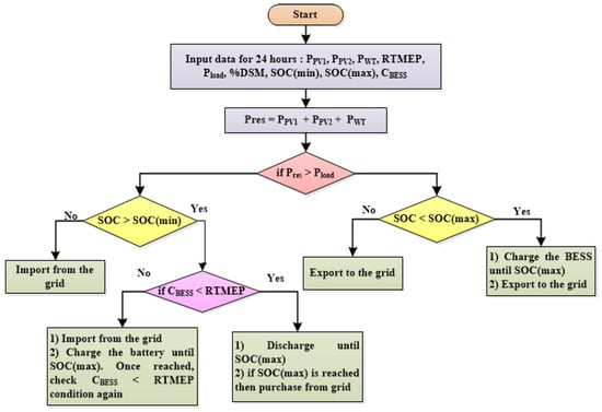
Figure 2.
EMS with PV, wind, and BESS integration in grid-connected microgrid.
The proposed EMS algorithm initially starts by comparing renewable power generation (‘Pres’) with the power demand of the load (‘Pload’) at each load level. If ‘Pres’ exceeds ‘Pload’—i.e., excess power may exist—then the present BESS SOC level is compared with SOC (max); if it is less than the SOC (max), then the BESS should be charged until the BESS reaches the SOC (max) level. If the excess power persists, then it can be sold to the utility grid. If ‘Pres’ is less than ‘Pload’—i.e., there is a deficit of power in the MGN—the stored energy in the BESS is utilized, if the SOC level is more than SOC (min). Under such a state, the cost of obtaining power from BESS (CBESS) and the utility grid based on the RTMEP is compared to decide the power to be drawn from the BESS or the utility grid., if CBESS is less than RTMEP, then the BESS will be allowed to supply the load demand until the BESS state reaches SOC (min). If CBESS is greater than RTMEP, then the utility grid will supply the load demand of the MGN and charge the BESS simultaneously until the BESS status reaches the SOC (max) level.
2.2.3. Demand Side Management Approach
In modern power systems, DSM is essential for managing load demand patterns and ensuring cost-efficient operation. One of the effective DSM implementation approaches is based on RTMEP, where the power purchasing price from the utility grid replicates real-time operating conditions, giving consumers a clear indication to shift their load when power is cheaper. It adopts a collaborative connection between utilities and customers which results in a more robust energy infrastructure that can adapt to variable load demand. This flexibility supports grid stability and renewable integration, aligning with the goals of sustainable energy use. Furthermore, a load in a network can be classified as an elastic load and an inelastic load. The composition of elastic and inelastic load components essentially decides the feasibility and benefits of DSM strategies. Elastic loads signify schedulable load consumption that can tolerate time-shifting without functional impact. Inelastic loads represent critical loads requiring immediate supply.
In this work, the MGN is assumed to be operated with elastic load (30%) and an inelastic load (70%). The 30% elastic load proportion considered in our study provides adequate flexibility for meaningful load reshaping (10%, 20%, 30% DSM scenarios) while maintaining MGN reliability [41]. The proposed DSM approach primarily focuses on the elastic load, which can be shifted from peak to off-peak hours without a change in total load demand of the MGN. The following steps are performed to implement the DSM strategies, i.e., at 10%, 20%, and 30% load shifting, with the aim of reducing the operational cost of the MGN.
Step 1: Input the load demand, PV1, PV2, wind generation, BESS capacity, and RTMEP;
Step 2: Calculate hourly elastic and inelastic loads;
Step 3: Input the % DSM to be considered;
Step 4: Based on the minimum operational cost function expressed in Equation (36), shift the given % of elastic loads from the peak hours to off-peak hours;
Step 5: The total load demand is estimated using Equation (39) after shifting the peak load demand.
2.3. Proposed Bi-Level Optimization Framework
This section presents the comprehensive methodology for integrating the top-level planning model and bottom-level operational optimization model. Figure 3 presents the comprehensive bi-level optimization framework that systematically integrates DG planning with operational energy management. The framework employs a hierarchical approach where the top-level model aims to minimize the technical losses through optimal DG placement and sizing, while the bottom-level model aims to minimize the operational costs of the MGN through intelligent energy resource dispatch through the proposed EMS integrated with DSM.
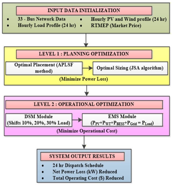
Figure 3.
Structure of Proposed bi-level optimization framework.
The bi-level optimization framework operates through four systematic stages:
Stage 1: System Initialization—Input MGN data, hourly load profiles, RTMEP, and PV and wind generation profiles. Initialize PV and wind DG and BESS technical specifications.
Stage 2: Top-Level Planning: Calculate APLSF for all nodes (Equation (16)) to identify optimal DG locations. Use the JSA to find the optimal hourly capacities for DG that minimize power losses (Equation (9)) while satisfying constraints (Equations (10)–(14)).
Stage 3: Bottom-Level Operation: Every hour, perform DSM strategy to reshape the load demand curve (Section 2.2.3). Use the EMS algorithm comparing renewable generation with load demand (Section 2.2.2). Share power optimization of PV, wind, BESS, and the grid using the JSA toward achieving an operating cost-minimizing (Equation (36)) while maintaining power balance (Equation (38)).
The strategy of DSM as discussed in Section 2.2.3 is implemented to modify the original load demand curve. The total load is divided into elastic load (30% of total) and inelastic load (70% of total). According to the level of DSM being measured (10%, 20%, or 30%), the corresponding percentage of elastic peak loads coinciding during hours is shifted to off-peak hours through JSA optimization. The objective function for DSM minimizes the cost of grid power procurement through the optimal offsetting of elastic loads to hours with lower RTMEP while complying with the constraint that the total daily energy consumption remains constant. The transformed load profile will then be input to the energy management strategy.
At each hour, the cost contributions for the operational expenditures from PV generation (), wind generation (), BESS operation (), and the utility grid power exchange () are calculated from their respective power output and bid rates. The 24 h operational cost will then be calculated as the accumulation of costs over all time periods. This cost metric will serve as one of the most important performance indicators that will serve to compare the different DSM strategies and validate the effectiveness of the proposed EMS.
Stage 4: Performance Evaluation: Assess technical performance (power loss reduction) and economic performance (24 h operational costs and cost savings) through 50 independent runs of the JSA with statistical analysis.
Such bidirectional coordination between top and bottom levels confirms that planning decisions are made considering operational realities, while operational strategies are optimized within constraints of installed capacities of energy resources to reach holistic techno-economic optimization.
2.4. Deterministic Framework and Uncertainty Considerations
2.4.1. Scope of Current Study
The proposed bi-level optimization framework employs a deterministic approach utilizing representative 24 h profiles for PV, wind generation, load demand, and RTMEP. These profiles are derived from typical operational patterns mentioned in the literature [4,5,55] providing a baseline scenario for validating algorithm and framework development.
2.4.2. Justification for Deterministic Approach
The deterministic modelling approach is justified as a vital fundamental step in evolving integrated bi-level optimization frameworks for the following reasons:
- Algorithm Validation and Proof-of-Concept: Deterministic frameworks enable clear assessment of optimization algorithm performance without the additional complexity of uncertainty propagation. This allows rigorous validation of the JSA’s convergence characteristics, solution quality, and computational efficiency for the proposed bi-level problem structure [18,19,20,32]. The 50 independent runs with statistical analysis confirm algorithmic robustness under deterministic conditions, establishing a foundation for stochastic extensions.
- Benchmark Establishment: Deterministic solutions provide performance benchmarks (power loss and operational costs minimization, optimal DSM thresholds) against which stochastic approaches can be compared. Many existing studies in MGN optimization similarly employ deterministic frameworks for initial methodology development [34,35,44,45], establishing comparative baselines in the literature.
- Computational Tractability: The bi-level optimization problem with 24 h scheduling horizon, various energy resources (PV, wind, BESS, grid), DSM implementation, and power flow constraints already presents significant computational complexity. The deterministic formulation enables tractable optimization within reasonable computational time (convergence achieved within 500 iterations).
- Representative Profile Approach: The use of representative profiles is a widely accepted practice in power system planning and operational studies [47,48,49]. These profiles capture typical operational patterns and provide meaningful insights for initial system design, capacity planning and operational strategy formulation. The high load factor profile (83%) employed in this work indicates a conservative worst-case scenario, ensuring that the proposed framework demonstrates effectiveness under challenging conditions.
2.4.3. Limitations of Deterministic Approach
The following limitations inherent in the deterministic modelling framework,
- Negligence of Forecast Error: Real-world renewable generation and load demand exhibit forecast errors typically ranging from ±10–25% depending on meteorological conditions [28]. The deterministic approach assumes perfect foresight of generation and demand patterns, which does not reflect operational reality where decisions must be made under uncertainty.
- Extreme Event Exclusion: Deterministic representative profiles may not adequately capture events such as rapid PV generation drops due to sudden cloud cover, volatility in wind generation due to wind gusts, and unforeseen load spikes.
- Conservative Operational Margins: To compensate for uncertainty in real-world implementation, deterministic solutions often require conservative operational margins (e.g., oversized BESS capacity, reserve generation capacity) that may not be economically optimal.
The deterministic framework developed in this study establishes the foundation for comprehensive stochastic extensions of the proposed optimization problem.
3. Modelling of PV and Wind Sources
The modelling of PV and wind energy systems to be deployed in the proposed MGN is performed using per-unit values over 24 h. The rated power for PV generation is taken as 5000 kW [4], and wind generation deployment is considered as 3500 kW operated with a 0.9 lagging power factor [56]. Figure 4 shows the power generation profile of PV and wind sources in per unit (p.u) [4,5] and the corresponding derived kW output for 24 h. The kW output of PV and wind sources is derived by multiplying p.u. values with the corresponding rated power of PV and wind sources considered. The capacity limits of PV and wind-based DG units, BESS, and their respective bid rates are presented in Table 2 [55].
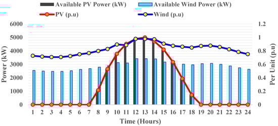
Figure 4.
Hourly power output of PV- and wind-based DG units in p.u. and in kW over 24 h.
Table 2.
Power capacity, bid rates of DG, and BESS units [4,5,55].
Modelling of Battery Energy Storage System
The simulation of the BESS unit evaluates its charging and discharging dynamics over a 24 h timeframe. The charging/discharging power for the ith BESS unit at hour t is presented by , respectively. The maximum allowable charging/discharging rates of BESS are constrained as specified in Equations (40) and (41):
The State of Charge (SOC) of the BESS is restricted within its defined operating range as specified in Equation (42):
In this work, the minimum SOC limit is taken as 20%, the maximum limit is considered as 80%, and the initial SOC is assumed to be 50%. When the BESS is charging/discharging, the SoC at the subsequent time step (t + 1) is updated using Equations (43) and (44) [41].
The analysis incorporates the charging and discharging efficiency of a BESS while ensuring the SOC remains within bounded limits as defined in Equation (42). The BESS charging and discharging efficiency () is taken as 80% [42]. The proposed EMS approach decides the BESS charging and discharging pattern based on generation and demand. During low-load-demand periods, if PV and wind generation exceed load, the BESS charges to store excess energy and during high-load-demand periods, if load exceeds generation, BESS discharges to meet the deficit load demand. The SOC management (20–80%) balances the cycle life of BESS with the need to accommodate load variations.
4. Result and Discussion
To verify the rationality of the proposed two-level optimization model proposed in this work, the IEEE 33-node radial distribution network is considered as a grid connected MGN. The 33-node MGN has 100 MVA as base power and 12.66 kV as an operating voltage [57]. The total load demand of the MGN at 100% load level is 3.715 MW and 2.300 MVAR, respectively. The hourly load demand of the MGN in p.u. values for 24 h is taken from [4]. The hourly RTMEP in (€ct/kWh) are taken from [55]. A typical daily load profile in kW is arrived at by the product of the hourly load in p.u. and the peak load demand of the MGN. The resulting load demand profile shows a high load factor, with sustained load demand above 3000 kW throughout the 24 h period. This heavy loading condition was specifically chosen to evaluate the strength of the proposed EMS under a constant operational stress scenario of the MGN. The hourly load profile and corresponding RTMEP (€ct/kWh) values are provided in Table 3. The utility grid RTMEP pricing typically includes demand charges based on peak load demand, making peak load management economically crucial. In our study, the Real-Time Market Energy Price (RTMEP) depicted in Table 3 shows that high loads coinciding with high RTMEP periods result in substantial operational costs, motivating implementation of the DSM strategies for efficient operation of the MGN with minimum operational cost.
Table 3.
Hourly load demand variation (kW) and RTMEP (€ct/kWh) over 24 h.
The specific load profile considered in this work (Table 3) exhibits a high load factor, with the minimum demand (about 3083 kW at hour 3) being around 83% of the peak load demand (3715 kW). This constant high baseload in the network creates a critical stress test for the proposed optimization framework, as it eliminates easy periods for BESS recharging and requires the EMS to manage available energy resources to prevent costly the utility grid dependency to satisfy the load demand. The load demand of the MGN considered is fluctuating narrowly between 3000 kW and 3715 kW. With a consistently high-load-demand profile of the MGN, the role of DSM becomes vital. Since with the minimal natural load valleys in the load demand profile, the proposed bi-level optimization is crucial to generate elasticity by shifting of elastic load up to 30%, thereby optimizing the usage of the PV and wind power generation during peak pricing periods.
4.1. Top-Level Planning Problem: Optimal Placement of PV and Wind Units
The optimal location of PV and wind DGs was decided based on the estimated APLSF values shown in Figure 5. Based on the highest APLSF value, the 6th and 28th nodes are selected for installing the two numbers of PV based DG units. A wind-based DG unit is placed in node number 3. The single-line diagram of the MG network with PV, wind, and BESS is depicted in Figure 6.
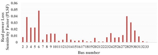
Figure 5.
APLSF at various nodes of the 33-node MGN.
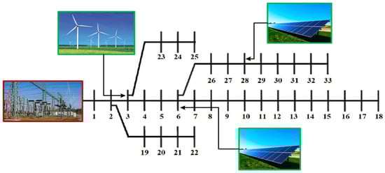
Figure 6.
The 33-node MGN with PV and wind-based DG units.
4.1.1. Impact of Optimal PV and Wind DG Units’ Integration on Power Loss
A backward/forward sweep-based power flow analysis is performed before and after the integration of PV- and wind-based DG units to study the impact of DG units on the power loss of the MGN. The power loss of 202.6853 kW was observed during the peak load demand (100% load level), which occurred at the 20th hour in the daily load demand curve before the integration of DG units. To determine the optimal sizing of PV and wind DG units, the JSA is applied with an objective of minimizing the power loss of the MGN at each load level of the daily load demand curve. The optimal rating of the PV and wind units to be placed in the MGN at each load level and the associated power loss of the MGN are depicted in Figure 7.
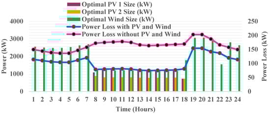
Figure 7.
JSA-based optimal sizing of PV and wind power at each load level with variation in power loss.
The tuning parameters for the JSA for the proposed optimization problem considered are as follows: number of populations = 30; distribution coefficient (β) = 3; motion coefficient (δ) = 0.1; number of iterations = 500. For PSO, the learning coefficients (C1, C2) are taken as 2.05, and ωmin and ωmax as 0.4 and 0.9, respectively. Similarly, for OOA, random numbers ( are chosen between [0, 1] and [1, 2].
Figure 8 depicts the convergence characteristics of the Jellyfish Search Algorithm (JSA), Particle Swarm Optimization (PSO), and Osprey Optimization Algorithm (OOA) applied to the top-level planning problem of minimizing power losses through optimal DG sizing at four representative hours (1st, 8th, 15th, and 22nd) representing diverse loading conditions across the 24 h operational cycle. Across all four loading scenarios depicted in Figure 9, the JSA demonstrates consistently faster convergence to optimal or near-optimal solutions compared to PSO and the OOA. The JSA’s smooth convergence via adaptive TCM avoids premature convergence observed in PSO and the OOA.
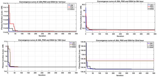
Figure 8.
Convergence curve of the objective function (power loss) at 1st, 8th, 15th, and 22nd hour loading condition using JSA, PSO, and OOA.
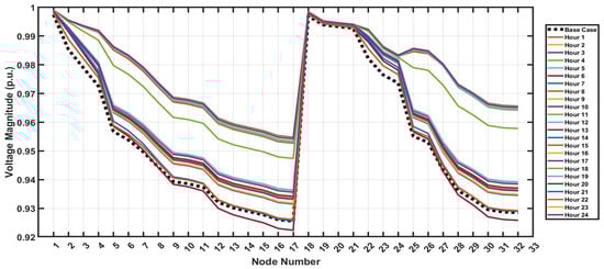
Figure 9.
Hourly voltage profiles of 33-node MGN with JSA-optimized PV/wind integration.
The voltage profiles demonstrate that all node voltages are maintained within the permissible operating limits of 0.9 p.u. to 1.1 p.u. (±10% of nominal voltage) as specified in Equation (14), thereby validating the effectiveness of the APLSF-based DG placement methodology. Table 4 depicts the reduction in power loss of the MGN at different loading scenarios. The power loss reduction is most significant during low-to-moderate load conditions (48–58%) due to optimal current flow redistribution through strategic DG placement in the network. Even at peak load condition of the MGN, substantial loss reduction (24.04%) is achieved.
Table 4.
Power loss reduction through optimal DG placement.
4.1.2. Statistical Results
To evaluate the robustness of the JSA, PSO, and OOA, each algorithm was executed for 50 independent runs and their statistical results are summarized in Table 5. Various statistical metrics including mean fitness, minimum fitness, maximum fitness, standard deviation, median and average computational time are computed to assess consistency in the optimization process. The statistical results depicted in Table 5 indicate that the JSA consistently provides the minimum standard deviation and computation time, over PSO and the OOA showing its robustness across multiple runs to arrive at the best solution.
Table 5.
Statistical analysis of the JSA, PSO, and OOA at 100% load level at peak hour (13th hour).
This top tier planning model has determined the most appropriate locations and sizes for PV- and wind-based DG units. The following sections describe the operational phase of the MGN where an optimization model at a bottom level is used to minimize operational costs through the implementation of coordinated EMS and DSM strategies.
4.2. Bottom-Level Operational Results
Renewable-based microgrids face the challenge of meeting the load demand despite variable and uncertain generation from PV and wind sources. The PV generation peaks during midday (9th–17th h in our study), while wind generation patterns often do not correlate with load peaks. Our simulation results reveals that peak load occurs at the 20th h (3715 kW), while maximum PV generation happens at the 9th h, making a temporal mismatch that necessitates cautious planning of PV, wind DGs, placement, and operational strategies. This discrepancy is the key reason for BESS integration in the MGN and DSM becoming critical. The magnitude and time-based variation in load demand directly decide the required capacity of PV and wind-based units and BESS. In our case study, with a sustained load variation over a 24 h period, the PV- and wind-based DG units must be sized not just for average load but considering peak demand and generation-load demand coincidence factors. The BESS capacity must accommodate charging during low-load and peak generation periods and discharging during high load during low generation periods. Our bi-level optimization approach explicitly addresses this by optimizing PV, wind, and BESS sizing at different load levels (not just peak) using hourly load profiles, ensuring efficient operation of the MGN across the entire daily load curve. In this work, the optimal location of PV, wind, and BESS is selected based on the APLSF values estimated using Equation (16). Based on the estimated APLSF values, the 6th, 28th node, and 3rd node are chosen for placing two numbers of PV units and a wind-based DG unit. A BESS is placed at 29th node. Figure 10 depicts the single-line diagram of a grid-connected MGN with PV, wind, and BESS.
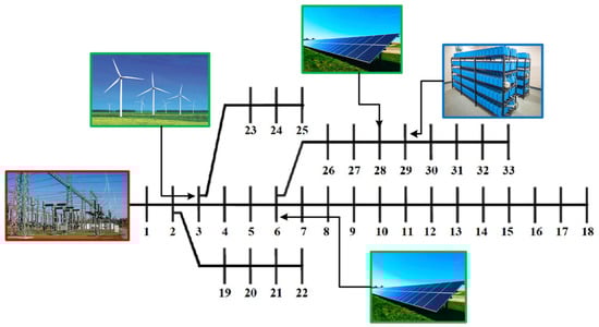
Figure 10.
The 33-node MGN with PV- and wind-based DG units and BESS.
The following four test scenarios are considered to investigate the impact of proposed EMS and DSM strategies on the MGN planning with the integration of PV, wind, BESS, and the utility grid.
- Test Case 1—MGN with PV, wind with EMS, and without considering DSM.
- Test Case 2—MGN with PV, wind, BESS with EMS, and consideration of 10% DSM.
- Test Case 3—MGN with PV, wind, BESS with EMS, and consideration of 20% DSM.
- Test Case 4—MGN with PV, wind, BESS with EMS, and consideration of 30% DSM.
4.2.1. Test Case 1: EMS with PV, Wind, and BESS Without DSM Implementation
Simulation results for Test Case 1 are depicted in Figure 11, in which during hours 1 to 8, the installed renewable power is insufficient to meet the load demand, resulting in the utility grid supplying the deficit power while the BESS remains ideal, as the cost of energy from BESS is greater than the RTMEP of the grid power in that period. In the 11th, 14th, 16th, 18th, 21st, and 23rd hours, PV and wind generation are insufficient to meet the load demand. During this period, the proposed EMS utilizes the BESS to discharge until SOC (min) due to its lower cost of energy supply compared with the RTMEP of the utility grid power. During hours 12, 15, 17, 20, and 22, BESS is under SOC (min) and there is insufficient generation from PV and wind sources; the proposed EMS schedules the utilization of grid power to meet the load demand and initiate BESS charging during this period. The charging and discharging pattern of the BESS, scheduled by the proposed EMS, is adaptive based on the RTMEP of the grid power. The proposed EMS algorithm decides every operational decision, whether to charge/discharge the BESS, and the import/export grid power based on the instantaneous comparison between total renewable generation and load demand.

Figure 11.
Power sharing scenario of PV, wind, and BESS without the consideration of DSM (Test Case 1).
During the peak power generation (9th h), the optimal power injection from the PV and wind units is 2060.47 kW (1260.64 kW from PV1, 799.83 kW from PV2) and 1266.81 kW, respectively. The total generation of 3327.28 kW from PV and wind DG units is insufficient to meet the load demand during that period (3466.095 kW). The deficit of 138.815 kW is supplied from the BESS to satisfy the load demand during this hour. This instance reflects the proposed EMS’s ability to dynamically adjust the power sharing based on the availability of power generation from the renewable-based DG units. The operational cost (in 9th hour) for power injection from the PV- and wind-based DG units contribute about €ct 5324.25 and €ct 1359.28, respectively. The utility grid contributes at a slightly higher cost of approximately €ct 52.7497. The total operational cost for the 24 h period amounts to €ct 114,113.22.
4.2.2. Test Case 2: EMS with PV, Wind, and BESS After 10% DSM Implementation
In Test Case 2, with the implementation of the EMS strategy with 10% DSM, the power sharing between the PV, wind, BESS, and the utility grid at each hour is summarized in Figure 12. In this test case, 10% of the elastic peak demand is shifted to off-peak hours with the objective of minimizing the operational cost. The total operational cost in Test Case 2 decreased to €ct 112,477.5106, which, when compared to Test Case 1 (€ct 114,113.22), yielded a saving of €ct 1635.71003. During the 9th hour, in which the renewable contribution is maximum, the power injection from the PV and wind-based renewable sources is 2060.47 kW (1260.64 kW from PV1, 799.83 kW from PV2) and 1266.81 kW, respectively. The total power generation during that period (3327.28 kW) is insufficient to meet the load demand (3362.11215 kW). The proposed EMS schedules the deficit power of 34.83215 kW from the BESS to satisfy the load demand. The discharging of the BESS unit is scheduled by the proposed EMS due to higher RTMEP of the grid power during that period.
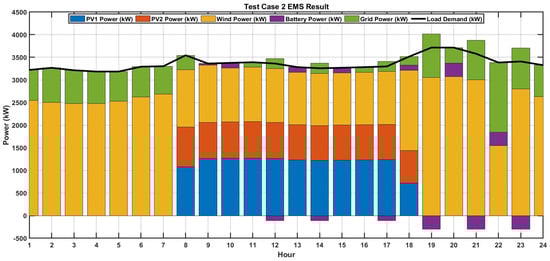
Figure 12.
Power sharing scenario of PV, wind, and BESS with 10% DSM (Test Case 2).
4.2.3. Test Case 3: EMS with PV, Wind, and BESS After 20% DSM Implementation
In Test Case 3, with 20% of the elastic peak demand moved to off-peak hours, the power sharing between the PV, wind, BESS, and the utility grid is summarized in Figure 13. Similar to Test Case 1, in Test Case 3, during the 9th hour period, the power injection from the PV units and wind DG is 2060.47 kW (1260.64 kW from PV1; 799.83 kW from PV2) and 1266.81 kW, respectively. The total generation of 3327.28 kW is sufficient to meet the load demand during that period (3258.129 kW). The excess of 69.151 kW is used to charge the BESS. In Test Case 3, the estimated total operational cost is €ct 110,917.04, yielding a savings of €ct 3196.1776 when compared to Test Case 1. Over the 24 h load demand variation, the load demand is met economically with the aid of optimal power injection from PV- and wind-based DG units, BESS, and the utility grid.
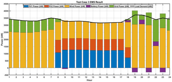
Figure 13.
Power sharing scenario of PV, wind, and BESS with 20% DSM (Test Case 3).
4.2.4. Test Case 4: EMS with PV, Wind, and BESS After 30% DSM Implementation
The hourly power sharing among the energy resources for Test Case 4 is depicted in Figure 14. Similar to the previous test case analysis, the peak power generation from the PV and wind sources during the 9th hour, and the optimal power injection from the PV and wind DG units is 2060.47 kW (1260.64 kW from PV1 and 799.83 kW from PV2) and 1266.81 kW, respectively. The total generation is 3327.28 kW, which is sufficient to meet the load demand during that period (3154.14645 kW). The proposed EMS schedules the excess generation of 173.13 kW is to charge the BESS (150 kW), and the remaining 23.13 kW is exported to the utility grid. In Test Case 4, the estimated total operational cost is €ct 1,11,077.78, and a saving of €ct 3035.43708 is realized when compared to Test Case 1.
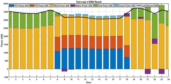
Figure 14.
Power sharing scenario of PV, wind, and BESS with 30% DSM (Test Case 4).
Table 6 compares the performance of four DSM implementation levels, revealing critical insights into optimal microgrid operation. Test Case 3 (20% DSM) exhibits superior performance in terms of maximum possible operational cost savings of €ct 3196.18 (2.80% reduction) along with the highest grid dependency reduction during peak hours (46.75%). It is, however, interesting to note that Test Case 4 (30% DSM) shows unexpected results since the maximum load was shifted to peak times (2772.43 kW versus 1848.29 kW) but still incurs higher operational costs of approximately €ct 111,077.78, which suggests that reducing loads beyond a certain optimum level would be counterproductive.
Table 6.
Comparative performance across DSM strategies.
This phenomenon happens as pushing demand aggressively into many off-peak hours where the generation of renewables is less, which creates increased reliance on BESS discharge and expensive utility grid imports when BESS SOC constraints are active. These findings reveal that DSM effectiveness is non-monotonic, identifying 20% as the optimal load shifting level that balances cost reduction, grid dependency minimization, and practical feasibility.
The effectiveness of DSM directly depends on the load characteristics of the MGN with predominantly inelastic loads cannot benefit significantly from time-based RTMEP pricing or load-shifting strategies. Our results demonstrate that 20% DSM (shifting 6% of total peak load) achieves the best economic performance (€ct3,196.18 savings), when the peak load of 6% is shifted to benefit from time-varying electricity prices validating that load characteristics and DSM strategy must be carefully matched. Figure 15 illustrates the impact of DSM strategies on reducing operational costs and power loss of the MGN across different test cases analyzed, emphasizing the effectiveness of DSM in shifting peak load without compromising the total load demand of the MGN.

Figure 15.
Operational cost and peak load power loss variation with different test cases.
- Peak Saving Performance Across DSM Strategies:
Table 7 presents detailed peak hour load management metrics including total peak hour load shifted, peak hour grid imports costs, grid dependency reduction percentages, load profile variance, and Energy Autonomy Index across all test cases. Table 8 provides comparative key performance indicators across economic savings, peak hour grid dependency reduction, load profile smoothing, total peak load shifted, Energy Autonomy Index, and peak hour load, clearly demonstrating that Test Case 3 achieves the optimal performance over other Test Cases.
Table 7.
Peak hour load management and grid dependency metrics across DSM strategies.
Table 8.
Key performance indicators.
The comprehensive peak shaving analysis across DSM strategies revealing Test Case 3 (20% DSM) as the optimal configuration achieving maximum economic savings (€ct3,196.18, 2.80% reduction), highest peak hour grid dependency reduction (46.75%), and maximum Energy Autonomy Index (0.769). Despite Test Case 4 (30% DSM) shifting more peak load (2772.43 kW vs. 1848.29 kW) and achieving a 9% physical peak reduction, it paradoxically delivers 3.71% (43.04%) lower grid dependency reduction.
- Implicit Peak Shaving Through RTMEP-DSM Mechanism:
In the proposed approach, the DSM optimization naturally shifts elastic loads away from high-price peak periods to low-price off-peak periods; minimizing cost requires reducing expensive peak-hour grid imports, which simultaneously achieves peak load reduction. Test Case 3 achieves a 46.75% reduction in peak-hour grid dependency (from €ct 6439.21 to €ct 3429.13), the highest among all scenarios with physical peak load reduced by 6%. Despite Test Case 4 achieving maximum physical peak reduction (9%), its peak-hour grid dependency reduction (43.04%) is 3.71 percentage points worse than Test Case 3. While Test Case 4 achieves the largest absolute peak reduction, it suffers from temporal misalignment (excessive off-peak load concentration) and BESS constraint violations, resulting in inferior economic and grid dependency performance compared to Test Case 3’s strategic peak shaving. Thus, the cost-centric objective function implicitly optimizes peak shaving because the RTMEP structure incentivizes load reduction during peak-price hours. This analysis reveals non-monotonic DSM performance with marginal economic benefit and peak shaving efficiency. The critical decoupling between peak load reduction (Test Case 4: 9%) and economic performance (Test Case 3: €ct 3196) demonstrates that optimal DSM targets strategic load reshaping for renewable-load temporal alignment rather than maximum peak minimization. These findings validate 20% DSM as the system specific optimal threshold balancing technical, economic, and operational objectives within the 70–80% energy autonomy optimal range.
Figure 16a–c demonstrate that all three DSM implementation strategies maintain node voltages within the allowable operating range of 0.9 p.u. to 1.1 p.u. (±10% of nominal voltage) throughout the 24 h operational period. This validates that the proposed integrated EMS-DSM optimization framework achieves economic objectives (operational cost minimization) without compromising voltage stability requirements.
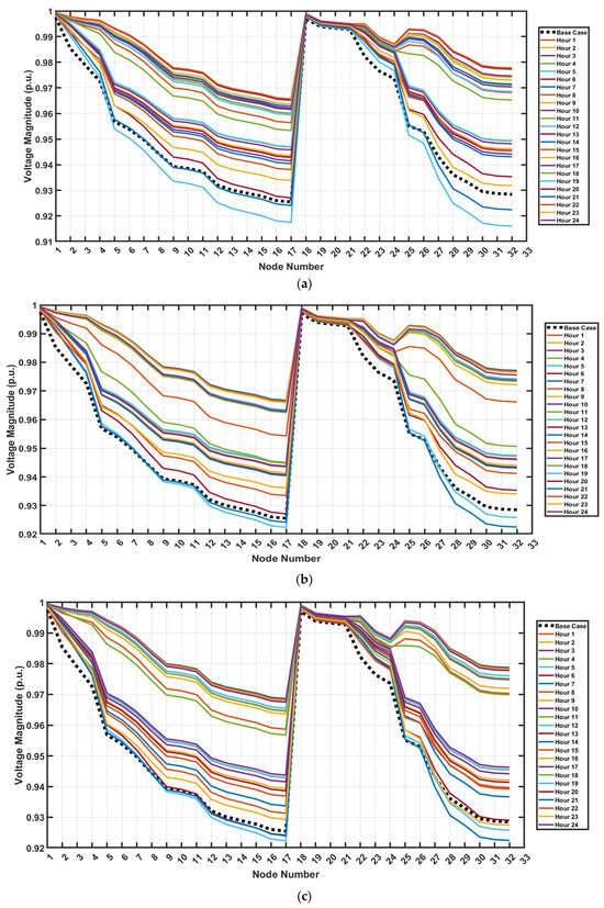
Figure 16.
(a) Hourly voltage profiles of 33-node MGN with JSA-based optimized PV, wind, and BESS (Test Case 2). (b) Hourly voltage profiles of 33-node MGN with JSA-based optimized PV, wind, and BESS (Test Case 3). (c) Hourly voltage profiles of 33-node MGN with JSA-based optimized PV, wind, and BESS (Test Case 4).
4.3. Statistical Analysis
To evaluate the robustness of the JSA, PSO, and OOA based DSM load shifting approaches and to obtain the optimal solution, three distinct test cases were executed with 50 independent runs using random population seeds. The statistical results including the maximum, minimum, mean, and standard deviation of the fitness function (operational cost) of the proposed optimization problem are summarized in Table 9. These metrics enable a comprehensive comparison of the test cases and validate the statistical performance of the JSA-based DSM over PSO and the OOA across different scenarios. Figure 16a–c represent the convergence behaviour of the JSA, PSO, and OOA to achieve the optimal operational cost function of the different test cases considered.
Table 9.
Statistical analysis of the JSA-based DSM approach at 100% load level over 50 independent runs.
Figure 17a–c present a comprehensive comparative analysis of the JSA, PSO, and OOA applied to the bottom level operational optimization problem (Equation (37)) across three DSM implementation strategies. The convergence curves demonstrate that the JSA consistently outperforms both PSO and the OOA across all three test cases in terms of convergence speed, solution quality, and robustness. This comprehensive superiority validates the selection of the JSA as the primary optimization technique for both top-level planning (power loss minimization) and bottom-level operation (cost minimization), as supported by statistical analysis with 50 runs (Table 5 and Table 9), while convergence curves (Figure 8 and Figure 17) and computational time metrics conclusively validate the JSA’s superiority for the proposed bi-level framework.
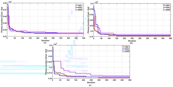
Figure 17.
JSA, PSO, and OOA convergence curves for (a) Test Case 2, (b) Test Case 3, and (c) Test Case 4.
Figure 18 shows the comparative operational analysis across DSM scenarios showing the following: (a) hourly load demand profiles after DSM implementation; (b) BESS State-of-Charge trajectories; (c) grid power import patterns.
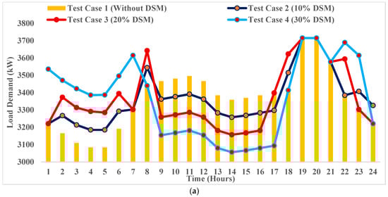
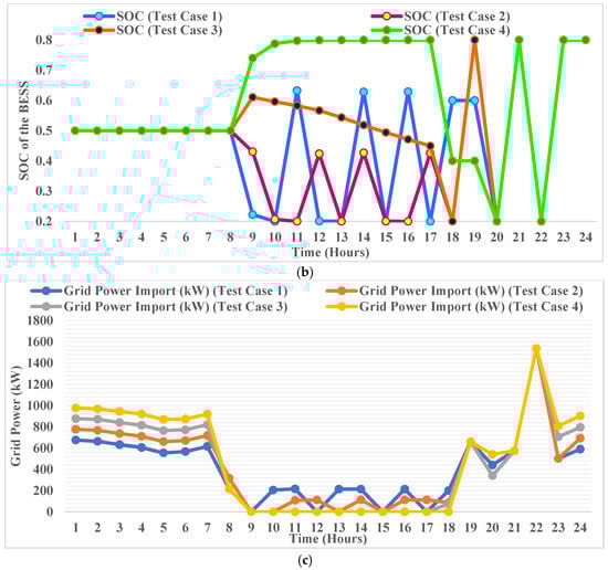
Figure 18.
(a) Load shifting patterns for all test cases. (b) SOC trajectories of the BESS for all test cases. (c) Grid power imported for all test cases.
4.4. Comprehensive Mechanistic Analysis of DSM
The three interrelated mechanisms that drive non-monotonic DSM performance are observed in Figure 18a–c.
4.4.1. Temporal Misalignment
Figure 18a depicts 24 h load demand curves showing exactly where loads are shifted in each DSM scenario, revealing the critical temporal alignment differences between the test cases considered. The analysis reveals that Test Case 3 (20% DSM) strategically targets 51% of shifted loads (940 kW) to PV peak hours (7–13), realizing near-perfect renewable-load temporal coincidence. In contrast, Test Case 4 (30% DSM) shifts only 14% (400 kW) to PV peak hours while shifting 61% (1680 kW) to nighttime deficit hours (1–8) when PV output is zero and wind delivers only 800–1100 kW. This temporal misalignment forces Test Case 4 to import supplementary power from the utility grid during off-peak hours compared to Test Case 3’s strategic way of shifting the load.
4.4.2. BESS Constraint Violation
Figure 18b illustrates hour-by-hour SOC dynamics, explicitly demonstrating SOC constraint violations in Test Case 4 (30% DSM) versus optimal SOC management in Test Case 3 (20% DSM). The SOC constraint violations directly influence the Energy Autonomy Index, which reduces from 0.769 (Test Case 3) to 0.752 (Test Case 4), a 2.2% degradation indicating reduced local resource utilization effectiveness.
4.4.3. Grid Dependency Patterns
Figure 18c quantifies the utility grid dependency patterns across 24 h, quantifying the “double penalty” effect where Test Case 4 experiences both increased off-peak grid imports and reduced peak-hour profits. In Test Case 3, 46.75% peak-hour utility grid dependency reduction is attained (€ct 3010.08 savings), reducing peak hour utility grid import cost from €ct 6439.21 (baseline) to €ct 3429.13. In Test Case 4, the total grid cost of €ct 3667.89 (43.04% reduction) is higher than Test Case 3 despite shifting more load.
4.5. Novelty of Proposed Framework
The key contributions of the proposed optimization framework are as follows:
- Integrated Bi-Level Optimization: The framework jointly coordinates optimal planning and operation of MGN attaining combined benefits compared to independently executed optimization processes.
- The result outcomes validate that a 20% DSM threshold level is identified as optimal, which reveals that the DSM obtains a 2.80% cost reduction and 47% decrease in peak-hour utility grid dependency.
- RTMEP-responsive coordination: Hour-by-hour dynamic comparison of vs. RTMEP enables adaptive and economically optimized power sharing among PV, wind, BESS, and the utility grid.
From a practical perspective, finding an optimal DSM threshold has significant implications for MGN operators and DSM program designers. The results prove that the relationship between load shifting magnitude and economic benefit follows a concave function with a distinct maximum, rather than the monotonically rising relationship often assumed in simplified models. This finding advocates that DSM programs should be designed with explicit threshold constraints rather than maximizing load shifting percentage without boundaries. For the specific MGN configuration studied (33-node MGN), the optimal elastic load shifting is approximately 6% of peak demand, yielding maximum economic benefit without compromising operational reliability or renewable energy utilization.
While the proposed bottom-level operational optimization clearly reduces operational costs, the framework inherently achieves multi-objective benefits through the integrated EMS-DSM mechanism.
The proposed optimization framework is designed to address multiple interrelated objectives that jointly enhance the economic, technical, and environmental performance of the MGN. From an economic perspective, the primary objective is the reduction in operational costs through optimal resource scheduling. This includes RTMEP responsive BESS charging/discharging decisions, as well as the optimization of the utility grid power import/export in response to dynamic RTMEP variations. Additionally, the proposed framework implicitly achieves peak saving by reducing peak load demand through elastic load shifting from peak to off-peak hours. This results in a considerable reduction in peak grid imports with a reduction of 46.75% in Test Case 3.
From a technical viewpoint, the top-level objective emphasis augmenting MGN performance through power loss reduction and voltage profile regulation. Optimal placement and sizing of PV- and wind-based DG units lead to a substantial reduction in power losses by 24.04 at peak load condition, while concurrently improving the voltage profile across the MGN and maintaining voltage levels within the tolerable ±10% limits.
Finally, the proposed framework implicitly helps environmental sustainability by maximizing renewable energy utilization through coordinated scheduling of PV, wind, and BESS resources. Reduced dependence on grid power lowers the need for fossil fuel-based generation, thereby contributing to a reduced carbon footprint. The integration of intelligent demand-side participation further strengthens the MGN ability to operate in an environmentally responsible and energy-efficient manner. The harmonious achievement of these objectives validates the effectiveness of the proposed integrated bi-level optimization framework, demonstrating that cost-oriented optimization under appropriate constraints (DSM, BESS management, renewable integration) naturally aligns with peak saving, technical efficiency, and environmental sustainability.
4.6. Limitations of the Proposed Deterministic Approach and Future Research Directions
The results presented in this study (24.04% power loss reduction, €ct 3196.18 cost savings, 46.75% peak grid dependency reduction) represent the baseline performance under deterministic representative profiles. While the 20% DSM level proves an optimal operating scenario for the MGN considered in this work, future work should explore adaptive DSM approaches that dynamically alter the percentage of load shifting based on prevailing situations. The optimal threshold level of DSM may depend on different network topologies, penetration levels of RES, load demand profiles, and the price structure of RTMEP.
While our analysis identifies 20% DSM as optimal for the studied configuration, we acknowledge that the optimal threshold is system-specific and depends on (i) the ratio of renewable generation capacity to peak load; (ii) BESS energy capacity relative to daily load variation; (iii) the temporal pattern of RTMEP relative to renewable generation profiles, and (iv) the elastic/inelastic load composition. Future work should explore the functional relationship between these system parameters and optimal DSM thresholds.
In real-world application under uncertainty in renewable generation and load demand, these performance metrics would exhibit variability. While the current deterministic approach validates the proposed bi-level optimization methodology and JSA effectiveness, comprehensive stochastic modelling represents an essential extension for practical implementation in real-world MGN operating under uncertainty.
Future research will address the implementation of PV and wind generation uncertainty quantification through historical irradiance data analysis to derive probability distributions (e.g., Beta distribution for solar irradiance, accounting for cloud transients, snow coverage), seasonal variation patterns affecting uncertainty magnitude, accounting for wind speed stochasticity using Weibull distribution characterization, ramping event probability, and the impact on operational scheduling. Similarly, for load demand uncertainty modelling, considering weather-sensitive loads such as heating, cooling loads with temperature correlation, stochasticity in consumer behaviour in elastic load response during DSM, variations in load demand patterns during holidays, and industrial operational schedules which reflect the real-world operating scenario of the MGN will be necessary.
While the current study preserves BESS health through strict SOC limits (20–80%) and bid-rate modelling, an integrated BESS life loss cost model would provide a more granular view of the long-term economic trade-offs in DSM.
The current study demonstrates that cost minimization implicitly achieves peak saving benefits, and explicit multi-objective formulations could provide enhanced flexibility for system operators with diverse priorities. The integration of explicit multi-objective optimization would enable customizable MGN operation strategies tailored to specific stakeholder priorities, regulatory requirements enhancing the practical appropriateness of the proposed optimization framework across diverse deployment scenarios.
These impacts highlight the importance of the stochastic optimization extensions, which will provide assurances for probabilistic performance and risk-adjusted operational approaches. However, the deterministic method establishes the foundational methodology, algorithmic validation, and baseline performance benchmarks essential for successive stochastic development of the proposed optimization problem.
5. Conclusions
This article presents a comprehensive JSA-based bi-level optimization framework for MGN energy management that combines PV, wind, and BESS in a grid-connected MGN with twin objectives: reducing power loss through optimal DG placement and sizing, and minimizing operational costs through intelligent scheduling of energy resources with DSM. The proposed approach has been validated through extensive simulations on the IEEE 33-node MGN, demonstrating several significant contributions. The integrated bi-level optimization framework simultaneously coordinates planning-level decisions (DG allocation, BESS sizing) with operational-level strategies (optimal scheduling of PV, wind, BESS units and the utility grid, DSM implementation), achieving synergistic benefits unachievable through independent optimization processes. The APLSF-based DG placement combined with JSA optimization realizes substantial power loss reduction ranging from 48.02% at minimum load to 24.04% at peak load while maintaining a voltage profile within allowable limits throughout 24 h operation. A critical finding is the identification of an optimal DSM threshold at 20%, which achieves maximum operational cost savings of €ct 3196.18 (2.80% reduction) and highest peak-hour grid dependency reduction (46.75%), revealing that DSM effectiveness follows a non-monotonic relationship where aggressive load shifting beyond optimal thresholds (30% DSM) paradoxically delivers inferior economic performance due to temporal misalignment between shifted loads and PV- and wind-based renewable generation patterns, BESS constraint violations, and increased off-peak grid dependency. The mechanistic analysis identifies three interrelated factors governing DSM performance: temporal alignment (Test Case 3 strategically shifts 51% of elastic loads to PV peak hours vs. Test Case 4 shifting only 14%), BESS constraint management (optimal SOC trajectories vs. constraint violations), and utility grid dependency patterns (€ct 3429.13 peak-hour grid cost vs. €ct 3667.89). Statistical analysis over 50 independent runs confirms the JSA’s dominance over PSO and the OOA, achieving minimum standard deviation (0.00017 for planning, 36.51 for operation) and fastest computational time (18.69 s vs. 36.67 for PSO and 82.70 for OOA), with convergence characteristics demonstrating effective exploration–exploitation balance through adaptive TCM.
The practical significance extends across technical, economic, and operational domains with broader implications for sustainable MGN deployment. Technically, the framework achieves a power loss reduction from 202.69 kW to 153.95 kW at peak conditions while maintaining voltage profiles within tolerable ranges. Economically, the 20% DSM strategy delivers maximum cost savings while achieving a 46.75% reduction in peak-hour grid dependency and Energy Autonomy Index of 0.769, demonstrating optimal local resource utilization. The cost-centric objective function inherently attains peak shaving through the RTMEP structure that incentivizes load reduction during peak-price hours, validating that economic optimization and peak demand management are synergistic objectives. The finding reveals that optimal DSM targets strategic load reshaping for renewable-load temporal alignment rather than maximum peak minimization and provides actionable guidance for DSM program design, suggesting that DSM programs should employ explicit threshold constraints tailored to system-specific characteristics (renewable capacity-to-peak load ratio, BESS capacity relative to daily variation, RTMEP temporal patterns, elastic/inelastic load composition). While this deterministic framework establishes robust algorithmic validation and performance benchmarks, future research should address important extensions including stochastic modelling incorporating probabilistic characterization of renewable generation and load uncertainty with forecast error quantification, multi-microgrid coordination frameworks enabling energy trading and reserve sharing through distributed optimization, advanced BESS degradation modelling for explicit life-cycle cost optimization, adaptive DSM approaches using machine learning approaches to dynamically adjust load shifting based on real-time forecasts, explicit multi-objective formulations providing Pareto-optimal solutions balancing conflicting objectives, real-world pilot deployments for validation under actual operational conditions, integration with electric vehicle charging infrastructure, and regulatory framework design for appropriate incentive mechanisms. In conclusion, the integrated bi-level optimization framework, optimal DSM threshold identification, mechanistic performance analysis, and JSA algorithmic validation advance both the theoretical state-of-the-art and practical implementability of intelligent MGN energy management. As power systems transition toward increased renewable penetration and active consumer participation, this work provides critical methodological foundations and operational insights for achieving reliable, economical, and sustainable MGN operation harmonizing technical performance, economic efficiency, and environmental responsibility.
Author Contributions
Conceptualization, V.N. and M.K.; methodology, V.N. and M.K.; software, V.N.; validation, M.K., R.T. and W.-W.K.; writing—original draft preparation, V.N. and M.K.; writing—review and editing, R.T., W.-W.K. and Z.W.G.; visualization, R.T.; supervision, M.K. and Z.W.G.; funding, W.-W.K. and Z.W.G. All authors have read and agreed to the published version of the manuscript.
Funding
This work was supported by the Korea Institute of Energy Technology Evaluation and Planning (KETEP) and the Ministry of Trade, Industry & Energy (MOTIE) of the Republic of Korea (RS-2023-00236325). This work was also supported by the Gachon University research fund of 2025 (GCU-202503130001).
Data Availability Statement
Dataset is available upon request from the authors.
Acknowledgments
The authors would like to express their gratitude to the management of SASTRA Deemed to be University for providing Renewable Energy Lab facilities.
Conflicts of Interest
The authors declare no conflicts of interest.
Abbreviations
The following abbreviations are used in this manuscript:
| PV | Photovoltaic |
| BESS | Battery Energy Storage System |
| MGN | Microgrid Network |
| EMS | Energy Management System |
| DSM | Demand Side Management |
| RTMEP | Real-Time Market Energy Price |
| JSA | Jellyfish Search Algorithm |
| DG | Distributed Generation |
| RES | Renewable Energy Sources |
| PSO | Particle Swarm Optimization |
| HS | Harmony Search |
| AGTO | Artificial Gorilla Troops Optimizer |
| HBA | Honey Badger Algorithm |
| TCM | Time Control Mechanism |
| GA | Genetic Algorithm |
| DE | Differential Evolution |
| APLSF | Active Power Loss Sensitivity Factor |
| TCF | Time Control Function |
| SOC | State Of Charge |
References
- Babagheibi, M.; Jadid, S.; Kazemi, A. Distribution locational marginal pricing for congestion management of an active distribution system with renewable-based microgrids under a privacy-preserving market clearing approach and load models. Sustain. Energy Grids Netw. 2022, 32, 100935. [Google Scholar] [CrossRef]
- Shirmardi, S.A.; Joorabian, M.; Barati, H. Flexible–reliable operation of green microgrids including sources and energy storage-based active loads considering ANFIS-based data forecasting method. Electr. Power Syst. Res. 2022, 210, 108107. [Google Scholar] [CrossRef]
- Youssef, H.; Kamel, S.; Hassan, M.H. Smart home energy management and power trading optimization using an enhanced manta ray foraging optimization. Sci. Rep. 2023, 13, 22163. [Google Scholar] [CrossRef] [PubMed]
- Pompern, N.; Premrudeepreechacharn, S.; Siritaratiwat, A.; Khunkitti, S. Optimal placement and capacity of battery energy storage system in distribution networks integrated with PV and EVs using metaheuristic algorithms. IEEE Access 2023, 11, 68379–68394. [Google Scholar] [CrossRef]
- Amir, A.; Shareef, H.; Awwad, F. Energy management in a standalone microgrid: A split-horizon dual-stage dispatch strategy. Energies 2023, 16, 3400. [Google Scholar] [CrossRef]
- Anand, M.P.; Ongsakul, W.; Singh, J.G.; Sudhesh, K.M. Optimal allocation and sizing of distributed generators in autonomous microgrids based on LSF and PSO. In Proceedings of the International Conference on Energy Economics and Environment (ICEEE), Bangkok, Thailand, 11–13 March 2015. [Google Scholar]
- Tahir, M.J.; Abu Bakar, B.; Alam, M.; Su’ud, M.M. An LSF-based DG placement approach for power losses minimization of the radial distribution network. In Proceedings of the 13th International Conference on Mathematics, Actuarial Science, Computer Science and Statistics (MACS), Bandung, Indonesia, 26–27 October 2019. [Google Scholar]
- Brahmantino, N.S.; Banjar-Nahor, K.M.; Widjaja, C.D.; Hariyanto, N. Development of a new LSF-based algorithm for optimal placement and sizing of distributed VRE. In Proceedings of the IEEE PES Innovative Smart Grid Technologies Asia (ISGT Asia), Brisbane, Australia, 5–8 December 2021. [Google Scholar]
- Diab, A.A.Z.; Mahmoud, F.S.; Sultan, H.M.; El-Sayed, A.-H.M.; Ismeil, M.A.; Kamel, O.M. Various optimization algorithms for efficient placement and sizing of photovoltaic distributed generations in different networks. PLoS ONE 2025, 20, e0319422. [Google Scholar] [CrossRef] [PubMed]
- Geem, Z.W.; Kim, J.H.; Loganathan, G.V. A new heuristic optimization algorithm: Harmony search. Simulation 2001, 76, 60–68. [Google Scholar] [CrossRef]
- Ali, S.M.; Babu, P.S.; Gurusekhar, B. Reconfiguration with simultaneous DG installation to improve the voltage profile in the distribution network using the harmony search algorithm. Bull. Electr. Eng. Inform. 2015, 4, 257–273. [Google Scholar] [CrossRef]
- Roy, K.; Bansal, S.K.; Bansal, R.C. Performance enhancement of radial distribution system with optimal DG allocation. Int. J. Model. Simul. 2025, 45, 245–263. [Google Scholar] [CrossRef]
- Elseify, M.A.; Kamel, S.; Abdel-Mawgoud, H.; Elattar, E.E. A novel approach based on honey badger algorithm for optimal allocation of multiple DG and capacitor in radial distribution networks considering power loss sensitivity. Mathematics 2022, 10, 2081. [Google Scholar] [CrossRef]
- Tebbakh, N.; Labed, D.; Labed, M.A. Optimal size and location of distributed generations in distribution networks using bald eagle search algorithm. Electr. Eng. Electromech. 2022, 6, 75–80. [Google Scholar] [CrossRef]
- Ragab, M.M.; Ibrahim, R.A.; Desouki, H.; Swief, R. Optimal energy management applying load elasticity integrating renewable resources. Sci. Rep. 2023, 13, 15000. [Google Scholar] [CrossRef]
- Karimi, H.; Jadid, S. A strategy-based coalition formation model for hybrid wind/PV/FC/MT/DG/battery multi-microgrid systems considering demand response programs. Int. J. Electr. Power Energy Syst. 2022, 136, 107642. [Google Scholar] [CrossRef]
- Tziolis, G.; Lopez-Lorente, J.; Baka, M.-I.; Koumis, A.; Livera, A.; Theocharides, S.; Makrides, G.; Georghiou, G.E. Direct short-term net load forecasting in renewable integrated microgrids using machine learning: A comparative assessment. Sustain. Energy Grids Netw. 2024, 37, 101256. [Google Scholar] [CrossRef]
- Gilani, M.A.; Dashti, R.; Ghasemi, M.; Amirioun, M.H.; Shafie-khah, M. A microgrid formation-based restoration model for resilient distribution systems using distributed energy resources and demand response programs. Sustain. Cities Soc. 2022, 83, 103975. [Google Scholar] [CrossRef]
- Elazab, R.; Abdelnaby, A.T.; Ali, A.A. Impacts of multiple demand-side management strategies on microgrids planning: A literature survey. Clean Energy 2024, 8, 36–54. [Google Scholar] [CrossRef]
- Khan, H.W.; Usman, M.; Hafeez, G.; Albogamy, F.R.; Khan, I.; Shafiq, Z.; Khan, M.U.A.; Alkhammash, H.I. Intelligent optimization framework for efficient demand-side management in renewable energy integrated smart grid. IEEE Access 2021, 9, 124235–124252. [Google Scholar] [CrossRef]
- Chou, J.-S.; Truong, D.-N. A novel metaheuristic optimizer inspired by behavior of jellyfish in ocean. Appl. Math. Comput. 2021, 389, 125535. [Google Scholar] [CrossRef]
- Khare, A.; Kakandikar, G.M.; Kulkarni, O.K. An insight review on jellyfish optimization algorithm and its application in engineering. Rev. Comput. Eng. Stud. 2022, 9, 31–40. [Google Scholar] [CrossRef]
- Chou, J.-S.; Molla, A. Recent advances in use of bio-inspired jellyfish search algorithm for solving optimization problems. Sci. Rep. 2022, 12, 19157. [Google Scholar] [CrossRef]
- Al-Qarafi, A.; Alsolai, H.; Alzahrani, J.S.; Negm, N.; Alharbi, L.A.; Al Duhayyim, M.; Mohsen, H.; Al-Shabi, M.; Al-Wesabi, F.N. Artificial jellyfish optimization with deep-learning-driven decision support system for energy management in smart cities. Appl. Sci. 2022, 12, 7457. [Google Scholar] [CrossRef]
- Shaheen, A.; El-Sehiemy, R.; Kamel, S.; Selim, A. Optimal operational reliability and reconfiguration of electrical distribution network based on jellyfish search algorithm. Energies 2022, 15, 6994. [Google Scholar] [CrossRef]
- Karnavas, Y.L.; Nivolianiti, E. Optimal load frequency control of a hybrid electric shipboard microgrid using jellyfish search optimization algorithm. Appl. Sci. 2023, 13, 6128. [Google Scholar] [CrossRef]
- Ahmed, D.; Ebeed, M.; Kamel, S.; Nasrat, L.; Ali, A.; Shaaban, M.F.; Hussien, A.G. An enhanced jellyfish search optimizer for stochastic energy management of multi-microgrids with wind turbines, biomass and PV generation systems considering uncertainty. Sci. Rep. 2024, 14, 15558. [Google Scholar] [CrossRef] [PubMed]
- Kumar, D.; Chauhan, Y.K.; Pandey, A.S.; Srivastava, A.K.; Vijayaraghavan, R.R.; Elavarasan, R.M.; Shafiullah, G.M. Optimal sustainable energy management for isolated microgrid: A hybrid jellyfish search–golden jackal optimization approach. Sustainability 2025, 17, 4801. [Google Scholar] [CrossRef]
- Hakmi, S.H. Application of jellyfish search algorithm for reactive power planning-based power losses minimization in electrical power networks. In Proceedings of the 26th European Conference on Power Electronics and Applications, Paris, France, 31 March–4 April 2025. [Google Scholar]
- Gad, R.S.A.; Zaher, H.; Al-Wahsh, H.; Eid, M.H.; AlMetwaly, W.M.; Abdelqawee, I.M. Hybrid harbor seal and jellyfish optimization technique for selecting the optimal location of hybrid renewable energy system. Sci. Rep. 2025, 15, 30314. [Google Scholar] [CrossRef]
- Michael, D.W.; Kadandani, N.B.; Usman, B. Optimal placement of Statcom for power loss minimization and voltage profile improvement using jellyfish search optimization. Nig. J. Eng. Sci. Technol. Res. 2025, 11, 222–233. [Google Scholar]
- Rajakumar, P.; Balasubramaniam, P.M.; Parimalasundar, E.; Suresh, K.; Aravind, P. Optimized placement and sizing of solar photovoltaic distributed generation using jellyfish search algorithm for enhanced power system performance. Sci. Rep. 2025, 15, 20755. [Google Scholar] [CrossRef]
- Jayasekara, N.; Masoum, M.A.S.; Wolfs, P.J. Optimal operation of distributed energy storage systems to improve distribution network load and generation hosting capability. IEEE Trans. Sustain. Energy 2015, 7, 250–261. [Google Scholar] [CrossRef]
- Chang, L.; Li, Z.; Tian, X.; Su, J.; Chang, X.; Xue, Y.; Li, Z.; Jin, X.; Wang, P.; Sun, H. A two-stage distributionally robust low-carbon operation method for Antarctic unmanned observation station integrating virtual energy storage and hydrogen waste heat recovery. Appl. Energy 2025, 400, 126578. [Google Scholar] [CrossRef]
- Nagarajan, K.; Rajagopalan, A.; Bajaj, M.; Sitharthan, R.; Mohammadi, S.A.D.; Blazek, V. Optimizing dynamic economic dispatch through an enhanced cheetah-inspired algorithm for integrated renewable energy and demand-side management. Sci. Rep. 2024, 14, 3091. [Google Scholar] [CrossRef]
- Hou, S.; Gebreyesus, G.D.; Fujimura, S. Day-ahead multi-modal demand side management in microgrid via two-stage improved ring-topology particle swarm optimization. Expert Syst. Appl. 2024, 238, 122135. [Google Scholar] [CrossRef]
- Kharrich, M.; Kamel, S.; Abdel-Akher, M.; Eid, A.; Zawbaa, H.M.; Kim, J. Optimization based on movable damped wave algorithm for design of photovoltaic/wind/diesel/biomass/battery hybrid energy systems. Energy Rep. 2022, 8, 11478–11491. [Google Scholar] [CrossRef]
- Momen, H.; Abessi, A.; Jadid, S.; Shafie-khah, M.; Catalão, J.P.S. Load restoration and energy management of a microgrid with distributed energy resources and electric vehicles participation under a two-stage stochastic framework. Int. J. Electr. Power Energy Syst. 2021, 133, 107320. [Google Scholar] [CrossRef]
- Mohseni, S.; Pishvaee, M.S.; Dashti, R. Privacy-preserving energy trading management in networked microgrids via data-driven robust optimization assisted by machine learning. Sustain. Energy Grids Netw. 2023, 34, 101011. [Google Scholar] [CrossRef]
- Zeinal-Kheiri, S.; Shotorbani, A.M.; Khardenavis, A.; Mohammadi-Ivatloo, B.; Sadiq, R.; Hewage, K. An adaptive real-time energy management system for a renewable energy-based microgrid. IET Renew. Power Gener. 2021, 15, 2918–2930. [Google Scholar] [CrossRef]
- Dey, B.; Basak, S.; Bhattacharyya, B. Demand-side-management-based bi-level intelligent optimal approach for cost-centric energy management of a microgrid system. Arab. J. Sci. Eng. 2023, 48, 6819–6830. [Google Scholar] [CrossRef]
- Zeng, Y.; Li, C.; Wang, H. Scenario-set-based economic dispatch of power system with wind power and energy storage system. IEEE Access 2020, 8, 109105–109119. [Google Scholar] [CrossRef]
- Muthukumar, K.; Jayalalitha, S. Multiobjective hybrid evolutionary approach for optimal planning of shunt capacitors in radial distribution systems with load models. Ain Shams Eng. J. 2018, 9, 1975–1988. [Google Scholar] [CrossRef]
- Shaheen, A.M.; Elsayed, A.M.; Ginidi, A.R.; Elattar, E.E.; El-Sehiemy, R.A. Effective automation of distribution systems with joint integration of DGs/SVCs considering reconfiguration capability by jellyfish search algorithm. IEEE Access 2021, 9, 92053–92069. [Google Scholar] [CrossRef]
- Rajakumar, P.; Balasubramaniam, P.M.; Munimathan, A.; Alwetaishi, M.; Gulbarga, M.I.; Senthilpari, C. Osprey optimization algorithm for distributed generation integration in a radial distribution system for power loss reduction. Sci. Rep. 2025, 15, 18775. [Google Scholar] [CrossRef]
- Dos Santos Coelho, L.; Sierakowski, C.A. A software tool for teaching of particle swarm optimization fundamentals. Adv. Eng. Softw. 2008, 39, 877–887. [Google Scholar] [CrossRef]
- Dong, Z.; Hu, C.; Zhang, X.; Shen, Y.; Shen, X.; Leon, J.I. Optimal energy management of buildings using neural network-based thermal prediction and economic model predictive control. Adv. Eng. Inform. 2026, 71, 104278. [Google Scholar] [CrossRef]
- Bishnoi, D.; Chaturvedi, H. A review on emerging trends in smart grid energy management systems. Carbon 2030, 60, 65. [Google Scholar]
- Ashokkumar, A.; Prabha, N.A. Energy management strategy for photovoltaic, fuel cell, battery, and super capacitor in standalone direct current microgrid system. J. Energy Storage 2026, 144, 119600. [Google Scholar] [CrossRef]
- Ismaeel, A.A.K.; Houssein, E.H.; Khafaga, D.S.; Aldakheel, E.A.; AbdElrazek, A.S.; Said, M. Performance of osprey optimization algorithm for solving economic load dispatch problem. Mathematics 2023, 11, 4107. [Google Scholar] [CrossRef]
- Dehghani, M.; Trojovský, P. Osprey optimization algorithm: A new bio-inspired metaheuristic algorithm for solving engineering optimization problems. Front. Mech. Eng. 2023, 8, 1126450. [Google Scholar] [CrossRef]
- Budiman, F.N.; Ramli, M.A.M.; Bouchekara, H.R.E.; Milyani, A.H. Optimal scheduling of a microgrid with power quality constraints based on demand side management under grid-connected and islanding operations. Int. J. Electr. Power Energy Syst. 2024, 155, 109650. [Google Scholar] [CrossRef]
- Dolatabadi, S.H.; Ghorbanian, M.; Siano, P.; Hatziargyriou, N.D. An enhanced IEEE 33 bus benchmark test system for distribution system studies. IEEE Trans. Power Syst. 2020, 36, 2565–2572. [Google Scholar] [CrossRef]
- Paul, K.; Jyothi, B.; Kumar, R.S.; Singh, A.R.; Bajaj, M.; Kumar, B.H.; Zaitsev, I. Optimizing sustainable energy management in grid-connected microgrids using quantum particle swarm optimization for cost and emission reduction. Sci. Rep. 2025, 15, 5843. [Google Scholar] [CrossRef]
- Moghaddam, A.A.; Seifi, A.; Niknam, T.; Alizadeh Pahlavani, M.R. Multiobjective operation management of a renewable MG (micro-grid) with back-up micro-turbine/fuel cell/battery hybrid power source. Energy 2011, 36, 6490–6507. [Google Scholar] [CrossRef]
- Chakraborty, S.; Kar, S.; Samantaray, S.R. Hierarchical voltage unbalance mitigation in networked microgrid: A multi-tier control approach with price-driven energy management. Electr. Power Syst. Res. 2026, 251, 112290. [Google Scholar] [CrossRef]
- Mokred, S.; Wang, Y.; Alruwaili, M.; Ibrahim, M.A. A novel approach for voltage stability assessment and optimal siting and sizing of DGs in radial power distribution networks. Processes 2025, 13, 2239. [Google Scholar] [CrossRef]
Disclaimer/Publisher’s Note: The statements, opinions and data contained in all publications are solely those of the individual author(s) and contributor(s) and not of MDPI and/or the editor(s). MDPI and/or the editor(s) disclaim responsibility for any injury to people or property resulting from any ideas, methods, instructions or products referred to in the content. |
© 2026 by the authors. Licensee MDPI, Basel, Switzerland. This article is an open access article distributed under the terms and conditions of the Creative Commons Attribution (CC BY) license.