


Abstract
Thermal comfort and energy efficiency are two main goals of heating, ventilation, and air conditioning (HVAC) systems, which use about 40% of the total energy in buildings. This paper aims to predict optimal room temperature, enhance comfort, and reduce energy consumption while avoiding extra energy use from overheating or overcooling. Six Machine Learning (ML) models were tested to predict the optimal temperature in the classroom based on the occupancy characteristic detected by a Deep Learning (DL) model, You Only Look Once (YOLO). The decision tree achieved the highest accuracy at 97.36%, demonstrating its effectiveness in predicting the preferred temperature. To measure energy savings, the study used RETScreen software version 9.4 to compare intelligent temperature control with traditional operation of HVAC. Genetic algorithm (GA) was further employed to optimize HVAC energy consumption while keeping the thermal comfort level by adjusting set-points based on real-time occupancy. The GA showed how to balance comfort and efficiency, leading to better system performance. The results show that adjusting from default HVAC settings to preferred thermal comfort levels as well controlling the HVAC to work only if the room is occupied can reduce energy consumption and costs by approximately 76%, highlighting the substantial impact of even simple operational adjustments. Further improvements achieved through GA-optimized temperature settings provide additional savings of around 7% relative to preferred comfort levels, demonstrating the value of computational optimization techniques in fine-tuning building performance. These results show that intelligent, data-driven HVAC control can improve comfort, save energy, lower costs, and support sustainability in buildings.
1. Introduction
Integrating residents’ comfort into the energy management process is essential for advancing Energy Management Systems (EMSs) and enhancing residents’ well-being. This involves prioritizing occupant comfort while at the same time minimizing energy consumption. However, striking a balance between optimizing building energy efficiency and ensuring comfort for diverse occupants remains a key challenge [1]. There has been a notable increase in energy demand within buildings, with heating, ventilation, and air conditioning (HVAC) systems alone accounting for approximately 40% of total energy consumption. Optimizing HVAC operations is therefore imperative [2]. In building environments, comfort levels are influenced by various factors such as air quality, indoor temperature, lighting levels, and relative humidity, all of which can be quantified to establish standard comfort criteria [3].
The sharp rise in global energy consumption has intensified public and institutional focus on energy conservation. Among the various sectors, the building industry has drawn particular attention [4] due to its substantial share of energy use and environmental impact [5]. Accordingly, the International Energy Agency has suggested that energy conservation in buildings is one of the most important measures for achieving long-term decarbonization objectives [6]. Reducing the energy consumption of HVAC systems while maintaining a high-quality indoor environmental condition requires the adoption of advanced control techniques [7]. Energy optimization and the management of indoor air quality (IAQ) are vital considerations of modern building systems, especially considering the swift urbanization and the global focus on sustainability [8].
Thermal comfort and energy efficiency represent the main objectives of HVAC systems. Thermal comfort refers to the psychological state wherein individuals feel satisfied with their thermal surroundings [9]. The effective thermal management of indoor environments necessitates balancing multiple, often conflicting objectives, particularly concerning occupant comfort and energy efficiency optimization [3,10]. Moreover, the well-being, health, and productivity of occupants in both residential and workplace settings are closely tied to thermal comfort. Many countries are currently grappling with shortages and rising energy costs for heating and cooling residential buildings [11,12,13,14]. HVAC systems are fundamental to the development of sustainable buildings; their primary objective is to ensure occupant comfort through adequate indoor climate and ventilation. Achieving the balance between occupants’ thermal comfort and minimizing energy consumption requires dynamic optimization of multiple system parameters, primarily temperature and airflow set-points. On the other hand, despite HVAC systems accounting for a massive amount of building energy consumption to maintain occupant comfort, a significant proportion of occupants’ report dissatisfaction with their indoor environment. This paradox is largely attributable to the inefficient operation of HVAC systems, which often rely on rudimentary control strategies such as ON–OFF cycling and fixed thermostat set-points [15]. Since building envelopes have thermal inertia, indoor temperatures change slowly in response to environmental conditions. As a result, fully restoring the air-conditioning load can lead to significant energy waste [16,17].
In locations with low ambient temperatures, HVAC systems must work harder to operate effectively. The system needs to provide sufficient heating to maintain indoor temperatures within an appropriate range and to prevent equipment failure or performance degradation caused by cold conditions [18].
While empirical models such as Predicted Mean Vote (PMV) have been widely used to quantify thermal comfort, they fail to account for individual variability in comfort preferences, especially across demographic dimensions. Many recent machine learning (ML)-based studies have considered environmental and physiological factors such as air velocity, clothing insulation, or activity levels, but they often generalize across populations without acknowledging the demographic differences that influence comfort. The PMV method excels in predicting average thermal comfort across large populations. However, it falls in addressing individual variability. Physiological factors such as local body temperature have been shown to significantly influence thermal comfort, underscoring the need for personalized thermal comfort models [19].
This study addresses these limitations by introducing a demographic-driven ML framework that incorporates age, gender, and race factors, which are often overlooked in prior models into thermal comfort prediction. Our study is the first study that explicitly examines the role of race in shaping thermal comfort preferences, thereby filling a critical gap in the literature. Furthermore, our approach provides a low-cost, scalable solution for predicting optimal room temperature.
The significance of this work extends beyond predictive accuracy: it demonstrates measurable energy savings when HVAC operations are aligned with actual occupant preferences rather than fixed or arbitrarily set thermostat values. Hence, the objectives of this work are summarized in the following points:
- To apply ML models for predicting the preferred temperature for humans based on demographic and individual characteristics, including age, gender, and race.
- To investigate the role of race in thermal comfort in the context of building energy management, where this factor has received limited attention in prior research.
- To implement a Deep Learning (DL) approach, specifically the YOLO model, for real-time occupancy detection, and to apply threshold-based digital image analysis to classify occupants into categories.
- To evaluate the potential energy savings achievable through intelligent HVAC control strategies that adapt to real-time occupancy patterns.
- To illustrate the inefficiencies of conventional HVAC systems operating in the absence of adaptive control mechanisms.
2. Literature Review
In [20], the authors used DL to schedule an hourly control for some devices such as the air conditioner (AC) in order to manage energy consumption. The proposed model was applied on a smart home, and the outcomes showed the good performance of controlling the AC as the electricity bill was reduced. In [21], the authors aimed to enhance the thermal comfort and energy efficiency within the buildings by controlling the cooling and heating systems. The authors developed a neural network and the outcomes from their models showed that 37.8% and 40.8% of the yearly energy consumption can be reduced from cooling and heating, respectively, in comparison with the conventional on/off control system.
In [22], the Random Forest (RF) and k-nearest neighbor (k-NN) algorithms were used to analyze the impact of environmental factors such as the air velocity, relative humidity, air temperature, and the outdoor temperature in addition to personal factors such as the activity level, clothing insulation, and the individual differences on the thermal comfort. The authors compared the performance of the PMV with the ML models and the outcomes showed that an accuracy over 70% for the optimized Random Forest model was achieved, which was significantly higher than the 34% accuracy of the conventional PMV model. In [23], a predictive model leveraging ML algorithms was introduced to achieve two main goals: predicting the thermal comfort level and optimizing the energy consumption. The data was collected by a network of Raspberry Pi boards connected with some sensors. The comparison between the models was carried out based on the Mean Square Error (MSE), Mean Absolute Error (MAE), and coefficient of determination (R2). The results showed that XGBOOST and RF models showed superior performance with accuracies of 96.4% and 96.7%, respectively. The outcome promises to optimize the thermal comfort in building with consideration to control the energy consumption at the same time.
On the other hand, the study [24] aimed to control the thermal comfort in some ML models by collecting some dataset for cold areas by questionnaires and microclimate parameter measurements. The outcomes showed that after dividing the data into two categories, the accuracy of the prediction improved by around 9.3%.
In [25], the authors aimed to find the best ML model to predict the thermal sensing satisfaction. This goal was achieved by a survey, which considers gender, thermal history, income, education level, and occupation. The outcomes showed that gender and thermal history are the most dominant factors that affect prediction.
In [26], the authors aimed to investigate how understanding thermal comfort and controlling HVAC may lead to energy consumption savings. The HVAC was designed to achieve thermal comfort only if there is anyone in the room, otherwise if the room is not occupied the thermal comfort was not achieved. The results showed that if the HVAC achieves thermal comfort only if the room is occupied, an amount of energy of 8632 kWh/year could be saved for a small-scale room. Figure 1 illustrates the difference between the accuracies in the aforementioned studies.
Figure 1.
Comparison between the investigated models in the recent studies within the thermal comfort field.
A field experiment by [27] investigated an occupant-feedback control method designed to nudge energy-saving behavior in multi-occupancy office spaces in Japan. The study implemented a strategy that estimated acceptable set-point temperatures based on historical data and applied these adjusted, energy-saving set-points to inverter air conditioners three times daily. Through a randomized control trial comparing days with and without the intervention, the method was found to effectively mitigate excessively low (cooling) or high (heating) set-points selected by occupants. Statistical analysis confirmed that this slight modification of temperatures led to a reduction in energy consumption, although field study complexities, such as unpredictable room usage, prevented a precise quantification of the savings. The authors conclude that a gentle, feedback-based nudge mechanism is a viable strategy for energy conservation even under occupant-preferred settings and recommend that future evaluations combine statistical analysis of HVAC set-points with energy consumption data to accurately gauge effectiveness.
In [28], the authors aimed to develop and evaluate energy-efficient control strategies for HVAC systems that maintain indoor thermal comfort while minimizing energy consumption and mean absolute error in temperature regulation. Three distinct control approaches are examined: a model predictive control framework based on an EnergyPlus simulation model, sliding mode control, and a conventional ON/OFF control strategy. To enhance occupant comfort, an ML-based estimator was also developed to predict temperature set-points using the PMV index. These control strategies were applied to determine optimal supply air temperature and temperature set-points for a VAV system. Comparative analysis was conducted to assess their impact on energy consumption and thermal comfort. The findings indicate that the MPC strategy integrated with PMV-based set-points achieved a 17.20% reduction in energy consumption during winter and 14.67% during summer compared to the ON/OFF controller, though it consumed 11.94% more energy than the SMC approach. Additionally, the ON/OFF controller exhibited significant temperature overshoots at both fixed and PMV-based set-points, highlighting its inferior performance in maintaining stable thermal conditions.
3. Methodology
Two main goals are chased in this work, achieving thermal comfort, and energy saving by optimizing the indoor temperature intelligently, based on a real-time monitoring system, to avoid HVAC from being over-operated. Several factors contribute to feeling thermal comfort, including age and gender. However, each factor influences thermal comfort uniquely and to varying extents. Consequently, this study examines several features, including age, gender, race, frequency of window opening, cleaning routines, health issues (if they exist), and the impact of thermal comfort on productivity as shown in Figure 2. By analyzing these variables, we aim to predict optimal temperatures for both summer and winter. Accordingly, this helps achieve thermal comfort for occupants while minimizing energy waste by preventing extreme heat or cold within the room.
Figure 2.
Investigated features that impact the thermal comfort in this study.
Several ML models were employed to predict the optimal indoor temperature in each season based on the occupants’ characteristics. This work is accomplished through five primary phases: data collection, data preprocessing, applying the ML models, optimizing the predicted indoor temperature by a genetic algorithm (GA), and finally estimating the saved energy resulting from avoiding the over-operation of the HVAC system. The detailed steps undertaken in Python, conda 23.7.2, to analyze the data and achieve our objectives are provided in the following subsections. Figure 3 shows the implemented steps for this part of our work.
Figure 3.
Implemented steps in this work.
3.1. Data Collection
The data for this study was collected through a structured survey distributed to students at North Carolina A&T State University (NCAT). The survey was designed to gather comprehensive information on student satisfaction and experiences across various dimensions of university life. It included multiple-choice and Likert-scale questions that covered areas such as personal demographics. Prior to distribution, the survey instrument was reviewed by academic staff to ensure clarity, relevance, and alignment with the study’s objectives. The collected data were analyzed using the Python programming language.
A total of 400 students participated in the survey. The data included individuals from a range of academic majors and years of study, ensuring diverse representation within the student body. Participants came from various genders, age groups, and racial backgrounds, reflecting the inclusive and multicultural environment of NCAT. This diversity in the dataset was essential to enhance the generalizability and fairness of the ML models used in subsequent phases of the study. The survey was disseminated using both online QR code and in-person collection methods to maximize response rates. Participation was entirely voluntary, and all respondents provided informed consent before completing the survey. No personally identifiable information was collected, and the data was anonymized to preserve the privacy and confidentiality of participants.
Once the responses were collected, the data was compiled and organized using Microsoft Excel (.xlsx format) to facilitate further processing. The dataset was then reviewed for accuracy, completeness, and consistency as part of the data cleaning process prior to analysis. All procedures followed institutional ethical guidelines for academic research and data handling. The study adhered to established ethical standards for research involving human participants. Prior to beginning the survey, all participants were presented with a brief description of the study, including its purpose, voluntary nature, and data confidentiality assurance. Informed consent was obtained by requiring participants to confirm their agreement before proceeding to the survey questions. To ensure anonymity and data protection, no personally identifiable information (e.g., student ID numbers, email addresses, or names) was collected.
3.2. Data Preprocessing Phase
Data cleaning and preprocessing are pivotal steps in data science, ensuring that the data used for analysis is accurate, consistent, and suitable for use. Python, renowned for its versatility, offers numerous libraries tailored to various data processing needs. Libraries such as pandas, matplotlib, seaborn, numpy, and sklearn were imported to facilitate this process. The survey responses collected were cleaned and prepared in an xlsx file for subsequent ML application.
Typically, in ML projects, data is divided into training and testing sets [29]. In this study, the dataset was randomly shuffled and split into training (80%) and testing (20%) subsets. The dataset consists of 400 survey responses with seven features. The target variable was the preferred temperature in summer and winter. To prepare the data for modeling, numerical features were standardized using StandardScaler from sklearn, ensuring all values were on a comparable scale and reducing bias during model training and categorical variables, e.g., gender, were encoded using One-Hot Encoding to ensure compatibility with ML algorithms. One-Hot Encoding is a method of representing categorical data in a numerical format, commonly used in ML. It converts each category into a binary vector, where one element is “1” (indicating the presence of that category) and the rest are “0”. This process ensures that ML algorithms can correctly interpret and utilize categorical features. In addition to standard scaling and one-hot encoding, we performed correlation analysis and variance thresholding to identify redundant or low-variance features that could bias the models. Features such as cleaning routines and window-opening frequency were initially included but later excluded after correlation analysis and low predictive contribution were confirmed. This step ensured that only the most informative features (age, gender, and race) were retained for the primary models.
3.3. Objective Function
In general, the total operational energy consumption of an HVAC system, represented as , primarily consists of four components: the electrical energy consumed by the Dedicated Outdoor Air System (DOAS) fan, the thermal energy utilized by the DOAS coils, the electrical energy consumed by the indoor fan, and the thermal energy consumed by the indoor coils as shown in Equation (1). It is important to distinguish between electrical energy and thermal energy, as they differ in energy quality or grade. For comprehensive evaluation and consistent reporting, these energy forms must be converted to source energy equivalents [30].
The energy consumed by the DOAS and indoor fans is similar and calculated using
where is the fan rated power, is the fan operating time duration, and is the source energy conversion factor for electrical energy [30]. The energy consumed by the coils depends on the function (heating or cooling). On hot days, cooling is provided by the chiller, and the energy consumption is
where represents the specific heat of air, represents the mass of air flowing through the coil at time , represents the air temperature before being processed by the coil at time , represents the air supply temperature at time , and represents the coefficient of performance at time t. On the other hand, during the cold days, hot water is produced by a gas boiler, and the energy consumed by the coils is
where represents the source energy conversion factor, for the used fuel, and represents the combustion efficiency of the gas boiler. The objective function here is to minimize energy consumption by HVAC, while keeping the thermal comfort, as shown in (5):
where is the total energy consumption which needed to be minimized, is the electricity price, is the water chiller power in kW, and represents the supply fan power in kW, and is the duration of a time slot, which is one hour.
Equation (5) formulates the objective function for HVAC energy consumption over a discrete time interval. In this study, both and are treated as constants; corresponds to the institutional electricity rate in North Carolina, which is 11.04 cents/kWh, while is fixed at one hour, with each building sector assigned its respective electricity rate as shown in Table 1. Consequently, HVAC energy consumption is primarily driven by the water chiller and supply fan power demands, which account for the system’s heating and cooling operations. Reducing unnecessary heating and cooling loads decreases the required chiller and fan power, thereby directly lowering overall HVAC energy consumption.
Table 1.
Electricity rate in NC in different sectors.
Energy savings directly contribute to a reduction in the demand for fossil fuel-based energy generation. By lowering the quantity of fuel that must be extracted, processed, and combusted, energy-efficient measures decrease the associated Greenhouse Gas (GHG) released throughout the energy supply chain. Consequently, improvements in energy efficiency not only reduce overall energy consumption but also play a significant role in mitigating environmental impacts and supporting broader climate change objectives.
To estimate the reduction in GHG emissions, several analytical models have been identified in the literature. These models provide structured approaches for quantifying emission changes resulting from modifications in energy production or consumption. They typically integrate emission factor system efficiencies and transmission and distribution losses to capture the key parameters influencing total GHG output. Accordingly, the following models are employed to evaluate the anticipated GHG reduction [31]:
where the supplied load is the total delivered energy, represents the specific emission factor, shown in Table 2, of the used fuel in emissions.
Table 2.
emission factors based on different energy sources.
3.4. Machine Learning Training Phase
In this phase, a variety of ML models were employed, including Support Vector Machine (SVM) prediction, Decision Tree (DT), RF, k-NN, Gaussian Naive Bayes (NB), and Linear Discriminant Analysis (LDA). The DT algorithm represents decisions graphically to classify instances based on attributes, SVM excels in binary and multi-class tasks across diverse domains, RF prevents overfitting by averaging multiple decision trees’ predictions, k-NN classifies data points based on nearest neighbors, Gaussian NB uses Gaussian distribution assumptions for efficient high-dimensional classification, and LDA separates classes by modeling feature distributions and can reduce dimensionality. GridSearchCV from sklearn was used for hyper-parameter tuning, optimizing parameters such as the number of neighbors in k-NN and kernel type in SVM. The goal of employing these ML models is to predict the preferred temperature for a closed area based on the occupants characteristics. The following points briefly explain how each algorithm works.
3.4.1. Support Vector Machine
SVM is a supervised ML algorithm that is used in many classifications and prediction problems. It is presented as one of the most used robust prediction methods that can be applied to many use cases involving classifications. SVM works by finding an optimal separation line called a ‘hyperplane’ to accurately separate 2 or more different classes in a classification problem. The goal is to find the optimal hyperplane separation through training the linearly separable data with the SVM algorithm. More formally, the algorithm, SVM, creates a hyperplane that is of higher dimensional space which will aid in the classification, outlier detection, prediction, and so on. A good separation of classes is achieved by having a hyperplane that has the largest distance to the nearest training data [32]. Figure 4 shows how the SVM works.
Figure 4.
Graphical representation for SVM model.
3.4.2. Decision Tree
A DT is a non-parametric supervised learning algorithm that has a hierarchical tree structure, which consists of a root node, branches, internal nodes, and leaf nodes as shown in Figure 5. It is a decision support tool that visually represents the possible outcomes of a series of related choices. It is like a flowchart where each branch represents a different decision and its potential consequences. DTs are used to analyze complex decisions, identify the best action, and can be used for both classification and regression tasks in ML.
Figure 5.
Graphical representation for DT.
3.4.3. Random Forest
RF is a powerful ML algorithm that combines multiple DTs to make predictions, improving accuracy and reducing overfitting. It works by creating a forest of trees, each trained on a random subset of the data and features, and then combining their predictions to arrive at a final result as shown in Figure 6.
Figure 6.
Representation for RF.
3.4.4. k-Nearest Neighbors
The k-NN is a supervised ML algorithm used for both classification and regression tasks. It works by finding the “k” closest data points (neighbors) to a new data point and making a prediction based on the majority class or average value of these neighbors. The k-NN algorithm is non-parametric and uses proximity to make classifications or predictions about the grouping of an individual data point. It is one of the most popular and simplest classification and regression classifiers used in the ML field.
3.4.5. Gaussian Naive Bayes
Gaussian NB is an algorithm that assumes data features follow a Gaussian (normal) distribution. It is a probabilistic algorithm based on Bayes’ theorem and works well with continuous data. Essentially, it calculates the probability of each class given the features and then assigns the data point to the class with the highest probability.
3.4.6. Linear Discriminant Analysis
LDA is a technique used for both dimensionality reduction and classification. It aims to find a linear combination of features that best separates different classes of data, projecting them into a lower-dimensional space while maximizing class separability. LDA is an approach used in supervised machine learning to solve multi-class classification problems. This technique is important in data science as it helps optimize ML models. Table 3 compares the used algorithm from several points of view.
Table 3.
Comparison between the used algorithms.
For the mentioned ML model, the K-cross validation method was applied. K-fold cross-validation is a widely used technique in machine learning for evaluating a model’s performance and its ability to generalize to unseen data. In this method, the dataset is divided into K equal subsets, 5 folds in this study. The model is trained 5 times, each time using K–1 folds for training and the remaining fold for validation. Every fold is used exactly once as the validation set, and the final performance is obtained by averaging the results across all folds. This approach makes efficient use of the available data, reduces the risk of overfitting compared to a single train–test split, and provides a more reliable estimate of a model’s true predictive performance. This cross-validation process ensured that YOLO’s detection performance remained stable across varying classroom conditions and that the resulting occupancy data used for HVAC optimization was robust, reproducible, and not biased toward a particular subset of the data.
3.5. Potential Energy Conservation Through Reduction of HVAC Overuse
HVAC systems are among the most energy-intensive components in buildings, especially in educational institutions where they operate daily across varying seasons and occupancy levels. Improperly configured HVAC set-points can lead to significant energy waste due to overheating in winter and overcooling in summer, often without improving occupant comfort. This section explores the potential energy savings achievable by correcting such inefficiencies using RETScreen, a clean energy management software developed by Natural Resources Canada. The aim of this analysis was to quantify the amount of energy that can be saved by optimizing the HVAC system to operate within optimal temperature ranges for both summer and winter seasons. Three distinct scenarios were simulated:
- Scenario 1: Baseline scenario—HVAC operates at the default settings that result in excessive heating during winter and excessive cooling during summer. These set-points reflect common cases of over-operation, often driven by occupant complaints, misconfigured thermostats, or lack of real-time occupancy control.
- Scenario 2: Optimized comfort scenario—HVAC operates at average preferred temperature set-points based on thermal comfort recorded responses from the survey. These settings aim to balance occupant comfort.
- Scenario 3: Multi-objective optimization scenario—the genetic algorithm is designed to achieve a dual objective: maximizing thermal comfort while minimizing energy consumption. This optimization process incorporates real time monitoring to dynamically adjust HVAC operation.
In the two proposed scenarios, Scenario 2 and Scenario 3, it was assumed that the HVAC system operates according to the modified temperature set-points and only when the room is occupied. In contrast, in the baseline case, the HVAC system operates continuously, 24/7, using the default temperature settings. The RETScreen software was used to simulate and compare the annual energy consumption and cost under the whole scenarios in a certain lab—Graham Hall in NCAT with an area of 40 × 23 (feet). Key building parameters such as floor area, building usage type, climate zone (specific to the NCAT location), and operating schedules were input into the software to ensure accurate modeling. To deeply understand how the RETScreen software investigates the impact of modifying the HVAC set-points on energy consumption, the following model is used to figure out the kWh consumed by the HVAC system.
where represents the thermal capacitance (J/°C), representing the building’s ability to store heat, R represents the thermal resistance (°C/W), is the indoor temperature at time t (°C), is the outdoor temperature at time t (°C), and (t) represents the heating/cooling power input at time t (W). As shown in Equation (7), the indoor default temperature, before controlling the HVAC, is an essential step to proceed with the energy calculations. In addition, the ability of a building to store and release heat (thermal capacitance) depends fundamentally on the mass and specific heat capacity of its constituent materials as shown in Equation (8):
where is the mass of each thermal element (kg) and its specific heat capacity (J/kg·°C). Physically, quantifies the amount of energy required to raise the mean temperature of the indoor environment by one degree Celsius. A higher thermal capacitance implies that the indoor temperature responds more slowly to external fluctuations or internal heat gains, thereby acting as a buffer against peak heating and cooling demands.
A comprehensive understanding of the building envelope is equally important. This includes knowledge of glazing properties, window orientation, wall assemblies, daylight control mechanisms, shading systems, façade design, and insulation materials. These components collectively influence the indoor environmental conditions, which in turn affect occupant thermal comfort and overall energy consumption behavior [33].
For typical university buildings in the U.S., which often include heavy-mass materials like reinforced concrete, brick masonry, and concrete blocks, thermal capacitances tend to be high, enabling these structures to moderate indoor temperature swings. Thus, for a typical university classroom or laboratory building of 5000 m2 floor area and concrete/brick construction, a representative capacitance is on the order of 109 J/°C, which aligns with values recommended in building energy simulation practice. Including this parameter is essential for accurately capturing thermal inertia effects such as delayed indoor temperature response and reduced HVAC peak loads. Table 4 shows a comparison between these parameters based on the building’s material.
Table 4.
Representative thermal capacity data for common building materials.
In Equation (7), the thermal resistance (°C/W) quantifies the building’s opposition to heat transfer between the indoor and outdoor environments. It is the reciprocal of thermal conductance and depends on the material properties, thicknesses, and areas of walls, roofs, and windows. For multi-layer building elements, total thermal resistance is the sum of individual layer resistances. Typical walls in university buildings range from 0.3 to 1 m2·°C/W for concrete masonry to 2–4 m2·°C/W for insulated partitions, while windows often have lower resistance due to higher thermal conductivity of glass [37]. Correctly estimating R is essential for capturing the building’s passive thermal behavior in simulations and for sizing heating/cooling systems. can be calculated for a homogeneous wall or envelope element such as
where
- L = thickness of the wall (m);
- k = thermal conductivity of the material (W/m·°C);
- A = area of the wall (m2).
If the building envelope consists of multiple layers (e.g., insulation, brick, concrete), the total thermal resistance is the sum of the resistances of each layer:
Back to Equation (7) again, the outdoor and indoor temperatures should also be recorded continuously. The outdoor temperature readings were found by RETScreen software for the investigated site, NCAT-Greensboro [39]. Table 5 shows the specifications filled by RETScreen software, where changing any of these parameters affects the outcomes of energy savings.
Table 5.
Filled parameters in RETScreen software.
In addition, the indoor air temperature was measured using an Internet of Things (IoT)-based monitoring setup. This approach ensured a precise and continuous assessment of the environmental conditions, complementing the subjective responses of the participants. The monitoring system for indoor temperature consisted of an Arduino UNO R4 WiFi microcontroller, selected for its enhanced processing power and built-in wireless connectivity, and a digital temperature sensor, DHT 11, capable of providing real-time data. The Arduino was programmed to sample the temperature at fixed intervals (e.g., every 30 s) and to log the data for subsequent analysis. The IoT configuration provided two major advantages. First, it allowed continuous data collection without the need for manual intervention, reducing potential human error. Second, the WiFi-enabled Arduino facilitated remote data access, meaning the research team could verify the readings in real time and ensure the reliability of the system throughout the observation period.
The use of Arduino UNO R4 combined with a digital temperature sensor proved to be both cost-effective and reliable. Calibration tests prior to deployment confirmed that the sensor readings were within ±0.5 °C of a reference thermometer, ensuring acceptable accuracy for building monitoring applications. The modularity of the Arduino platform also allowed for straightforward customization of sampling intervals, data storage formats, and wireless transmission protocols. This demonstrates the practicality of employing low-cost IoT devices in building performance research, as they provide granular, continuous datasets that would be difficult to obtain through conventional manual methods. Figure 7 shows the setup to measure the actual indoor temperature within the lab investigated.
Figure 7.
Indoor temperature data collection setup.
3.6. YOLO Model for Real-Time Occupancy Analysis
Occupants represent the most dynamic and unpredictable factor in a building’s energy consumption profile. Variations in occupancy levels significantly impact HVAC demand through factors such as body heat, carbon dioxide generation, and metabolic activity—all of which influence ventilation and thermal regulation requirements. Conventional HVAC systems, however, often overlook these variations, applying uniform control regardless of spatial usage. By leveraging real-time occupancy insights, systems can adapt conditioning levels to actual demand, improving both energy efficiency and occupant comfort. This shift toward responsive, data-driven control allows HVAC systems to dynamically align energy use with real-world conditions. The reported performance benefits of dynamically controlling the HVAC involve cost and energy consumption reduction, comfort improvement, frequency regulation improvement, and Greenhouse Gas (GHG) emissions reduction [40].
YOLO (You Only Look Once) is a prominent object detection algorithm that emphasizes both speed and accuracy. Unlike traditional detection methods that use multiple stages to generate regional proposals and classify objects, YOLO processes the entire image in a single forward pass. The image is divided into a grid, and for each cell, the model predicts bounding boxes along with the probability of each object class. This approach allows YOLO to detect multiple objects simultaneously and in real time, making it highly suitable for applications that require fast and efficient detection.
The architecture of YOLO is built on convolutional neural networks, which are effective at learning spatial hierarchies and patterns in visual data. By integrating feature ex-traction, bounding box regression, and object classification into a single network, YOLO minimizes the errors that can accumulate in multi-stage detection pipelines. Modern versions of YOLO include improvements such as advanced feature pyramid networks, better anchor box strategies, and optimized loss functions, all of which contribute to enhanced detection performance across varying object sizes and challenging conditions. In this study, YOLO was employed to detect individuals in images captured by a standard camera, forming the first step in a pipeline for demographic analysis. Its ability to identify multiple people within a frame quickly and accurately enabled automated analysis of large datasets. By providing reliable bounding boxes around detected individuals, YOLO facilitated the subsequent classification of skin tone, allowing for efficient population-level categorization while minimizing manual intervention. The model’s robustness and speed were essential for ensuring both scalability and reproducibility of the results.
The Logitech camera was strategically installed in the corner of the classroom, as shown in Figure 8, to ensure comprehensive coverage of the entire room. The camera’s horizontal and vertical Fields of View (FOV) were estimated using the standard pinhole camera model:
where and are the camera width and height, and is the focal length. This calculation ensured that all occupants were visible, minimizing blind spots and partial occlusions. The positioning was selected to maximize the field of view, allowing all occupants to be captured within each frame without significant occlusion.
Figure 8.
(a) Configuration for the lab investigated. (b) Digital camera used in this work. (c) Camera installation in the lab’s upper-left corner.
To improve detection reliability under varying conditions, a calibration procedure was implemented. Images were captured under different lighting scenarios, including open or closed windows and full or partial artificial lighting. Occupants were also evaluated at varying distances from the camera and with different face orientations.
This setup provided a consistent and unobstructed perspective for monitoring the spatial distribution of individuals, facilitating accurate detection and subsequent analysis. By capturing the full classroom environment in a single view, the approach minimized blind spots and reduced the likelihood of missing any participants, thereby ensuring that the dataset accurately reflected the presence and positioning of all individuals in the room.
3.7. Occupancy-Based HVAC Optimization Using Genetic Algorithm
The GA begins by generating an initial population of potential HVAC set-point temperatures, each representing a candidate solution. These temperatures define how the temperature set-point variations lead to altering the HVAC energy consumption. Each candidate solution is evaluated using a fitness function that accounts for two main components: (1) thermal comfort, measured as the deviation of the default indoor temperature, and (2) energy efficiency, quantified using HVAC power consumption estimates obtained through simulations and RETScreen analysis.
Through successive generations, GA applies genetic operators such as selection, crossover, and mutation to refine the population, as clarified in Figure 9. The fittest solutions, those that best balance comfort and energy savings, are more likely to be retained and combined to form new solutions. Over time, this evolutionary process converges toward an optimized set-point schedule that minimizes energy consumption without sacrificing occupant comfort. GA is particularly well-suited for this problem because it can dynamically adapt to variations in occupancy patterns, including sudden changes in group composition, by recalculating the optimal temperature and re-optimizing the set-points in near real time.
Figure 9.
Genetic algorithm flowchart.
The integration of the GA with real-time occupancy detection and survey-informed comfort preferences results in a closed-loop system that continually learns and adapts. Instead of operating on rigid predefined rules, the HVAC system evolves its strategy based on actual building conditions, achieving greater energy savings while ensuring thermal comfort. This approach highlights the potential of combining demographic-based comfort modeling with evolutionary algorithms for the intelligent management of building energy systems.
The Logitech webcam captures video at a maximum resolution of 1280 × 720 pixels (HD 720p) at 30 frames per second, providing a widescreen format suitable for detailed visual analysis. The device incorporates automatic light correction to enhance image quality under low-light conditions and includes a built-in noise-reducing microphone, ensuring reliable audio capture. Compatibility with widely used platforms such as Skype and Zoom further supports its practical deployment. Compared with gas sensors commonly used for occupancy detection, the YOLO-based vision model provides a faster response and more accurate results, as gas sensors require a certain amount of time to measure gas concentration levels within a room [41]. Additionally, gas-based detection performance is highly dependent on the sensor’s installation location; for example, if the sensor is placed at the center of the room and an individual is located at a far distance, detection may be unreliable. In contrast, the higher spatial resolution of the Logitech webcam enables precise visual representation and improved feature extraction, making it a more suitable option for applications requiring real-time, image-based occupancy analysis.
In this study, the primary objective of the GA is to minimize the total HVAC energy consumption while maintaining occupant thermal comfort, as formalized in Equation (5). The GA operates on the HVAC operational set-points that directly influence both fan and coil energy consumption, as described in Equations (1)–(4). The main decision variable optimized by the GA is the indoor supply/set-point temperature at each time slot . This variable directly affects the cooling or heating load of the coils, determined by the temperature difference or in Equations (3) and (4), as well as the required fan and chiller/boiler power, and , which together define the total energy cost in Equation (5). Secondary operational parameters, such as the air mass flow rate and fan operating duration , are treated as system-dependent inputs determined by HVAC configuration and occupancy conditions rather than independent optimization variables. The GA objective function seeks to minimize the total energy cost, expressed as , where is derived from coil energy consumption (Equations (3) or (4)) and is computed from fan operation (Equation (2)), with Equation (1) representing the aggregation of these components over the DOAS and indoor units. Thermal comfort constraints are enforced by restricting the optimized supply/set-point temperature to remain within an acceptable comfort range derived from occupant preferences, ensuring that energy minimization does not compromise comfort.
4. Results and Discussion
In this section, we present and analyze the findings from our study, which aimed to predict the optimal indoor temperature preferences for both summer and winter based on several features, as well as to estimate the potential energy savings.
4.1. Optimal Preferred Temperature for Thermal Comfort
As mentioned before, a survey was distributed among a group of students to collect data on their temperature preferences and various other related factors. The questions included in the survey were designed to gather comprehensive information on each respondent’s demographic profile, preferred indoor temperatures, and habits that might influence their thermal comfort. The survey collected responses from a diverse group of students with various ages, genders, and racial backgrounds. The four other collected features—frequency of window opening, cleaning routines, health issues (if they exist), and the impact of thermal comfort on productivity—have low cardinality characteristics. Low cardinality refers to the attribute of a dataset where a particular feature or variable has a small number of distinct values. This is common in categorical data where the number of unique categories is almost the same, in this study most of the responses for these features were identical. Consequently, their impact on our ML model is nothing, and their exclusion from the analysis is justified in this context in data science.
Table 6 presents detailed information regarding the data collected from the distributed survey, while Table 7 shows a sample of our data, and Figure 10 represents the distribution of the participants.
Table 6.
Details for the survey data collected.
Table 7.
Sample of the collected data.
Figure 10.
Participants distribution.
This diversity in our sample is crucial as it allows us to investigate how different demographic factors influence temperature preferences. The respondents were asked about their preferred indoor temperatures during both winter and summer. These preferences provide the dependent variable for our predictive models. As mentioned, and as clarified in Table 4, three main features were considered in our work: age, gender, and race. Figure 11, Figure 12 and Figure 13 show the preferred temperature in winter and summer based on the gender, race, and age, respectively.
Figure 11.
Preferred winter and summer temperature based on gender.
Figure 12.
Preferred winter and summer temperature based on race.
Figure 13.
Preferred winter temperature based on age.
The previous figures prove how each feature affects selecting the optimal temperature in each season. For instance, it is clear that gender is an important factor in selecting the optimal temperature, where based on Figure 11, one can note that females prefer to stay in warmer areas in winter with a slight difference between the temperatures based on the gender. Similarly for age, Figure 13 shows that elderly people prefer to stay in warmer areas in comparison with younger ones, both in winter and summer. These two factors, gender and age, have already been considered in recent studies that investigated the topic of thermal comfort. However, in this study we have another contribution where the race is considered. For instance, the box plot analysis of the desired indoor temperatures during winter, represented in Figure 12, reveals that a broader range of preferences is shown compared to summer for both races. The minimum temperature that was recorded as the desired temperature in winter by African Americans was 21 °C, while for the White population it was 24 °C, and the maximum temperature was recorded to be 25 °C by African Americans and 27 °C by White participants.
Nonetheless, most of the White participants voted for values between 25 °C and 26 °C as the desired temperature in the winter season, while most of the African Americans voted for values between 22 °C and 23 °C as the optimal temperature in winter, which proves that the nature of the bodies for the White and African American participants contribute in choosing the thermal comfort areas. Similarly, for the summer season, a tight range of preferences was seen, with the minimum at 19.0 °C for African Americans and 23 °C for White people, and a maximum value of 25 °C for African American and White people, respectively. These outcomes prove that race influences the optimal indoor temperature.
However, the majority of African Americans voted for values between 20 °C and 22 °C as the optimal temperature in summer, while the majority of White participants voted for values ranging between 23 °C and 25 °C as the desired and thermal comfort area in summer.
In the context of thermal comfort, it is imperative to consider a comprehensive array of factors rather than focusing on a single attribute. Consequently, to accurately predict the optimal temperature, it is essential to employ ML techniques that account for the entirety of these influencing features. Several ML models were employed, and each model was trained using the survey collected data.
To provide a more comprehensive evaluation of the predictive performance of the machine learning models, the Root Mean Squared Error (RMSE) was calculated for each model based on Equation (13). The RMSE is a widely used metric to evaluate the predictive accuracy of regression models. It measures the average magnitude of the difference between predicted and actual values, expressed in the same units as the target variable. Mathematically, RMSE is defined as the square root of the mean of the squared differences between observed values () and predicted values () across all observations (). Specifically, for each observation , the error is calculated as the difference between the actual and predicted value, , and is squared to penalize larger deviations. These squared errors are averaged over all observations to obtain the mean squared error, and taking the square root returns the error to the original units of the target variable. RMSE provides an intuitive measure of model performance, with lower values indicating that predictions are closer to the actual preferred temperatures. Models with higher accuracy generally exhibited lower RMSE values, indicating smaller deviations from participants’ true preferred temperatures, whereas models with lower accuracy showed higher RMSE, reflecting larger prediction errors. Incorporating RMSE alongside accuracy allows for a more nuanced assessment of model performance, particularly in capturing the precision of continuous target predictions.
The performance of these models was evaluated based on their accuracy in predicting the preferred temperatures, as summarized in Table 8.
Table 8.
The accuracy and the RMSE values of the employed ML models.
Based on Table 8, one can note that the DT model achieved the highest accuracy at 97.36%, indicating that it captures the underlying patterns in the data effectively. This high accuracy suggests that the DT model is well-suited for this particular dataset. In contrast, the SVM model showed the lowest accuracy at 33.33%. This performance indicates that SVM is not well-suited for this dataset, which could be due to the lack of a clear margin of separation between classes. Both RF and k-NN achieved high accuracy of 83.33%. This suggests that these models are robust and generalize well with the data. RFs are effective due to their ability to reduce overfitting by averaging multiple DTs, while k-NN’s performance indicates that it is well-tuned for this dataset with appropriate values for k and the distance metric.
The Gaussian NB model achieved a moderate accuracy of 66.66%. This model assumes independence and normal distribution, which can be effective for high-dimensional data. However, its moderate performance here may indicate that the dataset does not fully meet these assumptions. Lastly, LDA, with an accuracy of 50%, shows lower performance, possibly due to the classes not being well-separated linearly. LDA’s assumptions of normal distribution and equal covariance among classes might not hold true for this dataset. Our analysis reveals notable contributions regarding the influence of demographic factors on temperature preferences. Specifically, the study highlights significant variations in preferred indoor temperatures based on race. Accordingly, the following section shows a new contribution in categorizing the occupancy based on their skin tone since it is the dominant feature in selecting the optimal indoor temperature.
4.2. Occupancy Analysis and Skin Tone Categorization with YOLO
In this study, individuals were categorized into light-skinned and dark-skinned groups using a thresholding technique applied to images captured from the camera. The method relies on analyzing the pixel intensity values of the facial region in the images. Since skin tone corresponds to different levels of brightness and color distribution in the image, these intensity values provide a basis for automatic categorization.
In this study, we developed and trained a computational model to differentiate between African American and White individuals under a variety of environmental and observational conditions. Specifically, the model’s performance was evaluated across scenarios involving variations in ambient lighting, including instances where windows were either open or closed, as well as situations in which the overall illumination was either fully activated or partially dimmed. Furthermore, the model was tested at multiple spatial distances, encompassing cases in which students were positioned in close proximity to the camera and others in which they were located at more distant points within the environment.
In addition to these factors, the model’s robustness was assessed with respect to variations in facial orientation, examining how changes in head pose and angle influenced classification accuracy. This comprehensive evaluation aimed to capture the model’s capacity to generalize across a diverse set of realistic observational conditions. The classification threshold was established based on the trained model on several hundred images from student volunteers participating in this study, enabling the categorization of students as African American or White as shown in Figure 14.
Figure 14.
Flowchart for the implemented steps in occupancy categorization.
The use of a threshold method ensures that the categorization process is computationally efficient and suitable for real-time applications. However, it should be noted that lighting conditions, camera quality, and environmental factors can influence pixel intensity, which in turn may affect the accuracy of the classification. To minimize these effects, images were captured under controlled conditions and preprocessing techniques such as normalization were applied where necessary.
Although this approach reduces the continuous range of human skin tones into only two categories, it was sufficient for the purpose of this study, where the primary objective was to separate participants into broader groups for analysis. Future work could explore the use of more advanced methods, such as clustering or Deep Learning, to capture a wider spectrum of skin tone variations.
The number of students attending each day over a one-week period for a certain class was recorded and categorized as African American or White to examine patterns in attendance, as illustrated in Figure 15. Across the five weekdays, African American students consistently represented the majority of attendees, with daily counts ranging from 17 to 22. In comparison, White students were consistently fewer in number, with counts varying between six and nine. Monday exhibited the highest attendance for both groups, with 22 African American and 9 White students, suggesting a strong start to the week. Conversely, Friday recorded the lowest overall attendance, with 17 African American and 6 White students, potentially reflecting end-of-week fatigue or other scheduling factors. Midweek attendance fluctuated modestly; for example, Tuesday saw 18 African American students and 8 White students, while Wednesday slightly increased to 20 and 8, respectively. These observations indicate a relatively stable daily pattern, with African American students maintaining a consistently higher presence compared to White students throughout the week. The disparity in attendance between the two groups also highlights potential differences in participation or availability, with African American students attending at rates approximately two to three times higher than White students on most days. Overall, the data provide insight into demographic trends in student attendance, revealing not only daily fluctuations but also persistent patterns in representation that may warrant further investigation into underlying factors such as scheduling preferences, engagement levels, or broader social dynamics.
Figure 15.
Monitored the dominant race in NCAT in a certain class.
These observations are also logically consistent with the institutional context, as NCAT is a Historically Black University (HBCU) and has long been recognized as the nation’s largest public HBCU, making a higher proportion of African American student attendance expected. However, Table 9 presents a comparison between the actual numbers of AA and White students for the same class and the corresponding counts estimated by the proposed model. This comparison provides an overview of the model’s performance in identifying and classifying students within the classroom setting, serving as a basis for evaluating its accuracy relative to the ground truth data.
Table 9.
A comparison between the actual numbers of students and the detected numbers by our proposed method.
Based on Table 9, slight discrepancies were observed between the numbers of AA and W recorded by the proposed model and the actual counts. These differences can be attributed primarily to occlusion effects, whereby the positions and relative sizes of certain students caused them to partially or fully obscure other students positioned behind them. As a result, the model was occasionally unable to accurately detect all individuals present in the scene. This limitation highlights a constraint of the proposed system, particularly in environments with overlapping subjects.
Determining the optimal indoor temperature in real time is a crucial step toward balancing thermal comfort with energy efficiency. In this study, occupant preferences were captured through survey responses, and specific attention was given to variations across racial groups. The preferred indoor temperature for African American (AA) and White (W) participants was aggregated and used as the basis for estimating the optimal set-point at any given moment. The real-time optimal temperature can be expressed as
where and represent the number of occupants from each group detected in space, and and denote their preferred indoor temperatures obtained from survey data. This formulation allows the HVAC system to continuously adapt to the demographic composition of the occupied space, ensuring that the selected set-point reflects collective comfort preferences rather than relying on fixed averages or static schedules.
While the prediction of the optimal temperature is essential for achieving comfort, energy consumption must also be considered to avoid excessive operational costs and unnecessary demand on HVAC systems. To address this, a GA was employed as an optimization tool. The GA was chosen because of its ability to efficiently search large solution spaces and identify near-optimal solutions for problems with multiple, and often conflicting, objectives. In this case, the objectives were defined as minimizing HVAC energy consumption while maintaining indoor conditions within the comfort range predicted by the survey and ML models.
In order to establish an ambient temperature that optimally accommodates the comfort of all occupants within an enclosed space, it is essential to quantify the number of individuals present and classify them according to relevant demographic or physiological characteristics, as outlined in Table 10. This table provides empirical data on the preferred ambient temperature for each group, capturing variations in thermal comfort that may result from differences in metabolic rate, clothing insulation, or other physiological factors. By integrating both the relative proportion of individuals within each group and their corresponding temperature preferences, a weighted average temperature can be calculated, thereby achieving an environment that balances the thermal comfort of all occupants. This calculation can be formally expressed through the following formula, which operationalizes the principle of weighted averaging to derive a collective temperature preference. Employing this methodology enables a more precise and evidence-based adjustment of environmental conditions, ensuring that the diverse needs of occupants are systematically accounted for and that overall comfort and well-being are maximized.
Table 10.
Comparison between the desired thermal comfort and the actual set-points in winter and summer based on the survey collected data.
4.3. Energy Savings Due to HVAC Intelligent Controlling
This section presents the results of the energy analysis comparing three HVAC operational scenarios: (1) the baseline scenario, where the HVAC system operates under default set-point: over-conditioning conditions (overheating during winter and overcooling during summer), (2) the optimized scenario, where HVAC systems operate at thermally comfortable and energy-efficient temperature set-points collected from the students’ responses, and (3) the GA-optimized scenario, which aims to achieve both the thermal comfort as well as energy consumption minimization. The analysis was conducted using the RETScreen Clean Energy Management Software, which enabled simulation and quantification of energy consumption, cost savings, and emissions reductions associated with improved HVAC control. The primary objective of this analysis was to assess energy-saving potential that could be achieved by preventing over-operation of HVAC systems. In the baseline scenario, set-points typically exceeded 26 °C during the winter heating season and dropped below 20 °C during the summer cooling season. These settings not only increased energy use but also often resulted in discomfort due to temperature extremes. RETScreen modeling results revealed a notable reduction in annual energy consumption when switching from the baseline to the optimized scenario. The savings were observed across both heating and cooling demands, highlighting the efficiency gains from simply adjusting thermostat settings. These savings translated into measurable cost reductions in energy bills and lower greenhouse gas emissions, emphasizing the dual benefits of economic and environmental sustainability.
This subsection will detail the specific quantitative results of the comparison, including reductions in electricity use, heating energy demand, and carbon dioxide emissions. This data supports the conclusion that optimizing HVAC operations even through basic temperature set-point adjustments can yield significant benefits for campus energy management at NCAT. When compared with the preferred temperature values expressed by the occupants, the recorded default reveals a noteworthy gap. While the thermostat maintained a baseline of 20 °C in summer and 26 °C in winter, the mean preferred temperature reported by participants was higher than these default values in summer and lower in winter, which means the static operation of HVAC over-operates, consumes, and accordingly waste more energy.
This discrepancy underscores the tension between automated system defaults and individual comfort expectations. For example, if the thermostat default was lower than most participants’ preferences, it could lead to frequent manual adjustments or dissatisfaction with perceived thermal comfort. Conversely, if the default was higher than preferences, energy consumption may have increased unnecessarily. The presence of a fixed default setting raises questions about both occupant comfort and energy performance. From a comfort perspective, a mismatch between the thermostat’s programmed value and the majority preference may contribute to discomfort, reduced productivity, or complaints. From an energy perspective, maintaining a constant baseline temperature, even when occupants would accept a slightly broader range, could result in avoidable energy usage. Furthermore, the findings highlight the importance of designing adaptive control strategies for HVAC systems. Instead of relying on a static default, smart thermostats could be programmed to dynamically adjust set-points based on real-time feedback, historical usage patterns, or aggregated preference data. The integration of IoT sensors, such as the system applied in this study, creates the technical foundation for such adaptive approaches. Table 11 shows the outcomes of potential energy savings if the preferred temperatures were considered to be the set-points for the thermostat.
Table 11.
Main outcomes from this study in terms of energy and cost savings.
This study investigates three cases, summarized in Table 11. The primary objective is to assess the effects of the suggested modified temperature on both energy savings as well as to evaluate how the temperature optimized using GA can further enhance energy efficiency and reduce costs. Table 11 presents the results corresponding to each case, while Table 12 illustrates the environmental implications of the associated energy savings, specifically in terms of emission reductions for each case.
Table 12.
Estimated energy savings and reductions across the three scenarios.
The present analysis explores the energy-saving potential achievable by minimizing the discrepancy between actual thermostat set-points and the average preferred temperatures reported by occupants. During summer, for the first case, the average preferred indoor temperature was 22 °C, yet the thermostat was set at 20 °C with a 2 °C higher set-point than necessary. For the second case, the average preferred indoor temperature was 22.5 °C, with a 2.5 °C higher set-point than necessary. For the third case, the average preferred indoor temperature was 23 °C, yet the thermostat was set at 20 °C with a 3 °C higher set-point than necessary.
Similarly, in winter, the preferred average temperatures for the three cases were 23 °C, 23.5 °C, and 24 °C while the thermostat maintained a warmer environment at 26 °C, indicating a 2–3 °C overheating scenario.
These differences highlight a consistent pattern of “over-conditioning” the indoor environment, heating beyond comfort needs in winter and cooling below comfort thresholds in summer. By correcting such mismatches, not only can occupant comfort be maintained or even improved, but considerable energy savings can also be realized. Moreover, it is necessary to mention that the temperatures selected by the GA for both cooling and heating are aligned with the average thermal comfort temperatures recommended by the international standards such as ASHRAE and Canadian Centre of Occupational Health and Safety.
The results presented in Table 11 illustrate the significant impact of thermal comfort settings and optimization on building energy consumption and associated costs. Across all three cases, the default scenario shows the highest energy use at 47,677 kWh per year, with an annual cost of USD 5244.47 for a single lab. This consistent baseline allows for a clear comparison of the energy-saving strategies applied, highlighting the benefits of both preferred thermal comfort settings and GA-optimized temperatures.
Introducing preferred thermal comfort settings leads to a substantial reduction in both energy consumption and cost. Energy use drops to approximately 11,200–11,400 kWh per year, while the cost decreases to around USD 1236–1258 annually. This corresponds to a reduction of roughly 76% compared to the default values, demonstrating that simple adjustments to thermal comfort set-points and optimizing the HVAC to work only if the room is occupied can yield major savings. The consistency of these results across all three cases underscores the reliability and effectiveness of this approach.
Further improvements are achieved through the application of a GA to optimize temperature settings. GA optimization reduces energy consumption by about 800 kWh relative to preferred comfort levels, with a corresponding cost reduction of approximately USD 88–89 per year. Interestingly, this absolute improvement is consistent across all three cases, suggesting that the optimization method is robust and effective across different scenarios. These results highlight that while manual adjustments to comfort levels provide the largest savings, algorithmic optimization offers additional, meaningful reductions.
The findings demonstrate a clear hierarchy in energy-saving strategies: controlling the HVAC to work if the room is occupied, and moving from default settings to preferred thermal comfort yields the largest impact, while further optimization using GA provides additional efficiency gains. Moreover, the findings suggest that even a one-degree adjustment in the HVAC system can substantially reduce annual electricity consumption.
Table 11 demonstrates that the GA achieves improvements of approximately 0.5–1 °C. Although these adjustments may appear modest, even small changes in set-points can result in substantial energy savings in practical applications. While thermostats typically cannot be adjusted in increments smaller than 0.5 °C, the purpose of this analysis is to illustrate that relatively minor modifications to the supply/set-point temperature can have a meaningful impact on overall HVAC energy consumption.
In addition, according to Table 12, it is evident that regulating the HVAC system temperature according to occupants’ characteristics results in substantial energy savings, which in turn leads to a significant reduction in emissions. Across all three examined cases, approximately 16,900 kg of (equivalent to 16.9 t) could be avoided. This level of emissions reduction can be further interpreted in practical terms, based on RETScreen software, as equivalent to the following:
- 3.1 cars and light trucks taken off the road.
- 7261 L of gasoline not consumed.
- 39.3 barrels of crude oil not used.
- 16.9 individuals reduce their energy use by 20%.
- 3.8 acres of forest are required to absorb the same amount of carbon.
- 5.8 tons of waste recycled.
These indicators highlight the meaningful environmental benefits associated with implementing occupant-characteristics-based HVAC control strategies. Moreover, these results provide strong evidence for the value of combining user comfort adjustments with computational optimization to achieve significant energy and cost savings in building operations. The implementation of this approach demonstrates the potential for annual cost savings exceeding USD 3000, while requiring only a low-cost conventional camera with an approximate cost of USD 16. This favorable cost–benefit ratio highlights the effectiveness of the proposed methodology, particularly for institutional, commercial, and industrial buildings, where large occupant populations and diverse user characteristics are typically present.
5. Conclusions
The findings of this study highlight the potential of machine learning-based approaches for improving HVAC operation with respect to thermal comfort and energy efficiency within the context of the investigated building and climatic conditions. Given that HVAC systems can account for a substantial portion of total building energy consumption, the application of data-driven methods represents a promising strategy for more informed temperature control. Using data collected from a student survey—including age, gender, seasonal temperature preferences, cleaning routines, and window-opening frequency—we evaluated several machine learning models, namely Support Vector Classifier (SVC), Decision Tree (DT), Random Forest Classifier (RFC), K-Neighbors Classifier (k-NN), Gaussian Naive Bayes (NB), and Linear Discriminant Analysis (LDA). Among these, the DT model demonstrated the highest predictive performance, achieving an accuracy of 97.36% in estimating preferred indoor temperatures for the studied population.
The results suggest that machine learning can be effectively used to align indoor environmental conditions with occupant preferences in similar educational or office-type buildings. Additionally, the analysis indicates that racial background may influence thermal comfort preferences within the surveyed group. In particular, African American respondents tended to prefer cooler indoor conditions in summer and warmer settings in winter. While these findings point to potential physiological or cultural influences on thermal comfort perception, further studies involving larger and more diverse populations are required to generalize these observations.
An energy savings analysis was conducted to assess the potential impact of adopting optimized temperature control strategies under the assumed operating conditions. The results indicate that adjusting HVAC settings from default values to occupant-preferred comfort levels could lead to substantial reductions in annual energy consumption and operating costs. Further optimization using a genetic algorithm (GA) yielded additional energy savings relative to comfort-based settings. These estimates, however, are dependent on factors such as building characteristics, occupancy patterns, system efficiency, and local climate, and therefore may vary in other contexts. Overall, the study demonstrates that even small temperature adjustments, when combined with occupancy-based control strategies, can meaningfully reduce HVAC energy use and associated CO2 emissions in the examined scenario. Future work should extend this analysis to different building types and climatic regions to better assess the broader applicability of the proposed approach.
Limitations and Future Work: This approach is particularly applicable to commercial, institutional, or industrial buildings, where the occupancy is typically high and there is a need to determine an optimal thermal comfort temperature. In contrast, residential buildings generally have lower occupancy levels, which may reduce the necessity for such predictive thermal comfort assessments. Future work is recommended to investigate the impact of minimizing HVAC operation during unoccupied periods on ventilation performance and the accumulation of indoor pollutants.
Author Contributions
Conceptualization, H.D. and K.V.K.; methodology, H.D.; software, H.D.; validation, H.D. and K.V.K.; formal analysis, H.D., K.V.K. and C.G.; resources, H.D., K.V.K., C.G., R.T. and B.G.; data curation, H.D. and K.V.K.; writing—original draft preparation, H.D. and K.V.K.; writing—review and editing, C.G., R.T. and B.G.; project administration, R.T.; funding acquisition, R.T. and B.G. All authors have read and agreed to the published version of the manuscript.
Funding
This work was funded in part by (1) the United States Department of Commerce (USDOC), Economic Development Administration Good Jobs Challenge Awardee, STEPS4GROWTH under Grant ED22HDQ3070099; (2) the National Centers of Academic Excellence in Cybersecurity Grant H98230-21-1-0326l; (3) the National Science Foundation’s—Engineering Research Center (NSF-ERC) Hybrid Autonomous Manufacturing Moving from Evolution to Revolution (HAMMER) under Award 2133630.
Data Availability Statement
Data are available upon request.
Conflicts of Interest
The authors declare no conflicts of interest.
Abbreviations
The following abbreviations are used in this manuscript:
| EMS | Energy Management Systems |
| HVAC | Heating, Ventilation, and Air Conditioning |
| IAQ | Indoor Air Quality |
| PMV | Predicted Mean Vote |
| MPC | Model Predictive Control |
| ML | Machine Learning |
| DL | Deep Learning |
| AC | Air Conditioner |
| RF | Random Forest |
| k-NN | k-Nearest Neighbor |
| MSE | Mean Square Error |
| MAE | Mean Absolute Error |
| GA | Genetic Algorithm |
| DOAS | Dedicated Outdoor Air System |
| SVM | Support Vector Machine |
| DT | Decision Tree |
| NB | Naive Bayes |
| LDA | Linear Discriminant Analysis |
| IoT | Internet of Things |
| FOV | Fields of View |
| YOLO | You Only Look Once |
| GHG | Greenhouse Gas |
| HBCU | Historically Black University |
| RMSE | Root Mean Squared Error |
References
- Wang, J.; Tang, Y.; Schenato, L. Humans-in-the-Building: Getting Rid of Thermostats in Comfort-Based Energy Management Control Systems. IEEE Control. Syst. Lett. 2024, 8, 1493–1498. [Google Scholar] [CrossRef] [Scilit]
- Watari, D.; Marantos, C.; Taniguchi, I.; Catthoor, F.; Siozios, K.; Soudris, D.; Onoye, T. Online Energy Management Framework for Smart Buildings with Low-Complexity Estimators. IEEE Embed. Syst. Lett. 2023, 16, 138–141. [Google Scholar] [CrossRef] [Scilit]
- Scarcello, L.; Cicirelli, F.; Guerrieri, A.; Mastroianni, C.; Spezzano, G.; Vinci, A. Pursuing Energy Saving and Thermal Comfort with a Human-Driven DRL Approach. IEEE Trans. Hum. Mach. Syst. 2023, 53, 707–719. [Google Scholar] [CrossRef] [Scilit]
- Sun, L.; Hu, Z.; Mae, M.; Imaizumi, T. Deep transfer learning strategy based on TimesBlock-CDAN for predicting thermal environment and air conditioner energy consumption in residential buildings. Appl. Energy 2024, 381, 125188. [Google Scholar] [CrossRef] [Scilit]
- González-Torres, M.; Pérez-Lombard, L.; Clementi, E.; Coronel, J. Examining the reasons for changes in buildings’ energy consumption in the United States, China and the European Union. Energy Build. 2025, 332, 115461. [Google Scholar] [CrossRef] [Scilit]
- Yang, H.; Ran, M.; Feng, H.; Hou, D. K-PCD: A new clustering algorithm for building energy consumption time series analysis and predicting model accuracy improvement. Appl. Energy 2024, 377, 124584. [Google Scholar] [CrossRef] [Scilit]
- Mahmood, F.; Govindan, R.; Al-Ansari, T. Efficient energy management and temperature control of a high-tech greenhouse using an improved data-driven model predictive control. Energy Convers. Manag. X 2025, 26, 100939. [Google Scholar] [CrossRef] [Scilit]
- Godasiaei, S.H.; Ejohwomu, O.A.; Zhong, H.; Booker, D. Integrating experimental analysis and machine learning for enhancing energy efficiency and indoor air quality in educational buildings. Build. Environ. 2025, 276, 112874. [Google Scholar] [CrossRef] [Scilit]
- Acquaah, Y.T.; Gokaraju, B.; Tesioro, R.C.; Monty, G.; Roy, K. Occupancy and Thermal Preference-Based HVAC Control Strategy Using Multisensor Network. IEEE Sens. J. 2023, 23, 11785–11795. [Google Scholar] [CrossRef] [Scilit]
- Cicirelli, F.; Guerrieri, A.; Mastroianni, C.; Spezzano, G.; Vinci, A. Thermal comfort management leveraging deep reinforcement learning and human-in-the-loop. In Proceedings of the 2020 IEEE International Conference on Human-Machine Systems, Rome, Italy, 4–6 April 2020; pp. 1–6. [Google Scholar]
- Shajalal, M.; Bohlouli, M.; Das, H.P.; Boden, A.; Stevens, G. Improved Thermal Comfort Model Leveraging Conditional Tabular GAN Focusing on Feature Selection. IEEE Access 2024, 12, 30039–30053. [Google Scholar] [CrossRef] [Scilit]
- Charvátová, H.; Procházka, A.; Zálešák, M.; Drápela, J.; Mařík, V. Computational Analysis of Indoor Thermal Comfort in a Terraced Family House with Thermal Insulation. IEEE Access 2023, 11, 80822–80834. [Google Scholar] [CrossRef] [Scilit]
- Darwish, H.; Challa, K.; Sharma, A.; Graves, C.; Islam, A.K.; Tesiero, R.; AlHmoud, I.W.; Gokaraju, B. Optimizing Educational Spaces: Achieving Optimal Thermal Comfort, Occupancy Precision, and Energy Efficiency through the Integration of IoT Sensor Technology and Fuzzy Logic Control. In Proceedings of the SoutheastCon 2024, Atlanta, GA, USA, 15–17 March 2024. [Google Scholar] [CrossRef] [Scilit]
- Challa, K.; Sharma, A.; Darwish, H.; AlHmoud, I.W.; Islam, A.K.; Graves, C.; Tesiero, R.; Gokaraju, B. Optimizing HVAC Efficiency via Deep Neural Networks for Real-Time Classroom Occupancy. In Proceedings of the SoutheastCon 2024, Atlanta, GA, USA, 15–17 March 2024. [Google Scholar] [CrossRef] [Scilit]
- Yang, Y.; Hu, G.; Spanos, C.J. Stochastic Optimal Control of HVAC System for Energy-Efficient Buildings. IEEE Trans. Control. Syst. Technol. 2021, 30, 376–383. [Google Scholar] [CrossRef] [Scilit]
- Li, Z.; Sun, H.; Xue, Y.; Li, Z.; Jin, X.; Wang, P. Resilience-Oriented Asynchronous Decentralized Restoration Considering Building and E-Bus Coresponse in Electricity-Transportation Networks. IEEE Trans. Transp. Electrif. 2025, 11, 11701–11713. [Google Scholar] [CrossRef] [Scilit]
- Challa, K.; AlHmoud, I.W.; Islam, A.K.M.K.; Gokaraju, B.; Tesiero, R.C. Integrated Approach for Heat Envelope Identification and Energy Efficiency Analysis in Buildings Using Drone Thermal Imagery and Deep Learning Techniques. In Proceedings of the 2023 IEEE Applied Imagery Pattern Recognition Workshop (AIPR), St. Louis, MO, USA, 27–29 September 2023. [Google Scholar] [CrossRef] [Scilit]
- Chang, L.; Li, Z.; Tian, X.; Su, J.; Chang, X.; Xue, Y.; Li, Z.; Jin, X.; Wang, P.; Sun, H. A two-stage distributionally robust low-carbon operation method for antarctic unmanned observation station integrating virtual energy storage and hydrogen waste heat recovery. Appl. Energy 2025, 400, 126578. [Google Scholar] [CrossRef] [Scilit]
- Wang, Z.; Onodera, H.; Matsuhashi, R. Proposal of Relative Thermal Sensation: Another Dimension of Thermal Comfort and Its Investigation. IEEE Access 2021, 9, 36266–36281. [Google Scholar] [CrossRef] [Scilit]
- Forootani, A.; Rastegar, M.; Jooshaki, M. An Advanced Satisfaction-Based Home Energy Management System using Deep Reinforcement Learning. IEEE Access 2022, 10, 47896–47905. [Google Scholar] [CrossRef] [Scilit]
- Agouzoul, A.; Simeu, E. Predictive Control Method for Comfort and Thermal Energy Enhancement in Buildings. In Proceedings of the 2024 International Conference on Control, Automation and Diagnosis (ICCAD), Paris, France, 15–17 May 2024. [Google Scholar] [CrossRef] [Scilit]
- Haghirad, M.; Heidari, S.; Hosseini, H. Advancing personal thermal comfort prediction: A data-driven framework integrating environmental and occupant dynamics using machine learning. Build. Environ. 2024, 262, 111799. [Google Scholar] [CrossRef] [Scilit]
- Boutahri, Y.; Tilioua, A. Machine learning-based predictive model for thermal comfort and energy optimization in smart buildings. Results Eng. 2024, 22, 102148. [Google Scholar] [CrossRef] [Scilit]
- Guo, R.; Yang, B.; Guo, Y.; Li, H.; Li, Z.; Zhou, B.; Hong, B.; Wang, F. Machine learning-based prediction of outdoor thermal comfort: Combining Bayesian optimization and the SHAP model. Build. Environ. 2024, 254, 111301. [Google Scholar] [CrossRef] [Scilit]
- Kocaman, E.; Erdem, M.K.; Calis, G. Machine learning thermal comfort prediction models based on occupant demographic characteristics. J. Therm. Biol. 2024, 123, 103884. [Google Scholar] [CrossRef] [Scilit]
- Darwish, H.; Tesiero, R.; Bikdash, M.; Gokaraju, B. HVAC Intelligence: Energy Conservation Based on Occupancy. In Proceedings of the SoutheastCon 2025, Concord, NC, USA, 27–30 March 2025; pp. 735–740. [Google Scholar] [CrossRef] [Scilit]
- Yano, T.; Sako, M. Energy-Saving Occupant-Feedback Control Method Under Preferred Air-Conditioner Settings of Occupants. IEEE Access 2024, 12, 29126–29143. [Google Scholar] [CrossRef] [Scilit]
- Naseem, T.; Javed, A.; Hamayun, M.T.; Jawad, M.; A Ansari, E.; Fayyaz, M.A.B.; Ansari, A.R.; Nawaz, R.; Humayun, M. Design of an EnergyPlus Model-Based Smart Controller for Maintaining Thermal Comfortable Environment in Non-Domestic Building. IEEE Access 2023, 11, 33134–33147. [Google Scholar] [CrossRef] [Scilit]
- Challa, K.; AlHmoud, I.W.; Islam, A.K.M.K.; Graves, C.A.; Gokaraju, B. Comprehensive Energy Efficiency Analysis in Buildings Using Drone Thermal Imagery, Real-Time Indoor Monitoring, and Deep Learning Techniques. IEEE Access 2025, 13, 65094–65104. [Google Scholar] [CrossRef] [Scilit]
- Tang, X.; Zhang, L.; Luo, Y. Optimization control method for dedicated outdoor air system in multi-zone office buildings based on deep reinforcement learning. Build. Simul. 2025, 18, 881–896. [Google Scholar] [CrossRef] [Scilit]
- Darwish, H.; AlHmoud, I.W.; Turlapaty, A.C.; Gokaraju, B. Predicting the future climate: Integrating renewable energy and machine learning to address temperature and GHG emissions. Energy Rep. 2025, 14, 2399–2419. [Google Scholar] [CrossRef] [Scilit]
- Gao, X.; Bai, W.; Dang, Q.; Yang, S.; Zhang, G. Learnable self-supervised support vector machine based individual selection strategy for multimodal multi-objective optimization. Inf. Sci. 2024, 690, 121553. [Google Scholar] [CrossRef] [Scilit]
- Ahmed, A.; Yi, T.; Khan, M.F.; Mediouni, H.; El Hani, S.; Hoatian, G. Analysis of Building Envelops To Improve the Energy Performance of Buildings. In Proceedings of the 2020 International Conference on Electrical and Information Technologies (ICEIT), Rabat, Morocco, 4–7 March 2020. [Google Scholar] [CrossRef] [Scilit]
- Johra, H. Thermal Properties of Building Materials—Review and Database; Aalborg University: Aalborg, Denmark, 2021. [Google Scholar]
- Muhič, S.; Manić, D.; Čikić, A.; Komatina, M. Influence of Building Envelope Modeling Parameters on Energy Simulation Results. Sustainability 2025, 17, 5276. [Google Scholar] [CrossRef] [Scilit]
- 5.1. Material Surface Properties. Iesve.com. 2021. Available online: https://help.iesve.com/ve2021/5_1__material_surface_properties.htm (accessed on 2 September 2025).
- Evans, P. Specific heat capacity of materials. In The Engineering Mindset; Springer: Berlin/Heidelberg, Germany, 2016; Available online: https://theengineeringmindset.com/specific-heat-capacity-of-materials (accessed on 2 September 2025).
- Arif, M. Building Energy Management Using Increased Thermal Capacitance and Thermal Storage Management; Mississippi State University: Starkville, MS, USA, 2018. [Google Scholar]
- RETScreen Clean Energy Project Analysis Software|Open Energy Information. Openei.org. 2021. Available online: https://openei.org/wiki/RETScreen_Clean_Energy_Project_Analysis_Software (accessed on 7 November 2025).
- Khabbazi, A.J.; Pergantis, E.N.; Premer, L.D.R.; Papageorgiou, P.; Lee, A.H.; Braun, J.E.; Henze, G.P.; Kircher, K.J. Lessons learned from field demonstrations of model predictive control and reinforcement learning for residential and commercial HVAC: A review. arXiv 2025. [Google Scholar] [CrossRef] [Scilit]
- Challa, K.; AlHmoud, I.W.; Jaiswal, C.; Gokaraju, B.; Tesireo, R. Gas Sensors and Real-Time Video for Accurate Classroom Occupancy Detection. MethodsX 2025, 14, 103386. [Google Scholar] [CrossRef] [Scilit]
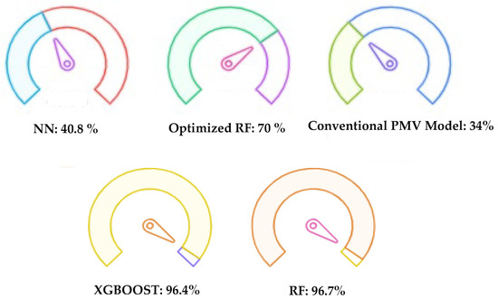
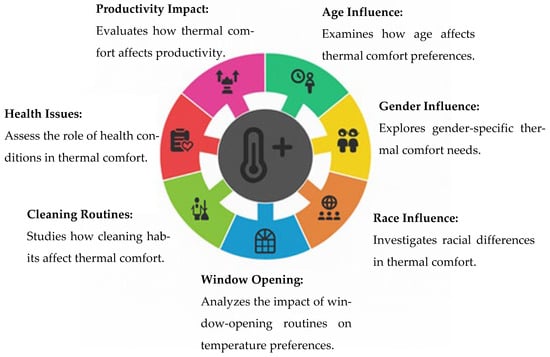
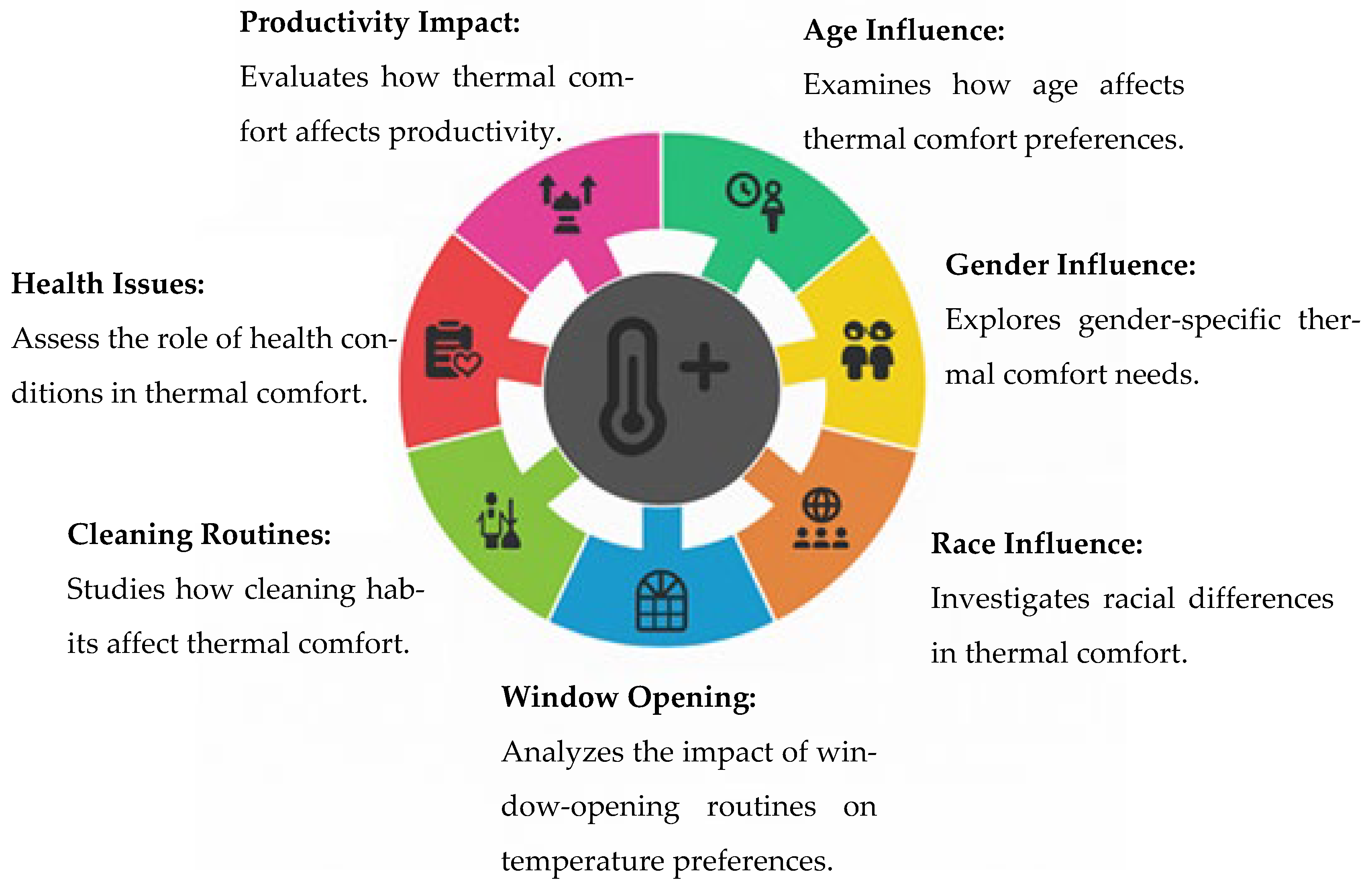
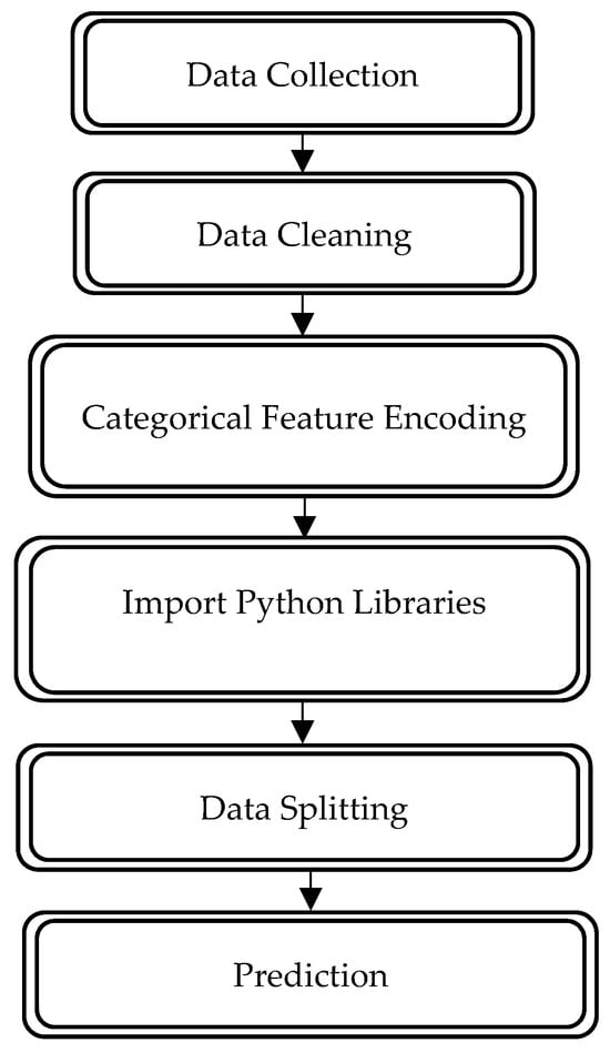
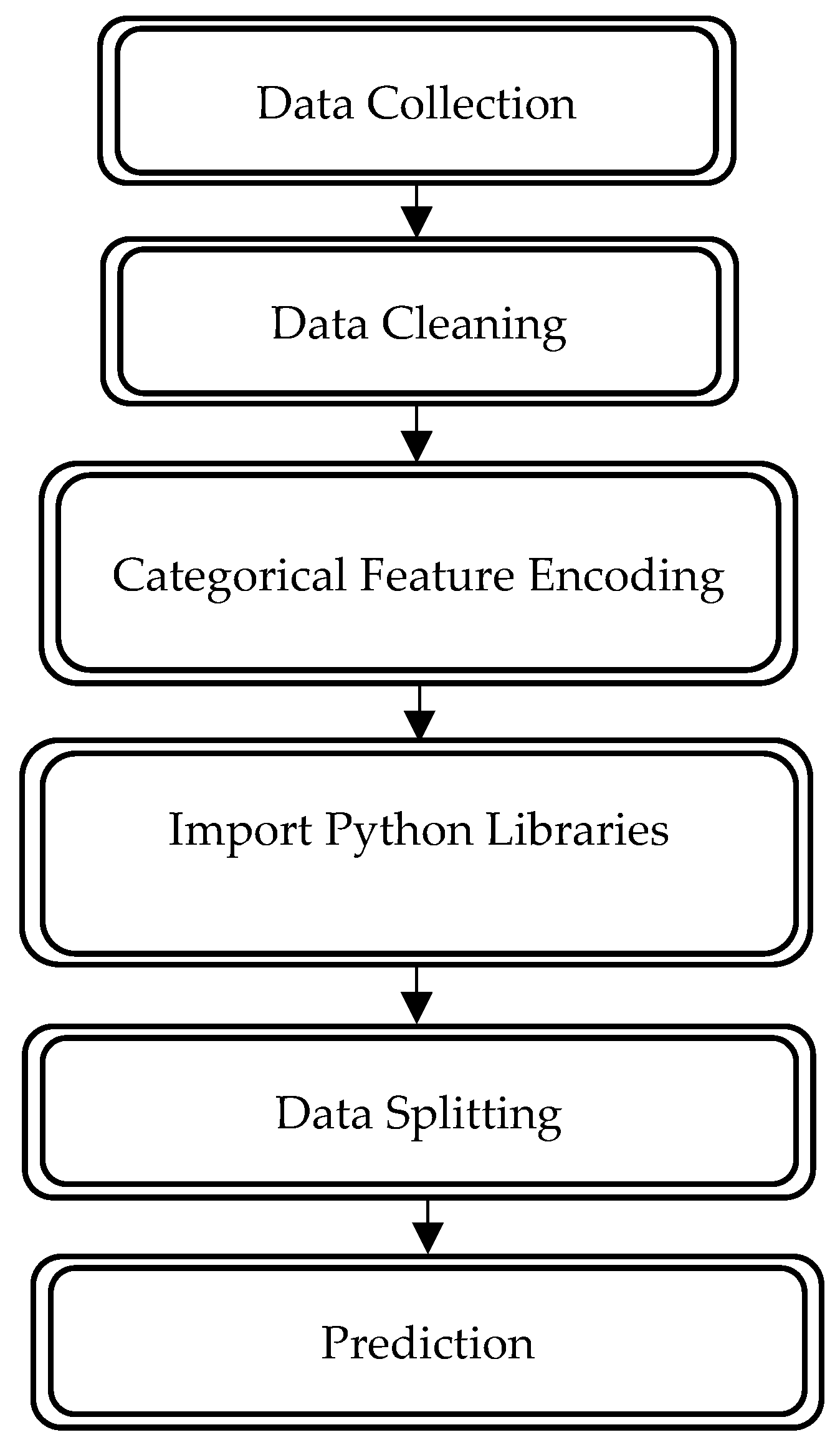
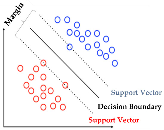
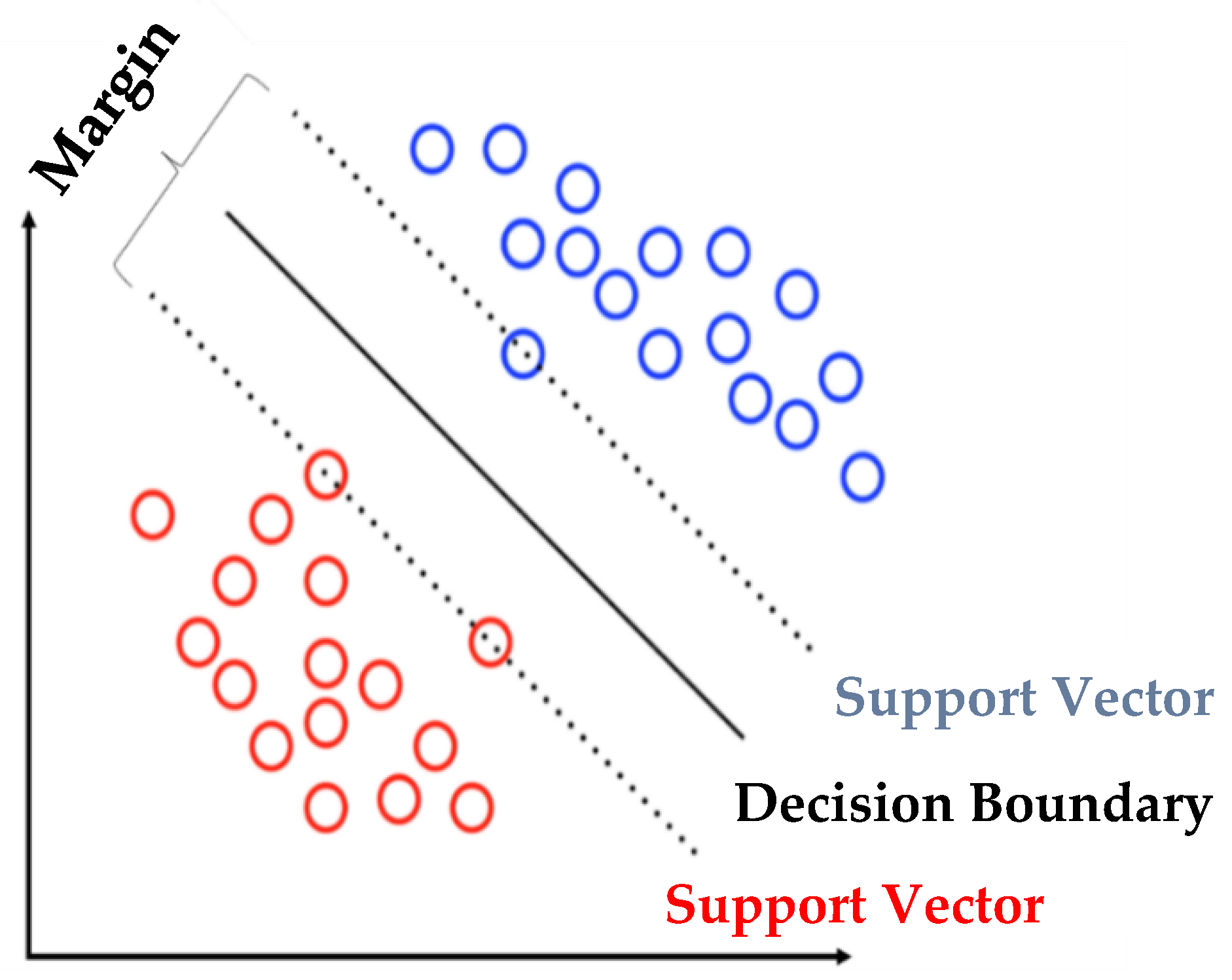
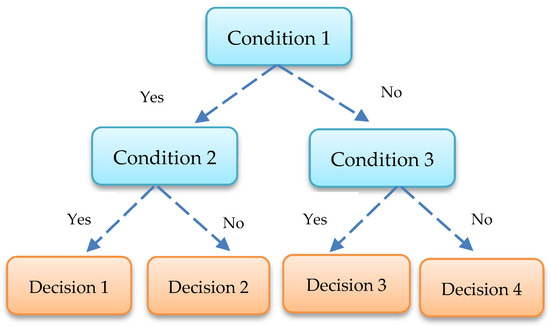
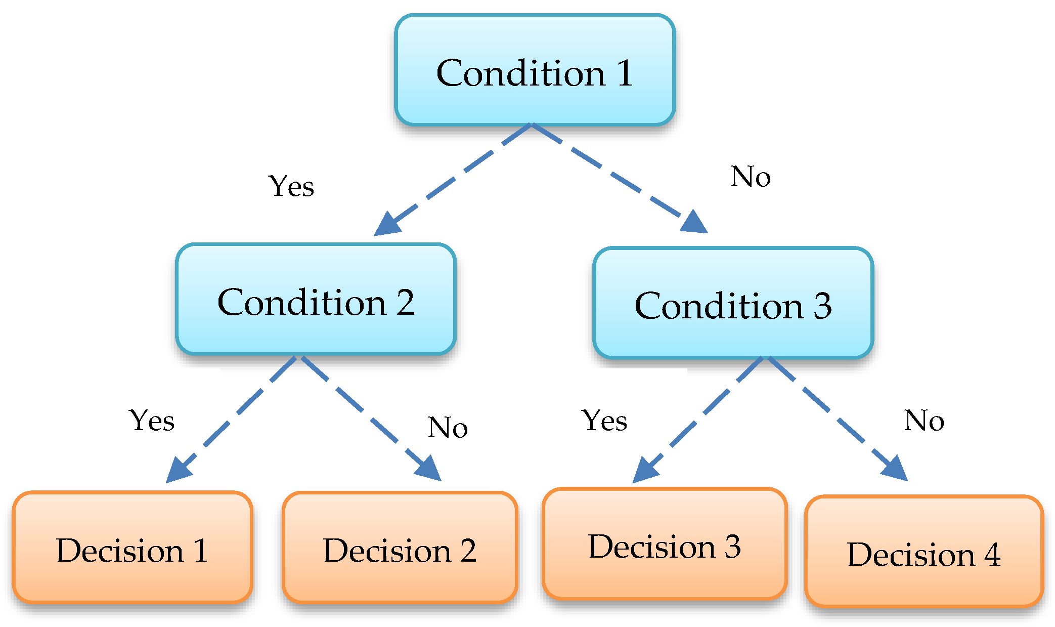
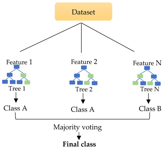
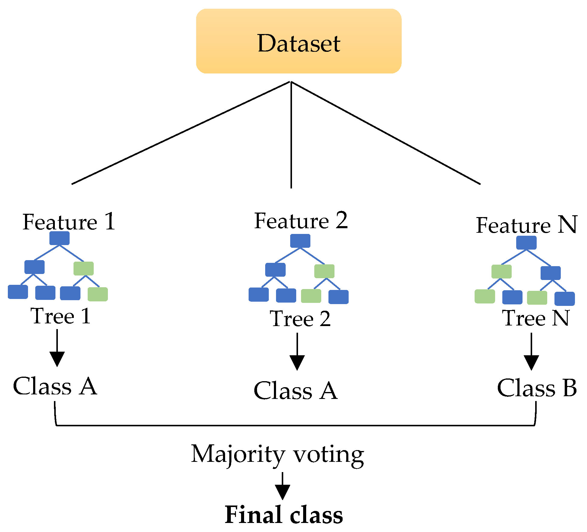
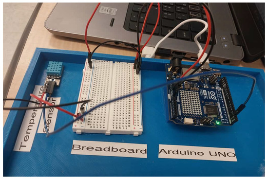
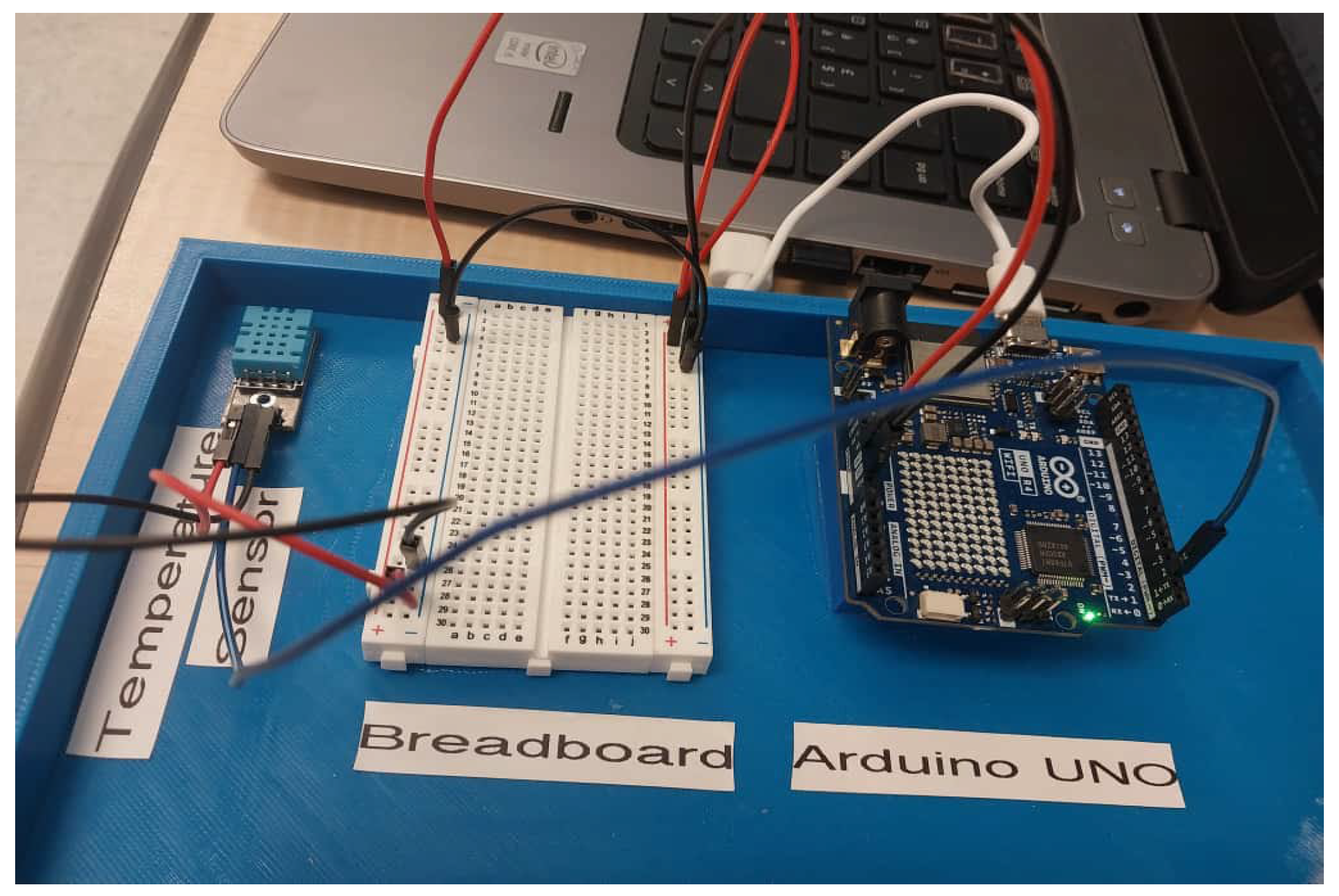
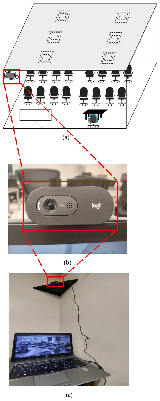
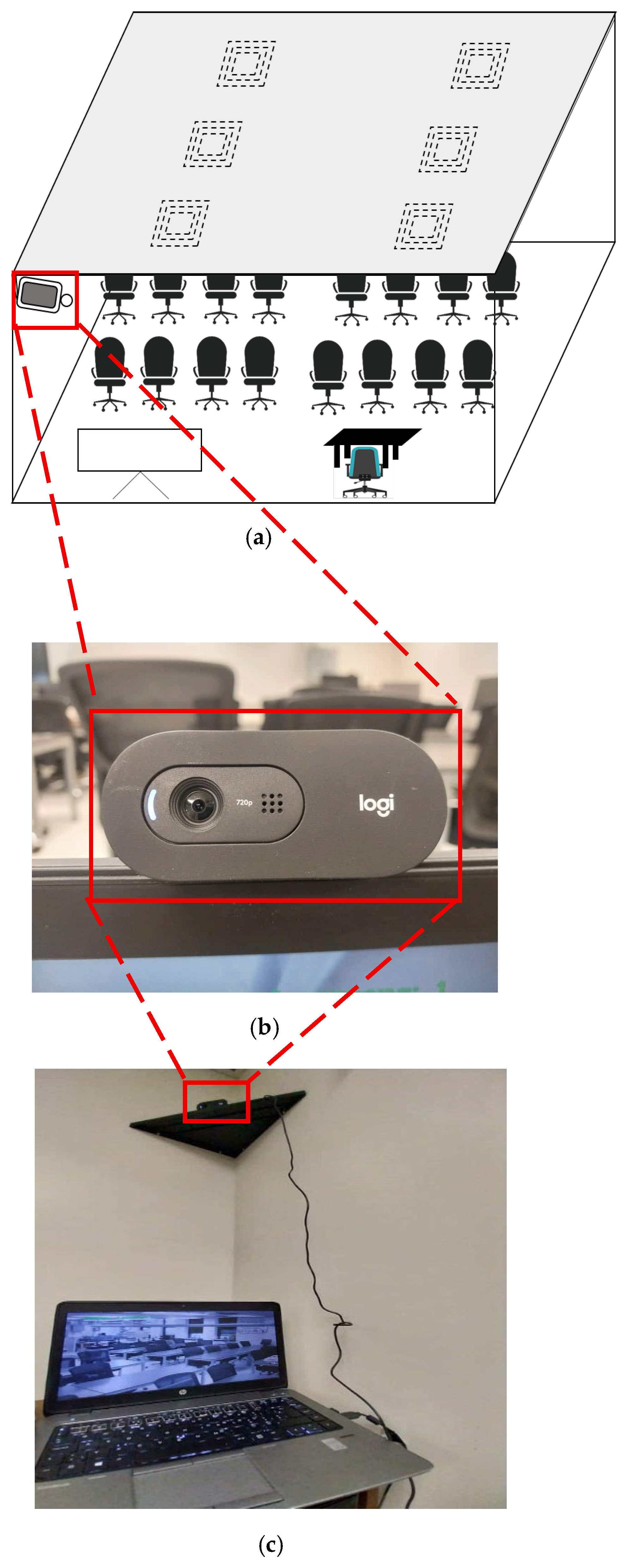
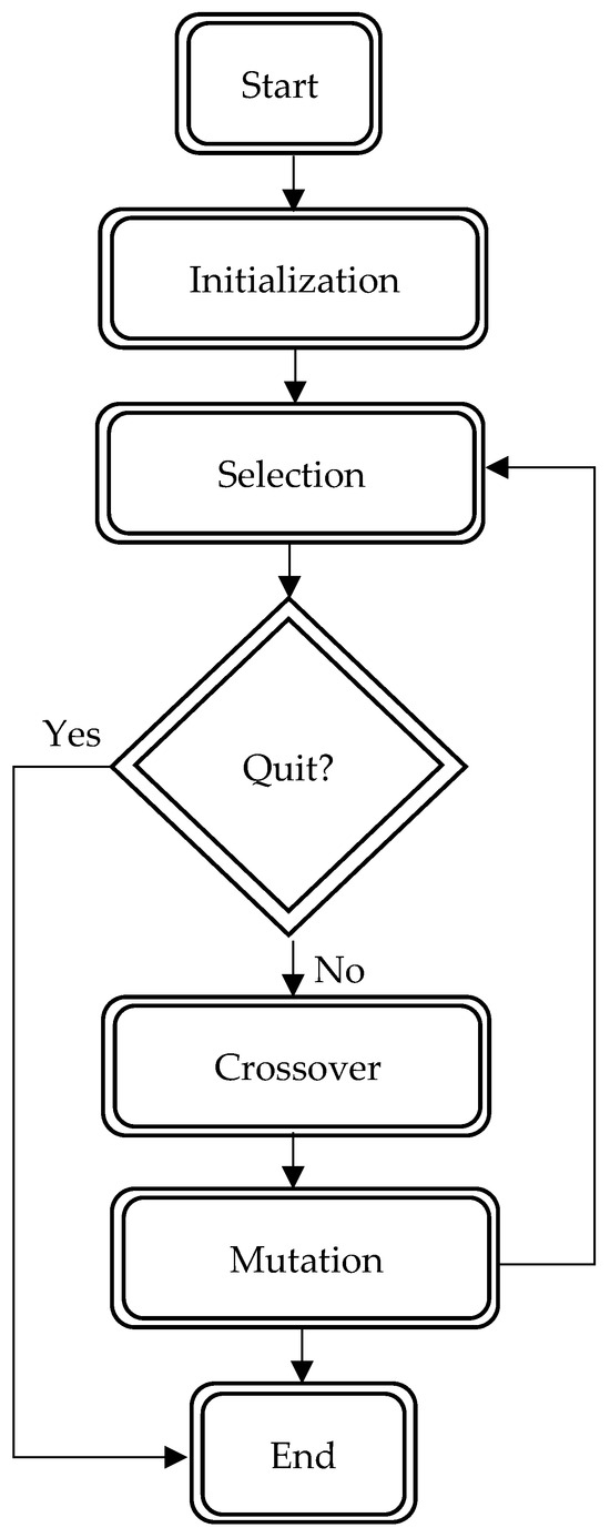
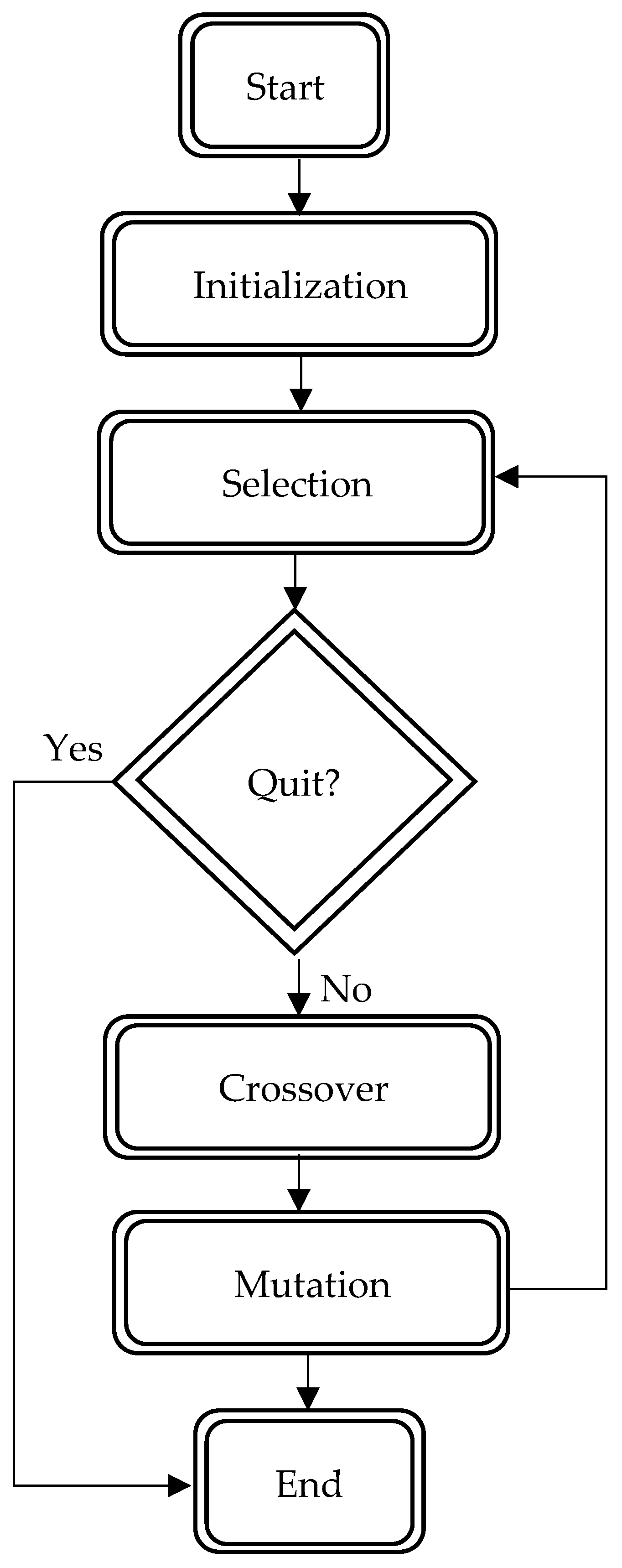
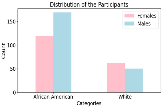
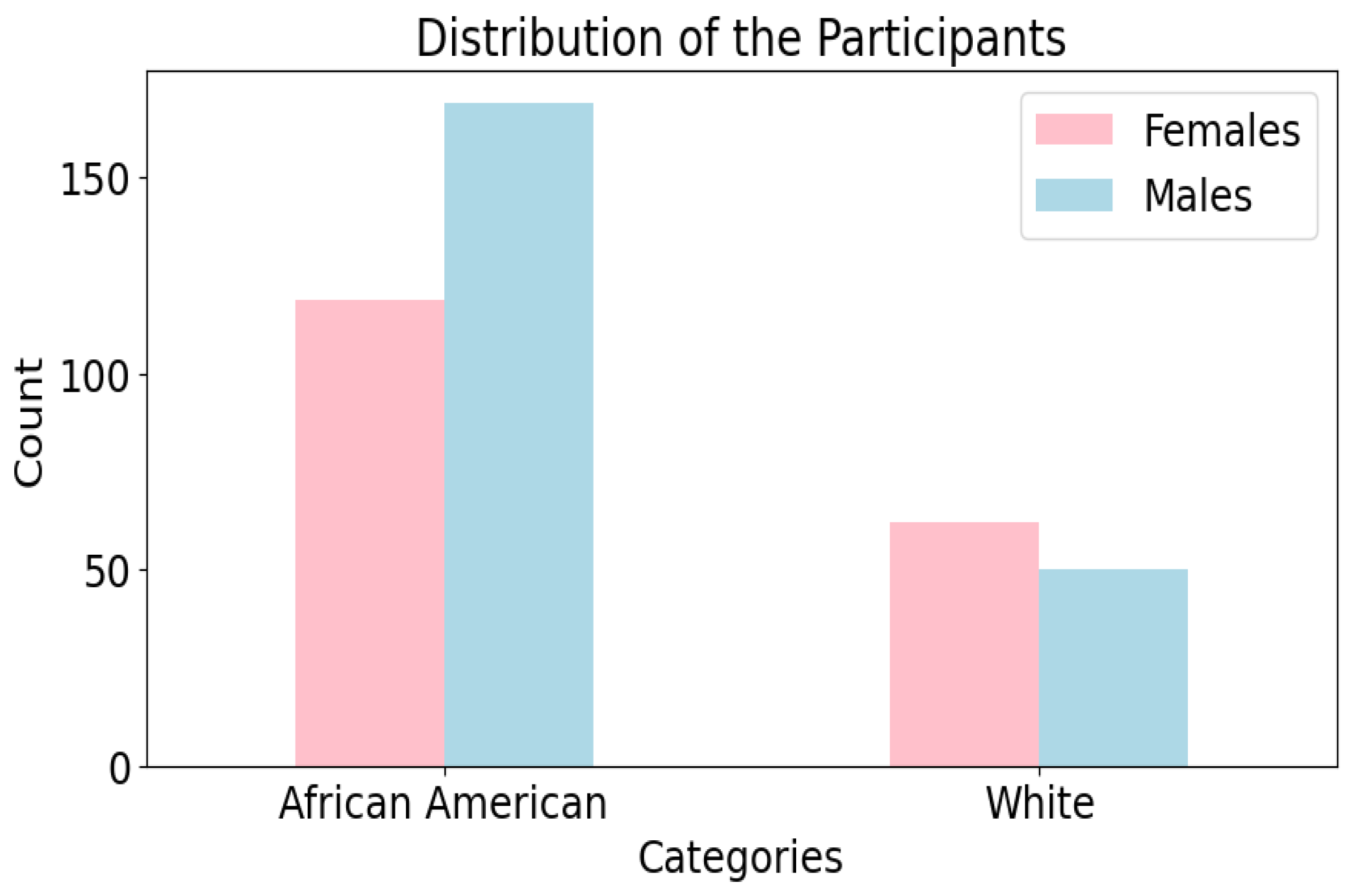
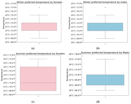
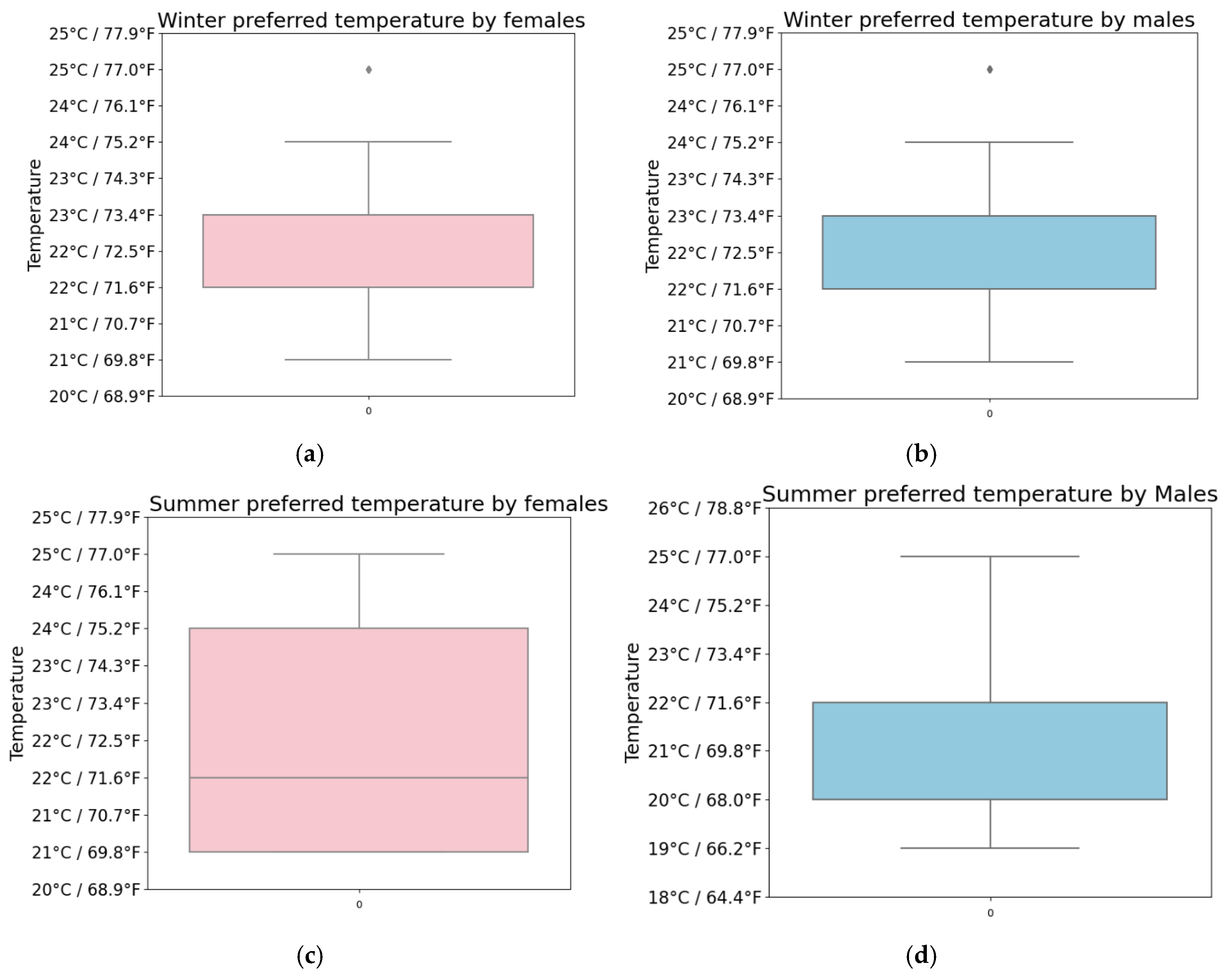
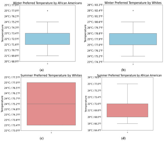
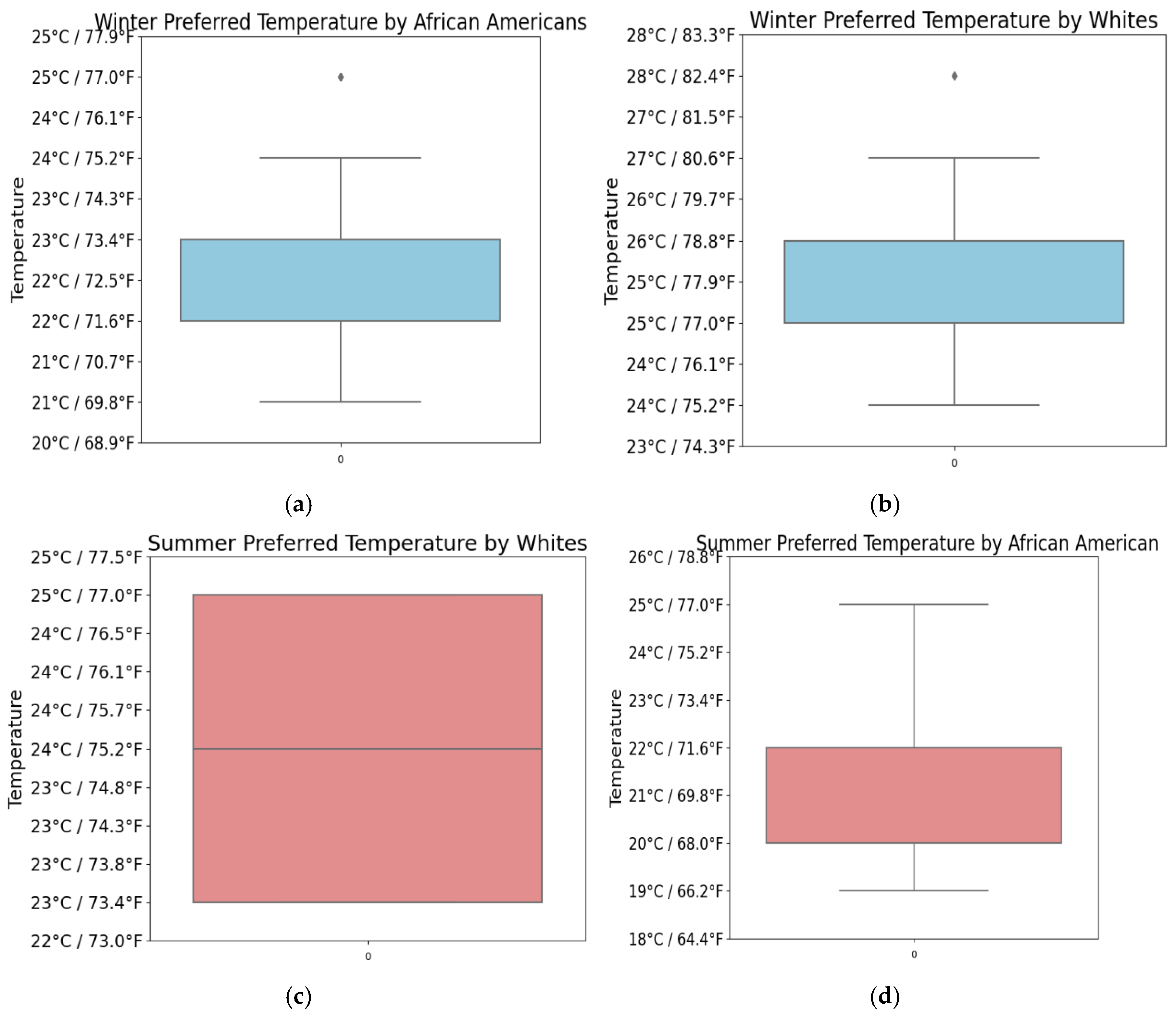
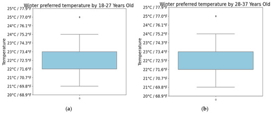
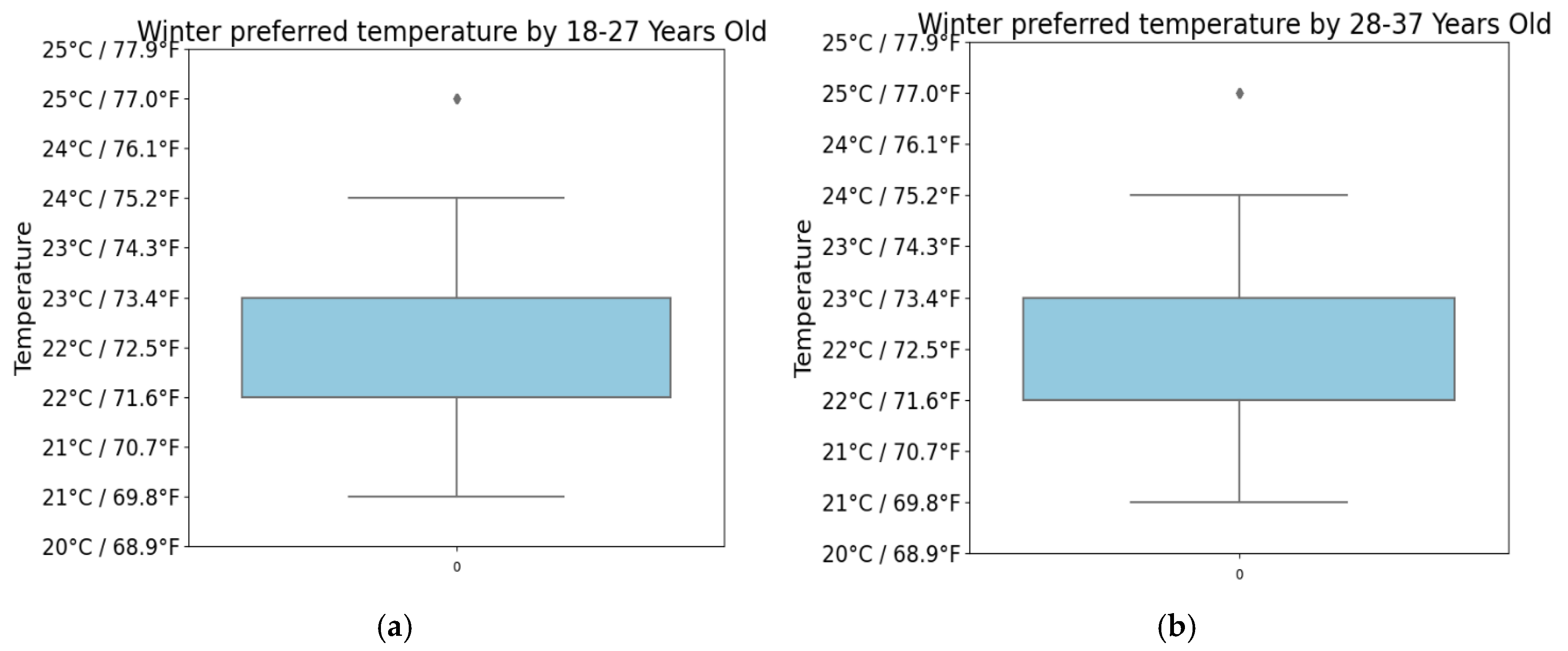
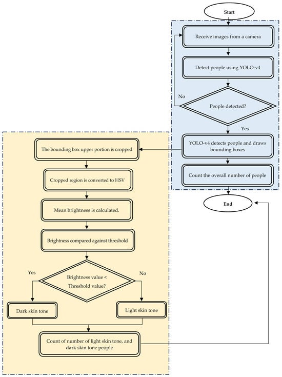
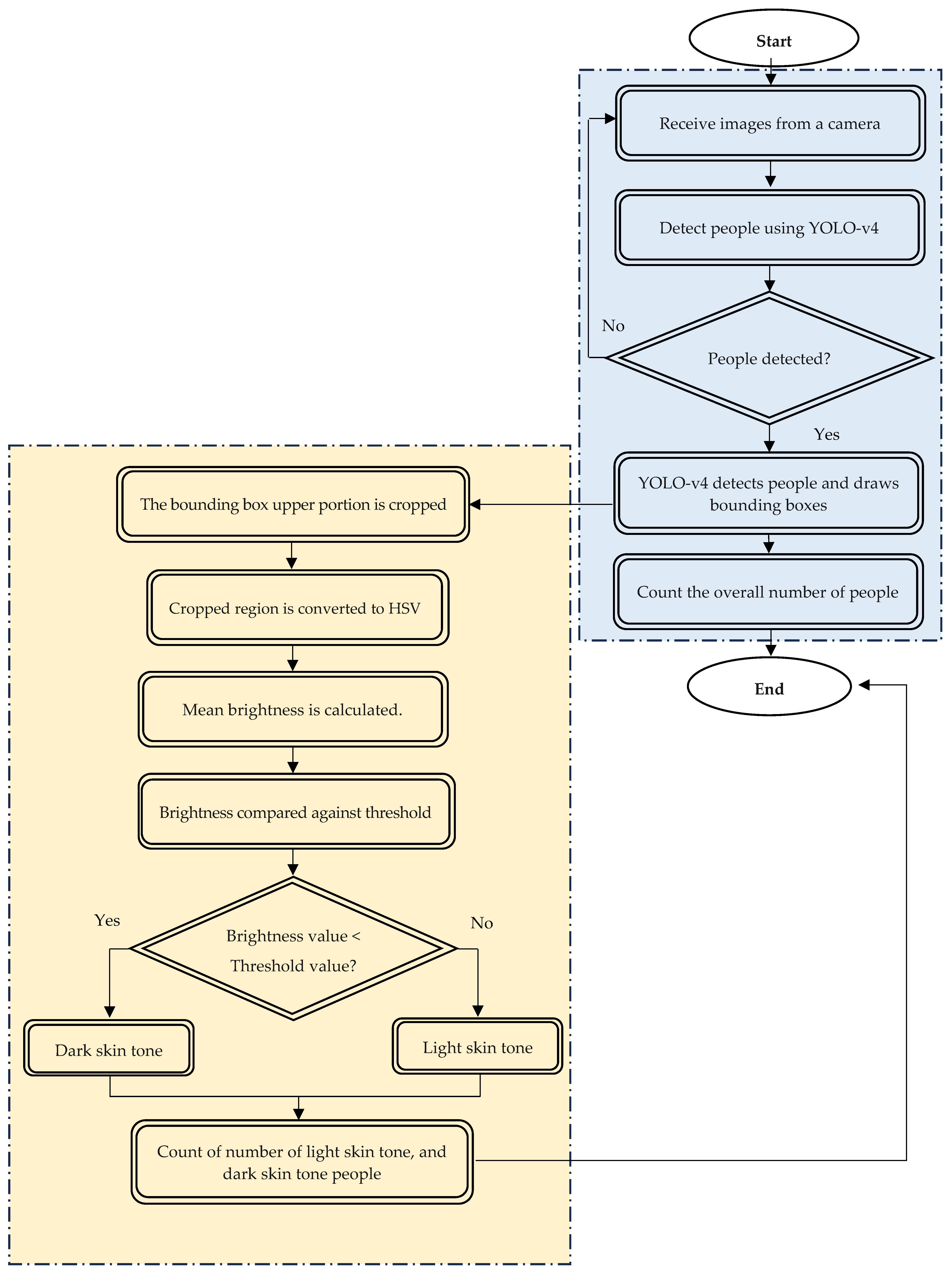
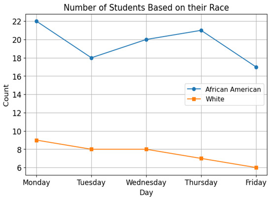

Disclaimer/Publisher’s Note: The statements, opinions and data contained in all publications are solely those of the individual author(s) and contributor(s) and not of MDPI and/or the editor(s). MDPI and/or the editor(s) disclaim responsibility for any injury to people or property resulting from any ideas, methods, instructions or products referred to in the content. |
© 2026 by the authors. Licensee MDPI, Basel, Switzerland. This article is an open access article distributed under the terms and conditions of the Creative Commons Attribution (CC BY) license.