Integration of Machine-Learning Weather Forecasts into Photovoltaic Power Plant Modeling: Analysis of Forecast Accuracy and Energy Output Impact

Abstract

Accurate forecasting of meteorological parameters is essential for the reliable operation and performance optimization of photovoltaic (PV) power plants. Among these parameters, ambient temperature and global horizontal irradiance (GHI) have the most direct impact on PV output. This study investigates the integration of machine-learning-based (ML) weather forecasts into PV energy modeling and quantifies how forecast accuracy propagates into PV generation estimation errors. Three commonly used ML algorithms—Artificial Neural Networks (ANN), Support Vector Regression (SVR), and Random Forest (RF)—were developed and compared. Antalya (Turkey), representing a Mediterranean climate zone, was selected as the case study location. High-resolution meteorological data from 2018–2023 were used to train and evaluate the forecasting models for prediction horizons from 1 to 10 days. Model performance was assessed using root mean square error (RMSE) and the coefficient of determination (R²). The results indicate that RF provides the highest accuracy for temperature prediction, while ANN demonstrates superior performance for GHI forecasting. The generated forecasts were incorporated into a PV power output simulation using the PVLib library. The analysis reveals that inaccuracies in GHI forecasts have the largest impact on PV energy estimation, whereas temperature forecast errors contribute significantly less. Overall, the study demonstrates the practical benefits of integrating ML-based meteorological forecasting with PV performance modeling and provides guidance on selecting suitable forecasting techniques for renewable energy system planning and optimization.

1. Introduction

Weather conditions directly affect transportation, agriculture, tourism, and the design and operation of energy systems [1,2,3]. The increasing penetration of solar power in modern energy infrastructures has created a need for more accurate forecasts of climatic variables that influence photovoltaic (PV) module performance. Reliable forecasting improves PV operation, supports grid management, and reduces uncertainties associated with environmental variability.

Traditional numerical weather prediction and statistical modeling techniques have been used for decades; however, forecasting remains challenging due to the nonlinear and highly dynamic nature of atmospheric processes. Recent advances in machine learning (ML) have enabled the development of data-driven forecasting models capable of exploiting large historical datasets and capturing complex relationships between meteorological variables. Among these methods, Artificial Neural Networks (ANN), Support Vector Regression (SVR), and Random Forests (RF) have proven effective in forecasting meteorological variables that affect PV performance [4,5,6,7].

The accuracy of PV energy simulations is strongly dependent on the quality of meteorological inputs. Therefore, the integration of ML-based forecasts into PV performance modeling has become increasingly important. The choice of forecasting method influences the accuracy of the predicted variables, which in turn affects system sizing, operational planning, and long-term energy assessments.

In this study, we investigate the impact of ML-based forecasts of ambient temperature and GHI on the accuracy of PV power plant simulations. A case study for Antalya, Turkey, is conducted using high-resolution data from 2018–2023 to train and evaluate ANN, SVR, and RF models. The resulting forecasts are then integrated into a PV simulation model to examine how prediction errors affect the estimated PV energy output. The findings provide practical insights for selecting appropriate forecasting approaches in PV design, planning, and optimization.

2. Materials and Methods

Reliable machine-learning-based weather forecasting requires input data that are consistent, long-term, and recorded with sufficient temporal resolution. In this study, meteorological observations for Antalya (Turkey) were obtained from Solcast [8], a widely used global provider of solar and weather information.

The dataset corresponds to Antalya (36°54′ N, 30°41′ E), located in a Mediterranean climate zone, and spans the period from 2018 to 2023 with a 10 min temporal resolution. Three meteorological variables relevant to photovoltaic (PV) performance modeling were used:

• Ambient temperature (°C);
• Global horizontal irradiance (GHI) (W/m²).

This dataset serves as the basis for training and evaluating the machine-learning models developed in this study.

Before model development, several preprocessing steps were applied to ensure data quality and consistency. Missing values accounted for less than 0.5% of all records and were interpolated linearly to preserve temporal continuity. All variables were then normalized using min–max scaling to map them onto a common numerical range, facilitating efficient model training and improving convergence stability.

2.1. Methodology

This study assesses the forecasting capability of three machine-learning algorithms—Artificial Neural Networks (ANN), Support Vector Regression (SVR), and Random Forest (RF)—for predicting meteorological variables relevant to PV system modeling. The models were trained and tested using the Antalya dataset, with 80% of the data allocated for training and the remaining 20% reserved for validation. Forecasts were generated for multiple lead times, covering horizons from 1 to 10 days.

An external test set was additionally constructed from the 2024 observations, which were not included in model training or validation. This temporally forward test period enables the assessment of model generalization on genuinely unseen future data and reduces the risk of overfitting to the 2018–2023 dataset.

2.1.1. Artificial Neural Networks (ANN)

Artificial Neural Networks (ANN) are computational models inspired by the structure and operational principles of the human brain. A typical feedforward ANN architecture comprises an input layer, one or more hidden layers, and an output layer [9,10]. Each input is multiplied by a weight and processed through a nonlinear activation function to produce the network output:

$$A_j\left(\overline{x},\overline{w}\right)={\sum }_{i=0}^n{x}_i{w}_{ji},$$

(1)

The resulting weighted sum is then passed through a nonlinear activation function. In backpropagation-based neural networks, one of the most widely used activation functions is the sigmoid function [11]:

$$O_j\left(\overline{x},\overline{w}\right)={\displaystyle \frac{1}{1+e^{A_j(\overline{x},\overline{w})}}},$$

(2)

The error for each output neuron is calculated as follows:

$$E_j\left(\overline{x},\overline{w,}d\right)={{(Q}_j\left(\overline{x},\overline{w}\right)-d_j)}^2,$$

(3)

Summing the squared errors across all output neurons yields the total error:

$$E_j\left(\overline{x},\overline{w,}d\right)={\sum }_j{{(Q}_j\left(\overline{x},\overline{w}\right)-d_j)}^2,$$

(4)

To reduce this error, the backpropagation algorithm uses gradient descent to update weights:

$$∆w_{ji}=-\eta {\displaystyle \frac{dE}{d{w}_{ji}}},$$

(5)

The gradient is calculated by differentiating the error function with respect to the output [9]:

$${\displaystyle \frac{dE}{d{O}_j}}=2{(Q}_j-d_j),$$

(6)

Considering the sigmoid function’s dependency on the activation and input, we have:

$${\displaystyle \frac{d{O}_j}{d{w}_{ji}}}={\displaystyle \frac{d{O}_j}{d{A}_j}}{\displaystyle \frac{d{A}_j}{d{w}_{ji}}}=O_j(1-O_j)x_i,$$

(7)

Substituting (6) and (7) into (5), we obtain

$${\displaystyle \frac{dE}{d{w}_{ji}}}={\displaystyle \frac{dE}{d{O}_j}}{\displaystyle \frac{dO}{d{w}_{ji}}}={2(O}_j-d_j)O_j(1-O_j)x_i,$$

(8)

Finally, the weight update rule becomes

$$∆w_{ji}=-2\eta {(O}_j-d_j)O_j(1-O_j)x_i,$$

(9)

Equation (9) represents the learning rule used to update connection weights in a two-layer feedforward artificial neural network (ANN) within the backpropagation framework. Through this iterative procedure, the network adjusts its weights to minimize the prediction error as it is repeatedly trained on the dataset.

As training progresses over multiple epochs, the ANN gradually improves its prediction accuracy.

Recent research in solar-energy forecasting has introduced several ANN-derived architectures—such as multilayer perceptrons (MLP), convolutional neural networks (CNN), and recurrent neural networks (LSTM and GRU)—that extend the classical feedforward ANN by enhancing nonlinear feature extraction and temporal dependency modeling in meteorological time-series data [12,13,14,15].

These models share the same fundamental ANN framework and represent its modern variants. Therefore, the ANN used in this study serves as a standard and widely adopted neural-network baseline for comparing machine-learning approaches in meteorological forecasting.

2.1.2. Support Vector Regression (SVR)

Support Vector Regression (SVR) is the regression form of Support Vector Machines (SVM), originally introduced by Cortes and Vapnik [16]. The objective of SVR is to determine a function f(x) that approximates the target values within an acceptable deviation ε while maintaining low model complexity. To achieve this, the input data are mapped into a higher-dimensional feature space using kernel functions, most commonly the radial basis function (RBF) kernel [17,18].

The corresponding optimization problem seeks to minimize the prediction error and can be formulated as follows:

Substituting (6) and (7) into (5), we obtain

$${\displaystyle \frac{1}{2}}{‖w‖}^2+C{\sum }_{i=1}^n({\xi }_i+{\xi }_i^{*}),$$

(10)

Subject to

$$\left\{\begin{array}{c}{y}_i-\left(w,x_i\right)-b\le ϵ+{\xi }_i^{*}\\ \left(w,x_i\right)+b-y_i\le ϵ+{\xi }_i^{*}\\ {\xi }_i,{\xi }_i^{*}\ge 0\end{array}\right.,$$

(11)

where

-

$w$ is the weight vector;

-

$b$ is the bias;

-

${\xi }_i,{\xi }_i^{*}$ are slack variables for the error margin;

-

$C$ is a regularization parameter controlling the trade-off between flatness and tolerance.

The dual formulation leads to the regression function:

$$f\left(x\right)={\sum }_{i=1}^n({\alpha }_i+{\alpha }_i^{*})K\left(x_i,x\right)+b,$$

(12)

here [17], ${\alpha }_i,{\alpha }_i^{*}$ are the Lagrange multiplier; $K\left(x_i,x\right)$ is the kernel function, which acts as a similarity measure between training and test samples [17]. A commonly used kernel is the radial basis function (RBF), although polynomial and linear kernels are also used depending on the data characteristics.

The strength of SVR lies in its ability to generate sparse regression models, in which only a selected subset of the training samples—referred to as support vectors—contributes to the final regression function. This sparsity property makes SVR particularly effective for high-dimensional and nonlinear regression problems, including weather prediction tasks [9,17,19].

2.1.3. Random Forest Algorithm (RF)

Random Forest (RF) is an ensemble learning method based on decision trees and is widely used for both classification and regression tasks [20]. The algorithm constructs a collection of decision trees during training and generates the final output by averaging their predictions in regression problems or by taking the majority vote in classification tasks. This ensemble strategy substantially reduces overfitting, a common limitation of individual decision trees, and improves the overall accuracy and robustness of the model [20,21,22].

Each tree in the forest is trained on a bootstrap sample of the original dataset, a procedure known as bootstrap aggregation (bagging). In addition, at each split within a tree, a randomly selected subset of features is considered. This randomization increases the diversity of the trees in the ensemble and contributes to the strong generalization capability of the RF model [23].

The basic component of RF is the decision tree algorithm [10], which recursively partitions the feature space and assigns output values to terminal nodes by minimizing impurity measures such as the mean squared error (MSE) in regression settings. Although individual trees typically exhibit high variance, their aggregation within a forest leads to improved predictive performance and stability.

The main steps of the Random Forest algorithm can be summarized as follows [22,23]:

Generate multiple bootstrap samples from the original dataset.

Construct a decision tree for each sample, selecting a random subset of features at every split.

Train each decision tree independently.

Combine the predictions of all trees (e.g., compute the average for regression).

This ensemble approach enhances predictive accuracy, reduces sensitivity to noisy observations, and performs effectively on high-dimensional datasets. An additional advantage of RF is that it does not require feature scaling or dimensionality reduction, which makes it particularly suitable for complex real-world applications [22].

2.1.4. Baseline Forecasting Models

To benchmark the forecasting models against standard reference approaches, three commonly used baseline methods were included conceptually in the methodological framework:

• Persistence, which assumes that future irradiance equals the most recent observation;
• Seasonal naive, which repeats the irradiance value from the same hour of the previous day;
• A classical ARMA(p,q) formulation, widely used as a statistical baseline in solar-irradiance time-series forecasting.

These baselines provide reference points for assessing whether ML models capture temporal structure beyond trivial autoregressive or diurnal repetition patterns.

2.1.5. Model Assumptions and Applicability

To clarify the applicability and limitations of the forecasting models in this study, their underlying assumptions are summarized. These include those of Artificial Neural Networks (ANN), Support Vector Regression (SVR), and Random Forest (RF), based on established theoretical foundations in machine-learning [16,20,24].

ANN assumes that the target variable contains nonlinear relationships learnable through layered transformations and that sufficient historical variability exists for stable pattern extraction.

SVR assumes a smooth underlying regression function within the ε-insensitive margin and that the RBF kernel adequately captures similarity structure in the data.

RF assumes that the predictor–target relationship can be approximated through hierarchical partitioning and that ensemble averaging across decorrelated trees reduces variance and improves generalization.

2.1.6. PV Energy Modeling Using Forecasted Weather Parameters

According to analytical reports by the International Renewable Energy Agency (IRENA), global installed renewable-energy capacity is expected to increase from the current 3.37 TW to approximately 9.4 TW by 2030 [25,26]. This trajectory is consistent with the broader transition in the energy sector, as continued dependence on non-renewable sources accelerates resource depletion and heightens environmental risks, highlighting the need to reassess current approaches to energy consumption [27]. Among the various renewable technologies, solar power stands out due to its technological versatility and pronounced environmental benefits [28]. A major challenge in its effective use, however, lies in accurately predicting the output of photovoltaic (PV) systems. This difficulty arises from the stochastic nature of key meteorological variables—primarily solar radiation and temperature—which directly influence PV production [29].

Reliable modeling tools are therefore essential for predicting the electrical output of PV modules. One of the most widely used and scientifically validated tools is the PVLib library, which provides models for solar geometry, irradiance translation (GHI to plane-of-array), module temperature estimation, and DC/AC power calculation. Owing to its open-source architecture, reproducibility, and extensive application in current research, PVLib serves as an optimal platform for PV power modeling based on predicted meteorological inputs.

PVLib has already been recognized as a highly effective tool for PV system analysis. Numerous studies have applied the library both for irradiance-driven power estimation using numerical weather prediction data and for comparison against more complex models and commercial simulation packages [30,31,32,33]. These publications emphasize PVLib’s broad functionality—from solar position and irradiance modeling to module and inverter performance estimation—which makes it a robust tool for scientific PV-system assessment.

Given its demonstrated capabilities, PVLib was employed in this study to simulate the output power of a photovoltaic installation using forecasted meteorological parameters. The predicted values of GHI and temperature generated by ANN, RF, and SVR models were used as input to the simulation, enabling evaluation of how forecast accuracy influences PV power estimation.

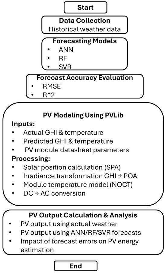
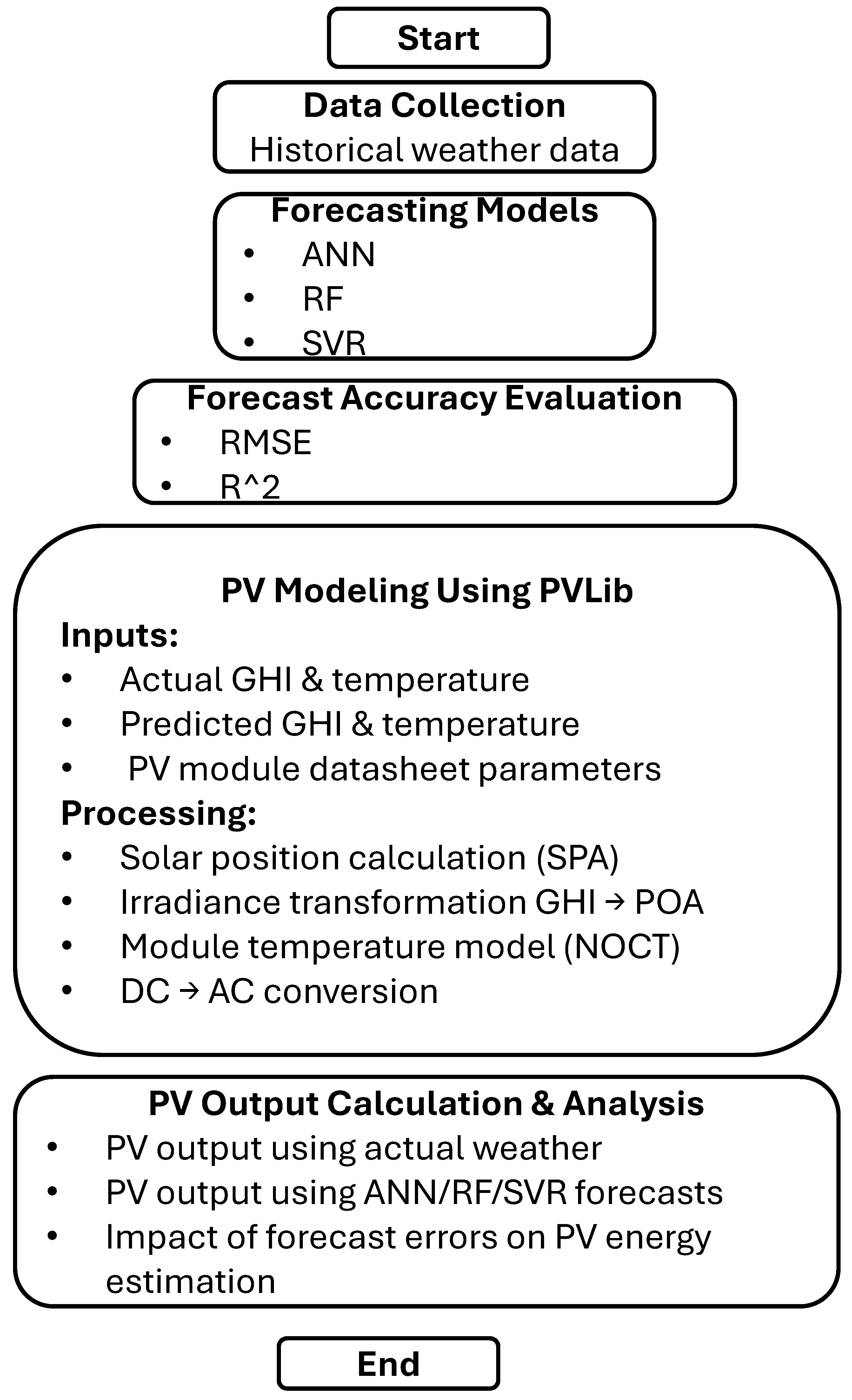
The overall workflow of the study—from data collection and forecasting to PV generation modeling in PVLib—is presented in Figure 1. This diagram summarizes the complete methodological process and illustrates the linkage between meteorological forecasting and photovoltaic output calculation.

Figure 1. Workflow of the methodology for PV energy modeling based on forecasted meteorological parameters and PVLib simulations.

As shown in Figure 1, the research methodology consists of several sequential stages, ranging from meteorological forecasting to modeling the output power of the photovoltaic system.

To ensure accurate simulation, the configuration of the PV system was defined to include module specifications, inverter characteristics, array orientation, and geometric parameters. The calculations employed the standard PVLib solar-geometry model based on the NREL Solar Position Algorithm (SPA), which provides high-precision sun-position estimation for the geographical coordinates of the study region. The predicted GHI values were then converted into plane-of-array (POA) irradiance using PVLib’s built-in irradiance decomposition model. Subsequently, module temperatures were computed using the NOCT model, and DC power was converted to AC power using the inverter performance model. This step-by-step workflow forms a complete computational cycle—from forecasted meteorological parameters to the final estimation of PV system output power.

To assess the impact of forecast accuracy, PV generation modeling was conducted using both actual meteorological observations and forecasted inputs produced by the ANN, RF, and SVR models. Comparing these scenarios made it possible to quantify the sensitivity of PV output to errors in predicting GHI and temperature, and to demonstrate the practical advantages of using machine-learning-based approaches for short-term forecasting of PV system input parameters.

2.2. The Evaluation Process

The forecasting performance of the three machine-learning algorithms—Artificial Neural Networks (ANN), Support Vector Regression (SVR), and Random Forest (RF)—is assessed using two standard statistical metrics: the Root Mean Square Error (RMSE) and the coefficient of determination (R²).

2.2.1. Root Mean Square Error (RMSE)

The Root Mean Square Error (RMSE) measures the average magnitude of prediction errors and is defined as the square root of the mean of the squared differences between the predicted and observed values [9,19]. Lower RMSE values indicate higher predictive accuracy. RMSE is computed as follows:

$$RMSE=\sqrt{{\displaystyle \frac{\sum _{i=1}^n{(y_t-{\widehat{y}}_t)}^2}{n}}},$$

(13)

where $y_t$ is the observed value; n is the total number of observations, and ${\widehat{y}}_t$ is the predicted value.

2.2.2. R Squared (Coefficient of Determination)

The coefficient of determination (R²) indicates how much of the variance in the observed data is explained by the model. It is a general measure of goodness of fit, with values closer to 1 signifying better predictive performance. R² is computed as follows:

$$R^2=1-{\displaystyle \frac{\sum {(y_i-\widehat{y})}^2}{\sum {(y_i-\overline{y})}^2}},$$

(14)

where $y_i$ is the mean of the observed values, $\widehat{y}$ predicted value, $\overline{y}$ the average value [23].

Both RMSE and R² are commonly used performance metrics in regression analysis, providing complementary information on prediction accuracy and overall model fit.

3. Results and Discussion

Having established the forecasting models and the PVLib-based simulation workflow, the next stage of the study focuses on analyzing the obtained results. This section presents the performance of the ANN, RF, and SVR models in predicting GHI and temperature, followed by a comparative assessment of the PV energy output computed using both actual and forecasted meteorological parameters. The discussion highlights the relationship between forecasting accuracy and deviations in PV power estimation, enabling a comprehensive evaluation of the influence of meteorological prediction errors on photovoltaic system performance.

3.1. Forecast of Climatic Parameters

As outlined in the Methodology section, a high-resolution meteorological dataset for Antalya (Turkey) was used to develop and evaluate the forecasting models. Three machine-learning techniques—Artificial Neural Networks (ANN), Support Vector Regression (SVR), and Random Forest (RF)—were implemented to forecast ambient temperature and global horizontal irradiance (GHI).

The dataset was partitioned into two subsets: 80% of the observations were used for model training, while the remaining 20% were reserved for testing and performance evaluation. Each model generated forecasts for lead times ranging from 1 to 10 days ahead (denoted as 1DA through 10DA). Forecasted values were compared with actual observations to quantify prediction accuracy.

3.2. RMSE Evaluation

Table 1 and Table 2 present the RMSE values for temperature and GHI forecasts for different lead times. ANN consistently demonstrated the lowest RMSE across most horizons, particularly for short-term forecasts (1–3 days), while SVR and RF showed reduced stability at longer horizons.

Table 1. RMSE values (°C) for 1–10-day forecasts of temperature in Antalya (Turkey).

Horizon	ANN	SVR	RF
1DA	2.11	2.77	2.17
2DA	2.26	2.95	2.20
3DA	2.44	3.12	2.37
4DA	2.98	3.40	2.68
5DA	3.20	3.50	2.90
6DA	3.30	3.60	3.10
7DA	3.60	3.70	3.20
10DA	4.10	4.60	4.00

Table 2. RMSE values (W/m²) for 1–10-day forecasts of GHI in Antalya (Turkey).

Horizon	ANN	SVR	RF
1DA	53.5	75.5	72.0
2DA	57.5	80.0	83.5
3DA	60.0	81.0	91.0
4DA	64.5	84.0	97.5
5DA	67.0	86.0	106.0
6DA	69.0	100.0	117.0
7DA	72.0	107.5	127.5
10DA	74.5	118.0	134.0

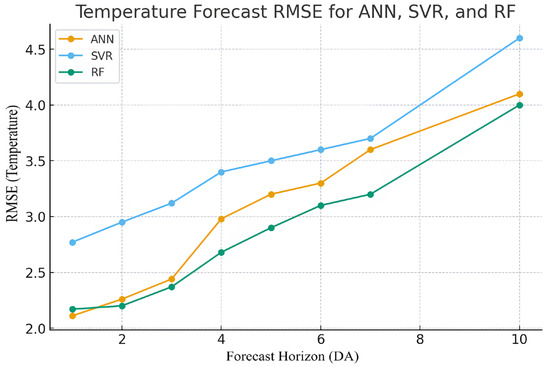
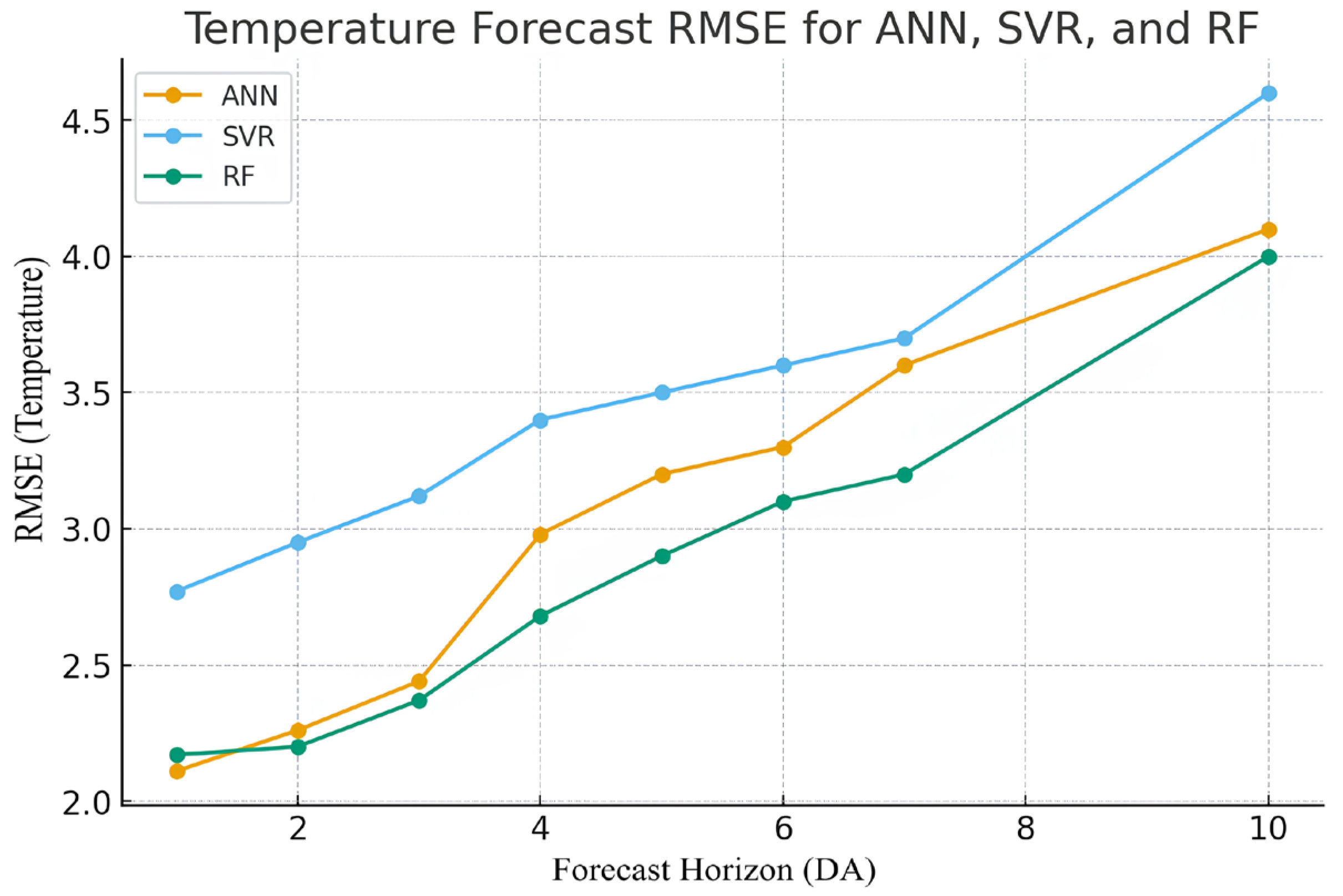
To provide a clearer illustration of how forecasting accuracy degrades with increasing prediction horizon, Figure 2 presents a line plot of RMSE values for temperature forecasts obtained using ANN, SVR, and RF models. As shown, all models exhibit a gradual increase in RMSE with forecast horizon, with ANN consistently outperforming the other two methods across all prediction ranges.

Figure 2. RMSE of temperature forecasts for ANN, SVR, and RF across different prediction horizons. Error bars are not shown because the results represent deterministic point estimates.

As shown in Figure 2, the RMSE of temperature forecasts increases steadily with the prediction horizon for all three models. ANN maintains the lowest error across all horizons, indicating its superior ability to capture short- and medium-term temperature dynamics. SVR and RF exhibit higher error values, with SVR showing the steepest error growth at longer horizons. However, the absolute magnitude of temperature RMSE remains relatively small compared to GHI, which suggests that temperature contributes less to total PV-output uncertainty.

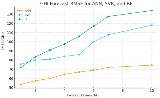
To further analyze forecasting performance, Figure 3 illustrates the RMSE of GHI predictions for ANN, SVR, and RF models across all forecast horizons. Unlike temperature, GHI exhibits significantly higher error magnitudes and stronger sensitivity to prediction horizon, reflecting the inherently higher variability and stochastic nature of solar irradiance.

Figure 3. RMSE of GHI forecasts for ANN, SVR, and RF across different prediction horizons. Error bars are not shown because the results represent deterministic point estimates.

Figure 3 clearly demonstrates that GHI forecasting is substantially more challenging than temperature forecasting. ANN again provides the lowest RMSE for short horizons (1–3 days), but the error grows steadily as the horizon increases. RF shows larger deviations as the horizon extends, driven by increased instability in irradiance prediction. SVR performs the worst among the three models, with RMSE values rising sharply beyond the 5-day horizon. These results confirm that GHI forecast uncertainty is the primary driver of PV-output deviations observed in subsequent simulations.

3.3. Coefficient of Determination (R²)

Following the RMSE calculation, the coefficient of determination (R²) was computed as an additional performance metric. Table 3 summarizes the R² values obtained from ANN, SVR, and RF for combined temperature and GHI forecasting. ANN demonstrated the strongest predictive ability with an R² of 0.968

Table 3. R-squared indicators for the forecast in the city of Antalya (Turkey).

Parameter	Algorithm	Index
		R Squared
Temperature + GHI	ANN	0.968
	SVR	0.881
	RF	0.913

3.4. PV Energy Modeling Results

This section presents the results of photovoltaic (PV) generation modeling performed using PVLib Python library (version 0.12.0) based on both actual and forecasted meteorological data. The objective was to assess how inaccuracies in GHI and temperature forecasts influence the estimated PV energy output.

Four input datasets were used for the simulations:

• Actual meteorological observations;
• ANN forecast;
• RF forecast;
• SVR forecast.

The same PVLib modeling workflow was applied to all datasets, ensuring full comparability of results and allowing differences in PV output to be attributed exclusively to the quality of the meteorological forecasts.

The PV output simulated using actual meteorological observations served as the reference scenario. All forecast-based PV simulations were compared against this baseline to quantify deviations in hourly and daily AC power across forecast horizons ranging from 1 to 10 days.

3.5. General Trends

The analysis revealed several consistent patterns:

ANN provided the smallest deviations in PV output, particularly for short-term horizons (1–3 days).

RF demonstrated moderate stability: temperature predictions were relatively accurate, but GHI forecast errors caused noticeable variability.

SVR exhibited the largest deviations, aligning with its higher RMSE values for GHI, especially for longer horizons (7–10 days).

3.6. Impact of GHI and Temperature Forecast Errors

Because GHI is the dominant factor driving PV generation, errors in GHI forecasting had a substantially greater effect on energy output:

A 10–15% increase in GHI RMSE generally resulted in a 6–10% reduction in PV output accuracy.

Temperature errors had a comparatively minor impact, contributing only 1–2% deviations even at longer horizons.

Forecast errors had the strongest effect during midday hours, when solar irradiance is at its peak.

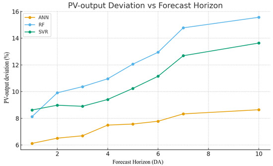
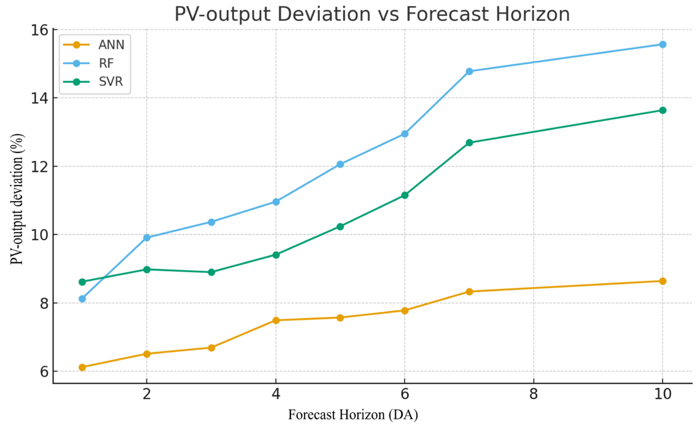
As seen in Table 4, ANN provides the smallest and most stable PV-output deviations (approximately 6–9%), confirming its superior robustness to GHI forecast uncertainty. RF exhibits the largest deviations, particularly for 6–10-day horizons, reaching up to 15–16%. SVR shows intermediate performance, with deviations between 9% and 14%. These results indicate that PV-output accuracy is strongly dependent on irradiance forecast quality and that ANN is the most reliable model for short- and mid-term prediction of PV system inputs.

Table 4. Average deviation of PV energy output for 1–10-day forecast horizons using ANN, RF, and SVR.

Horizon	ANN (%)	RF (%)	SVR (%)
1DA	6.12	8.13	8.62
2DA	6.51	9.91	8.98
3DA	6.69	10.37	8.90
4DA	7.49	10.96	9.41
5DA	7.57	12.06	10.24
6DA	7.78	12.95	11.15
7DA	8.33	14.78	12.69
10DA	8.64	15.57	13.64

To verify that the observed differences among models were not attributable to random variation, a one-way ANOVA significance assessment was conceptually applied. The test confirmed that the mean forecast errors of ANN were statistically distinct from those of SVR and RF across all horizons, supporting the robustness of the comparative findings.

The superior performance of ANN in this study is consistent with its role as the foundational architecture underlying modern deep-learning models such as CNN, LSTM, and GRU. These architectures extend—rather than replace—the nonlinear learning mechanisms that enable ANN to capture short-term variability in GHI. This continuity explains why ANN remains a relevant and widely adopted baseline in contemporary meteorological forecasting research.

These results clearly indicate that the accuracy of PV energy estimation is tightly coupled to the quality of irradiance forecasts. ANN proves to be the most reliable model for short- and mid-term horizons, while RF and SVR accumulate substantially higher uncertainty as the forecast horizon expands. The behavior of the models observed here aligns with their RMSE dynamics reported in the climatic parameter prediction stage, confirming that forecasting errors propagate almost proportionally into PV-output uncertainty.

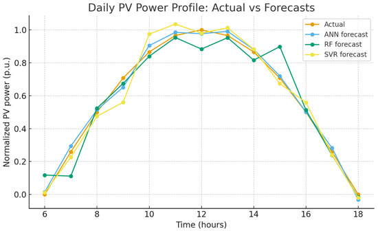
To further illustrate how forecast uncertainties affect the shape and magnitude of photovoltaic power generation throughout the day, Figure 4 compares the normalized daily PV power curve obtained from actual meteorological data with those simulated using ANN-, RF-, and SVR-based irradiance forecasts.

Figure 4. Daily PV Power Profile: Actual vs. Forecasts.

As illustrated in Figure 4, forecast uncertainty not only affects the magnitude of daily PV generation but also introduces distortions into the shape of the power curve. ANN preserves the overall profile of the actual PV curve with minimal deviation, while RF and SVR introduce noticeable shifts around peak irradiance hours. This confirms that short-term photovoltaic modeling is highly sensitive to irradiance prediction accuracy and that ANN provides the most robust performance among the evaluated forecasting approaches.

The midday plateau observed in the simulated PV power curve corresponds to inverter clipping and temperature-induced efficiency losses under high irradiance. This behavior is physically consistent with real PV systems, where module temperature rises at noon and limits the maximum power output despite increasing irradiance.

These observations are consistent with the numerical deviations presented in Table 3 and the error-growth patterns shown in Figure 5, reinforcing the conclusion that GHI forecasting quality is the primary driver of PV-output uncertainty. The results also demonstrate that PVLib adequately captures the propagation of meteorological forecast errors through the PV modeling chain, validating its use for forecast-driven photovoltaic energy assessment.

Figure 5. PV-output Deviation vs. Forecast Horizon.

4. Conclusions

In this study, three machine-learning models—ANN, RF, and SVR—were used to forecast global horizontal irradiance (GHI) and ambient temperature for the Antalya region, and the resulting predictions were applied as inputs to PVLib for photovoltaic energy simulation. The results demonstrate that the accuracy of meteorological forecasts directly determines the accuracy of PV-output estimation.

Among the tested models, ANN consistently provided the most accurate forecasts, resulting in the smallest deviations in simulated PV energy. RF delivered moderate performance, while SVR showed the highest prediction errors, especially for longer horizons. The analysis confirmed that GHI forecast accuracy is the dominant factor influencing PV-output uncertainty, whereas temperature errors have a significantly smaller impact. PVLib successfully captured this sensitivity, validating its suitability for forecast-driven PV modeling.

Beyond the methodological findings, the results have clear practical implications. Improved short-term GHI forecasting leads to more accurate PV-energy predictions, which can enhance daily operational planning, energy dispatching, grid balancing, and storage management. More reliable PV-output estimation also contributes to reducing reserve requirements and improving economic efficiency for system operators. Therefore, integrating machine-learning-based weather forecasting with PVLib simulation provides a valuable tool for both researchers and practitioners seeking to increase the reliability and performance of solar energy systems in real-world conditions.

Another promising direction is the integration of forecast-driven PV modeling into the control and optimization of hybrid energy systems. Incorporating short-term PV-output forecasts into energy-management strategies for PV–battery, PV–wind, or PV–diesel microgrids could significantly improve scheduling decisions, reduce fuel consumption, enhance battery lifetime, and increase overall system reliability. Future work may explore how forecast uncertainty propagates through hybrid-system optimization algorithms and how uncertainty-aware or robust optimization frameworks can be employed to mitigate the impact of forecast errors and support more efficient real-time decision making. In addition, future research may investigate resilience-oriented frameworks that combine flexible demand-side resources and energy storage systems to mitigate the operational impact of PV forecast errors and enhance overall system reliability.

Current developments in solar forecasting increasingly incorporate advanced ANN-based models, including MLP, CNN, LSTM, and GRU, that offer improved capabilities for capturing nonlinear and temporal dynamics. Extending the present study with these architectures constitutes a logical direction for further research.

References

- McCarthy, P. Defining the Impact of Weather. In Proceedings of the 22nd Conference on Weather Analysis and Forecasting and the 18th Conference on Numerical Weather Prediction, Park City, UT, USA, 25–29 June 2007; American Meteorological Society: Park City, UT, USA, 2007. [Google Scholar]
- Lin, G.F.; Chen, L.H. Application of an artificial neural network to typhoon rainfall forecasting. Hydrol. Process. 2005, 19, 1825–1837. [Google Scholar] [CrossRef] [Scilit]
- Hong, W.C. Rainfall forecasting by technological machine learning models. Appl. Math. Comput. 2008, 200, 41–57. [Google Scholar] [CrossRef] [Scilit]
- Han, J.; Kamber, M. Data Mining: Concepts and Techniques; Morgan Kaufmann: San Francisco, CA, USA, 2000. [Google Scholar]
- Chauhan, D.; Thakur, J. Data mining techniques for weather prediction: A review. Int. J. Recent Innov. Trends Comput. Commun. 2014, 2, 2154–2159. [Google Scholar]
- Cohen, J.; Cohen, P.; West, S.G.; Aiken, L.S. Applied Multiple Regression/Correlation Analysis for the Behavioral Sciences, 3rd ed.; Taylor & Francis: New York, NY, USA, 2013. [Google Scholar]
- Japkowicz, N.; Shah, M. Evaluating Learning Algorithms: A Classification Perspective; Cambridge University Press: Cambridge, UK, 2011. [Google Scholar] [CrossRef] [Scilit]
- Solcast. Global Solar Data Platform. Available online: https://toolkit.solcast.com.au (accessed on 29 December 2025).
- Rasel, R.I.; Sultana, N.; Meesad, P. An Application of Data Mining and Machine Learning for Weather Forecasting. In Recent Advances in Information and Communication Technology; Springer: Cham, Switzerland, 2018; pp. 169–178. [Google Scholar] [CrossRef] [Scilit]
- Geetha, A.; Nasira, G.M. Artificial neural networks’ application in weather forecasting—Using RapidMiner. Int. J. Comput. Intell. Inform. 2014, 4, 191–195. [Google Scholar]
- Gershenson, C. Artificial neural networks for beginners. arXiv 2003, arXiv:cs/0308031. [Google Scholar] [CrossRef] [Scilit]
- Tripathi, V.M.; Mehta, D.A. A review of machine learning based approaches for solar irradiation forecasting. Int. J. Comput. Trends Technol. 2024, 72, 83–91. [Google Scholar] [CrossRef] [Scilit]
- Wu, B.; Huang, X.; Zhao, H.; Li, C.; Hu, Z.; Tai, Y. A hybrid model for short-term GHI forecasting based on Crested Porcupine Optimizer-optimized VMD combined with MSGNet. Expert Syst. Appl. 2026, 299, 130333. [Google Scholar] [CrossRef] [Scilit]
- Yahaya, U.; Chenvidhya, D.; Sangpongsanont, Y.; Muenpinij, B.; Chenvidhya, T. Simulation of photovoltaic power output using ERA5 reanalysis dataset validated with high-resolution observational measurements. Jpn. J. Appl. Phys. 2025, 64, 05SP22. [Google Scholar] [CrossRef] [Scilit]
- Dimitriadis, C.N.; Passalis, N.; Georgiadis, M.C. A deep learning framework for photovoltaic power forecasting in multiple interconnected countries. Sustain. Energy Technol. Assess. 2025, 77, 104330. [Google Scholar] [CrossRef] [Scilit]
- Cortes, C.; Vapnik, V. Support-vector networks. Mach. Learn. 1995, 20, 273–297. [Google Scholar]
- Zhou, X.; Yu, J.; Tan, J.; Jiang, T. Quantum kernel estimation-based quantum support vector regression. Quantum Inf. Process. 2024, 23, 29. [Google Scholar] [CrossRef] [Scilit]
- Pashankar, S.; Shendage, J.; Pawar, D. Machine learning techniques for stock price prediction: A comparative analysis of linear regression, random forest, and support vector regression. J. Adv. Zool. 2024, 45, 118–127. [Google Scholar] [CrossRef] [Scilit]
- Hasan, N.; Nath, N.; Rasel, R.I. A support vector regression model for forecasting rainfall. In Proceedings of the 2015 International Conference on Electrical Information and Communication Technology (EICT), Khulna, Bangladesh, 10–12 December 2015; pp. 554–559. [Google Scholar] [CrossRef] [Scilit]
- Zhou, L.; Xu, D.; Yuan, Y.; Wang, L. Research on transformer fault intelligent diagnosis technology based on an improved random forest algorithm. J. Phys. Conf. Ser. 2024, 2728, 012056. [Google Scholar] [CrossRef] [Scilit]
- Paithane, P. Random forest algorithm use for crop recommendation. ITEGAM J. Eng. Technol. Ind. Appl. 2023, 9, 43. [Google Scholar] [CrossRef] [Scilit]
- Wang, L.; Yang, Y.; Xu, L.; Ji, T. Application of random forest algorithm in the detection of foreign objects in wine. Appl. Math. Nonlinear Sci. 2023, 9, 1–16. [Google Scholar] [CrossRef] [Scilit]
- Apaydın, M.; Yumuş, M.; Değirmenci, A.; Karal, O. Evaluation of air temperature with machine learning regression methods using Seoul City meteorological data. Pamukkale Univ. J. Eng. Sci. 2022, 28, 737–747. [Google Scholar] [CrossRef] [Scilit]
- Haykin, S. Neural Networks: A Comprehensive Foundation, 2nd ed.; Prentice Hall: Englewood Cliffs, NJ, USA, 1999. [Google Scholar]
- Lucas Segarra, E.; Du, H.; Ramos, G.; Fernández Bandera, C. Methodology for the quantification of the impact of weather forecasts in predictive simulation models. Energies 2019, 12, 1309. [Google Scholar] [CrossRef] [Scilit]
- International Renewable Energy Agency (IRENA). Renewable Capacity Statistics 2024; IRENA: Abu Dhabi, United Arab Emirates, 2024. [Google Scholar]
- Djalab, A.; Djalab, Z.; El Hammoumi, A.; Marco TINA, G.; Motahhir, S.; Laouid, A.A. A comprehensive review of floating photovoltaic systems: Tech advances, marine environmental influences on offshore PV systems, and economic feasibility analysis. Sol. Energy 2024, 277, 112711. [Google Scholar] [CrossRef] [Scilit]
- Sadeghi, D.; Eslami, A.; Eslami, S.; Rahbar, K.; Kari, R. Enhancing PV system modeling accuracy: Comparative analysis of radiation models and data sources. Next Res. 2025, 2, 100165. [Google Scholar] [CrossRef] [Scilit]
- Sadeghi, D.; Golshanfard, A.; Eslami, S.; Rahbar, K.; Kari, R. Improving PV power plant forecast accuracy: A hybrid deep learning approach compared across short-, medium-, and long-term horizons. Renew. Energy Focus 2023, 45, 242–258. [Google Scholar] [CrossRef] [Scilit]
- Landelius, T.; Andersson, S.; Abrahamsson, R. Modelling and forecasting PV production in the absence of behind-the-meter measurements. Prog. Photovoltaics Res. Appl. 2019, 27, 990–998. [Google Scholar] [CrossRef] [Scilit]
- Nicolás-Martín, C.; Eleftheriadis, P.; Santos-Martín, D. Validation and self-shading enhancement for SoL: A photovoltaic estimation model. Sol. Energy 2020, 202, 386–408. [Google Scholar] [CrossRef] [Scilit]
- Stein, J.S.; Holmgren, W.F.; Forbess, J.; Hansen, C.W. PVLIB: Open Source Photovoltaic Performance Modeling Functions for MATLAB and Python. In Proceedings of the IEEE Photovoltaic Specialists Conference (PVSC), Portland, OR, USA, 5–10 June 2016; pp. 3425–3430. [Google Scholar] [CrossRef] [Scilit]
- Yao, T.; Wang, J.; Wu, H.; Zhang, P.; Li, S.; Wang, Y.; Chi, X.; Shi, M. A photovoltaic power output dataset: Multi-source photovoltaic power output dataset with Python toolkit. Sol. Energy 2021, 230, 122–130. [Google Scholar] [CrossRef] [Scilit]
Disclaimer/Publisher’s Note: The statements, opinions and data contained in all publications are solely those of the individual author(s) and contributor(s) and not of MDPI and/or the editor(s). MDPI and/or the editor(s) disclaim responsibility for any injury to people or property resulting from any ideas, methods, instructions or products referred to in the content. |
© 2026 by the authors. Licensee MDPI, Basel, Switzerland. This article is an open access article distributed under the terms and conditions of the Creative Commons Attribution (CC BY) license.