Proppant Flowback Behaviors in the Deep Coalbed Methane Wells Completed in the Ordos Basin

Abstract

This study investigates proppant flowback using field data, numerical simulations, and machine learning for deep coalbed methane (CBM) wells in the Linxing–Shenfu Block, Ordos Basin. Field data show that most proppant production occurs during the early flowback stage, and progressive choke opening under remaining wellhead pressure creates a high-risk operating window. We conducted computational fluid dynamics–discrete element method (CFD-DEM) simulations to examine the physics of proppant transport at the particle scale for representative wells. CFD-DEM simulations show that particles first mobilize near the outlet and then form a preferential flowback channel. Higher fluid velocity and wider fractures promote proppant flowback. Larger particles, higher effective closure stress, greater fracture roughness, and deeper embedment improve pack stability. We also trained machine-learning models with field data to predict proppant flowback risk. The models achieved high predictive accuracy. Also, the models captured field-scale flowback risk and identified well type, startup pressure, formation thickness, pressure decline, and choke variation as important predictors for proppant flowback. The findings improve the understanding of proppant flowback mechanisms in deep-CBM wells and provide practical guidance for choke management, flowback optimization, and proppant flowback prevention in target fields.

1. Introduction

CBM is an important unconventional gas resource. Deep-CBM reservoirs have become a major development target in China, especially along the eastern margin of the Ordos Basin [1,2,3,4]. Deep coal reservoirs commonly have high in situ stress, low permeability, strong stress sensitivity, and high heterogeneity [2,5]. These conditions limit natural productivity and require effective reservoir stimulation. The Linxing and Shenfu blocks thus employ large-scale hydraulic fracturing and graded proppant systems to create conductive fracture networks [5,6].

Proppant keeps hydraulic fractures open after pumping stops and maintains fracture conductivity [7,8]. However, fluid flow during post-fracturing flowback can mobilize proppant and transport it toward the wellbore. This process is known as proppant flowback. It can reduce fracture conductivity, accumulate solids in the wellbore, damage equipment, and increase operating costs [9,10,11]. Proppant-pack stability depends on fracture width, particle size, closure stress, pressure gradient, particle interaction, and fracture surface properties [9,12,13,14,15,16,17]. Proppant flowback therefore results from coupled fluid, particle, and mechanical effects.

Numerical simulation provides an effective way to study these coupled processes. CFD-DEM models can track fluid flow and individual particle motion at the same time. Previous studies have used these models to investigate particle migration, pack destabilization, and flow-channel formation [15,16,17]. The results show that fracture width, wall roughness, closure stress, particle size, and fluid velocity strongly affect proppant stability [16,17,18]. However, most simulations use idealized fractures and prescribed boundary conditions. Their results therefore remain difficult to apply directly to field-scale deep-CBM wells.

Proppant production is one of the major concerns during flowback. The risk of proppant production is high, considering the significant change in effective stress during flowback [19,20,21]. Operators mainly control drawdown by adjusting choke size [22]. Choke changes directly affect wellhead pressure, liquid rate, and the pressure gradient across the proppant pack. Previous studies proposed critical-choke and staged-choke strategies to reduce excessive drawdown and proppant flowback [23,24,25]. Experiments also show that flow velocity, fracture width, and closure stress strongly affect proppant production [26]. However, deep-CBM flowback is highly transient. Pressure, water rate, and choke size change continuously. A single choke size or critical flow rate may therefore not fully describe proppant flowback risk.

Field-scale prediction presents another challenge. Proppant flowback reflects the combined effects of reservoir properties, completion design, stress conditions, and flowback operations. These factors often interact in nonlinear ways. Machine learning can identify such relationships from field data [23]. Recent studies have applied machine learning to flowback-related research. Extreme Gradient Boosting (XGBoost) performs well for nonlinear tabular datasets and uses regularization to limit overfitting [27]. SHapley Additive exPlanations (SHAP) can further quantify the contribution of each input variable [28]. However, few studies have combined field observations, particle-scale simulations, and interpretable machine learning to evaluate proppant flowback in deep-CBM wells.

This study investigates proppant flowback in the Linxing-Shenfu area of the Ordos Basin by integrating field-data analysis, CFD-DEM simulation, and machine learning. We first analyze flowback data from 73 wells to identify the operating conditions associated with proppant production. We then characterize the particle sizes of produced solids. CFD-DEM simulations are used to examine proppant initiation, migration, and flowback-channel development and to quantify the effects of key reservoir and engineering parameters. Finally, machine-learning models assess field-scale flowback risk using field data. This integrated approach links field observations with particle-scale mechanisms and provides a basis for optimizing choke management in deep-CBM wells.

2. Field and Well Information

The target fields are located in the Linxing and Shenfu blocks, which lie on the northeastern margin of the Ordos Basin. The Linxing Block lies in the northern part of the western Shanxi fold belt. The Shenfu Block lies in the northeastern part of the northern Shaanxi slope. The target formations include Nos. 4 and 5 coal seams in the Taiyuan Formation and Nos. 8 and 9 coal seams in the Benxi Formation. In this study, we mainly focus on the wells completed in the Nos. 8 and 9 coal seams.

As described in Table 1, the burial depths of the Nos. 8 and 9 coal seams generally range from 1503 to 2460 m. The coal thickness generally ranges from 2.9 to 23.3 m. The initial formation pressure ranges from approximately 14 to 23 MPa. The gas content ranges from 5.6 to 21.06 ${\mathrm{m}}^3{\mathrm{t}}^{-1}$. In the Linxing Block, the Nos. 8 and 9 coal seams have an average thickness and gas content of approximately 9.7 m and 15 ${\mathrm{m}}^3{\mathrm{t}}^{-1}$, respectively. In the Shenfu Block, the corresponding values are approximately 12.0 m and 12 ${\mathrm{m}}^3{\mathrm{t}}^{-1}$, respectively. The coal seams are characterized by ultra-low permeability and strong stress sensitivity.

Table 1. Summary of reservoir, drilling, and flowback parameters.

Category	Variable	Unit	Type	Mean	Maximum	Minimum
Reservoir Features	Reservoir type (coal/coal+sand)	-	Categorical	-	-	-
	Formation thickness	m	Continuous	12.30	23.30	2.90
	Gas content	${\mathrm{m}}^3/\mathrm{t}$	Continuous	12.66	21.06	5.62
	Formation pressure	MPa	Continuous	18.24	22.75	14.25
	Closure-pressure gradient	MPa/m	Continuous	0.02	0.22	0.01
	Downhole closure pressure	MPa	Continuous	37.71	47.69	27.50
	Surface closure pressure	MPa	Continuous	18.50	26.45	7.98
Drilling and Completion	Well type (vertical/directional)	-	Categorical	-	-	-
	True vertical depth	m	Continuous	1975.64	2459.50	1503.40
	Number of perforations	-	Continuous	77.95	160	32
	Startup pressure	MPa	Continuous	17.85	32.50	8.00

In this study, we collected a dataset from field operations of 73 deep-CBM wells in the Linxing and Shenfu areas. The target wells were generally perforated with 16 shots/m. The target wells were hydraulically fractured with water-based fracturing fluids. The fracturing-fluid system consists of low-, medium-, and high-viscosity slurries with viscosities of approximately 1–3 mPa·s, 10–20 mPa·s, and 30–60 mPa·s, respectively. The proppant size grades are 70/140, 40/70, 30/50, and 20/40 mesh. The low-viscosity fluid carries 70/140 mesh sand, which reduces leak-off volume and fills microfractures. The medium-viscosity slurry expands the fracture network and supports main fractures with 40/70 or 30/50 mesh sand. The tail-in sand of 30/50 or 20/40 mesh fills the fractures at the near-wellbore zone.

The dataset of 73 target wells includes three groups of static variables: reservoir properties, engineering and completion parameters, and production parameters. Overall, the final dataset contained 73 wells, including 9 sand-producing wells and 64 non-sand-producing wells. As listed in Table 1, the 73-well dataset comprises static data entries, which include reservoir properties, drilling and completion parameters. We also include dynamic features which comprise 20,995 measurements of flowback wellhead pressure, water rate, and choke size.

In this study, we refer to the produced particles as sand proppant for the following reasons: (1) The formation is primarily targeted for coal seams, which are unlikely to produce formation sand; (2) experimental measurements validated the particle size ranges within the range of proppant (sand) size (see the sampling methods and particle-size results in Appendix A).

3. Methodology

The methodology of this study comprises three steps. First, we analyzed surface rates and pressure data to characterize flowback behaviors and examine their relationship with proppant production for 73 deep-CBM wells in the Ordos Basin. Second, we developed CFD and DEM models based on wells with proppant flowback in the field. We employed the DEM models to simulate proppant flowback and conducted sensitivity analyses to evaluate the effects of reservoir and engineering parameters on proppant flowback. Third, we applied machine-learning methods to predict proppant flowback risk across the study area. The following subsections describe the particle-size analysis, numerical simulation, and machine-learning workflow in detail.

3.1. Numerical Simulation of Proppant Flowback

In this study, we coupled CFD and DEM models to simulate proppant flowback for the target fields. In the CFD-DEM simulation, we treated fracturing fluid as a continuous phase and the proppant as a discrete phase. We used Fluent for fluid flow and EDEM for particle motion, with two-way coupling through a Dense Discrete Phase Model (DDPM) interface.

3.1.1. Theory and Modeling

We assume an incompressible liquid and fixed-size particles, with realizable k-$\epsilon$ turbulence closure. We use parallel fracture walls and the contact law below.

(1) CFD-Governing Equations

The continuity and momentum equations for fluid flow in fractures are described as follows:

Continuity Equation. The conservation equation for mass is described by

$${\displaystyle \frac{\partial }{\partial t}}\left({\alpha }_f{\rho }_f\right)+\nabla ·\left({\alpha }_f{\rho }_f{\mathbf{u}}_f\right)=0$$

(1)

where ${\alpha }_f$ is the fluid volume fraction, dimensionless; ${\rho }_f$ is the fluid density, $\mathrm{kg}{\mathrm{m}}^{-3}$; ${\mathbf{u}}_f$ is the fluid velocity, $\mathrm{m}{\mathrm{s}}^{-1}$.

Momentum Equation. The conservation equation for momentum is described by

$${\displaystyle \frac{\partial }{\partial t}}\left({\alpha }_f{\rho }_f{\mathbf{u}}_f\right)+\nabla ·\left({\alpha }_f{\rho }_f{\mathbf{u}}_f{\mathbf{u}}_f\right)=-\nabla P+\nabla ·\left({\alpha }_f{\tau }_f\right)+{\alpha }_f{\rho }_f\mathbf{g}-{\mathbf{F}}_f^{\mathrm{pf}}$$

(2)

where P is the fluid pressure, $\mathrm{Pa}$; ${\tau }_f$ is the viscous stress tensor, $\mathrm{Pa}$; $\mathbf{g}$ is the gravitational acceleration, with $g=9.81\mathrm{m}{\mathrm{s}}^{-2}$; ${\mathbf{F}}_f^{\mathrm{pf}}$ is the external force acting on the fluid element, $\mathrm{N}{\mathrm{m}}^{-3}$.

Force balance is described by

$${\mathbf{F}}_p^{\mathrm{fp}}={\alpha }_f{\rho }_f\left({\mathbf{F}}_f+{\mathbf{F}}_{\mathrm{lift}}+{\mathbf{F}}_{\mathrm{vm}}\right)$$

(3)

where ${\mathbf{F}}_f$ is the body force, $\mathrm{N}{\mathrm{kg}}^{-1}$; ${\mathbf{F}}_{\mathrm{lift}}$ is the lift force, $\mathrm{N}{\mathrm{kg}}^{-1}$; and ${\mathbf{F}}_{\mathrm{vm}}$ is the virtual-mass force, $\mathrm{N}{\mathrm{kg}}^{-1}$.

(2) DEM-Governing Equations

The translational and rotational equations for the particle are described as follows:

$$m_p{\displaystyle \frac{d{u}_p}{dt}}=F_p^c+m_{p}g+F_p^{fp}$$

(4)

where $F_p^c$ is the contact force, $\mathrm{N}$; $F_p^{fp}$ is the fluid-resistance and pressure-gradient force acting on the particle, $\mathrm{N}$; $m_p$ is the particle mass, $\mathrm{kg}$; $u_p$ is the particle velocity, $\mathrm{m}/\mathrm{s}$.

$$I_p{\displaystyle \frac{d{\omega }_p}{dt}}=\sum T$$

(5)

where $I_p$ is the moment of inertia of the particle, $\mathrm{kg}·{\mathrm{m}}^2$; n denotes the normal direction between particles; $\sum T$ is the sum of torque vectors acting on the particle, $\mathrm{N}·\mathrm{m}$; ${\omega }_p$ is the angular velocity of the particle, $\mathrm{rad}/\mathrm{s}$.

A spring-dashpot contact model describes particle-particle contact. Contact forces and fluid-induced forces dominate proppant initiation, rolling, sliding, and collision in the fracture. The spring-dashpot contact model is described by

$$F_p^c=\left(F_{n}n-F_n^{d}n\right)+\left(F_{t}t-F_t^{d}t\right)$$

(6)

where $\mathbf{n}$ is the unit normal vector; $F_n$ is the normal elastic force, $\mathrm{N}$; $F_n^d$ is the normal damping force, $\mathrm{N}$; $F_t$ is the tangential elastic force, $\mathrm{N}$; and $F_t^d$ is the tangential damping force, $\mathrm{N}$.

(3) Coupling CFD-DEM

At each CFD time step, Fluent solves continuity and momentum equations using current velocity and pressure fields. A pressure-correction algorithm drives the fluid solution toward convergence. The coupling scheme maps DEM particle positions onto the CFD mesh and computes local fluid volume fraction and mean particle velocity in each CFD cell. DEM advances the particle phase through several smaller substeps within one CFD time step. The coupling interface then transfers updated particle positions, velocities, and volume data to the fluid solver [14,15,16,17].

At each DEM time step, DEM calculates particle-particle and particle-wall contact forces. The fluid solver provides drag and pressure-gradient forces. DEM combines all forces to update particle velocities and positions. The coupling scheme then updates the particle neighbor list, CFD-DEM interpolation coefficients, and fluid volume fraction in each CFD cell. Repeated data exchange creates two-way momentum coupling between fluid and particle phases.

3.1.2. Simulation Setup

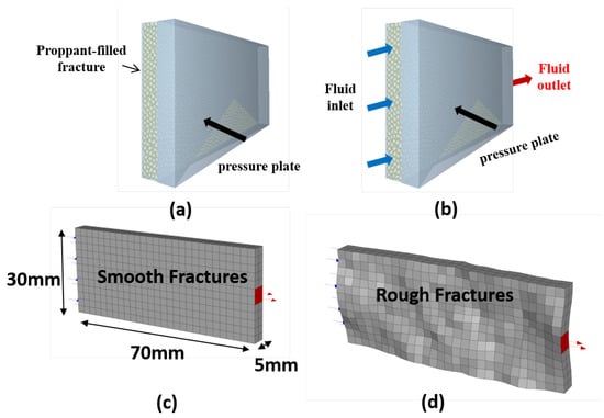
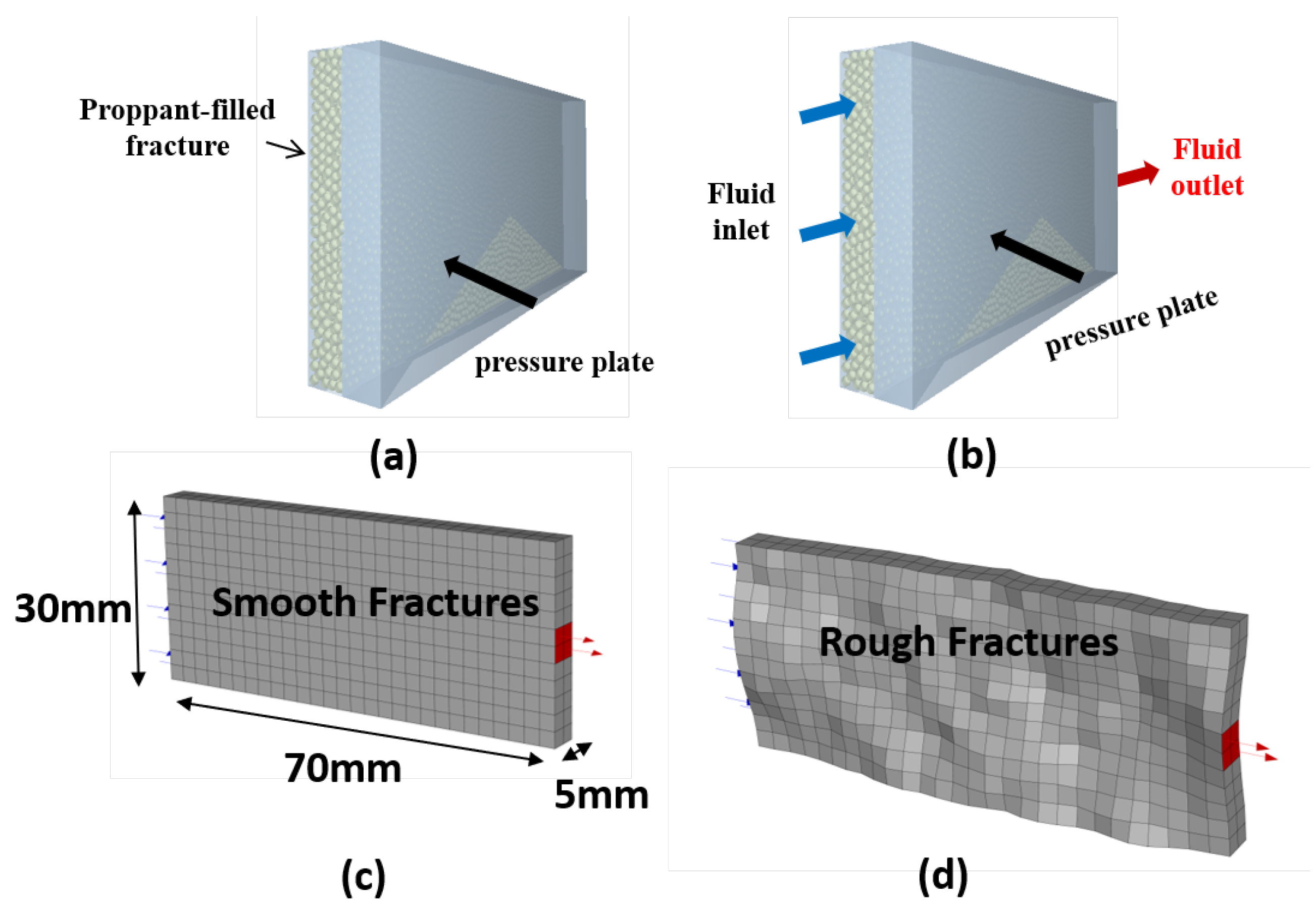
We used transient calculations for the simulated scenarios, including the scenarios with constant inlet velocity. The smooth-fracture model has 672 CFD cells in the structured arrangement shown in Figure 1 (Appendix B gives the supporting model details and limitations).

Figure 1. Schematics showing the simulation setup for (a) a proppant-filled fracture and (b) fluid flow through the fracture (modified after [14]); geometry, dimensions, and mesh schematics for (c) smooth and (d) rough fractures in CFD-DEM simulation.

The proppant flowback simulation followed four steps: particle filling, fracture closure, fluid flowback, and particle flowback. Figure 1a,b briefly shows the workflow. The model first filled proppant particles into the fracture to form an initial proppant pack. A pressure plate then loaded the fracture and simulated closure. Closure stress compacted the proppant and formed a stable particle skeleton. After mechanical stabilization, the model set a perforation outlet and a velocity inlet. The inlet velocity then increased gradually to observe proppant initiation, migration, and flowback-channel evolution.

We interpret the prescribed 0.5–25 MPa loads as net closure traction, ${\sigma }_{cl}={\sigma }_n-p_f$, where ${\sigma }_n$ is total normal stress and $p_f$ is fracture-fluid pressure (see Appendix B.3 for the loading limits).

We use an idealized local fracture model (see Appendix B.1 for definitions of the relevant dimensionless groups). Figure 1 shows the near-wellbore parallel-plate fracture model. The model domain measured ($70\mathrm{mm}\times 30\mathrm{mm}\times 5\mathrm{mm}$), with an inlet size of $70\mathrm{mm}\times 5\mathrm{mm}$ and an outlet size of $5\mathrm{mm}\times 5\mathrm{mm}$. We used this model to simulate proppant flowback near the perforation. We also compared smooth and rough fracture walls to evaluate the effect of wall roughness on proppant stability.

The simulation used quartz-sand proppant properties from the study area and coal-rock mechanical properties for the fracture walls. We applied a velocity inlet and a pressure outlet as boundary conditions. The Gidaspow drag model described fluid-particle interactions, and the DDPM interface coupled the fluid and particle phases. The fluid-phase time step was ($\begin{array}{c}\hfill 5\times {10}^{-4}\mathrm{s}\end{array}$), and the particle-phase time step was ($\begin{array}{c}\hfill 5\times {10}^{-6}\mathrm{s}\end{array}$). Table 2 summarizes the model parameters.

Table 2. Summary of inputs for CFD-DEM simulation.

Parameters	Value	Parameters	Value
Particle density ($\mathrm{kg}{\mathrm{m}}^{-3}$)	2650	Fluid density ($\mathrm{kg}{\mathrm{m}}^{-3}$)	1000
Particle Poisson’s ratio	0.3	Wall Poisson’s ratio	0.35
Particle Young’s modulus ($\mathrm{Pa}$)	$7\times {10}^{10}$	Wall Young’s modulus ($\mathrm{Pa}$)	$7\times {10}^9$
Particle-particle coefficient of restitution	0.5	Particle-wall coefficient of restitution	0.5
Particle-particle coefficient of static friction	0.75	Particle-wall coefficient of static friction	0.5
Particle-particle coefficient of rolling friction	0.02	Particle-wall coefficient of rolling friction	0.01
DEM time step ($\mathrm{s}$)	$5\times {10}^{-6}$	CFD time step ($\mathrm{s}$)	$5\times {10}^{-4}$

The simulation schemes used a single-factor control method. The critical proppant initiation velocity schemes analyzed proppant size, fracture width, fracture roughness, fracturing-fluid viscosity, and effective closure stress. The flowback quantity and flowback distribution schemes further evaluated proppant size, fracture width, fluid velocity, effective closure stress, and proppant embedment depth. Table 3 lists the specific inputs for 9 CFD-DEM simulation scenarios. In Scenarios 1 to 4, we set a fixed velocity gradient such that the fluid velocity at the inlet increases with time. In Scenarios 5 to 9, we set a fixed fluid velocity at the inlet for CFD-DEM simulations.

Table 3. Input parameter settings for the 9 CFD-DEM simulation scenarios.

Scenarios	Proppant Size ($\mathbf{mm}$)	Fracture Width ($\mathbf{mm}$)	Fracture Roughness	Effective Closure Stress ($\mathbf{MPa}$)	Fluid Velocity ($\mathbf{m}/\mathbf{s}$), t ($\mathbf{s}$)	Proppant Embedment Depth ($\mathbf{mm}$)
Scenario 1	$0.6/0.7/0.8/$$0.9/1$	5	Smooth	10	$0.1t$	0
Scenario 2	1	$2/3/4/5/6$	Smooth	10	$0.1t$	0
Scenario 3	1	5	Smooth/Rough	10	$0.1t$	0
Scenario 4	1	5	Smooth	$5/10/15/$$20/25$	$0.1t$	0
Scenario 5	$0.6/0.7/0.8/$$0.9/1$	5	Smooth	10	0.1	0
Scenario 6	1	$2/3/4/5/6$	Smooth	10	0.1	0
Scenario 7	1	5	Smooth	10	$0.02/0.05/0.1/$$0.2/0.3/0.5$	0
Scenario 8	1	5	Smooth	$0.5/10/15/$$20/25$	0.1	0
Scenario 9	1	5	Smooth	10	0.1	$0.1/0.2/0.3/$$0.4/0.5$

3.2. A Machine-Learning Workflow for Predicting Proppant Risks

We trained binary classifiers using field data from 73 deep-CBM wells. Nine wells had recorded surface sand production, while 64 did not. Predictors included static variables from Table 1 and time-series records of wellhead pressure, water rate, and choke size. We estimated missing static values using nearby-well data and field records. We standardized continuous variables using Z-scores.

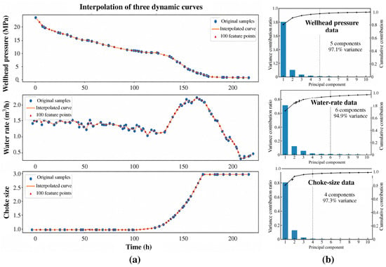
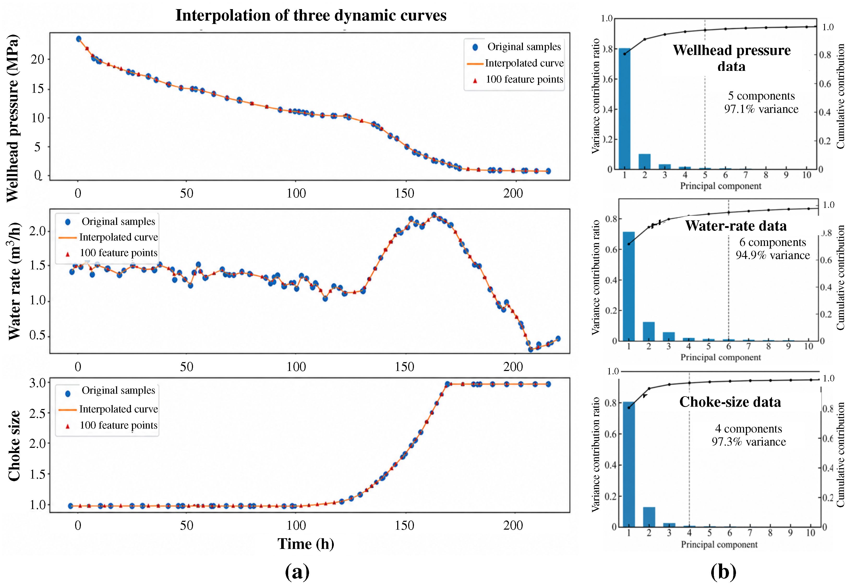
As illustrated by Figure 2a, flowback records varied in length. We thus interpolated each pressure, water-rate, and choke-size curve to 100 equally spaced points. We used principal component analysis (PCA) to reduce data dimensions. Five pressure components retained 97.1% of the variance. Six water-rate components retained 94.9%. Four choke-size components retained 97.3% (see Figure 2b).

Figure 2. Dynamic flowback feature extraction and PCA: (a) Interpolation of wellhead-pressure, water-rate, and choke-size curves to obtain 100 feature points per variable; (b) PCA results showing that 5, 6, and 4 principal components retain 97.1%, 94.9%, and 97.3% of the cumulative variance, respectively.

We employed the XGBoost and back-propagation neural network (BPNN) models for machine learning applications. We trained models using either static variables alone or a combination of static and dynamic variables. We evaluated each model using leave-one-well-out cross-validation (LOWO). Each iteration reserved one well for testing and used 72 wells for training. We repeated this process 73 times, allowing every well to serve once as an independent test sample.

We reported overall accuracy and the number of correct predictions for each class. We also calculated SHAP values for XGBoost models. Mean absolute SHAP values ranked each predictor’s contribution to model output.

4. Application and Results

In this section, we report the results of field-data analysis of proppant flowback. We further show the results of CFD-DEM simulation of proppant flowback. Finally, we present the machine-learning results for proppant flowback risks.

4.1. Field Observations of Proppant Flowback

4.1.1. Flowback Behaviors of Wells with Proppant Production

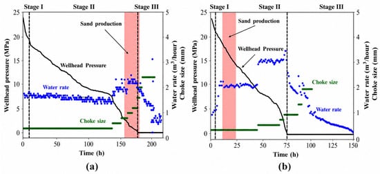
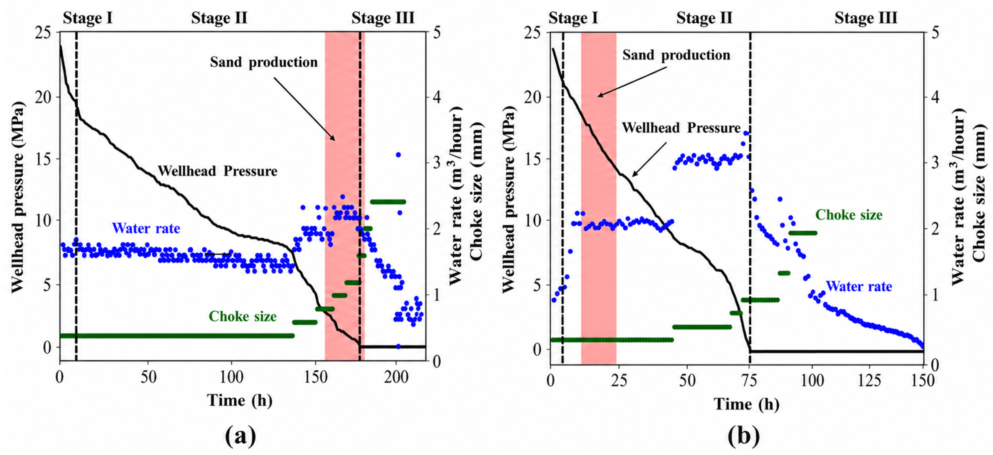
Figure 3a,b show the flowback data of water rate, casing pressure, and choke size for typical Linxing and Shenfu wells. In Figure 3, the red bands indicate the flowback hours of proppant production. According to the change in wellhead pressure, we divided the flowback of target wells into three stages: rapid pressure decline (Stage I), gradual pressure decline (Stage II), and near-atmospheric-pressure flowback (Stage III).

Figure 3. Typical flowback profiles of water rate, casing pressure, and choke size for (a) Linxing and (b) Shenfu wells. The dashed lines divide the flowback profiles into three stages: Stage I, Stage II, and Stage III. The red bands highlight the flowback hours with sand production.

(a)

Stage I describes the initial hours of flowback, which are characterized by a rapid drop in wellhead pressure. Operators initially maintain a low water rate using a small choke, typically about 2 mm. Stage I usually lasts several hours, during which wellhead pressure decreases by approximately 3–7 MPa. Cumulative water production generally remains below the wellbore volume during Stage I. Proppant production was reported in a limited number of wells during Stage I.

(b)

Stage II begins when the rate of wellhead-pressure decline slows, and continues until wellhead pressure approaches atmospheric pressure. Operators progressively enlarge the choke during Stage II, producing stepwise increases in water rate. Water rate often reaches its maximum during Stage II. Wellhead pressure initially decreases gradually, whereas the later increases in choke size and water rate accelerate the pressure decline. Most proppant production from the 12 investigated deep-CBM wells occurs during Stage II, identifying the intermediate flowback period as the primary stage of proppant flowback. Proppant flowback is mainly associated with changes in choke size or water rates.

(c)

During Stage III, flowback continues with wellhead pressure approaching atmospheric pressure. Operators continue to enlarge the choke, and eventually remove the flow restriction. The water rate then decreases progressively until water flow at the surface ceases. Then, the flowback operation ends with negligible water recovery. A limited number of wells produce proppant during Stage III.

4.1.2. Comparative Analysis of Proppant Flowback Behaviors

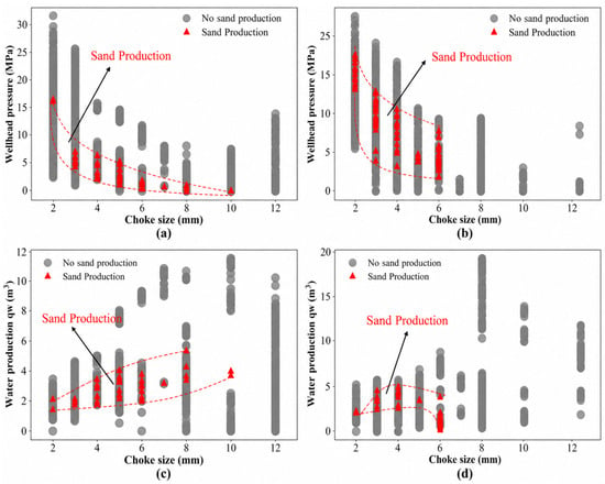
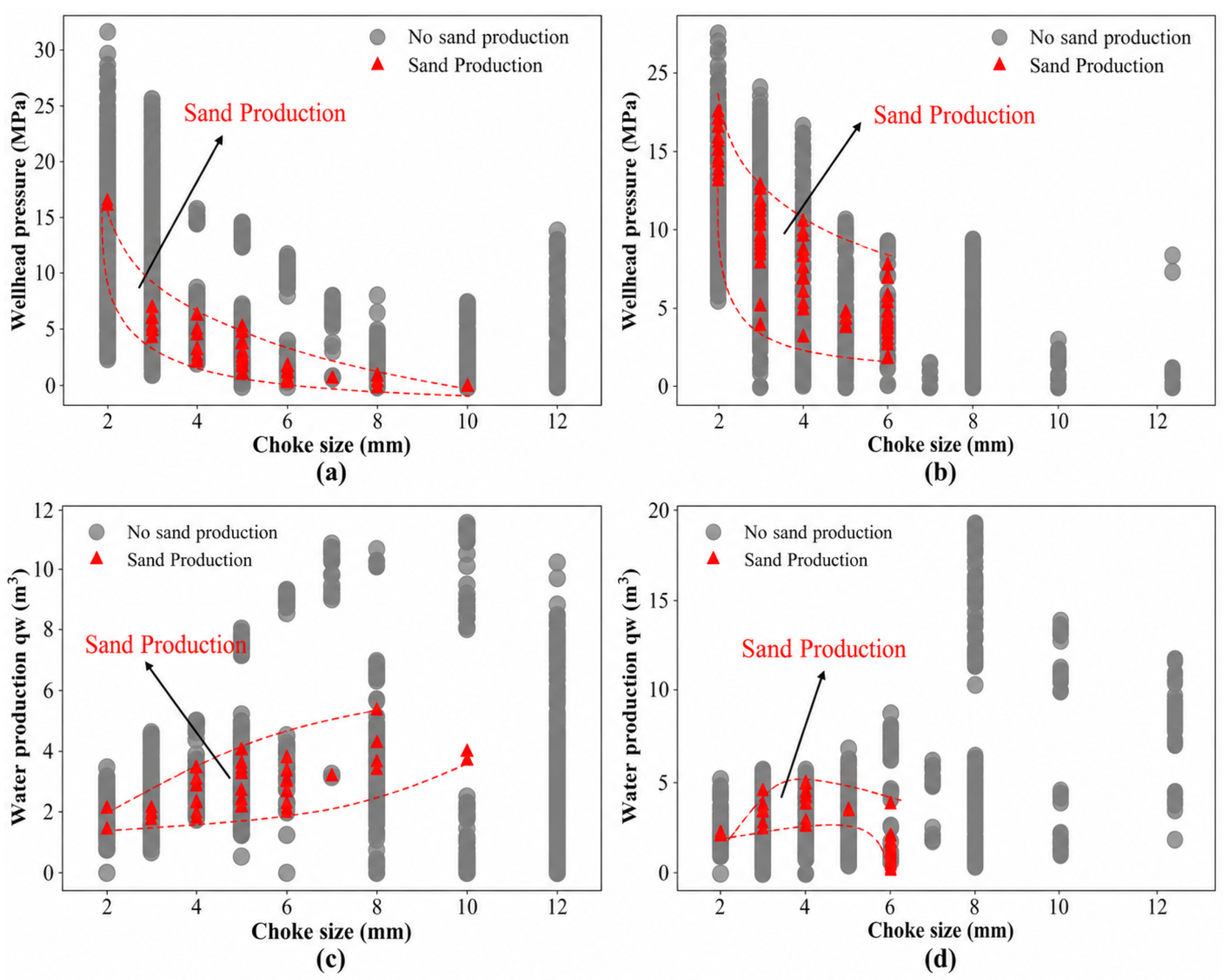
In Figure 4, we plot the flowback data of wellhead pressure and water rate against choke size for 12 target wells completed in the Linxing and Shenfu blocks, respectively. As highlighted in Figure 4, the proppant flowback generally clusters into patterns, which indicates flowback periods at a relatively high risk of proppant flowback.

Figure 4. Cross plot of flowback data of wellhead pressure versus choke size for (a) Linxing and (b) Shenfu wells, and flowback data of water rate versus choke size for (c) Linxing and (d) Shenfu wells. Flowback data with proppant production are colored in red. The dashed lines cluster the zone with proppant production.

Figure 4 shows the relationships among choke size, wellhead pressure, water production rate, and proppant flowback. The proppant flowback data points occupy relatively narrow regions within the full operating range, suggesting that no single parameter defines the onset of proppant flowback.

In Figure 4a,b, the wellhead pressure associated with proppant flowback decreases as the choke size increases. At small choke sizes of about 2–3 mm, proppant flowback can occur at relatively high wellhead pressures. At choke sizes of about 4–6 mm, most flowback events occur at lower pressures. Figure 4a shows the decreasing trend over a wider choke range for Linxing wells. In contrast, Figure 4b shows that most flowback events occur between 2 and 6 mm for Shenfu wells. The results define an approximate wellhead pressure-choke operating window for proppant flowback. The operating window for Linxing wells is relatively higher and wider compared with Shenfu wells.

Figure 4c,d show a similar operating-window behavior. In Figure 4c, the water rate associated with proppant flowback generally increases with choke size. In Figure 4d, most flowback events occur at choke sizes of 2–6 mm and at moderate water rates. However, a large portion of flowback data without any proppant flowback occurs at higher water rates and larger choke sizes. Therefore, high water rate alone does not trigger proppant flowback.

The highest flowback risk appears during Stage II with the intermediate choke-opening stage. At this stage, the well still maintains sufficient pressure and flow energy to mobilize proppant, while the enlarged choke promotes stronger fluid transport toward the wellbore. At later stages, larger choke sizes or higher water rates do not necessarily cause proppant flowback because the wellhead pressure has declined and part of the mobile proppant may already have been produced.

4.2. CFD-DEM Simulation

4.2.1. Results of Base Case

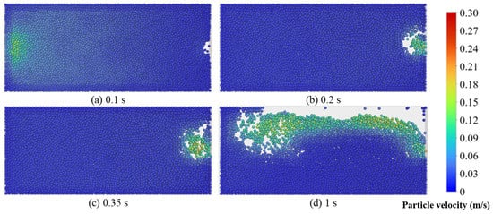
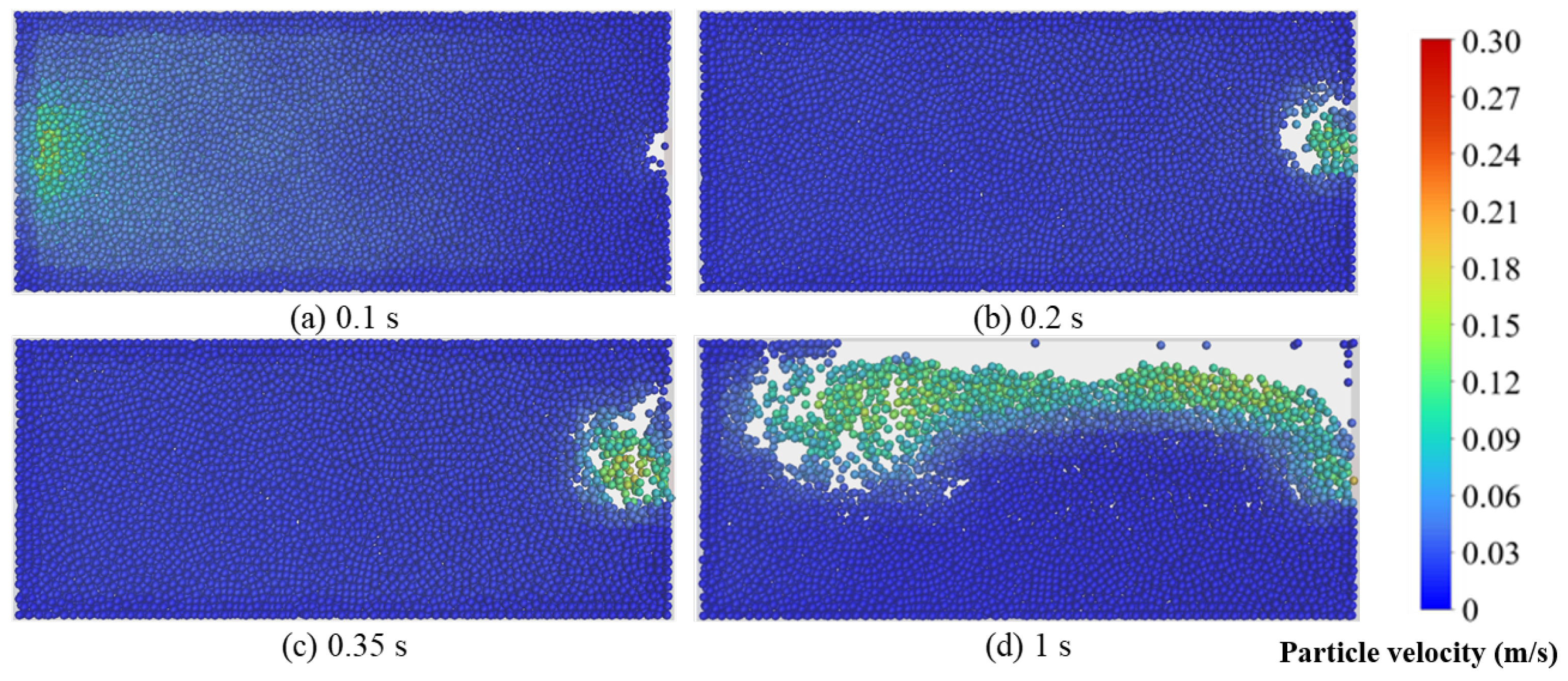
Figure 5 shows the progressive development of proppant flowback as the inlet velocity increases ($v=0.1t$) for Scenario 1 with a particle size of 1 mm (see Table 3). At 0.1 s, the proppant pack remains stable, and no obvious particle displacement occurs, indicating a stage without proppant flowback. At 0.2 s, fluid forces begin to mobilize loosely packed particles near the outlet, producing limited proppant loss during the slow-flowback stage. As the velocity continues to increase, particle motion becomes more pronounced, and the stable bridging structure gradually weakens. At about 0.35 s, the bridge collapses and triggers collective particle migration. A distinct flowback channel then develops along the upper part of the fracture, marking the onset of the rapid proppant flowback stage.

Figure 5. Proppant distribution and particle velocity (indicated by the color scale) inside the fracture at times from 0.1 to 1 s for Scenario 1 with a particle size of 1 mm.

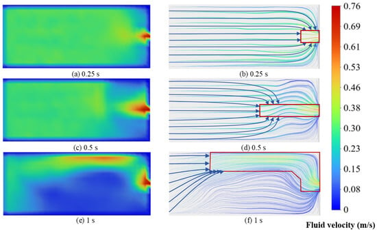
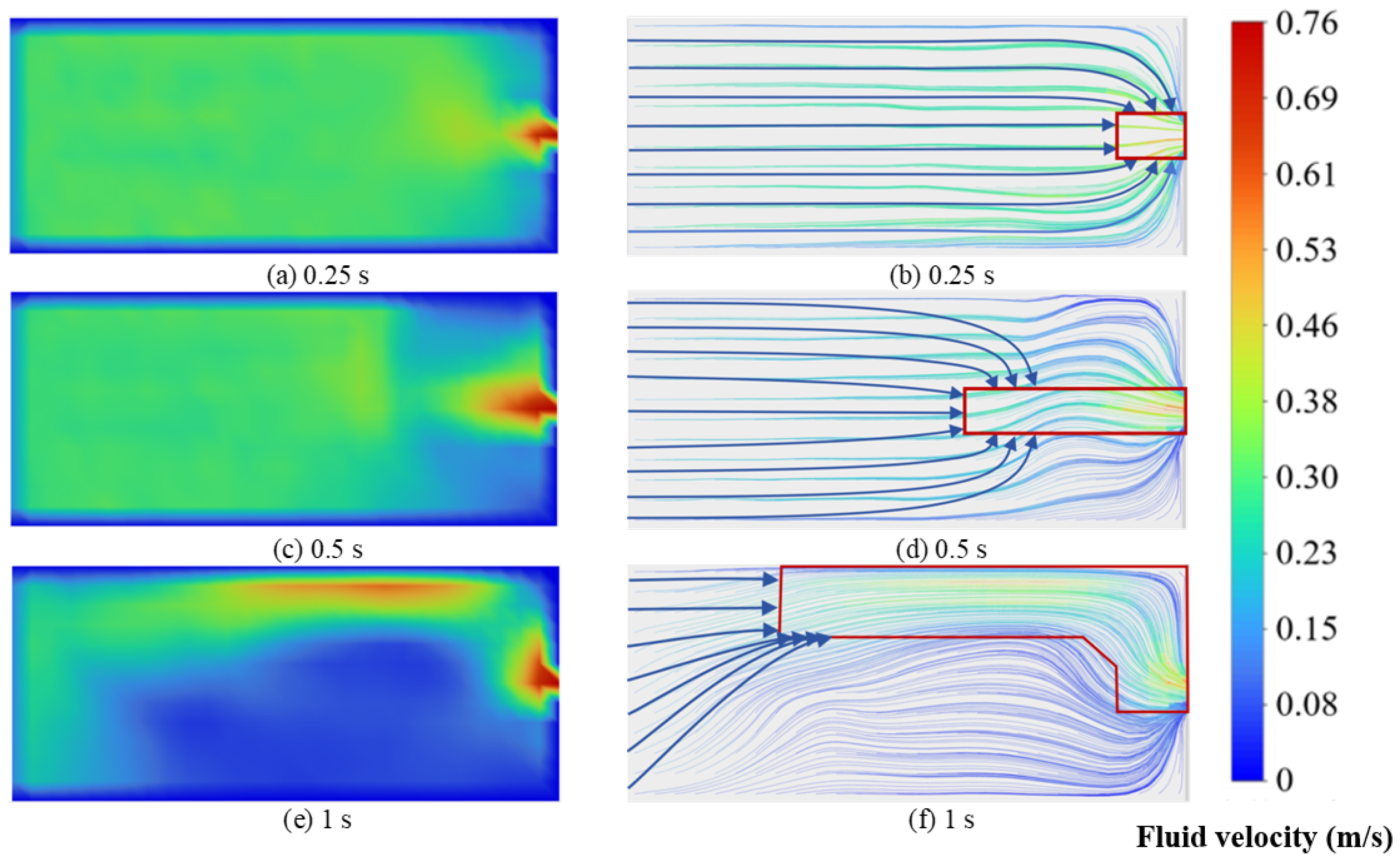
Figure 6 shows how fluid redistribution controls the development of a proppant flowback channel for a case in Scenario 1. As the fluid approaches the outlet, the streamlines converge and locally increase the flow velocity. This high-velocity zone first mobilizes proppant near the outlet and initiates a flowback channel. The channel then provides a preferential flow path and progressively expands as particles are removed from its boundary. As the open boundary enlarges, the average velocity along the channel boundary decreases. In the vertical fracture, the channel mainly propagates upward toward the inlet, while flowback below the outlet remains limited. The asymmetric development indicates that gravity promotes downward proppant settling and destabilizes the upper part of the proppant pack, causing particles above the outlet to flow back preferentially.

Figure 6. The change in particle velocity and streamlines of fluid flow during the proppant flowback process ((a), (c), and (e) show the particle velocity at 0.25, 0.5, and 1 s of simulation; (b), (d), and (f) show the streamlines of fluid flow at 0.25, 0.5, and 1 s of simulation. The red boxes highlight the development of proppant-flowback channels).

4.2.2. The Effects of Particle Size

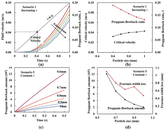
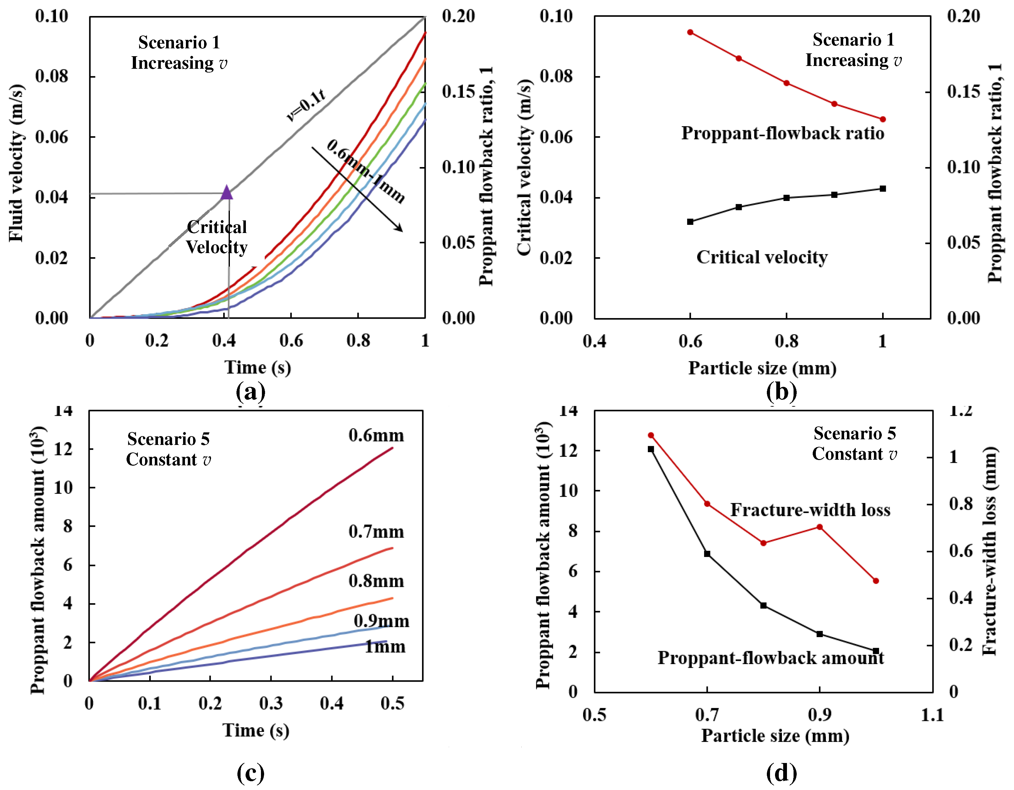
Figure 7 presents the simulated effects of particle size on proppant flowback behavior in deep-CBM wells for Scenarios 1 and 5. Figure 7a shows that the proppant flowback ratio increases continuously with time for all particle sizes in Scenario 1. Smaller particles exhibit a higher flowback tendency because they have lower critical velocities. The critical velocity increases with particle size, indicating that larger particles require higher fluid velocities to initiate particle transport. As shown in Figure 7b, the critical velocity increases from approximately 0.03 to 0.04 m/s as particle size increases from 0.6 to 1.0 mm, whereas the corresponding proppant flowback ratio decreases significantly.

Figure 7. Simulation results showing the effects of particle size on proppant flowback behaviors of deep-CBM wells: (a) Proppant flowback ratio versus time with varying particle size for Scenario 1 (the lines in black illustrate the critical velocity for the particle size of 1 mm); (b) Critical velocity and proppant flowback ratio as a function of particle size for Scenario 1; (c) The increase in proppant flowback amount against time at varying particle size for Scenario 5; (d) The proppant flowback amount and fracture-width loss as a function of particle size for Scenario 5.

Figure 7c further demonstrates that particle size strongly controls the accumulation rate of proppant flowback for Scenario 5. The flowback amount increases almost linearly with time, and smaller particles produce substantially higher flowback volumes. For example, the 0.6 mm particles generate the largest flowback amount, while the 1.0 mm particles show the lowest value. The results indicate that fine proppants are more easily mobilized under the same flow conditions.

Figure 7d summarizes the relationship between particle size, proppant flowback amount, and fracture-width loss for Scenario 5. Increasing particle size reduces both the flowback amount and fracture-width loss. The fracture-width loss decreases from approximately 1.1 mm for 0.6 mm particles to less than 0.5 mm for 1.0 mm particles. Meanwhile, the proppant flowback amount decreases by nearly 80%. These results indicate that larger proppant particles improve flowback control by increasing the critical transport velocity and reducing particle migration.

4.2.3. The Effects of Fracture Width

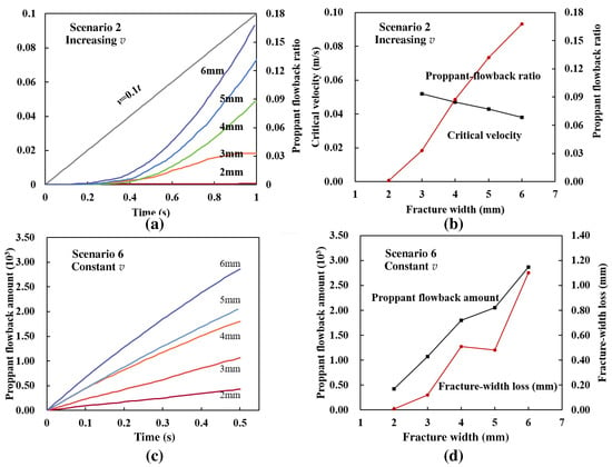
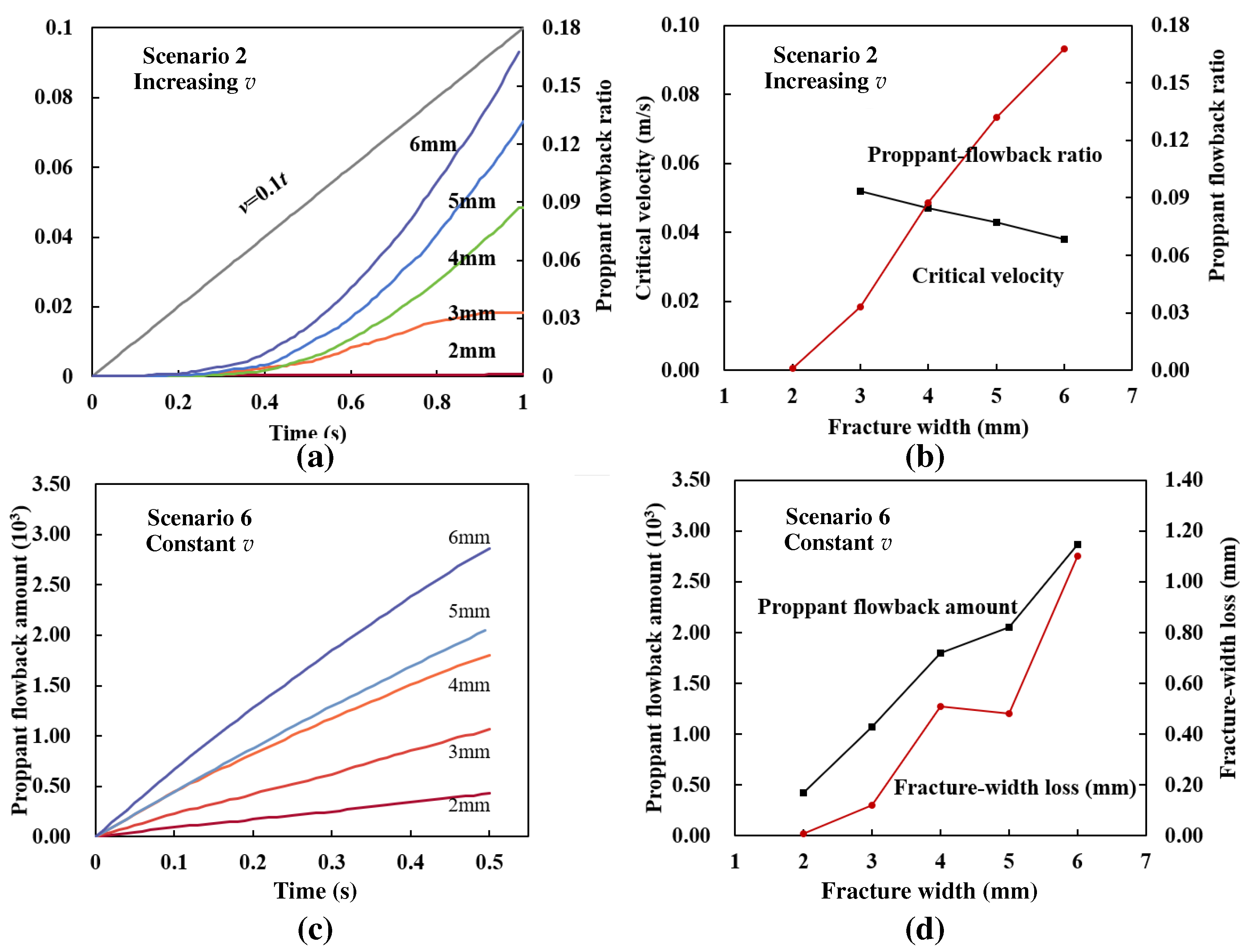
Figure 8 shows that fracture width strongly affects proppant flowback for Scenarios 2 and 6. The aperture sweep gives $b_0/d_p=2$–6 for $d_p=1\mathrm{mm}$. Here, $b_0$ is the nominal geometric aperture before loading, not the hydraulic aperture. Packing and initial particle inventory also affect the comparison (see Appendix B.3). In Figure 8a, the fluid velocity increases linearly with time for Scenario 2. Proppant flowback starts once the fluid velocity reaches the transport condition for each fracture width. Wider fractures show an earlier onset and a higher flowback ratio. The 2 mm fracture shows almost no proppant flowback. In contrast, the flowback ratio reaches approximately 0.17 for the 6 mm fracture at the end of the simulation.

Figure 8. Simulation results showing the effects of nominal aperture $b_0$ ($b_0/d_p=2$–6; $d_p=1\mathrm{mm}$) on proppant flowback behaviors: (a) Proppant flowback ratio versus time with varying fracture width for Scenario 2 (the line in black illustrates the fluid velocity); (b) Critical velocity and proppant flowback ratio as a function of fracture width for Scenario 2; (c) The increase in proppant flowback amount against time at varying fracture width for Scenario 6; (d) The proppant flowback amount and fracture-width loss as a function of fracture width for Scenario 6.

Figure 8b shows the opposite trends in critical velocity and flowback ratio. The critical velocity decreases as the fracture width increases. It drops from about 0.052 m/s at 3 mm to about 0.038 m/s at 6 mm. Meanwhile, the proppant flowback ratio increases from nearly zero at 2 mm to approximately 0.17 at 6 mm. Thus, a wider fracture allows proppant particles to become mobile at a lower fluid velocity and increases the risk of flowback.

Figure 8c further shows that the cumulative flowback amount increases almost linearly with time for Scenario 6. The flowback rate also increases with fracture width. At 0.5 s, the flowback amount rises from about ($0.4\times {10}^3$) for the 2 mm fracture to nearly ($2.9\times {10}^3$) for the 6 mm fracture.

Figure 8d shows that the final flowback amount generally increases with fracture width. Fracture-width loss shows a similar overall trend, although a small decrease occurs from 4 to 5 mm. The width loss then increases sharply at 6 mm and reaches approximately 1.1 mm. These results indicate that wide fractures provide less confinement to the proppant pack. They therefore promote particle mobilization, increase proppant loss, and cause greater loss of the propped fracture width.

4.2.4. The Effects of Fracture Roughness

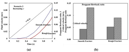
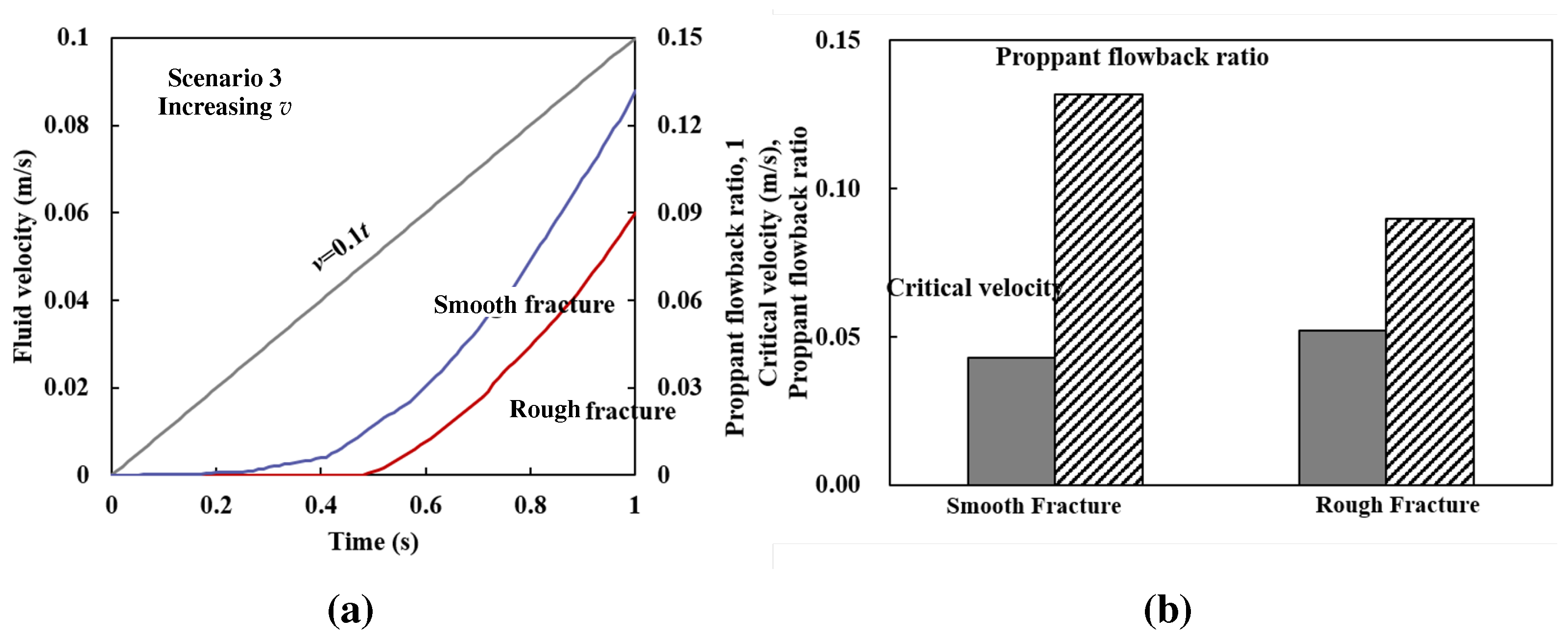
Figure 9 shows that fracture roughness suppresses proppant flowback in Scenario 3 (see Appendix B.2 for the surface-generation method and the missing roughness statistics). Proppant starts to flow back later in the rough fracture than in the smooth fracture. The critical velocity increases from approximately 0.043 $\mathrm{m}{\mathrm{s}}^{-1}$ for the smooth fracture to 0.052 $\mathrm{m}{\mathrm{s}}^{-1}$ for the rough fracture, while the final proppant flowback ratio decreases from about 0.13 to 0.09. These results indicate that fracture roughness increases particle confinement and flow resistance, thereby improving proppant-pack stability and reducing proppant mobilization during flowback.

Figure 9. Simulation results showing the effects of fracture roughness on proppant flowback behaviors of deep-CBM wells in Scenario 3: (a) Time evolution of flowback ratio for the smooth and rough geometries, with the imposed inlet velocity; (b) Bar chart comparing the critical velocity and proppant flowback ratio for smooth and rough fractures.

4.2.5. The Effects of Fluid Velocity

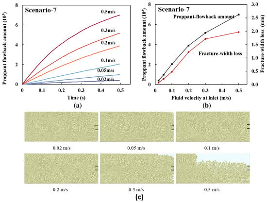
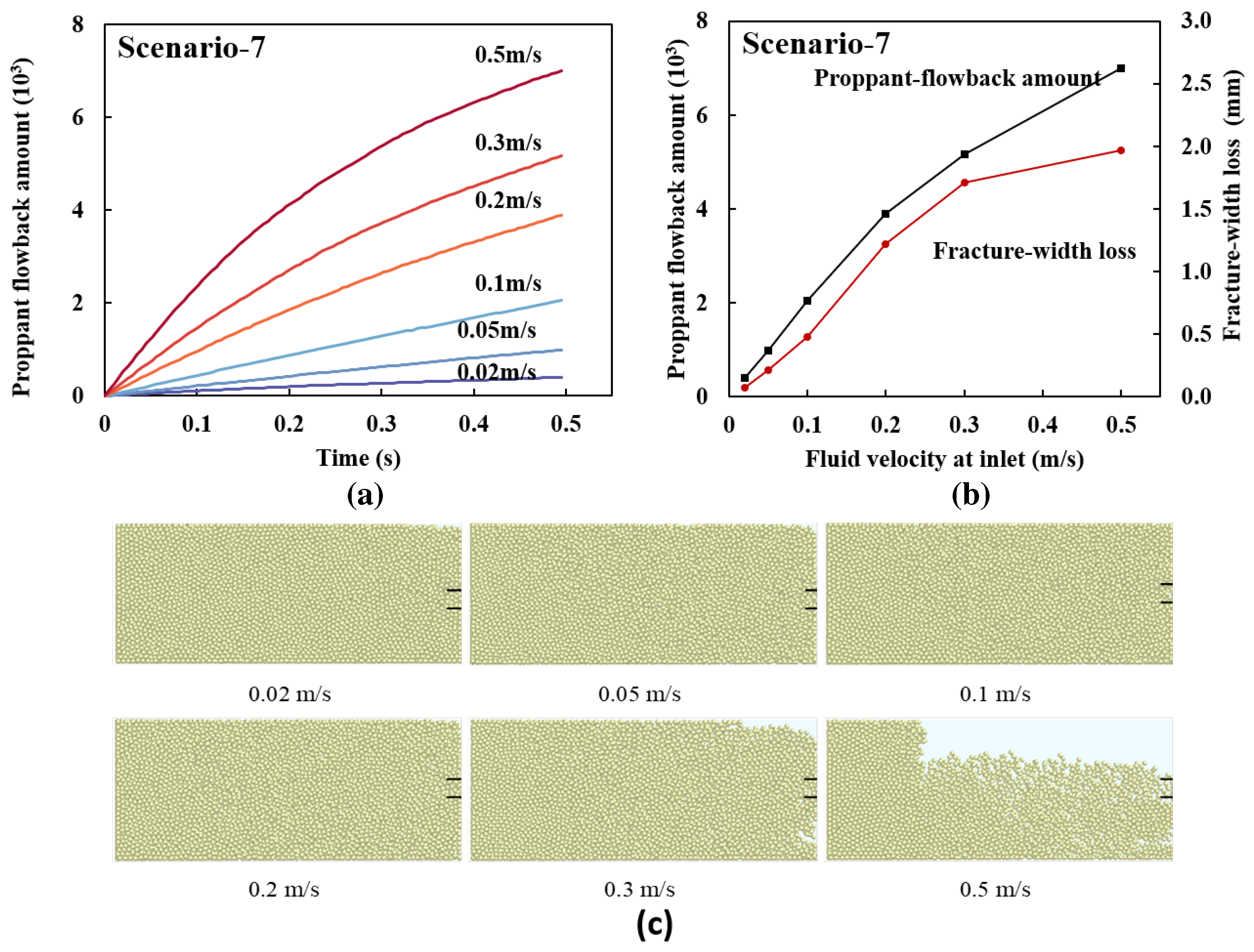
Figure 10 shows that increasing the inlet fluid velocity strongly promotes proppant flowback for Scenario 7. The cumulative flowback amount increases continuously with time and rises from approximately $0.3\times {10}^3$ at 0.02 m/s to about $7.0\times {10}^3$ at 0.5 m/s. Fracture-width loss also increases with fluid velocity and reaches about 2.0 mm at 0.5 m/s. The final particle distributions show increasingly large proppant-depleted zones at higher velocities. These results indicate that a higher fluid velocity increases the drag force on proppant particles, enhances particle mobilization, and causes greater proppant loss and fracture-width reduction.

Figure 10. Simulation results showing the effects of fluid velocity at the inlet on proppant flowback for Scenario 7: (a) The proppant flowback amount increases with time with varying fluid velocity; (b) The proppant flowback amount and fracture width loss as a function of fluid velocity at the inlet; (c) The distribution of proppant in fractures for varying fluid velocity at the end of the simulation.

4.2.6. The Effects of Effective Closure Stress

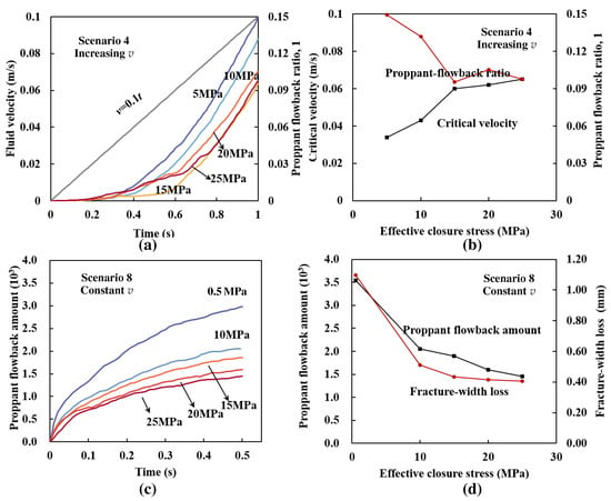
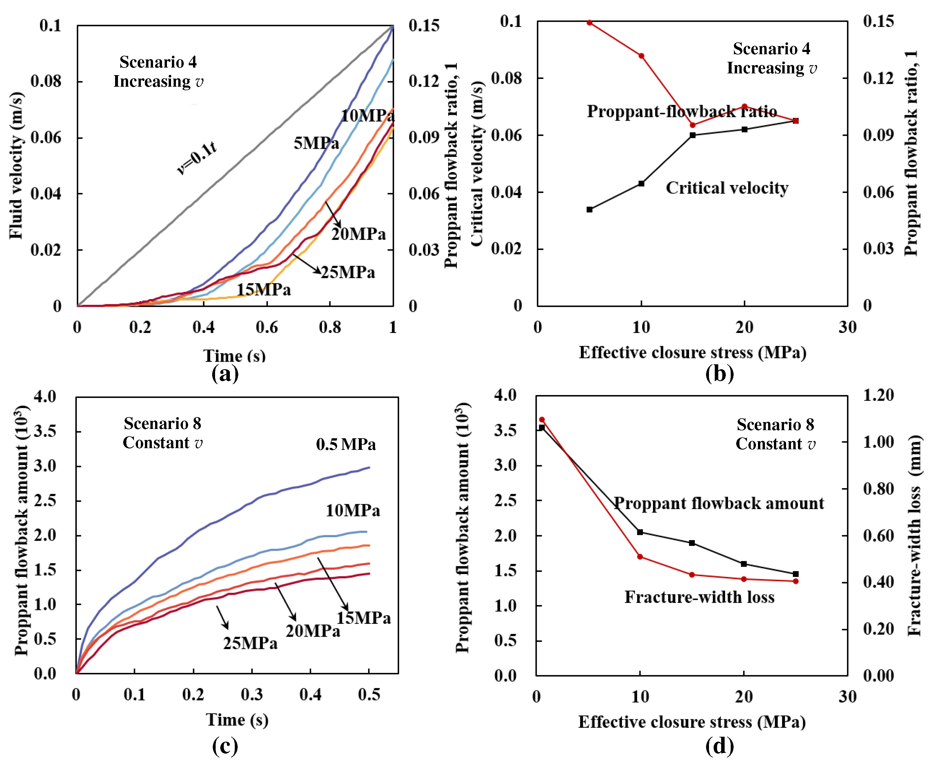
Figure 11 shows that effective closure stress strongly affects proppant flowback in Scenarios 4 and 8. In Figure 11a, the proppant flowback ratio increases with time under all stress conditions. Lower closure stress produces a higher flowback ratio. At 5 MPa, the flowback ratio reaches about 0.15 at the end of the simulation. Increasing the closure stress generally suppresses proppant flowback.

Figure 11. Simulation results showing the effects of effective closure stress on proppant flowback behaviors of deep-CBM wells: (a) Proppant flowback ratio versus time with varying effective closure stress (the line in black illustrates the fluid velocity) for Scenario 4; (b) Critical velocity and proppant flowback ratio as a function of effective closure stress for Scenario 4; (c) The increase in proppant flowback amount against time at varying effective closure stress for Scenario 8; (d) The proppant flowback amount and fracture-width loss as a function of effective closure stress for Scenario 8.

Figure 11b shows that the critical velocity increases with effective closure stress. It rises from approximately 0.034 m/s at 5 MPa to about 0.065 m/s at 25 MPa. In contrast, the proppant flowback ratio generally decreases as the closure stress increases. The ratio drops sharply between 5 and 15 MPa, followed by a small increase at 20 MPa and a slight decrease at 25 MPa. These results indicate that higher closure stress requires a higher fluid velocity to mobilize the proppant.

Figure 11c further shows that the cumulative flowback amount increases continuously with time. However, its magnitude decreases with increasing closure stress. At 0.5 s, the flowback amount decreases from approximately ($3.0\times {10}^3$) at 0.5 MPa to about ($1.5\times {10}^3$) at 25 MPa. The difference becomes more pronounced as flowback proceeds.

Figure 11d shows similar trends in the final flowback amount and fracture-width loss. Both decrease as effective closure stress increases. The fracture-width loss drops rapidly from about 1.1 mm at 0.5 MPa to approximately 0.5 mm at 10 MPa. It then decreases more gradually at higher stresses. These results suggest that increasing closure stress strengthens proppant confinement and improves the stability of the proppant pack. This effect raises the critical transport velocity and reduces both proppant loss and fracture-width loss.

4.2.7. The Effects of Fracture Embedment

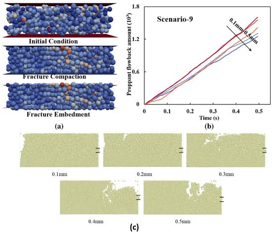
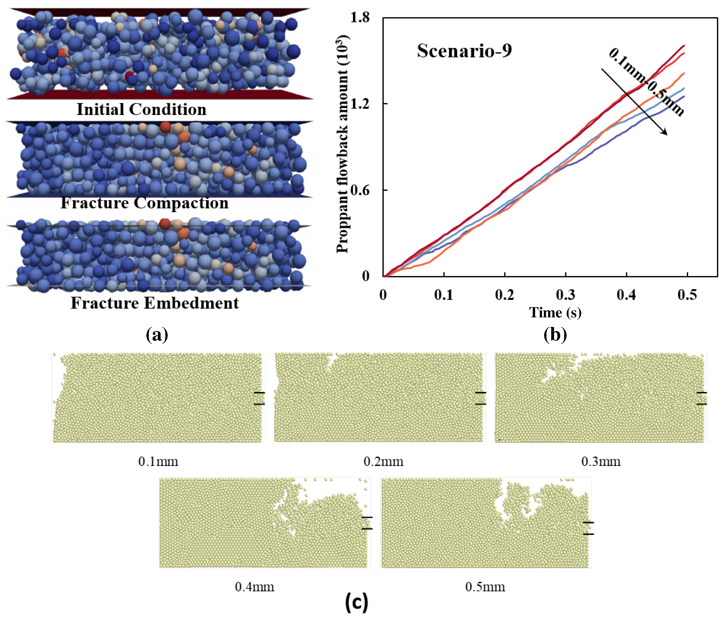
Figure 12 shows that fracture embedment suppresses proppant flowback for Scenario 9. Fracture compaction forces proppant particles into the fracture surfaces and increases particle confinement. As the embedment depth increases from 0.1 to 0.5 mm, the cumulative proppant flowback amount decreases. The final particle distributions also show less proppant depletion at greater embedment depths. These results indicate that deeper embedment stabilizes the proppant pack and reduces particle mobilization during flowback.

Figure 12. Simulation results showing the effects of fracture embedment on proppant flowback for Scenario 9: (a) Schematic illustrating the process of fracture embedment due to fracture compaction; (b) The proppant amount increases with time with varying fracture-embedment depth; (c) The distribution of proppant in fractures for varying fracture-embedment depth at the end of the simulation.

4.3. Field-Based Prediction of Proppant Flowback Risk

Table 4 lists the prediction performance of different feature combinations using XGBoost and BPNN. XGBoost with static features correctly identifies 5 of 9 sand-producing wells and 57 of 64 non-sand-producing wells. Adding the flowback dynamic parameters of pressure (startup pressure and pressure-decline curve characterized by PCA) produces the highest accuracy of 94.52%, with 7 of 9 sand-producing wells and 62 of 64 other wells correctly identified (see Appendix C, which reports all class-sensitive metrics, uncertainty intervals, and the limitations).

Table 4. Proppant flowback predictions using different features by XGBoost and BPNN.

Input Features	Model	Sand Wells	Non-Sand Wells
Static features	XGBoost	5	57
Static features	BPNN	2	58
Static + startup pressure + choke variation	XGBoost	4	59
Static + startup pressure + liquid production	XGBoost	6	61
Static + startup pressure + pressure decline	XGBoost	7	62
All features	XGBoost	6	59

In contrast, adding the dynamic parameters extracted from the liquid-production curve, choke-variation curve, or all dynamic features reduces the accuracy. XGBoost consistently outperformed BPNN. With static features, BPNN identified only two of nine sand-producing wells. The results indicate that static parameters and features extracted from the pressure-decline curve using PCA provide the most useful dynamic information for proppant flowback prediction.

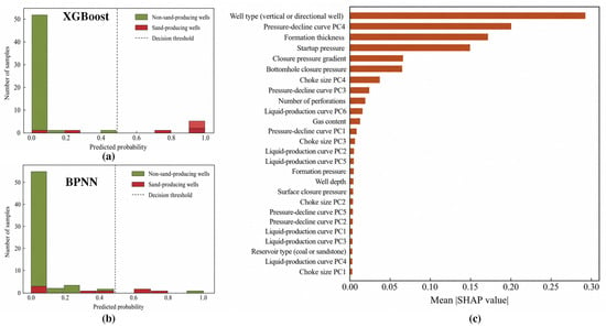
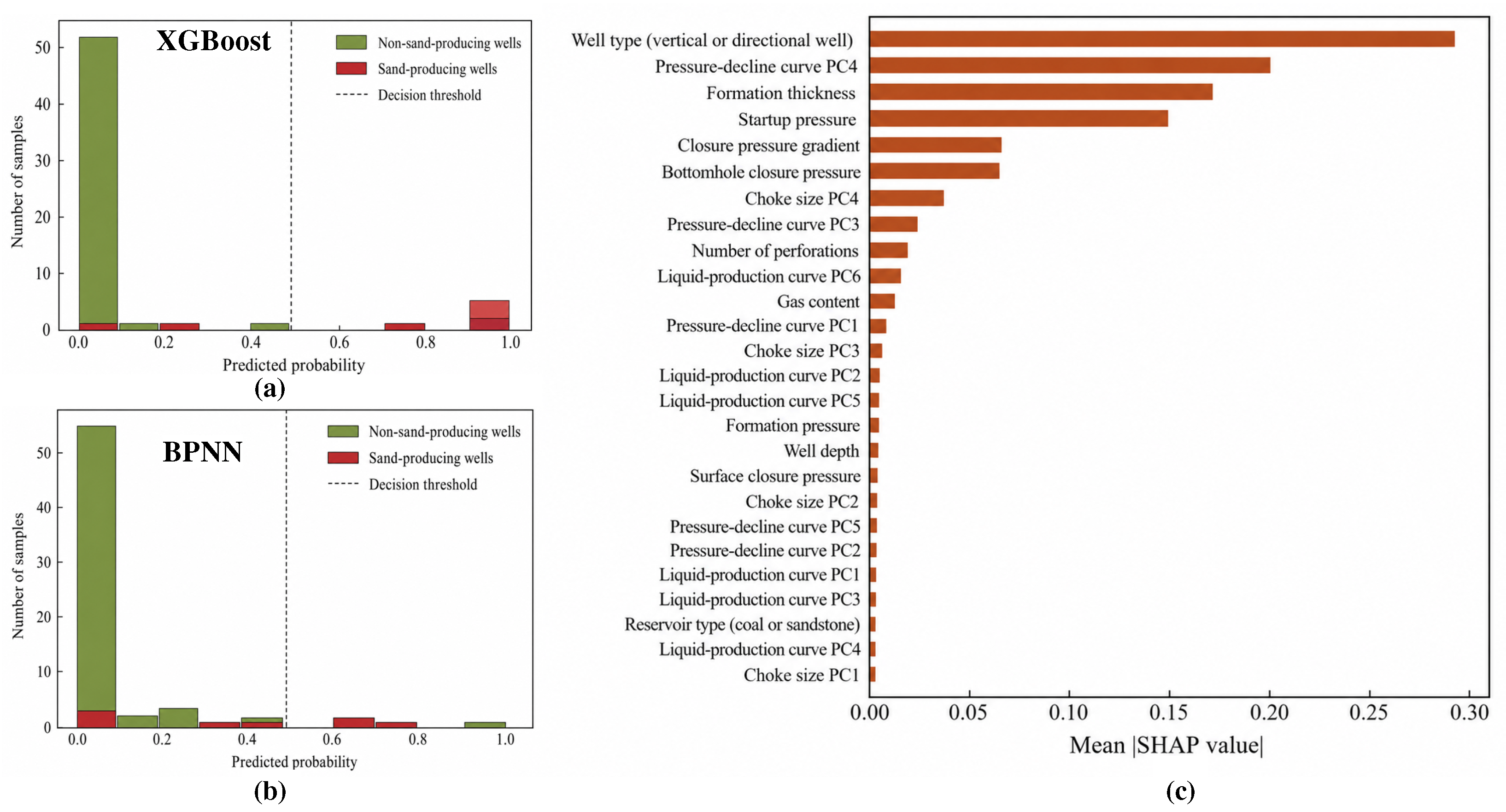
Figure 13 compares the predicted probability distributions of XGBoost and BPNN for proppant flowback classification. XGBoost provides a clearer separation between sand-producing and non-sand-producing wells. Most non-sand-producing wells show probabilities close to zero, whereas sand-producing wells mainly exhibit high predicted probabilities. In contrast, BPNN produces a wider probability distribution with greater overlap between the two classes, indicating weaker classification performance.

Figure 13. Field sand-production classification and feature-importance analysis. Predicted probabilities of recorded sand production by (a) XGBoost using static parameters and dynamic flowback-pressure data and (b) BPNN using static parameters and startup pressure. Green bars represent wells without sand production. Red bars represent sand-producing wells. (c) Feature importance is ranked by the mean absolute SHAP values from the XGBoost model for input features.

The SHAP analysis identifies the relative contributions of static and dynamic features in the XGBoost model. These feature rankings describe associations with recorded sand production. Among all input variables, well type shows the highest importance, followed by the dynamic pressure-decline curve PC4, formation thickness, and startup pressure. Other important features include closure-pressure gradient, bottomhole closure pressure, and dynamic choke-size curve PC4. The dynamic features, including pressure-decline PCs, choke-size PCs, liquid-production PCs, and startup pressure, provide additional information beyond static reservoir and completion parameters.

5. Discussion and Limitations

Field observations show that proppant flowback mainly occurs during Stage II. During Stage I, operators use a small choke and maintain a low water rate. During Stage III, wellhead pressure has already declined to a low level. Stage II combines sufficient pressure with progressive choke enlargement. Such conditions increase hydraulic forcing near fractures and create a higher risk of proppant mobilization. Previous studies also show that rapid drawdown and aggressive choke opening can increase proppant production [24,26]. Flowback risk therefore depends on coupled changes in pressure, choke size, and water rate rather than on a single critical choke size.

CFD-DEM results explain field observations at the particle scale. Fluid converges near the outlet and creates a local high-velocity zone. Flow first removes weakly confined particles near the outlet. Continued particle loss weakens local bridging and forms a preferential flowback channel. Fluid then concentrates inside the channel and promotes further erosion along channel boundaries. Previous numerical studies reported similar particle mobilization and channel-development behavior [12,16,17,18]. Such behavior explains rapid proppant production after pack destabilization begins.

Hydraulic forcing and mechanical confinement jointly control proppant stability. Higher fluid velocity and wider fractures promote particle transport. Larger particles, higher effective closure stress, greater wall roughness, and deeper embedment improve pack stability. Particle size and fracture width mainly control geometric confinement and bridging. Closure stress increases particle contact and friction. Rough fracture surfaces increase particle-wall resistance. Previous numerical and experimental studies report similar effects [12,16,17,18,26]. No single parameter therefore controls proppant flowback under all conditions.

Machine-learning results support field and simulation observations. Startup pressure, formation thickness, pressure-decline characteristics, choke variation, and well type show strong contributions to field-scale flowback prediction. Pressure-decline features provide especially useful dynamic information. Simulation-based models identify effective closure stress as an important control on critical velocity, while particle size and fluid velocity strongly affect cumulative flowback. Different feature rankings reflect different physical scales. Field variables describe hydraulic loading at surface and well scale. CFD-DEM variables describe particle resistance and local transport inside fractures. Combined results connect operating conditions with particle-scale flowback mechanisms.

Results also provide practical guidance for flowback management. Operators should avoid rapid choke enlargement while wells retain high pressure. Pressure decline and choke trajectory should be considered together during choke adjustment. A fixed choke-size limit cannot represent all wells because reservoir pressure, fracture geometry, completion design, and proppant properties vary among wells [24,25,26]. A dynamic operating window based on pressure, choke size, and production rate provides a more practical approach for controlling flowback risk.

Field data include 73 wells, of which only 9 are sand-producing wells, which limits statistical confidence in machine-learning predictions. Surface solids may also contain formation-derived particles; recorded sand production may not always represent returned proppant. Surface observations lag behind downhole particle movement because particles require transport time through the wellbore. Dynamic features extracted from complete flowback histories may also contain information recorded after sand production begins. CFD-DEM simulations use simplified fracture geometry, prescribed boundary conditions, and single-factor parameter variations. Also, the CFD-DEM simulation can be improved through further examinations of numerical independence and contact calibration. Future work should include more sand-producing wells, independent field validation, multivariable CFD-DEM designs, and direct conversion between surface operating conditions and near-wellbore flow velocity.

6. Summary and Conclusions

This study integrates field observations, CFD-DEM simulations, and machine learning to investigate proppant flowback in deep-CBM wells. The combined approach links field-scale operating conditions with particle-scale transport mechanisms. The main conclusions are as follows:

(1)

Proppant flowback mainly occurs during the intermediate flowback stage (Stage II). Progressive choke enlargement under sufficient wellhead pressure increases hydraulic forcing and promotes proppant mobilization. Flowback risk depends on the combined effects of pressure decline, choke variation, and water production rather than a single operating parameter.

(2)

CFD-DEM simulations reveal the evolution of proppant flowback. Particle movement initiates near the fracture outlet, where local fluid velocity increases. Particle loss weakens the stable pack and forms a preferential flowback channel, which accelerates further proppant migration.

(3)

Hydraulic conditions and mechanical confinement jointly control proppant stability. Higher fluid velocity and wider fractures increase flowback, whereas larger particles, higher closure stress, rougher fracture surfaces, and deeper embedment improve proppant retention.

(4)

Dynamic flowback data improve proppant-risk prediction, while static geological and completion parameters remain dominant controls. The XGBoost model achieved the best performance by combining static features with pressure-related dynamic features. SHAP analysis identified well type, formation thickness, closure-related parameters, startup pressure, and pressure-decline characteristics as key predictors.

(5)

The results support dynamic choke management and risk-based flowback optimization for deep-CBM development. Future studies should include larger field datasets and more detailed near-wellbore flow simulations to improve prediction reliability.

Appendix A.1. Sampling and Measurement Methods

We sampled flowback fluid from LX-24D, LX-2H, and LX-3H between 0.5 and 144 h. We filtered and dried the solids, removed magnetic iron debris, and washed the samples. For laser particle-size analysis, we treated samples with peroxide and acid, then dispersed and sonicated them. The measurements therefore characterize treated solids. Only the LX-3H samples collected at 96 and 144 h yielded enough material for this analysis.

Appendix A.2. Particle-Size Results and Interpretation

Table A1 lists the measured percentiles. The main peaks fall within 200–400 $\mathsf{\mu }\mathrm{m}$. We define $D_n$ as the diameter below which n% of the measured particle volume occurs. The 144 h sample has lower $D_1$ and $D_5$ values and higher $D_{95}$ and $D_{99}$ values than the 96 h sample. Its distribution is broader, while $D_{50}$ changes little. Choke enlargement, particle collision and abrasion, and formation-fines migration offer possible explanations. The measured sizes overlap the injected proppant sizes.

Table A1. Particle-size percentiles for produced solids from LX-3H at 96 and 144 h. All diameters are in $\mathsf{\mu }\mathrm{m}$.

Time (h)	${\mathit{D}}_1$	${\mathit{D}}_5$	${\mathit{D}}_{16}$	${\mathit{D}}_{25}$	${\mathit{D}}_{50}$	${\mathit{D}}_{75}$	${\mathit{D}}_{84}$	${\mathit{D}}_{95}$	${\mathit{D}}_{99}$
96	2	21.8	135	156	205	264	295	361	424
144	1.07	8.45	99.5	136	207	290	335	430	511

Table A1. Particle-size percentiles for produced solids from LX-3H at 96 and 144 h. All diameters are in $\mathsf{\mu }\mathrm{m}$.

Time (h)	${\mathit{D}}_1$	${\mathit{D}}_5$	${\mathit{D}}_{16}$	${\mathit{D}}_{25}$	${\mathit{D}}_{50}$	${\mathit{D}}_{75}$	${\mathit{D}}_{84}$	${\mathit{D}}_{95}$	${\mathit{D}}_{99}$
96	2	21.8	135	156	205	264	295	361	424
144	1.07	8.45	99.5	136	207	290	335	430	511

Appendix B.1. Similarity Parameters

We use a reduced near-perforation model with a nominal size of $70\times 30\times 5\mathrm{mm}$. The inlet measures $70\times 5\mathrm{mm}$ and the outlet measures $5\times 5\mathrm{mm}$. The domain is an idealized local model. Let $b_0$ denote nominal geometric aperture, $d_p$ particle diameter, U inlet velocity, and $\mu$ dynamic viscosity. We use the following reference groups to describe the modeled regime:

$$R{e}_b={\displaystyle \frac{{\rho }_{f}U{b}_0}{\mu }},R{e}_p={\displaystyle \frac{{\rho }_{f}U{d}_p}{\mu }},S{t}_b={\displaystyle \frac{{\rho }_p{d}_p^{2}U}{18\mu b_0}}.$$

(A1)

For $b_0=5\mathrm{mm}$, $d_p=1\mathrm{mm}$, $U=0.1\mathrm{m}{\mathrm{s}}^{-1}$, and $\mu =1\mathrm{mPa}\mathrm{s}$, these groups are $R{e}_b=500$, $R{e}_p=100$, and $S{t}_b=2.94$. The density ratio is ${\rho }_p/{\rho }_f=2.65$. The nominal aperture ratio is $b_0/d_p=5$. The Stokes number uses the Stokes relaxation time as a reference scale; the solver retains Gidaspow drag.

Full similarity also requires matching confinement, shear forcing, and contact loading. Relevant groups include $b_0/d_p$, the Shields-type ratio ${\tau }_w/\left[({\rho }_p-{\rho }_f)g{d}_p\right]$, and ${\sigma }_{cl}/E_p$. Here ${\tau }_w$ is wall shear stress, ${\sigma }_{cl}$ is closure loading, and $E_p$ is particle Young’s modulus. For the listed loads, ${\sigma }_{cl}/E_p$ ranges from $7.14\times {10}^{-6}$ to $3.57\times {10}^{-4}$.

Appendix B.2. Rough-Surface Generation

We generated the rough surface with SynFrac and prepared the geometry with Rhino and SpaceClaim. SynFrac uses two random seeds. The available record does not retain their values, a surface-height map, or quantitative roughness parameters. We cannot recover root-mean-square height, correlation length, or relative roughness from the schematic. The comparison therefore describes one rough realization, not a calibrated roughness law.

Appendix B.3. Closure Loading and Aperture

We first fill the fracture with particles. We then apply normal pressure through a loading plate to compact the pack. After mechanical stabilization, we export the wall geometry and particle arrangement. We then activate the perforation outlet and fluid inlet for flowback.

We take compression as positive. At a fluid-filled fracture face, the net closure traction is ${\sigma }_{cl}={\sigma }_n-p_f$, where ${\sigma }_n$ is total normal stress and $p_f$ is fracture-fluid pressure. Bulk-rock effective stress follows ${\sigma }_n^{\prime }={\sigma }_n-{\alpha }_{B}p$, where ${\alpha }_B$ is the Biot coefficient and p is pore pressure. We interpret the 0.5–25 MPa values as separate net normal-loading cases for the particle pack. A plate load satisfies $F_n={\sigma }_{cl}A$, where A is the loaded area. A prescribed net traction already accounts for fluid pressure. Subtracting that pressure again would count it twice. The recorded setup documents pack preloading and export.

In the field, pressure decline can increase effective closure stress and change aperture. Our separate loading cases do not reproduce that coupled history. In Table 3, fracture width denotes the nominal geometric aperture used to set up each case, $b_0$. It is not a measured hydraulic aperture. We do not have the equilibrated aperture for every loaded pack.

References

- Li, X.; Wang, Y.; Jiang, Z.; Chen, Z.; Wang, L.; Wu, Q. Progress and study on exploration and production for deep coalbed methane. J. China Coal Soc. 2016, 41, 24–31. [Google Scholar] [CrossRef]
- Li, S.; Tang, D.; Pan, Z.; Xu, H.; Tao, S.; Liu, Y.; Ren, P. Geological conditions of deep coalbed methane in the eastern margin of the Ordos Basin, China: Implications for coalbed methane development. J. Nat. Gas Sci. Eng. 2018, 53, 394–402. [Google Scholar] [CrossRef] [Scilit]
- Xu, F.; Hou, W.; Xiong, X.; Xu, B.; Wu, P.; Wang, H.; Feng, K.; Yun, J.; Li, S.; Zhang, L.; et al. The status and development strategy of coalbed methane industry in China. Pet. Explor. Dev. 2023, 50, 765–783. [Google Scholar] [CrossRef] [Scilit]
- Wang, D.; Li, Z.; Fu, Y. Production Forecast of Deep-Coalbed-Methane Wells Based on Long Short-Term Memory and Bayesian Optimization. SPE J. 2024, 29, 3651–3672. [Google Scholar] [CrossRef] [Scilit]
- An, Q.; Yang, F.; Yang, R.; Huang, Z.; Li, G.; Gong, Y.; Yu, W. Practice and understanding of deep coalbed methane massive hydraulic fracturing in Shenfu Block, Ordos Basin. J. China Coal Soc. 2024, 49, 2376–2393. [Google Scholar] [CrossRef]
- Yang, F.; Li, B.; Wang, K.; Wen, H.; Yang, R.; Huang, Z. Extreme massive hydraulic fracturing in deep coalbed methane horizontal wells: A case study of the Linxing Block, eastern Ordos Basin, NW China. Pet. Explor. Dev. 2024, 51, 440–452. [Google Scholar] [CrossRef] [Scilit]
- Osiptsov, A.A. Fluid Mechanics of Hydraulic Fracturing: A Review. J. Pet. Sci. Eng. 2017, 156, 513–535. [Google Scholar] [CrossRef] [Scilit]
- Barboza, B.R.; Chen, B.; Li, C. A review on proppant transport modelling. J. Pet. Sci. Eng. 2021, 204, 108753. [Google Scholar] [CrossRef] [Scilit]
- Asgian, M.I.; Cundall, P.A.; Brady, B.H.G. The Mechanical Stability of Propped Hydraulic Fractures: A Numerical Study. J. Pet. Technol. 1995, 47, 203–208. [Google Scholar] [CrossRef] [Scilit]
- McLennan, J.; Walton, I.; Moore, J.; Brinton, D.; Lund, J. Proppant backflow: Mechanical and flow considerations. Geothermics 2015, 57, 224–237. [Google Scholar] [CrossRef] [Scilit]
- Guo, S.; Wang, B.; Li, Y.; Hao, H.; Zhang, M.; Liang, T. Impacts of Proppant Flowback on Fracture Conductivity in Different Fracturing Fluids and Flowback Conditions. ACS Omega 2022, 7, 6682–6690. [Google Scholar] [CrossRef] [Scilit] [PubMed]
- Chuprakov, D.; Iuldasheva, A.; Alekseev, A. Criterion of proppant pack mobilization by filtrating fluids: Theory and experiments. J. Pet. Sci. Eng. 2021, 196, 107792. [Google Scholar] [CrossRef] [Scilit]
- Cheng, Y.; Li, Z.; Fu, Y.; Xu, L. Evaluating the Effects of Proppant Flowback on Fracture Conductivity in Tight Reservoirs: A Combined Analytical Modeling and Simulation Study. Energies 2024, 17, 4250. [Google Scholar] [CrossRef] [Scilit]
- Lv, M.; Guo, T.; Chen, M.; Liu, Y.; Yang, X.; Dai, C.; Qu, Z. Simulation research of proppant flowback and control method after hydraulic fracturing based on CFD-DEM. Powder Technol. 2025, 457, 120913. [Google Scholar] [CrossRef] [Scilit]
- Zhu, H.; Shen, J.; Zhang, F.; Huang, B.; Zhang, L.; Huang, W.; McLennan, J.D. DEM-CFD Modeling of Proppant Pillar Deformation and Stability during the Fracturing Fluid Flowback. Geofluids 2018, 2018, 3535817. [Google Scholar] [CrossRef] [Scilit]
- Vega, F.G.; Carlevaro, C.M.; Sánchez, M.; Pugnaloni, L.A. Stability and conductivity of proppant packs during flowback in unconventional reservoirs: A CFD-DEM simulation study. J. Pet. Sci. Eng. 2021, 201, 108381. [Google Scholar] [CrossRef] [Scilit]
- Liu, B.; Yao, J.; Li, D.; Sun, H.; Zhang, L. CFD-DEM simulation of proppant pack stability during flowback in a rough fracture using supercritical CO2. Geoenergy Sci. Eng. 2024, 233, 212599. [Google Scholar] [CrossRef] [Scilit]
- Wang, D.; Li, S.; Wang, R.; Li, B.; Pan, Z. Evaluating the stability and volumetric flowback rate of proppant packs in hydraulic fractures using the lattice Boltzmann-discrete element coupling method. J. Rock Mech. Geotech. Eng. 2024, 16, 2052–2063. [Google Scholar] [CrossRef] [Scilit]
- Fu, Y.; Dehghanpour, H.; Motealleh, S.; Lopez, C.M.; Hawkes, R. Evaluating Fracture Volume Loss During Flowback and Its Relationship to Choke Size: Fastback vs. Slowback. SPE Prod. Oper. 2019, 34, 615–624. [Google Scholar] [CrossRef] [Scilit]
- Fu, Y.; Yang, S.; Meng, Y.; Hong, K. Workflow to Estimate Fracture Compressibility for Undersaturated Coalbed Methane Wells. Energy Fuels 2026, 40, 5598–5609. [Google Scholar] [CrossRef] [Scilit]
- Hossain, S.; Ezulike, O.; Fu, Y.; Dehghanpour, H. Average Fracture Compressibility from Flowback Data. SPE Prod. Oper. 2021, 36, 516–529. [Google Scholar] [CrossRef] [Scilit]
- Huang, K.; Fu, Y.; Guo, Y. Wellhead Choke Performance for Multiphase Flowback: A Data-Driven Investigation on Shale Gas Wells. Energies 2025, 18, 4381. [Google Scholar] [CrossRef] [Scilit]
- Hou, L.; Wang, X.; Bian, X.; Liu, H.; Gong, P. Evaluating essential features of proppant transport at engineering scales combining field measurements with machine learning algorithms. J. Nat. Gas Sci. Eng. 2022, 107, 104768. [Google Scholar] [CrossRef] [Scilit]
- Karantinos, E.; Sharma, M.M.; Ayoub, J.A.; Parlar, M.; Chanpura, R.A. Choke-Management Strategies for Hydraulically Fractured Wells and Frac-Pack Completions in Vertical Wells. SPE Prod. Oper. 2018, 33, 623–636. [Google Scholar] [CrossRef] [Scilit]
- Huang, J.; Hu, J.; Zeng, W.; Zhang, Y. Investigation of a critical choke during hydraulic-fracture flowback for a tight sandstone gas reservoir. J. Geophys. Eng. 2019, 16, 1178–1190. [Google Scholar] [CrossRef] [Scilit]
- Cai, X.; Wang, Z. Experimental and Modeling Study on Proppant Flowback during the Entire Period of Deep Coalbed Methane Production. ACS Omega 2025, 10, 19139–19150. [Google Scholar] [CrossRef] [Scilit] [PubMed]
- Chen, T.; Guestrin, C. XGBoost: A Scalable Tree Boosting System. In Proceedings of the 22nd ACM SIGKDD International Conference on Knowledge Discovery and Data Mining; ACM: New York, NY, USA, 2016; pp. 785–794. [Google Scholar] [CrossRef] [Scilit]
- Lundberg, S.M.; Lee, S.-I. A Unified Approach to Interpreting Model Predictions. In Advances in Neural Information Processing Systems 30; Curran Associates Inc.: Red Hook, NY, USA, 2017; pp. 4765–4774. [Google Scholar]
- NIST/SEMATECH. Confidence Intervals. e-Handbook of Statistical Methods; Section 7.2.4.1. Available online: https://www.itl.nist.gov/div898/handbook/prc/section2/prc241.htm (accessed on 11 September 2026).
Disclaimer/Publisher’s Note: The statements, opinions and data contained in all publications are solely those of the individual author(s) and contributor(s) and not of MDPI and/or the editor(s). MDPI and/or the editor(s) disclaim responsibility for any injury to people or property resulting from any ideas, methods, instructions or products referred to in the content. |
© 2026 by the authors. Licensee MDPI, Basel, Switzerland. This article is an open access article distributed under the terms and conditions of the Creative Commons Attribution (CC BY) license.