


Abstract
This paper evaluates the operation of battery energy storage systems under grid-following and grid-forming representations in a photovoltaic-rich 33-bus radial distribution network. The study combines a 24-h scheduling model, an AC radial power flow, converter apparent power limits, battery state-of-charge constraints, and a voltage-dependent reactive power model for the grid-forming mode. Photovoltaic units are installed at buses 13, 25, and 30, while battery energy storage systems are installed at buses 6, 14, and 31. Four operating cases are assessed: the base feeder without distributed energy resources, photovoltaic generation under grid-following operation, photovoltaic generation with a grid-following battery system, and photovoltaic generation with a grid-forming battery system. The grid-forming representation reduces daily losses by 48.58%, raises the minimum voltage from 0.8955 p.u. in the grid-following BESS case to 0.9042 p.u., and lowers daily grid imports to 64.026 MWh. Its lower-loss and lower-cost ordering relative to the grid-following BESS is preserved under high-load/low-PV and low-load/high-PV conditions, although it produces higher maximum branch loading. Islanding screening at hours 12, 18, 19, and 20 shows that the available grid-forming reserve is insufficient in every case; both BESS modes cross the 57-Hz threshold. The proposed formulation shows that battery energy storage systems should not be represented solely as active-power scheduling devices when their inverter control mode can modify voltage support, feeder loading, and islanded operation.
1. Introduction
The increasing penetration of photovoltaic (PV) generation and battery energy storage systems (BESSs) is changing the operation of distribution networks. Traditional radial feeders were designed for unidirectional power flow from the substation to downstream loads. However, PV-rich feeders may experience bidirectional power flow [1], voltage rise during high solar availability [2], evening voltage stress [3], reduced power quality margins [4], and stronger dependence on inverter-based resources [5]. In this context, BESS units can provide energy shifting [6], peak shaving [7], voltage support [8], reserve [9], and fast power response [10]. Nevertheless, the actual technical value of a BESS depends strongly on the control mode of its power converter. If the BESS is modeled only as a controllable active power source, relevant effects associated with inverter voltage support and islanding behavior may be omitted.
Most grid-connected PV and BESS applications have been traditionally operated under grid-following (GFL) control. In this mode, the converter synchronizes with an existing voltage waveform and injects current according to active and reactive power references. This approach is suitable for strong grids, but it requires an external voltage and frequency reference. When the distribution feeder becomes weak, islanded, or dominated by inverter-based resources, this dependence can reduce the ability of the system to maintain voltage and frequency stability. Grid-forming (GFM) control has emerged as an alternative because the converter behaves as a voltage-source-like resource capable of establishing or supporting the local voltage and frequency reference. Recent IEEE studies have emphasized that GFM resources must be evaluated in terms of voltage-source behavior, synchronization, current limitation, frequency support, testing requirements, and disturbance recovery [5,11,12,13].
Recent works have made relevant contributions to GFM inverter control. For example, Mohammed et al. [13] compared different GFM control strategies in the frequency and time domains, while Jiang et al. [14,15,16] studied synchronization, frequency response, and inertia design in GFM converters. Other works have addressed hybrid GFL/GFM control, robust droop control under feeder impedance variations, and extended voltage-forming concepts [17,18,19]. These studies provide a solid control-theoretic basis for GFM converters. However, their main scope is converter-level behavior, synchronization, small-signal performance, or transient response. Therefore, they do not quantify how GFM BESS operation changes the 24-h energy behavior of a radial distribution feeder with distributed PV generation.
Other studies have focused on BESS management and GFM services. Chen et al. [20] proposed an optimal GFM BESS management method that incorporates internal battery physics, day-ahead scheduling, real-time GFM service regulation, and battery aging dynamics. Chen et al. [21] analyzed damping enhancement for GFM BESS under asymmetrical grids. Li et al. [22] developed a two-stage robust optimization strategy for microgrids considering GFM energy storage, uncertainty in wind, PV, and load, as well as inertia and reserve constraints. Liyanage et al. [23] proposed a techno-economic framework for sizing GFM battery inverters in renewable-dominant grids. These works show that GFM BESS operation requires coordination between power scheduling, reserve, converter capability, and stability-oriented functions. However, most of them do not provide a direct comparison between GFL and GFM BESS representations in a standard radial distribution feeder using AC power flow, branch loading, daily losses, voltage profiles, operating cost, emissions, and islanding screening within the same evaluation framework.
A related research line has studied PV-rich distribution networks and storage-based voltage control. Tang et al. [24] proposed a coordinated central-local voltage management strategy for PV-integrated distribution networks considering energy storage degradation. Other recent works have addressed PV inverter topologies, hybrid PV–storage integration, and grid-code compliance for inverter-based resources [25,26,27]. These studies confirm that PV-rich networks require coordinated inverter and storage operation. However, PV voltage-management studies commonly represent storage as an energy-shifting or voltage-control asset without explicitly contrasting GFL and GFM BESS modes under the same radial feeder conditions.
Recent microgrid-oriented studies have also examined GFM-assisted operation. Ghadiriyan and Rahimi [28] proposed a decentralized GFM-assisted power management scheme for an AC microgrid with multiple battery units, DFIG-based wind turbines, and inverter-based resources. Tafizare and Rahimi [29] analyzed seamless operation of a hybrid wind/BESS system using GFL and GFM control modes in grid-connected and stand-alone operation. Syahbani et al. [30] evaluated a GFM inverter-controlled PV system with and without BESSs under intermittent and unbalanced load conditions. Sakib and Hossain [31] investigated severity-aware coordination between GFM and GFL BESSs for stability enhancement in weak transmission networks. Although these works demonstrate the value of GFM resources, they are mainly focused on microgrids, hybrid wind systems, converter-level studies, weak transmission grids, or unbalanced load scenarios. As a result, there is still a need for a feeder-level evaluation that explains how a BESS changes the daily operation of a PV-rich radial distribution system when it is represented as GFL or GFM.
Practical deployment in radial distribution networks introduces barriers that are not captured by an ideal voltage-dependent reactive-power law. The available reactive current is coupled to the converter active-power output and semiconductor current limit, particularly during faults and voltage sags; feeder resistance-to-reactance ratios, phase unbalance, measurement delay, and controller bandwidth can alter the intended Q–V response; and the limited, control-dependent fault current of inverter-based resources can require revised protection settings and coordination [5,32,33]. Although the primary Q–V action considered here is local and does not require wide-area communication, coordinated setting updates, supervisory control, and protection may depend on communication channels whose capacity, latency, reliability, and cybersecurity must be assessed [34]. Consequently, field deployment requires site-specific tuning, converter and protection studies, and staged controller validation beyond the steady-state feeder model used in this work. For networks electrically coupled to high-voltage direct-current (HVDC) terminals, assessing the influence of these terminals would additionally require their converter controls and AC/DC interactions to be represented. Impedance-margin analysis, including the frequency-spectra perspective identified by Xu et al. [35], concerns a stability question distinct from hourly feeder scheduling. The present test feeder contains no HVDC link, and its steady-state power flow and aggregated frequency screening do not quantify HVDC effects or impedance-based stability margins.
Table 1 summarizes the scope of representative studies and clarifies the methodological boundary of the present paper. The cited control-oriented works provide detailed converter dynamics but generally do not quantify day-long feeder energy and thermal effects. Conversely, scheduling and voltage-management studies commonly omit a controlled comparison between GFL and GFM BESS representations. The proposed approach connects these two levels by applying the same feeder, DER ratings, operating profiles, and performance indicators to both BESS modes, while coupling the GFM reactive response to the remaining converter apparent-power capability. It therefore addresses a feeder-level assessment gap rather than claiming a new inner-loop GFM controller.
Table 1.
Scope comparison between representative recent works and the proposed paper. × represent absent features and ✓ that they are present.
A quantitative literature reference is provided by Gerini et al. [36], who study a 20-kV feeder with a 720-kVA BESS converter over 24 h and report a 1.43-kW RMSE for combined dispatch and frequency-containment tracking. Their formulation neglects feeder losses.
The novel contribution is the joint quantification of feeder energy, voltage, branch loading, battery utilization, and reserve indicators under explicit GFL and GFM-inspired operating policies.
To address this gap, this work evaluates GFL and GFM BESS operation in a PV-rich 33-bus radial distribution network. PV units are represented as GFL active power sources, while the BESS units are evaluated under two configurations: a GFL active-power scheduling mode and a GFM mode with voltage-dependent reactive power support. The assessment integrates a 24-h scheduling horizon, radial AC power flow, converter apparent-power limits, BESS state-of-charge constraints, operating cost, grid-associated emissions, voltage and current feasibility indicators, and a simplified frequency screening during islanded operation.
The main contributions of this paper are summarized as follows:
- A comparative operation framework is proposed to evaluate the effect of BESS inverter representation in a PV-rich 33-bus radial distribution network, considering base, PV-only, PV–BESS-GFL, and PV–BESS-GFM cases.
- A 24-h AC radial power-flow-based scheduling model is implemented to quantify the effect of BESS operation on imported energy, active power losses, voltage profiles, branch loading, operating cost, and grid-associated carbon emissions.
- A voltage-dependent GFM reactive power model is incorporated to represent the voltage-support capability of BESS converters while respecting apparent-power constraints.
- A direct GFL versus GFM comparison is performed to show how the same BESS capacity can produce different feeder-level results depending on the adopted inverter representation.
- A simplified islanding frequency screening is included to compare the expected aggregated response of GFL and GFM BESS representations after disconnection from the upstream grid.
- The obtained results identify the operational tradeoffs introduced by GFM support, especially the simultaneous improvement in losses and voltage profile, the increase in selected branch loading, and the need for stronger terminal SOC restoration constraints in future scheduling formulations.
The remainder of the paper is organized as follows. Section 2 presents the proposed methodology, including the network model, PV and BESS formulations, GFM reactive support model, objective function, optimization procedure, and frequency screening model. Section 3 discusses the numerical results for the 33-bus test system. Finally, Section 4 summarizes the main conclusions and future research directions.
2. Materials and Methods
2.1. General Structure of the Proposed Assessment
The proposed methodology evaluates how the inverter representation of a battery energy storage system, BESS, modifies the operation of a photovoltaic-rich radial distribution network. The 33-bus distribution feeder is used as the test system. The analysis is performed over a 24-h scheduling horizon with an hourly resolution. Photovoltaic generation is modeled as a grid-following resource that injects active power according to the available irradiance profile, while the BESS is evaluated under two operation modes. In the grid-following case, the BESS is represented as an active-power-controllable resource. In the grid-forming case, the BESS preserves active-power scheduling capability and additionally provides local reactive-power support through a voltage-dependent control law.
The network is a third-party benchmark feeder rather than a reconstruction of utility field records. Its radial topology, branch impedances, and base nodal demands are taken from the cited 33-bus data set, while the hourly demand and PV shapes are adopted from the profile source cited in Section 3.1. The PV and BESS locations, ratings, and control settings are study-specific scenario assumptions selected to expose interactions among distributed generation, storage, and feeder constraints. The system is representative of a balanced medium-voltage radial feeder with downstream voltage drop and non-negligible line resistance, which makes it useful for reproducible method comparison. It does not represent feeder unbalance, voltage regulators, switched capacitors, meshed reconfiguration, utility protection settings, or vendor-specific inverter controls. Accordingly, the qualitative mechanisms can inform other radial feeders, but their numerical magnitude must be reassessed using the topology, impedances, DER placement, profiles, and operating limits of the target network.
Before presenting the mathematical formulation, Table 2 summarizes the location and rating of the PV and BESS units used in the 33-bus feeder. The PV units are installed at buses 13, 25, and 30, with 800 kW per unit. The BESS units are installed at buses 6, 14, and 31, with an aggregated rating of 1000 kW and 3000 kWh. PV converters are deliberately represented as GFL active-power sources at unity power factor, , so their apparent-power ratings and reactive-power capability are not modeled. This assumption isolates the incremental effect of BESS voltage support under otherwise identical PV operation. Its consequence is that potential voltage regulation and loss reduction from smart PV inverters are excluded; therefore, the reported advantage of the GFM BESS relative to the PV-only and GFL cases may be larger than in a feeder where PV inverters also provide reactive power. The results are conditional on this control allocation and should not be interpreted as a comparison against optimally controlled volt-var PV inverters.
Table 2.
Distributed energy resource configuration used in the 33-bus system.
The four operating cases analyzed in this work are listed in Table 3. These cases are defined to isolate the effects of PV generation, BESS active-power scheduling, and BESS grid-forming voltage support.
Table 3.
Operating cases evaluated in the proposed methodology.
Figure 1 summarizes the computational workflow used to evaluate the BESS operation modes. The procedure starts from the 33-bus feeder data, hourly load profile, PV availability, and BESS parameters. Then, the operating case is selected, the BESS active-power schedule is optimized when applicable, the radial AC power flow is solved, and the grid-forming reactive response is computed for the GFM case. Finally, the hourly and daily indicators are obtained, including losses, voltage profile, branch loading, cost, emissions, SOC behavior, and islanding frequency screening.
Figure 1.
Computational workflow used to compare grid-following and grid-forming BESS operation in the PV-rich 33-bus radial distribution network.
2.2. Sets, Indices, and Network Parameters
The distribution network is represented by the set of buses , the set of branches , and the set of scheduling intervals . The set of PV buses is denoted by , and the set of BESS buses is denoted by . The indices i and j identify buses, ℓ identifies a branch, b identifies a BESS unit, and h identifies an hour of the scheduling horizon. Each branch ℓ connects a sending bus and a receiving bus .
For each branch ℓ, the series impedance is given by
where is the complex impedance of branch ℓ, is its resistance, is its reactance, and j is the imaginary unit. The voltage magnitude and angle at bus i and hour h are denoted by and , respectively. The complex voltage is written as
where is the complex voltage at bus i during hour h.
2.3. Demand and Photovoltaic Generation Model
The active and reactive power demands at each bus are computed by scaling the base demand of the feeder with an hourly demand factor. This relation is defined as
where and are the active and reactive demands at bus i and hour h, and are the corresponding base active and reactive demands, and is the demand multiplier at hour h.
The available PV power at bus i and hour h is modeled as
where is the available PV power, is the normalized PV generation factor, and is the installed PV capacity at bus i. The used PV power is constrained by
where is the PV active power injected into the feeder. The curtailed PV power is calculated as
where is the curtailed active power at PV bus i during hour h. In this study, export to the upstream grid is not allowed, and PV power is curtailed only when local generation exceeds the network demand plus admissible BESS charging.
2.4. BESS Active Power and State-of-Charge Model
The BESS active power is defined using separate charging and discharging variables as
where is the net active power exchanged by BESS unit b at hour h, is the discharging power, and is the charging power. Positive means active power injection into the feeder, while negative means charging from the feeder.
The stored energy is updated as
where is the stored energy in BESS unit b at the end of hour h, is the stored energy at the end of the previous hour, is the charging efficiency, is the discharging efficiency, and is the duration of each scheduling interval. The state-of-charge is computed as
where is the state-of-charge of BESS unit b at hour h, and is its rated energy capacity. The SOC and power limits are imposed as
where and are the lower and upper SOC bounds, and and are the maximum discharging and charging powers. The initial SOC is fixed at 0.5 p.u. for all BESS units. A terminal SOC penalty is included in the objective function to promote daily energy restoration.
Battery utilization is quantified using the daily AC-side active-energy throughput and an equivalent-full-cycle proxy:
The denominator represents twice the aggregate rated battery energy, equal to kWh. This metric expresses AC-side cycling exposure relative to rated storage capacity. It is not a rainflow cycle count or a calibrated capacity-fade model. Battery wear also depends on cell chemistry, temperature, depth of discharge, C-rate, SOC history and calendar aging. Consequently, no quantitative lifetime extension or percentage reduction in physical battery degradation is inferred from .
2.5. AC Radial Power Flow Model
The net complex power demand at each bus is expressed as
where is the net complex power at bus i and hour h, and are the load components, is the PV active power injection, and are the BESS active and reactive power injections, and j is the imaginary unit. The PV units are operated at unity power factor in the simulations, so their reactive injection is not included in Equation (14).
A backward and forward sweep method is used to solve the radial power flow. The current injection at each non-slack bus is calculated as
where is the complex current injection associated with the net complex power at bus i, is the complex bus voltage, is the slack bus, and denotes the complex conjugate. During the backward sweep, each branch current is calculated as
where is the current through branch ℓ, is the receiving bus of branch ℓ, is the set of downstream branches connected to bus , and is the current of downstream branch m. During the forward sweep, the receiving end voltage is updated as
where and are the complex voltages at the receiving and sending buses of branch ℓ, respectively. The slack bus voltage is fixed at p.u. The power flow iterations stop when the maximum voltage change between two consecutive iterations is lower than the adopted tolerance.
The active power losses are obtained as
where is the active power loss at hour h, is the resistance of branch ℓ, and is the branch current magnitude. The branch loading is computed as
where is the loading percentage of branch ℓ at hour h, and is the maximum admissible current of branch ℓ. The voltage and current feasibility limits are represented by
where and are the lower and upper voltage limits, set to 0.90 p.u. and 1.10 p.u., respectively.
2.6. Grid Forming Reactive Power Model
For the grid-following BESS case, the reactive power injection is set to zero. For the grid-forming BESS case, the converter provides a local voltage-dependent reactive power response. The available reactive power capability is limited by the apparent power rating of the inverter:
where is the maximum reactive power magnitude available for BESS unit b at hour h, is the rated apparent power of its converter, and is the active power exchanged by the BESS.
This capability is equivalent to enforcing the converter apparent-power limit:
where is the BESS reactive-power injection, and is the converter apparent-power rating. This constraint prevents the simultaneous active and reactive outputs from exceeding the admissible converter capacity.
The grid-forming reactive-power command is modeled as
where is the reactive power injected by BESS unit b under grid-forming operation, is the voltage reference, is the voltage magnitude at the bus where BESS unit b is installed, is the voltage deviation associated with full reactive power capability, and limits the value of x between and . In this study, is equal to 1.00 p.u., and is equal to 0.04 p.u.
Before saturation, Equation (24) has the local sensitivities and . Accordingly, increasing raises the reactive-power command at a fixed measured voltage, whereas decreasing produces a steeper Q–V characteristic and earlier saturation. A larger gives a softer response. These effects cease to be linear when the saturation limit is reached, and they are further coupled to active power because decreases as approaches the converter rating. The adopted pair, p.u. and p.u., is therefore a study setting rather than a universally optimal choice; practical values require feeder-specific coordination with voltage limits, current capability, and protection.
The numerical sensitivity in Table 4 evaluates nine Q–V settings while keeping the GFM active-power schedule fixed, so that the effect of the local reactive controller is isolated from active-power rescheduling. Across p.u. and p.u., daily losses range from 1.730 to 1.803 MWh. The minimum voltage and maximum branch loading remain nearly unchanged, at 0.9041 p.u. and approximately 81.71%, respectively, and no voltage or current violation occurs. In contrast, the absolute reactive-energy duty changes from 21.906 to 29.315 MVArh, while the number of saturated hours changes from 11 to 24. Thus, parameter selection strongly affects converter reactive utilization and moderately affects losses, whereas the extrema are dominated by saturation and by the fixed active-power schedule in this setting.
Table 4.
Sensitivity of feeder indicators to the GFM Q–V settings.
2.7. Objective Function and Optimization Strategy
The decision vector contains the aggregated BESS active-power commands over the 24-h horizon, with h:
Here, kW. A positive command denotes discharging, and a negative command denotes charging. The command assigned to battery b is proportional to its active-power rating:
The realized power may differ from because each battery must satisfy its power and stored-energy limits. Let , and define the discharge and charge limits available at the beginning of hour h as
The realized powers enter the energy balance and the power flow. The parameters for batteries at buses 6, 14, and 31 are kW and kWh, respectively. All batteries use , , and . The lower bound is for GFL and for GFM. Thus, the two cases compare mode-specific operating policies with different reserve provisions, as well as different reactive-power representations. Reactive power is not an independent decision variable. In the GFM case, a preliminary power flow with zero BESS reactive injection supplies the voltages used in Equation (24). The reactive commands are then evaluated using the realized active powers and the remaining converter apparent-power capability, and the power flow is solved again with these fixed reactive injections. This two-step static evaluation does not impose an iterated equilibrium between the final voltages and the Q–V law. In the GFL case, BESS reactive power is zero. The objective minimized by PSO is
The energy and purchase-cost terms are
Power is expressed in kW, energy in kWh, and in USD/kWh, so is expressed in USD. Grid import is positive. The tariff is USD/kWh, where is the prescribed hourly tariff multiplier. Voltage and current penalties use the hourly network extrema. Define
The voltage limits are p.u. and p.u. Voltage residuals are measured in per unit. Branch loading is expressed in percent, so the current penalty squares the excess in percentage points, without division by 100. These penalties use the worst violation per hour; they do not accumulate a separate penalty for every violating bus or branch. The branch-loading definition is
where kVA and kV give A. Table 5 specifies the branch-specific current limits prescribed as study inputs. They are not inferred from the simulated currents, and no utility-verified conductor ampacity or universal benchmark rating is asserted for these values. Their engineering applicability requires conductor, installation, and ambient-condition information for the network under study. In particular, branch 13 connects buses 13 and 14 and has A. Its maximum GFM current of 32.682 A therefore corresponds to 81.705% loading. This percentage is conditional on the adopted 40-A limit.
Table 5.
Prescribed branch-current limits for the 33-bus study feeder. Branch numbers follow the feeder branch ordering.
The SOC-related penalty includes both the adjustment between commanded and realized battery powers and any residual violation of the SOC bounds:
For all installed batteries, . SOC is a fraction between zero and one, not a percentage; its residuals are not divided by the admissible SOC range. The power-adjustment term is dimensionless and penalizes commands that cannot be delivered because of power or energy limits. With admissible initial SOC, Equation (29) enforces the SOC bounds, so the residual-bound terms are zero apart from numerical error. Nevertheless, the command-adjustment term can remain nonzero. Terminal restoration and schedule smoothness are penalized as
The restoration target is . The smoothness penalty acts on aggregated commands, not on the realized battery powers, and uses unnormalized squared kW differences. A finite restoration penalty does not impose the equality .
For the GFM reserve penalty, let
Here, is a soft target for the arithmetic mean of the end-of-hour battery SOC values. It differs from both the GFM hard lower bound of 0.25 and the terminal-restoration target of 0.50. The power shortfall is normalized by the aggregate active-power rating of 1000 kW. The mean-SOC shortfall uses fractional SOC directly, with no further normalization. Both components are summed over all 24 h, and neither is averaged over the horizon.
The reserve requirement approximates the active-power deficit created by losing the pre-islanding grid import. The adopted reserve indicator credits unused discharge rating but does not add the charging power that could be released by interrupting charging. Consequently, at kW, it assigns kW, rather than the 2000-kW change in net injection that an immediate transition to full discharge would entail. It is a scheduling indicator, not a guarantee of dynamically deliverable reserve: activation speed, sustained energy delivery, and active/reactive current-priority interactions are not resolved. The finite penalty discourages reserve shortfalls without enforcing islanding adequacy as a hard constraint.
Table 6 gives the objective coefficients. Because the terms have different units and numerical ranges, these coefficients act as scaling and penalty parameters rather than comparable preference shares. Energy terms use kWh, the purchase-cost term uses USD, voltage residuals use per unit, current residuals use percentage points, and smoothness uses squared kW. The dispatch-adjustment and reserve-power residuals use the normalizations specified above. No additional normalization by the number of hours, batteries, buses, or branches is applied to the penalties. The larger technical coefficients discourage violations and reserve deficiencies but do not guarantee satisfaction of soft targets or convergence to a global optimum.
Table 6.
Weighting factors used in the PSO objective function.
Equation (30) defines a scalar weighted objective with penalty terms, rather than a Pareto-front optimization. The coefficients are prescribed study parameters that set the numerical trade-offs among quantities expressed on different scales. Taking fixes the loss-energy reference scale, while retains a smaller direct contribution from imported energy. For example, a 100-kWh increase in losses adds 100 objective units, whereas a 100-kWh increase in imports adds 5 units through their respective terms. The penalty coefficients also depend on the residual definitions: an hourly voltage shortfall of 0.01 p.u. contributes units, whereas a terminal SOC error of 0.05 in each of the three batteries contributes units. These examples describe individual objective contributions, not independent feasible changes in network operation. The weights are neither physically universal constants nor coefficients proven to yield an optimal compromise.
PSO follows the population-based search principle proposed by Kennedy and Eberhart [37]. The configuration uses 35 particles, 80 iterations, inertia decreasing linearly from 0.90 to 0.40, cognitive and social coefficients of 1.60, and random seed 11. The initial 35 objective evaluations and 2800 particle updates give 2835 candidate evaluations per optimized BESS mode. Each candidate is decoded into realized battery powers and evaluated through the radial AC power flow and Equation (30). This evaluation budget defines the search configuration; it does not by itself establish convergence. Algorithm 1 describes the optimization procedure. The base and PV-only cases are evaluated without BESS optimization.
| Algorithm 1: Optimization and evaluation procedure for each BESS operating policy |
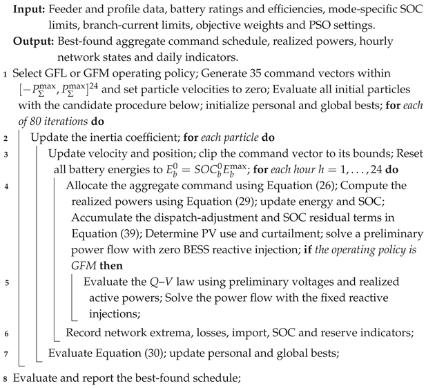 |
2.8. Aggregated Frequency Response Screening
A simplified aggregated frequency model is used only to screen the direction and relative severity of the response following islanding. It assumes a coherent single-frequency state, constant aggregate inertia and damping, and an ideal saturated droop response. It does not represent converter inner current and voltage loops, phase-locked-loop dynamics, virtual impedance, dc-link dynamics, measurement and actuation delays, phase unbalance, harmonic behavior, current-priority logic, protection actions, or interactions among spatially separated inverters. Consequently, the model cannot establish small-signal or transient stability margins, predict fault behavior, or validate the absolute frequency trajectory of a physical inverter. RMS, electromagnetic-transient, controller-hardware-in-the-loop, or power-hardware-in-the-loop studies are required before drawing implementation-level conclusions.
The normalized frequency deviation is modeled as
where is the per unit frequency deviation, H is the virtual inertia time constant, is the active power control response of the grid-forming BESS in per unit, is the active power imbalance after islanding in per unit, D is the aggregated damping coefficient, and t is time in seconds. The frequency is recovered from
where is the system frequency in hertz, and is the nominal frequency, equal to 60 Hz. The grid forming droop response is represented as
where is the frequency droop coefficient, and is the available active power reserve of the BESS. For the grid-following case, is set to zero because this representation does not establish the local frequency reference after islanding.
The screening is applied at hours 12, 18, 19, and 20 using the corresponding pre-islanding grid import and BESS operating point. These hours represent solar production, the evening ramp, and high-import conditions. For each trajectory, the integration is terminated at the first sample below 57 Hz, which is treated as underfrequency loss of service. The reported crossing time is therefore a screening metric; post-threshold dynamics and settling are not inferred.
The application boundary is an aggregated screening of the immediate active-power imbalance after separation and the idealized response associated with the assigned reserve. The model uses kVA, Hz, s, , and , with a 0.005-s integration step and separation at s. The inertia and damping are prescribed aggregate parameters, not identified dynamic properties of the individual converters. A single frequency state is imposed even for the GFL screening case; this construction does not demonstrate that an actual all-GFL island can establish a frequency reference. Accordingly, the model cannot validate transient stability, protection coordination, or the physical accuracy of a frequency nadir or threshold-crossing time.
2.9. Performance Indicators
The daily indicators used in the comparison include imported grid energy, active-energy losses, operating cost, grid-associated emissions, minimum voltage, maximum voltage, maximum branch loading, voltage violation hours, current violation hours, and BESS final SOC deviation. The loss reduction is calculated as
where is the percentage loss reduction, is the daily loss energy in the base case, and is the daily loss energy in the evaluated case. The grid-associated emissions are computed as
where is the daily emitted carbon dioxide mass associated with grid imports, and is the grid emission factor in kgCO2/kWh.
3. Results and Discussion
3.1. Description of the Evaluated Operating Cases
The proposed grid-forming operation strategy was evaluated using 33-bus radial distribution system [38]. The PV generation units were located at buses 13, 25, and 30, with a rated capacity of 800 kW per unit, resulting in an aggregated installed PV capacity of 2.4 MW. The BESS units were placed at buses 6, 14, and 31, with rated active power capacities of 400 kW, 300 kW, and 300 kW, respectively. Their corresponding energy capacities were 1200 kWh, 900 kWh, and 900 kWh.
Figure 2 shows the 33-bus radial distribution network used in this study and identifies the location of the distributed energy resources.
Figure 2.
33-bus radial distribution network for the test system.
Four operating cases were analyzed. The first case corresponds to the base feeder without distributed energy resources. The second case includes PV generation under a grid-following representation. The third case includes PV generation and BESS units operating under grid-following control, where the BESS is represented as an active-power-controllable resource. The fourth case includes PV generation and BESS units operating in grid-forming mode, where the BESS contributes to active-power scheduling and voltage support through reactive power regulation. The daily load demand was 72.915 MWh, while the available PV energy was 10.627 MWh, which represents 14.57% of the daily load demand. Figure 3 presents the hourly demand and PV availability [39].
Figure 3.
Hourly load demand and available photovoltaic generation profiles used in the 33-bus test system.
3.2. Daily Energy, Losses, Cost, and Emissions
Table 7 summarizes the daily performance indicators obtained for the four operating cases. In the base case, the feeder imported 76.294 MWh from the upstream grid and presented daily active-energy losses of 3.379 MWh. The PV-only case reduced the grid import to 64.926 MWh and the daily losses to 2.638 MWh, which corresponds to a loss reduction of 21.94% with respect to the base case. This result confirms that local PV generation reduces the upstream power transfer during the solar availability window.
Table 7.
Daily performance summary for the evaluated operating cases.
The grid-following BESS case did not improve the loss performance obtained with PV generation alone. Its daily losses were 2.778 MWh, equivalent to a 17.79% reduction relative to the base case, but higher than the 2.638 MWh observed in the PV-only case. This behavior indicates that an active-power BESS dispatch, when represented without voltage forming support, can increase feeder currents during charging and discharging intervals. The resulting operation also produced one voltage violation hour, with a minimum voltage of 0.8955 p.u.
The grid-forming BESS case achieved the best daily result in terms of feeder losses, cost, and emissions. The total daily losses decreased to 1.738 MWh, corresponding to a 48.58% reduction with respect to the base case. Compared with the grid-following BESS case, the grid-forming case reduced the daily losses by 37.44%. The same case also produced the lowest operating cost, 6894.98 USD, and the lowest grid-associated emissions, 8067.25 kgCO2. These values represent reductions of 16.74% and 16.08%, respectively, with respect to the base case. Compared with the grid-following BESS case, the cost and emissions decreased by 2.29% and 2.26%, respectively.
Although the grid-forming case produced the highest maximum branch loading (81.70%), no current violations were observed. This result shows that the grid-forming strategy improved the energetic performance of the feeder while preserving the thermal feasibility of the network. However, the branch loading margin was reduced with respect to the base and PV-only cases, which indicates that current constraints should be explicitly considered when grid-forming reactive support is coordinated with active-power scheduling.
3.3. Hourly Behavior of Losses, Voltage, and Grid Power Exchange
Figure 4 compares the hourly active power losses. The base case reached its maximum loss at hour 20, with 191.50 kW. The same peak loss was observed in the PV-only case because PV generation was not available during the evening peak. In contrast, the two PV–BESS cases modified the time of the most stressed operating condition. The grid-following BESS case reached 240.09 kW at hour 18, while the grid-forming BESS case reached 233.23 kW at the same hour. Nevertheless, the average hourly loss was lowest in the grid-forming case at 72.40 kW, followed by the PV-only case at 109.90 kW, the grid-following BESS case at 115.74 kW, and the base case at 140.79 kW.
Figure 4.
Hourly active power loss comparison among the base, PV-only, PV–BESS grid-following, and PV–BESS grid-forming cases.
Figure 5 presents the hourly minimum voltage. The weakest operating condition in the base and PV-only cases occurred at hour 20, with a minimum voltage of 0.9084 p.u. In the PV–BESS cases, the lowest voltage occurred at hour 18. The grid-following BESS case reached 0.8955 p.u., which produced one voltage violation hour. The grid-forming BESS case increased the minimum value at the same stressed interval to 0.9042 p.u., avoiding voltage violations under the adopted operating limits. In addition, the average hourly minimum voltage increased to 0.9568 p.u. in the grid-forming case, compared with 0.9225 p.u. in the base case, 0.9338 p.u. in the PV-only case, and 0.9331 p.u. in the grid-following BESS case.
Figure 5.
Hourly minimum voltage comparison for the evaluated operating cases.
The grid power exchange shown in Figure 6 confirms that the PV-only case reduces upstream imports during the solar window, reaching a minimum grid import of 2098.83 kW at hour 12. The grid-following BESS case reached the lowest hourly import, 1658.56 kW, at hour 10, but it also increased the evening grid import to 4174.52 kW at hour 18. The grid-forming case reached a maximum import of 4412.75 kW at hour 18 due to the coordinated charging action observed in the BESS schedule. Despite this instantaneous increase, its daily grid import was the lowest among all cases, 64.026 MWh. This contrast is explained by the fact that the grid-forming case uses less active-energy throughput over the day and compensates feeder voltage through reactive support, which reduces network losses over multiple hours.
Figure 6.
Slack bus active power exchange for the evaluated operating cases.
3.4. Sensitivity to Load and PV Conditions
The dependence on the daily operating condition is evaluated with three profile combinations: high load/low PV , nominal , and low load/high PV . The optimized BESS schedules and controller settings are held fixed across these cases to measure their operating robustness without masking profile sensitivity through rescheduling. Table 8 compares the two BESS representations. The GFM case retains lower losses, lower cost, and a higher minimum voltage than the GFL case under all three combinations. Relative to GFL, its losses are 35.3%, 37.4%, and 39.3% lower under high-load/low-PV, nominal, and low-load/high-PV conditions, respectively. No current violation or PV curtailment occurs in any of these BESS cases.
Table 8.
Performance under scaled load and PV profiles with fixed BESS schedules.
These scenarios assess sensitivity to operating levels while preserving the hourly shapes of the demand and PV profiles. The load multiplier applies to both active and reactive demand, preserving the load power factor. The BESS command schedules and controller settings are fixed, while the network voltages and voltage-dependent reactive injections are evaluated for each scenario. Relative to GFL, GFM losses are lower by 35.3%, 37.4%, and 39.3% for the high-load/low-PV, nominal, and low-load/high-PV conditions, respectively. Nevertheless, the high-load/low-PV condition gives a GFM minimum voltage of 0.8940 p.u. and one voltage-violation hour, compared with 0.8852 p.u. and two violation hours for GFL. GFM also has higher maximum branch loading in all three conditions. Thus, the observed advantages in losses and selected voltage indicators neither establish universal feasibility nor imply superiority across all operational metrics. Uniform scaling does not reproduce subhourly irradiance fluctuations, altered daily shapes, seasonal variability, or a probability distribution of forecast errors. The conclusions are restricted to the evaluated scenarios and mode-specific operating policies.
3.5. BESS Operation Under Grid-Following and Grid-Forming Modes
Table 9 reports the main BESS operation indicators. The grid-following BESS case showed a larger daily energy throughput, with 3.937 MWh discharged and 4.376 MWh charged. Its final mean state-of-charge was 0.5044, with a final deviation of 0.0076 with respect to the target value. This behavior indicates accurate daily SOC restoration, but the active-power schedule produced higher feeder currents in several intervals and one voltage violation.
Table 9.
BESS operation indicators under grid-following and grid-forming modes.
The GFL and GFM schedules exchange 8312.261 and 2099.595 kWh of daily AC-side active-energy throughput, respectively, corresponding to and . GFM therefore reduces the throughput-based cycling proxy by 74.74%. This is a quantitative utilization comparison and does not establish a 74.74% reduction in capacity fade or replacement cost. Reactive-power provision can impose converter current and thermal stress that is not represented by this active-energy metric. Furthermore, the terminal SOC values differ between policies, so the schedules should not be interpreted as identical energy-restoration duties.
The aggregated GFM schedule showed a maximum charging power of 1000 kW at hour 18 and a maximum discharging power of 637.00 kW at hour 22. It also supplied reactive-power support throughout the day, with aggregated reactive power between 750.00 kVAr and 1249.99 kVAr.
Figure 7 and Figure 8 show the SOC trajectory and the aggregated active-power schedule. The GFL schedule presents frequent charge and discharge transitions, including charging intervals around hours 7, 13, 18, and 22. The GFM schedule remains close to the initial SOC during most of the day and concentrates its main charging action at hour 18, followed by discharge during the evening interval. The terminal drift in the GFM case follows directly from the asymmetric stored-energy balance. Although the rounded AC-side totals are equal, MWh, the stored-energy change is MWh. Relative to the 3.0 MWh installed capacity, this gives an average SOC reduction of approximately 0.036 p.u., consistent with the decrease from 0.5000 to 0.4642. The optimizer accepts this deviation because terminal restoration is implemented as a finite penalty rather than an equality constraint, while loss, import, cost, smoothness, and reserve terms compete in the same objective. The reported deviation of 0.0621 is the Euclidean norm across the three BESS units, whereas 0.4642 is their final mean SOC. If daily neutrality is required, should be imposed as a hard constraint or enforced using an exact repair operator.
Figure 7.
Average state-of-charge of the BESS units under grid-following and grid-forming operation.
Figure 8.
Aggregated BESS active-power schedule under grid-following and grid-forming operation. Positive values indicate discharge, while negative values indicate charge.
3.6. Voltage Profile and Branch Loading
The weakest bus was bus 18 in all evaluated cases. Table 10 summarizes the voltage behavior at this bus. In the base case, the minimum voltage at bus 18 was 0.9084 p.u., and its mean value over the day was 0.9225 p.u. The PV-only case increased the mean voltage at this bus to 0.9338 p.u. but did not modify the evening minimum because PV power was unavailable at the most stressed hour. The grid-following BESS case increased the maximum voltage and preserved a mean value close to the PV-only case, but its minimum voltage decreased to 0.8955 p.u. The grid-forming BESS case produced the highest mean voltage at bus 18, 0.9578 p.u., and increased the maximum value to 0.9718 p.u. This result confirms the positive effect of grid-forming reactive support on the weakest area of the feeder.
Table 10.
Voltage indicators at the weakest bus of the 33-bus system.
Figure 9 presents the voltage profile at the peak load hour. The base and PV-only cases show the expected voltage drop along the main feeder, with the lowest voltages near the downstream buses. The grid-forming BESS case raises the voltage profile across most buses and keeps the entire feeder within the admissible voltage range. This result is consistent with the daily voltage indicators and shows that the proposed grid-forming operation improves voltage support in radial feeders with distributed PV generation.
Figure 9.
Voltage profile at the peak load hour for the evaluated operating cases.
Table 11 reports the branches with the highest loading in each case. In the base and PV-only cases, the maximum occurred on branch 14, between buses 14 and 15, at hour 20. With BESS operation, the limiting branch shifted one section upstream to branch 13, between buses 13 and 14. This branch supplies the downstream buses 14–18 and directly carries the charging or discharging exchange of the BESS connected at bus 14; the PV unit at bus 13 is located at its sending end. In the GFL case, charging near hour 13 increases the downstream active-power transfer and produces a 77.54% peak. In the GFM case, the maximum occurs at hour 18, when the aggregated BESS charging command reaches 1000 kW and the PV contribution is low. The bus-14 share of that charging demand is added to the downstream load, while the voltage controller simultaneously changes the reactive component of branch current. Reactive support can reduce current on several feeder sections, and hence, daily losses, without guaranteeing a reduction in the local peak current of every branch. Thus, the 81.70% branch-13 maximum is compatible with lower daily losses because the two indicators refer to different spatial and temporal aggregations. The branch remains below its thermal limit, but its reduced margin identifies a location where active-power scheduling, Q–V support, and current limits should be coordinated.
Table 11.
Most loaded branch for each operating case.
The 81.705% GFM maximum occurs on branch 13 at hour 18, during aggregate BESS charging of 1000 kW. Its 32.682-A current is evaluated against the prescribed 40-A limit. Because GFL and GFM have different active-power schedules as well as different reactive injections, this comparison does not isolate a reactive-power-only contribution to the peak. The result is interpreted as the combined effect of charging demand, reactive transfer, and local voltage.
After identifying the most loaded branches in Table 11, Figure 10 compares the maximum loading of all feeder branches. The BESS cases increase the loading of the branches close to buses 13 and 14, while the base and PV-only cases remain below 55% loading across the most stressed branches. The grid-forming case remains below the 100% loading limit, but it operates with a smaller thermal margin than the grid following and PV-only cases.
Figure 10.
Maximum branch loading comparison for the evaluated operating cases.
3.7. Objective-Weight Sensitivity
Table 12 evaluates grouped scaling of the objective coefficients. The performance factor multiplies , while the technical-penalty factor multiplies ; remains unchanged. Five GFM searches use 12 particles and 20 iterations, with factors , , , , and and seeds 601–605, respectively. Each search includes the nominal dispatch as an initial candidate. The unit-factor row is a stochastic search outcome under the nominal weights, not a duplicate of the main dispatch. Its lower objective, versus , shows that the main dispatch is not an established optimum. Because seeds also differ, the results describe joint weight and search sensitivity rather than isolated causal effects of individual coefficients.
Table 12.
GFM objective-weight sensitivity. Factors multiply the nominal coefficients.
The five grouped-weight cases in Table 12 produce GFM losses between 1.650 and 1.738 MWh and mean terminal SOC between 0.3551 and 0.4900. The performance multiplier acts on , while the technical multiplier acts on ; is unchanged. All five cases satisfy the stated voltage and branch-current limits, but terminal restoration is not enforced exactly, and the hour-19 reserve margin remains negative. Because random seeds also differ among the searches, the observed spread represents joint weight and stochastic-search sensitivity. It does not identify the isolated effect of an individual coefficient or demonstrate a monotonic response to its value. The nominal-weight search also finds a lower objective than the principal GFM schedule.
3.8. PSO Convergence and Repeatability
Because PSO is stochastic, convergence was examined through five independent runs for each BESS mode using seeds 101, 202, 303, 404, and 505. Each diagnostic run used 15 particles and 30 iterations, whereas the schedules reported in the main comparison used 35 particles and 80 iterations. Table 13 shows the best objective decreases in every diagnostic run. The average reduction from the first recorded best value to the final best value is 59.63% for GFL and 13.76% for GFM. The final-objective coefficient of variation is 22.37% for GFL and 4.48% for GFM, revealing appreciable seed sensitivity in the GFL search and more concentrated GFM outcomes.
Table 13.
Statistical convergence indicators from five independent PSO runs per BESS mode.
Figure 11 presents the normalized best-objective histories. The median final normalized objective is 0.411 for GFL and 0.860 for GFM. Improvements remain active near iteration 30: the mean improvement over the last ten iterations is 9.46% and 4.96%, respectively, and the mean last significant improvement occurs at iterations 29.2 and 29.6. This behavior supports extending the search beyond 30 iterations. The reported search increases the simultaneous candidate population from 15 to 35 particles and extends the refinement interval to 80 iterations; its resulting objective is lower than the best of the five diagnostic runs for both modes. These checks support the adequacy of the adopted computational budget for the comparative study, but they do not constitute a proof of global optimality.
Figure 11.
Median normalized best-objective histories across five independent PSO runs per BESS mode. Each run is normalized by its first recorded best value before calculating the pointwise median.
3.9. Frequency Response Screening Under Islanding
The aggregated frequency screening was applied at hours 12, 18, 19, and 20 to cover solar production, the evening ramp, and high-import conditions. Figure 12 presents hour 19 in detail. Immediately before separation at that hour, the upstream grid supplied 3.339 MW in the GFL-BESS case and 3.567 MW in the GFM-BESS case. The GFM BESS had 0.928 MW of upward active-power headroom, equal to only 26.0% of its pre-islanding deficit. Each trajectory is therefore truncated at its first sample below the 57-Hz underfrequency threshold; values after that event would require an explicit protection, load-shedding, reconnection, or secondary-restoration model.
Figure 12.
Aggregated frequency screening at hour 19. Each curve is terminated at its first sample below 57 Hz because threshold crossing is treated as loss of service, not as frequency recovery.
Table 14 summarizes the four operating points. The reserve-adequacy ratio is the available GFM upward reserve divided by its pre-islanding deficit. It ranges from 22.7% at hour 18 to 48.6% at hour 12 and remains below unity in every case. Consequently, neither control representation sustains the island above 57 Hz.
Table 14.
Multi-hour aggregated islanding screening.
At hour 12, the GFM trajectory crosses the threshold 40 ms later than the GFL trajectory. At hour 18, both modes cross at 1.035 s, whereas the differences at hours 19 and 20 are 5 ms. For hour 19, the initial ROCOF is approximately Hz/s for GFL and Hz/s for GFM. The larger initial magnitude in the GFM case follows from its larger pre-islanding grid import. No settling time is inferred because each trajectory is terminated at the underfrequency threshold.
Crossing times are measured on the simulation time axis; for example, s corresponds to 35 ms after separation. A 5 ms difference between cases equals one integration step and should not be interpreted as a precisely resolved physical improvement. Moreover, the two operating policies have different pre-islanding grid imports, so their crossing-time differences combine disturbance magnitude and modeled response. Both representations cross the 57-Hz threshold at hours 12, 18, 19, and 20. These results show that the selected screening criterion fails under the adopted assumptions, rather than reflecting experimentally validated islanding performance.
3.10. Main Technical Implications
The obtained results indicate that the value of the BESS in a PV-rich radial distribution network depends strongly on the adopted inverter control representation. When the BESS is modeled as a grid following active-power resource, the feeder benefits are mainly associated with energy shifting. This operation can reduce grid imports during selected hours, but it may increase losses, branch loading, and voltage stress if the charging and discharging schedule is not coordinated with local voltage conditions. In the evaluated case, the grid-following BESS reduced losses by 17.79% relative to the base case but performed worse than the PV-only case in terms of daily losses.
When the BESS is operated as a grid forming resource, the same feeder obtains simultaneous improvements in daily losses, voltage support, cost, and emissions. The daily loss reduction reached 48.58%, while the average hourly minimum voltage increased to 0.9568 p.u. These improvements are explained by the combination of active-power scheduling and reactive-power support, which changes the voltage profile and reduces the current magnitude across several feeder sections. However, the multi-hour screening does not demonstrate successful islanding. Both BESS modes cross the 57-Hz threshold at hours 12, 18, 19, and 20 because the pre-islanding deficit exceeds the available GFM active-power reserve. GFM delays the crossing by 0–40 ms, depending on the operating point. This negative result prevents the steady-state feeder benefits from being interpreted as proof of islanding adequacy.
The results also expose two operational tradeoffs. First, grid forming support increased the maximum branch loading to 81.70%, which remained feasible but reduced the thermal margin. Second, the final SOC deviation in the grid-forming case was larger than in the grid-following case. Future scheduling formulations should impose terminal SOC restoration and explicitly coordinate branch loading and converter current limits with active and reactive support.
Several practical factors remain outside the present simulation boundary. Semiconductor current limits and the associated active/reactive current-priority logic can modify the commanded GFM response during severe voltage deviations. Protection settings that are adequate in grid-connected operation may lose sensitivity or coordination after islanding because inverter fault current is limited and control dependent. In addition, the computational and coordination burden grows with feeder size, the number of controllable converters, phase unbalance, discrete utility devices, and communication constraints. The present balanced 33-bus results therefore require validation on larger and unbalanced feeders, followed by utility-data calibration and staged RMS, EMT, controller-hardware-in-the-loop, or field testing before practical deployment.
4. Conclusions
This study closes a feeder-level research gap in the assessment of BESS inverter representation for PV-rich radial distribution networks. While previous studies have mainly analyzed grid-forming control, BESS scheduling, PV voltage regulation, or islanding behavior separately, this work integrates 24-h BESS scheduling, radial AC power flow, converter apparent-power limits, voltage support, branch loading, cost, emissions, direct GFL/GFM comparison, and islanding screening within the same 33-bus distribution feeder.
Among the four principal operating cases, the GFM BESS representation achieved the lowest daily feeder losses, grid imports, and energy-purchase cost, while exhibiting higher maximum branch loading and greater terminal SOC deviation than the GFL BESS case. Daily active-energy losses decreased from 3.379 MWh in the base case to 1.738 MWh in the GFM BESS case, corresponding to a 48.58% reduction. In contrast, the GFL BESS case reduced losses by 17.79% relative to the base case but performed worse than the PV-only case. The GFM BESS case also reduced daily grid imports to 64.026 MWh, decreased the operating cost to 6894.98 USD, and lowered grid-associated emissions to 8067.25 kgCO2. From a voltage perspective, the GFM BESS case increased the average hourly minimum voltage to 0.9568 p.u. and avoided voltage violations, whereas the GFL BESS case produced one voltage-violation hour.
These findings provide a relevant engineering insight for BESS planning and operation: storage should not be represented only as an active-power scheduling device when its converter can operate in grid-forming mode. The combination of active-power scheduling and voltage-dependent reactive-power support modified the feeder voltage profile and reduced losses over several hours. The ordering of daily losses persists under the three evaluated load/PV combinations, but the high-load/low-PV condition produces a voltage violation even with GFM support. This evidence supports conditional performance across the tested operating levels, not general robustness to renewable uncertainty or arbitrary distribution-network conditions. The multi-hour islanding results did not establish viable islanded operation because active-power reserve remained insufficient.Therefore, BESS control mode selection can affect feeder losses, voltage security, thermal margins, operating cost, emissions, and islanding headroom, even when the installed storage capacity remains unchanged.
The transferable conclusion is qualitative: when active-power scheduling and local voltage-dependent reactive support share a finite converter capability, the BESS control representation can change feeder losses, voltage support, thermal loading, cycling, and islanding headroom. In addition, voltage-support benefits do not by themselves establish adequate active-power reserve for islanding. The reported percentages, limiting buses and branches, critical hours, SOC drift, and frequency metrics are specific to the adopted 33-bus topology, DER placement and ratings, daily profiles, objective weights, and simplified control models. Applying the method to another network requires feeder-specific parameterization, renewed optimization, and validation; it should not be assumed that GFM operation will produce the same numerical gains or remain the best case under every topology and operating condition.
The study also identifies relevant limitations and future research directions. The GFM BESS case increased the maximum branch loading to 81.70% under the nominal condition and to 86.78% under high load and low PV. In addition, the final SOC deviation was higher than in the GFL BESS case, PV inverters were restricted to unity power factor, and the frequency assessment used an aggregated model rather than a detailed dynamic or electromagnetic-transient representation. Future work should include hard terminal SOC restoration, chemistry-specific degradation costs, scenario-based scheduling, PV reactive-power capability, converter current-limiting behavior, optimized GFM control parameters, broader islanding contingencies, and detailed RMS, EMT, or hardware-in-the-loop validation under islanding and fault conditions.
Author Contributions
Conceptualization, D.S.-V.; methodology, D.S.-V., V.B.-G. and A.F.M.P.; software, D.S.-V., V.B.-G. and A.F.M.P.; validation, D.S.-V.; formal analysis, D.S.-V., V.B.-G. and A.F.M.P.; investigation, D.S.-V., V.B.-G. and A.F.M.P.; data curation, V.B.-G. and A.F.M.P.; writing—original draft preparation, D.S.-V., V.B.-G. and A.F.M.P.; writing—review and editing, D.S.-V., V.B.-G. and A.F.M.P.; visualization, D.S.-V., V.B.-G. and A.F.M.P.; supervision, D.S.-V. All authors have read and agreed to the published version of the manuscript.
Funding
This research received no external funding.
Data Availability Statement
Data is contained within the article.
Acknowledgments
During the preparation of this work, the authors used AI-assisted writing tools to improve clarity and language. After using these tools, the authors reviewed and edited the content as needed and take full responsibility for the publication’s content.
Conflicts of Interest
The authors declare no conflicts of interest.
Nomenclature
Symbols and abbreviations used in the manuscript.
| Symbol | Definition |
| Sets, indices and mathematical operators | |
| Set of distribution-network buses. | |
| Set of distribution-network branches. | |
| Set of hourly scheduling intervals, . | |
| Set of buses with PV generation. | |
| Set of BESS connection buses or units. | |
| Bus indices; j also denotes the imaginary unit in complex-valued expressions. | |
| Branch indices. | |
| b | BESS unit index. |
| h | Hourly scheduling index. |
| Sending and receiving buses of branch ℓ. | |
| Connection bus of BESS unit b. | |
| Slack-bus index. | |
| Set of downstream branches leaving bus . | |
| Positive part of z, defined as . | |
| Complex conjugate. | |
| Magnitude of a scalar or cardinality of a set, according to context. | |
| sat | Saturation operator that clips a command to specified bounds. |
| Network, demand, and PV quantities | |
| Branch impedance, resistance, and reactance. | |
| Voltage magnitude and phase angle at bus i and hour h. | |
| Complex bus voltage. | |
| Preliminary voltage magnitude used to evaluate the BESS reactive command. | |
| Lower and upper admissible bus-voltage magnitudes. | |
| Minimum and maximum bus-voltage magnitudes at hour h. | |
| Reported minimum, maximum, and mean voltage indicators; their aggregation domain is specified by the relevant table or figure. | |
| Net complex demand at bus i and hour h. | |
| Complex current associated with the net bus demand. | |
| Branch current; the thermal-loading calculation uses its magnitude in amperes. | |
| Branch current expressed in per unit. | |
| Prescribed maximum admissible branch current. | |
| Branch loading as a percentage of the prescribed current limit. | |
| Maximum branch loading at hour h. | |
| Apparent-power, voltage, and current bases. | |
| Base active and reactive demands at bus i. | |
| Hourly active and reactive bus demands. | |
| Hourly demand multiplier. | |
| Normalized PV generation factor. | |
| Installed PV active-power capacity at bus i. | |
| Available PV active power. | |
| PV active- and reactive-power injections. | |
| Curtailed PV active power. | |
| Active power exchanged with the upstream grid; positive values denote import. | |
| Total feeder active-power loss at hour h. | |
| Battery operation and reactive-power representation | |
| Realized net BESS active power, positive for discharge and negative for charge. | |
| Nonnegative discharging and charging powers. | |
| Battery active- and reactive-power injections at network bus i. | |
| BESS reactive-power injection. | |
| Aggregate BESS active-power command at hour h. | |
| Active-power command allocated to BESS unit b. | |
| Aggregate realized BESS active power. | |
| Rated discharging and charging powers. | |
| Individual and aggregate BESS active-power ratings. | |
| Power scale used to normalize the command-adjustment penalty. | |
| Available discharge and charge power limits considering power ratings and stored energy. | |
| Stored battery energy at the end of hour h and at initialization. | |
| Symbols used for the rated battery energy capacity. | |
| Charging and discharging efficiencies. | |
| Battery state of charge and its initial value. | |
| Admissible lower and upper SOC bounds. | |
| Arithmetic mean of the battery SOC values at hour h. | |
| Mean-SOC target used in the reserve penalty. | |
| Reported mean terminal SOC. | |
| Minimum and maximum SOC attained in the reported BESS trajectories. | |
| Aggregate daily charged and discharged energies. | |
| Sum of daily AC-side charged and discharged energies. | |
| Throughput-based equivalent-full-cycle proxy. | |
| Reported maximum aggregate charging and discharging powers. | |
| BESS converter apparent-power rating. | |
| Available reactive-power magnitude at the realized active-power operating point. | |
| Saturated voltage-dependent reactive-power command. | |
| Voltage reference and voltage deviation associated with full reactive capability. | |
| Aggregate BESS reactive power in the reactive-energy indicator. | |
| Reported extrema of aggregate BESS reactive power. | |
| Objective function and performance indicators | |
| Vector of 24 aggregate BESS active-power commands. | |
| J | Scalar objective value minimized by PSO. |
| Daily feeder loss energy, imported grid energy, and curtailed PV energy. | |
| Loss energies for the reference base case and evaluated case. | |
| Percentage reduction in loss energy relative to the selected base case. | |
| Daily grid-energy purchase cost. | |
| Hourly energy price and its prescribed multiplier. | |
| Grid-associated emissions and the grid-emission factor. | |
| Weights for losses, imported energy, energy-purchase cost, and curtailment. | |
| Weights for voltage, current, SOC/command adjustment, terminal restoration, smoothness and reserve penalties. | |
| Penalties for hourly voltage and branch-loading violations. | |
| Penalty for battery command adjustment and residual SOC-bound violations. | |
| Terminal SOC restoration and command-smoothness penalties. | |
| GFM reserve-shortfall and mean-SOC penalty. | |
| Hourly available reserve indicator and required reserve, expressed in kW. | |
| Aggregated frequency screening | |
| Simulation time and time of separation from the upstream grid. | |
| Scheduling time step, equal to one hour. | |
| Per-unit frequency deviation; distinct from the scheduling vector . | |
| Screened frequency and nominal frequency. | |
| H | Prescribed aggregate inertia time constant. |
| D | Prescribed aggregate damping coefficient. |
| Frequency-droop coefficient. | |
| Idealized active-power control response in per unit. | |
| Active-power imbalance following separation, in per unit. | |
| Reserve magnitude used in the frequency model, in per unit. | |
| Abbreviations | |
| AC, DC | Alternating current; direct current. |
| BESS | Battery energy storage system. |
| DER | Distributed energy resource. |
| EFC | Equivalent full cycle. |
| EMT | Electromagnetic transient. |
| GFL, GFM | Grid-following; grid-forming. |
| HIL | Hardware in the loop. |
| HVDC | High-voltage direct current. |
| IBR | Inverter-based resource. |
| PSO | Particle swarm optimization. |
| PV | Photovoltaic. |
| RMS | Root mean square. |
| RMSE | Root mean square error. |
| ROCOF | Rate of change of frequency. |
| SOC | State of charge. |
| CV | Coefficient of variation. |
| p.u. | Per unit. |
| UF | Underfrequency. |
References
- Rajesh, M.; Ouassaid, M. Impacts of High Renewable Energy Penetration in Low Voltage Distribution Network: A Review. IFAC-PapersOnLine 2024, 58, 636–643. [Google Scholar] [CrossRef] [Scilit]
- Diahovchenko, I.; Morva, G.; Chuprun, A.; Keane, A. Comparison of Voltage Rise Mitigation Strategies for Distribution Networks with High Photovoltaic Penetration. Renew. Sustain. Energy Rev. 2025, 212, 115399. [Google Scholar] [CrossRef] [Scilit]
- Angkasa, F.F.; Givisiez, A.G.; Liu, M.Z.; Ochoa, L.F.; Gutierrez-Lagos, L.; Kaloudas, C.G. Designing Future Residential LV Networks with EVs and PVs: A Bi-Period OPF-Based Approach. Electr. Power Syst. Res. 2026, 250, 112109. [Google Scholar] [CrossRef] [Scilit]
- Astapov, V.; Shabbir, N.; Rosin, A.; Kütt, L.; Maask, V.; Tiismus, H. Review of Technical Solutions Addressing Voltage and Operational Challenges in a Distribution Grid with High Penetration of Intermittent RES. Energy Rep. 2025, 14, 1738–1760. [Google Scholar] [CrossRef] [Scilit]
- Bahrani, B.; Ravanji, M.H.; Kroposki, B.; Ramasubramanian, D.; Guillaud, X.; Prevost, T.; Cutululis, N.A. Grid-Forming Inverter-Based Resource Research Landscape: Understanding the Key Assets for Renewable-Rich Power Systems. IEEE Power Energy Mag. 2024, 22, 18–29. [Google Scholar] [CrossRef] [Scilit]
- Jaradat, T.; Khatib, T. A Review of Battery Energy Storage System for Renewable Energy Penetration in Electrical Power System: Environmental Impact, Sizing Methods, Market Features, and Policy Frameworks. Future Batter. 2025, 7, 100106. [Google Scholar] [CrossRef] [Scilit]
- Inaolaji, A.; Wu, D.; Kopsidas, K. Optimal Allocation of Battery Energy Storage Systems for Peak Shaving and Reliability Enhancement in Distribution Systems. J. Energy Storage 2024, 86, 111327. [Google Scholar] [CrossRef] [Scilit]
- Licari, J.; Rhaili, S.E.; Micallef, A.; Spiteri Staines, C. Addressing Voltage Regulation Challenges in Low Voltage Distribution Networks with High Renewable Energy and Electrical Vehicles: A Critical Review. Energy Rep. 2025, 14, 2977–2997. [Google Scholar] [CrossRef] [Scilit]
- Klink, J.; Helm, S.; Yang, W.; Deblon, F.; Benger, R.; Hauer, I.; Lindemann, A. Instantaneous Reserve by Battery Energy Storage Systems: A Holistic System Model to Analyze the Dynamic Power System Interactions. Energy Rep. 2025, 13, 3096–3111. [Google Scholar] [CrossRef] [Scilit]
- Sakib, S.; Hossain, M.B.; Zamee, M.A.; Hossain, M.J.; Habib, M.A. Role of Battery Energy Storage Systems: A Review on Renewable Energy Zones Integration in Weak Transmission Networks. J. Energy Storage 2025, 128, 117223. [Google Scholar] [CrossRef] [Scilit]
- Ramasubramanian, D.; Kroposki, B.; Dhople, S.; Gros, D.; Hoke, A.; Wang, W.; Shah, S.; Hart, P.; Seo, G.S.; Ropp, M.; et al. Performance Specifications for Grid-Forming Technologies. In Proceedings of the 2023 IEEE Power & Energy Society General Meeting, Orlando, FL, USA, 16–20 July 2023; pp. 1–5. [Google Scholar] [CrossRef] [Scilit]
- Shah, S.; Yan, W.; Koralewicz, P.; Gevorgian, V.; Hoke, A.; Ropp, M.; Kroposki, B.; Seo, G.S.; Ramasubramanian, D. A Testing Framework for Grid-Forming Resources. In Proceedings of the 2023 IEEE Power & Energy Society General Meeting, Orlando, FL, USA, 16–20 July 2023; pp. 1–5. [Google Scholar] [CrossRef] [Scilit]
- Mohammed, N.; Udawatte, H.; Zhou, W.; Hill, D.J.; Bahrani, B. Grid-Forming Inverters: A Comparative Study of Different Control Strategies in Frequency and Time Domains. IEEE Open J. Ind. Electron. Soc. 2024, 5, 185–214. [Google Scholar] [CrossRef] [Scilit]
- Jiang, S.; Zhu, Y.; Xu, T.; Konstantinou, G. Current-Synchronization Control of Grid-Forming Converters for Fault Current Limiting and Enhanced Synchronization Stability. IEEE Trans. Power Electron. 2024, 39, 5271–5285. [Google Scholar] [CrossRef] [Scilit]
- Jiang, S.; Zhu, Y.; Konstantinou, G. Bandwise Power-Synchronization Loop for Frequency Response Improvement in Grid-Forming Converters. IEEE Trans. Power Electron. 2024, 39, 10693–10698. [Google Scholar] [CrossRef] [Scilit]
- Jiang, S.; Zhu, Y.; Xu, T.; Konstantinou, G. Frequency Domain Inertia Design of Grid-Forming Converters. IEEE Trans. Power Electron. 2025, 40, 8886–8898. [Google Scholar] [CrossRef] [Scilit]
- Han, F.; Zhang, X.; Li, M.; Li, F.; Zhao, W. Stability Control for Grid-Connected Inverters Based on Hybrid-Mode of Grid-Following and Grid-Forming. IEEE Trans. Ind. Electron. 2024, 71, 10750–10760. [Google Scholar] [CrossRef] [Scilit]
- Safamehr, H.; Izadi, I.; Ghaisari, J. Robust V-I Droop Control of Grid-Forming Inverters in the Presence of Feeder Impedance Variations and Nonlinear Loads. IEEE Trans. Ind. Electron. 2024, 71, 504–512. [Google Scholar] [CrossRef] [Scilit]
- Ai, C.; Li, Y.; Zhao, Z.; Gu, Y.; Liu, J. An Extension of Grid-Forming: A Frequency-Following Voltage-Forming Inverter. IEEE Trans. Power Electron. 2024, 39, 12118–12123. [Google Scholar] [CrossRef] [Scilit]
- Chen, Y.; Zheng, K.; Feng, C.; Huang, J.; Guo, H.; Zhong, H. Optimal Grid-Forming BESS Management Incorporating Internal Battery Physics. Appl. Energy 2025, 385, 125448. [Google Scholar] [CrossRef] [Scilit]
- Chen, X.; Huang, Z.; Yin, X.; Liang, Z. Control Damping Enhancement Method of Grid-Forming Battery Energy Storage System with Diverse Synchronization Controls in Asymmetrical Grids. J. Energy Storage 2025, 133, 118028. [Google Scholar] [CrossRef] [Scilit]
- Li, L.; Song, H.; Yan, Z.; Li, H.; Jin, P.; Zhao, J.; Qi, C. A Two-Stage Robust Optimization Strategy for Microgrids Considering the Grid-Forming Capability of Energy Storage and Uncertainties of Wind, Photovoltaic, and Load. J. Energy Storage 2025, 140, 118841. [Google Scholar] [CrossRef] [Scilit]
- Liyanage, C.; Meegahapola, L.; Nutkani, I.; Jalili, M. A Techno-Economic Optimisation Framework for Grid-Forming Battery Inverter Sizing in Renewable Dominant Power Grids. J. Energy Storage 2026, 144, 119704. [Google Scholar] [CrossRef] [Scilit]
- Tang, W.; Huang, Y.; Qian, T.; Wei, C.; Wu, J. Coordinated Central-Local Control Strategy for Voltage Management in PV-Integrated Distribution Networks Considering Energy Storage Degradation. Appl. Energy 2025, 389, 125684. [Google Scholar] [CrossRef] [Scilit]
- Hossain, M.K.; Chowdhury, P.; Nowshin, I.; Islam, M.R.; Al-Hysam, A.; Farrok, O. Grid-connected inverter for photovoltaic energy harvesting: Advances in topologies and control techniques. Energy Convers. Manag. X 2026, 29, 101422. [Google Scholar] [CrossRef] [Scilit]
- Tawfiq, K.B.; Zeineldin, H.; Al-Durra, A.; El-Sadaany, E.F. Enhancing photovoltaic grid integration with hybrid energy storage and a novel three-phase ten-switch inverter for superior power quality. Int. J. Electr. Power Energy Syst. 2025, 167, 110580. [Google Scholar] [CrossRef] [Scilit]
- Khan, M.K.; Kauhaniemi, K.; Laaksonen, H.; Hassan, M.A. Review of recent developments in grid codes: Focus on compliance testing and grid-forming inverter-based resources. Renew. Sustain. Energy Rev. 2026, 227, 116509. [Google Scholar] [CrossRef] [Scilit]
- Ghadiriyan, S.; Rahimi, M. Grid-Forming Assisted Based Power Management of AC Microgrid System Comprising Multiple Battery Energy Storage Units, DFIG-Based Wind Turbines and Inverter-Based Resources. J. Energy Storage 2024, 97, 112772. [Google Scholar] [CrossRef] [Scilit]
- Tafizare, E.; Rahimi, M. Grid-Following and Grid-Forming Control Modes of the Rotor and Grid Sides Converters for Seamless and Universal Operation of the Hybrid DFIG-Wind/Battery Energy Storage System in Grid-Connected and Stand-Alone Conditions. J. Energy Storage 2024, 104, 114623. [Google Scholar] [CrossRef] [Scilit]
- Syahbani, M.A.; Ramli, M.A.M.; Megantoro, P.; Ardiansyah, A.; Cahyani, I.D.; Dinata, N.F.P.; Firmansyah, R.; Zohri, M.; Budiman, F.N. Performance Enhancement of Grid-Forming Inverter-Controlled PV Systems: A Comparative Study with and without Battery Energy Storage under Intermittent and Unbalanced Load Conditions. Results Eng. 2025, 27, 105980. [Google Scholar] [CrossRef] [Scilit]
- Sakib, S.; Hossain, M.J. Severity-Aware Coordination of Grid-Forming and Grid-Following BESS for Stability Enhancement in Weak Transmission Networks. Electr. Power Syst. Res. 2026, 254, 112658. [Google Scholar] [CrossRef] [Scilit]
- Baeckeland, N.; Chatterjee, D.; Lu, M.; Johnson, B.; Seo, G.S. Overcurrent Limiting in Grid-Forming Inverters: A Comprehensive Review and Discussion. IEEE Trans. Power Electron. 2024, 39, 14493–14517. [Google Scholar] [CrossRef] [Scilit]
- Reno, M.J.; Brahma, S.; Bidram, A.; Ropp, M.E. Influence of Inverter-Based Resources on Microgrid Protection: Part 1: Microgrids in Radial Distribution Systems. IEEE Power Energy Mag. 2021, 19, 36–46. [Google Scholar] [CrossRef] [Scilit]
- Faheem, M.; Gungor, V.C. Capacity and Spectrum-Aware Communication Framework for Wireless Sensor Network-Based Smart Grid Applications. Comput. Stand. Interfaces 2017, 53, 48–58. [Google Scholar] [CrossRef] [Scilit]
- Xu, R.; Jiang, Q.; Li, B.; Liu, Y.; Zhu, Y.; Gu, Y.; Liu, T. Frequency-Spectra Impedance Margin Ratio for Stability Analysis of IBR-Penetrated Systems. IEEE Trans. Power Syst. 2026, 1–16. [Google Scholar] [CrossRef] [Scilit]
- Gerini, F.; Zuo, Y.; Gupta, R.; Zecchino, A.; Yuan, Z.; Vagnoni, E.; Cherkaoui, R.; Paolone, M. Optimal grid-forming control of battery energy storage systems providing multiple services: Modeling and experimental validation. Electr. Power Syst. Res. 2022, 212, 108567. [Google Scholar] [CrossRef] [Scilit]
- Kennedy, J.; Eberhart, R. Particle Swarm Optimization. In Proceedings of the ICNN’95—International Conference on Neural Networks, Perth, Australia, 27 November–1 December 1995; Volume 4, pp. 1942–1948. [Google Scholar] [CrossRef] [Scilit]
- Figueroa-Saavedra, H.A.; Sanin-Villa, D.; Grisales-Noreña, L.F. A Tuned Parallel Population-Based Genetic Algorithm for BESS Operation in AC Microgrids: Minimizing Operational Costs, Power Losses, and Carbon Footprint in Grid-Connected and Islanded Topologies. Electricity 2025, 6, 45. [Google Scholar] [CrossRef] [Scilit]
- Sanin-Villa, D.; Figueroa-Saavedra, H.A.; Grisales-Noreña, L.F. Efficient BESS Scheduling in AC Microgrids via Multiverse Optimizer: A Grid-Dependent and Self-Powered Strategy to Minimize Power Losses and CO2 Footprint. Appl. Syst. Innov. 2025, 8, 85. [Google Scholar] [CrossRef] [Scilit]
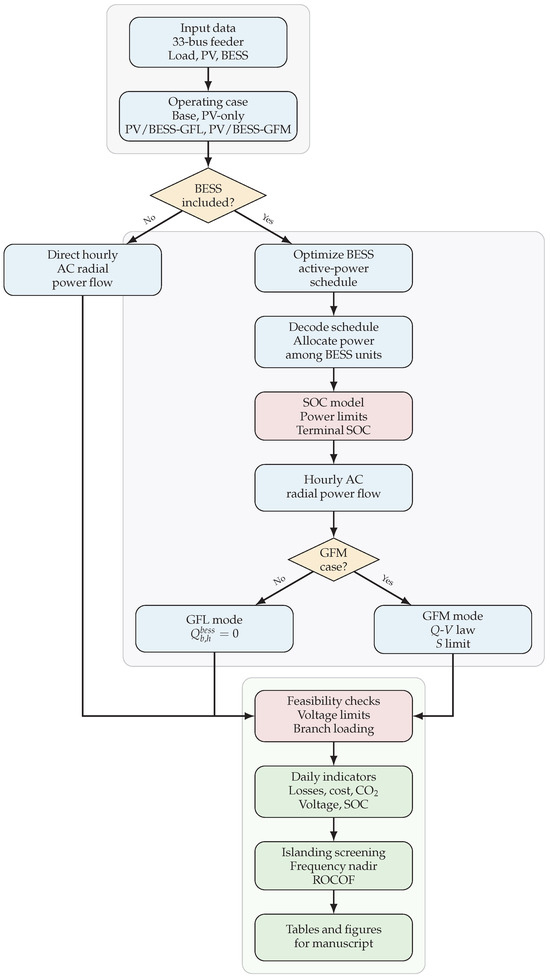
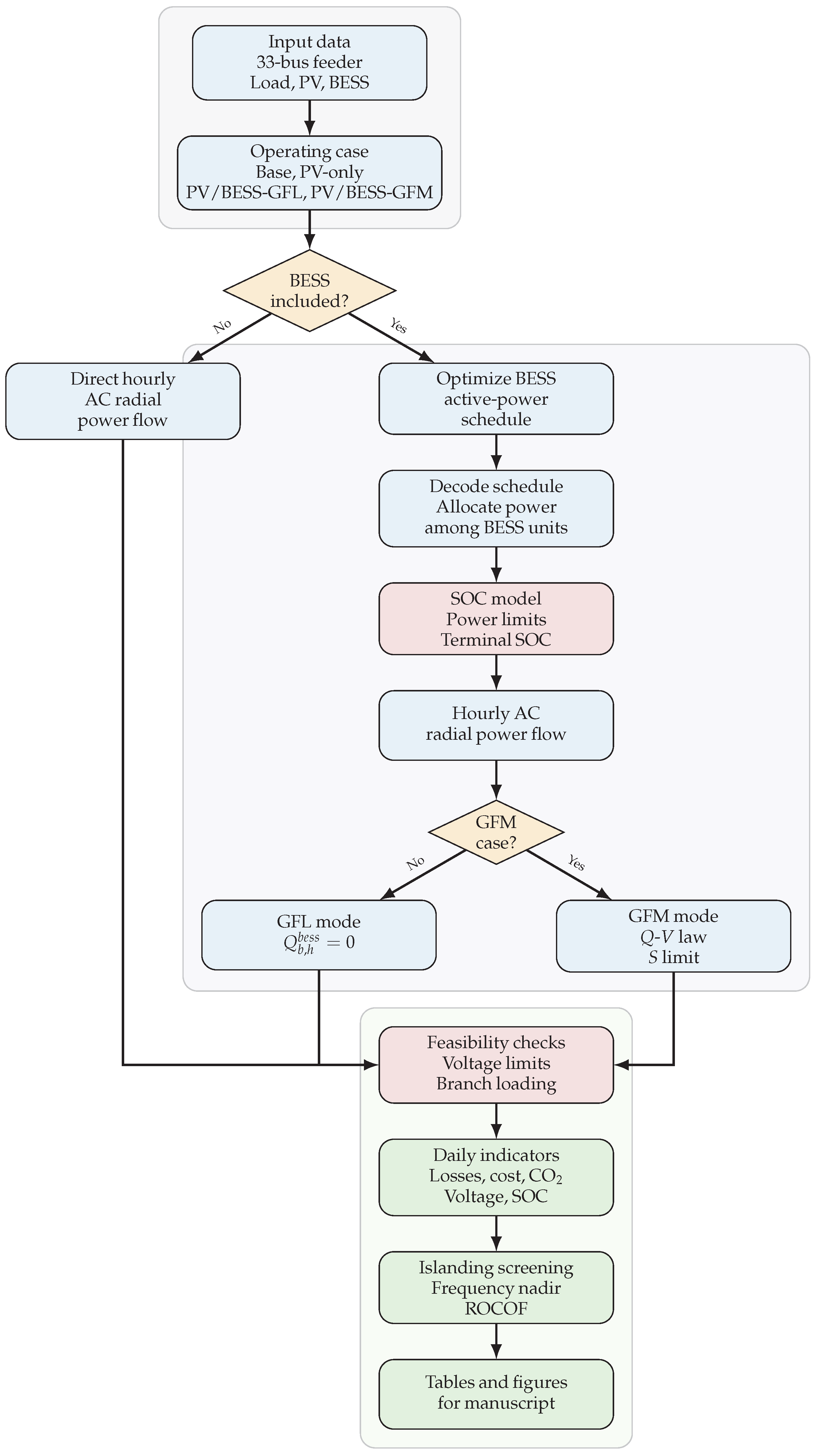
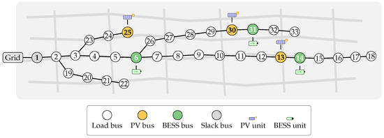
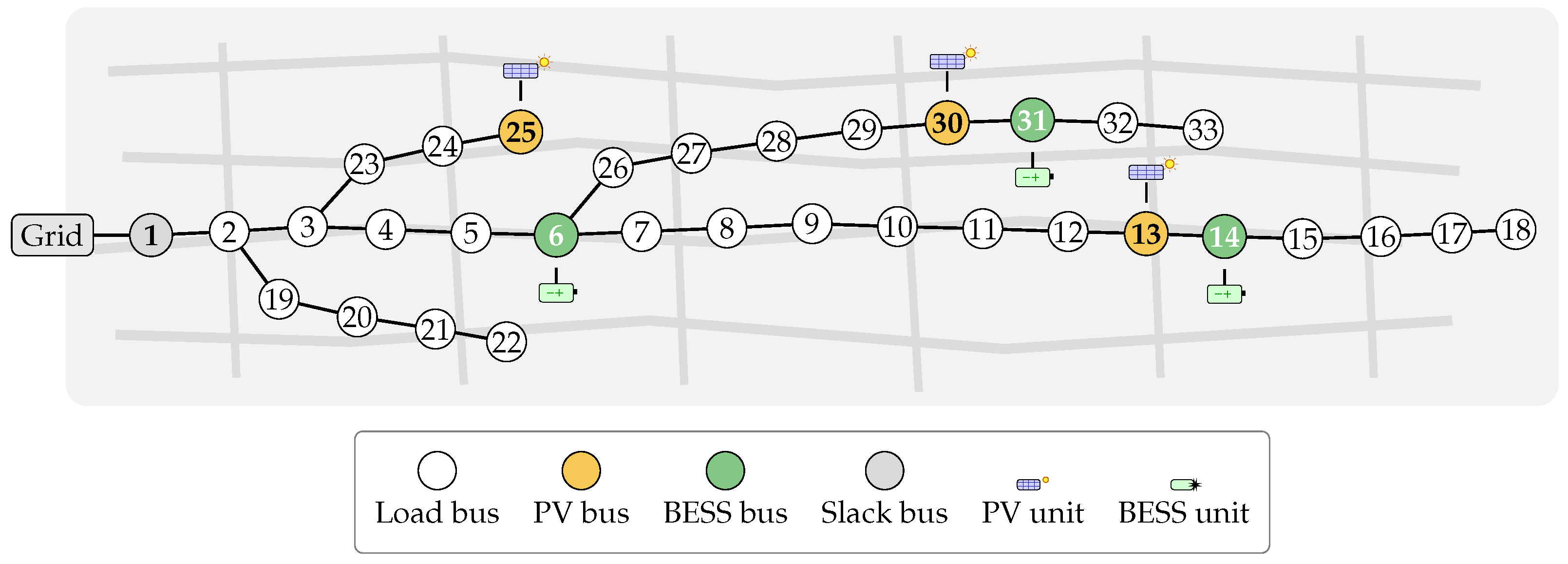
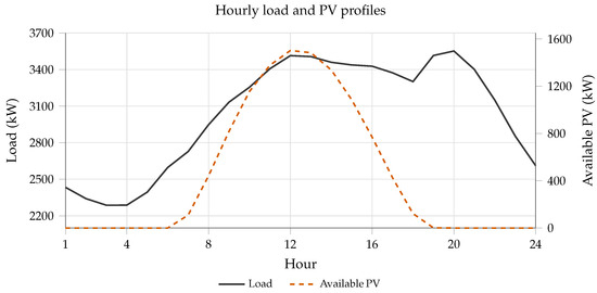
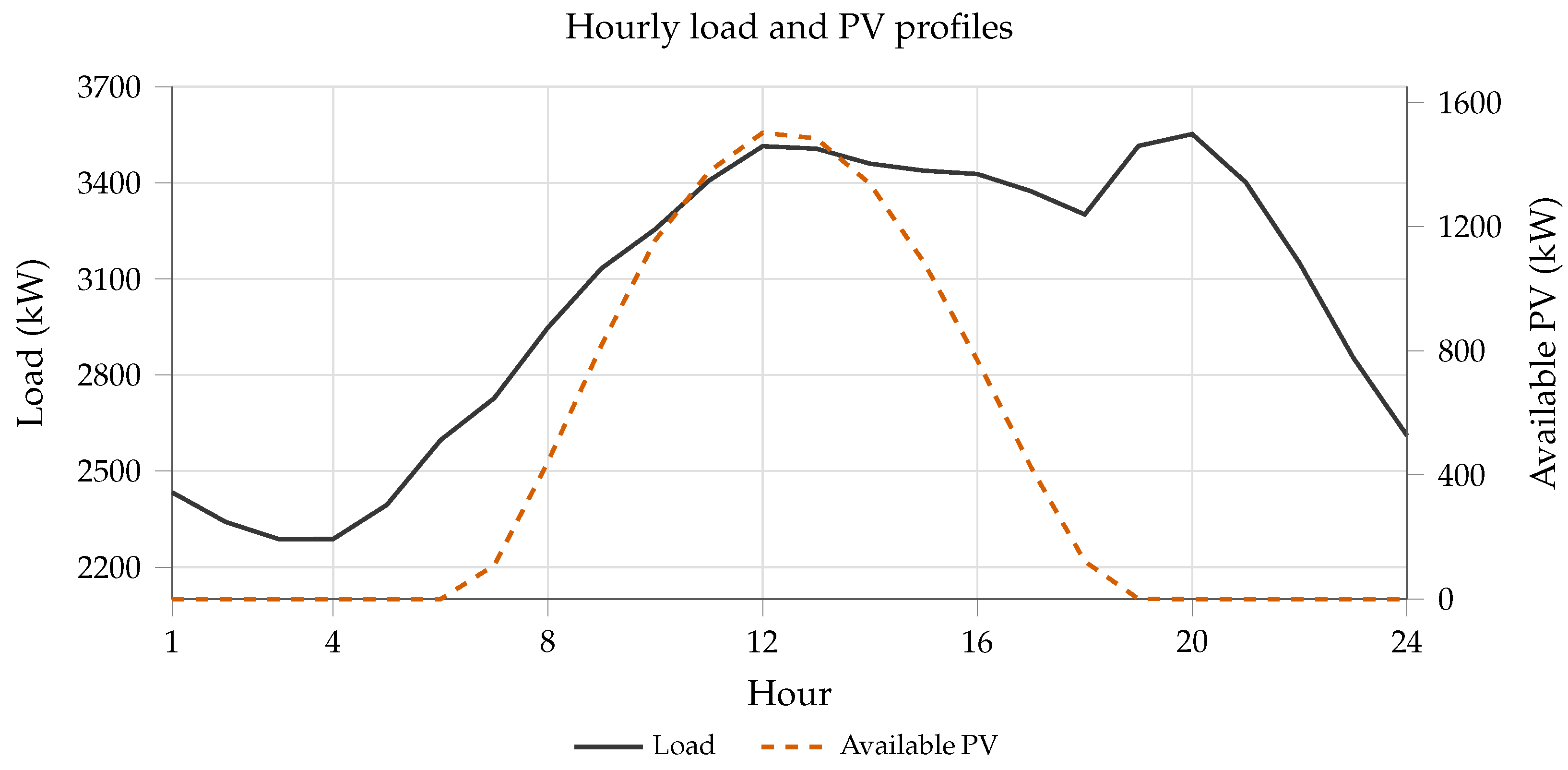
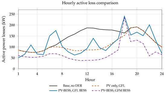
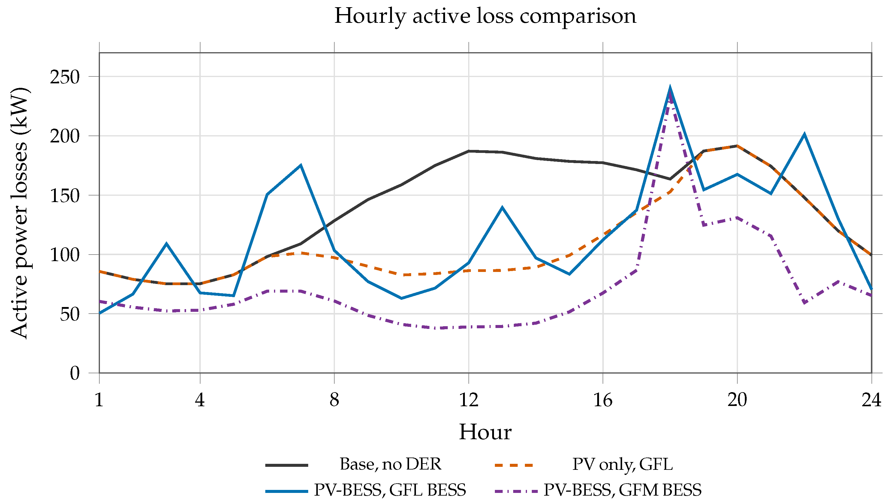
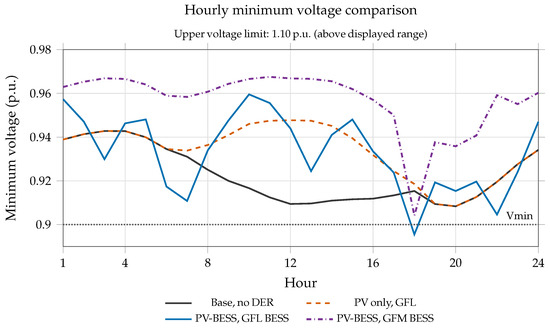
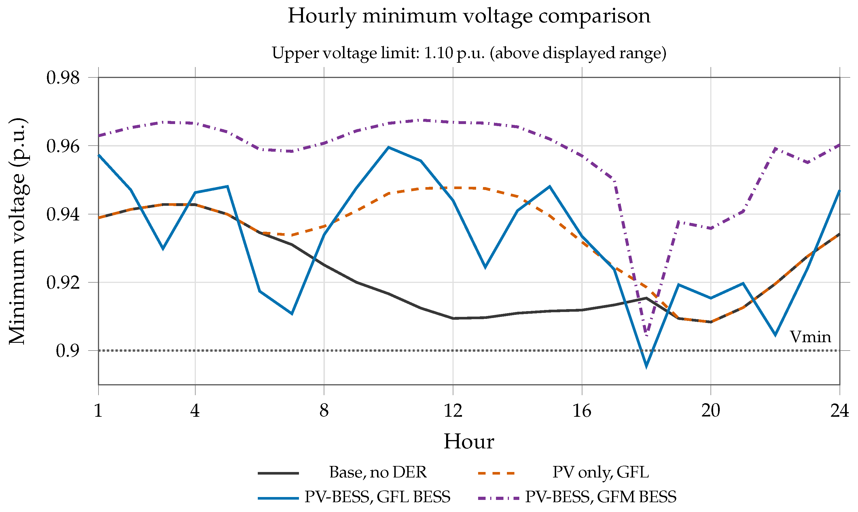
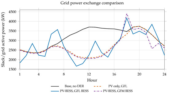
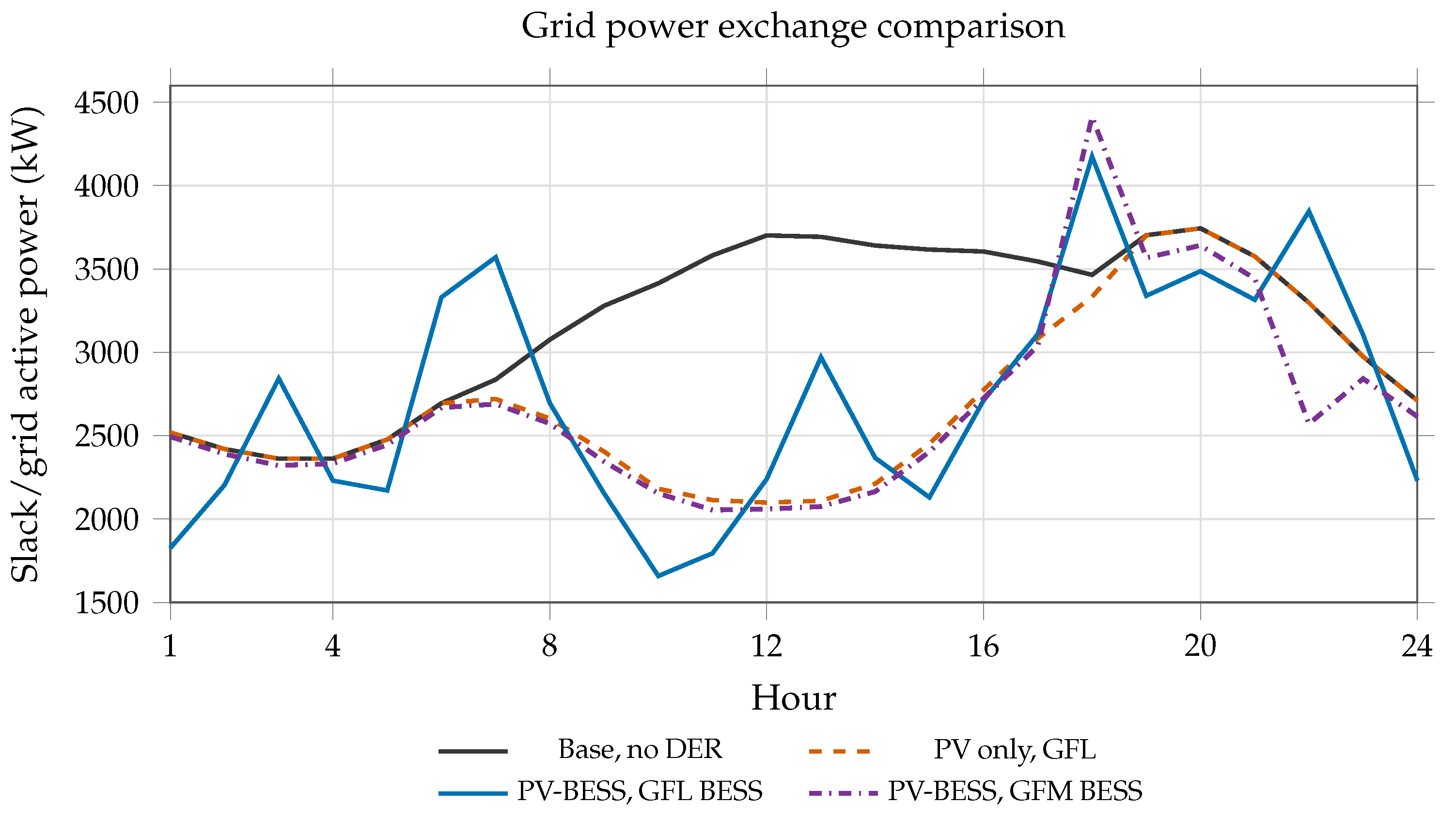
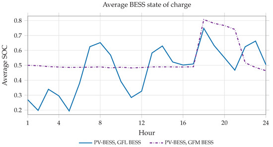
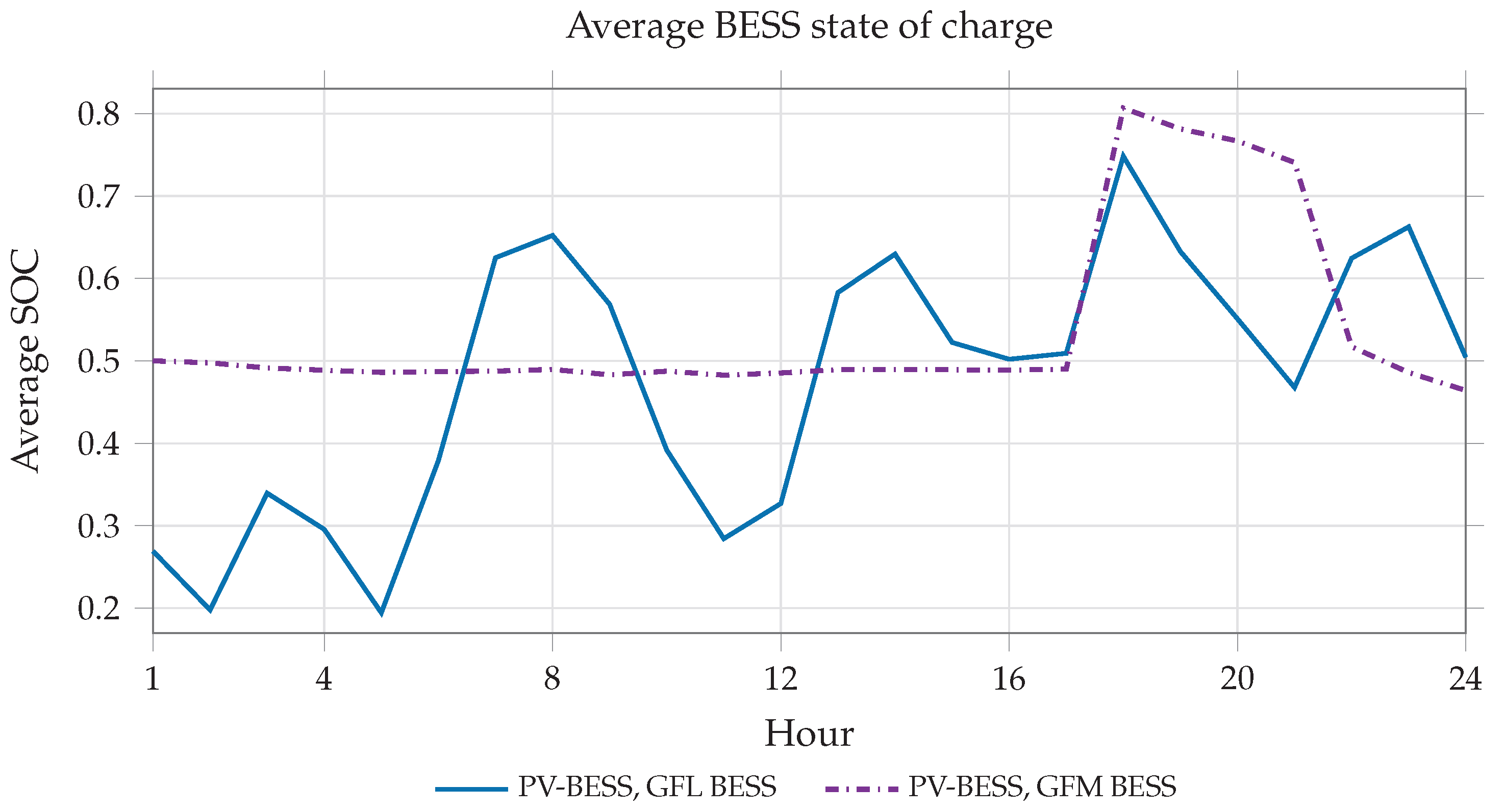
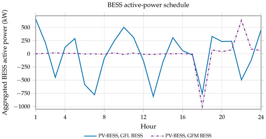
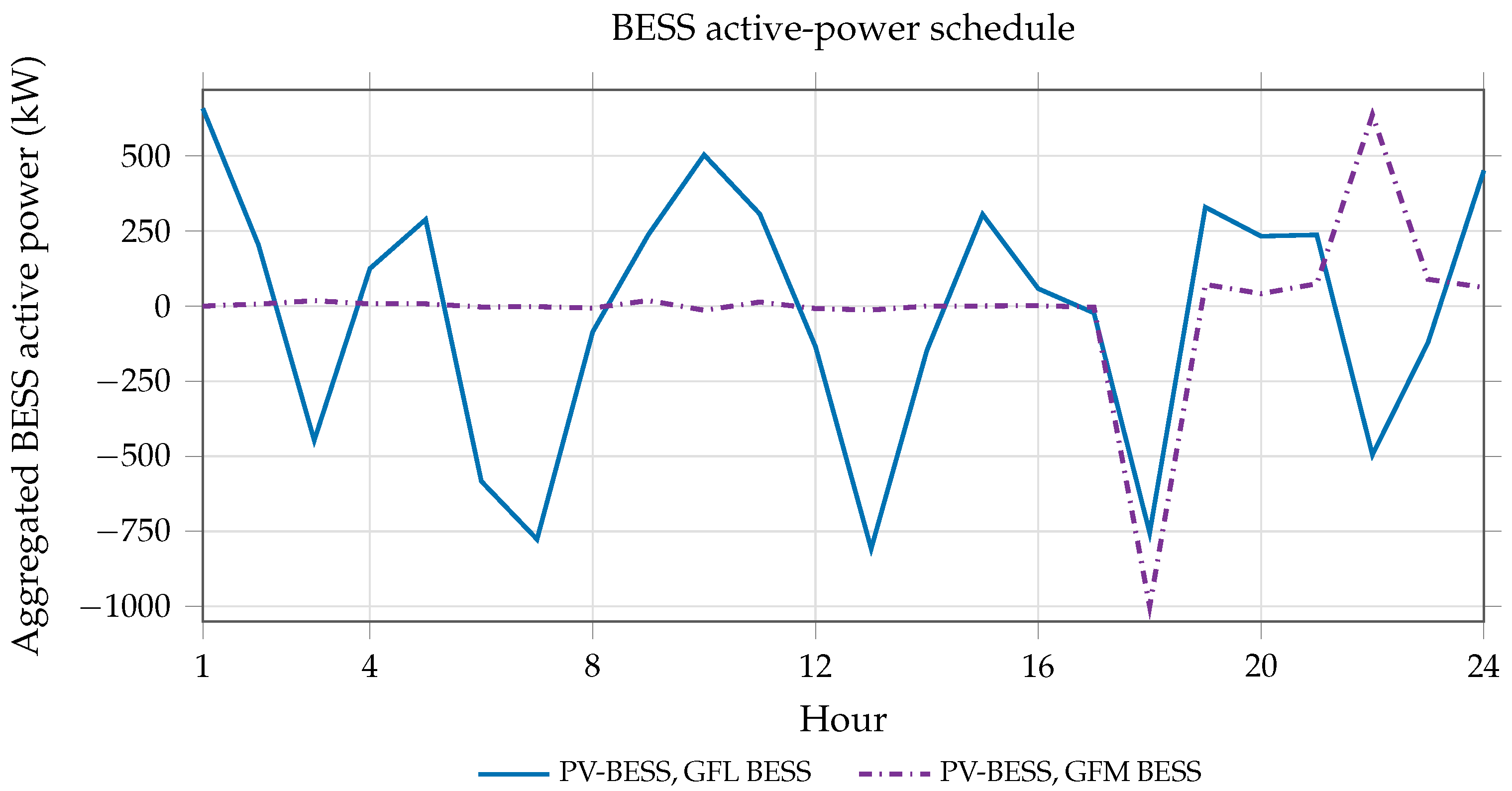
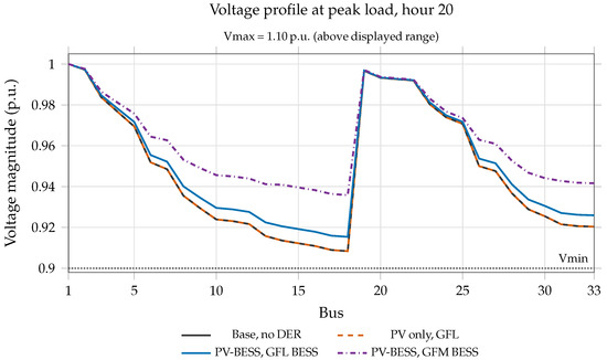
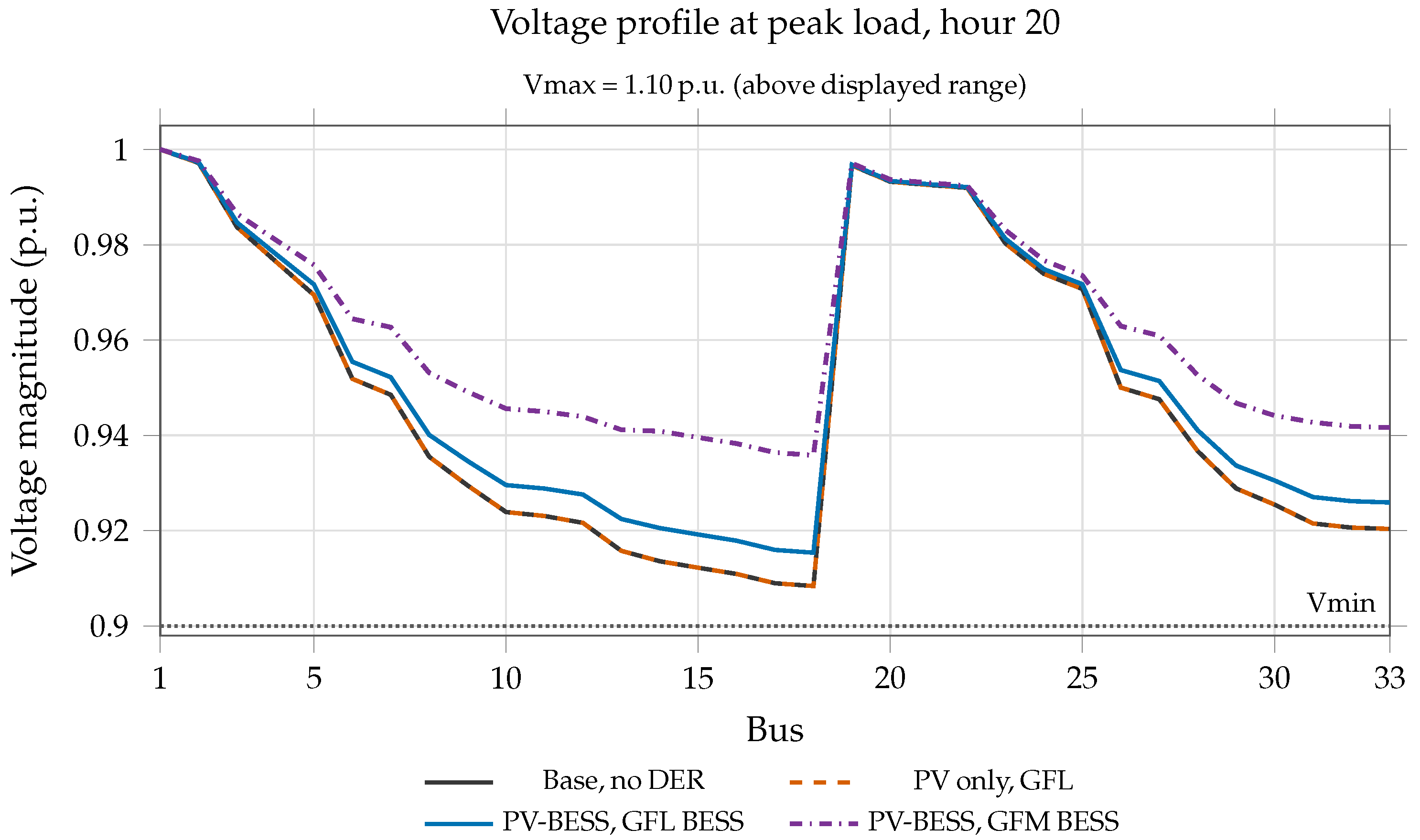
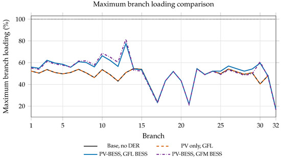
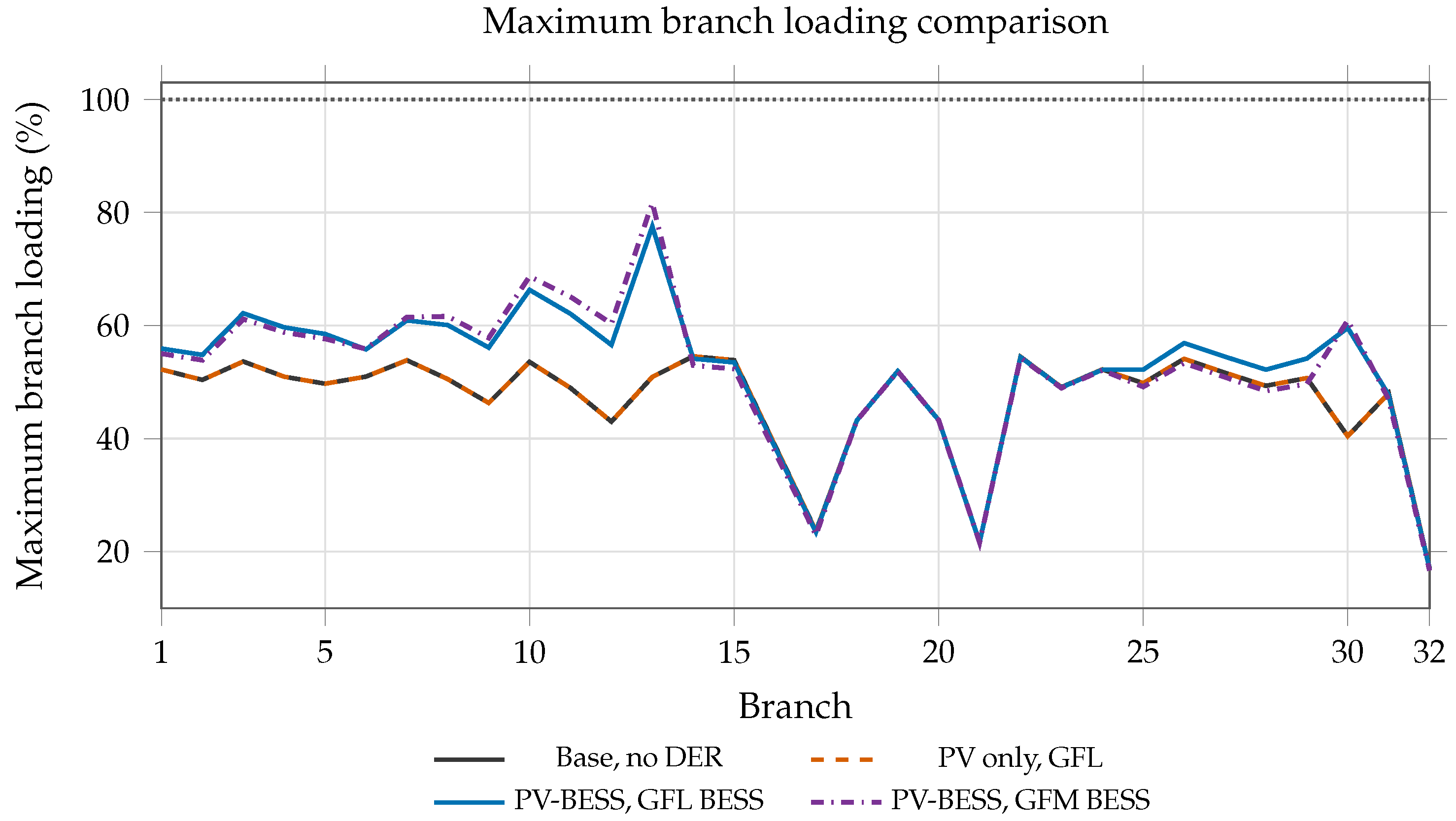
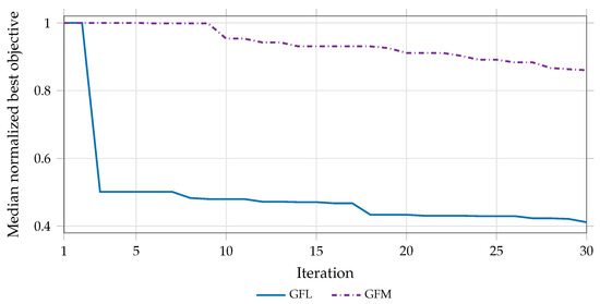
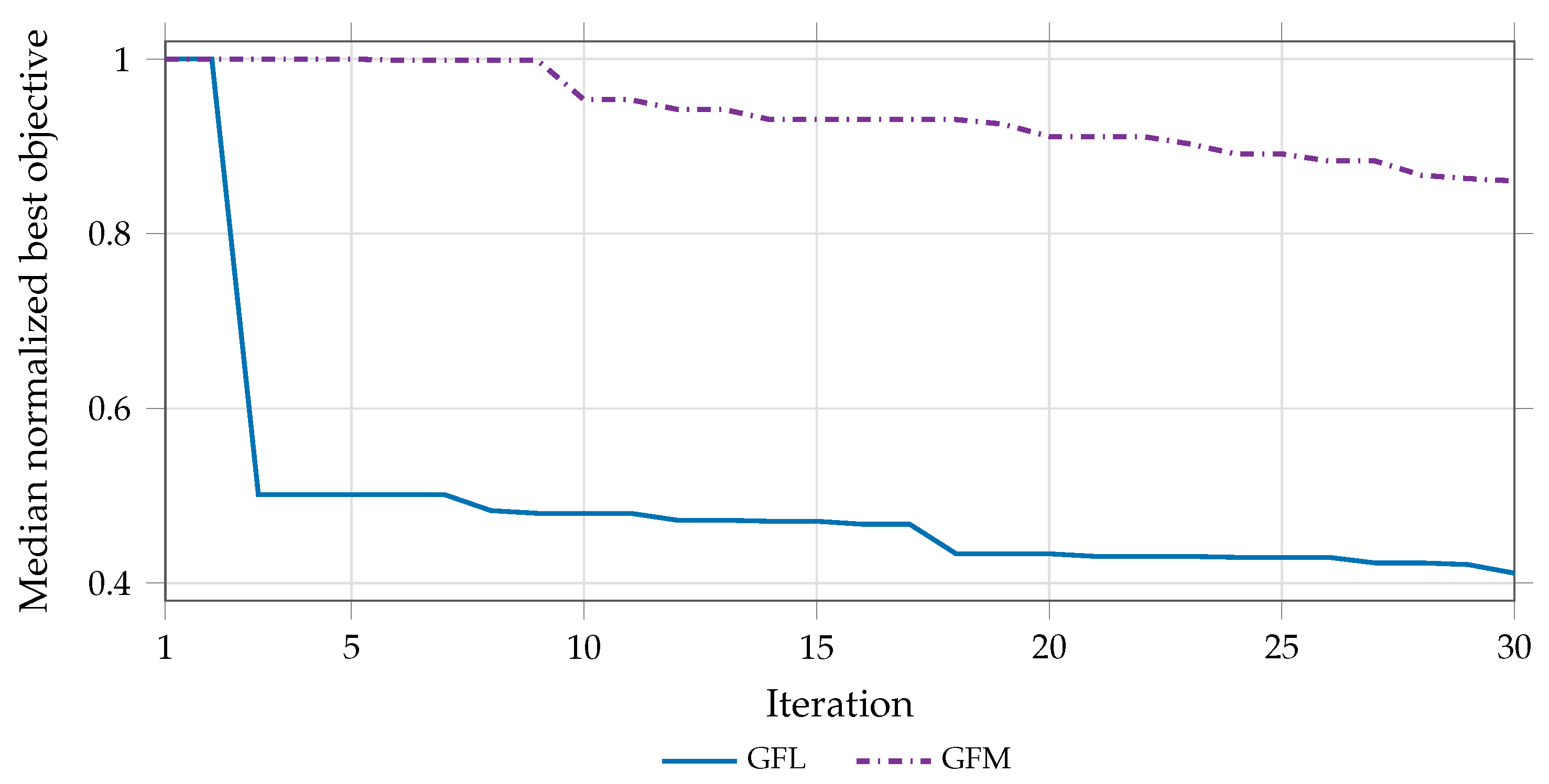
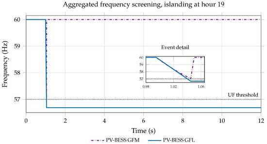
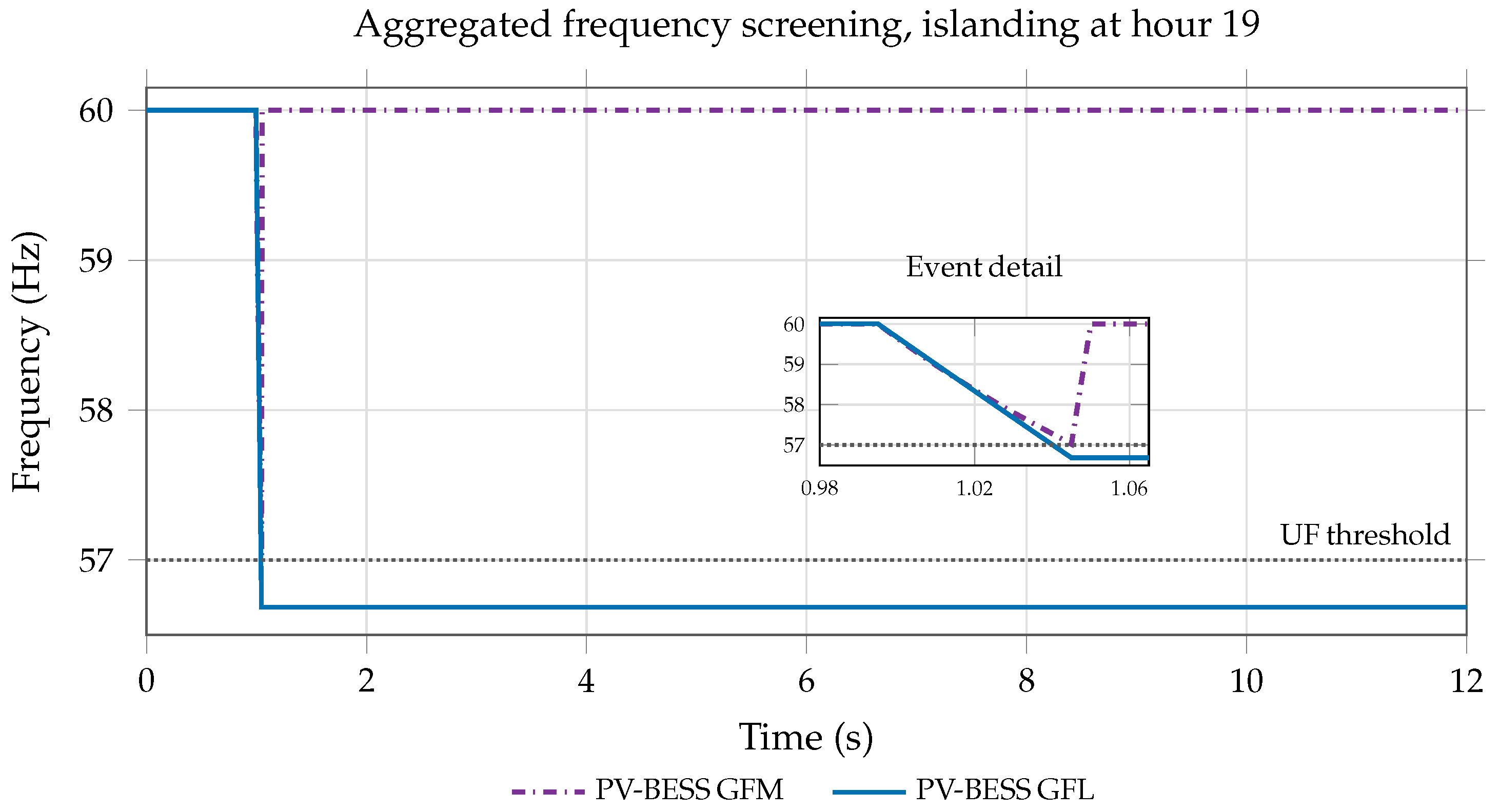

Disclaimer/Publisher’s Note: The statements, opinions and data contained in all publications are solely those of the individual author(s) and contributor(s) and not of MDPI and/or the editor(s). MDPI and/or the editor(s) disclaim responsibility for any injury to people or property resulting from any ideas, methods, instructions or products referred to in the content. |
© 2026 by the authors. Licensee MDPI, Basel, Switzerland. This article is an open access article distributed under the terms and conditions of the Creative Commons Attribution (CC BY) license.