Multi-Criteria Reduced-Order Modelling of Airport-Centric Microgrid for Frequency-Response Studies

Abstract

This article develops an analytic hierarchy process (AHP)-assisted model-reduction approach for a higher-order airport-centric microgrid (ACM). The full-order ACM model is approximated by a computationally simpler lower-order transfer function while retaining its essential steady-state and transient characteristics. The model approximation helps in analysis and controller design. For the same, a multi-objective fitness function is formulated from selected time moments and Markov parameters of the original and reduced models. AHP is used to determine the relative importance of the individual matching objectives through pairwise comparisons and normalized priority weights. The resulting weighted optimization problem is solved using the brown-bear optimization algorithm (BBOA) to estimate coefficients of the reduced model. During optimization, exact matching of steady-state gain is imposed to eliminate steady-state mismatch, while Hurwitz stability conditions ensure that the reduced model remains stable. Effectiveness of the proposed approach is evaluated using step and impulse responses, frequency-domain characteristics, time-domain specifications, and integral error indices. The results show that the AHP–BBOA-based reduced model closely reproduces the dominant dynamics of the higher-order ACM while offering a compact representation suitable for controller design, simulation, and real-time frequency-response studies.

1. Introduction

Microgrids provide a practical framework for integrating distributed generation, energy storage, local loads, and supervisory control within a defined electrical boundary [1]. Depending on their operating requirements, these may remain connected to the utility grid or continue supplying local loads in an islanded mode. Renewable sources such as photovoltaic arrays, wind turbines, fuel cells, and biomass-based generators can be coordinated with conventional generation to reduce dependence on the main grid. Energy-storage technologies, including batteries, flywheels, supercapacitors, and superconducting magnetic energy storage, further support power balancing during rapid variations in generation and demand [2,3]. These capabilities make microgrids relevant to facilities for which supply continuity, operational flexibility, and renewable-energy utilisation are important [4].

The structure of a microgrid depends strongly on the facility it serves. Community microgrids [5,6] are generally developed around residential loads and locally available energy resources, whereas industrial microgrids place greater emphasis on power quality and interruption costs. Marine systems [7,8] must operate under space limitations and rapidly changing loads, while campus microgrids [9,10] usually combine energy management with institutional sustainability objectives. Airport microgrids [11,12] form a separate category because these supply safety-critical, commercial, communication, and passenger-service loads within the same electrical network. A summary of these application-oriented configurations is given in Table 1.

Table 1. Application-oriented classification of microgrids.

Microgrid Type	Primary Purpose	Distinguishing Requirements	Representative Applications
Airport	Continuous supply to aviation-related and passenger-service loads	High supply reliability, redundancy, rapid recovery following a disturbance, and coordinated grid-connected and islanded operation	Airports, aviation hubs, and passenger terminals [11,12]
Campus	Coordinated energy management across institutional facilities	Integration of multiple buildings, distributed ownership, renewable-energy utilization, and support for sustainability studies	Universities, research institutions, hospitals, and corporate campuses [9,10]
Community	Local supply for residential consumers	Use of locally available renewable resources, shared storage, and reduced dependence on remote utility supply	Rural communities, residential neighbourhoods, and semi-urban settlements [5,6]
Industrial	Reliable and high-quality supply for production processes	Voltage and frequency regulation, limited interruption time, and coordination of process-dependent loads	Factories, manufacturing clusters, and data centres [13,14]
Marine	Electrical supply in maritime environments	Compact equipment, tolerance to harsh operating conditions, and management of rapidly changing propulsion and service loads	Ships, ports, offshore platforms, and coastal facilities [7,8]

Airports present an especially demanding microgrid application. Runway lighting, navigation aids, communication equipment, baggage-handling systems, security installations, data centres, and terminal services must operate with minimal interruption. At the same time, an airport may contain photovoltaic generation, standby generators, combined heat and power units, battery storage, electric-vehicle charging facilities, and highly variable commercial loads. An airport-centric microgrid (ACM) coordinates these resources within a common energy-management framework [11,12]. Its ability to isolate from the utility network and continue supplying priority loads can improve resilience of airport operations during external grid disturbances.

The dynamic behaviour of an ACM is governed by components with substantially different response rates. Power-electronic converters and storage devices can respond within short time intervals, whereas conventional generating units and controllable loads exhibit slower dynamics. Renewable generation and airport demand also vary independently. The combined effect of these elements produces a multi-time-scale system in which even a small generation-load imbalance can cause a measurable frequency deviation [15]. Accurate dynamic models are therefore required for frequency-response assessment, controller development, sensitivity analysis, and real-time simulation.

A detailed transfer-function representation can be formed by interconnecting the individual models of the generating units, storage systems, converters, and aggregate loads. Although such a representation captures the internal dynamics of the ACM, its overall order increases. A high-order model is useful for detailed offline studies but can make repeated simulation, controller tuning, optimisation, and hardware-in-the-loop implementation unnecessarily demanding. The presence of numerous poles and zeros may also obscure the small set of modes that primarily determine the observable system response. The lower-order models are easy to understand. The controller design also becomes easier for these models.

A lower-order model offers a more manageable representation, provided that reduction does not remove dynamics needed for intended study. Simple truncation or curve-fitting procedures may produce compact models, but reduction based only on one response characteristic does not necessarily preserve both low- and high-frequency behaviour. Similarly, a reduced model that matches a particular transient curve may have an incorrect steady-state gain or may fail to retain the stability of the original system. These limitations make stability preservation and systematic dynamic matching central requirements of model-order reduction [16,17].

Moment-based descriptions provide a useful basis for satisfying these requirements. The expansion of a transfer function about $s=0$ generates its time moments, which describe low-frequency and steady-state characteristics. Expansion about $s=\infty$ produces Markov parameters, which contain information about the short-time and high-frequency response. A reduced model obtained by considering both sets of coefficients can therefore represent a broader portion of original dynamics than a model constructed from only one expansion. Exact matching of the zeroth time moment preserves DC gain, whereas selected higher-order time moments and Markov parameters can be included as individual error objectives. The simultaneous treatment of several expansion errors introduces a weight-selection problem. Equal weighting is not always appropriate because the selected moments and parameters do not contribute identically to the quality of the approximation. Moreover, their numerical magnitudes can differ considerably.

In the present work, the analytic hierarchy process (AHP) is used to assign relative priorities to the individual matching objectives. Pairwise comparisons are arranged in a positive reciprocal matrix, from which a normalised priority vector is obtained. The consistency ratio is evaluated before the weights are accepted, thereby providing a check on the coherence of the assigned preferences. Once the AHP weights have been determined, the coefficients of the lower-order model are obtained by solving a constrained nonlinear optimisation problem. The objective function combines the normalised errors between selected time moments and Markov parameters of the higher- and lower-order models. Exact DC-gain matching is imposed as a steady-state constraint, while the Hurwitz conditions are used to restrict the search to stable reduced models. BBOA is employed to minimise the resulting weighted objective function [18]. Its population-based search uses pedal-marking and sniffing operators to update candidate coefficient vectors while retaining the better solutions generated during the search. Unlike a reduction procedure based exclusively on a step-response fit, the proposed formulation combines low-frequency matching, high-frequency matching, steady-state preservation, and stability in a single framework. AHP supplies the relative priorities of the matching objectives, whereas BBOA performs the numerical search for the reduced-model coefficients. The method is intended to produce a compact ACM representation without assuming that every coefficient of the higher-order transfer function contributes equally to the input–output response. The main contributions of this work are summarised as follows:

• A multi-objective model-reduction criterion is constructed from selected time moments and Markov parameters of the higher- and lower-order ACM models.
• AHP is used to obtain normalised weights for the individual matching errors, including an assessment of the consistency of the underlying pairwise judgements.
• BBOA is applied to determine the reduced-model coefficients subject to exact steady-state-gain matching and Hurwitz stability conditions.
• The reduced model is assessed using time- and frequency-domain responses, response specifications, and integral error indices relative to the original ACM model.

The remainder of this article is arranged as follows. The next section describes the architecture and transfer-function modelling of the airport-centric microgrid. The higher- and lower-order models and their time-moment and Markov-parameter expansions are then presented. The subsequent section formulates the weighted approximation problem and explains the AHP-based priority calculation. The BBOA search procedure and its application to the reduced-model coefficients are described next. Thereafter, the test system, numerical results, and comparative response analysis are reported. The final section summarises the principal findings and identifies possible extensions of the proposed reduction framework.

2. Architecture and Dynamic Model of Airport-Centric Microgrid

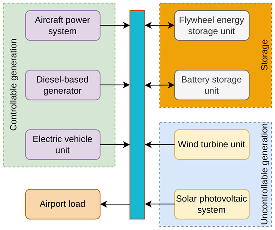
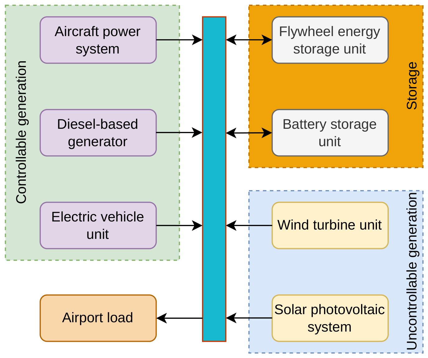
The airport-centric microgrid (ACM) considered in this study combines a wind turbine unit (WTU), solar-photovoltaic-system (SPS), aircraft power system (APS), diesel-based backup generator (DBBG), battery-storage unit (BSU), electric vehicle unit (EVU), and flywheel-energy-storage unit (FESU), as illustrated in Figure 1 [19,20]. The SPS, WTU, and DBBG primarily supply power, whereas the BSU and FESU can either absorb or inject energy. The APS and EVU may also provide bidirectional power support when their operating and state-of-charge limits permit. This combination enables the ACM to accommodate renewable-generation variations and changes in airport demand.

Figure 1. Architecture of the airport-centric microgrid.

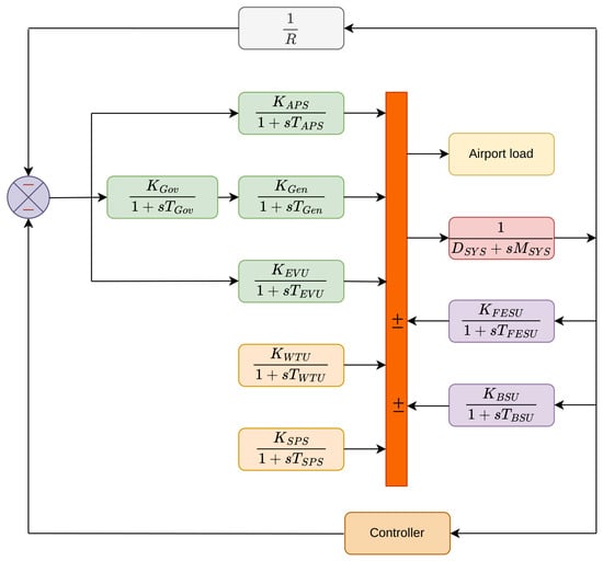
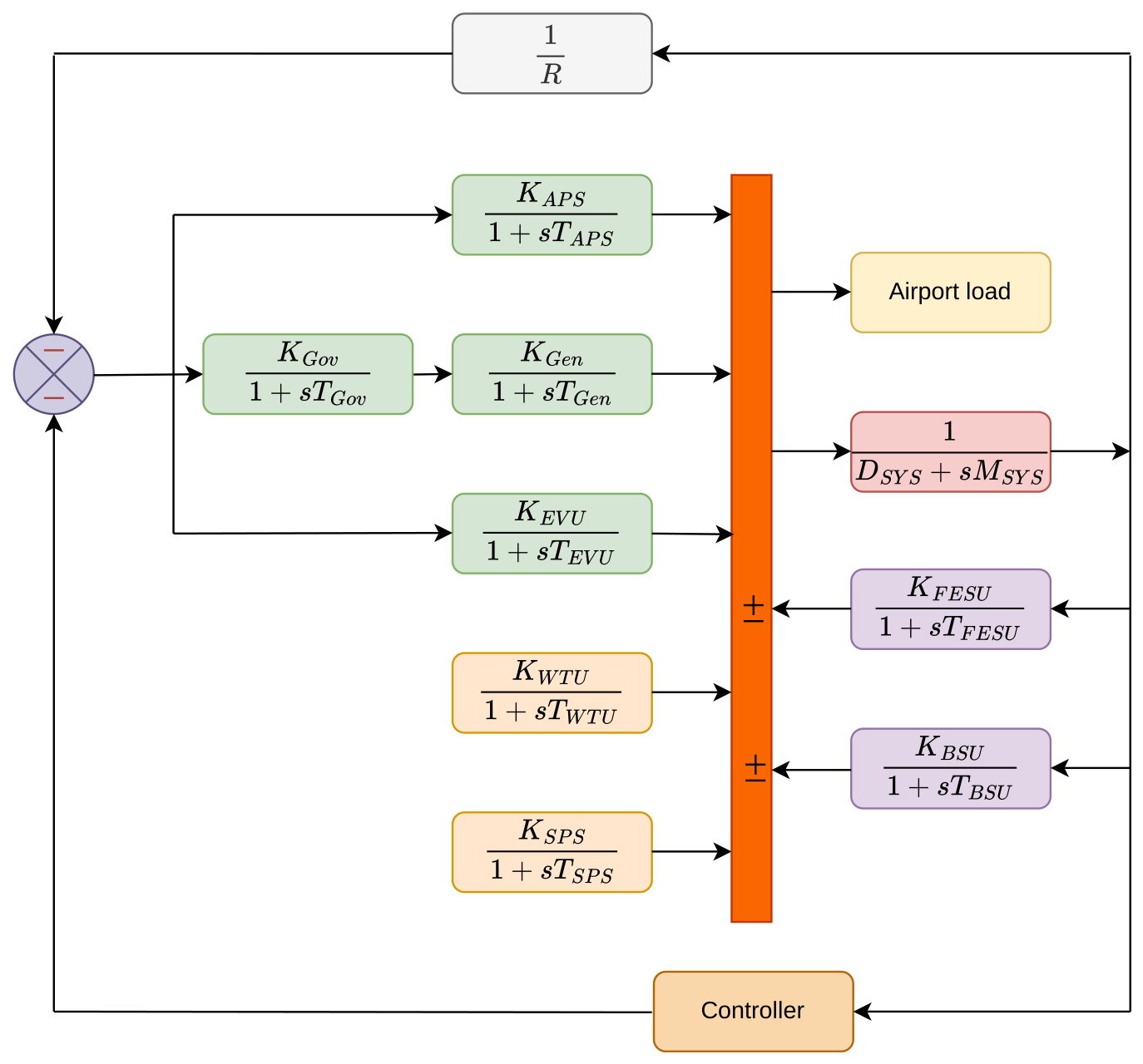
The dynamic interconnection of these components is shown in Figure 2 [19,20]. Each generation or storage unit is represented by its corresponding transfer-function model. Their incremental power outputs are combined with the load variation to determine the net power imbalance:

$$\begin{array}{cc}\hfill \Delta P_{\mathrm{net}}=& \Delta P_{\mathrm{SPS}}+\Delta P_{\mathrm{WTU}}+\Delta P_{\mathrm{DBBG}}+\Delta P_{\mathrm{APS}}+\Delta P_{\mathrm{EVU}}\hfill \\ \hfill & +\Delta P_{\mathrm{BSU}}+\Delta P_{\mathrm{FESU}}-\Delta P_L.\hfill \end{array}$$

(1)

In (1), the power contributions of the bidirectional units are treated as signed quantities: positive values indicate discharge into the ACM, while negative values represent charging. The resulting frequency deviation is governed by the equivalent inertia and damping of the microgrid:

$$\Delta f\left(s\right)={\displaystyle \frac{\Delta P_{\mathrm{net}}\left(s\right)}{D_{\mathrm{SYS}}+s{M}_{\mathrm{SYS}}}},$$

(2)

where $M_{\mathrm{SYS}}$ and $D_{\mathrm{SYS}}$ denote the equivalent inertia and damping coefficients, respectively.

Figure 2. Dynamic block diagram of the airport-centric microgrid.

After combining the individual component models and simplifying the block diagram, the overall high-order ACM transfer function [21] can be written as

$${\mathcal{G}}_p^{\mathrm{ACM}}\left(s\right)={\displaystyle \frac{\Delta f\left(s\right)}{U\left(s\right)}}={\displaystyle \frac{{\displaystyle {\displaystyle \sum _{i=0}^{p-1}}{\tilde{\alpha }}_i{s}^i}}{{\displaystyle {\displaystyle \sum _{j=0}^p}{\tilde{\beta }}_j{s}^j}}},$$

(3)

where $U\left(s\right)$ denotes the aggregate input to the ACM, ${\tilde{\alpha }}_i$ and ${\tilde{\beta }}_j$ are the resulting numerator and denominator coefficients, and p is the order of the complete system. The numerator and denominator coefficients are presented in Table 2 and Table 3, respectively. While obtaining these coefficients, regulation coefficient, R, is considered as 3. The high-order model in (3) forms the basis for developing the lower-order approximation.

Table 2. Numerator coefficients.

Coefficient	${\mathit{\alpha }}_0$	${\mathit{\alpha }}_1$	${\mathit{\alpha }}_2$	${\mathit{\alpha }}_3$	${\mathit{\alpha }}_4$	${\mathit{\alpha }}_5$
Value	3	$3.16$	$0.856$	$0.0972$	$0.0049$	$0.000088$

Table 3. Denominator coefficients.

Coefficient	${\mathit{\beta }}_0$	${\mathit{\beta }}_1$	${\mathit{\beta }}_2$	${\mathit{\beta }}_3$	${\mathit{\beta }}_4$	${\mathit{\beta }}_5$
Value	$3.012$	$4.0310933$	$1.45619733$	$0.2628096$	$0.028863973$	$0.0020384693$

3. Problem Description

3.1. Higher-Order System and Its Expansion Coefficients

Consider a stable, strictly proper, single-input single-output higher-order (HO) system of order p, represented by the rational transfer function

$${\mathcal{G}}_p\left(s\right)={\displaystyle \frac{{\displaystyle {\displaystyle \sum _{i=0}^{p-1}}{\tilde{\alpha }}_i{s}^i}}{{\displaystyle {\displaystyle \sum _{j=0}^p}{\tilde{\beta }}_j{s}^j}}}={\displaystyle \frac{{\tilde{\alpha }}_0+{\tilde{\alpha }}_{1}s+{\tilde{\alpha }}_2{s}^2+\cdots +{\tilde{\alpha }}_{p-1}{s}^{p-1}}{{\tilde{\beta }}_0+{\tilde{\beta }}_{1}s+{\tilde{\beta }}_2{s}^2+\cdots +{\tilde{\beta }}_p{s}^p}},$$

(4)

where ${\tilde{\alpha }}_i$, $i=0,1,\cdots ,p-1$, and ${\tilde{\beta }}_j$, $j=0,1,\cdots ,p$, denote numerator and denominator coefficients, respectively. It is assumed that ${\tilde{\beta }}_0\ne 0$ and ${\tilde{\beta }}_p\ne 0$.

The dynamic characteristics of ${\mathcal{G}}_p\left(s\right)$ can be expressed through two complementary series expansions. The expansion about the origin, $s=0$, characterises the low-frequency behaviour of the system and generates its time-moment sequence. Accordingly,

$${\mathcal{G}}_p\left(s\right)={\displaystyle \sum _{\mathsf{\ell }=0}^{\infty }}{\tilde{\mathfrak{m}}}_{\mathsf{\ell }}{s}^{\mathsf{\ell }}={\tilde{\mathfrak{m}}}_0+{\tilde{\mathfrak{m}}}_{1}s+{\tilde{\mathfrak{m}}}_2{s}^2+\cdots ,\hspace{1em}s\to 0,$$

(5)

where ${\tilde{\mathfrak{m}}}_{\mathsf{\ell }}$ denotes the ℓ-th time moment of the HO system.

Conversely, the expansion about $s=\infty$ describes the high-frequency behaviour and yields the Markov-parameter sequence:

$${\mathcal{G}}_p\left(s\right)={\displaystyle \sum _{\mathsf{\ell }=1}^{\infty }}{\tilde{\mathfrak{q}}}_{\mathsf{\ell }}{s}^{-\mathsf{\ell }}={\tilde{\mathfrak{q}}}_1{s}^{-1}+{\tilde{\mathfrak{q}}}_2{s}^{-2}+{\tilde{\mathfrak{q}}}_3{s}^{-3}+\cdots ,\hspace{1em}s\to \infty ,$$

(6)

where ${\tilde{\mathfrak{q}}}_{\mathsf{\ell }}$ represents the ℓ-th Markov parameter of ${\mathcal{G}}_p\left(s\right)$. Thus, the time moments and Markov parameters retain information associated with the low- and high-frequency dynamics, respectively.

3.2. Reduced-Order Model and Its Expansion Coefficients

Let the higher-order system in (4) be approximated by a strictly proper reduced-order model (ROM) of order r, where $r<p$. The ROM is expressed as

$${\mathcal{G}}_r^{\mathrm{red}}\left(s\right)={\displaystyle \frac{{\displaystyle {\displaystyle \sum _{i=0}^{r-1}}{\widehat{\alpha }}_i{s}^i}}{{\displaystyle {\displaystyle \sum _{j=0}^r}{\widehat{\beta }}_j{s}^j}}}={\displaystyle \frac{{\widehat{\alpha }}_0+{\widehat{\alpha }}_{1}s+{\widehat{\alpha }}_2{s}^2+\cdots +{\widehat{\alpha }}_{r-1}{s}^{r-1}}{{\widehat{\beta }}_0+{\widehat{\beta }}_{1}s+{\widehat{\beta }}_2{s}^2+\cdots +{\widehat{\beta }}_r{s}^r}},$$

(7)

where ${\widehat{\alpha }}_i$, $i=0,1,\cdots ,r-1$, and ${\widehat{\beta }}_j$, $j=0,1,\cdots ,r$, are unknown numerator and denominator coefficients of the ROM. These coefficients are selected so that ${\mathcal{G}}_r^{\mathrm{red}}\left(s\right)$ reproduces the important dynamic properties of the original system.

Expanding ${\mathcal{G}}_r^{\mathrm{red}}\left(s\right)$ about $s=0$ gives the time-moment representation

$${\mathcal{G}}_r^{\mathrm{red}}\left(s\right)={\displaystyle \sum _{\mathsf{\ell }=0}^{\infty }}{\widehat{\mathfrak{m}}}_{\mathsf{\ell }}{s}^{\mathsf{\ell }}={\widehat{\mathfrak{m}}}_0+{\widehat{\mathfrak{m}}}_{1}s+{\widehat{\mathfrak{m}}}_2{s}^2+\cdots ,\hspace{1em}s\to 0.$$

(8)

Similarly, its high-frequency expansion is

$${\mathcal{G}}_r^{\mathrm{red}}\left(s\right)={\displaystyle \sum _{\mathsf{\ell }=1}^{\infty }}{\widehat{\mathfrak{q}}}_{\mathsf{\ell }}{s}^{-\mathsf{\ell }}={\widehat{\mathfrak{q}}}_1{s}^{-1}+{\widehat{\mathfrak{q}}}_2{s}^{-2}+{\widehat{\mathfrak{q}}}_3{s}^{-3}+\cdots ,\hspace{1em}s\to \infty ,$$

(9)

where ${\widehat{\mathfrak{m}}}_{\mathsf{\ell }}$ and ${\widehat{\mathfrak{q}}}_{\mathsf{\ell }}$ are, respectively, the time moments and Markov parameters of the reduced-order model. A suitable approximation can therefore be constructed by enforcing the matching of selected expansion coefficients, namely,

$${\widehat{\mathfrak{m}}}_{\mathsf{\ell }}\approx {\tilde{\mathfrak{m}}}_{\mathsf{\ell }},\hspace{1em}{\widehat{\mathfrak{q}}}_{\nu }\approx {\tilde{\mathfrak{q}}}_{\nu },$$

(10)

for prescribed values of ℓ and $\nu$. Time-moment matching preserves the dominant low-frequency or steady-state characteristics, whereas Markov-parameter matching improves the reproduction of the short-time and high-frequency responses. For a second-order approximation, the formulation above is specialised by setting $r=2$.

3.3. Formulation of the Multi-Objective Optimisation Problem

The reduced-order model in (7) is constructed by retaining selected low- and high-frequency characteristics of the higher-order system described in (4). The time moments ${\tilde{\mathfrak{m}}}_{\mathsf{\ell }}$ and Markov parameters ${\tilde{\mathfrak{q}}}_{\mathsf{\ell }}$ of the original system are therefore compared with the corresponding quantities ${\widehat{\mathfrak{m}}}_{\mathsf{\ell }}$ and ${\widehat{\mathfrak{q}}}_{\mathsf{\ell }}$ of the reduced model.

The unknown coefficients of the ROM are collected into the decision vector

$${\mathit{\vartheta }}_r={\left[{\widehat{\alpha }}_0,{\widehat{\alpha }}_1,\dots ,{\widehat{\alpha }}_{r-1},{\widehat{\beta }}_0,{\widehat{\beta }}_1,\dots ,{\widehat{\beta }}_r\right]}^{\mathsf{T}}.$$

(11)

Since multiplying the numerator and denominator polynomials by the same nonzero constant does not alter the transfer function, one denominator coefficient may be fixed for normalisation. For example, ${\widehat{\beta }}_0=1$ can be imposed whenever ${\widehat{\beta }}_0\ne 0$.

To quantify the mismatch between the two models, normalised squared errors are defined for the selected time moments and Markov parameters:

$$\begin{array}{cc}\hfill {\mathcal{E}}_i^{\mathrm{TM}}\left({\mathit{\vartheta }}_r\right) & ={\left(1-{\displaystyle \frac{{\widehat{\mathfrak{m}}}_i}{{\tilde{\mathfrak{m}}}_i}}\right)}^2,\hspace{1em}i=1,2,\dots ,r-1,\hfill \end{array}$$

(12)

$$\begin{array}{cc}\hfill {\mathcal{E}}_j^{\mathrm{MP}}\left({\mathit{\vartheta }}_r\right) & ={\left(1-{\displaystyle \frac{{\widehat{\mathfrak{q}}}_j}{{\tilde{\mathfrak{q}}}_j}}\right)}^2,\hspace{1em}j=1,2,\dots ,r,\hfill \end{array}$$

(13)

The individual error measures are combined to obtain the following scalar objective function:

$$\mathcal{J}\left({\mathit{\vartheta }}_r\right)={\displaystyle \sum _{i=1}^{r-1}}{\varpi }_i^{\mathrm{TM}}{\mathcal{E}}_i^{\mathrm{TM}}\left({\mathit{\vartheta }}_r\right)+{\displaystyle \sum _{j=1}^r}{\varpi }_j^{\mathrm{MP}}{\mathcal{E}}_j^{\mathrm{MP}}\left({\mathit{\vartheta }}_r\right),$$

(14)

where ${\varpi }_i^{\mathrm{TM}}$ and ${\varpi }_j^{\mathrm{MP}}$ specify the relative importance assigned to the time-moment and Markov-parameter matching objectives, respectively. The weights are nonnegative and normalised according to

$${\varpi }_i^{\mathrm{TM}}\ge 0,\hspace{1em}{\varpi }_j^{\mathrm{MP}}\ge 0,\hspace{1em}{\displaystyle \sum _{i=1}^{r-1}}{\varpi }_i^{\mathrm{TM}}+{\displaystyle \sum _{j=1}^r}{\varpi }_j^{\mathrm{MP}}=1.$$

(15)

The optimisation problem can consequently be stated as

$$\begin{array}{cc}\hfill \underset{{\mathit{\vartheta }}_r}{\mathrm{minimize}} & \mathcal{J}\left({\mathit{\vartheta }}_r\right)\hfill \\ \hfill \mathrm{subject} \mathrm{to}& {\widehat{\mathfrak{m}}}_0={\tilde{\mathfrak{m}}}_0,\hfill \\ \hfill & {\Delta }_{\nu }\left(\widehat{\mathit{\beta }}\right)>0,\hspace{1em}\nu =1,2,\dots ,r,\hfill \end{array}$$

(16)

where

$$\widehat{\mathit{\beta }}={\left[{\widehat{\beta }}_0,{\widehat{\beta }}_1,\dots ,{\widehat{\beta }}_r\right]}^{\mathsf{T}},$$

and ${\Delta }_{\nu }(\widehat{\mathit{\beta }})$ denotes the $\nu$-th leading principal determinant of the Hurwitz matrix associated with the ROM denominator polynomial.

The first equality in (16) imposes exact matching of the zeroth time moment:

$${\mathcal{G}}_r^{\mathrm{red}}\left(0\right)={\mathcal{G}}_p\left(0\right) ⟺ {\widehat{\mathfrak{m}}}_0={\tilde{\mathfrak{m}}}_0.$$

(17)

For stable systems subjected to a step input, this condition ensures that the ROM reproduces the steady-state gain of the original system and thereby eliminates the steady-state mismatch between their responses. The Hurwitz-determinant inequalities impose asymptotic stability on the reduced model by requiring every pole of ${\mathcal{G}}_r^{\mathrm{red}}\left(s\right)$ to lie in the open left-half of the complex plane.

A total of $2r$ expansion coefficients are incorporated into the approximation procedure. The zeroth time moment is matched exactly through (17), whereas the remaining $r-1$ time moments and r Markov parameters constitute the $2r-1$ sub-objectives appearing in (14). This combined matching strategy allows the ROM to preserve both the low-frequency characteristics and the high-frequency transient behaviour of the original system.

The normalised priority coefficients ${\varpi }_i^{\mathrm{TM}}$ and ${\varpi }_j^{\mathrm{MP}}$ are determined using the analytic hierarchy process (AHP). Through pairwise comparisons, AHP converts the relative importance of the individual matching objectives into a consistent set of normalised weights. These weights are subsequently incorporated into (14) to guide the optimisation procedure toward the desired reduced-order approximation.

4. Analytic Hierarchy Process

The analytic hierarchy process (AHP) is employed to determine the relative contributions of the time-moment and Markov-parameter matching objectives appearing in (14). AHP converts qualitative judgements regarding the importance of different objectives into a normalised numerical weight vector. This is accomplished by arranging the decision elements hierarchically and comparing them in pairs.

In the present model-reduction problem, the overall goal is to obtain an accurate and stable reduced-order approximation. The decision criteria are the $r-1$ time-moment errors and the r Markov-parameter errors. Therefore, the total number of sub-objectives considered by AHP is

$$N_{\mathrm{o}}=(r-1)+r=2r-1.$$

(18)

The complete objective vector is organized as

$$\mathbf{\Phi }={\left[{\mathcal{E}}_1^{\mathrm{TM}},\dots ,{\mathcal{E}}_{r-1}^{\mathrm{TM}},{\mathcal{E}}_1^{\mathrm{MP}},\dots ,{\mathcal{E}}_r^{\mathrm{MP}}\right]}^{\mathsf{T}}\in {\mathbb{R}}^{N_{\mathrm{o}}},$$

(19)

where the individual error functions are defined in (12) and (13). The AHP procedure used to assign weights to these objectives is presented below.

Computational Procedure for AHP

• Step 1: Identification and prioritisation of the objectives

The first stage consists of identifying all the sub-objectives that influence the quality of the reduced-order approximation. Each pair of objectives is then assessed according to its relative importance. A judgement greater than unity indicates that the first objective is more important than the second, whereas a value smaller than unity indicates the opposite preference. A value of unity represents equal importance.

The fundamental numerical scale adopted for these comparisons is provided in Table 4. Intermediate even-numbered values may be used whenever the decision-maker’s preference lies between two adjacent qualitative judgements.

Table 4. Numerical scale for pairwise importance judgements.

Numerical Judgement	Interpretation
1	Equal importance
3	Moderate importance
5	Strong importance
7	Very strong importance
9	Extreme importance
2, 4, 6, 8	Intermediate levels of importance

If objective ${\Phi }_u$ is assigned a judgement $a_{uv}$ relative to ${\Phi }_v$, the reverse comparison is automatically assigned the reciprocal value $a_{vu}=1/a_{uv}$.

• Step 2: Construction of the reciprocal comparison matrix

The pairwise judgements are assembled into the positive reciprocal matrix

$$\mathsf{A}={\left[a_{uv}\right]}_{N_{\mathrm{o}}\times N_{\mathrm{o}}}=\left[\begin{array}{cccc}1 & a_{12} & \cdots & a_{1N_{\mathrm{o}}}\\ a_{21} & 1 & \cdots & a_{2N_{\mathrm{o}}}\\ ⋮ & ⋮ & \ddots & ⋮\\ a_{N_{\mathrm{o}}1} & a_{N_{\mathrm{o}}2} & \cdots & 1\end{array}\right],$$

(20)

in which $a_{uv}$ quantifies the importance of the u-th objective relative to the v-th objective. The entries of $\mathsf{A}$ satisfy

$$a_{uv}=\left\{\begin{array}{cc}1,\hfill & u=v,\hfill \\ a_{vu}^{-1},\hfill & u\ne v,\hfill \end{array}\right.\hspace{1em}{a}_{uv}>0.$$

(21)

Thus, only the entries located above or below the principal diagonal need to be independently specified.

• Step 3: Evaluation of row-wise geometric means

For every row of the comparison matrix, a geometric aggregation measure is computed as

$${\mathfrak{g}}_u={\left({\displaystyle \prod _{v=1}^{N_{\mathrm{o}}}}{a}_{uv}\right)}^{1/N_{\mathrm{o}}},\hspace{1em}u=1,2,\dots ,N_{\mathrm{o}},$$

(22)

where ${\mathfrak{g}}_u$ denotes the geometric mean associated with the u-th sub-objective. Collectively, these quantities form

$$\mathfrak{g}={\left[{\mathfrak{g}}_1,{\mathfrak{g}}_2,\dots ,{\mathfrak{g}}_{N_{\mathrm{o}}}\right]}^{\mathsf{T}}.$$

(23)

• Step 4: Derivation of normalised priority weights

The priority assigned to the u-th objective is obtained by normalising its geometric mean:

$${\varpi }_u={\displaystyle \frac{{\mathfrak{g}}_u}{{\displaystyle {\displaystyle \sum _{k=1}^{N_{\mathrm{o}}}}{\mathfrak{g}}_k}}},\hspace{1em}u=1,2,\dots ,N_{\mathrm{o}}.$$

(24)

The resulting priority vector is

$$\mathit{\varpi }={\left[{\varpi }_1,{\varpi }_2,\dots ,{\varpi }_{N_{\mathrm{o}}}\right]}^{\mathsf{T}},$$

(25)

and satisfies

$${\varpi }_u\ge 0,\hspace{1em}{\displaystyle \sum _{u=1}^{N_{\mathrm{o}}}}{\varpi }_u=1.$$

(26)

According to the ordering adopted in (19), the generic AHP priorities are mapped to the weights in (14) as

$$\begin{array}{cc}{\varpi }_i^{\mathrm{TM}}={\varpi }_i, \hfill & i=1,2,\dots ,r-1,\hfill \end{array}$$

(27)

$$\begin{array}{cccc}\hfill {\varpi }_j^{\mathrm{MP}}& ={\varpi }_{r-1+j}, \hfill & \hfill & j=1,2,\dots ,r.\hfill \end{array}$$

(28)

Consequently, the AHP-weighted objective function becomes

$$\mathcal{J}\left({\mathit{\vartheta }}_r\right)={\displaystyle \sum _{i=1}^{r-1}}{\varpi }_i{\mathcal{E}}_i^{\mathrm{TM}}\left({\mathit{\vartheta }}_r\right)+{\displaystyle \sum _{j=1}^r}{\varpi }_{r-1+j}{\mathcal{E}}_j^{\mathrm{MP}}\left({\mathit{\vartheta }}_r\right).$$

(29)

• Step 5: Verification of judgement consistency

Because pairwise assessments are based on relative preferences, their logical consistency should be examined before the weights are used. An estimate of the principal eigenvalue of the comparison matrix is obtained from

$${\rho }_{\max }={\displaystyle \frac{1}{N_{\mathrm{o}}}}{\displaystyle \sum _{u=1}^{N_{\mathrm{o}}}}{\displaystyle \frac{{\left(\mathsf{A}\varpi \right)}_u}{{\varpi }_u}}.$$

(30)

The consistency index is subsequently evaluated as

$${\mathcal{I}}_{\mathrm{C}}={\displaystyle \frac{{\rho }_{\max }-N_{\mathrm{o}}}{N_{\mathrm{o}}-1}}.$$

(31)

Using the random consistency index ${\mathcal{I}}_{\mathrm{R}}\left(N_{\mathrm{o}}\right)$, the consistency ratio is defined by

$${\mathcal{R}}_{\mathrm{C}}={\displaystyle \frac{{\mathcal{I}}_{\mathrm{C}}}{{\mathcal{I}}_{\mathrm{R}}\left(N_{\mathrm{o}}\right)}}.$$

(32)

The pairwise judgements are generally regarded as sufficiently consistent when

$${\mathcal{R}}_{\mathrm{C}}\le 0.10.$$

(33)

If this condition is not satisfied, the entries of $\mathsf{A}$ should be reviewed and revised before the priority weights are incorporated into the model-reduction optimisation. For $N_{\mathrm{o}}\le 2$, the comparison matrix is inherently consistent, and a consistency-ratio assessment is unnecessary.

5. Brown-Bear Optimisation Algorithm

The brown-bear optimisation algorithm (BBOA) is a population-based metaheuristic derived from the pedal scent-marking and sniffing patterns reported for brown bears [18]. In its mathematical interpretation, each bear group represents a candidate solution, while the pedal marks associated with that group represent the decision variables. The search process comprises a pedal-marking phase followed by a sniffing phase. Pedal marking provides three iteration-dependent search operators, whereas sniffing introduces pairwise movements among candidate solutions.

In the present study, a candidate solution contains the coefficients of the reduced-order model and is denoted by

$${\mathit{\vartheta }}_{r,i}^{\left(h\right)}={\left[{\vartheta }_{r,i,1}^{\left(h\right)},{\vartheta }_{r,i,2}^{\left(h\right)},\dots ,{\vartheta }_{r,i,K}^{\left(h\right)}\right]}^{\mathsf{T}},\hspace{1em}i=1,2,\dots ,M,$$

(34)

where M is the population size, K is the number of independent decision variables, and h denotes the current iteration. The vector ${\mathit{\vartheta }}_{r,i}^{\left(h\right)}$ follows the coefficient arrangement introduced in (11), after accounting for the selected denominator normalisation.

The fitness of a candidate is evaluated using the AHP-weighted objective function developed in (29):

$$\mathcal{F}\left({\mathit{\vartheta }}_{r,i}^{\left(h\right)}\right)=\mathcal{J}\left({\mathit{\vartheta }}_{r,i}^{\left(h\right)}\right).$$

(35)

The steady-state, stability, normalisation, and parameter-bound constraints specified in (16) are enforced during fitness evaluation. An infeasible candidate is either repaired or assigned a sufficiently large penalised fitness value.

5.1. Population Initialization

Let ${\underline{\vartheta }}_j$ and ${\overline{\vartheta }}_j$ denote the lower and upper limits of the j-th decision variable. The initial population is sampled as

$${\vartheta }_{r,i,j}^{\left(0\right)}={\underline{\vartheta }}_j+{\mathfrak{u}}_{i,j}^{\left(0\right)}\left({\overline{\vartheta }}_j-{\underline{\vartheta }}_j\right),$$

(36)

where

$${\mathfrak{u}}_{i,j}^{\left(0\right)}\sim \mathcal{U}(0,1),\hspace{1em}i=1,2,\dots ,M,\hspace{1em}j=1,2,\dots ,K.$$

Thus, the population at iteration h is represented by

$${\mathsf{V}}^{\left(h\right)}=\left[\begin{array}{c}{\left({\mathit{\vartheta }}_{r,1}^{\left(h\right)}\right)}^{\mathsf{T}}\\ {\left({\mathit{\vartheta }}_{r,2}^{\left(h\right)}\right)}^{\mathsf{T}}\\ ⋮\\ {\left({\mathit{\vartheta }}_{r,M}^{\left(h\right)}\right)}^{\mathsf{T}}\end{array}\right]\in {\mathbb{R}}^{M\times K}.$$

(37)

At every iteration, the candidates with the smallest and largest fitness values are identified as

$$\begin{array}{cc}\hfill {\mathit{\vartheta }}_{r,\star }^{\left(h\right)} & =\underset{{\mathit{\vartheta }}_{r,i}^{\left(h\right)}\in {\mathsf{V}}^{\left(h\right)}}{\arg \min } \mathcal{F}\left({\mathit{\vartheta }}_{r,i}^{\left(h\right)}\right),\hfill \end{array}$$

(38)

$$\begin{array}{cc}\hfill {\mathit{\vartheta }}_{r,†}^{\left(h\right)} & =\underset{{\mathit{\vartheta }}_{r,i}^{\left(h\right)}\in {\mathsf{V}}^{\left(h\right)}}{\arg \max } \mathcal{F}\left({\mathit{\vartheta }}_{r,i}^{\left(h\right)}\right).\hfill \end{array}$$

(39)

For a maximum iteration count $N_{\mathrm{iter}}$, the normalised iteration index is

$${\tau }_h={\displaystyle \frac{h}{N_{\mathrm{iter}}}},\hspace{1em}0<{\tau }_h\le 1.$$

(40)

This factor separates the pedal-marking phase into three consecutive search regimes.

5.2. Pedal Scent-Marking Phase

The pedal scent-marking phase applies a different update rule during each third of the optimisation run.

5.2.1. Gait-Based Update

During the first third of the iterations, each candidate is modified through a stochastic scaling operation:

$${\zeta }_{i,j}^{\left(h\right)}={\vartheta }_{r,i,j}^{\left(h\right)}-{\tau }_h {\mathfrak{u}}_{i,j}^{\left(h\right)}{\vartheta }_{r,i,j}^{\left(h\right)},\hspace{1em}0<{\tau }_h\le {\displaystyle \frac{1}{3}},$$

(41)

where ${\mathfrak{u}}_{i,j}^{\left(h\right)}\sim \mathcal{U}(0,1)$. The variable ${\zeta }_{i,j}^{\left(h\right)}$ denotes the j-th component of the trial vector produced by the pedal-marking operation.

5.2.2. Careful-Stepping Update

During the middle third, the update uses information from the best and worst members of the current population:

$${\zeta }_{i,j}^{\left(h\right)}={\vartheta }_{r,i,j}^{\left(h\right)}+{\mathcal{F}}_h\left({\vartheta }_{r,\star ,j}^{\left(h\right)}-{\mathcal{L}}_h{\vartheta }_{r,†,j}^{\left(h\right)}\right),\hspace{1em}{\displaystyle \frac{1}{3}}<{\tau }_h\le {\displaystyle \frac{2}{3}}.$$

(42)

The step factor ${\mathcal{F}}_h$ is calculated from

$${\mathcal{F}}_h={\mathfrak{u}}_{1,h}{\tau }_h,\hspace{1em}{\mathfrak{u}}_{1,h}\sim \mathcal{U}(0,1),$$

(43)

whereas the discrete step length is

$${\mathcal{L}}_h=\mathrm{round}\left(1+{\mathfrak{u}}_{2,h}\right)\in \{1,2\},\hspace{1em}{\mathfrak{u}}_{2,h}\sim \mathcal{U}(0,1).$$

(44)

The best candidate supplies an attractive direction, while the worst candidate modifies the magnitude and orientation of the trial displacement.

5.2.3. Twisting-Feet Update

The final third of the pedal-marking phase employs a rotational scaling coefficient

$${\Omega }_{i,h}=2\pi {\tau }_h{\mathfrak{u}}_{i,h},\hspace{1em}{\mathfrak{u}}_{i,h}\sim \mathcal{U}(0,1).$$

(45)

The trial point is then generated from

$$\begin{array}{cc}\hfill {\zeta }_{i,j}^{\left(h\right)}=& {\vartheta }_{r,i,j}^{\left(h\right)}+{\Omega }_{i,h}\left({\vartheta }_{r,\star ,j}^{\left(h\right)}-\left|{\vartheta }_{r,i,j}^{\left(h\right)}\right|\right)\hfill \\ \hfill & -{\Omega }_{i,h}\left({\vartheta }_{r,†,j}^{\left(h\right)}-\left|{\vartheta }_{r,i,j}^{\left(h\right)}\right|\right),\hspace{1em}{\displaystyle \frac{2}{3}}<{\tau }_h\le 1.\hfill \end{array}$$

(46)

Equations (41), (42) and (46) can be summarised as

$${\zeta }_{i,j}^{\left(h\right)}=\left\{\begin{array}{cc}{\vartheta }_{r,i,j}^{\left(h\right)}-{\tau }_h{\mathfrak{u}}_{i,j}^{\left(h\right)}{\vartheta }_{r,i,j}^{\left(h\right)}, \hfill & 0<{\tau }_h\le {\displaystyle \frac{1}{3}},\hfill \\ {\vartheta }_{r,i,j}^{\left(h\right)}+{\mathcal{F}}_h\left({\vartheta }_{r,\star ,j}^{\left(h\right)}-{\mathcal{L}}_h{\vartheta }_{r,†,j}^{\left(h\right)}\right), \hfill & {\displaystyle \frac{1}{3}}<{\tau }_h\le {\displaystyle \frac{2}{3}},\hfill \\ {\vartheta }_{r,i,j}^{\left(h\right)}+{\Omega }_{i,h}\left({\vartheta }_{r,\star ,j}^{\left(h\right)}-\left|{\vartheta }_{r,i,j}^{\left(h\right)}\right|\right)-{\Omega }_{i,h}\left({\vartheta }_{r,†,j}^{\left(h\right)}-\left|{\vartheta }_{r,i,j}^{\left(h\right)}\right|\right), \hfill & {\displaystyle \frac{2}{3}}<{\tau }_h\le 1.\hfill \end{array}\right.$$

(47)

A component falling outside its permitted interval is returned to the search domain using

$${\mathcal{B}}_j\left(x\right)=\min \left\{{\overline{\vartheta }}_j,\max \left\{{\underline{\vartheta }}_j,x\right\}\right\}.$$

(48)

Accordingly, the repaired pedal-marking vector is

$${\tilde{\mathit{\zeta }}}_i^{\left(h\right)}={\left[{\mathcal{B}}_1\left({\zeta }_{i,1}^{\left(h\right)}\right),\dots ,{\mathcal{B}}_K\left({\zeta }_{i,K}^{\left(h\right)}\right)\right]}^{\mathsf{T}}.$$

(49)

A greedy comparison retains the better of the original and trial vectors:

$${\overline{\mathit{\vartheta }}}_{r,i}^{\left(h\right)}=\left\{\begin{array}{cc}{\tilde{\mathit{\zeta }}}_i^{\left(h\right)}, \hfill & \mathcal{F}\left({\tilde{\mathit{\zeta }}}_i^{\left(h\right)}\right)\le \mathcal{F}\left({\mathit{\vartheta }}_{r,i}^{\left(h\right)}\right),\hfill \\ {\mathit{\vartheta }}_{r,i}^{\left(h\right)}, \hfill & \mathrm{otherwise}.\hfill \end{array}\right.$$

(50)

5.3. Sniffing Phase

Following pedal marking, each population member ${\overline{\mathit{\vartheta }}}_{r,a}^{\left(h\right)}$ is paired with a randomly selected member ${\overline{\mathit{\vartheta }}}_{r,b}^{\left(h\right)}$, where $a\ne b$. The sniffing trial vector is generated componentwise as

$${\upsilon }_{a,j}^{\left(h\right)}=\left\{\begin{array}{cc}{\overline{\vartheta }}_{r,a,j}^{\left(h\right)}+{\mathfrak{s}}_{a,j}^{\left(h\right)}\left({\overline{\vartheta }}_{r,a,j}^{\left(h\right)}-{\overline{\vartheta }}_{r,b,j}^{\left(h\right)}\right), \hfill & \mathcal{F}\left({\overline{\mathit{\vartheta }}}_{r,a}^{\left(h\right)}\right)<\mathcal{F}\left({\overline{\mathit{\vartheta }}}_{r,b}^{\left(h\right)}\right),\hfill \\ {\overline{\vartheta }}_{r,a,j}^{\left(h\right)}+{\mathfrak{s}}_{a,j}^{\left(h\right)}\left({\overline{\vartheta }}_{r,b,j}^{\left(h\right)}-{\overline{\vartheta }}_{r,a,j}^{\left(h\right)}\right), \hfill & \mathcal{F}\left({\overline{\mathit{\vartheta }}}_{r,b}^{\left(h\right)}\right)<\mathcal{F}\left({\overline{\mathit{\vartheta }}}_{r,a}^{\left(h\right)}\right),\hfill \\ {\overline{\vartheta }}_{r,a,j}^{\left(h\right)}, \hfill & \mathrm{otherwise},\hfill \end{array}\right.$$

(51)

where ${\mathfrak{s}}_{a,j}^{\left(h\right)}\sim \mathcal{U}(0,1)$. The first condition moves the better candidate away from the inferior one, whereas the second moves the inferior candidate toward the better member.

After boundary correction, the sniffing trial vector is written as

$${\tilde{\mathit{\upsilon }}}_a^{\left(h\right)}={\left[{\mathcal{B}}_1\left({\upsilon }_{a,1}^{\left(h\right)}\right),\dots ,{\mathcal{B}}_K\left({\upsilon }_{a,K}^{\left(h\right)}\right)\right]}^{\mathsf{T}}.$$

(52)

The population entering the next iteration is selected according to

$${\mathit{\vartheta }}_{r,a}^{(h+1)}=\left\{\begin{array}{cc}{\tilde{\mathit{\upsilon }}}_a^{\left(h\right)}, \hfill & \mathcal{F}\left({\tilde{\mathit{\upsilon }}}_a^{\left(h\right)}\right)\le \mathcal{F}\left({\overline{\mathit{\vartheta }}}_{r,a}^{\left(h\right)}\right),\hfill \\ {\overline{\mathit{\vartheta }}}_{r,a}^{\left(h\right)}, \hfill & \mathrm{otherwise}.\hfill \end{array}\right.$$

(53)

The pedal-marking operators conduct structured refinement using the current population and its extreme members. The sniffing operator supplements this process with pairwise displacements, thereby retaining population diversity. Greedy selection after both phases prevents deterioration of the accepted fitness values. The detailed computation procedure using BBOA is given in Table 5.

Table 5. Computational procedure of BBOA.

Input: Population size M, dimension K, maximum iterations $N_{\mathrm{iter}}$, bounds $\underline{\mathit{\vartheta }}$ and $\overline{\mathit{\vartheta }}$, and fitness function $F\left({\mathit{\vartheta }}_r\right)$.

Output: Best ROM coefficient vector ${\vartheta }_{r,\star }$ and its fitness ${\mathcal{F}}_{\star }$.

1: Generate M candidate solutions using (36).

2: Repair or reject infeasible candidates and evaluate their fitness values.

3: Set $h\leftarrow 1$, and record the best feasible candidate.

4:  while  $h\le N_{\mathrm{iter}}$  do

4.1: Determine ${\mathit{\vartheta }}_{r,\star }^{\left(h\right)}$ and ${\mathit{\vartheta }}_{r,†}^{\left(h\right)}$ from (38) and (39).

4.2: Calculate ${\tau }_h=h/N_{\mathrm{iter}}$.

4.3: For every candidate, generate a pedal-marking trial vector using (47).

If $0<{\tau }_h\le 1/3$, apply the gait-based update.

If $1/3<{\tau }_h\le 2/3$, apply the careful-stepping update.

If $2/3<{\tau }_h\le 1$, apply the twisting-feet update.

4.4: Apply the boundary and feasibility rules, evaluate the pedal-marking trials, and retain candidates according to (50).

4.5: For each candidate a, randomly select $b\ne a$ and generate a sniffing trial using (51).

4.6: Repair the sniffing trials, evaluate their fitness values, and update the population using (53).

4.7: Update the global-best solution if a lower fitness value has been found.

4.8: Set $h\leftarrow h+1$.

5:  end while

6: Return ${\mathit{\vartheta }}_{r,\star }$ and ${\mathcal{F}}_{\star }$.

6. Test System and Results

6.1. ACM Test Case and Stability Check

The ACM architecture and its general high-order representation are already introduced in Section 2. Thus, only the numerical model required for the reduction study is stated here. Using the coefficients listed in Table 2 and Table 3, the fifth-order test system is

$${\mathcal{G}}_5^{\mathrm{ACM}}\left(s\right)={\displaystyle \frac{3+3.16s+0.856s^2+0.0972s^3+0.0049s^4+0.000088s^5}{3.012+4.0310933s+1.45619733s^2+0.2628096s^3+0.028863973s^4+0.0020384693s^5}}.$$

(54)

The numerator and denominator have the same degree, so (54) is proper rather than strictly proper. Its poles are

$$s=-1.11779,\hspace{1em}s=-4.54334\pm \mathrm{j}1.97409,\hspace{1em}s=-1.97759\pm \mathrm{j}7.06809.$$

(55)

Since every pole has a negative real part, the test system is asymptotically stable.

6.2. Isolation of Strictly Proper Dynamics

Direct reduction of a biproper transfer function can distort its high-frequency gain. To avoid this, polynomial division is used to separate the constant feedthrough term from the dynamic part:

$${\mathcal{G}}_5^{\mathrm{ACM}}\left(s\right)=d_{\mathrm{ACM}}+{\mathcal{G}}_{5,\mathrm{sp}}^{\mathrm{ACM}}\left(s\right),$$

(56)

where

$$d_{\mathrm{ACM}}={\displaystyle \frac{{\tilde{\alpha }}_5}{{\tilde{\beta }}_5}}={\displaystyle \frac{0.000088}{0.0020384693}}=0.04316964695.$$

(57)

The residual dynamics are consequently described by

$${\mathcal{G}}_{5,\mathrm{sp}}^{\mathrm{ACM}}\left(s\right)={\displaystyle \frac{{\mathcal{N}}_{\mathrm{sp}}\left(s\right)}{{\mathcal{D}}_5\left(s\right)}},$$

(58)

with

$$\begin{array}{cc}\hfill {\mathcal{N}}_{\mathrm{sp}}\left(s\right)=& 2.869973023+2.985979125s+0.7931364754s^2\hfill \\ \hfill & +0.08585460235s^3+0.003653952476s^4,\hfill \end{array}$$

(59)

and

$$\begin{array}{cc}\hfill {\mathcal{D}}_5\left(s\right)=& 3.012+4.0310933s+1.45619733s^2\hfill \\ \hfill & +0.2628096s^3+0.028863973s^4+0.0020384693s^5.\hfill \end{array}$$

(60)

This residual has zero gain as $s\to \infty$, whereas $d_{\mathrm{ACM}}$ preserves the original limiting gain exactly.

6.3. Expansion Data for Model Reduction

Around the origin, the residual transfer function has the series

$$\begin{array}{cc}\hfill {\mathcal{G}}_{5,\mathrm{sp}}^{\mathrm{ACM}}\left(s\right)=& 0.9528462893-0.2838755536s+0.1825807088s^2\hfill \\ \hfill & -0.1617475427s^3+0.1450538309s^4+\mathcal{O}\left(s^5\right).\hfill \end{array}$$

(61)

The two low-frequency coefficients retained for this study are

$${\tilde{\mathfrak{m}}}_0^{\mathrm{sp}}=0.9528462893,\hspace{1em}{\tilde{\mathfrak{m}}}_1^{\mathrm{sp}}=-0.2838755536.$$

(62)

The corresponding expansion at infinity is

$$\begin{array}{cc}\hfill {\mathcal{G}}_{5,\mathrm{sp}}^{\mathrm{ACM}}\left(s\right)=& 1.792498163s^{-1}+16.73607926s^{-2}-78.99014702s^{-3}\hfill \\ \hfill & -854.89869197s^{-4}+8196.519547s^{-5}+\mathcal{O}\left(s^{-6}\right).\hfill \end{array}$$

(63)

Its first two Markov parameters are

$${\tilde{\mathfrak{q}}}_1^{\mathrm{sp}}=1.792498163,\hspace{1em}{\tilde{\mathfrak{q}}}_2^{\mathrm{sp}}=16.73607926.$$

(64)

Separating the feedthrough term affects only the constant term in the low-frequency expansion; the remaining time moments and the strictly proper Markov sequence are unchanged.

6.4. Second-Order Residual Model

The fifth-order residual is represented by the second-order structure

$${\widehat{\mathcal{G}}}_{2,\mathrm{sp}}^{\mathrm{ACM}}\left(s\right)={\displaystyle \frac{{\widehat{\alpha }}_0+{\widehat{\alpha }}_{1}s}{{\widehat{\beta }}_0+{\widehat{\beta }}_{1}s+{\widehat{\beta }}_2{s}^2}}.$$

(65)

The unknown coefficient vector is

$${\mathit{\vartheta }}_2={\left[{\widehat{\alpha }}_0,{\widehat{\alpha }}_1,{\widehat{\beta }}_0,{\widehat{\beta }}_1,{\widehat{\beta }}_2\right]}^{\mathsf{T}}.$$

(66)

The expansion coefficients needed in the objective function follow directly from (65):

$$\begin{array}{cc}\hfill {\widehat{\mathfrak{m}}}_0^{\mathrm{sp}} & ={\displaystyle \frac{{\widehat{\alpha }}_0}{{\widehat{\beta }}_0}},\hfill \end{array}$$

(67)

$$\begin{array}{cc}\hfill {\widehat{\mathfrak{m}}}_1^{\mathrm{sp}} & ={\displaystyle \frac{{\widehat{\alpha }}_1{\widehat{\beta }}_0-{\widehat{\alpha }}_0{\widehat{\beta }}_1}{{\widehat{\beta }}_0^2}}.\hfill \end{array}$$

(68)

$$\begin{array}{cc}\hfill {\widehat{\mathfrak{q}}}_1^{\mathrm{sp}} & ={\displaystyle \frac{{\widehat{\alpha }}_1}{{\widehat{\beta }}_2}},\hfill \end{array}$$

(69)

$$\begin{array}{cc}\hfill {\widehat{\mathfrak{q}}}_2^{\mathrm{sp}} & ={\displaystyle \frac{{\widehat{\alpha }}_0{\widehat{\beta }}_2-{\widehat{\alpha }}_1{\widehat{\beta }}_1}{{\widehat{\beta }}_2^2}}.\hfill \end{array}$$

(70)

6.5. AHP-Weighted Reduction Problem

Because the zeroth time moment is imposed as an equality constraint, the optimisation uses the normalised mismatch in the first time moment and the first two Markov parameters:

$$\begin{array}{cc}\hfill {\mathcal{E}}_1^{\mathrm{TM}} & ={\left(1-{\displaystyle \frac{{\widehat{\mathfrak{m}}}_1}{{\tilde{\mathfrak{m}}}_1}}\right)}^2,\hfill \end{array}$$

(71)

$$\begin{array}{cc}\hfill {\mathcal{E}}_1^{\mathrm{MP}} & ={\left(1-{\displaystyle \frac{{\widehat{\mathfrak{q}}}_1}{{\tilde{\mathfrak{q}}}_1}}\right)}^2,\hfill \end{array}$$

(72)

$$\begin{array}{cc}\hfill {\mathcal{E}}_2^{\mathrm{MP}} & ={\left(1-{\displaystyle \frac{{\widehat{\mathfrak{q}}}_2}{{\tilde{\mathfrak{q}}}_2}}\right)}^2.\hfill \end{array}$$

(73)

Low-frequency fidelity is given the greatest importance, followed by the leading and second high-frequency coefficients. Applying the AHP scale in this order gives the reciprocal matrix

$${\mathsf{A}}_{\mathrm{ACM}}=\left[\begin{array}{ccc}1& 3& 5\\ 1/3& 1& 3\\ 1/5& 1/3& 1\end{array}\right].$$

(74)

The rows and columns correspond, respectively, to ${\mathcal{E}}_1^{\mathrm{TM}}$, ${\mathcal{E}}_1^{\mathrm{MP}}$, and ${\mathcal{E}}_2^{\mathrm{MP}}$. Row-geometric-mean normalization yields

$${\mathit{\varpi }}_{\mathrm{AHP}}=\left[\begin{array}{c}{\varpi }_1^{\mathrm{TM}}\\ {\varpi }_1^{\mathrm{MP}}\\ {\varpi }_2^{\mathrm{MP}}\end{array}\right]=\left[\begin{array}{c}0.6370\\ 0.2583\\ 0.1047\end{array}\right],$$

(75)

and the entries sum to unity. Combining the weights with the three normalised errors produces the case-specific cost function

$$\begin{array}{cc}\hfill {\mathcal{J}}_{\mathrm{ACM}}^{\mathrm{AHP}}=& 0.6370{\left(1-{\displaystyle \frac{{\widehat{\mathfrak{m}}}_2}{{\tilde{\mathfrak{m}}}_2}}\right)}^2\hfill \\ \hfill & +0.2583{\left(1-{\displaystyle \frac{{\widehat{\mathfrak{q}}}_1}{{\tilde{\mathfrak{q}}}_1}}\right)}^2\hfill \\ \hfill & +0.1047{\left(1-{\displaystyle \frac{{\widehat{\mathfrak{q}}}_2}{{\tilde{\mathfrak{q}}}_2}}\right)}^2.\hfill \end{array}$$

(76)

For the comparison matrix in (74), the consistency of the obtained priority weights is verified using the procedure described in Step 5. Using ${\mathit{\varpi }}_{\mathrm{AHP}}$ from (75), the maximum eigenvalue is obtained as

$${\rho }_{\max }=3.0385.$$

Consequently,

$${\mathcal{I}}_{\mathrm{C}}={\displaystyle \frac{3.0385-3}{3-1}}=0.0193,$$

and, using ${\mathcal{I}}_{\mathrm{R}}\left(3\right)=0.58$,

$${\mathcal{R}}_{\mathrm{C}}={\displaystyle \frac{0.0193}{0.58}}=0.0332.$$

Since ${\mathcal{R}}_{\mathrm{C}}=0.0332<0.10$, the pairwise judgements are sufficiently consistent, and the weights in (75) are therefore retained for the subsequent model-reduction optimisation.

6.6. Constraints and BBOA Solution

Steady-state matching fixes the zeroth moment according to

$${\widehat{\mathfrak{m}}}_0^{\mathrm{sp}}={\tilde{\mathfrak{m}}}_0^{\mathrm{sp}}=0.9528462893,$$

(77)

which gives

$${\widehat{\alpha }}_0=0.9528462893 {\widehat{\beta }}_0.$$

(78)

For a second-order denominator, the Hurwitz conditions reduce to

$${\widehat{\beta }}_2>0,\hspace{1em}{\widehat{\beta }}_1>0,\hspace{1em}{\widehat{\beta }}_0>0.$$

(79)

Thus, ${\widehat{\alpha }}_0=0.9528462893$, and BBOA solves

$$\begin{array}{cc}\hfill \underset{{\mathit{\vartheta }}_2}{\mathrm{minimize}} & {\mathcal{J}}_{\mathrm{ACM}}^{\mathrm{AHP}}\left({\mathit{\vartheta }}_2\right)\hfill \\ \hfill \mathrm{subject} \mathrm{to}& {\widehat{\alpha }}_0=0.9528462893 {\widehat{\beta }}_0,\hfill \\ \hfill & {\widehat{\beta }}_0>0,\hspace{1em}{\widehat{\beta }}_1>0,\hspace{1em}{\widehat{\beta }}_2>0,\hfill \end{array}$$

(80)

The BBOA optimised strictly proper approximation is

$${\widehat{\mathcal{G}}}_{2,\mathrm{sp}}^{\mathrm{ACM}}\left(s\right)={\displaystyle \frac{0.008625}{0.0005051s^2+0.00271s+0.009052}}.$$

(81)

Equation (81) is reported considering 120 as the size of the population and 100 as maximum number of iterations. While, other conventional models obtained using pole retention [22] and the differentiation method [23] are, respectively, given as:

$$G_{2,\mathrm{sp}}^{\mathrm{PR}}\left(s\right)={\displaystyle \frac{-11.52334504s+51.32864660}{s^2+3.95518s+53.86875846}}$$

(82)

$$G_{2,\mathrm{sp}}^{\mathrm{DM}}\left(s\right)={\displaystyle \frac{17.91587475s+68.879352552}{8.73718398s^2+96.7462392s+180.72}}$$

(83)

The small gain discrepancy discussed below is due to the rounded coefficients shown in (81). The poles of (81) are

$$s=-2.68264\pm \mathrm{j}3.27485,$$

(84)

which verifies that the reduced dynamics are stable. Finally, restoring the separated feedthrough term gives the complete second-order ACM approximation

$$\begin{array}{cc}\hfill {\widehat{\mathcal{G}}}_2^{\mathrm{ACM}}\left(s\right)=& d_{\mathrm{ACM}}+{\widehat{\mathcal{G}}}_{2,\mathrm{sp}}^{\mathrm{ACM}}\left(s\right)\hfill \\ \hfill =& {\displaystyle \frac{0.0090157716+0.0001169897s+0.00002180499s^2}{0.009052+0.00271s+0.0005051s^2}}.\hfill \end{array}$$

(85)

Both the fifth-order system and the two-pole approximation are stable. The residual model also reproduces the low-frequency gain closely:

$${\widehat{\mathcal{G}}}_{2,\mathrm{sp}}^{\mathrm{ACM}}\left(0\right)={\displaystyle \frac{0.008625}{0.009052}}=0.9528281043.$$

(86)

The relative difference from the target value $0.9528462893$ is about $0.00191\%$. Once the feedthrough term is restored, the original and reduced DC gains are $0.9960159363$ and $0.9959977512$, respectively, while their high-frequency gains are identical by construction.

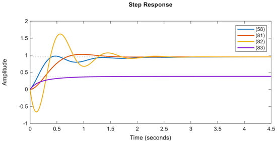
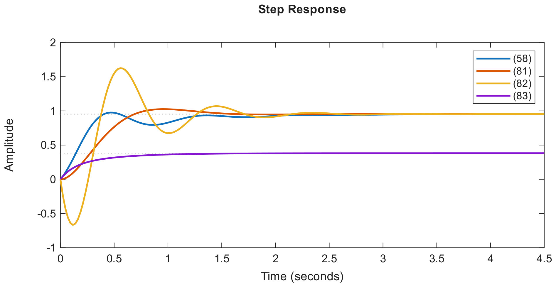
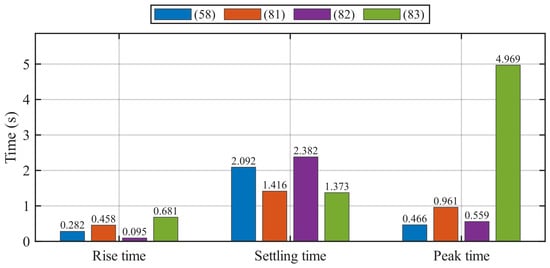
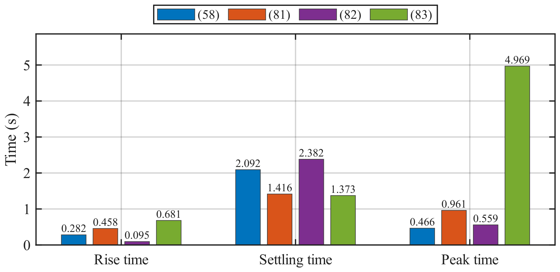
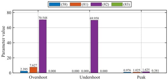
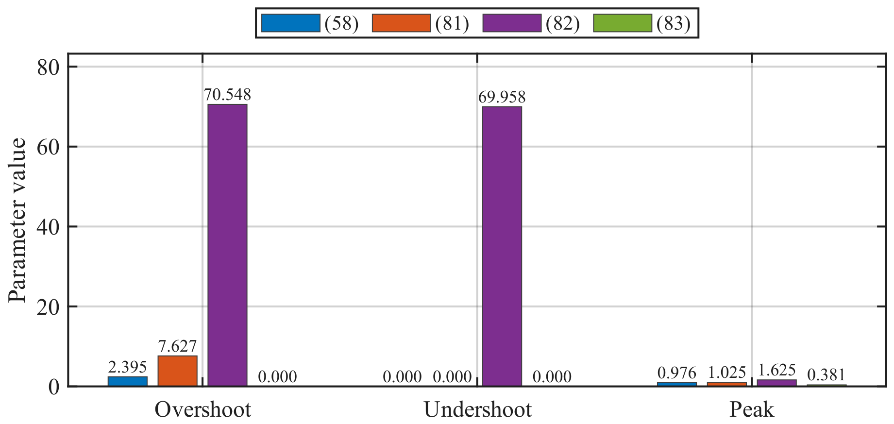
Figure 3 shows that the approximation follows the dominant step-response envelope, although it does not reproduce every fast oscillation of the fifth-order residual. Table 6 tabulates different time-domain measures obtained for responses plotted in Figure 3. These values are also plotted in Figure 4 and Figure 5 for comparison. According to Table 6, overshoot of the higher-order residual model, i.e., Equation (58), is 2.394529%, whereas the proposed model, i.e., Equation (81), gives an overshoot of 7.626725%. Thus, the absolute increase in overshoot is about 5.23 percentage points. However, the pole-retention model, i.e., Equation (82), gives a considerably larger overshoot of 70.548480% together with an undershoot of 69.957672%. Therefore, although the overshoot of the proposed model is higher than that of the original system, it is substantially lower than that obtained using the pole-retention method.

Figure 3. Step responses of the full-order residual and the reduced models.

Table 6. Time-domain measures for the full-order residual and reduced-order models.

Parameter	Equation (58)	Equation (81)	Equation (82)	Equation (83)
Rise time (s)	0.281901	0.458218	0.094970	0.681344
Settling time (s)	2.091649	1.415941	2.381871	1.373358
Overshoot (%)	2.394529	7.626725	70.548480	0
Undershoot (%)	0	0	69.957672	0
Peak	0.975662	1.025498	1.625065	0.381137
Peak time (s)	0.466260	0.961328	0.558883	4.968684

Figure 4. Comparison of rise time, settling time, and peak time.

Figure 5. Comparison of overshoot, undershoot, and peak magnitude.

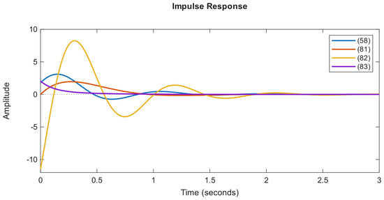
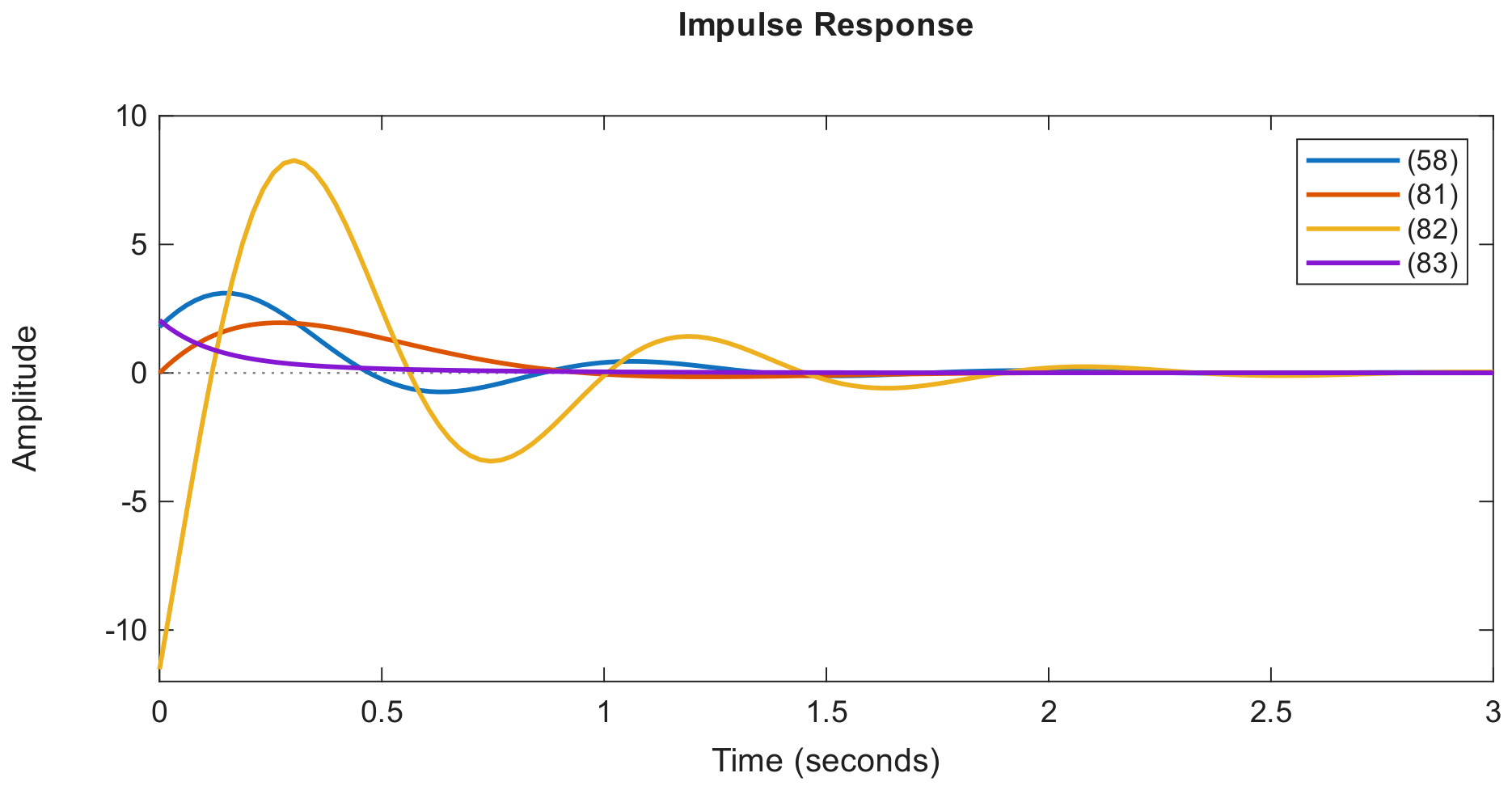
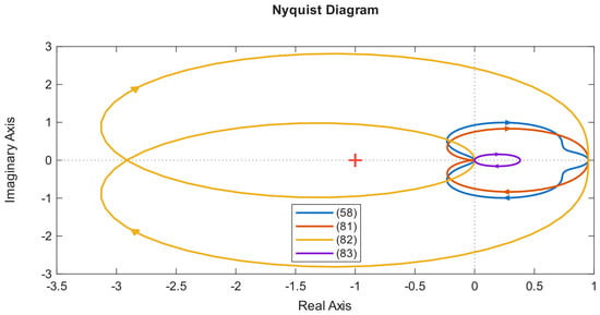
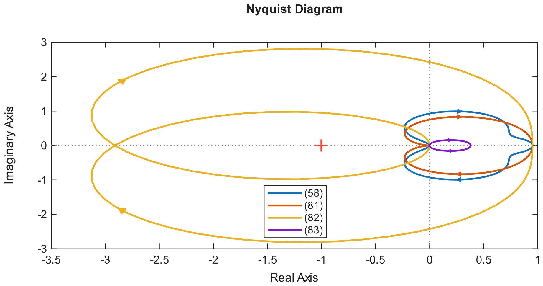
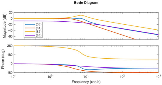
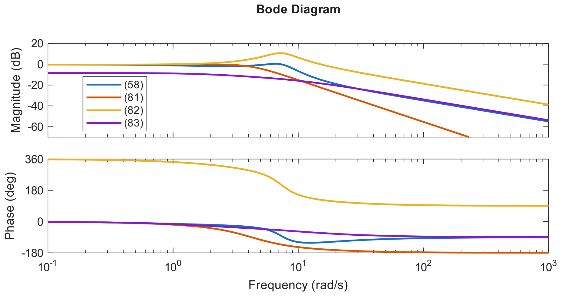
The impulse plot in Figure 6 leads to the same interpretation: the second-order model retains the principal decay pattern but smooths the rapid oscillatory content. In the frequency domain, Figure 7 and Figure 8 show good agreement in the low-frequency region most relevant to frequency-response studies. The curves separate at higher frequencies, where the discarded modes have a stronger influence. Neither Nyquist curve encircles the critical point, which is consistent with the pole-based stability check.

Figure 6. Impulse responses of the full-order residual and the reduced models.

Figure 7. Nyquist comparison of the full-order residual and the reduced models.

Figure 8. Bode comparison of the full-order residual and the reduced models.

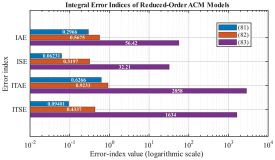
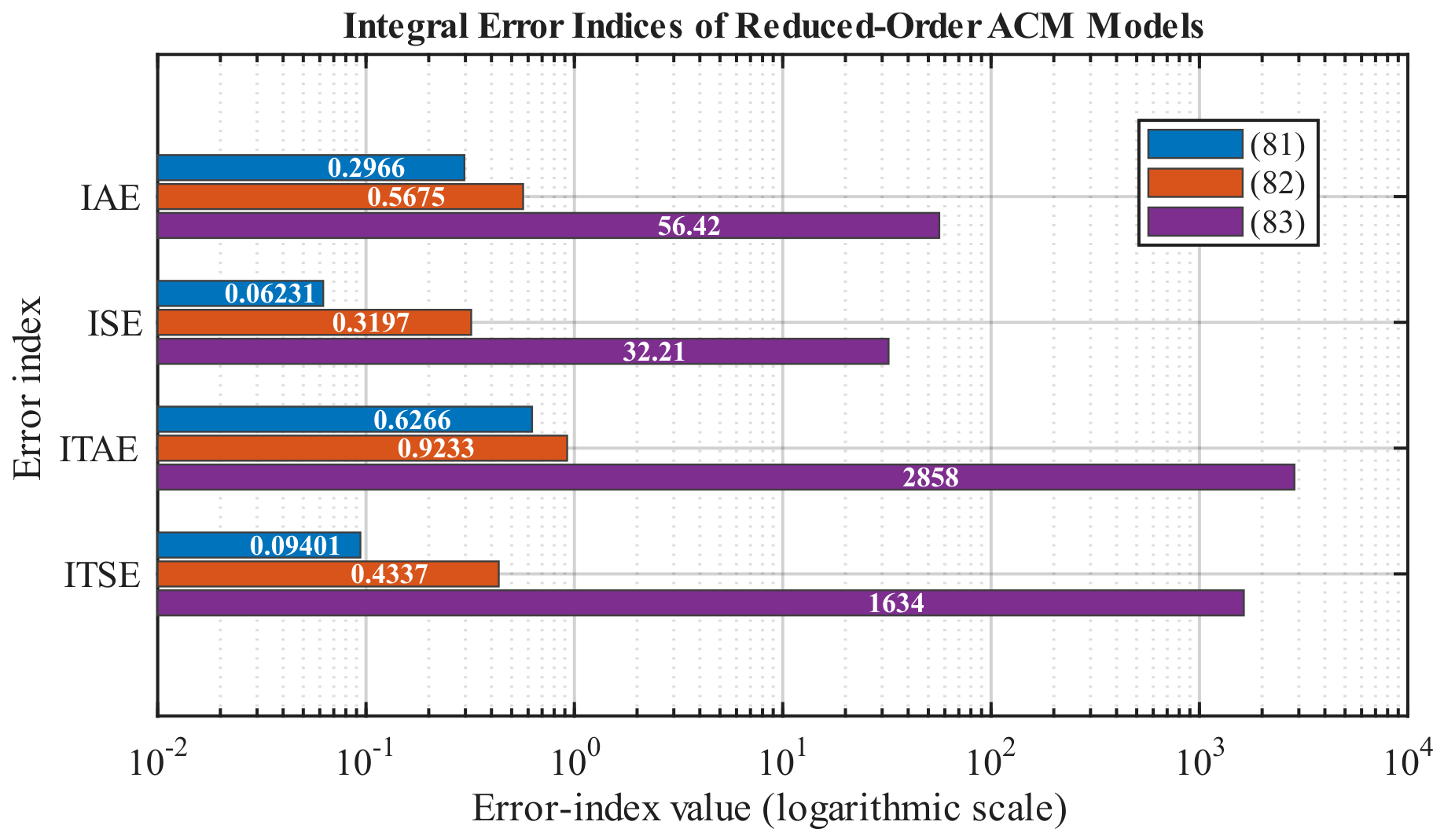
The accumulated response mismatch is summarized by the error measures in Table 7 and Figure 9. The proposed model, i.e., Equation (81), gives IAE, ISE, ITAE, and ITSE values of $0.29660$, $0.06231$, $0.62660$, and $0.09401$, respectively. These values are lower than the corresponding values obtained using the pole-retention model, i.e., Equation (82), for which IAE, ISE, ITAE, and ITSE are $0.5675$, $0.3197$, $0.9233$, and $0.4337$, respectively. The differentiation model, i.e., Equation (83), produces substantially larger error indices, with IAE, ISE, ITAE, and ITSE values of $56.42$, $32.21$, 2858, and 1634, respectively.

Table 7. Integral error indices for models.

Error Index	Equation (81)	Equation (82)	Equation (83)
IAE	0.29660	0.5675	56.42
ISE	0.06231	0.3197	32.21
ITAE	0.62660	0.9233	2858
ITSE	0.09401	0.4337	1634

Figure 9. Integral error indices for the reduced residual models.

Thus, the proposed AHP–BBOA model provides the minimum value of all four considered integral error indices among the reduced-order models. In particular, the small ISE and ITSE values of $0.06231$ and $0.09401$ indicate that large-amplitude and time-weighted squared errors are not sustained in the proposed approximation. The comparatively low IAE and ITAE values also show that the overall absolute response mismatch remains limited over the simulation interval. In contrast, the substantially higher error indices of the differentiation model indicate a considerably larger deviation from the higher-order residual dynamics.

Taken together, the pole locations, limiting gains, time- and frequency-domain responses, and integral error indices support the effectiveness of the proposed AHP–BBOA reduction. The resulting model is substantially simpler than the higher-order system, preserves the quantities imposed by the formulation, and provides a better overall approximation than the conventional pole-retention and differentiation models considered in this study.

7. Conclusions

Lower-order representations help in easier analysis, controller design, and repeated simulation studies. An AHP-BBOA framework is used to replace the fifth-order ACM dynamics with a stable second-order model in this contribution. The direct term is extracted before reduction. Then, AHP-weighted time-moment and Markov-parameter errors are used for framing the objective function. Thus, the framed objective function is utilised to derive the model under gain-matching and Hurwitz constraints. The final approximation preserves the feedthrough term exactly and matches the steady-state gain to within about $0.002\%$. Time- and frequency-domain results show that it more appropriately retains the dominant ACM behaviour compared to other conventional methods. The model is therefore a practical compact representation for frequency-response studies and controller development. Future work can address uncertain parameters, nonlinear operation, communication delays, hardware-in-the-loop validation, and other energy storage system applications [24].

References

- Waghmare, A.; Singh, V.; Varshney, T.; Sanjeevikumar, P. A systematic review of reinforcement learning-based control for microgrids: Trends, challenges, and emerging algorithms. Discov. Appl. Sci. 2025, 7, 939. [Google Scholar] [CrossRef] [Scilit]
- Samal, M.; Panigrahi, C.K.; Gupta, D.K. Load Frequency Control in Modern Power System-An Overview. In Proceedings of the 2025 International Conference on Power Electronics Converters for Transportation and Energy Applications (PECTEA), Jatni, India, 18–21 June 2025; IEEE: Piscataway, NJ, USA, 2025; pp. 1–6. [Google Scholar]
- Pati, S.S.; Subudhi, U.; Mishra, S. Robust Frequency Regulation Management System in a Renewable Hybrid Energy Network with Integrated Storage Solutions. Electricity 2025, 6, 22. [Google Scholar] [CrossRef] [Scilit]
- Sasidhar, P.R.S.; Gebremedhin, A.; Norheim, I. Multi-energy microgrid design and the role of coupling components—A review. Renew. Sustain. Energy Rev. 2025, 216, 115540. [Google Scholar] [CrossRef] [Scilit]
- Coelho, F.C.; Assis, F.A.; José Filho, C.C.; Donadon, A.R.; Roncolatto, R.A.; Andrade, V.E.; Rosas, P.A.; Barcelos, S.L.; Saavedra, O.R.; Bento, R.G.; et al. Monte Carlo simulation of community microgrid operation: Business prospects in the Brazilian regulatory framework. Util. Policy 2025, 92, 101856. [Google Scholar] [CrossRef] [Scilit]
- Apperley, M.; Viggers, H.; Walmsley, M.; Chapman, R.; Howden Chapman, P.; Penny, G.; Shearer, I.; Taptiklis, P. The role of smart community microgrids in Aotearoa’s energy future. J. R. Soc. N. Z. 2025, 55, 1147–1166. [Google Scholar] [CrossRef] [Scilit] [PubMed]
- Dabbaghjamanesh, M.; Senemmar, S.; Zhang, J. Resilient distribution networks considering mobile marine microgrids: A synergistic network approach. IEEE Trans. Ind. Inform. 2020, 17, 5742–5750. [Google Scholar] [CrossRef] [Scilit]
- Daraz, A. Optimized cascaded controller for frequency stabilization of marine microgrid system. Appl. Energy 2023, 350, 121774. [Google Scholar] [CrossRef] [Scilit]
- Huylo, M.; Taheri, S.; Novoselac, A. Integration of renewable energy generation and storage systems for emissions reduction in an islanded campus microgrid. Build. Environ. 2025, 274, 112736. [Google Scholar] [CrossRef] [Scilit]
- Woo, T.H.; Kim, Y.I. Microgrid control incorporated with Small Modular Reactor (SMR)-based power productions in the university campus. Prog. Nucl. Energy 2025, 183, 105678. [Google Scholar] [CrossRef] [Scilit]
- Singh, S.; Singh, V.; Mathur, A.; Bashishtha, T.; Padmanaban, S.; Varshney, T. Airport microgrid control using integral-of-absolute-error having high renewable penetration. Sci. Rep. 2025, 15, 23550. [Google Scholar] [CrossRef] [Scilit] [PubMed]
- Liaw, C.M.; Yang, C.W.; Jhou, P.H. Airport microgrid and its incorporated operations. Aerospace 2024, 11, 192. [Google Scholar] [CrossRef] [Scilit]
- Guo, S.; He, J.; Ma, K.; Yang, J.; Wang, Y.; Li, P. Robust economic dispatch for industrial microgrids with electric vehicle demand response. Renew. Energy 2025, 240, 122210. [Google Scholar] [CrossRef] [Scilit]
- Zhai, C.; Cao, Z.; Wang, Y.; Abdou-Tankari, M.; Yu, J.; Lei, Z. A reverse incentive-based demand response strategy for shared energy storage in industrial microgrids: Optimization, scheduling, and investment analysis. Energy 2025, 330, 136882. [Google Scholar] [CrossRef] [Scilit]
- Bashishtha, T.; Singh, V. Chien-hrones-reswick method-based pid control strategy for mitigation of frequency deviation of islanded microgrid. Electr. Eng. 2025, 107, 8085–8099. [Google Scholar] [CrossRef] [Scilit]
- Guo, Z.; Tang, Z. Hybrid Approach Based On Tensor Decomposition For Model Order Reduction Applied To Motor Diagnosis. IET Sci. Meas. Technol. 2026, 20, e70045. [Google Scholar] [CrossRef] [Scilit]
- De Parga, S.A.; Tezaur, R.; Hernández, C.G.; Farhat, C. Nonlinear projection-based model order reduction with machine learning regression for closure error modeling in the latent space. Comput. Methods Appl. Mech. Eng. 2026, 448, 118443. [Google Scholar] [CrossRef] [Scilit]
- Prakash, T.; Singh, P.P.; Singh, V.P.; Singh, S.N. A novel brown-bear optimization algorithm for solving economic dispatch problem. In Advanced Control & Optimization Paradigms for Energy System Operation and Management; River Publishers: Gistrup, Denmark, 2023; pp. 137–164. [Google Scholar]
- Shayeghi, H.; Davoudkhani, I.F.; Bizon, N. Robust self-adaptive fuzzy controller for load-frequency control of islanded airport microgrids considering electric aircraft energy storage and demand response. IET Renew. Power Gener. 2024, 18, 616–653. [Google Scholar] [CrossRef] [Scilit]
- Bashishtha, T.; Singh, V.; Yadav, U.; Varshney, T. Reaction curve-assisted rule-based pid control design for islanded microgrid. Energies 2024, 17, 1110. [Google Scholar] [CrossRef] [Scilit]
- Varshney, T.; Singh, V.; Dubey, K. Design of ISE-based frequency regulation scheme for airport microgrids using FOPDT approximation and reaction curve method. Sci. Rep. 2025, 16, 488. [Google Scholar] [CrossRef] [Scilit] [PubMed]
- Vu, N.K.; Nguyen, H.Q. Model order reduction algorithm based on preserving dominant poles. Int. J. Control. Autom. Syst. 2021, 19, 2047–2058. [Google Scholar] [CrossRef] [Scilit]
- Manohar, H.; Sambariya, D. Model order reduction of MIMO system using differentiation method. In Proceedings of the 2016 10th International Conference on Intelligent Systems and Control (ISCO), Coimbatore, India, 7–8 January 2016; IEEE: Piscataway, NJ, USA, 2016; pp. 1–5. [Google Scholar]
- Wang, K.; Cheng, L.; Yin, M.; Zhang, K.; Wang, R.; Zhang, M.; Sun, R. Evolutionary Game Theory in Energy Storage Systems: A Systematic Review of Collaborative Decision-Making, Operational Strategies, and Coordination Mechanisms for Renewable Energy Integration. Sustainability 2025, 17, 7400. [Google Scholar] [CrossRef] [Scilit]
Disclaimer/Publisher’s Note: The statements, opinions and data contained in all publications are solely those of the individual author(s) and contributor(s) and not of MDPI and/or the editor(s). MDPI and/or the editor(s) disclaim responsibility for any injury to people or property resulting from any ideas, methods, instructions or products referred to in the content. |
© 2026 by the authors. Licensee MDPI, Basel, Switzerland. This article is an open access article distributed under the terms and conditions of the Creative Commons Attribution (CC BY) license.