


Abstract
Dust accumulation has a substantial impact on photovoltaic (PV) power generation in desert environments, and soiling losses also cause significant operational difficulty for large-scale PV systems in desert countries like Saudi Arabia. This study describes a simulation-based approach for evaluating seasonal PV soiling losses and identifying the most economical cleaning interval for PV systems operating in desert conditions. The analysis was conducted as a literature-constrained, climate-informed scenario study representing Arar-like desert conditions using PVsyst and externally applied soiling assumptions. PV system performance was assessed under various cleaning scenarios, and seasonal soiling profiles were included as monthly loss factors based on desert environmental conditions. A nonlinear climate-informed scenario model incorporating wind speed and relative humidity was used to illustrate how these environmental drivers can be incorporated into the representation of dust adhesion and accumulation, while a Monte Carlo uncertainty analysis was employed to quantify the variability associated with the adopted seasonal soiling severity ranges and its effect on annual energy production. Under the base case economic assumptions, the 60-day interval produced the minimum total annual cost. Using a predefined near-optimality threshold of 1% above the minimum cost, the 90-day interval was also classified as a near-optimal operational alternative, resulting in a conditional base case range of 60–90 days. However, the sensitivity analysis reveals that the optimum is economically sensitive to the tariff and cleaning cost assumptions: under a high-power tariff, it moves to 45 days as the value of recovered energy grows; when the cleaning cost doubles, it moves to 90 days, as reducing maintenance frequency becomes more economically advantageous.
1. Introduction
Saudi Arabia has some of the world’s most substantial solar resources, yet desert conditions drive frequent soiling that can substantially reduce energy yield. In arid environments, soiling losses may dominate the operational loss budget when cleaning is infrequent; consequently, identifying a cleaning schedule that is both technically and economically optimal is a practical requirement for PV owners and developers. Soiling is commonly quantified by the soiling ratio (SR), defined as the ratio of power output (or irradiance response) of a soiled reference to a clean reference. Early utility-scale studies showed measurable energy losses attributable to soiling and emphasized the dependence on site conditions and maintenance practices. Recent sector reports synthesize standardized definitions and provide guidance for quantifying soiling losses at PV plants. In desert climates, wind and humidity strongly influence deposition and adhesion, and are among the most interactive variables governing soiling dynamics according to data-driven studies. In Saudi Arabia, dust events and aerosol loading can be severe, and multi-city analyses have included Arar as a location affected by major dust episodes. Arar’s northern desert location experiences distinct seasonal patterns with episodic dust storms, relatively low rainfall, and specific dust composition typical of the Arabian Peninsula. Soiling of surfaces with optical properties reduces energy yield and permanently degrades surface characteristics, decreasing light transmission and reflection [1]. These findings motivate a site-specific assessment that captures seasonal behavior and enables cleaning decisions grounded in quantified energy and cost impacts. As shown in [2], an insufficient soiling mitigation plan in high-solar-potential and soiling-prone countries such as China, India, and the Middle East can cancel out the significant development in solar cell and solar power system (CSP) efficiency made in recent decades in a few weeks. There is no one-size-fits-all solution to the soiling problem because of site-specific and seasonal fluctuations, variations in local energy prices, and the availability and cost of cleaning resources such as water or staff. This impact is amplified in areas without rainfall during peak solar summer months, such as California and the southwest region of the United States [3]; frequent cleaning can greatly increase energy generation and water consumption, prompting the development of water-saving and cost-effective soiling solutions. Elamim et al. [4] mentioned that, after 9 months of operation, the average efficiency of coated PV panels improves by roughly 10% compared to the reference system during the first three months (cleaning phase). The dust that collects on the ground contributes significantly to the loss of power from solar PV modules. Javed et al. [5] showed that dust storms reduced solar radiation reaching PV panels by 8% and increased annual average soiling rates by 23% compared to non-dust storm days. PV performance can also decrease from 2% to 50%, depending on the local environment and other factors [6]. Soiling losses in PV systems have been extensively researched for decades, as documented in several studies [7,8,9,10]; they can range from 5% to 50% of the system’s production, and can occur over six months or more [11]. As PV installation capacity grows, even little enhancements in the infrastructure and management of solar farms can result in a considerable boost in revenue [12], such as efficient reduction in accumulated dust on panels or soiling. To address the latter issue, researchers are exploring novel ways to reduce soiling and improve plant performance. For example, substantial efforts are being devoted to the creation of anti-soiling coatings, which can boost optical performance by up to 40% [13], and various cleaning techniques have been evaluated, such as dry, moist, and natural cleaning [14,15,16,17]. However, the problem with using these techniques lies in the lack of standardized measurement criteria and methods [18]. Other studies have extensively theorized that various forces are operating between the settled dust particles and the solar panels, causing them to stick together [19,20,21]. High-speed winds also have the potential to harm solar cells and shatter the base on which they are mounted, but low-speed winds contribute to removing dust from the solar cell surface, increasing PV panel productivity [22,23,24]. It has been discovered that dust settlement causes more particles to settle, resulting in greater dust accumulation on the surface of PV modules [25,26]. It has also been demonstrated that dust deposition and contaminants reduce solar cell productivity, and so PV panels must be cleaned on a regular basis to eliminate collected dust [27,28,29]. In the same context, soiling monitoring is one of the most prevalent approaches for measuring soiling rates at a specific location and scheduling ideal cleaning scenarios. Several strategies have been described in the scientific literature; for example, some researchers utilize optical measurements, exposing glass samples and quantifying the decrease in transmittance caused by dirt accumulation [19], while other technologies employ commercial soiling sensors such as Dust [30] and the MARS sensor [31], or low-cost sensors such as NREL’s DUSST sensor [32] or Figgis et al.’s microscopic setup [33]. Among these methods, the microfiber-based wiper and the microfiber and vacuum cleaner combination are the most effective cleaning techniques, with a weekly improvement of almost 6% over the control panel [34]. During high-soiling months, focused cleaning interventions raised PR by 10.28%, and temperature-corrected performance ratios improved by up to 8.77% [35]. A bi-weekly cleaning schedule during the dry season is the best option for our location in terms of energy efficiency compared to daily cleaning [36]. Of daily, weekly, and monthly cleaning frequencies, weekly cleaning is the most effective under the evaluated climate circumstances. Figure 1 illustrates the extent to which dust and deposits affect the performance of PV systems. Maintaining optimal PV performance requires a thorough grasp of the mechanics of dust collection in addition to efficient, situation-specific cleaning techniques [37]; to assess the economic impact of soiling on revenue and establish the most cost-effective time to physically clean a system, one must first understand the impact of soiling on system performance deterioration in terms of rate and severity [38]. These solutions increase energy output and improve the economic viability of solar energy, making it a more dependable and sustainable energy source in areas affected by dust-related performance degradation. The investigation underlines the importance of customized cleaning schedules, the use of appropriate cleaning procedures, and the incorporation of innovations such as AI-powered robotic cleaning equipment to increase the operation of photovoltaic solar energy systems.
Figure 1.
Photographs illustrate the experimental context of PV soiling. The (left) image shows PV modules installed at a solar testing facility, while the (right) image presents a dust-covered PV module before cleaning, demonstrating the typical surface contamination encountered in desert environments [34].
Although several studies have investigated PV soiling and cleaning optimization in Saudi Arabia, most have focused on region-specific economic analyses or fixed soiling assumptions without explicitly integrating environmental variability into the optimization framework. In addition, uncertainty associated with soiling behavior has rarely been quantified. To address these gaps, this study develops an integrated framework that combines PVsyst simulation, a nonlinear climate-dependent soiling accumulation model incorporating wind speed and relative humidity, Monte Carlo uncertainty analysis, and a conditional scenario-based cleaning analysis representing Arar-like desert conditions. This integrated methodology provides a more comprehensive basis for evaluating economically optimal PV cleaning strategies under desert environmental conditions. This research had the following aims: address the critical challenge of seasonal soiling rates; improve the cleaning processes for PV solar energy systems in the Saudi desert climate; optimize cleaning, enhance performance, and minimize maintenance costs using PVsyst simulation, specifically targeting Arar city in the northern border region; evaluate conditional alternative cleaning intervals under the adopted literature-constrained and economic assumptions that can be improved by understanding seasonal variation, thereby increasing the long-term, and even short-term, economic viability of large- and smaller-scale PV projects. This paper is organized as follows: the Case Study Site: Arar (Northern Border Province) Subsection and Section 2, Section 3, Section 4 and Section 5 present the case study site, materials and methods, data and tools, results and discussion, and conclusion, respectively.
Case Study Site: Arar (Northern Border Province)
Arar (30.98° N, 41.02° E) is located in Saudi Arabia’s Northern Border Province and has a typical arid desert climate with high solar irradiation, little annual precipitation, and frequent dust events. Long-term climatic records show that summer maximum temperatures frequently exceed 40–45 °C, while winter minimum temperatures typically range between 0 and 5 °C and may occasionally drop below freezing. The average annual precipitation is around 137 mm, with the majority of the rain falling in the winter and spring; the average yearly relative humidity is around 29%, ranging from 15% during the hot summer months to more than 50% in the winter. Wind speeds range from 6 to 8 m/s on average; however, dust storms caused by northwesterly Shamal winds can reach 15 m/s or more. Arar’s climatic circumstances make it an ideal desert location for studying seasonal soil accumulation and PV cleaning optimization.
2. Materials and Methods
2.1. PV System Modeling
The clean-reference PV system was simulated using PVsyst (version 8.0; PVsyst SA, Satigny, Switzerland) to model and analyze the impact of seasonal soiling rates on PV system performance, enabling the simulation of various cleaning frequencies and scenarios to maximize energy output while reducing operation and maintenance (O&M) costs. A grid-connected PV system was modeled in PVsyst using a commercially available PV module and inverter from the built-in component databases [39], and array layout, tilt/azimuth, inverter sizing ratio, thermal model parameters, and electrical losses (wiring, mismatch, ohmic) were configured according to best practices. PVsyst was used to generate the deterministic clean reference energy output of the modeled PV system. In this simulation, the PVsyst soiling loss parameter was set to 0%; therefore, the resulting time-step energy output, , contains the modeled optical, thermal, electrical, mismatch, wiring, inverter, and other system losses, but no soiling loss. The meteorological inputs used to generate the PVsyst clean reference output, and the NASA POWER variables used in the external soiling analysis constituted separate data streams and were not combined as duplicate inputs within the PVsyst simulation.
Accordingly, monthly soiling factors were not applied in PVsyst, and an additional nonlinear soiling correction was not carried out. Instead, a single external climate-dependent soiling model was used to transform into the corresponding soiled energy output, thereby preventing double counting of soiling losses. PVsyst employs a thermal loss model to estimate the PV cell temperature from the ambient temperature, incident irradiance, module efficiency, and heat transfer to the surroundings. The total heat loss coefficient comprises a constant component, , and a wind-dependent component, . For the free-standing-open-rack configuration adopted in this study, = 29 and = 0 /(m). The cell temperature is expressed in Equation (1).
where is the PV cell temperature (), is the ambient temperature (), is the dimensionless solar absorptance of the module, is the incident irradiance on the module plane (), is the dimensionless module efficiency, is the constant heat loss coefficient (), is the wind-dependent heat loss coefficient , and is the wind speed (). In the present simulation, , while the nominal module efficiency is 0.213.
2.2. Soiling Modeling
2.2.1. Literature-Constrained Seasonal Soiling Severity Scenario Inputs
No continuous month-resolved field measurements for PV soiling loss were available for Arar. Accordingly, the monthly ranges in Table 1 were treated as bounded, literature-constrained seasonal scenario inputs rather than measured or field-calibrated Arar values. Their magnitudes were constrained using Saudi field evidence from Rumah in the central region [11,40], broader Saudi observations [6], and field studies from comparable Arabian and dry-climate environments [5,34,41,42,43,44,45]. The closest available Saudi evidence is the K.A.CARE/SEC campaign at Rumah (25.571184° N, 47.151679° E), where two 12-module arrays—one regularly cleaned and one allowed to soil—were monitored during a three-year campaign. One-year analyses reported by Jones et al. [11] and Baras et al. [40] yielded representative soiling rates of approximately 0.210–0.233% day−1, equivalent to about 6.3–7.0% over a 30-day dry exposure before accounting for intervening natural or scheduled cleaning.
Table 1.
Adopted literature-constrained monthly soiling-severity scenario ranges used in the deterministic and uncertainty analyses. These ranges are scenario inputs and should not be interpreted as field-measured monthly soiling losses for Arar.
These monthly ranges were not applied as an additional loss to an already soiled PVsyst energy output. PVsyst was operated with soiling set to 0% to provide the clean reference energy series, while the monthly ranges were incorporated into the external soiling framework.
For month (m), the deterministic seasonal reference value was defined as the arithmetic midpoint in the below equation:
where and are the lower and upper bounds of the adopted monthly scenario range. The midpoint values are 4% for January, February, and December; 10% for March and May; 11% for April; 15% for June and July; 14% for August; 7.5% for September and October; and 6.5% for November. The lower winter ranges (3–5%) are consistent with lower-severity and more frequently naturally cleaned periods reported in dry climates [44,45]. The intermediate ranges (approximately 5–13%) are consistent with the 30-day-equivalent Rumah field rate and with monthly or dry-period observations from Morocco and Cyprus [40,43,44]. The upper ranges (11–18%) are consistent with measurements from Arabian desert in Qatar, where uncleaned monthly power losses of approximately 12–24% and an average monthly energy yield reduction of about 15% have been reported [34,41].
The transfer to Arar was not performed as a one-to-one substitution of measurements from another city. Instead, the cited studies were used to define a plausible bounded severity envelope and seasonal ordering, Arar-specific NASA POWER relative humidity and wind speed data were used as climate drivers in the external daily soiling rate model, and irradiance was used for irradiation-weighted loss calculations. Precipitation and dew-point temperature were retained only for general climate characterization and did not enter the numerical soiling calculation.
Differences in aerosol composition, rainfall, humidity, module tilt, exposure duration, and cleaning practice prevent the cited field values from being interpreted as direct Arar measurements. In the deterministic analysis, the scenario midpoint characterizes the month-specific severity. In the uncertainty analysis, the complete lower and upper bounds are retained and converted into bounded monthly multipliers. Therefore, the monthly ranges and the nonlinear climate-dependent formulation represent complementary components of a single external soiling calculation rather than two independent loss factors applied sequentially to the PV energy output.
2.2.2. Mathematical Formulation of PV Soiling Losses
The soiling ratio (SR), shown in Equation (3), is defined as the ratio of the power output (P) of a soiled PV module to that expected of the same module if it were clean.
The instantaneous soiling loss (SL) is the fraction of energy lost due to soiling, calculated in Equation (4).
Annual energy loss due to soiling describes the change in soiling ratio over time, generally stated as a daily percentage loss, and is calculated by Equation (5), where is clean energy production.
The corresponding annual cost of energy loss is presented in Equation (6), which expresses the economic impact of an electrical system’s inefficiency through three primary components: τ, which is the electricity tariff (SAR/kWh); , which is the annual cost of energy loss, commonly represented in Saudi Riyals (SAR); and , which is the total annual energy loss, calculated as the sum of all energy dissipated during a year and measured in kilowatt-hours (kWh).
2.2.3. Nonlinear Soiling Accumulation Model
To represent the potential influence of environmental variability on soiling accumulation, the numerical workflow directly calculates a climate-informed daily soiling rate from relative humidity and wind speed. It does not calculate an intermediate deposited dust mass from airborne particle concentration or deposition velocity, as these variables were not available and were not used in the analysis. The implemented formulation is therefore an illustrative soiling rate scenario model rather than a particle-deposition model. A practical formulation for the daily soiling accumulation rate is presented in Equation (7).
Equation (7) is used in this study as an illustrative climate-informed scenario model to represent the qualitative dependence of daily soiling accumulation on relative humidity and wind speed. It is not presented as a field-calibrated or experimentally validated predictive model for Arar. Here, RH is relative humidity (fraction), WS is wind speed (m/s), and (k0) is the baseline scenario soiling rate coefficient (k0 = 0.00025 day−1). The parameters (β = 1.8) and (γ = 0.08 (m/s)−1) control the assumed sensitivity to humidity-related adhesion and wind-related removal/transport, respectively, while (RHref = 0.30) and (WSref = 4 m/s) define reference environmental conditions.
The numerical values of k0, β, γ, and WSref are fixed scenario parameters adopted for the present analysis; they were not obtained by fitting Equation (7) to Arar soiling ratio data. Consequently, coefficient-specific goodness-of-fit metrics and field-derived parameter confidence intervals are not reported. (RHref = 0.30) is used as a site-normalization reference and is close to the approximately 29% long-term annual relative humidity adopted for Arar. Published desert observations [5] support the physical motivation and qualitative direction of the environmental dependencies represented in Equation (7), including the influence of humidity, wind-driven resuspension/removal, and dust events on PV soiling. However, these observations are not used here as independent validation of the specific numerical coefficients. Accordingly, Equation (7) should be interpreted as a scenario analysis mechanism for incorporating climate dependence into the external soiling framework rather than as a validated site-specific predictive equation. Independent field measurements of the soiling ratio in Arar would be required to calibrate these coefficients and quantify parameter uncertainty and goodness of fit.
Assuming an approximately linear build-up between cleaning events, the average loss over a cleaning interval can be approximated using Equation (8).
is the average daily accumulation rate over the interval and T is the cleaning interval in days. This provides the deterministic climate-dependent basis for the external soiling calculation and links the environmental drivers to the adopted month-specific seasonal severity without introducing a second independent soiling loss term.
2.3. Cleaning Optimization Model
Cleaning optimization is formulated to minimize the total annual cost, composed of cleaning costs and energy loss cost as shown in Equation (9). For the 365-day (no planned cleaning) scenario, = 0, since no scheduled cleaning is performed during the year; therefore, the annual cleaning cost is zero, and the total annual cost consists only of the lost energy cost.
is the number of cleaning events per year based on the interval, T (days), and is the cost per cleaning event (SAR/kWp or SAR per plant, depending on scale). For the scheduled cleaning scenarios, the annual number of cleaning events was determined explicitly using a calendar-based integer schedule rather than the fractional approximation 365/T. The PV system was assumed to start the year in a clean condition. For a cleaning interval T < 365, scheduled cleaning events were performed on days (T, 2T, 3T, …, nT), provided that nT < 365. Accordingly,
This rule gives 12, 8, 6, 4, 3, and 2 scheduled cleaning events per year for the 30-, 45-, 60-, 90-, 120-, and 180-day scenarios, respectively. The 365-day case was explicitly defined as a no-planned-cleaning scenario with ( = 0). Annual cleaning cost was then calculated as shown in Equation (11).
The base case electricity value was set to = 0.14 SAR/kWh as a scenario parameter for monetizing soiling-related energy loss, rather than as a regulated national tariff or project-specific power-purchase-agreement price. This value lies within the range of electricity export values previously evaluated in a Saudi PV economic study, which examined values from 0.07 to 0.25 SAR/kWh and identified 0.14 SAR/kWh as an economic feasibility threshold [46]. Because the applicable value of recovered PV energy depends on project-specific contractual and market conditions, the influence of this assumption on the optimal cleaning interval was evaluated through economic sensitivity analysis. Therefore, no fractional cleaning events were used in the economic analysis. The base case cleaning cost was set to .80 SAR/kWp per scheduled cleaning event. This value is treated as a scenario-based unit-cost assumption rather than as a field-measured cleaning quotation for Arar. Actual cleaning expenditure may include labor, water, transportation, equipment operation, supervision, and other site-dependent overheads, and can vary with plant size, cleaning technology, water availability, and contractual arrangements. Published PV cleaning-optimization studies confirm that cleaning cost is a project-specific economic input and materially affects the optimal cleaning schedule [11,47]. Alvarez et al. [47], for example, evaluated baseline and technology-dependent cleaning costs in their economic analysis. The value adopted in the present study is not claimed to be directly derived from that study; instead, its influence is evaluated through the economic sensitivity analysis. An Arar-specific cost survey or contractor quotation would be required before applying the resulting interval to an actual project. In the present scenario model, each scheduled cleaning event is assumed to completely restore the modeled soiling state to the clean reference condition (SL = 0) immediately after cleaning, after which soiling accumulation restarts for the subsequent interval. Residual post-cleaning soiling and variations in cleaning efficiency are not explicitly modeled because no Arar-specific post-cleaning field measurements are available. Therefore, complete restoration is treated as an idealized modeling assumption rather than field-validated cleaning efficiency. The optimal interval T* is obtained by minimizing the total annual cost as illustrated in Equation (12a). The relative cost gap is calculated using Equation (12b).
where T denotes one of the evaluated cleaning intervals (30, 45, 60, 90, 120, 180, or 365 days); is the total annual cost associated with cleaning interval T; is the minimum total annual cost among the evaluated intervals; and is the percentage by which the total cost of interval T exceeds . In this study, an interval is classified as near optimal when . The 1% threshold is adopted as a transparent operational decision rule for distinguishing the cost-minimizing solution from economically close alternatives; it is not presented as a universal industry standard.
Monte Carlo Uncertainty Analysis
A Monte Carlo simulation with M = 10,000 realizations was used to propagate the uncertainty associated with the adopted monthly soiling severity. Rather than introducing an undocumented global Gaussian uncertainty for the soiling rate, the stochastic variation was derived directly from the lower and upper monthly soiling loss ranges adopted in this study. For month m, let Lm and Um denote the lower and upper bounds of the monthly soiling loss range, respectively, and let Mm = (Lm + Um)/2 denote the deterministic midpoint used in the soiling model. A dimensionless monthly multiplier was sampled from the bounded uniform distribution in Equation (13a).
One multiplier was sampled independently for each of the twelve calendar months in every Monte Carlo realization. The sampled value was held constant for all daily time steps belonging to the corresponding month. The monthly multipliers were assumed to be mutually independent across months and independent across Monte Carlo realizations. No temporal or cross-month correlation was imposed because no site-specific measurements were available to estimate such a dependence structure. The climate-dependent soiling rate in realization s was calculated by Equation (13b).
Therefore, σk is not introduced as an independently assumed global constant. Instead, its equivalent month-specific uncertainty is derived directly from the adopted bounds. For a uniform distribution, the equivalent standard deviation of the month-specific stochastic multiplier is calculated using Equation (14a), while the corresponding standard deviation of the sampled soiling rate is obtained from Equation (14b):
where Lm, Um, and Mm denote the lower bound, upper bound, and deterministic midpoint of the soiling loss range for month m, respectively; is the standard deviation of the dimensionless monthly multiplier; is the deterministic climate-dependent soiling rate at time step i; and is the corresponding month-specific standard deviation of the soiling rate.
Based on the monthly ranges adopted in this study, σr,m is 0.1443 for January, February, and December; 0.1155 for March, May, June, July, September, and October; 0.1050 for April; 0.1237 for August; and 0.1332 for November. No independent stochastic perturbation was applied to the baseline energy output because no site-specific field measurements were available to estimate an independent energy model uncertainty. Accordingly, σE was set to zero, and the Monte Carlo spread reported in this study represents uncertainty associated specifically with the adopted soiling ranges. This treatment avoids introducing an arbitrary energy model uncertainty and is consistent with the site-dependent treatment of uncertainty discussed in PVsyst documentation [48] and with the importance of explicitly accounting for soiling variability in long-term PV performance forecasting [49].
Table 1 shows that the numerical bounds are supported as a combined literature envelope. Rumah provides the nearest Saudi dry desert field benchmark, with representative rates of approximately 0.210–0.233% day−1, corresponding to about 6.3–7.0% per 30 dry days [11,40]. Qatar provides the strongest evidence from Arabian deserts for the upper monthly range, with reported losses of approximately 12–24% during an uncleaned month and an average monthly energy yield reduction of about 15% [34,41]. Measurements from Morocco indicate PV soiling rates of approximately 0.083–0.36% day−1, corresponding to approximately 2.5–10.8% over 30 dry days [43]. The Cyprus study reported monthly soiling loss indices ranging from 0.30% to 4.34%, with higher deposition rates during dust events [44]. These field observations support the magnitude of the adopted bounds but do not constitute month-specific measurements for Arar.
The only stochastic inputs in the Monte Carlo analysis are the 12 monthly dimensionless multipliers . The climate-dependent model parameters, , β, γ, RHref, and WSref, as well as the clean reference energy series, are held fixed in all realizations.
Table 2 consolidates the fixed parameters, stochastic inputs, sampling assumptions, and clean reference conditions used in the Monte Carlo analysis. By distinguishing the sampled quantities from the parameters held fixed across all realizations, the table provides a transparent and reproducible definition of the uncertainty analysis framework.
Table 2.
Fixed and stochastic inputs used in the uncertainty analysis.
For each Monte Carlo realization, the sampled climate-dependent soiling rates are accumulated between two consecutive cleaning events to obtain the cumulative soiling load, , as expressed in Equation (15):
where is the cumulative soiling load up to time step n in realization s, is the sampled soiling rate, and is the time-step duration. The accumulated soiling state was reset to zero immediately after every scheduled cleaning event, representing complete restoration to the clean condition.
Because is defined as a fractional daily soiling loss rate, its time integral is dimensionless. Therefore, no additional empirical conversion coefficient is required. Because the stochastic variability is already introduced through the bounded monthly multiplier and propagated through and , no additional Gaussian perturbation was applied to either the soiling rate or the baseline energy output. The realization-specific soiling transmittance factor was calculated directly from the accumulated dimensionless soiling load using Equation (16).
The corresponding soiled energy output for each realization was then calculated directly from the deterministic clean energy output and the realization-specific soiling transmittance factor by using Equation (17):
where is the baseline clean-energy output at time step n, and is the corresponding soiled energy output in realization s. No stochastic perturbation was applied to . Consequently, = 0, and the uncertainty interval reported in this study represents only the uncertainty propagated from the adopted monthly soiling severity ranges. For each realization, the annual relative soiling-related energy loss was calculated by comparing the annual soiled energy output with the corresponding clean reference energy output using Equation (18):
The ensemble mean and standard deviation of the annual relative loss were subsequently calculated over the M = 10,000 Monte Carlo realizations using Equations (19) and (20), respectively:
The climate-informed stochastic model was used to quantify the relative response of annual soiling loss to the adopted monthly uncertainty ranges rather than to independently replace the deterministic energy-loss result. For each realization, a dimensionless uncertainty-response factor was calculated by Equation (21).
where is the irradiation-weighted relative loss obtained in realization s, and is the corresponding loss obtained using the deterministic monthly multipliers = 1. The irradiation weighting was derived from the hourly NASA POWER for 2016–2025, aggregated to daily irradiation values consistently with the daily soiling rate formulation. The 24 unavailable irradiation records from 31 December 2025 were excluded from the irradiation-weighted aggregation; all relative humidity and wind speed records were complete. The annual realization-specific energy loss was subsequently calculated using Equation (22).
where = 84 kWh/kWp is the deterministic annual soiling-related energy loss obtained for the 60-day cleaning strategy. This two-stage formulation preserves the deterministic energy baseline while propagating the relative uncertainty associated with the adopted monthly soiling severity ranges and climate-dependent accumulation model. Accordingly, the stochastic model is interpreted as an uncertainty propagation layer rather than an independent predictor of absolute energy.
The uncertainty analysis was implemented using 10,000 independent Monte Carlo realizations. A fixed pseudorandom seed of 2026 was used solely to ensure numerical repeatability of the random sampling sequence. For each realization, the sampled monthly soiling multipliers were propagated through the same soiling accumulation and energy loss calculations used in the deterministic analysis, producing one dimensionless uncertainty response factor , which was subsequently applied to the deterministic 60-day loss baseline using Equation (22).
The resulting 10,000 conditional annual loss values, , were sorted in ascending order. P10loss, P50loss, and P90loss were then defined as the empirical 10th, 50th, and 90th percentiles of the ordered conditional loss ensemble, respectively.
Because the reported variable is energy loss, P10loss represents the lower-loss percentile and P90loss represents the higher-loss percentile. These loss percentiles should not be confused with the conventional PV industry probability-of-exceedance notation for energy yield, in which P90 yield represents a conservative production level expected to be exceeded with 90% probability [48,49]. Monte Carlo convergence was assessed using nested ensemble sizes of 1000, 2500, 5000, and 10,000 realizations generated from the same pseudorandom sequence using the fixed seed of 2026. Numerical stability was evaluated by comparing the mean, P10loss, P50loss, and P90loss estimates between 5000 and 10,000 realizations. A relative change below 0.5% was adopted as the numerical stability criterion. The principal technical specifications and simulation assumptions adopted for the PVsyst clean reference model are summarized in Appendix A, Table A1. The modeled system is a 999.9 kWp grid-connected, fixed-tilt, free-standing PV system located in Arar, Saudi Arabia, with a south-facing tilt angle of 25° and a nominal AC capacity of 900 kW. PVsyst was operated with the soiling loss parameter set to 0% to generate the clean reference energy series.
3. Data and Tools
Two meteorological data streams were used for separate components of the analysis. First, the clean reference energy series, was generated in PVsyst using a Meteonorm-based synthetic hourly meteorological file for Arar. The PVsyst soiling loss parameter was set to 0%; consequently, this simulation provided the reference PV energy output before the application of the external soiling model. The Meteonorm file represents a synthetic reference meteorological year generated from long-term monthly climatic statistics and should not be interpreted as an observed hourly record covering 2016–2025 [39].
Second, an independent NASA POWER hourly dataset was retrieved for Arar at 30.98° N, 41.02° E, covering 1 January 2016 to 31 December 2025 [50]. The retrieved variables were global horizontal irradiance (ALLSKY_SFC_SW_DWN), ambient temperature (T2M), relative humidity (RH2M), wind speed at 10 m (WS10M), corrected precipitation (PRECTOTCORR), and dew point temperature (T2MDEW). These data were not used to impose a second set of meteorological losses within PVsyst. Instead, they were processed independently for the external climate-informed soiling analysis, irradiation-weighted temporal aggregation, and general climate characterization.
The hourly relative humidity and wind speed records were aggregated to daily mean values to match the daily time step of the soiling accumulation model. Relative humidity was converted from percent to fractional form before use in Equation (7). Hourly irradiance was aggregated to daily irradiation for the irradiation-weighted loss calculations. For the monthly visualization in Figure 2, the daily relative humidity and wind speed values were averaged by calendar month across the 2016–2025 period, while monthly mean daily GHI was calculated from the daily irradiation totals. The 24 unavailable GHI records from 31 December 2025 were excluded before aggregation. Precipitation and dew point temperatures were retained only for general climate characterization and were not used as numerical inputs to Equation (7), as natural cleaning thresholds, or as independently imposed soiling loss terms. The exact source, period, resolution, preprocessing, and analytical role of each variable are summarized in Table 3.
Figure 2.
Monthly mean relative humidity, mean daily global horizontal irradiation (GHI), and mean wind speed at 10 m in Arar based on the NASA POWER hourly dataset for 2016–2025. Relative humidity is represented by the red bars and referenced to the left vertical axis, whereas GHI and wind speed are represented by the brown and black bars, respectively, and referenced to the right vertical axis.
Table 3.
Data flow for the meteorological and energy variables used in the PVsyst clean reference simulation and the external climate-informed soiling analysis.
Figure 2, Figure 3 and Figure 4 present the NASA POWER variables that directly support the documented analysis. Figure 2 presents the long-term monthly mean relative humidity, mean daily global horizontal irradiation, and mean wind speed at 10 m, allowing their seasonal variations to be compared using clearly differentiated bar colors and explicitly labeled vertical axes. Figure 3 and Figure 4 present the hourly and monthly solar resource profiles, respectively. In the external soiling framework, daily relative humidity and wind speed enter the climate-dependent soiling rate formulation in Equation (7), while aggregated irradiance is used in the irradiation-weighted loss calculation. No independently derived dust risk index is used in the numerical workflow. NASA POWER was used as the source of the 2016–2025 meteorological variables employed in the external analysis and was not used as a source of empirical PV soiling loss measurements. The monthly soiling severity bounds were derived separately from the field studies cited in Section 2.2.1. The Global Solar Atlas was consulted only for general contextual verification of the regional solar resource and was not used as a numerical input to either the PVsyst simulation or the external soiling model.
Figure 3.
Average hourly distribution of global horizontal irradiance (GHI) throughout the year for Arar, illustrating the seasonal variation in solar resource availability used in the PV performance simulations.
Figure 4.
Monthly solar resource profile for Arar based on hourly meteorological data from 2016 to 2025, demonstrating the long-term seasonal consistency of solar irradiance used in this study.
Seasonal Soiling Loss Profile
Table 1 provides seasonal range inputs for Saudi desert conditions that can be used as PVsyst monthly loss inputs. For the Arar case study, summer and spring are typically assigned higher losses due to dust activity. Furthermore, dust originates from a variety of sources and is carried to various locations around Saudi Arabia, and dust storms have a significant impact on regional climate due to dust aerosols. The existence of dust particles in the atmosphere has a direct impact on the energy budget via absorption and dispersion.
4. Results and Discussion
The results were derived from the clean PVsyst reference yield (soiling = 0%) followed by a single external soiling calculation. The external model combines the nonlinear climate-dependent accumulation rate with the adopted monthly Arar seasonal severity inputs and explicitly resets the accumulated soiling state at each scheduled cleaning event. Therefore, the monthly seasonal ranges and the humidity/wind-dependent nonlinear formulation are not applied as separate sequential losses, and no double counting of soiling is introduced.
The normalized clean specific yield is 2120 kWh/kWp·year for a fixed-tilt utility-scale PV facility in Arar, and the monthly soiling inputs correspond to region-specific ranges, with the greatest losses occurring in the spring and summer months. Moreover, the economic assumptions for the base case are tariff = 0.14 SAR/kWh and cleaning cost = 1.80 SAR/kWp per cleaning event. The scenario outputs are presented on a specific-yield basis (per kWp), allowing them to be scaled for any plant size.
Table 4 shows the complete numerical result set for the primary cleaning situations. The lowest overall annual cost occurs at a 60-day interval, although the cost at 90 days is still quite close economically and thus defensible for operators who prioritize fewer cleaning interventions. Table 4 shows that introducing a 90-day scheduled cleaning strategy instead of the 365-day (no planned cleaning) case reduces the annual specific energy loss from 322 to 111 kWh/kWp, corresponding to a 65.5% reduction in soiling-related energy loss. Furthermore, the 60-day strategy decreases annual specific loss to 84 kWh/kWp, a 73.9% reduction compared to the uncleaned instance and a 24.3% improvement over the 90-day method. Although the 30-day strategy has the lowest energy loss, its cleaning costs were very high; thus, it is not the most cost-effective under base case economic assumptions. The minimum cost is attained at 60 days with a total yearly cost of 22.56 SAR/kWp·year, whereas the 90-day scenario offers 22.74 SAR/kWp·year. The base case optimum is 60 days, while 45 and 90 days become optimal under high-tariff conditions and when cleaning costs double, respectively. These results demonstrate how PV system performance is very sensitive to maintenance scheduling in arid climates, and that an improved cleaning approach can greatly reduce energy losses caused by soiling while still being economically viable. As a result, the suggested interval offers a workable compromise between energy yield preservation and operating costs, providing a solid framework for large-scale PV plant operation in arid areas.
Table 4.
Deterministic simulation results for the evaluated cleaning intervals, including integer cleaning events, annual energy loss, lost energy cost, cleaning cost, total annual cost, and the relative cost gap above the minimum total annual cost. Note: The relative cost gap was calculated using Equation (12b), where = 22.56 SAR/kWp·year at the 60-day interval. Intervals with were classified as near-optimal under the adopted base case assumptions.
Under the base case assumptions, the unique minimum total annual cost occurs at the 60-day interval, at 22.56 SAR/kWp·year. The 90-day strategy results in 22.74 SAR/kWp·year, an absolute increase of 0.18 SAR/kWp·year and a relative cost gap of approximately 0.80%. It therefore satisfies the predefined 1% near-optimality criterion. In contrast, the 45-day strategy costs 23.08 SAR/kWp·year, approximately 2.30% above the minimum, and does not satisfy the base case near-optimality criterion. Accordingly, 60 days is identified as the base case cost-minimizing interval, while 60–90 days represents the base case near-optimal operating range under the adopted assumptions.
The energy loss curve in Figure 5 increases monotonically as the cleaning interval increases, and steepens significantly after 90 days, showing that long intervals subject the plant to disproportionate summer dust collection. This pattern suggests using a more conservative cleaning interval once the schedule exceeds about one quarter.
Figure 5.
Annual specific energy loss as a function of the cleaning interval. The figure illustrates the nonlinear increase in energy losses as cleaning becomes less frequent under the adopted seasonal soiling profile.
The total cost curve in Figure 6 is convex because one cost component decreases while the other increases: frequent cleaning lowers lost energy costs while increasing direct O&M spending, whereas infrequent cleaning produces the opposite effect. The two curves are most successfully balanced at 60 days, with 90 days being approximately similar in practice.
Figure 6.
Annual cost components as a function of the cleaning interval in Arar. The total annual cost (blue) is the sum of the lost energy cost (green) and the cleaning cost (orange). The economically optimal interval is 60 days.
The uncertainty analysis for the 60-day strategy yields shows that, even when seasonal soiling severity is unclear, this scenario remains within a technically acceptable loss band, making it suitable for planning. Recovered energy is displayed against yearly cost savings in comparison to the no-cleaning scenario in Figure 7, where the cleaning is reframed as an investment in energy recovery and the energy recovered and annual cost averted are shown for each point. The 60-day scenario recovers over 74% of soiling losses and saves approximately 22.5 SAR/kWp·year and is therefore among the most effective and sensible choices.
Figure 7.
Recovery efficiency map showing the relationship between recovered soiling losses (%) and annual cost savings (SAR/kWp·year) relative to the no-planned-cleaning (365-day) scenario for each evaluated cleaning strategy. Annual cost savings were calculated as the difference between the total annual cost of each strategy and the no-planned-cleaning case (45.08 SAR/kWp·year). The 60-day scenario recovers over 74% of soiling losses and saves approximately 22.5 SAR/kWp·year.
In Figure 8, cleaning cost and annual loss are utilized to divide the cleaning strategies into operational zones, enabling the classification of tactics as economically weak, balanced, low-maintenance/high-loss, or high-performance. The strategies that are closest to the balanced-choice zone are the 60- and 90-day ones; longer intervals save cleaning time but also cause a disproportionate amount of energy loss for the plant.
Figure 8.
Graph classifying the evaluated cleaning strategies according to annual energy loss (kWh/kWp) and cleaning cost (SAR/kWp·year). Dashed lines indicate reference thresholds of 100 kWh/kWp for energy loss and 10.0 SAR/kWp·year for cleaning cost. Strategies in the bottom-right quadrant represent economically balanced and high-performance options. The values in parentheses represent the coordinates of each cleaning strategy, where the first value denotes the annual cleaning cost (SAR/kWp·year) and the second value denotes the corresponding annual energy loss (kWh/kWp). The 60- and 90-day strategies lie within the balanced operation region.
Figure 9 shows the combination of yield retention and total annual cost to distinguish the mathematical cost minimum from economically close operating alternatives. The 60-day strategy is the unique base case cost-minimizing solution. The 90-day strategy lies 0.80% above the minimum and therefore satisfies the predefined 1% near-optimality criterion. Consequently, the shaded 60–90-day region should be interpreted as a base case near-optimal operating range, not as evidence that both intervals are mathematically identical or universally optimal.
Figure 9.
Yield retention and total annual cost as functions of the cleaning interval. The 60-day interval is the base case cost-minimizing solution. The shaded 60–90-day region represents the base case near-optimal operating range defined by . The 90-day strategy costs 0.80% more than the minimum while reducing the required number of scheduled cleaning events from six to four per year.
Table 5 presents a scenario sensitivity analysis showing how the cost-minimizing cleaning interval changes under alternative electricity value and cleaning cost assumptions.
Table 5.
Scenario sensitivity analysis shows the influence of the assumed electricity value and cleaning cost on the cost-minimizing cleaning interval and corresponding minimum total annual cost.
The scenario sensitivity analysis shows that increasing the assumed electricity value from 0.14 to 0.25 SAR/kWh shifts the cost-minimizing interval from 60 to 45 days, with a minimum total annual cost of 29.90 SAR/kWp·year, because the higher economic value of lost energy makes more frequent cleaning favorable. Conversely, doubling the assumed cleaning cost from 1.80 to 3.60 SAR/kWp per event shifts the cost-minimizing interval from 60 to 90 days, with a minimum total annual cost of 29.94 SAR/kWp·year, because less frequent cleaning becomes economically preferable. Under the base case assumptions, 60 days is the unique cost-minimizing interval, while the 90-day strategy satisfies the predefined 1% near-optimality criterion. Therefore, the 60–90-day interval is interpreted as a conditional base case near-optimal operating range. Across the three evaluated economic scenarios, the cost-minimizing interval ranges from 45 to 90 days.
The completed scenario study for Arar reveals a significant nonlinear increase in annual soiling-related energy loss as cleaning intervals are extended. In terms of specific yield, annual energy loss increased from 45 kWh/kWp at a 30-day cleaning interval to 322 kWh/kWp when no regular cleaning was performed over the year, demonstrating that lengthy dust deposition in the northern Saudi desert can devour a large portion of potential yield if corrective cleaning is delayed. The economic trade-off between lost energy cost and direct cleaning expense resulted in a convex annual cost curve. Under the base case assumptions of 0.14 SAR/kWh electricity value and 1.80 SAR/kWp per cleaning event, the minimum total annual cost was achieved at a 60-day cleaning interval, equivalent to 22.56 SAR/kWp·year; the 90-day interval remained fairly close at 22.74 SAR/kWp·year, showing that the base case optimum is 60 days. However, sensitivity analysis indicates that the economically preferred interval may shift between 45 and 90 days depending on electricity tariff and cleaning cost assumptions (see Table 5). Specifically, when the tariff increased to 0.25 SAR/kWh, the optimum shifted from 60 days to 45 days since the value of recovered energy outweighed the additional cleaning cost; when the cleaning cost was doubled, the optimum changed to 90 days, indicating that the ideal interval is economically elastic and should be chosen based on project-specific income and O&M conditions. The deterministic 60-day cleaning scenario resulted in an annual soiling-related energy loss of 84 kWh/kWp. The deterministic annual loss of 84 kWh/kWp was used as the baseline for the uncertainty propagation analysis. The corresponding 10,000-realization Monte Carlo results are presented in Table 6.
Table 6.
Conditional Monte Carlo annual soiling loss results for cleaning strategy.
The Monte Carlo simulation yielded a conditional median loss (P50loss) of 83.942 kWh/kWp, with P10loss and P90loss values of 79.507 and 88.343 kWh/kWp, respectively. Thus, the central 80% empirical uncertainty interval extended from approximately 0.9465 to 1.0517 times the deterministic loss. These percentiles quantify the uncertainty associated with the adopted monthly soiling severity ranges and should not be interpreted as a complete uncertainty interval for the PVsyst energy model.
Monte Carlo convergence was evaluated by comparing nested ensemble sizes of 1000, 2500, 5000, and 10,000 realizations. As shown in Table 7, the ensemble statistics and empirical loss percentiles progressively stabilized as the number of realizations increased. Increasing the ensemble size from 5000 to 10,000 realizations changed the mean loss, P10loss, P50loss, and P90loss estimates by only 0.066%, 0.221%, 0.041%, and 0.122%, respectively. All changes were below the adopted numerical stability criterion of 0.5%. Therefore, the use of 10,000 realizations was considered sufficient to obtain stable conditional percentile estimates under the specified stochastic input assumptions.
Table 7.
Monte Carlo convergence of the conditional annual soiling loss estimates for the cleaning strategy (kWh/kWp).
Therefore, under the adopted base case economic assumptions, 60 days is the cost-minimizing interval, while 90 days represents a near-optimal operational alternative according to the predefined 1% relative-cost-gap criterion. The resulting conditional base case near-optimal operating range is therefore 60–90 days. A 45-day interval becomes cost-minimizing only under the evaluated high-electricity-value scenario.
In addition, the scenario results show a consistent modeled relationship between annual PV energy generation and the assumed cleaning frequency.
The annual energy loss reaches about 320 kWh/kWp when no cleaning is conducted over the course of a year (365-day interval), which is the largest loss shown in the simulated scenarios, emphasizing how serious dust buildup affects PV module performance in arid regions. The annual energy loss drops to about 190 kWh/kWp when the cleaning interval is shortened to 180 days, which represents a saving of about 40% when compared to the no-cleaning scenario, showing that periodic maintenance, even over comparatively lengthy periods, is effective. Furthermore, reducing the cleaning interval to 90 days considerably enhances system performance. In this example, the annual energy loss drops to around 110 kWh/kWp, representing a 65% reduction over the no-cleaning scenario; this time thus reflects a sensible compromise between maintenance costs and performance recovery. When the cleaning period is reduced to 60 days, the annual energy loss drops even further to around 85 kWh/kWp. However, the marginal improvement as compared to the 90-day interval is quite small, suggesting that, while more frequent cleaning reduces soiling losses, the additive advantage gradually declines. The most frequently used cleaning scenario studied in this study is 30 days, which results in annual energy waste of around 45 kWh/kWp. While this scenario results in the lowest energy loss, it also raises the operational cost due to the increased number of cleaning activities.
These findings demonstrate that soiling losses grow nonlinearly as the cleaning interval length increases; thus, the link between cleaning frequency and energy loss demonstrates diminishing returns when cleaning intervals grow exceedingly short. The illustrative nonlinear formulation provides a scenario-based representation of how selected environmental variables may influence dust accumulation under the adopted assumptions. In this example, relative humidity promotes particle adhesion, allowing dust particles to adhere more strongly to module surfaces; wind speed, on the other hand, has a dual purpose in that it can convey dust particles toward the panel while also removing weakly attached particles, depending on the local conditions. The combination of the environmental parameters explains the seasonal fluctuation in soiling rates reported in Saudi Arabia. During the summer, low humidity and high dust activity cause rapid dust deposition, which dramatically increases energy losses; as a result, cleaning becomes more regular during these times. The findings of this study are consistent with other studies conducted in desert conditions, including those published by Javed et al. [5] and Al Garni [6], who also highlight the considerable dependency of PV performance losses on dust collection and cleaning frequency.
Table 8 shows that the cleaning intervals recommended in previous studies differ greatly based on weather conditions, dust characteristics, PV technology, cleaning method, and economic assumptions. Several studies have shown that regular cleaning, ranging from weekly to monthly, can increase PV performance in high-soiling environments. However, the current Arar case study demonstrates that the technically best cleaning method is not always the cheapest. Although shorter intervals minimize annual energy loss, the resulting economic trade-off identifies 60 days as the unique base case cost-minimizing interval, while the 90-day interval satisfies the predefined 1% near-optimality criterion, resulting in a conditional base case near-optimal operating range of 60–90 days. This distinction emphasizes the need for locally informed analysis and demonstrates that cleaning schedules derived under one set of climatic and economic assumptions should not be generalized across arid environments without field validation. Furthermore, incorporating humidity and wind speed effects into a nonlinear soiling accumulation model, together with Monte Carlo uncertainty analysis, provides a climate-informed scenario framework for examining cleaning decision-making under the adopted assumptions. From a broader PV optimization perspective, Praveenkumar et al. [51] compared fixed, single-axis, and dual-axis tracking configurations across five climatic locations using the System Advisor Model and demonstrated that energy yield, capacity factor, and economic feasibility depend strongly on system configuration and local climatic conditions. Whereas that study addressed design-stage optimization through the selection of the tracking mechanism, the present study addresses operational-stage optimization for a fixed-tilt PV system by balancing soiling-related energy recovery against cleaning expenditure. Together, the findings emphasize that PV optimization decisions—whether related to tracking configuration or cleaning frequency—should be evaluated using location-specific climatic and economic assumptions.
Table 8.
Comparison of the proposed methodology and recommended cleaning intervals with previously published PV soiling studies, highlighting differences in climatic conditions, modeling approaches, and reported maintenance recommendations.
The principal contribution of the present study is a literature-constrained, climate-informed scenario-analysis framework for examining conditional cleaning decisions under Arar-like desert conditions. The framework may be adapted to other locations only after its soiling inputs, model coefficients, weather drivers, electricity value, and cleaning costs have been replaced or calibrated using location-specific data. The base case optimum cleaning interval is 60 days. However, the sensitivity analysis shows that the optimum is economically sensitive to tariff and cleaning cost assumptions: under a high electricity tariff, it shifts to 45 days because the value of recovered energy increases; in contrast, when the cleaning cost doubles, it shifts to 90 days because reducing maintenance frequency becomes more economically favorable.
5. Conclusions
This study evaluated a literature-constrained seasonal soiling severity scenario under Arar climate conditions and used it to examine the technical and economic effects of alternative PV cleaning intervals. The analysis combined a clean reference PVsyst simulation with an external climate-informed soiling model; therefore, the adopted seasonal inputs represent bounded scenario assumptions rather than field-measured monthly soiling rates for Arar. A Monte Carlo approach was used to quantify the uncertainty around soiling accumulation and its impact on PV energy generation. In the revised uncertainty framework, stochastic variability was sampled directly from the documented monthly soiling loss ranges rather than from a global Gaussian perturbation. The nonlinear model coefficients k0, β, γ, RHref, and WSref were treated as fixed scenario calibration parameters, while the Monte Carlo spread represents the uncertainty associated with the adopted seasonal soiling ranges. For each realization, the sampled monthly soiling multipliers were propagated through the soiling accumulation and energy loss calculations, and the resulting annual loss outcomes were used to characterize the uncertainty distribution.
The findings showed that dust accumulation is a significant operational loss factor for PV systems in arid environments. Without planned cleaning (365-day interval), annual energy losses reached 322 kWh/kWp (15.19%); by contrast, the 60-day scenario produced an annual energy loss of 84 kWh/kWp (3.96%) under the adopted assumptions, illustrating the modeled performance effect of alternative cleaning schedules.
The associated conditional Monte Carlo analysis yielded P10loss, P50loss, and P90loss estimates of 79.51, 83.94, and 88.34 kWh/kWp, respectively. The convergence assessment showed that increasing the ensemble size from 5000 to 10,000 realizations changed all reported mean and percentile estimates by less than 0.25%, supporting the numerical stability of the adopted 10,000-realization ensemble.
Optimizing operational tactics is crucial for solar power facilities’ long-term financial performance, as this is directly impacted by losses. The 30-day cleaning method has the lowest energy loss, but its cleaning expenses are very high; thus, it is not the most cost-effective under base case economic assumptions. The 60- and 90-day scenarios resulted in total annual costs of 22.56 and 22.74 SAR/kWp·year, respectively. The 60-day interval is therefore the unique base case cost-minimizing solution, whereas the 90-day interval is approximately 0.80% above the minimum and satisfies the predefined 1% near-optimality criterion. Accordingly, 60–90 days is reported as a conditional base case near-optimal operating range rather than as a range of mathematically equivalent optima.
To represent the potential influence of environmental variability on dust accumulation, this study employed an illustrative nonlinear climate-informed scenario model incorporating wind speed and relative humidity. The formulation is intended to examine how these environmental drivers may be incorporated into soiling-based cleaning analysis and should not be interpreted as a field-validated predictive model for Arar.
Across the evaluated economic sensitivity scenarios, the cost-minimizing interval shifts from 45 days under the high-electricity-value scenario to 90 days when the assumed cleaning cost is doubled. These results remain conditional on the adopted soiling severity, electricity value, and cleaning cost assumptions and should be updated using project-specific contractual and O&M data before field implementation.
The uncertainty in soiling rates remains a key limitation. This methodology mitigates this by (i) using literature-derived ranges, (ii) employing sensitivity analysis over seasonal losses, and (iii) documenting the data source and PVsyst project settings to ensure reproducibility. All results are reported per installed kWp and can be scaled directly to any plant size: for example, a 50 MWp plant corresponds to 50,000 kWp; therefore, the 60-day scenario implies an annual soiling-related energy loss of approximately 4.20 GWh and a total annual soiling management cost of approximately 1.14 million SAR under the base case assumptions.
A principal limitation of the present study is the absence of continuous Arar-specific field measurements of the PV soiling ratio. Consequently, neither the adopted monthly soiling-severity bounds, nor Equation (7) and its coefficients have been independently calibrated or experimentally validated for the study site. Although the three-year Rumah measurement campaign provides the nearest relevant Saudi field benchmark [11,45], differences between central Saudi Arabia and Arar in aerosol composition, rainfall, relative humidity, wind regime, module exposure, and natural-cleaning conditions prevent a direct one-to-one transfer of the reported soiling rates. The resulting energy loss and cleaning interval estimates should therefore be interpreted as conditional, literature-constrained scenario results rather than field-validated predictions for Arar. Future work should validate the adopted ranges and model coefficients using an on-site soiling station in Arar, together with documented rainfall, dust event, and cleaning records. Until such validation is completed, the present results should be interpreted as conditional scenario estimates for Arar-like desert conditions and not as validated field-specific predictions or universally transferable cleaning recommendations.
Future studies should integrate machine learning prediction models and real-time environmental monitoring systems to create adaptive cleaning solutions. Advancements in intelligent maintenance systems can optimize cleaning schedules, improving reliability, efficiency, and economic viability for large-scale photovoltaic power plants in harsh desert conditions.
Funding
This research was funded by the Deanship of Scientific Research at Northern Border University, Arar, KSA, under project number “NBU-FFR-2026-3768-01”.
Data Availability Statement
The original contributions presented in this study are included in the article. Further inquiries can be directed to the corresponding author.
Acknowledgments
The author extends his appreciation to the Deanship of Scientific Research at Northern Border University, Arar, KSA, for funding this research work through project number “NBU-FFR-2026-3768-01”.
Conflicts of Interest
The author declares no conflicts of interest.
Abbreviations
| Symbol | Definition |
| Deterministic soiling rate at time step i. | |
| Baseline deposition soiling rate under reference conditions. | |
| Relative humidity at time step i. | |
| Reference relative humidity. | |
| Wind speed at time step i. | |
| Reference wind speed. | |
| β | Humidity adhesion sensitivity coefficient. |
| γ | Wind speed removal sensitivity coefficient. |
| Dimensionless monthly stochastic multiplier sampled from the adopted bounded uniform distribution. | |
| Standard deviation of the month-specific stochastic multiplier. | |
| Equivalent month-specific standard deviation of the sampled soiling rate. | |
| Accumulated soiling load up to time step n in simulation s. | |
| Δt | Time step size. |
| Soiling performance factor at time step n in simulation s. | |
| Baseline energy without soiling at time step n. | |
| Energy output with soiling in simulation s. | |
| Annual relative energy loss in simulation s. | |
| N | Total number of time steps in one year. |
| M | Total number of Monte Carlo simulations. |
| Mean annual relative loss from all simulations. | |
| The solar absorptance of the PV module (dimensionless). | |
| Standard deviation of annual relative loss. |
Appendix A
Table A1.
Technical specifications and simulation parameters adopted for the PVsyst clean-reference model.
References
- Sayyah, A.; Horenstein, M.N.; Mazumder, M.K. Energy Yield Loss Caused by Dust Deposition on Photovoltaic Panels. Sol. Energy 2014, 107, 576–604. [Google Scholar] [CrossRef] [Scilit]
- Ilse, K.; Micheli, L.; Figgis, B.W.; Lange, K.; Daßler, D.; Hanifi, H.; Wolfertstetter, F.; Naumann, V.; Hagendorf, C.; Gottschalg, R. Techno-Economic Assessment of Soiling Losses and Mitigation Strategies for Solar Power Generation. Joule 2019, 3, 2303–2321. [Google Scholar] [CrossRef] [Scilit]
- Kimber, A.; Mitchell, L.; Nogradi, S.; Wenger, H. The Effect of Soiling on Large Grid-Connected Photovoltaic Systems in California and the Southwest Region of the United States. In Proceedings of the 2006 IEEE 4th World Conference on Photovoltaic Energy Conference, Waikoloa, HI, USA, 7–12 May 2006; IEEE: New York, NY, USA, 2006; Volume 2, pp. 2391–2395. [Google Scholar]
- Elamim, A.; Elhamaoui, S.; Tijani, K.; Benazzouz, A.; Martins, C.; Queiroz, B.; Faria, C.; Ghennioui, A. Performance Analysis of Innovative Cleaning and Soiling Mitigation Solutions in the Semi-Arid Climate of Benguerir Morocco. Heliyon 2023, 9, e16163. [Google Scholar] [CrossRef] [Scilit] [PubMed]
- Javed, W.; Guo, B.; Figgis, B.; Pomares, L.M.; Aïssa, B. Multi-Year Field Assessment of Seasonal Variability of Photovoltaic Soiling and Environmental Factors in a Desert Environment. Sol. Energy 2020, 211, 1392–1402. [Google Scholar] [CrossRef] [Scilit]
- Al Garni, H.Z. The Impact of Soiling on PV Module Performance in Saudi Arabia. Energies 2022, 15, 8033. [Google Scholar] [CrossRef] [Scilit]
- Sarver, T.; Al-Qaraghuli, A.; Kazmerski, L.L. A Comprehensive Review of the Impact of Dust on the Use of Solar Energy: History, Investigations, Results, Literature, and Mitigation Approaches. Renew. Sustain. Energy Rev. 2013, 22, 698–733. [Google Scholar] [CrossRef] [Scilit]
- Kazmerski, L.L.; Al Jardan, M.; Al Jnoobi, Y.; Al Shaya, Y.; John, J.J. Ashes to Ashes, Dust to Dust: Averting a Potential Showstopper for Solar Photovoltaics. In Proceedings of the 2014 IEEE 40th Photovoltaic Specialist Conference (PVSC), Denver, CO, USA, 8–13 June 2014; IEEE: New York, NY, USA, 2014; pp. 0187–0192. [Google Scholar]
- Ghazi, S.; Sayigh, A.; Ip, K. Dust Effect on Flat Surfaces–A Review Paper. Renew. Sustain. Energy Rev. 2014, 33, 742–751. [Google Scholar] [CrossRef] [Scilit]
- Mani, M.; Pillai, R. Impact of Dust on Solar Photovoltaic (PV) Performance: Research Status, Challenges and Recommendations. Renew. Sustain. Energy Rev. 2010, 14, 3124–3131. [Google Scholar] [CrossRef] [Scilit]
- Jones, R.K.; Baras, A.; Al Saeeri, A.; Al Qahtani, A.; Al Amoudi, A.O.; Al Shaya, Y.; Alodan, M.; Al-Hsaien, S.A. Optimized Cleaning Cost and Schedule Based on Observed Soiling Conditions for Photovoltaic Plants in Central Saudi Arabia. IEEE J. Photovolt. 2016, 6, 730–738. [Google Scholar] [CrossRef] [Scilit]
- Mithhu, M.M.H.; Rima, T.A.; Khan, M.R. Global Analysis of Optimal Cleaning Cycle and Profit of Soiling Affected Solar Panels. Appl. Energy 2021, 285, 116436. [Google Scholar] [CrossRef] [Scilit]
- Ullah, A.; Imran, H.; Maqsood, Z.; Butt, N.Z. Investigation of Optimal Tilt Angles and Effects of Soiling on PV Energy Production in Pakistan. Renew. Energy 2019, 139, 830–843. [Google Scholar] [CrossRef] [Scilit]
- Ammari, N.; Mehdi, M.; Merrouni, A.A.; El Gallassi, H.; Chaabelasri, E.; Ghennioui, A. Experimental Study on the Impact of Soiling on the Modules Temperature and Performance of Two Different PV Technologies under Hot Arid Climate. Heliyon 2022, 8, e11395. [Google Scholar] [CrossRef] [Scilit] [PubMed]
- Ilse, K.K.; Figgis, B.W.; Werner, M.; Naumann, V.; Hagendorf, C.; Pöllmann, H.; Bagdahn, J. Comprehensive Analysis of Soiling and Cementation Processes on PV Modules in Qatar. Sol. Energy Mater. Sol. Cells 2018, 186, 309–323. [Google Scholar] [CrossRef] [Scilit]
- Ilse, K.; Khan, M.Z.; Voicu, N.; Naumann, V.; Hagendorf, C.; Bagdahn, J. Advanced Performance Testing of Anti-Soiling Coatings–Part I: Sequential Laboratory Test Methodology Covering the Physics of Natural Soiling Processes. Sol. Energy Mater. Sol. Cells 2019, 202, 110048. [Google Scholar] [CrossRef] [Scilit]
- Figgis, B.; Ennaoui, A.; Guo, B.; Javed, W.; Chen, E. Outdoor Soiling Microscope for Measuring Particle Deposition and Resuspension. Sol. Energy 2016, 137, 158–164. [Google Scholar] [CrossRef] [Scilit]
- Gholami, A.; Khazaee, I.; Eslami, S.; Zandi, M.; Akrami, E. Experimental Investigation of Dust Deposition Effects on Photo-Voltaic Output Performance. Sol. Energy 2018, 159, 346–352. [Google Scholar] [CrossRef] [Scilit]
- Isaifan, R.J.; Johnson, D.; Ackermann, L.; Figgis, B.; Ayoub, M. Evaluation of the Adhesion Forces between Dust Particles and Photovoltaic Module Surfaces. Sol. Energy Mater. Sol. Cells 2019, 191, 413–421. [Google Scholar] [CrossRef] [Scilit]
- Zhao, W.; Lv, Y.; Wei, Z.; Yan, W.; Zhou, Q. Review on Dust Deposition and Cleaning Methods for Solar PV Modules. J. Renew. Sustain. Energy 2021, 13, 032701. [Google Scholar] [CrossRef] [Scilit]
- Wan, L.; Zhao, L.; Xu, W.; Guo, F.; Jiang, X. Dust Deposition on the Photovoltaic Panel: A Comprehensive Survey on Mechanisms, Effects, Mathematical Modeling, Cleaning Methods, and Monitoring Systems. Sol. Energy 2024, 268, 112300. [Google Scholar] [CrossRef] [Scilit]
- Winkelmann, U.; Kämper, C.; Höffer, R.; Forman, P.; Ahrens, M.A.; Mark, P. Wind Actions on Large-Aperture Parabolic Trough Solar Collectors: Wind Tunnel Tests and Structural Analysis. Renew. Energy 2020, 146, 2390–2407. [Google Scholar] [CrossRef] [Scilit]
- Wood, G.S.; Denoon, R.O.; Kwok, K.C. Wind Loads on Industrial Solar Panel Arrays and Supporting Roof Structure. Wind Struct. 2001, 4, 481–494. [Google Scholar] [CrossRef] [Scilit]
- Chaichan, M.T.; Kazem, H.A.; Kazem, A.A.; Abaas, K.I.; Al-Asadi, K.A. The Effect of Environmental Conditions on Concentrated Solar System in Desertec Weathers. Int. J. Sci. Eng. Res. 2015, 6, 850–856. [Google Scholar]
- Shariah, A.; Al-Ibrahim, E.A. Impact of Dust and Shade on Solar Panel Efficiency and Development of a Simple Method for Measuring the Impact of Dust. Resource 2023, 11, 1110448. [Google Scholar] [CrossRef] [Scilit]
- Ghosh, S.; Yadav, V.K.; Mukherjee, V. Impact of Environmental Factors on Photovoltaic Performance and Their Mitigation Strategies—A Holistic Review. Renew. Energy Focus 2019, 28, 153–172. [Google Scholar] [CrossRef] [Scilit]
- Kazem, H.A.; Chaichan, M.T.; Saif, S.A.; Dawood, A.A.; Salim, S.A.; Rashid, A.A.; Alwaeli, A.A. Experimental Investigation of Dust Type Effect on Photovoltaic Systems in North Region, Oman. Int. J. Sci. Eng. Res. 2015, 6, 293–298. [Google Scholar]
- Amer Dahham, I.; Mohd Zainuri, M.A.A.; Abdullah, A.A.; Fauzan, M.F. Modeling the Effect of Dust and Wind Speed on Solar Panel Performance in Iraq. Energies 2023, 16, 6397. [Google Scholar] [CrossRef] [Scilit]
- Deepak; Malvi, C.S. Experimental Investigation of Different Types of Dust Effect on the Grid-Connected Rooftop Solar Power Plant. Energy Sources Part A Recovery Util. Environ. Eff. 2023, 45, 12343–12364. [Google Scholar] [CrossRef] [Scilit]
- Luque, E.G.; Antonanzas-Torres, F.; Escobar, R. Effect of Soiling in Bifacial PV Modules and Cleaning Schedule Optimization. Energy Convers. Manag. 2018, 174, 615–625. [Google Scholar] [CrossRef] [Scilit]
- Dahlioui, D.; Laarabi, B.; Barhdadi, A. Investigation of Soiling Impact on PV Modules Performance in Semi-Arid and Hyper-Arid Climates in Morocco. Energy Sustain. Dev. 2019, 51, 32–39. [Google Scholar] [CrossRef] [Scilit]
- Zitouni, H.; Merrouni, A.A.; Regragui, M.; Bouaichi, A.; Hajjaj, C.; Ghennioui, A.; Ikken, B. Experimental Investigation of the Soiling Effect on the Performance of Monocrystalline Photovoltaic Systems. Energy Procedia 2019, 157, 1011–1021. [Google Scholar] [CrossRef] [Scilit]
- Majeed, R.; Waqas, A.; Sami, H.; Ali, M.; Shahzad, N. Experimental Investigation of Soiling Losses and a Novel Cost-Effective Cleaning System for PV Modules. Sol. Energy 2020, 201, 298–306. [Google Scholar] [CrossRef] [Scilit]
- Al-Housani, M.; Bicer, Y.; Koç, M. Assessment of Various Dry Photovoltaic Cleaning Techniques and Frequencies on the Power Output of CdTe-Type Modules in Dusty Environments. Sustainability 2019, 11, 2850. [Google Scholar] [CrossRef] [Scilit]
- Harrington, S. Data-Driven Optimisation of Solar PV Performance in Dust-Prone Conditions: A Case Study of a 2.72 MW Car Park PV Installation in Bahrain. Master’s Thesis, The University of Dublin, Dublin, Ireland, 2026. [Google Scholar]
- Ammari, N.; Mehdi, M.; Merrouni, A.A.; Benazzouz, A.; Chaabelasri, E. In-Situ Soiling Evaluation and Cleaning Schedules Optimization for Several PV Technologies under Desert Climate. Renew. Energy 2024, 224, 120167. [Google Scholar] [CrossRef] [Scilit]
- Mwebe, D.; Eze, V.H.U.; Sadiq, B.O. Impact of Dust Accumulation on Solar Photovoltaic Panel Performance and the Efficacy of Cleaning Methods: A Review of Technological Innovations and Regional Considerations. KIU J. Sci. Eng. Technol. 2025, 4, 242–261. [Google Scholar] [CrossRef] [Scilit]
- Kimber, A. The Effect of Soiling on Photovoltaic Systems Located in Arid Climates. In Proceedings of the 22nd European Photovoltaic Solar Energy Conference, Milan, Italy, 3–7 September 2007. [Google Scholar]
- PVsyst, S.A. Meteonorm Data and Synthetic Hourly Data Generation. Available online: https://www.pvsyst.com/help/meteo-database/synthetic-data-generation/meteonorm-data.html (accessed on 6 March 2026).
- Baras, A.; Jones, R.K.; Alqahtani, A.; Alodan, M.; Abdullah, K. Measured Soiling Loss and Its Economic Impact for PV Plants in Central Saudi Arabia. In Proceedings of the 2016 Saudi Arabia Smart Grid Conference (SASG), Jeddah, Saudi Arabia, 6–8 December 2016; pp. 1–7. [Google Scholar] [CrossRef] [Scilit]
- Guo, B.; Javed, W.; Figgis, B.W.; Mirza, T. Effect of Dust and Weather Conditions on Photovoltaic Performance in Doha, Qatar. In Proceedings of the 2015 First Workshop on Smart Grid and Renewable Energy, Doha, Qatar, 22–23 March 2015. [Google Scholar]
- Abdallah, M.; Khaiyat, A.; Basaheeh, A.; Kotsovos, K.; Ballard, I.; AlSaggaf, A.; Gereige, I.; Théron, R. Soiling Loss Rate Measurements of Photovoltaic Modules in a Hot and Humid Desert Environment. J. Sol. Energy Eng. 2021, 143, 031005. [Google Scholar] [CrossRef] [Scilit]
- Abraim, M.; El Gallassi, H.; El Alani, O.; Ghennioui, H.; Ghennioui, A.; Hanrieder, N.; Wilbert, S. Comparative Study of Soiling Effect on CSP and PV Technologies under Semi-Arid Climate in Morocco. Sol. Energy Adv. 2022, 2, 100021. [Google Scholar] [CrossRef] [Scilit]
- Lopez-Lorente, J.; Polo, J.; Martín-Chivelet, N.; Norton, M.; Livera, A.; Makrides, G.; Georghiou, G.E. Characterizing Soiling Losses for Photovoltaic Systems in Dry Climates: A Case Study in Cyprus. Sol. Energy 2023, 255, 243–256. [Google Scholar] [CrossRef] [Scilit]
- Cordero, R.R.; Damiani, A.; Laroze, D.; MacDonell, S.; Jorquera, J.; Sepúlveda, E.; Feron, S.; Llanillo, P.; Labbe, F.; Carrasco, J.; et al. Effects of Soiling on Photovoltaic Modules in the Atacama Desert. Sci. Rep. 2018, 8, 13943. [Google Scholar] [CrossRef] [Scilit] [PubMed]
- Almushaikah, A.S.; Almasri, R.A. Evaluating the potential energy savings of residential buildings and utilizing solar energy in the middle region of Saudi Arabia—Case study. Energy Explor. Exploit. 2021, 39, 1459–1488. [Google Scholar] [CrossRef] [Scilit]
- Alvarez, D.L.; Al-Sumaiti, A.S.; Rivera, S.R. Estimation of an optimal PV panel cleaning strategy based on both annual radiation profile and module degradation. IEEE Access 2020, 8, 63832–63839. [Google Scholar] [CrossRef] [Scilit]
- PVsyst, S.A. P50–P90 Evaluations. Available online: https://www.pvsyst.com/help/project-design/p50-p90-evaluations.html (accessed on 14 August 2026).
- Muller, M.; Rashed, F. Considering the variability of soiling in long-term PV performance forecasting. IEEE J. Photovolt. 2023, 13, 825–829. [Google Scholar] [CrossRef] [Scilit]
- NASA POWER Project. POWER Data Access Viewer and Hourly Application Programming Interface NASA Langley Research Center. Available online: https://power.larc.nasa.gov/ (accessed on 8 March 2026).
- Praveenkumar, S.; Gulakhmadov, A.; Kumar, A.; Safaraliev, M.; Chen, X. Comparative Analysis for a Solar Tracking Mechanism of Solar PV in Five Different Climatic Locations in South Indian States: A Techno-Economic Feasibility. Sustainability 2022, 14, 11880. [Google Scholar] [CrossRef] [Scilit]
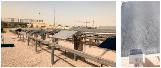
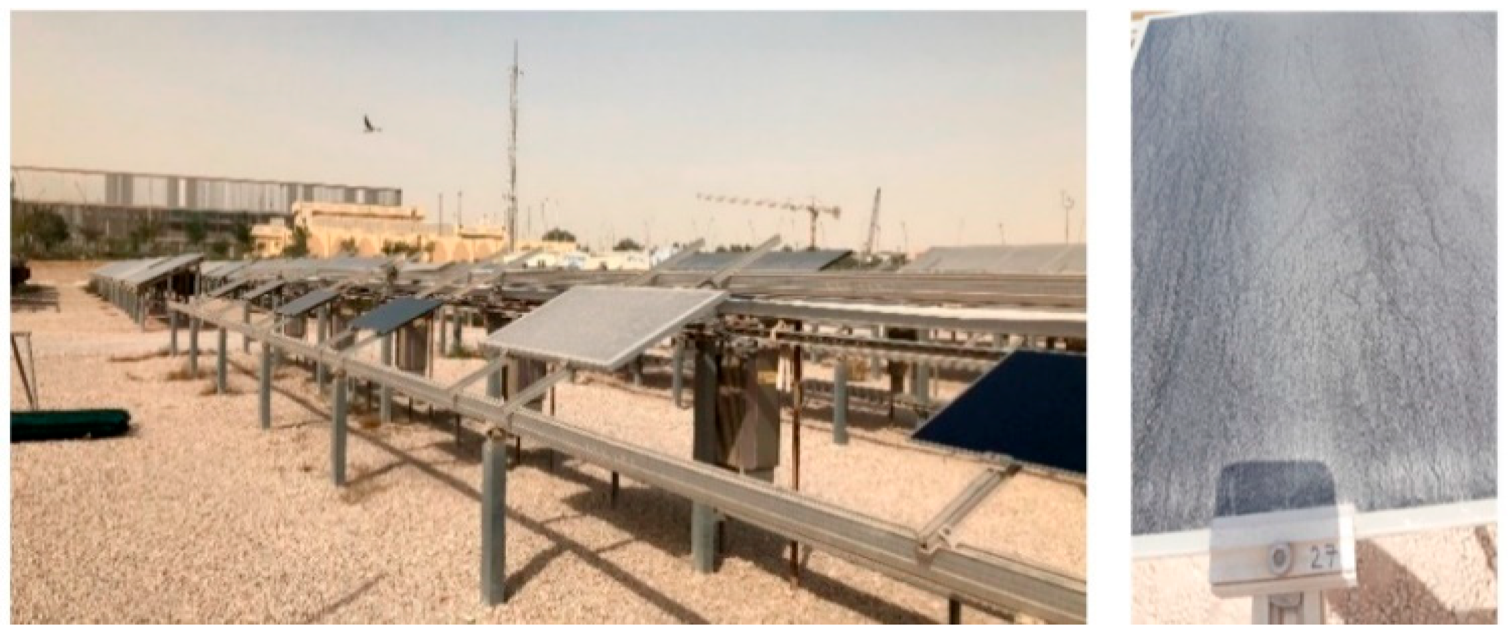
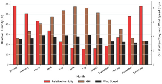
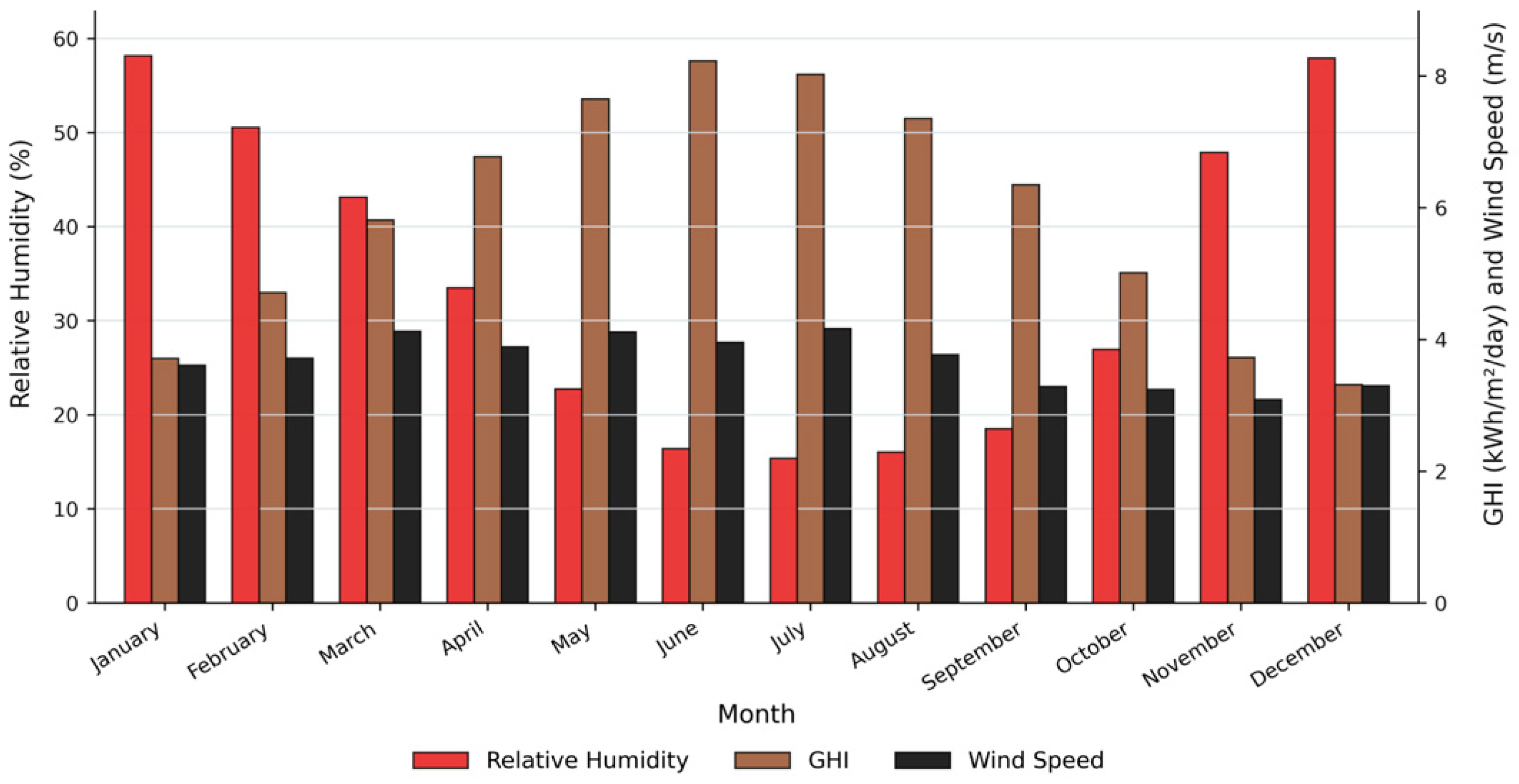
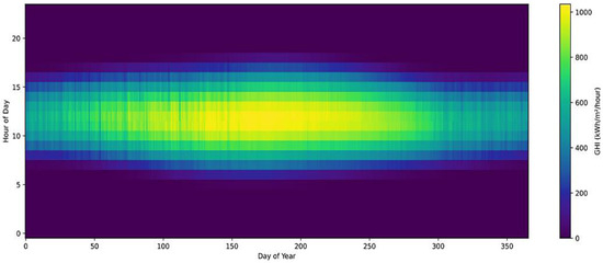
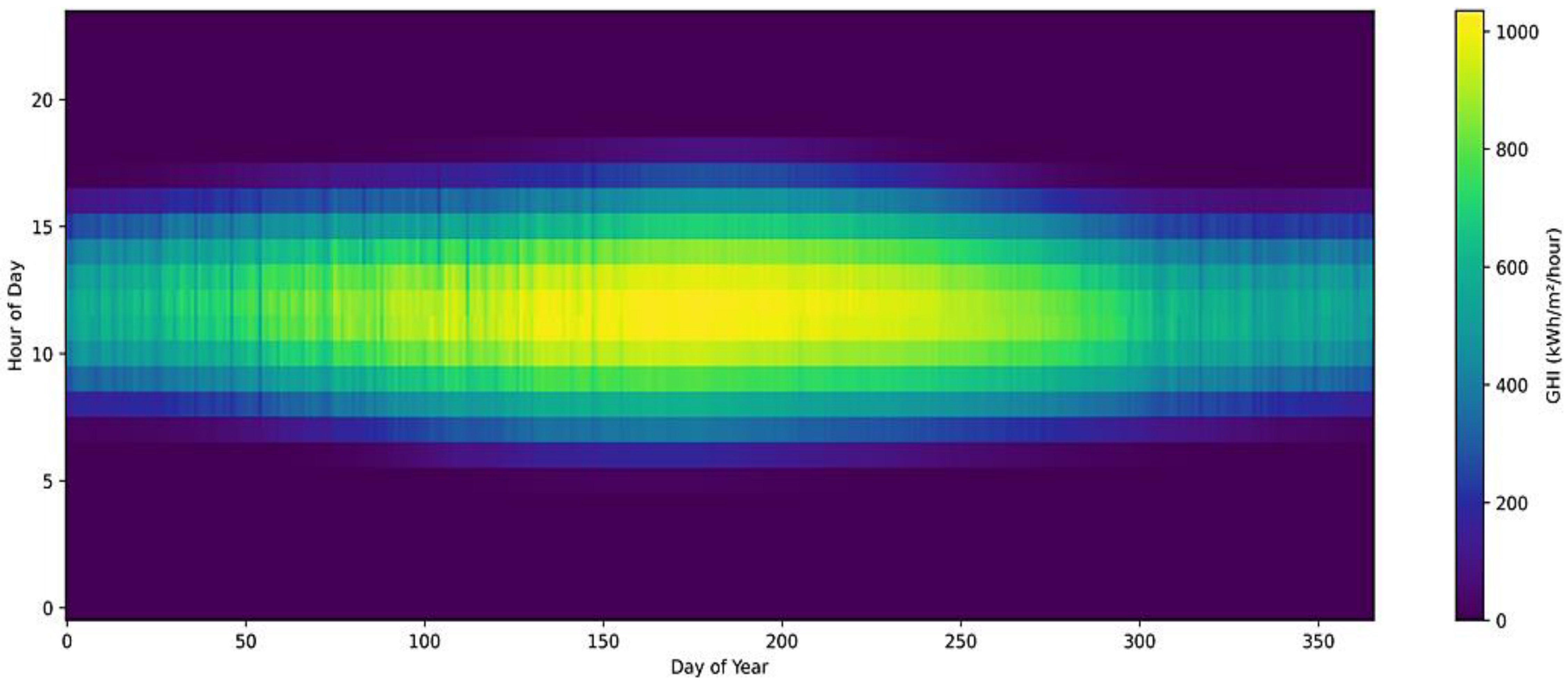
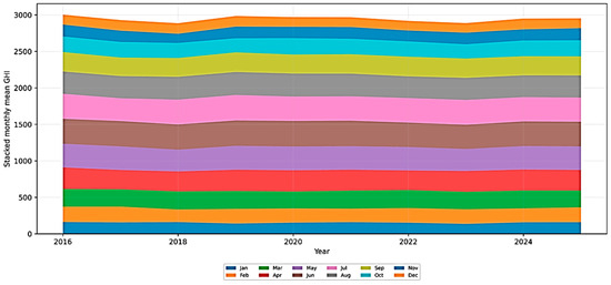
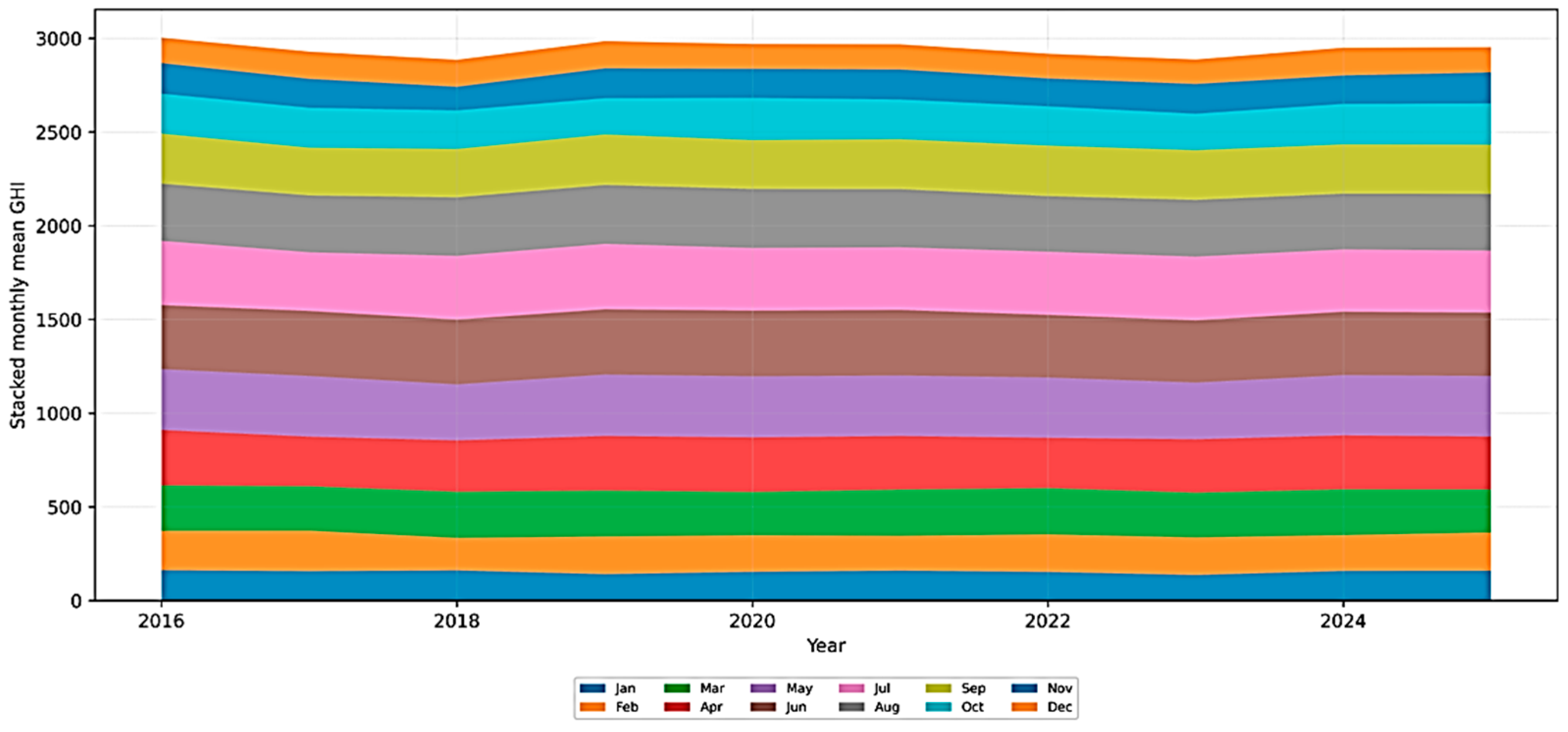
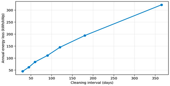
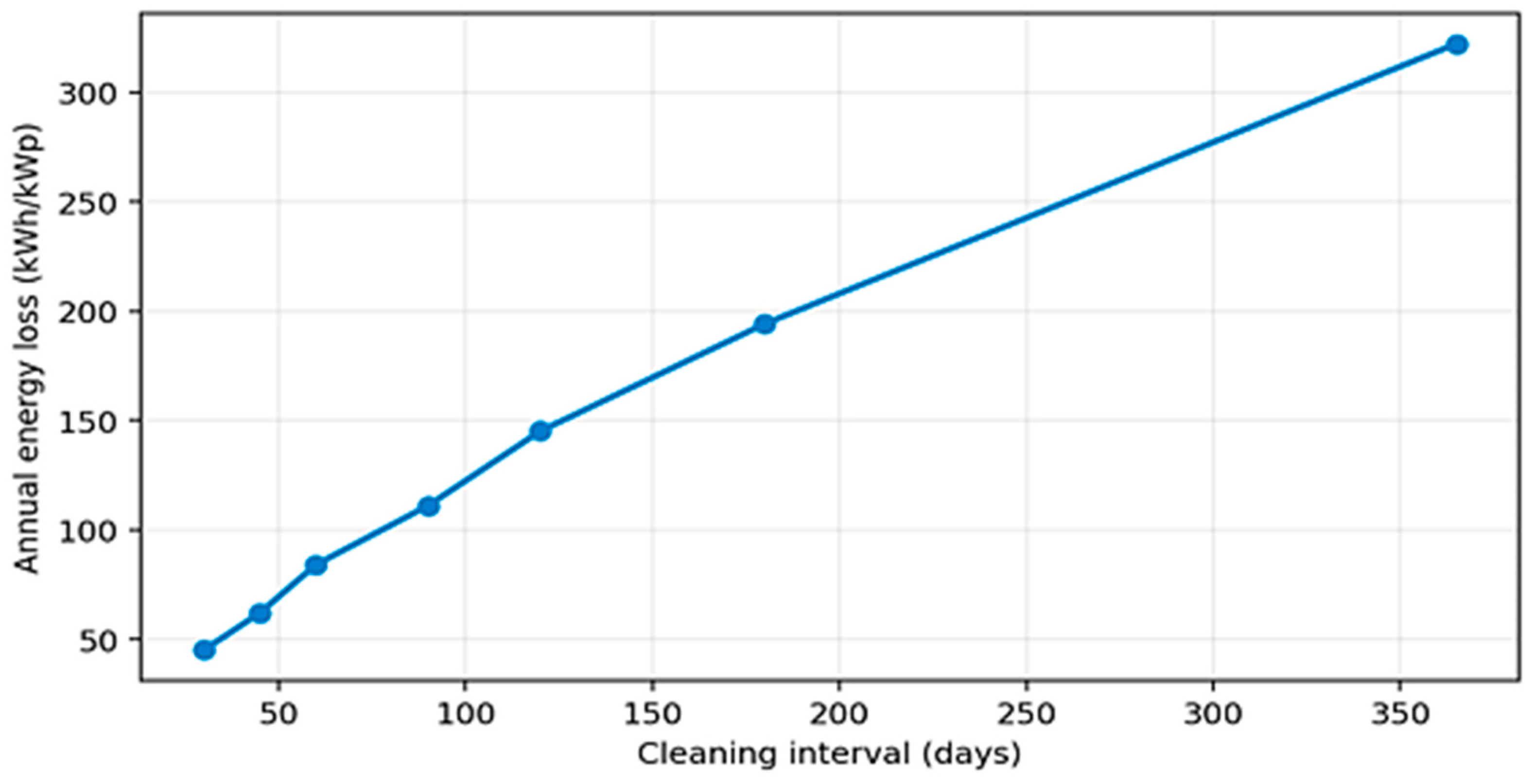
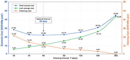
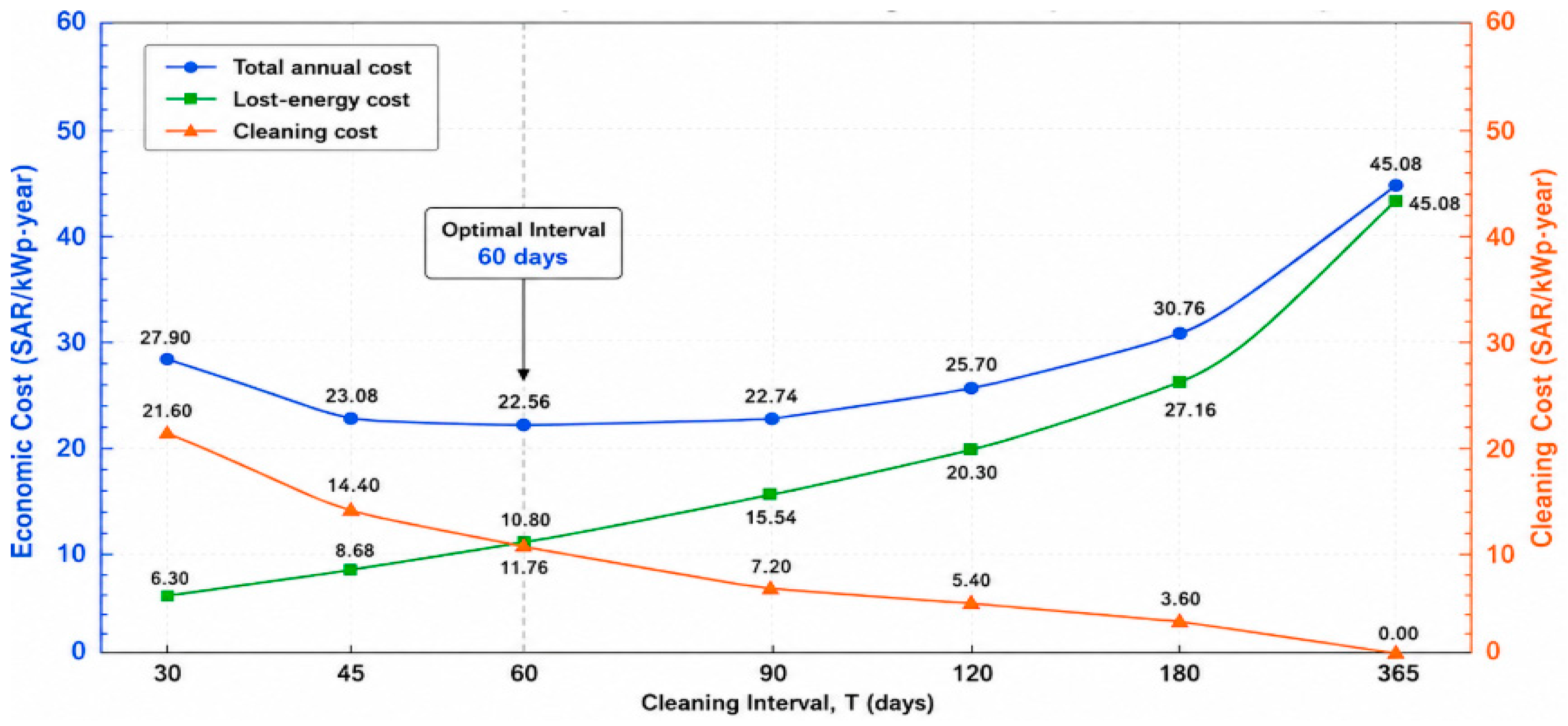
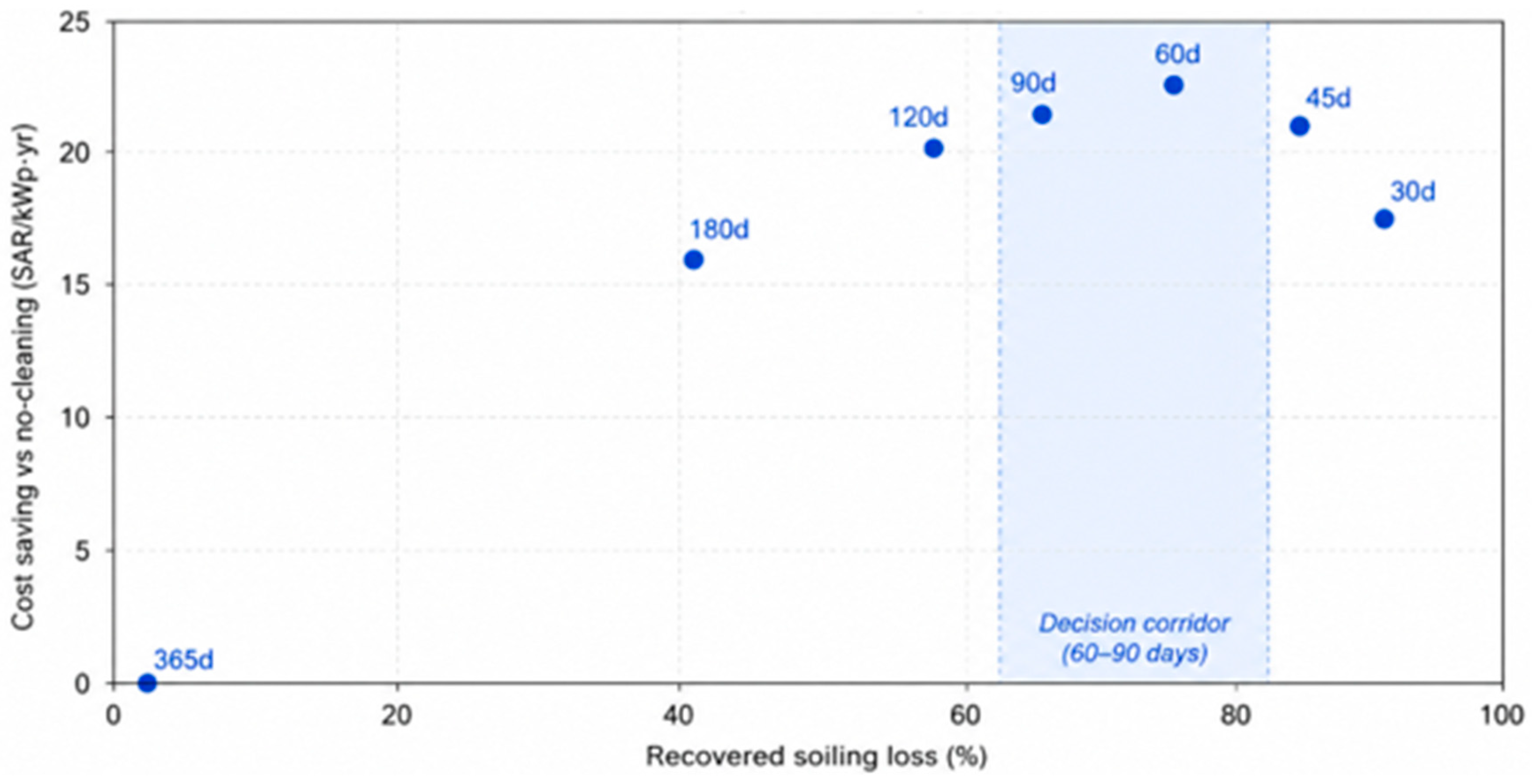
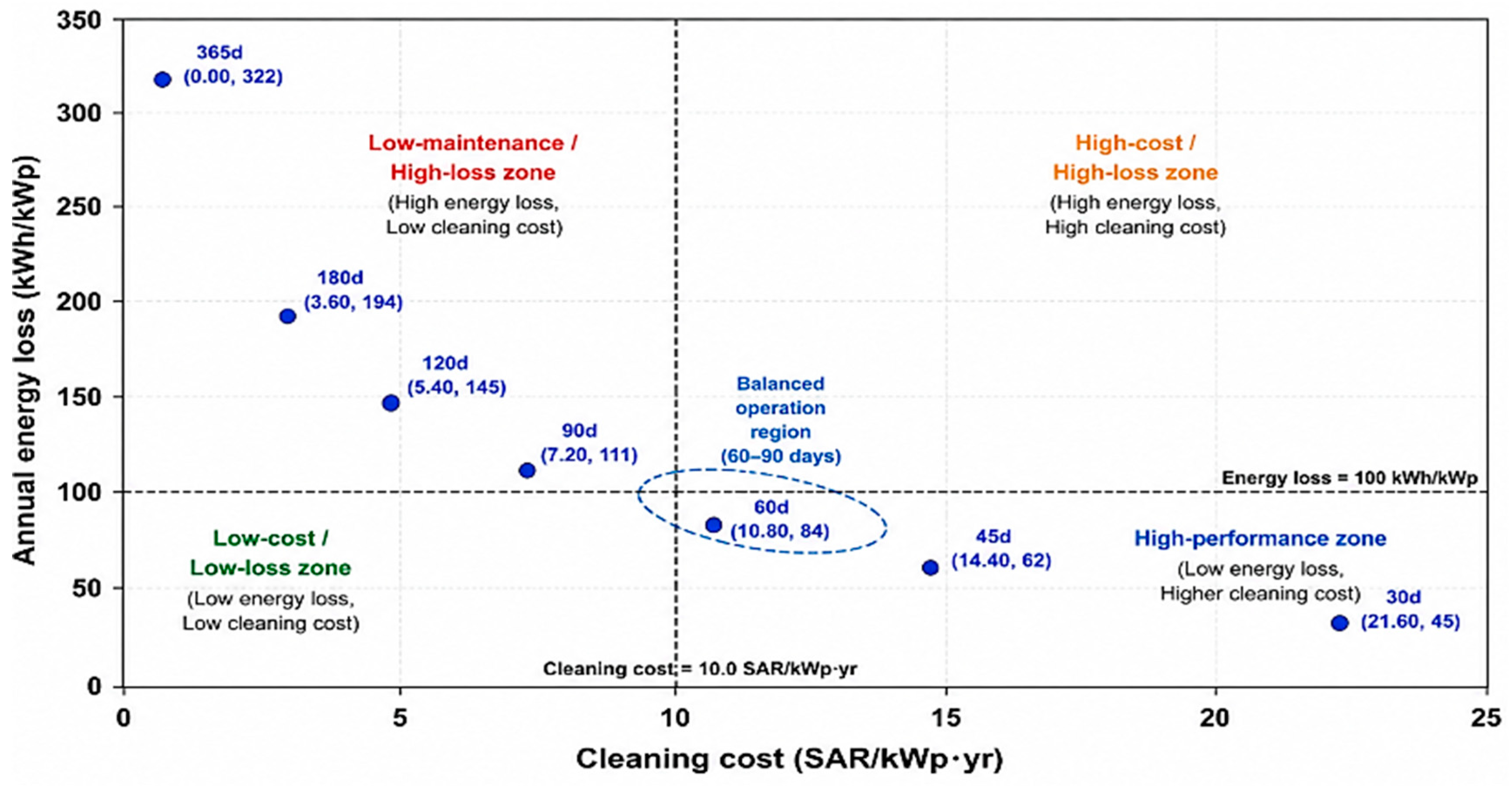
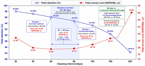
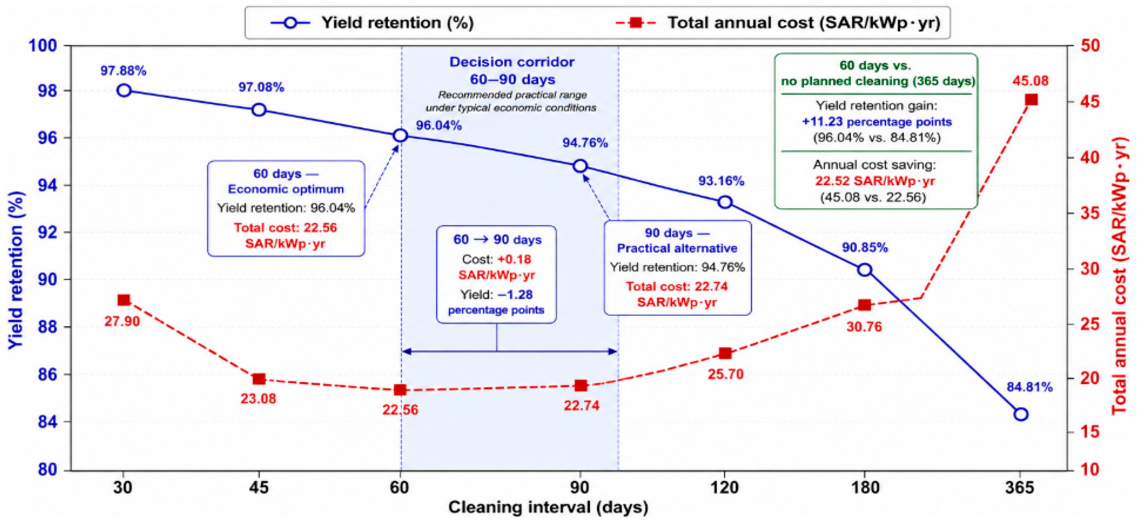

Disclaimer/Publisher’s Note: The statements, opinions and data contained in all publications are solely those of the individual author(s) and contributor(s) and not of MDPI and/or the editor(s). MDPI and/or the editor(s) disclaim responsibility for any injury to people or property resulting from any ideas, methods, instructions or products referred to in the content. |
© 2026 by the author. Licensee MDPI, Basel, Switzerland. This article is an open access article distributed under the terms and conditions of the Creative Commons Attribution (CC BY) license.