Dynamic Scheduling of a Photovoltaic–Storage Office Building with Heating, Ventilation, and Air-Conditioning and Electric-Vehicle Flexibility

Abstract

High photovoltaic (PV) penetration can create hourly mismatches among office-building demand, renewable generation, electricity prices, and grid carbon intensity. This study develops a reproducible, deterministic, time-coupled day-ahead mixed-integer linear programming model for a predetermined PV–battery energy storage system (BESS), simplified heating, ventilation, and air-conditioning (HVAC) load response, and electric-vehicle (EV) charging/vehicle-to-building operation. Separate charging and discharging variables, binary operating states, a cyclic 50% BESS terminal state of charge, and PV- and grid-origin battery accounts eliminate simultaneous operation, initial-energy depletion, and grid-to-BESS-to-grid arbitrage. Five scenarios and five one-factor-at-a-time sensitivity families are independently re-optimized for a Suzhou office-building case. For the selected summer day, Scenario 2 costs 1974.04 CNY. Scenario 3 costs 1974.73 CNY before DR revenue, earns 323.85 CNY, and has a net cost of 1650.88 CNY. Its grid import and grid-side emissions are 1.27% and 1.28% below Scenario 2, respectively, whereas its pre-incentive cost is 0.04% higher. The corrected DR formulation leaves the reported optima unchanged within 2.6 × 10⁻⁹. The maximum hourly balance residual across all runs is 1.3 × 10⁻⁹ kW.

1. Introduction

Buildings with rooftop or project-scale PV increasingly face a temporal-matching problem: solar production, end-use demand, retail tariffs, grid carbon intensity, and flexible device states change at different hours. PV–BESS scheduling can shift grid exchange and reduce short-term electricity charges, but the result depends on battery boundary conditions, conversion losses, and market rules [1,2,3,4,5,6]. HVAC thermal flexibility and EV/V2B can add demand-side response, although their physical and behavioral limits must be represented transparently [7,8,9,10,11,12,13].

Recent building-energy studies have coordinated PV and storage under time-of-use (TOU) prices, while other work has examined HVAC response, EV charging, or carbon-aware operation separately [14,15,16,17,18,19,20,21]. These studies show that storage can move electricity exchange away from high-price periods, HVAC can provide short-duration electrical response, and connected EVs can shift charging or discharge to the building. Related thermal studies, including the heat-extraction analysis of coaxial deep-borehole heat exchangers, further demonstrate why simplified building-response models should not be interpreted as high-fidelity thermal validation [22,23,24]. However, several gaps remain: integrated studies do not always impose cyclic terminal battery conditions; signed storage power can hide simultaneous charging and discharging; total export may not identify the origin of stored energy; and policy incentive revenue is sometimes conflated with technical operating benefit.

Dynamic carbon signals create an additional scheduling dimension. Hourly provincial electricity carbon-emission factors can differ materially within a day, so a constant annual factor cannot represent the timing effect of grid imports [25,26,27,28]. At the same time, the economic value of demand response is policy-dependent and must be separated from electricity-cost and carbon-cost components [29,30,31]. A credible computational case therefore requires complete hourly inputs, explicit baseline and response definitions, origin-resolved energy flows, reported cost coefficients, solver settings, and auditable raw results.

The contributions of this study are:

• A physically closed MILP coordination framework for PV, BESS, simplified HVAC electrical response, and EV/V2B, using 24 power intervals and 25 energy-state nodes;
• Binary mutual-exclusion constraints for BESS charging/discharging, EV charging/V2B, and grid import/export, together with a cyclic 50% BESS terminal state;
• Two virtual BESS energy accounts that distinguish PV-origin and grid-origin electricity and prohibit grid-origin battery export;
• Joint economic and carbon-aware scheduling with transparent separation of operating cost before incentives, demand-response revenue, net operating cost, and a separate BESS CAPEX screening calculation;
• Five base scenarios, including HVAC-only and EV-only ablations, plus independently re-optimized sensitivities for BESS capacity, EV penetration, DR incentive, TOU spread, and carbon price, each compared with a matched Scenario 2 baseline.

2. Materials and Methods

2.1. Problem Definition and Nomenclature

The optimization minimizes one-day net operating cost subject to hourly energy-flow, device-state, and boundary constraints. Prices, PV availability, building loads, EV connection flags, DR intervals, and hourly carbon factors are exogenous parameters. Charging and discharging powers are split into nonnegative variables, and logical states are binary. All remaining expressions are linear; no product between continuous decision variables is retained. The resulting formulation is a MILP. Table 1 is the nomenclature used in the revised MILP formulation.

Table 1. Nomenclature used in the revised MILP formulation.

Symbol	Definition	Unit
$\mathrm{t}$	Hourly power interval, t = 0, …, 23	–
$\mathrm{n}$	Energy-state node, n = 0, …, 24	–
$\mathrm{i}$	EV index	–
$\mathcal{T}$	Set of 24 hourly intervals	–
$\mathcal{N}$	Set of 25 state nodes	–
${\mathrm{N}}_{\mathrm{y}}$	Economic lifetime used in the capital-recovery factor	year
$\mathcal{I}$	Set of connected EVs	–
${\mathrm{P}}_{\mathrm{g}\mathrm{r}\mathrm{i}\mathrm{d},\mathrm{t}}^{\mathrm{b}\mathrm{u}\mathrm{y}}/{\mathrm{P}}_{\mathrm{g}\mathrm{r}\mathrm{i}\mathrm{d},\mathrm{t}}^{\mathrm{s}\mathrm{e}\mathrm{l}\mathrm{l}}$	Grid import/export power	kW
${\mathrm{P}}_{\mathrm{P}\mathrm{V}\to \mathrm{l}\mathrm{o}\mathrm{a}\mathrm{d},\mathrm{t}}$	PV power supplied directly to load	kW
${\mathrm{P}}_{\mathrm{P}\mathrm{V}\to \mathrm{B}\mathrm{E}\mathrm{S}\mathrm{S},\mathrm{t}}$	PV power charged to BESS	kW
${\mathrm{P}}_{\mathrm{P}\mathrm{V},\mathrm{s}\mathrm{e}\mathrm{l}\mathrm{l},\mathrm{t}}/{\mathrm{P}}_{\mathrm{P}\mathrm{V},\mathrm{c}\mathrm{u}\mathrm{r}\mathrm{t},\mathrm{t}}$	Direct PV export/curtailment	kW
${\mathrm{P}}_{\mathrm{g}\mathrm{r}\mathrm{i}\mathrm{d}\to \mathrm{l}\mathrm{o}\mathrm{a}\mathrm{d},\mathrm{t}}/{\mathrm{P}}_{\mathrm{g}\mathrm{r}\mathrm{i}\mathrm{d}\to \mathrm{B}\mathrm{E}\mathrm{S}\mathrm{S},\mathrm{t}}$	Grid power supplied to load/BESS	kW
${\mathrm{P}}_{\mathrm{B}\mathrm{E}\mathrm{S}\mathrm{S},\mathrm{t}}^{\mathrm{c}\mathrm{h}}/{\mathrm{P}}_{\mathrm{B}\mathrm{E}\mathrm{S}\mathrm{S},\mathrm{t}}^{\mathrm{d}\mathrm{i}\mathrm{s}}$	BESS charging/discharging power	kW
${\mathrm{P}}_{\mathrm{B}\mathrm{E}\mathrm{S}\mathrm{S},\mathrm{P}\mathrm{V}\to \mathrm{l}\mathrm{o}\mathrm{a}\mathrm{d},\mathrm{t}}$	PV-origin BESS discharge to load	kW
${\mathrm{P}}_{\mathrm{B}\mathrm{E}\mathrm{S}\mathrm{S},\mathrm{P}\mathrm{V}\to \mathrm{g}\mathrm{r}\mathrm{i}\mathrm{d},\mathrm{t}}$	PV-origin BESS discharge to grid	kW
${\mathrm{P}}_{\mathrm{B}\mathrm{E}\mathrm{S}\mathrm{S},\mathrm{g}\mathrm{r}\mathrm{i}\mathrm{d}\to \mathrm{l}\mathrm{o}\mathrm{a}\mathrm{d},\mathrm{t}}$	Grid-origin BESS discharge to load	kW
${\mathrm{E}}_{\mathrm{B}\mathrm{E}\mathrm{S}\mathrm{S},\mathrm{n}}$	Total BESS stored energy	kWh
${\mathrm{E}}_{\mathrm{B}\mathrm{E}\mathrm{S}\mathrm{S},\mathrm{n}}^{\mathrm{P}\mathrm{V}}/{\mathrm{E}}_{\mathrm{B}\mathrm{E}\mathrm{S}\mathrm{S},\mathrm{n}}^{\mathrm{g}\mathrm{r}\mathrm{i}\mathrm{d}}$	PV-origin/grid-origin BESS energy account	kWh
${\mathrm{S}\mathrm{O}\mathrm{C}}_{\mathrm{B}\mathrm{E}\mathrm{S}\mathrm{S},\mathrm{n}}$	BESS state of charge	p.u.
${\mathrm{P}}_{\mathrm{E}\mathrm{V},\mathrm{i},\mathrm{t}}^{\mathrm{c}\mathrm{h}}/{\mathrm{P}}_{\mathrm{E}\mathrm{V},\mathrm{i},\mathrm{t}}^{\mathrm{d}\mathrm{i}\mathrm{s}}$	EV charging/V2B power	kW
${\mathrm{E}}_{\mathrm{E}\mathrm{V},\mathrm{i},\mathrm{n}}/{\mathrm{S}\mathrm{O}\mathrm{C}}_{\mathrm{E}\mathrm{V},\mathrm{i},\mathrm{n}}$	EV stored energy/state of charge	kWh/p.u.
${\mathrm{P}}_{\mathrm{H}\mathrm{V}\mathrm{A}\mathrm{C},\mathrm{t}}$	Scheduled HVAC electrical power	kW
$\mathsf{\Delta }{\mathrm{P}}_{\mathrm{H}\mathrm{V}\mathrm{A}\mathrm{C},\mathrm{t}}^{\mathrm{d}\mathrm{o}\mathrm{w}\mathrm{n}}/\mathsf{\Delta }{\mathrm{P}}_{\mathrm{H}\mathrm{V}\mathrm{A}\mathrm{C},\mathrm{t}}^{\mathrm{u}\mathrm{p}}$	HVAC load reduction/recovery	kW
${\mathrm{P}}_{\mathrm{D}\mathrm{R},\mathrm{t}}$	Verified incentivized DR response power	kW
${\mathrm{u}}_{\mathrm{B}\mathrm{E}\mathrm{S}\mathrm{S},\mathrm{t}}^{\mathrm{c}\mathrm{h}}/{\mathrm{u}}_{\mathrm{B}\mathrm{E}\mathrm{S}\mathrm{S},\mathrm{t}}^{\mathrm{d}\mathrm{i}\mathrm{s}}$	BESS charging/discharging state	0 or 1
${\mathrm{u}}_{\mathrm{E}\mathrm{V},\mathrm{i},\mathrm{t}}^{\mathrm{c}\mathrm{h}}/{\mathrm{u}}_{\mathrm{E}\mathrm{V},\mathrm{i},\mathrm{t}}^{\mathrm{d}\mathrm{i}\mathrm{s}}$	EV charging/V2B state	0 or 1
${\mathrm{u}}_{\mathrm{g}\mathrm{r}\mathrm{i}\mathrm{d},\mathrm{t}}^{\mathrm{b}\mathrm{u}\mathrm{y}}/{\mathrm{u}}_{\mathrm{g}\mathrm{r}\mathrm{i}\mathrm{d},\mathrm{t}}^{\mathrm{s}\mathrm{e}\mathrm{l}\mathrm{l}}$	Grid import/export state	0 or 1
${\mathrm{P}}_{\mathrm{r}\mathrm{i}\mathrm{g}\mathrm{i}\mathrm{d},\mathrm{t}}/{\mathrm{P}}_{\mathrm{H}\mathrm{V}\mathrm{A}\mathrm{C},\mathrm{t}}^{\mathrm{b}\mathrm{a}\mathrm{s}\mathrm{e}}$	Rigid/baseline HVAC electrical load	kW
${\mathrm{P}}_{\mathrm{P}\mathrm{V},\mathrm{t}}^{\mathrm{a}\mathrm{v}\mathrm{a}\mathrm{i}\mathrm{l}}$	Available PV power	kW
${\mathrm{a}}_{\mathrm{i},\mathrm{t}}$	EV connection status	0 or 1
${\mathsf{\lambda }}_{\mathrm{t}}^{\mathrm{b}\mathrm{u}\mathrm{y}}/{\mathsf{\lambda }}_{\mathrm{t}}^{\mathrm{s}\mathrm{e}\mathrm{l}\mathrm{l}}$	Electricity purchase/selling price	CNY/kWh
${\mathsf{\gamma }}_{\mathrm{t}}$	Hourly grid carbon-emission factor	kgCO2/kWh
${\mathsf{\pi }}_{\mathrm{C}\mathrm{O}2}$	Carbon price	CNY/kgCO2
${\mathrm{k}}_{\mathrm{D}\mathrm{R}}$	DR incentive coefficient	CNY/kWh
${\mathrm{b}}_{\mathrm{D}\mathrm{R},\mathrm{t}}$	Declared DR interval flag	0 or 1
${\mathrm{P}}_{\mathrm{g}\mathrm{r}\mathrm{i}\mathrm{d},\mathrm{t}}^{\mathrm{b}\mathrm{a}\mathrm{s}\mathrm{e}}$	S2 baseline grid-import power	kW
${\mathsf{\eta }}_{\mathrm{B}\mathrm{E}\mathrm{S}\mathrm{S}}^{\mathrm{c}\mathrm{h}}/{\mathsf{\eta }}_{\mathrm{B}\mathrm{E}\mathrm{S}\mathrm{S}}^{\mathrm{d}\mathrm{i}\mathrm{s}}$	BESS charge/discharge efficiency	p.u.
${\mathsf{\eta }}_{\mathrm{E}\mathrm{V}}^{\mathrm{c}\mathrm{h}}/{\mathsf{\eta }}_{\mathrm{E}\mathrm{V}}^{\mathrm{d}\mathrm{i}\mathrm{s}}$	EV charge/discharge efficiency	p.u.
${\mathrm{c}}_{\mathrm{P}\mathrm{V}}/{\mathrm{c}}_{\mathrm{B}\mathrm{E}\mathrm{S}\mathrm{S}}/{\mathrm{c}}_{\mathrm{H}\mathrm{V}\mathrm{A}\mathrm{C}}/{\mathrm{c}}_{\mathrm{E}\mathrm{V}}$	PV O&M, BESS throughput, HVAC response, EV V2B costs	CNY/kWh
${\mathrm{P}}_{\mathrm{E}\mathrm{V},\mathrm{t}}^{\mathrm{f}\mathrm{i}\mathrm{x}\mathrm{e}\mathrm{d}}$	Fixed EV charging baseline used for DR verification	kW
${\mathrm{E}}_{\mathrm{P}\mathrm{V},\mathrm{u}\mathrm{s}\mathrm{e}\mathrm{d}}$	PV energy used directly, charged to BESS, or exported	kWh
${\mathrm{E}}_{\mathrm{B}\mathrm{E}\mathrm{S}\mathrm{S},\mathrm{t}\mathrm{h}\mathrm{r}\mathrm{o}\mathrm{u}\mathrm{g}\mathrm{h}}$	BESS charge-plus-discharge throughput energy	kWh
${\mathrm{E}}_{\mathrm{H}\mathrm{V}\mathrm{A}\mathrm{C},\mathrm{d}\mathrm{o}\mathrm{w}\mathrm{n}}$	Cumulative scheduled HVAC load-reduction energy	kWh
${\mathrm{E}}_{\mathrm{E}\mathrm{V},\mathrm{V}2\mathrm{B}}$	Cumulative EV discharge energy supplied through V2B	kWh
$\mathrm{B}\mathrm{E}\mathrm{S}\mathrm{S}$	Battery energy storage system	–
$\mathrm{D}\mathrm{R}/\mathrm{E}\mathrm{V}/\mathrm{H}\mathrm{V}\mathrm{A}\mathrm{C}/\mathrm{M}\mathrm{I}\mathrm{L}\mathrm{P}/\mathrm{P}\mathrm{V}/\mathrm{S}\mathrm{O}\mathrm{C}/\mathrm{T}\mathrm{O}\mathrm{U}/\mathrm{V}2\mathrm{B}$	Demand response/electric vehicle/heating, ventilation, and air-conditioning/mixed-integer linear programming/photovoltaic/state of charge/time of use/vehicle to building	–
${\mathrm{d}}_{\mathrm{g}\mathrm{r}\mathrm{i}\mathrm{d},\mathrm{t}}/{\mathrm{d}}_{\mathrm{f}\mathrm{l}\mathrm{e}\mathrm{x},\mathrm{t}}$	Grid-import and flexible-resource differences used for DR verification	kW
${\mathrm{P}}_{\mathrm{g}\mathrm{r}\mathrm{i}\mathrm{d},\mathrm{t}}^{+}/{\mathrm{P}}_{\mathrm{f}\mathrm{l}\mathrm{e}\mathrm{x},\mathrm{t}}^{+}$	Exact positive parts of the grid and flexible-resource differences	kW
${\mathrm{z}}_{\mathrm{g}\mathrm{r}\mathrm{i}\mathrm{d},\mathrm{t}}/{\mathrm{z}}_{\mathrm{f}\mathrm{l}\mathrm{e}\mathrm{x},\mathrm{t}}$	Binary sign indicators for the two positive-part relations	0 or 1
${\mathrm{M}}_{\mathrm{g}\mathrm{r}\mathrm{i}\mathrm{d}}/{\mathrm{M}}_{\mathrm{f}\mathrm{l}\mathrm{e}\mathrm{x}}$	Valid Big-M bounds for the grid and flexible-resource differences	kW

2.2. Case Study and Hourly Inputs

2.2.1. Office Building, PV System, BESS, and EV Fleet

The case represents an office-building project in Suzhou, Jiangsu Province, China. The confirmed electrical PV design comprises 840 modules rated at 450 Wp each, giving 378 kWp installed capacity. The module dimensions are approximately 2108 mm × 1048 mm, corresponding to an aggregate module surface of approximately 1855.7 m². The dispatch model uses the 378 kWp installed capacity and hourly PV availability.

The predetermined base-case BESS is 1000 kWh with a 0.5 C power rating (500 kW maximum charging or discharging power). The base fleet contains 10 EVs, each with 57 kWh capacity and 11.4 kW bidirectional charger limits. Vehicles arrive at state node 8 with 30% SOC, remain connected through the working-day window, and must reach at least 80% SOC at departure node 18.

2.2.2. Tariff, Carbon Factor, and Demand-Response Inputs

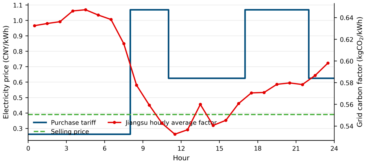
The archived project settlement tariff is 0.2627 CNY/kWh at 00:00–08:00, 1.0694 CNY/kWh at 08:00–11:00 and 17:00–22:00, and 0.6254 CNY/kWh at 11:00–17:00 and 22:00–24:00. The selling price is 0.391 CNY/kWh under the archived Jiangsu benchmark-price assumption.

The hourly carbon series is the Jiangsu 2025 baseline-scenario profile for 25 July extracted from dataset hours 4921–4944 of Li et al. [32]. It is a projected hourly average consumption-based provincial electricity carbon-emission factor. The values range from 0.5325 to 0.6473 kgCO₂/kWh. A base carbon price of 80 CNY/tCO₂ (0.08 CNY/kgCO₂) converts grid-import emissions into an objective-function cost.

The declared DR intervals are 08:00–11:00 and 17:00–19:00. The base coefficient is 3 CNY/kWh, consistent with the ceiling for day-ahead peak-shaving energy subsidies in the 2024 Jiangsu demand-response implementation rules [33]. Actual payments are market- and bidding-dependent. The baseline is the independently optimized Scenario 2 grid-import profile under otherwise identical inputs. A response is credited only when it is both a nonnegative reduction from that baseline and physically attributable to HVAC or EV/V2B response. Table 2 summarizes the principal model inputs and their provenance, and data sources, tariffs, carbon factors, and the 24-h load and PV curves are included in Supplementary File S1.

Table 2. Principal input data and provenance.

Input	Source and Treatment	Unit
Rigid and HVAC loads; PV availability; EV baseline	Archived case-study figures; reconstructed hourly series	kW
Purchase tariff	Archived project settlement input; Jiangsu TOU period framework	CNY/kWh
Selling price	Archived Jiangsu benchmark on-grid price [34]	CNY/kWh
Grid carbon factor	Li et al. 2026 dataset, Jiangsu, 25 July 2025, baseline scenario [32]	kgCO2/kWh
DR intervals and ceiling	Jiangsu 2024 implementation rules [33]	h; CNY/kWh
BESS screening benchmark	NREL 2024 ATB commercial battery storage [35]	USD/kWh; USD/kW

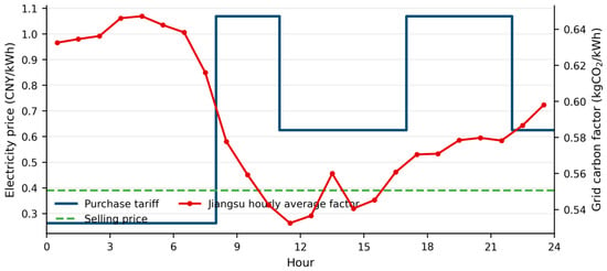
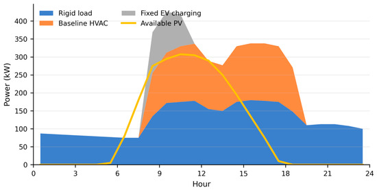
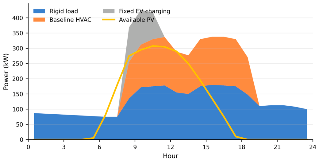
Figure 1 shows a stepped time-of-use purchase tariff and a constant selling price, while the projected grid carbon factor decreases from an early-morning maximum to a midday minimum and subsequently rises toward the evening. Thus, the electricity-price and carbon signals are not perfectly aligned over the day. Figure 2 shows that PV generation is concentrated in daylight hours and broadly overlaps the daytime office load, whereas fixed EV charging adds a pronounced morning demand block and little PV power is available during the late-afternoon and evening load period.

Figure 1. Hourly purchase tariff, selling price, and projected Jiangsu average consumption-based grid carbon-emission factor.

Figure 2. Reconstructed rigid load, baseline HVAC load, fixed EV charging demand, and available PV power for the selected typical summer day.

2.2.3. Scenario and Sensitivity Design

One-factor-at-a-time sensitivities re-optimize the full S3 model for BESS capacities of 500, 1000, and 1500 kWh (each at 0.5 C); EV fleets of 10, 20, and 30 vehicles; DR coefficients of 0, 1.5, and 3 CNY/kWh; TOU peak-to-valley spreads of 80%, 100%, and 120% while retaining the base-case daily average purchase price; and carbon prices of 40, 80, and 120 CNY/tCO₂. For every level, a matching S2 baseline is also independently solved before S3 response is credited. Table 3 defines five scenarios that isolate the contributions of BESS, HVAC response, and flexible EV/V2B operation, with S3 representing the fully coordinated configuration and S4–S5 serving as ablation cases.

Table 3. Base-scenario definitions.

Scenario	Configuration	BESS	HVAC Response	EV Operation
S1	PV only	No	No	Fixed
S2	PV + BESS	Yes	No	Fixed
S3	PV + BESS + HVAC + EV/V2B	Yes	Yes	Flexible
S4	PV + BESS + HVAC	Yes	Yes	Fixed
S5	PV + BESS + EV/V2B	Yes	No	Flexible

2.3. Integrated MILP Formulation

2.3.1. Flow Decomposition and Hourly Power Balance

Available PV is assigned exactly once to direct load supply, BESS charging, direct export, or curtailment:

$${\mathrm{P}}_{\mathrm{P}\mathrm{V}\to \mathrm{l}\mathrm{o}\mathrm{a}\mathrm{d},\mathrm{t}}+{\mathrm{P}}_{\mathrm{P}\mathrm{V}\to \mathrm{B}\mathrm{E}\mathrm{S}\mathrm{S},\mathrm{t}}+{\mathrm{P}}_{\mathrm{P}\mathrm{V},\mathrm{s}\mathrm{e}\mathrm{l}\mathrm{l},\mathrm{t}}+{\mathrm{P}}_{\mathrm{P}\mathrm{V},\mathrm{c}\mathrm{u}\mathrm{r}\mathrm{t},\mathrm{t}}={\mathrm{P}}_{\mathrm{P}\mathrm{V},\mathrm{t}}^{\mathrm{a}\mathrm{v}\mathrm{a}\mathrm{i}\mathrm{l}}.$$

(1)

Grid import is divided between direct load supply and BESS charging, while export contains only direct PV export and PV-origin BESS discharge:

$${\mathrm{P}}_{\mathrm{g}\mathrm{r}\mathrm{i}\mathrm{d},\mathrm{t}}^{\mathrm{b}\mathrm{u}\mathrm{y}}={\mathrm{P}}_{\mathrm{g}\mathrm{r}\mathrm{i}\mathrm{d}\to \mathrm{l}\mathrm{o}\mathrm{a}\mathrm{d},\mathrm{t}}+{\mathrm{P}}_{\mathrm{g}\mathrm{r}\mathrm{i}\mathrm{d}\to \mathrm{B}\mathrm{E}\mathrm{S}\mathrm{S},\mathrm{t}},$$

(2)

$${\mathrm{P}}_{\mathrm{g}\mathrm{r}\mathrm{i}\mathrm{d},\mathrm{t}}^{\mathrm{s}\mathrm{e}\mathrm{l}\mathrm{l}}={\mathrm{P}}_{\mathrm{P}\mathrm{V},\mathrm{s}\mathrm{e}\mathrm{l}\mathrm{l},\mathrm{t}}+{\mathrm{P}}_{\mathrm{B}\mathrm{E}\mathrm{S}\mathrm{S},\mathrm{P}\mathrm{V}\to \mathrm{g}\mathrm{r}\mathrm{i}\mathrm{d},\mathrm{t}}.$$

(3)

The building-side hourly balance excludes charging and export because those flows are already represented by their upstream splits:

$$\begin{array}{c}{\mathrm{P}}_{\mathrm{P}\mathrm{V}\to \mathrm{l}\mathrm{o}\mathrm{a}\mathrm{d},\mathrm{t}}+{\mathrm{P}}_{\mathrm{g}\mathrm{r}\mathrm{i}\mathrm{d}\to \mathrm{l}\mathrm{o}\mathrm{a}\mathrm{d},\mathrm{t}}+{\mathrm{P}}_{\mathrm{B}\mathrm{E}\mathrm{S}\mathrm{S},\mathrm{P}\mathrm{V}\to \mathrm{l}\mathrm{o}\mathrm{a}\mathrm{d},\mathrm{t}}+{\mathrm{P}}_{\mathrm{B}\mathrm{E}\mathrm{S}\mathrm{S},\mathrm{g}\mathrm{r}\mathrm{i}\mathrm{d}\to \mathrm{l}\mathrm{o}\mathrm{a}\mathrm{d},\mathrm{t}}\\ +\sum _{\mathrm{i}\in \mathcal{I}}{\mathrm{P}}_{\mathrm{E}\mathrm{V},\mathrm{i},\mathrm{t}}^{\mathrm{d}\mathrm{i}\mathrm{s}}={\mathrm{P}}_{\mathrm{r}\mathrm{i}\mathrm{g}\mathrm{i}\mathrm{d},\mathrm{t}}+{\mathrm{P}}_{\mathrm{H}\mathrm{V}\mathrm{A}\mathrm{C},\mathrm{t}}+\sum _{\mathrm{i}\in \mathcal{I}}{\mathrm{P}}_{\mathrm{E}\mathrm{V},\mathrm{i},\mathrm{t}}^{\mathrm{c}\mathrm{h}}\end{array}.$$

(4)

2.3.2. BESS Variables, Mutual Exclusion, Cyclic State, and Energy Origin

Signed BESS power is reported for visualization, but the optimization uses separate nonnegative charging and discharging variables:

$${\mathrm{P}}_{\mathrm{B}\mathrm{E}\mathrm{S}\mathrm{S},\mathrm{t}}^{\mathrm{n}\mathrm{e}\mathrm{t}}={\mathrm{P}}_{\mathrm{B}\mathrm{E}\mathrm{S}\mathrm{S},\mathrm{t}}^{\mathrm{d}\mathrm{i}\mathrm{s}}-{\mathrm{P}}_{\mathrm{B}\mathrm{E}\mathrm{S}\mathrm{S},\mathrm{t}}^{\mathrm{c}\mathrm{h}}.$$

(5)

$$0\le {\mathrm{P}}_{\mathrm{B}\mathrm{E}\mathrm{S}\mathrm{S},\mathrm{t}}^{\mathrm{c}\mathrm{h}}\le {\mathrm{u}}_{\mathrm{B}\mathrm{E}\mathrm{S}\mathrm{S},\mathrm{t}}^{\mathrm{c}\mathrm{h}}{\mathrm{P}}_{\mathrm{B}\mathrm{E}\mathrm{S}\mathrm{S},\mathrm{m}\mathrm{a}\mathrm{x}}^{\mathrm{c}\mathrm{h}},$$

(6)

$$0\le {\mathrm{P}}_{\mathrm{B}\mathrm{E}\mathrm{S}\mathrm{S},\mathrm{t}}^{\mathrm{d}\mathrm{i}\mathrm{s}}\le {\mathrm{u}}_{\mathrm{B}\mathrm{E}\mathrm{S}\mathrm{S},\mathrm{t}}^{\mathrm{d}\mathrm{i}\mathrm{s}}{\mathrm{P}}_{\mathrm{B}\mathrm{E}\mathrm{S}\mathrm{S},\mathrm{m}\mathrm{a}\mathrm{x}}^{\mathrm{d}\mathrm{i}\mathrm{s}},$$

(7)

$${\mathrm{u}}_{\mathrm{B}\mathrm{E}\mathrm{S}\mathrm{S},\mathrm{t}}^{\mathrm{c}\mathrm{h}}+{\mathrm{u}}_{\mathrm{B}\mathrm{E}\mathrm{S}\mathrm{S},\mathrm{t}}^{\mathrm{d}\mathrm{i}\mathrm{s}}\le 1,{\mathrm{u}}_{\mathrm{B}\mathrm{E}\mathrm{S}\mathrm{S},\mathrm{t}}^{\mathrm{c}\mathrm{h}},{\mathrm{u}}_{\mathrm{B}\mathrm{E}\mathrm{S}\mathrm{S},\mathrm{t}}^{\mathrm{d}\mathrm{i}\mathrm{s}}\in \left\{0,1\right\}.$$

(8)

The total charging and discharging powers are the sums of their origin-resolved flows:

$${\mathrm{P}}_{\mathrm{B}\mathrm{E}\mathrm{S}\mathrm{S},\mathrm{t}}^{\mathrm{c}\mathrm{h}}={\mathrm{P}}_{\mathrm{P}\mathrm{V}\to \mathrm{B}\mathrm{E}\mathrm{S}\mathrm{S},\mathrm{t}}+{\mathrm{P}}_{\mathrm{g}\mathrm{r}\mathrm{i}\mathrm{d}\to \mathrm{B}\mathrm{E}\mathrm{S}\mathrm{S},\mathrm{t}},$$

(9)

$${\mathrm{P}}_{\mathrm{B}\mathrm{E}\mathrm{S}\mathrm{S},\mathrm{t}}^{\mathrm{d}\mathrm{i}\mathrm{s}}={\mathrm{P}}_{\mathrm{B}\mathrm{E}\mathrm{S}\mathrm{S},\mathrm{P}\mathrm{V}\to \mathrm{l}\mathrm{o}\mathrm{a}\mathrm{d},\mathrm{t}}+{\mathrm{P}}_{\mathrm{B}\mathrm{E}\mathrm{S}\mathrm{S},\mathrm{P}\mathrm{V}\to \mathrm{g}\mathrm{r}\mathrm{i}\mathrm{d},\mathrm{t}}+{\mathrm{P}}_{\mathrm{B}\mathrm{E}\mathrm{S}\mathrm{S},\mathrm{g}\mathrm{r}\mathrm{i}\mathrm{d}\to \mathrm{l}\mathrm{o}\mathrm{a}\mathrm{d},\mathrm{t}}.$$

(10)

Two virtual energy accounts track stored electricity by origin:

$${\mathrm{E}}_{\mathrm{B}\mathrm{E}\mathrm{S}\mathrm{S},\mathrm{n}}={\mathrm{E}}_{\mathrm{B}\mathrm{E}\mathrm{S}\mathrm{S},\mathrm{n}}^{\mathrm{P}\mathrm{V}}+{\mathrm{E}}_{\mathrm{B}\mathrm{E}\mathrm{S}\mathrm{S},\mathrm{n}}^{\mathrm{g}\mathrm{r}\mathrm{i}\mathrm{d}},$$

(11)

$$\begin{array}{c}{\mathrm{E}}_{\mathrm{B}\mathrm{E}\mathrm{S}\mathrm{S},\mathrm{n}+1}^{\mathrm{P}\mathrm{V}}={\mathrm{E}}_{\mathrm{B}\mathrm{E}\mathrm{S}\mathrm{S},\mathrm{n}}^{\mathrm{P}\mathrm{V}}+{\mathsf{\eta }}_{\mathrm{B}\mathrm{E}\mathrm{S}\mathrm{S}}^{\mathrm{c}\mathrm{h}}{\mathrm{P}}_{\mathrm{P}\mathrm{V}\to \mathrm{B}\mathrm{E}\mathrm{S}\mathrm{S},\mathrm{t}}\Delta t\\ -{\displaystyle \frac{\left[{\mathrm{P}}_{\mathrm{B}\mathrm{E}\mathrm{S}\mathrm{S},\mathrm{P}\mathrm{V}\to \mathrm{l}\mathrm{o}\mathrm{a}\mathrm{d},\mathrm{t}}+{\mathrm{P}}_{\mathrm{B}\mathrm{E}\mathrm{S}\mathrm{S},\mathrm{P}\mathrm{V}\to \mathrm{g}\mathrm{r}\mathrm{i}\mathrm{d},\mathrm{t}}\right]\mathsf{\Delta }\mathrm{t}}{{\mathsf{\eta }}_{\mathrm{B}\mathrm{E}\mathrm{S}\mathrm{S}}^{\mathrm{d}\mathrm{i}\mathrm{s}}}},\mathrm{n}=t\end{array},$$

(12)

$$\begin{array}{c}{\mathrm{E}}_{\mathrm{B}\mathrm{E}\mathrm{S}\mathrm{S},\mathrm{n}+1}^{\mathrm{g}\mathrm{r}\mathrm{i}\mathrm{d}}={\mathrm{E}}_{\mathrm{B}\mathrm{E}\mathrm{S}\mathrm{S},\mathrm{n}}^{\mathrm{g}\mathrm{r}\mathrm{i}\mathrm{d}}+{\mathsf{\eta }}_{\mathrm{B}\mathrm{E}\mathrm{S}\mathrm{S}}^{\mathrm{c}\mathrm{h}}{\mathrm{P}}_{\mathrm{g}\mathrm{r}\mathrm{i}\mathrm{d}\to \mathrm{B}\mathrm{E}\mathrm{S}\mathrm{S},\mathrm{t}}\Delta t\\ -{\displaystyle \frac{{\mathrm{P}}_{\mathrm{B}\mathrm{E}\mathrm{S}\mathrm{S},\mathrm{g}\mathrm{r}\mathrm{i}\mathrm{d}\to \mathrm{l}\mathrm{o}\mathrm{a}\mathrm{d},\mathrm{t}}\mathsf{\Delta }\mathrm{t}}{{\mathsf{\eta }}_{\mathrm{B}\mathrm{E}\mathrm{S}\mathrm{S}}^{\mathrm{d}\mathrm{i}\mathrm{s}}}},\mathrm{n}=t\end{array}.$$

(13)

There is no grid-origin discharge-to-grid variable; hence, grid-to-BESS-to-grid arbitrage is structurally infeasible. The initial 50% stored energy is conservatively assigned to the grid-origin account, while the PV-origin account starts at zero. Both accounts are close to their initial values at node 24, which is stricter than total-SOC closure and prevents relabeling initial grid-origin energy as export-eligible PV energy.

$$\begin{array}{c}{\mathrm{S}\mathrm{O}\mathrm{C}}_{\mathrm{B}\mathrm{E}\mathrm{S}\mathrm{S},\mathrm{n}}={\displaystyle \frac{{\mathrm{E}}_{\mathrm{B}\mathrm{E}\mathrm{S}\mathrm{S},\mathrm{n}}}{{\mathrm{E}}_{\mathrm{B}\mathrm{E}\mathrm{S}\mathrm{S}}^{\mathrm{r}\mathrm{a}\mathrm{t}\mathrm{e}\mathrm{d}}}}\\ {\mathrm{S}\mathrm{O}\mathrm{C}}_{\mathrm{B}\mathrm{E}\mathrm{S}\mathrm{S}}^{\mathrm{m}\mathrm{i}\mathrm{n}}\le {\mathrm{S}\mathrm{O}\mathrm{C}}_{\mathrm{B}\mathrm{E}\mathrm{S}\mathrm{S},\mathrm{n}}\le {\mathrm{S}\mathrm{O}\mathrm{C}}_{\mathrm{B}\mathrm{E}\mathrm{S}\mathrm{S}}^{\mathrm{m}\mathrm{a}\mathrm{x}}\end{array},$$

(14)

$$\begin{array}{c}{\mathrm{S}\mathrm{O}\mathrm{C}}_{\mathrm{B}\mathrm{E}\mathrm{S}\mathrm{S},0}={\mathrm{S}\mathrm{O}\mathrm{C}}_{\mathrm{B}\mathrm{E}\mathrm{S}\mathrm{S},24}=50\%\\ {\mathrm{E}}_{\mathrm{B}\mathrm{E}\mathrm{S}\mathrm{S},0}^{\mathrm{P}\mathrm{V}}={\mathrm{E}}_{\mathrm{B}\mathrm{E}\mathrm{S}\mathrm{S},24}^{\mathrm{P}\mathrm{V}}=0\\ {\mathrm{E}}_{\mathrm{B}\mathrm{E}\mathrm{S}\mathrm{S},0}^{\mathrm{g}\mathrm{r}\mathrm{i}\mathrm{d}}={\mathrm{E}}_{\mathrm{B}\mathrm{E}\mathrm{S}\mathrm{S},24}^{\mathrm{g}\mathrm{r}\mathrm{i}\mathrm{d}}=0.5{\mathrm{E}}_{\mathrm{B}\mathrm{E}\mathrm{S}\mathrm{S}}^{\mathrm{r}\mathrm{a}\mathrm{t}\mathrm{e}\mathrm{d}}\end{array}.$$

(15)

2.3.3. EV Charging, V2B, and Departure Requirement

$${\mathrm{P}}_{\mathrm{E}\mathrm{V},\mathrm{i},\mathrm{t}}^{\mathrm{n}\mathrm{e}\mathrm{t}}={\mathrm{P}}_{\mathrm{E}\mathrm{V},\mathrm{i},\mathrm{t}}^{\mathrm{c}\mathrm{h}}-{\mathrm{P}}_{\mathrm{E}\mathrm{V},\mathrm{i},\mathrm{t}}^{\mathrm{d}\mathrm{i}\mathrm{s}}.$$

(16)

$$0\le {\mathrm{P}}_{\mathrm{E}\mathrm{V},\mathrm{i},\mathrm{t}}^{\mathrm{c}\mathrm{h}}\le {\mathrm{a}}_{\mathrm{i},\mathrm{t}}{\mathrm{u}}_{\mathrm{E}\mathrm{V},\mathrm{i},\mathrm{t}}^{\mathrm{c}\mathrm{h}}{\mathrm{P}}_{\mathrm{E}\mathrm{V},\mathrm{i},\mathrm{m}\mathrm{a}\mathrm{x}}^{\mathrm{c}\mathrm{h}},$$

(17)

$$0\le {\mathrm{P}}_{\mathrm{E}\mathrm{V},\mathrm{i},\mathrm{t}}^{\mathrm{d}\mathrm{i}\mathrm{s}}\le {\mathrm{a}}_{\mathrm{i},\mathrm{t}}{\mathrm{u}}_{\mathrm{E}\mathrm{V},\mathrm{i},\mathrm{t}}^{\mathrm{d}\mathrm{i}\mathrm{s}}{\mathrm{P}}_{\mathrm{E}\mathrm{V},\mathrm{i},\mathrm{m}\mathrm{a}\mathrm{x}}^{\mathrm{d}\mathrm{i}\mathrm{s}},$$

(18)

$${\mathrm{u}}_{\mathrm{E}\mathrm{V},\mathrm{i},\mathrm{t}}^{\mathrm{c}\mathrm{h}}+{\mathrm{u}}_{\mathrm{E}\mathrm{V},\mathrm{i},\mathrm{t}}^{\mathrm{d}\mathrm{i}\mathrm{s}}\le {\mathrm{a}}_{\mathrm{i},\mathrm{t}},{\mathrm{u}}_{\mathrm{E}\mathrm{V},\mathrm{i},\mathrm{t}}^{\mathrm{c}\mathrm{h}},{\mathrm{u}}_{\mathrm{E}\mathrm{V},\mathrm{i},\mathrm{t}}^{\mathrm{d}\mathrm{i}\mathrm{s}}\in \left\{0,1\right\}.$$

(19)

$$\begin{array}{c}{\mathrm{E}}_{\mathrm{E}\mathrm{V},\mathrm{i},\mathrm{n}+1}={\mathrm{E}}_{\mathrm{E}\mathrm{V},\mathrm{i},\mathrm{n}}+{\mathsf{\eta }}_{\mathrm{E}\mathrm{V}}^{\mathrm{c}\mathrm{h}}{\mathrm{P}}_{\mathrm{E}\mathrm{V},\mathrm{i},\mathrm{t}}^{\mathrm{c}\mathrm{h}}\Delta t\\ -{\displaystyle \frac{{\mathrm{P}}_{\mathrm{E}\mathrm{V},\mathrm{i},\mathrm{t}}^{\mathrm{d}\mathrm{i}\mathrm{s}}\mathsf{\Delta }\mathrm{t}}{{\mathsf{\eta }}_{\mathrm{E}\mathrm{V}}^{\mathrm{d}\mathrm{i}\mathrm{s}}}},\mathrm{n}=t\end{array},$$

(20)

$$\begin{array}{c}{\mathrm{S}\mathrm{O}\mathrm{C}}_{\mathrm{E}\mathrm{V},\mathrm{i},\mathrm{n}}={\displaystyle \frac{{\mathrm{E}}_{\mathrm{E}\mathrm{V},\mathrm{i},\mathrm{n}}}{{\mathrm{E}}_{\mathrm{E}\mathrm{V},\mathrm{i}}^{\mathrm{r}\mathrm{a}\mathrm{t}\mathrm{e}\mathrm{d}}}}\\ {\mathrm{S}\mathrm{O}\mathrm{C}}_{\mathrm{E}\mathrm{V},\mathrm{i},18}\ge {\mathrm{S}\mathrm{O}\mathrm{C}}_{\mathrm{E}\mathrm{V},\mathrm{i}}^{\mathrm{t}\mathrm{a}\mathrm{r}\mathrm{g}\mathrm{e}\mathrm{t}}\\ {\mathrm{S}\mathrm{O}\mathrm{C}}_{\mathrm{E}\mathrm{V},\mathrm{i}}^{\mathrm{t}\mathrm{a}\mathrm{r}\mathrm{g}\mathrm{e}\mathrm{t}}=0.80\end{array}.$$

(21)

The departure inequality implements the user requirement that each EV must leave with no less than the target SOC. The complete initial-SOC, SOC-bound, and disconnected-state treatment is provided in Appendix A.1.

2.3.4. Simplified HVAC Electrical-Load Response

The HVAC formulation is a simplified engineering estimate of short-term HVAC electrical-load response potential. During intervals 8–18 inclusive, scheduled power is bounded between 80% and 110% of the baseline and decomposed into nonnegative downward-response and recovery variables; outside this window, scheduled power equals baseline and both response variables are fixed to zero:

$${\mathrm{P}}_{\mathrm{H}\mathrm{V}\mathrm{A}\mathrm{C},\mathrm{t}}={\mathrm{P}}_{\mathrm{H}\mathrm{V}\mathrm{A}\mathrm{C},\mathrm{t}}^{\mathrm{b}\mathrm{a}\mathrm{s}\mathrm{e}}-\mathsf{\Delta }{\mathrm{P}}_{\mathrm{H}\mathrm{V}\mathrm{A}\mathrm{C},\mathrm{t}}^{\mathrm{d}\mathrm{o}\mathrm{w}\mathrm{n}}+\mathsf{\Delta }{\mathrm{P}}_{\mathrm{H}\mathrm{V}\mathrm{A}\mathrm{C},\mathrm{t}}^{\mathrm{u}\mathrm{p}},$$

(22)

$$0.8{\mathrm{P}}_{\mathrm{H}\mathrm{V}\mathrm{A}\mathrm{C},\mathrm{t}}^{\mathrm{b}\mathrm{a}\mathrm{s}\mathrm{e}}\le {\mathrm{P}}_{\mathrm{H}\mathrm{V}\mathrm{A}\mathrm{C},\mathrm{t}}\le 1.1{\mathrm{P}}_{\mathrm{H}\mathrm{V}\mathrm{A}\mathrm{C},\mathrm{t}}^{\mathrm{b}\mathrm{a}\mathrm{s}\mathrm{e}}.$$

(23)

Daily HVAC electrical energy is conserved to represent load timing rather than an assumed reduction in thermal-service energy:

$${\sum }_{\mathrm{t}\in \mathcal{T}}{\mathrm{P}}_{\mathrm{H}\mathrm{V}\mathrm{A}\mathrm{C},\mathrm{t}}\mathsf{\Delta }\mathrm{t}={\sum }_{\mathrm{t}\in \mathcal{T}}{\mathrm{P}}_{\mathrm{H}\mathrm{V}\mathrm{A}\mathrm{C},\mathrm{t}}^{\mathrm{b}\mathrm{a}\mathrm{s}\mathrm{e}}\mathsf{\Delta }\mathrm{t}.$$

(24)

The former 22–28 °C statement is retained only as an assumed setpoint-control boundary motivating the engineering response estimate.

2.3.5. Grid Mutual Exclusion and DR Verification

$$0\le {\mathrm{P}}_{\mathrm{g}\mathrm{r}\mathrm{i}\mathrm{d},\mathrm{t}}^{\mathrm{b}\mathrm{u}\mathrm{y}}\le {\mathrm{u}}_{\mathrm{g}\mathrm{r}\mathrm{i}\mathrm{d},\mathrm{t}}^{\mathrm{b}\mathrm{u}\mathrm{y}}{\mathrm{P}}_{\mathrm{g}\mathrm{r}\mathrm{i}\mathrm{d}}^{\mathrm{m}\mathrm{a}\mathrm{x}},$$

(25)

$$0\le {\mathrm{P}}_{\mathrm{g}\mathrm{r}\mathrm{i}\mathrm{d},\mathrm{t}}^{\mathrm{s}\mathrm{e}\mathrm{l}\mathrm{l}}\le {\mathrm{u}}_{\mathrm{g}\mathrm{r}\mathrm{i}\mathrm{d},\mathrm{t}}^{\mathrm{s}\mathrm{e}\mathrm{l}\mathrm{l}}{\mathrm{P}}_{\mathrm{g}\mathrm{r}\mathrm{i}\mathrm{d}}^{\mathrm{m}\mathrm{a}\mathrm{x}},$$

(26)

$${\mathrm{u}}_{\mathrm{g}\mathrm{r}\mathrm{i}\mathrm{d},\mathrm{t}}^{\mathrm{b}\mathrm{u}\mathrm{y}}+{\mathrm{u}}_{\mathrm{g}\mathrm{r}\mathrm{i}\mathrm{d},\mathrm{t}}^{\mathrm{s}\mathrm{e}\mathrm{l}\mathrm{l}}\le 1,{\mathrm{u}}_{\mathrm{g}\mathrm{r}\mathrm{i}\mathrm{d},\mathrm{t}}^{\mathrm{b}\mathrm{u}\mathrm{y}},{\mathrm{u}}_{\mathrm{g}\mathrm{r}\mathrm{i}\mathrm{d},\mathrm{t}}^{\mathrm{s}\mathrm{e}\mathrm{l}\mathrm{l}}\in \left\{0,1\right\}.$$

(27)

Let ${\mathrm{d}}_{\mathrm{g}\mathrm{r}\mathrm{i}\mathrm{d},\mathrm{t}}$ be the matched Scenario 2 grid-import baseline minus optimized import and let ${\mathrm{d}}_{\mathrm{f}\mathrm{l}\mathrm{e}\mathrm{x},\mathrm{t}}$ be the HVAC/EV electrical-response contribution. Equations (28) and (29) impose exact positive-part relations using binary sign indicators and valid Big-M bounds. They do not constrain either difference to be nonnegative. Equation (30) credits only the smaller positive reduction during a declared DR interval:

Here, ${\mathrm{z}}_{\mathrm{g}\mathrm{r}\mathrm{i}\mathrm{d},\mathrm{t}}$ and ${\mathrm{z}}_{\mathrm{f}\mathrm{l}\mathrm{e}\mathrm{x},\mathrm{t}}$ are binary. The valid run-specific bounds are ${\mathrm{M}}_{\mathrm{g}\mathrm{r}\mathrm{i}\mathrm{d}}$ = Pgridmax + maxt(Pgrid,tbase) and ${\mathrm{M}}_{\mathrm{f}\mathrm{l}\mathrm{e}\mathrm{x}}$ = maxt[PHVAC,tbase](1 + fHVACmax) + maxt(PEV,tfixed) + |I|(PEV,maxch + PEV,maxdis). When kDR = 0, PDR,t, both positive-part variables and both sign binaries are fixed to zero for every interval.

$$\begin{array}{c}{\mathrm{d}}_{\mathrm{g}\mathrm{r}\mathrm{i}\mathrm{d},\mathrm{t}}={\mathrm{P}}_{\mathrm{g}\mathrm{r}\mathrm{i}\mathrm{d},\mathrm{t}}^{\mathrm{b}\mathrm{a}\mathrm{s}\mathrm{e}}-{\mathrm{P}}_{\mathrm{g}\mathrm{r}\mathrm{i}\mathrm{d},\mathrm{t}}^{\mathrm{b}\mathrm{u}\mathrm{y}}\\ 0\le {\mathrm{P}}_{\mathrm{g}\mathrm{r}\mathrm{i}\mathrm{d},\mathrm{t}}^{+}\le {\mathrm{M}}_{\mathrm{g}\mathrm{r}\mathrm{i}\mathrm{d}}{\mathrm{z}}_{\mathrm{g}\mathrm{r}\mathrm{i}\mathrm{d},\mathrm{t}}\\ {\mathrm{P}}_{\mathrm{g}\mathrm{r}\mathrm{i}\mathrm{d},\mathrm{t}}^{+}\ge {\mathrm{d}}_{\mathrm{g}\mathrm{r}\mathrm{i}\mathrm{d},\mathrm{t}}\\ {\mathrm{P}}_{\mathrm{g}\mathrm{r}\mathrm{i}\mathrm{d},\mathrm{t}}^{+}\le {\mathrm{d}}_{\mathrm{g}\mathrm{r}\mathrm{i}\mathrm{d},\mathrm{t}}+{\mathrm{M}}_{\mathrm{g}\mathrm{r}\mathrm{i}\mathrm{d}}\left(1-{\mathrm{z}}_{\mathrm{g}\mathrm{r}\mathrm{i}\mathrm{d},\mathrm{t}}\right)\\ -{\mathrm{M}}_{\mathrm{g}\mathrm{r}\mathrm{i}\mathrm{d}}\left(1-{\mathrm{z}}_{\mathrm{g}\mathrm{r}\mathrm{i}\mathrm{d},\mathrm{t}}\right)\le {\mathrm{d}}_{\mathrm{g}\mathrm{r}\mathrm{i}\mathrm{d},\mathrm{t}}\le {\mathrm{M}}_{\mathrm{g}\mathrm{r}\mathrm{i}\mathrm{d}}{\mathrm{z}}_{\mathrm{g}\mathrm{r}\mathrm{i}\mathrm{d},\mathrm{t}}\end{array},$$

(28)

$$\begin{array}{c}{\mathrm{d}}_{\mathrm{f}\mathrm{l}\mathrm{e}\mathrm{x},\mathrm{t}}={\mathrm{P}}_{\mathrm{H}\mathrm{V}\mathrm{A}\mathrm{C},\mathrm{t}}^{\mathrm{b}\mathrm{a}\mathrm{s}\mathrm{e}}+{\mathrm{P}}_{\mathrm{E}\mathrm{V},\mathrm{t}}^{\mathrm{f}\mathrm{i}\mathrm{x}\mathrm{e}\mathrm{d}}-{\mathrm{P}}_{\mathrm{H}\mathrm{V}\mathrm{A}\mathrm{C},\mathrm{t}}-\sum _{\mathrm{i}\in \mathcal{I}}{\mathrm{P}}_{\mathrm{E}\mathrm{V},\mathrm{i},\mathrm{t}}^{\mathrm{c}\mathrm{h}}+\sum _{\mathrm{i}\in \mathcal{I}}{\mathrm{P}}_{\mathrm{E}\mathrm{V},\mathrm{i},\mathrm{t}}^{\mathrm{d}\mathrm{i}\mathrm{s}}\\ 0\le {\mathrm{P}}_{\mathrm{f}\mathrm{l}\mathrm{e}\mathrm{x},\mathrm{t}}^{+}\le {\mathrm{M}}_{\mathrm{f}\mathrm{l}\mathrm{e}\mathrm{x}}{\mathrm{z}}_{\mathrm{f}\mathrm{l}\mathrm{e}\mathrm{x},\mathrm{t}}\\ {\mathrm{P}}_{\mathrm{f}\mathrm{l}\mathrm{e}\mathrm{x},\mathrm{t}}^{+}\ge {\mathrm{d}}_{\mathrm{f}\mathrm{l}\mathrm{e}\mathrm{x},\mathrm{t}}\\ {\mathrm{P}}_{\mathrm{f}\mathrm{l}\mathrm{e}\mathrm{x},\mathrm{t}}^{+}\le {\mathrm{d}}_{\mathrm{f}\mathrm{l}\mathrm{e}\mathrm{x},\mathrm{t}}+{\mathrm{M}}_{\mathrm{f}\mathrm{l}\mathrm{e}\mathrm{x}}\left(1-{\mathrm{z}}_{\mathrm{f}\mathrm{l}\mathrm{e}\mathrm{x},\mathrm{t}}\right)\\ -{\mathrm{M}}_{\mathrm{f}\mathrm{l}\mathrm{e}\mathrm{x}}\left(1-{\mathrm{z}}_{\mathrm{f}\mathrm{l}\mathrm{e}\mathrm{x},\mathrm{t}}\right)\le {\mathrm{d}}_{\mathrm{f}\mathrm{l}\mathrm{e}\mathrm{x},\mathrm{t}}\le {\mathrm{M}}_{\mathrm{f}\mathrm{l}\mathrm{e}\mathrm{x}}{\mathrm{z}}_{\mathrm{f}\mathrm{l}\mathrm{e}\mathrm{x},\mathrm{t}}\end{array},$$

(29)

$$\begin{array}{c}0\le {\mathrm{P}}_{\mathrm{D}\mathrm{R},\mathrm{t}}\le {\mathrm{b}}_{\mathrm{D}\mathrm{R},\mathrm{t}}{\mathrm{P}}_{\mathrm{g}\mathrm{r}\mathrm{i}\mathrm{d},\mathrm{t}}^{+}\\ {\mathrm{P}}_{\mathrm{D}\mathrm{R},\mathrm{t}}\le {\mathrm{b}}_{\mathrm{D}\mathrm{R},\mathrm{t}}{\mathrm{P}}_{\mathrm{f}\mathrm{l}\mathrm{e}\mathrm{x},\mathrm{t}}^{+}\\ {\mathrm{C}}_{\mathrm{D}\mathrm{R}}={\mathrm{k}}_{\mathrm{D}\mathrm{R}}\sum _{\mathrm{t}\in \mathcal{T}}{\mathrm{P}}_{\mathrm{D}\mathrm{R},\mathrm{t}}\mathsf{\Delta }\mathrm{t}\end{array}.$$

(30)

2.3.6. Objective Function, Emissions, and BESS Cost Screening

The operating cost before DR incentives includes net grid-purchase cost, PV O&M, BESS throughput O&M, HVAC response cost, EV V2B degradation cost, and grid-side carbon cost. The coefficients are reported in Table 4, and the aggregate energy terms are defined explicitly in Appendix A.3. Net operating cost subtracts DR revenue:

$$\begin{array}{c}{\mathrm{C}}_{\mathrm{o}\mathrm{p}}=\sum _{\mathrm{t}\in \mathcal{T}}\left[{\mathsf{\lambda }}_{\mathrm{t}}^{\mathrm{b}\mathrm{u}\mathrm{y}}{\mathrm{P}}_{\mathrm{g}\mathrm{r}\mathrm{i}\mathrm{d},\mathrm{t}}^{\mathrm{b}\mathrm{u}\mathrm{y}}-{\mathsf{\lambda }}_{\mathrm{t}}^{\mathrm{s}\mathrm{e}\mathrm{l}\mathrm{l}}{\mathrm{P}}_{\mathrm{g}\mathrm{r}\mathrm{i}\mathrm{d},\mathrm{t}}^{\mathrm{s}\mathrm{e}\mathrm{l}\mathrm{l}}\right]\mathsf{\Delta }\mathrm{t}+{\mathrm{c}}_{\mathrm{P}\mathrm{V}}{\mathrm{E}}_{\mathrm{P}\mathrm{V},\mathrm{u}\mathrm{s}\mathrm{e}\mathrm{d}}\\ +{\mathrm{c}}_{\mathrm{B}\mathrm{E}\mathrm{S}\mathrm{S}}{\mathrm{E}}_{\mathrm{B}\mathrm{E}\mathrm{S}\mathrm{S},\mathrm{t}\mathrm{h}\mathrm{r}\mathrm{o}\mathrm{u}\mathrm{g}\mathrm{h}}+{\mathrm{c}}_{\mathrm{H}\mathrm{V}\mathrm{A}\mathrm{C}}{\mathrm{E}}_{\mathrm{H}\mathrm{V}\mathrm{A}\mathrm{C},\mathrm{d}\mathrm{o}\mathrm{w}\mathrm{n}}\\ +{\mathrm{c}}_{\mathrm{E}\mathrm{V}}{\mathrm{E}}_{\mathrm{E}\mathrm{V},\mathrm{V}2\mathrm{B}}+{\mathsf{\pi }}_{\mathrm{C}\mathrm{O}2}{\mathrm{M}}_{\mathrm{C}\mathrm{O}2}\end{array},$$

(31)

$$\begin{array}{c}{\mathrm{M}}_{\mathrm{C}\mathrm{O}2}=\sum _{\mathrm{t}\in \mathcal{T}}{\mathsf{\gamma }}_{\mathrm{t}}{\mathrm{P}}_{\mathrm{g}\mathrm{r}\mathrm{i}\mathrm{d},\mathrm{t}}^{\mathrm{b}\mathrm{u}\mathrm{y}}\mathsf{\Delta }\mathrm{t}\\ {\mathrm{C}}_{\mathrm{n}\mathrm{e}\mathrm{t}}={\mathrm{C}}_{\mathrm{o}\mathrm{p}}-{\mathrm{C}}_{\mathrm{D}\mathrm{R}}\end{array}.$$

(32)

Table 4. Principal base-case model parameters.

Parameter	Value	Interpretation
Time step/state nodes	1 h/25	24 power intervals
Grid power limit	1200 kW	Import or export
BESS capacity/power	1000 kWh/500 kW	Base case; $0.5\mathrm{C}$
BESS efficiencies	0.92/0.92	Charge/discharge
BESS SOC	10–90%; 50% initial/terminal	Cyclic
EV fleet/capacity	10/57 kWh each	Base case
EV charger/efficiencies	11.4 kW; 0.90/0.90	Bidirectional
EV SOC	$30\%$ initial; ≥80% departure	Node 18 target
HVAC range/recovery	80–110%; 100% daily energy	Electrical approximation
DR coefficient	3 CNY/kWh	Base policy case
Carbon price	80CNY/tCO2	Base case
PV operating cost coefficient	0.15 CNY/kWh	Applied to PV energy used, stored, or exported
BESS throughput cost coefficient	0.00685 CNY/kWh	Applied to charge-plus-discharge throughput
HVAC response cost coefficient	0.80 CNY/kWh	Applied to cumulative downward HVAC response
EV V2B degradation coefficient	0.68 CNY/kWh	Applied to EV discharge energy
Modeling and solver software	Pyomo 6.9.3/HiGHS 1.11.0	Python 3.12.13; deterministic MILP
Solver tolerances	gap 10−8; feasibility 10−8	300 s limit; all 35 runs optimal

PV and BESS capital expenditures are excluded from the day-ahead dispatch objective because installed capacities are predetermined. A separate screening framework annualizes an externally supplied BESS capital estimate:

$$\mathrm{C}\mathrm{R}\mathrm{F}={\displaystyle \frac{\mathrm{r}{\left(1+\mathrm{r}\right)}^{{\mathrm{N}}_{\mathrm{y}}}}{{\left(1+\mathrm{r}\right)}^{{\mathrm{N}}_{\mathrm{y}}}-1}},$$

(33)

$${\mathrm{C}}_{\mathrm{B}\mathrm{E}\mathrm{S}\mathrm{S},\mathrm{a}\mathrm{n}\mathrm{n}}={\mathrm{C}}_{\mathrm{B}\mathrm{E}\mathrm{S}\mathrm{S},\mathrm{c}\mathrm{a}\mathrm{p}}\mathrm{C}\mathrm{R}\mathrm{F},$$

(34)

$${\mathrm{C}}_{\mathrm{B}\mathrm{E}\mathrm{S}\mathrm{S},\mathrm{d}\mathrm{a}\mathrm{y}}={\displaystyle \frac{{\mathrm{C}}_{\mathrm{B}\mathrm{E}\mathrm{S}\mathrm{S},\mathrm{a}\mathrm{n}\mathrm{n}}}{365}}.$$

(35)

The screening estimate uses the NREL 2024 ATB commercial-storage battery-pack and central-inverter benchmarks, an assumed 7.2 CNY/USD accounting rate, a 5% discount rate, an economic lifetime Ny = 10 years, zero residual value, and no replacement.

2.4. Numerical Implementation and Reproducibility

Five base scenarios and 15 Scenario 3 sensitivity runs were solved; every sensitivity level also used an independently optimized matched Scenario 2 baseline, yielding 35 independent MILPs. The relative MIP gap and primal/dual feasibility tolerances were 10⁻⁸, with a 300 s time limit. Every run terminated as optimal with a reported 0% final gap. Unit tests verify exact positive-part DR accounting, zero-incentive deactivation, state closure, mutual exclusion, departure SOC, and hourly balances. Solver tolerances, optimization settings, run data, and validation reports are provided in Supplementary File S2.

3. Results

3.1. Corrected BESS, HVAC, EV, and Grid Schedules

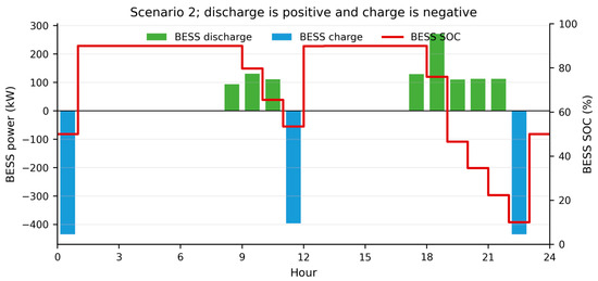
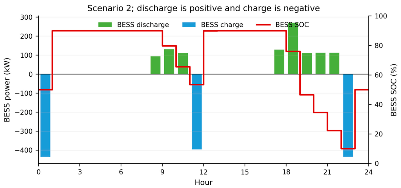
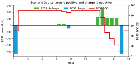
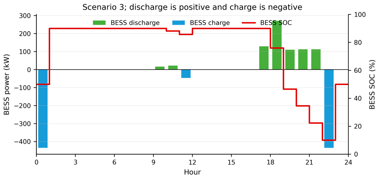
Figure 3 and Figure 4 show separate BESS charging and discharging powers and the 25-node SOC trajectories. Positive bars denote discharge and negative bars denote charging. Both S2 and S3 begin and end at 50% SOC; the minimum and maximum SOC values are 10% and 90%. No hourly interval contains simultaneous charging and discharging.

Figure 3. Scenario 2 BESS charging power, discharging power, and 25-node SOC. Positive values denote discharging, and negative values denote charging.

Figure 4. Scenario 3 BESS charging power, discharging power, and 25-node SOC. Positive values denote discharging, and negative values denote charging.

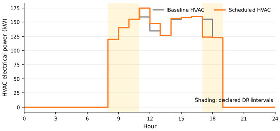
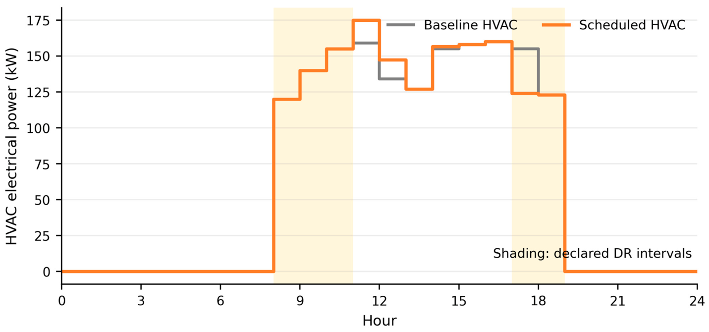
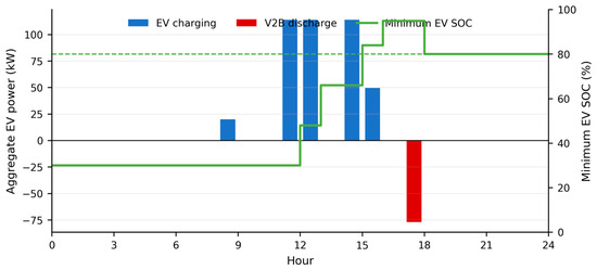
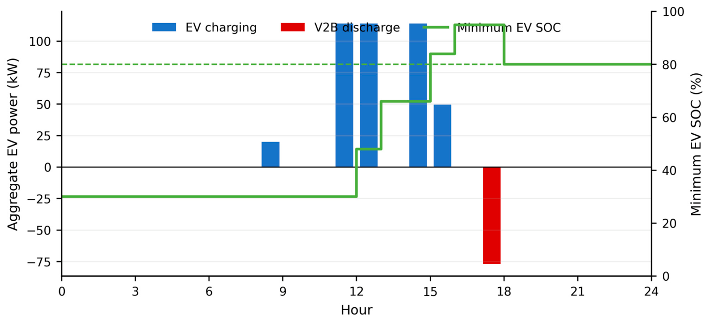
The HVAC schedule in Figure 5 shifts 31.00 kWh of electrical load away from declared response hours while recovering the same daily HVAC electrical energy. This result is an electrical-load estimate. Figure 6 shows aggregate EV charging, V2B discharge, and the minimum fleet SOC. The S3 fleet charges 411.67 kWh, discharges 76.95 kWh to the building, incurs 49.72 kWh of modeled conversion losses, and reaches 80% at departure.

Figure 5. Baseline and optimized HVAC electrical power.

Figure 6. Aggregate EV charging power, V2B discharging power, and minimum fleet SOC in Scenario 3.

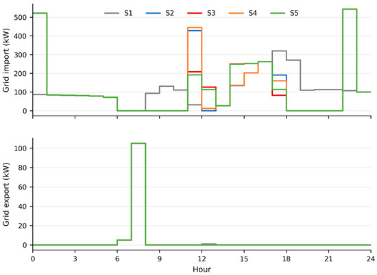
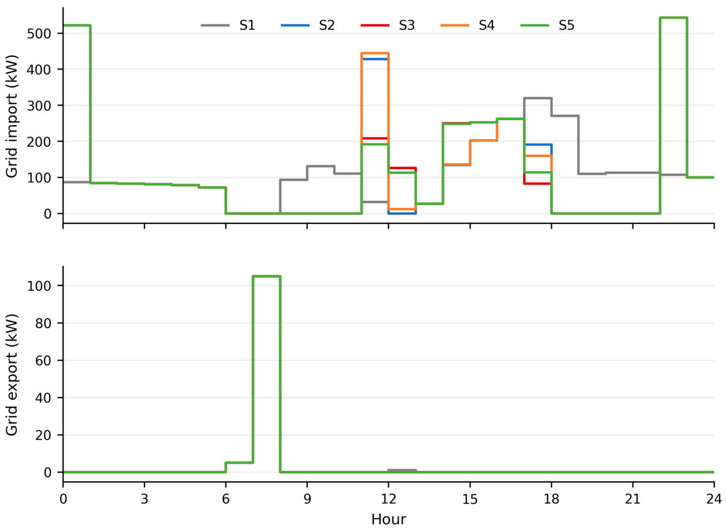
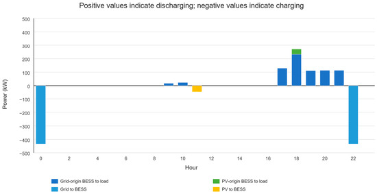
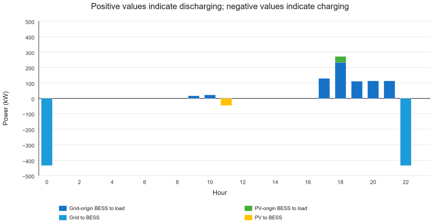
Figure 7 separates grid import and export for all five scenarios. The MILP prohibits simultaneous import and export in every interval. Figure 8 confirms that grid-origin battery energy is discharged only to building load. PV-origin BESS export is zero in the optimal base-case solutions, and all 110 kWh of S2–S5 export is direct PV.

Figure 7. Hourly grid import and export for Scenarios 1–5.

Figure 8. Scenario 3 origin-resolved BESS flows. Positive values denote BESS discharging to the building load, whereas negative values denote charging from the grid or PV.

3.2. Economic, Grid-Interaction, and Carbon Performance

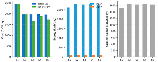
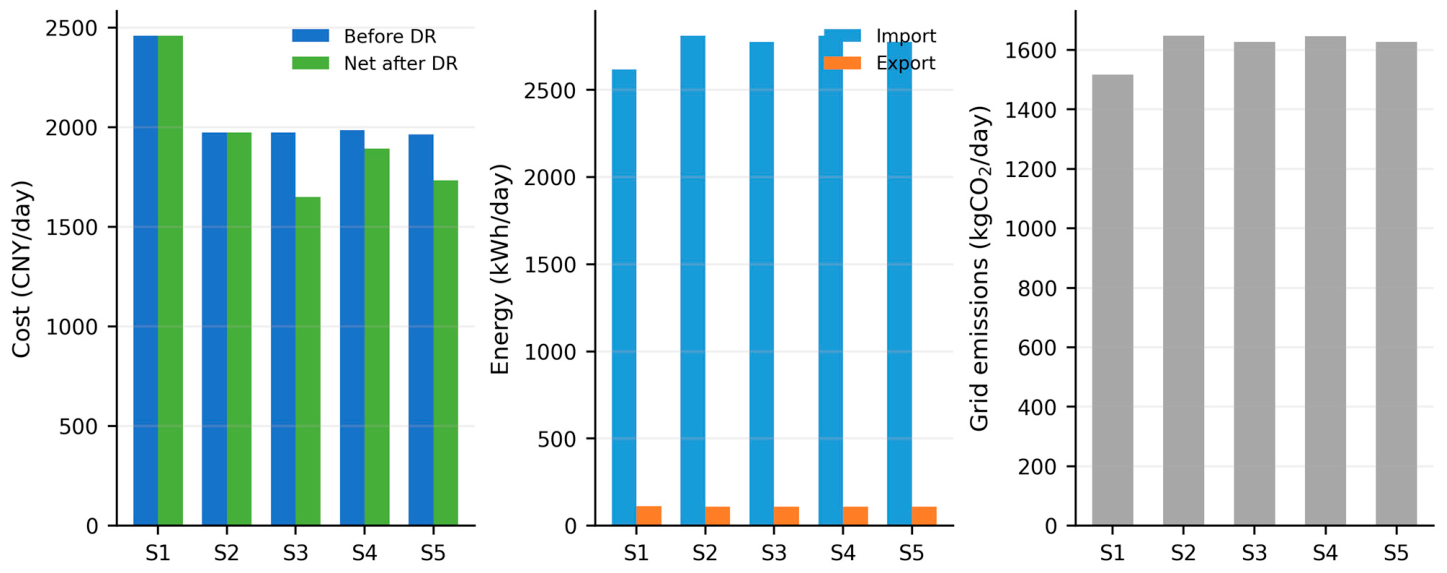
S2 reduces the selected-day operating cost from 2459.81 CNY in S1 to 1974.04 CNY, a 19.75% decrease before any DR incentive. This is a short-term dispatch difference, not an annual recurring saving. In S3, the operating cost before DR incentives is 1974.73 CNY, 0.70 CNY (0.04%) higher than S2. The 107.95 kWh verified response earns 323.85 CNY at 3 CNY/kWh, reducing the net cost to 1650.88 CNY, 16.37% below S2. Thus, the coordinated scenario’s economic superiority over S2 is policy-dependent, even though its grid import and grid-side carbon emissions are 1.27% and 1.28% lower, respectively. Table 5 shows that S3 achieves the lowest net operating cost of 1650.88 CNY after DR revenue, whereas S1 retains the lowest grid import and grid-side emissions.

Table 5. Base-scenario economic, grid-interaction, and carbon results.

Scenario	Cost Before DR (CNY)	DR Revenue (CNY)	Net Cost (CNY)	Grid Import (kWh)	Grid Export (kWh)	Grid CO2 (kg)	Peak Import (kW)
S1	2459.81	0.00	2459.81	2617.97	111.00	1517.63	320.00
S2	1974.04	0.00	1974.04	2811.50	110.00	1647.97	542.78
S3	1974.73	323.85	1650.88	2775.71	110.00	1626.90	542.78
S4	1984.98	93.00	1891.98	2811.50	110.00	1646.86	542.78
S5	1963.79	230.85	1732.94	2775.71	110.00	1628.01	542.78

The ablation results clarify the separate policy contributions. S4 attributes 31.00 kWh of verified response and 93.00 CNY of revenue to HVAC shifting; S5 attributes 76.95 kWh and 230.85 CNY to EV/V2B. Their sum equals the 107.95 kWh and 323.85 CNY in S3 because the two response resources do not overlap in the accounting constraint. S5 has a lower pre-incentive operating cost than S3 because adding the HVAC response introduces a response cost while daily HVAC energy is conserved. Figure 9 visualizes the cross-scenario trade-off: the BESS-enabled cases reduce operating cost through temporal energy shifting but increase daily grid import and emissions relative to S1. DR revenue lowers the net costs of S3–S5, while S3 and S5 also slightly reduce grid import and emissions relative to S2.

Figure 9. Base-scenario operating cost before DR incentives, net operating cost, grid import/export, and grid-side carbon emissions.

3.3. Complete Daily Energy and State Accounting

Table 6 confirms complete daily energy and state accounting.

Table 6. Complete daily energy, state, and numerical-balance accounting.

Metric	S1	S2	S3	S4	S5
PV availability (kWh)	2402.70	2402.70	2402.70	2402.70	2402.70
PV curtailment (kWh)	0.00	0.00	0.00	0.00	0.00
Grid import (kWh)	2617.97	2811.50	2775.71	2811.50	2775.71
Direct PV export (kWh)	111.00	110.00	110.00	110.00	110.00
PV-origin BESS export (kWh)	0.00	0.00	0.00	0.00	0.00
Rigid load (kWh)	3007.00	3007.00	3007.00	3007.00	3007.00
HVAC electricity (kWh)	1586.00	1586.00	1586.00	1586.00	1586.00
EV charging (kWh)	316.67	316.67	411.67	316.67	411.67
EV V2B discharge (kWh)	0.00	0.00	76.95	0.00	76.95
EV conversion losses (kWh)	31.67	31.67	49.72	31.67	49.72
BESS charging (kWh)	0.00	1266.50	916.00	1266.50	916.00
BESS discharging (kWh)	0.00	1071.97	775.30	1071.97	775.30
BESS conversion losses (kWh)	0.00	194.53	140.70	194.53	140.70
Grid-to-BESS charging (kWh)	0.00	960.50	869.57	1266.50	869.57
Grid-origin BESS-to-load (kWh)	0.00	812.97	736.00	1071.97	736.00
Initial BESS SOC (%)	N/A	50.00	50.00	50.00	50.00
Terminal BESS SOC (%)	N/A	50.00	50.00	50.00	50.00
Minimum EV departure SOC (%)	80.00	80.00	80.00	80.00	80.00
Max. hourly residual (kW)	5.68 × 10−14	5.68 × 10−14	1.14 × 10−13	1.14 × 10−13	2.27 × 10−13
Daily residual (kWh)	2.84 × 10−14	5.33 × 10−14	1.35 × 10−13	8.79 × 10−14	2.39 × 10−13

3.4. Re-Optimization-Based Sensitivity Analysis

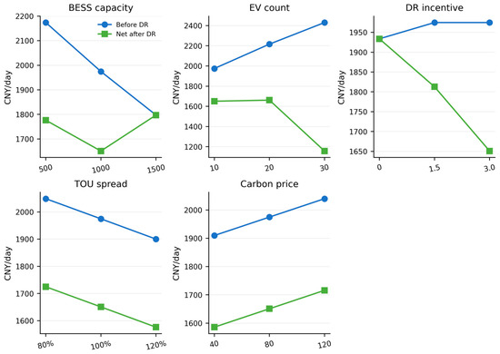
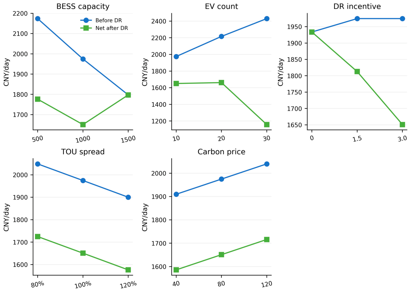
The corrected formulation permits grid import or the flexible-resource difference to exceed the Scenario 2 baseline because only their positive parts can be credited. At kDR = 0, all DR credit and sign variables are fixed to zero, so the baseline imposes no restriction. The independently optimized no-incentive Scenario 3 costs 1933.72 CNY versus 1974.04 CNY for matched Scenario 2 (Δ = −40.31 CNY). At 1.5 and 3 CNY/kWh, Scenario 3 net costs are 1812.81 and 1650.88 CNY, with matched differences of −161.23 and −323.15 CNY. Table 7 demonstrates that the economic benefit of S3 depends strongly on the matched S2 baseline.

Table 7. Matched Scenario 2 and Scenario 3 sensitivity results and direct differences.

Family	Level	S2 Net Cost (CNY)	S3 Cost Before DR (CNY)	S3 DR Revenue (CNY)	S3 Net Cost (CNY)	Δ Net cost, S3−S2 (CNY)	Δ Grid CO2, S3–S2 (kg)
BESS capacity	500 kWh	2164.66	2174.01	397.65	1776.36	−388.30	−22.37
BESS capacity	1000 kWh	1974.04	1974.73	323.85	1650.88	−323.15	−21.08
BESS capacity	1500 kWh	1837.59	1797.27	0.00	1797.27	−40.31	−27.65
EV penetration	10 EVs	1974.04	1974.73	323.85	1650.88	−323.15	−21.08
EV penetration	20 EVs	2228.78	2216.43	554.70	1661.73	−567.05	−43.82
EV penetration	30 EVs	2555.47	2430.44	1272.90	1157.54	−1397.93	−52.93
DR incentive	0 CNY/kWh	1974.04	1933.72	0.00	1933.72	−40.31	−27.65
DR incentive	1.5 CNY/kWh	1974.04	1974.73	161.92	1812.81	−161.23	−21.08
DR incentive	3.0 CNY/kWh	1974.04	1974.73	323.85	1650.88	−323.15	−21.08
TOU spread	80%	2038.72	2048.80	323.85	1724.95	−313.76	−21.08
TOU spread	100%	1974.04	1974.73	323.85	1650.88	−323.15	−21.08
TOU spread	120%	1908.89	1900.20	323.85	1576.35	−332.55	−21.08
Carbon price	40 CNY/tCO2	1908.12	1909.66	323.85	1585.81	−322.31	−21.08
Carbon price	80 CNY/tCO2	1974.04	1974.73	323.85	1650.88	−323.15	−21.08
Carbon price	120 CNY/tCO2	2039.96	2039.81	323.85	1715.96	−324.00	−21.08

Matched comparisons show that BESS capacity changes both arbitrage opportunity and the Scenario 2 DR baseline. The 1000 kWh case gives the lowest Scenario 3 net cost only among the three tested capacities; it is not a general optimum. Increasing EV penetration changes both demand and eligible response, so total costs are not interpreted as like-for-like fleet performance. Table 8 therefore reports system cost, DR revenue, and grid emissions normalized by EV count, together with matched Scenario 3−Scenario 2 differences. Table 8 and Figure 10 reveals distinct sensitivity patterns, and the complete paired absolute and normalized results are provided in Supplementary File S1.

Table 8. EV-penetration results normalized by fleet size and compared with the matched Scenario 2 baseline.

Fleet	S2 Net Cost/EV (CNY)	S3 Pre-DR Cost/EV (CNY)	S3 DR Revenue/EV (CNY)	S3 Net Cost/EV (CNY)	Δ Net Cost/EV (CNY)	S3 CO2/EV (kg)	Δ CO2/EV (kg)
10 EVs	197.40	197.47	32.38	165.09	−32.32	162.69	−2.11
20 EVs	111.44	110.82	27.73	83.09	−28.35	90.22	−2.19
30 EVs	85.18	81.01	42.43	38.58	−46.60	65.83	−1.76

Figure 10. One-factor-at-a-time re-optimization results.

3.5. BESS Investment-Cost Screening

Table 9 converts the NREL battery-pack and inverter benchmarks into a screened capital amount of 1.899 million CNY for the 1000 kWh/500 kW BESS and an annualized cost of 245,929.19 CNY, excluding replacement and balance-of-system costs.

Table 9. Separate BESS capital-cost screening calculation.

Item	Value	Scope
Battery-pack benchmark	215 USD/kWh	NREL 2024 ATB, 2 h commercial storage
Central-inverter benchmark	97.5 USD/kW	NREL 2024 ATB
Accounting exchange rate	7.2 CNY/USD	Screening assumption
Capacity	1000 kWh/500 kW	Predetermined base configuration
Screened capital amount	1,899,000 CNY	Pack + central inverter only
CRF	0.1295	$\mathrm{r}=5\%$; ${\mathrm{N}}_{\mathrm{y}}=10$ years
Annualized screening cost	245,929.19 CNY/year	Excludes replacement and BOS

4. Discussion

4.1. Physical Closure and the Role of BESS

The principal methodological correction is the removal of initial-SOC free energy. A total cyclic terminal state would prevent net depletion, but origin-specific closure is needed when only PV-origin stored energy may be exported. Assigning the initial 500 kWh to the grid-origin account and restoring both virtual accounts at hour 24 ensures that initial energy cannot be relabeled or consumed without repayment. Separate binaries also make the reported power physically interpretable.

The corrected results also show an important distinction between energy and power metrics. S2 purchases more daily grid electricity than S1 because round-trip losses and price-driven charging increase imported energy, yet it pays less because exchange is shifted toward lower-price hours. Its modeled grid emissions are consequently higher than S1 for this particular day. The BESS should therefore be described as changing the net grid-exchange profile and shifting exchange across time, not as automatically saving building energy or reducing carbon.

4.2. Technical Response, Policy Incentive

HVAC and EV/V2B coordination reduce S3 grid import and grid-side carbon emissions relative to S2. The technical pre-incentive cost, however, is 0.70 CNY higher because HVAC response and EV degradation costs offset the small energy-price benefit. The base-case economic ranking therefore changes only after DR revenue is included. S4 and S5 demonstrate that EV/V2B provides the larger response quantity under the adopted fleet and event hours, while HVAC contributes a smaller, energy-neutral timing shift.

4.3. Engineering and Research Implications

For engineering deployment, export metering and eligibility must distinguish direct PV export from stored-energy export, and charger communication must enforce the binary commands represented in the optimization. The matched BESS comparisons show that capacity affects the DR baseline and import peaks as well as cost. The 1000 kWh case performs best only among 500, 1000, and 1500 kWh under the selected inputs; capacity selection requires an investment-planning model. Likewise, EV-fleet totals combine higher mobility demand with higher incentive eligibility, so matched and per-EV indicators are required for interpretation.

The carbon-price sensitivity did not change the schedule because the price signal was small relative to tariff and other operating costs for the selected day. This does not imply that carbon-aware scheduling is ineffective in general; it shows that signal magnitude and correlation with tariff and load are decisive. Future studies should test alternative carbon-price ranges, marginal factors, and uncertain forecasts.

4.4. Limitations and Future Work

The results cover one Suzhou office-building case and one reconstructed typical summer day. Inputs are deterministic, and the study does not simulate forecast error, stochastic weather, load or EV uncertainty, real-time adaptation, communication delay, charger failure, or rolling-horizon control. Seasonal sensitivity was not performed because verified seasonal building and HVAC profiles were unavailable.

The HVAC formulation is an electrical-load approximation, not a calibrated RC or physics-based building model. It does not calculate indoor temperature, solar or internal gains, thermal-zone heterogeneity, occupant-dependent comfort, or complete post-response rebound, and it has no measured indoor-temperature validation. Consequently, the study does not claim that comfort is maintained.

EV arrival, departure, connection, initial SOC, charger availability, and target SOC are fixed. The export rule is a conservative modeling assumption; actual market restrictions, settlement, and metering require project-specific verification. Battery degradation is represented only by a linear throughput charge, while calendar aging and state-dependent degradation are omitted. The BESS CAPEX screen is not a full lifecycle assessment and excludes several project costs.

Although the model closes the terminal BESS state and tracks energy origin, a single day cannot establish annual performance, recurring savings, investment payback, or universal optimality. Future work should use measured multi-season building data, calibrated thermal dynamics, probabilistic EV behavior, rolling multi-day states, detailed degradation and investment models, and field implementation tests.

5. Conclusions

An auditable deterministic day-ahead MILP was developed for a PV-storage office building with simplified HVAC electrical response and EV/V2B. The formulation uses separate nonnegative charging and discharging variables, binary mutual-exclusion states, 24 power intervals and 25 state nodes, a cyclic 50% BESS terminal SOC, PV/grid virtual energy accounts, and exact positive-part DR verification. Optimized imports may exceed the matched baseline; only positive verified reductions are credited, and the DR block is fully deactivated at zero incentive. All 35 runs are supplied with hourly inputs, coefficients, code, solver logs, and outputs.

For the selected typical summer day, the PV-only and BESS-only operating costs are 2459.81 and 1974.04 CNY. The coordinated S3 cost before DR incentives is 1974.73 CNY; its 323.85 CNY incentive reduces net cost to 1650.88 CNY. Relative to S2, S3 lowers grid import and grid-side carbon emissions by 1.27% and 1.28%, but its pre-incentive cost is 0.04% higher. The corrected DR equations leave these optima unchanged because the former unintended bounds were nonbinding. HVAC-only and EV-only ablations attribute 31.00 and 76.95 kWh of credited response, respectively. The 1000 kWh BESS gives the lowest S3 net cost among the three tested capacities, and EV-penetration totals must be read against matched S2 and per-EV indicators.

All BESS scenarios return to 50% SOC and all EVs reach at least 80% departure SOC. These are optimization feasibility results.

Appendix A.1. Variable Domains and State Boundaries

All continuous flow variables are nonnegative unless an explicitly defined net quantity is used only for reporting. The two BESS energy-origin accounts are separately nonnegative at every state node. The following domain statement supplements Equations (1)–(15).

$$\begin{array}{c}{\mathrm{E}}_{\mathrm{B}\mathrm{E}\mathrm{S}\mathrm{S},\mathrm{n}}^{\mathrm{P}\mathrm{V}}\ge 0,{\mathrm{E}}_{\mathrm{B}\mathrm{E}\mathrm{S}\mathrm{S},\mathrm{n}}^{\mathrm{g}\mathrm{r}\mathrm{i}\mathrm{d}}\ge 0,\mathrm{n}\in N\\ {\mathrm{P}}_{\mathrm{B}\mathrm{E}\mathrm{S}\mathrm{S},\mathrm{t}}^{\mathrm{c}\mathrm{h}},{\mathrm{P}}_{\mathrm{B}\mathrm{E}\mathrm{S}\mathrm{S},\mathrm{t}}^{\mathrm{d}\mathrm{i}\mathrm{s}},{\mathrm{P}}_{\mathrm{g}\mathrm{r}\mathrm{i}\mathrm{d},\mathrm{t}}^{\mathrm{b}\mathrm{u}\mathrm{y}},{\mathrm{P}}_{\mathrm{g}\mathrm{r}\mathrm{i}\mathrm{d},\mathrm{t}}^{\mathrm{s}\mathrm{e}\mathrm{l}\mathrm{l}}\ge 0\\ {\mathrm{P}}_{\mathrm{E}\mathrm{V},\mathrm{i},\mathrm{t}}^{\mathrm{c}\mathrm{h}},{\mathrm{P}}_{\mathrm{E}\mathrm{V},\mathrm{i},\mathrm{t}}^{\mathrm{d}\mathrm{i}\mathrm{s}},{\mathrm{P}}_{\mathrm{H}\mathrm{V}\mathrm{A}\mathrm{C},\mathrm{t}},{\mathrm{P}}_{\mathrm{D}\mathrm{R},\mathrm{t}}\ge 0\end{array}$$

Each EV arrives at node 8 with 30% SOC. Its SOC is bounded between 10% and 95%, it must reach at least 80% at departure node 18, and its state is fixed at the initial value before arrival and propagated without charging or discharging after departure.

$$\begin{array}{c}{\mathrm{S}\mathrm{O}\mathrm{C}}_{\mathrm{E}\mathrm{V},\mathrm{i}}^{\mathrm{m}\mathrm{i}\mathrm{n}}\le {\mathrm{S}\mathrm{O}\mathrm{C}}_{\mathrm{E}\mathrm{V},\mathrm{i},\mathrm{n}}\le {\mathrm{S}\mathrm{O}\mathrm{C}}_{\mathrm{E}\mathrm{V},\mathrm{i}}^{\mathrm{m}\mathrm{a}\mathrm{x}}\\ {\mathrm{S}\mathrm{O}\mathrm{C}}_{\mathrm{E}\mathrm{V},\mathrm{i},8}={\mathrm{S}\mathrm{O}\mathrm{C}}_{\mathrm{E}\mathrm{V},\mathrm{i}}^{\mathrm{i}\mathrm{n}\mathrm{i}\mathrm{t}}=0.30\\ {\mathrm{S}\mathrm{O}\mathrm{C}}_{\mathrm{E}\mathrm{V},\mathrm{i},18}\ge {\mathrm{S}\mathrm{O}\mathrm{C}}_{\mathrm{E}\mathrm{V},\mathrm{i}}^{\mathrm{t}\mathrm{a}\mathrm{r}\mathrm{g}\mathrm{e}\mathrm{t}}=0.80\\ {\mathrm{a}}_{\mathrm{i},\mathrm{t}}=0\Rightarrow {\mathrm{P}}_{\mathrm{E}\mathrm{V},\mathrm{i},\mathrm{t}}^{\mathrm{c}\mathrm{h}}={\mathrm{P}}_{\mathrm{E}\mathrm{V},\mathrm{i},\mathrm{t}}^{\mathrm{d}\mathrm{i}\mathrm{s}}=0\end{array}$$

Appendix A.2. HVAC Variable Domains and Flexibility Window

The downward-response and recovery variables are nonnegative. HVAC flexibility is enabled only for intervals 8–18 inclusive; outside this window the scheduled HVAC power equals the baseline and both response variables are fixed to zero. The daily recovery equality in Equation (24) applies whenever HVAC flexibility is enabled.

$$\begin{array}{c}\Delta {\mathrm{P}}_{\mathrm{H}\mathrm{V}\mathrm{A}\mathrm{C},\mathrm{t}}^{\mathrm{d}\mathrm{o}\mathrm{w}\mathrm{n}}\ge 0,\Delta {\mathrm{P}}_{\mathrm{H}\mathrm{V}\mathrm{A}\mathrm{C},\mathrm{t}}^{\mathrm{u}\mathrm{p}}\ge 0\\ {\mathcal{T}}_{\mathrm{H}\mathrm{V}\mathrm{A}\mathrm{C}}=\{8,\dots ,18\}\end{array}$$

Appendix A.3. Objective-Function Aggregate Quantities

The four aggregate energy quantities in Equation (31) are computed directly from hourly decision variables as follows; no additional estimated term is used.

$$\begin{array}{c}{\mathrm{E}}_{\mathrm{P}\mathrm{V},\mathrm{u}\mathrm{s}\mathrm{e}\mathrm{d}}={\displaystyle \sum _{\mathrm{t}\in \mathcal{T}}}{\mathrm{P}}_{\mathrm{P}\mathrm{V}\to \mathrm{l}\mathrm{o}\mathrm{a}\mathrm{d},\mathrm{t}}+{\mathrm{P}}_{\mathrm{P}\mathrm{V}\to \mathrm{B}\mathrm{E}\mathrm{S}\mathrm{S},\mathrm{t}}+{\mathrm{P}}_{\mathrm{P}\mathrm{V},\mathrm{s}\mathrm{e}\mathrm{l}\mathrm{l},\mathrm{t}}\mathsf{\Delta }\mathrm{t}\\ {\mathrm{E}}_{\mathrm{B}\mathrm{E}\mathrm{S}\mathrm{S},\mathrm{t}\mathrm{h}\mathrm{r}\mathrm{o}\mathrm{u}\mathrm{g}\mathrm{h}}={\displaystyle \sum _{\mathrm{t}\in \mathcal{T}}}{\mathrm{P}}_{\mathrm{B}\mathrm{E}\mathrm{S}\mathrm{S},\mathrm{t}}^{\mathrm{c}\mathrm{h}}+{\mathrm{P}}_{\mathrm{B}\mathrm{E}\mathrm{S}\mathrm{S},\mathrm{t}}^{\mathrm{d}\mathrm{i}\mathrm{s}}\mathsf{\Delta }\mathrm{t}\\ {\mathrm{E}}_{\mathrm{H}\mathrm{V}\mathrm{A}\mathrm{C},\mathrm{d}\mathrm{o}\mathrm{w}\mathrm{n}}={\displaystyle \sum _{\mathrm{t}\in \mathcal{T}}}\mathsf{\Delta }{\mathrm{P}}_{\mathrm{H}\mathrm{V}\mathrm{A}\mathrm{C},\mathrm{t}}^{\mathrm{d}\mathrm{o}\mathrm{w}\mathrm{n}}\mathsf{\Delta }\mathrm{t}\\ {\mathrm{E}}_{\mathrm{E}\mathrm{V},\mathrm{V}2\mathrm{B}}={\displaystyle \sum _{\mathrm{i}\in \mathcal{I},\mathrm{t}\in \mathcal{T}}}{\mathrm{P}}_{\mathrm{E}\mathrm{V},\mathrm{i},\mathrm{t}}^{\mathrm{d}\mathrm{i}\mathrm{s}}\mathsf{\Delta }\mathrm{t}\end{array}$$

Appendix A.4. Scenario-Specific Deactivation Constraints

Table A1 gives the exact switches used in the executable model. For every flexible scenario with a positive incentive, Equations (28)–(30) are active. When the incentive coefficient is zero, the credited-response variable, both positive-part auxiliaries, and both sign binaries are fixed to zero; the matched S2 baseline is retained only for reporting and imposes no constraint on the schedule.

Table A1. Scenario activation and deactivation rules.

Scenario	BESS	HVAC Response	EV Flexibility	V2B	DR Accounting
S1	All BESS flows and states deactivated	HVAC = baseline	Fixed charging	Off	Off
S2	Active	HVAC = baseline	Fixed charging	Off	Off; supplies baseline
S3	Active	Active, t = 8, …, 18	Active while connected	Active	Active if kDR > 0
S4	Active	Active, t = 8, …, 18	Fixed charging	Off	Active if kDR > 0
S5	Active	HVAC = baseline	Active while connected	Active	Active if kDR > 0

Table A1. Scenario activation and deactivation rules.

Scenario	BESS	HVAC Response	EV Flexibility	V2B	DR Accounting
S1	All BESS flows and states deactivated	HVAC = baseline	Fixed charging	Off	Off
S2	Active	HVAC = baseline	Fixed charging	Off	Off; supplies baseline
S3	Active	Active, t = 8, …, 18	Active while connected	Active	Active if kDR > 0
S4	Active	Active, t = 8, …, 18	Fixed charging	Off	Active if kDR > 0
S5	Active	HVAC = baseline	Active while connected	Active	Active if kDR > 0

References

- Raziei, S.A.; Mohsenian-Rad, H. Optimal demand response capacity of automatic lighting control. In Proceedings of the IEEE PES Innovative Smart Grid Technologies Conference, Washington, DC, USA, 24–27 February 2013; IEEE: New York, NY, USA, 2013; pp. 1–6. [Google Scholar]
- Sehar, F.; Pipattanasomporn, M.; Rahman, S. An energy management model to study energy and peak power savings from PV and storage in demand-responsive buildings. Appl. Energy 2016, 173, 406–417. [Google Scholar] [CrossRef] [Scilit]
- Sha’aban, Y.A.; Ikpehai, A.; Adebisi, B.; Rabie, K.M.; Gacanin, H. Bi-directional coordination of plug-in electric vehicles with economic model predictive control. Energies 2017, 10, 1507. [Google Scholar] [CrossRef] [Scilit]
- Cai, J.; Braun, J.E. Assessments of demand response potential in small commercial buildings across the United States. Sci. Technol. Built Environ. 2019, 25, 1437–1455. [Google Scholar] [CrossRef] [Scilit]
- Braun, J.E.; Lawrence, T.M.; Klaassen, C.J.; House, J.M. Demonstration of load shifting and peak-load reduction with control of building thermal mass. In Commercial Buildings: Technologies, Design, Performance Analysis, and Building Industry Trends; ASHRAE: Pacific Grove, CA, USA, 2002; pp. 55–67. [Google Scholar]
- Xu, P.; Haves, P.; Piette, M.A.; Braun, J.E. Peak demand reduction from pre-cooling with zone-temperature reset in an office building. In Proceedings of the ACEEE Summer Study on Energy Efficiency in Buildings, Pacific Grove, CA, USA, 22–27 August 2004; pp. 1–11. [Google Scholar]
- Morgan, S.; Krarti, M. Impact of electricity-rate structures on energy-cost savings of pre-cooling controls for office buildings. Build. Environ. 2007, 42, 2810–2818. [Google Scholar] [CrossRef] [Scilit]
- Liu, G.; Tomsovic, K. Robust unit commitment considering uncertain demand response. Electr. Power Syst. Res. 2015, 119, 126–137. [Google Scholar] [CrossRef] [Scilit]
- Meng, F.; Ma, Q.; Liu, Z.; Zhang, L. Multiple dynamic pricing for demand response with adaptive clustering-based customer segmentation in smart grids. Appl. Energy 2023, 333, 120626. [Google Scholar] [CrossRef] [Scilit]
- Fochesato, M.; Cenedese, C.; Lygeros, J. A Stackelberg game for incentive-based demand response in energy markets. In Proceedings of the 2022 IEEE 61st Conference on Decision and Control, Cancun, Mexico, 6–9 December 2022; IEEE: New York, NY, USA, 2022; pp. 2487–2492. [Google Scholar]
- Dranka, G.G.; Ferreira, P. Review and assessment of the different categories of demand response potentials. Energy 2019, 179, 280–294. [Google Scholar] [CrossRef] [Scilit]
- Widergren, S.; Marinovici, C.; Berliner, T.; Graves, A. Real-time pricing demand response in operations. In Proceedings of the 2012 IEEE Power and Energy Society General Meeting, San Diego, CA, USA, 22–26 July 2012; IEEE: New York, NY, USA, 2012; pp. 1–5. [Google Scholar]
- Wang, Z.; Lu, B.; Wang, B.; Qiu, Y.; Shi, H.; Zhang, B.; Li, J.; Li, H.; Zhao, W. Incentive-based emergency demand response effectively reduces peak load during heatwave without harm to vulnerable groups. Nat. Commun. 2023, 14, 6202. [Google Scholar] [CrossRef] [Scilit] [PubMed]
- Wang, R.; Xin, X.; Liu, J.; Lu, S.; Sun, Y.; Zhao, W. Quantitative method and influencing-factors analysis of demand-response performance of air-conditioning load with rebound effect. Build. Simul. 2025, 18, 295–320. [Google Scholar]
- Hurtado, L.A.; Syed, A.; Nguyen, P.H.; Kling, W.L. Multi-agent-based electric-vehicle charging method for smart-grid/smart-building energy management. In Proceedings of the 2015 IEEE Eindhoven PowerTech, Eindhoven, The Netherlands, 29 June–2 July 2015; IEEE: New York, NY, USA, 2015; pp. 1–6. [Google Scholar]
- Barone, G.; Buonomano, A.; Calise, F.; Forzano, C.; Palombo, A. Building-to-vehicle-to-building concept toward a novel zero-energy paradigm: Modelling and case studies. Renew. Sustain. Energy Rev. 2019, 101, 625–648. [Google Scholar] [CrossRef] [Scilit]
- Zhou, X.; Yap, E.W.; Dou, W.; Huang, M.; Aziz, M.S.; Robinson, D.A.; McDowell, C.; White, S.D.; Goldsworthy, M.; Sethuvenkatraman, S.; et al. Demand flexibility characterisation in non-residential buildings: A review. Appl. Energy 2025, 393, 126100. [Google Scholar] [CrossRef] [Scilit]
- Li, C.; Langner, F.; Förderer, K.; Matthes, J.; Hagenmeyer, V. A survey on the current state of demand response implementations: Models and approaches. SIGENERGY Energy Inform. Rev. 2025, 5, 12–24. [Google Scholar] [CrossRef] [Scilit]
- Marszal-Pomianowska, A.; Graf, C.; Schaffer, M.; Christensen, T.H.; Nastasi, B.; Felsmann, C.; Motoasca, E.; Guelpa, E.; Johra, H.; Leusbrock, I.; et al. Demand Management of Buildings in Thermal Networks: Collaboration Models—Overview of Involved Actors, Existing Practices, Potential Barriers and Limitations, Recommendations; Aalborg University: Aalborg, Denmark, 2025. [Google Scholar] [CrossRef] [Scilit]
- Wamalwa, F.; Ishimwe, A. Optimal energy management in a grid-tied solar PV–battery microgrid for a public building under demand response. Energy Rep. 2024, 12, 3718–3731. [Google Scholar] [CrossRef] [Scilit]
- Liao, W.; Xiao, F.; Li, Y.; Zhang, H.; Peng, J. A comparative study of demand-side energy-management strategies for building-integrated photovoltaics–battery and electric vehicles in diversified building communities. Appl. Energy 2024, 361, 122881. [Google Scholar] [CrossRef] [Scilit]
- Jin, B.; Liu, Z. Evaluating the impact of virtual energy storage under air-conditioning and building coupling on the performance of a grid-connected distributed energy system. J. Build. Eng. 2024, 89, 109309. [Google Scholar] [CrossRef] [Scilit]
- Du, B.; Jia, H.; Zhang, B.; Li, Y.; Wang, H.; Yan, J.; Du, E.; Zhang, N. Evaluating the carbon-emission-reduction potential of employing low-carbon demand response to guide electric-vehicle charging: A Chinese case study. Appl. Energy 2025, 397, 126196. [Google Scholar] [CrossRef] [Scilit]
- Li, J.; Xu, W.; Li, J.; Huang, S.; Li, Z.; Qiao, B.; Yang, C.; Sun, D.; Zhang, G. Heat extraction model and characteristics of coaxial deep borehole heat exchanger. Renew. Energy 2021, 169, 738–751. [Google Scholar] [CrossRef] [Scilit]
- Zhao, B.; Cao, X.; Zhang, S.; Ren, J.; Li, J. Day-ahead energy management of a smart-building energy system aggregated with electric vehicles based on distributionally robust optimization. Build. Simul. 2025, 18, 339–352. [Google Scholar] [CrossRef] [Scilit]
- Xu, X.; Fu, Y.; Luo, Y. Building energy flexibility with battery energy storage system: A comprehensive review. Discov. Mech. Eng. 2022, 1, 4. [Google Scholar] [CrossRef] [Scilit]
- Hoyt, T.; Arens, E.; Zhang, H. Extending air-temperature setpoints: Simulated energy savings and design considerations for new and retrofit buildings. Build. Environ. 2015, 88, 89–96. [Google Scholar] [CrossRef] [Scilit]
- Liu, X.; Sun, H.; Han, S.; Niu, S.; Qin, W.; Sun, P.; Song, D. A data-mining study of office-building energy patterns based on time-series energy-consumption data. Energy Build. 2022, 259, 111888. [Google Scholar]
- Allen, J.; Halberstadt, A.; Powers, J.; El-Farra, N.H. An optimization-based supervisory control and coordination approach for solar–load balancing in building energy management. Mathematics 2020, 8, 1215. [Google Scholar] [CrossRef] [Scilit]
- Blatiak, A.; Bellizio, F.; Badesa, L.; Strbac, G. Value of optimal trip and charging scheduling of commercial electric-vehicle fleets with vehicle-to-grid in future low-inertia systems. Sustain. Energy Grids Netw. 2022, 31, 100738. [Google Scholar] [CrossRef] [Scilit]
- Abeywardana, D.B.W.; Hredzak, B.; Agelidis, V.G.; Demetriades, G.D. Supercapacitor sizing method for energy-controlled filter-based hybrid energy-storage systems. IEEE Trans. Power Electron. 2017, 32, 1626–1637. [Google Scholar] [CrossRef] [Scilit]
- Li, Y.; Zhang, S.; Li, W.; Liu, Y.; Qin, Y.; Wei, H.; Kang, C.; Zhang, N.; Du, E. High temporal and spatial resolution projected electricity carbon-emission factors of China from 2025–2060. Sci. Data 2026, 13, 926. [Google Scholar] [CrossRef] [Scilit] [PubMed]
- Jiangsu Provincial Development and Reform Commission. Jiangsu Electric-Power Demand Response Implementation Rules; Jiangsu Provincial Development and Reform Commission: Nanjing, China, 2024. Available online: https://www.js.gov.cn/art/2024/7/25/art_64797_11305791.html (accessed on 29 July 2026).
- Jiangsu Provincial People’s Government. Archived Jiangsu Distributed-PV Green-Electricity Settlement Information; Jiangsu Provincial People’s Government: Nanjing, China, 2024. Available online: https://www.jiangsu.gov.cn/art/2024/5/14/art_88959_11250913.html (accessed on 29 July 2026).
- National Renewable Energy Laboratory (NREL). Commercial Battery Storage. In 2024 Annual Technology Baseline (ATB). Available online: https://atb.nrel.gov/electricity/2024/commercial_battery_storage (accessed on 29 July 2026).
Disclaimer/Publisher’s Note: The statements, opinions and data contained in all publications are solely those of the individual author(s) and contributor(s) and not of MDPI and/or the editor(s). MDPI and/or the editor(s) disclaim responsibility for any injury to people or property resulting from any ideas, methods, instructions or products referred to in the content. |
© 2026 by the authors. Licensee MDPI, Basel, Switzerland. This article is an open access article distributed under the terms and conditions of the Creative Commons Attribution (CC BY) license.