Incipient Interturn Short-Circuit Fault Diagnosis of Permanent Magnet Motors Based on Multiscale Entropy and Topological Data Analysis

Abstract

Incipient stator interturn short-circuit faults in permanent magnet synchronous motors produce only weak changes in the terminal currents, which limits the sensitivity of conventional amplitude- and unbalance-based indicators. This paper proposes a phase-wise diagnostic framework that combines multiscale sample entropy (MSE), topological data analysis (TDA), and a Gaussian mixture model (GMM). For each three-period current window, ten scale-dependent sample-entropy components and two persistent-entropy components are concatenated into a 12-dimensional feature vector. A separate GMM is trained for each phase using healthy data only. The resulting likelihood-based health scores are used for fault detection and faulty-phase localization, while physically defined score boundaries calibrated from measured short-circuit-current groups are used for severity assessment. Experiments on a 1.5 kW, 8-pole, 12-slot PMSM demonstrate class-wise recalls of 96.50–100% and an overall accuracy of 97.50% under the investigated operating conditions. The results show that the combined temporal and topological representation can reveal weak current changes that are difficult to distinguish using conventional terminal-current indicators.

1. Introduction

With the pursuit of high-efficiency and low-carbon electromechanical systems, permanent magnet synchronous motors (PMSMs) have been increasingly adopted in electric transportation and industrial automation because of their high power density, efficiency, wide speed range, and precise torque control. Reliability is particularly important in traction applications, where high vehicle inertia and limited tolerance for unplanned shutdown constrain maintenance and fault-handling options. Unlike an electrically excited rotor, a permanent-magnet rotor continues to produce magnetic excitation while rotating even after the stator supply is interrupted. A winding fault can therefore remain electromagnetically active until the rotor stops. PMSM faults include mechanical faults, winding and insulation faults, and permanent-magnet faults. Winding damage remains a non-negligible failure mode in synchronous machines [1]. An interturn short-circuit fault (ISCF) is particularly safety-critical because the resulting circulating current produces localized heating and may propagate into phase-to-phase or phase-to-ground faults. Consequently, timely detection of an incipient ISCF is important for preventing fault propagation and improving the operational safety of PMSM drive systems.

Existing ISCF diagnostic methods for permanent magnet synchronous motors can be broadly divided into model-based, signal-processing-based, and data-driven methods [2]. Model-based methods compare measured quantities with a healthy or faulty machine model [3,4,5]. They provide physically interpretable indicators, but their accuracy depends on parameter knowledge and on the fidelity of the adopted model. Recent observer- and multiple-model-based studies have improved fault-resistance estimation and online detection [6]; nevertheless, model adaptation remains necessary when machine parameters and operating points vary.

Signal-processing methods extract fault-sensitive quantities from measured voltages, currents, speed, torque, or vibration signals [7,8,9]. Representative indicators include zero-sequence voltage [10], high-frequency injection responses [11,12], negative-sequence current [13], and rotor-speed signatures [14]. Entropy-based processing has also been introduced to characterize weak nonstationary changes. For example, a 2024 study combined optimized variational mode decomposition with multiscale fuzzy entropy for interturn-fault diagnosis in a fractional-slot permanent-magnet machine [15]. These methods are generally interpretable and can be implemented with limited training data, but a single amplitude, spectral, or entropy descriptor may not fully represent the weak dynamical changes associated with an incipient high-resistance fault.

Recent AI-driven studies have used convolutional, recurrent, attention, transformer, physical–data dual, and meta-learning architectures to improve fault classification under complex conditions [16,17,18]. Their main advantage is the ability to learn nonlinear discriminative representations from multi-condition data. However, the reported performance commonly depends on labelled fault samples, simulation-assisted training, and a training distribution that covers the expected fault severities and operating conditions. These requirements can limit deployment when destructive fault data are scarce.

Topological data analysis has recently been explored in rotating-machinery condition monitoring because persistent homology can summarize the geometry of a reconstructed trajectory across multiple proximity scales. Recent bearing-diagnosis results indicate that topological descriptors can complement conventional statistical features when the number of fault samples is limited [19]. Nevertheless, applications of persistent homology to phase-wise PMSM interturn-fault diagnosis remain limited, and the relationship between the topological quantities and experimentally measured current windows is often not stated explicitly.

The present work addresses this gap by combining two complementary, manually interpretable representations of each phase current. MSE retains the scale-dependent irregularity of the waveform, whereas TDA summarizes the connected-component and loop-lifetime distributions of the delay-coordinate point cloud. The fused feature vector is evaluated by phase-specific GMMs trained with healthy data only. Fault severity is not represented by additional class-conditional GMMs; instead, it is assigned by score boundaries calibrated against the measured short-circuit-current groups. This design reduces the amount of labelled fault data required for model construction while retaining a physically traceable severity definition.

The main contributions are as follows:

• A phase-domain analytical model is developed to relate the internal short-circuit current to the measurable three-phase current perturbations. The model shows why the directly faulted phase deviates more strongly than the other two phases and why the terminal-current change remains weak at the incipient stage.
• A reproducible phase-wise feature-extraction procedure is established. Ten scale-dependent sample-entropy values and two persistent-entropy values are calculated from the same three-period current window. Their experimental interpretation is linked explicitly to the waveforms, delay-coordinate projections, persistence intervals, and fused features.
• A one-class healthy-distribution model is constructed for each phase using GMMs trained only with healthy features. The likelihood scores are used for health assessment and phase localization. Mild, moderate, and severe levels are assigned through a separate calibration based on the measured fault-loop current, rather than by fitting four supervised class densities.

2. Interturn Short-Circuit Fault in PMSM

The interturn short-circuit fault (ISCF) remains safety-critical because the magnetic field produced by the permanent-magnet rotor cannot be de-energized during rotation. Once the insulation between adjacent or non-adjacent turns is damaged, a closed conductive loop is formed within the stator winding. The permanent-magnet flux continuously induces an electromotive force in this loop, resulting in a circulating current, localized heating, and accelerated insulation degradation. If the fault is not detected at an early stage, it may propagate into a phase-to-phase or phase-to-ground short circuit and may also cause irreversible demagnetization, increased torque ripple, vibration, and noise.

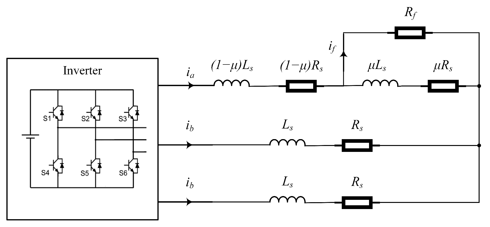
As illustrated in Figure 1, an ISCF is assumed to occur in Phase A. The shorted-turn ratio is defined as

$$\mu ={\displaystyle \frac{N_f}{N_{total}}},$$

(1)

where $N_f$ is the number of shorted turns and $N_{\mathrm{total}}$ is the total number of turns in one phase.

The residual insulation resistance at the short-circuit point is denoted by $R_f$. A large $R_f$ represents an incipient high-resistance insulation fault, whereas $R_f\to 0$ corresponds to a nearly metallic short circuit. The shorted-turn ratio $\mu$ and the residual insulation resistance $R_f$ jointly determine the induced short-circuit current and the resulting variation of the measurable stator currents.

2.1. Phasor-Domain Model and Assumptions

To reveal the relationship between the internal short-circuit current and the externally measured three-phase currents, a fundamental-frequency phasor model is established. The following assumptions are adopted:

• The motor operates in a quasi-steady state within one diagnostic window, and the electrical angular frequency ${\omega }_e$ is approximately constant.
• The healthy portions of the three-phase windings are symmetric.
• The motor is connected as a three-wire star-connected system, and therefore the phase currents satisfy $I_a+I_b+I_c=0$.
• Magnetic saturation, slotting effects, parameter variation with temperature, and high-frequency switching components are neglected in the fundamental-frequency analytical model.
• The ISCF is localized in Phase A. The mutual couplings between the shorted section and Phases B and C are retained in the general model and neglected only when deriving the simplified closed-form expressions.

All voltages and currents in this section are represented by RMS phasors. The three-phase voltage, back-electromotive-force, and current vectors are defined as

$$\mathbf{U}={\left[\begin{array}{ccc}{U}_a& U_b& U_c\end{array}\right]}^{\mathrm{T}},\mathbf{E}={\left[\begin{array}{ccc}{E}_a& E_b& E_c\end{array}\right]}^{\mathrm{T}},$$

(2)

and

$$\mathbf{I}={\left[\begin{array}{ccc}{I}_a& I_b& I_c\end{array}\right]}^{\mathrm{T}}.$$

(3)

For a symmetrical PMSM, the phase-domain stator impedance matrix is expressed as

$${\mathbf{Z}}_s=\left[\begin{array}{ccc}{Z}_p& Z_m& Z_m\\ Z_m& Z_p& Z_m\\ Z_m& Z_m& Z_p\end{array}\right],$$

(4)

where

$$Z_p=R_s+\mathrm{j}{\omega }_e{L}_s,Z_m=\mathrm{j}{\omega }_{e}M.$$

(5)

Here, $R_s$ and $L_s$ are the phase resistance and self-inductance, respectively, and M is the algebraic mutual inductance between two phases.

Because the neutral point is not externally connected, the zero-sequence component is eliminated using the projection matrix

$$\mathbf{P}={\mathbf{I}}_3-{\displaystyle \frac{1}{3}}\mathbf{1}{\mathbf{1}}^{\mathrm{T}}={\displaystyle \frac{1}{3}}\left[\begin{array}{ccc}2& -1& -1\\ -1& 2& -1\\ -1& -1& 2\end{array}\right],$$

(6)

where

$$\mathbf{1}={\left[\begin{array}{ccc}1& 1& 1\end{array}\right]}^{\mathrm{T}}.$$

(7)

For any current vector satisfying ${\mathbf{1}}^{\mathrm{T}}\mathbf{I}=0$, the stator impedance matrix reduces to the positive- and negative-sequence impedance

$$Z_1=Z_p-Z_m=R_s+\mathrm{j}{\omega }_e(L_s-M).$$

(8)

2.2. Three-Phase Currents Under Healthy Operation

Under healthy operation, the projected phase-domain voltage equation is

$$\mathbf{P}\left(\mathbf{U}-\mathbf{E}\right)=Z_1{\mathbf{I}}_{\mathrm{H}},$$

(9)

where

$${\mathbf{I}}_{\mathrm{H}}={\left[\begin{array}{ccc}{I}_{a,\mathrm{H}}& I_{b,\mathrm{H}}& I_{c,\mathrm{H}}\end{array}\right]}^{\mathrm{T}}$$

(10)

is the healthy three-phase current vector. Therefore,

$${\mathbf{I}}_{\mathrm{H}}={\displaystyle \frac{1}{Z_1}}\mathbf{P}\left(\mathbf{U}-\mathbf{E}\right)$$

(11)

For balanced sinusoidal operation, let

$$a=\exp \left(\mathrm{j}{\displaystyle \frac{2\pi }{3}}\right),\mathbf{c}={\left[\begin{array}{ccc}1& a^2& a\end{array}\right]}^{\mathrm{T}}.$$

(12)

The balanced terminal-voltage and back-EMF vectors can then be written as

$$\mathbf{U}=U_1\mathbf{c},\mathbf{E}=E_1\mathbf{c}.$$

(13)

Since $\mathbf{P}\mathbf{c}=\mathbf{c}$, the healthy current vector becomes

$${\mathbf{I}}_{\mathrm{H}}=I_1{\left[\begin{array}{ccc}1& a^2& a\end{array}\right]}^{\mathrm{T}}$$

(14)

where

$$I_1={\displaystyle \frac{U_1-E_1}{Z_1}}.$$

(15)

Consequently,

$$I_{a,\mathrm{H}}=I_1,I_{b,\mathrm{H}}=a^2{I}_1,I_{c,\mathrm{H}}=a{I}_1.$$

(16)

Equation (16) shows that the healthy current system contains only a balanced positive-sequence component.

2.3. Fault-State Current Model

When an ISCF occurs in Phase A, the short-circuit loop is electromagnetically coupled with the three stator phases. The coupling-impedance vector is defined as

$$\mathbf{q}=\left[\begin{array}{c}{z}_{af}\\ z_{bf}\\ z_{cf}\end{array}\right]=\left[\begin{array}{c}-\mu R_s+\mathrm{j}{\omega }_e{L}_f\\ -\mathrm{j}{\omega }_e{M}_{af-b}\\ -\mathrm{j}{\omega }_e{M}_{af-c}\end{array}\right],$$

(17)

where $L_f$ represents the equivalent inductive coupling between the Phase-A terminal current and the fault loop, while $M_{af-b}$ and $M_{af-c}$ represent the mutual inductances between the shorted section and Phases B and C, respectively.

The self-impedance of the short-circuit loop is

$$z_f=R_f+\mu R_s+\mathrm{j}{\omega }_e{L}_{af},$$

(18)

where $L_{af}$ is the self-inductance of the shorted winding section. The phasor of the electromotive force induced in the shorted turns is denoted by $E_f$, whose magnitude approximately satisfies

$$\left|E_f\right|\simeq \mu {\omega }_e{\lambda }_{\mathrm{pm}},$$

(19)

where ${\lambda }_{\mathrm{pm}}$ is the permanent-magnet flux linkage of one phase.

The projected stator-voltage equation under the fault condition is

$$\mathbf{P}\left(\mathbf{U}-\mathbf{E}\right)=Z_1{\mathbf{I}}_{\mathrm{F}}+\mathbf{P}\mathbf{q}{I}_f,$$

(20)

where

$${\mathbf{I}}_{\mathrm{F}}={\left[\begin{array}{ccc}{I}_{a,\mathrm{F}}& I_{b,\mathrm{F}}& I_{c,\mathrm{F}}\end{array}\right]}^{\mathrm{T}}$$

(21)

is the three-phase current vector after the fault, and $I_f$ is the short-circuit-loop current.

The voltage equation of the short-circuit loop is

$$0={\mathbf{q}}^{\mathrm{T}}{\mathbf{I}}_{\mathrm{F}}+z_f{I}_f-E_f.$$

(22)

Equations (20) and (22) form the phasor-domain coupled model of the stator windings and the short-circuit loop.

2.4. Variation of the Three-Phase Stator Currents

The three-phase current variation caused by the fault is defined as

$$\Delta \mathbf{I}={\mathbf{I}}_{\mathrm{F}}-{\mathbf{I}}_{\mathrm{H}}={\left[\begin{array}{ccc}\Delta I_a& \Delta I_b& \Delta I_c\end{array}\right]}^{\mathrm{T}}.$$

(23)

Subtracting the healthy-state Equation (9) from the fault-state Equation (20) yields

$$Z_1\Delta \mathbf{I}+\mathbf{P}\mathbf{q}{I}_f=0.$$

(24)

Therefore, the three-phase terminal-current variation is

$$\Delta \mathbf{I}=-{\displaystyle \frac{1}{Z_1}}\mathbf{P}\mathbf{q}{I}_f.$$

(25)

Substituting ${\mathbf{I}}_{\mathrm{F}}={\mathbf{I}}_{\mathrm{H}}+\Delta \mathbf{I}$ and Equation (25) into the fault-loop Equation (22) gives

$${\mathbf{q}}^{\mathrm{T}}{\mathbf{I}}_{\mathrm{H}}-{\displaystyle \frac{1}{Z_1}}{\mathbf{q}}^{\mathrm{T}}\mathbf{P}\mathbf{q}{I}_f+z_f{I}_f-E_f=0.$$

(26)

The short-circuit current is consequently obtained as

$$I_f={\displaystyle \frac{E_f-{\mathbf{q}}^{\mathrm{T}}{\mathbf{I}}_{\mathrm{H}}}{z_f-{\displaystyle \frac{1}{Z_1}}{\mathbf{q}}^{\mathrm{T}}\mathbf{P}\mathbf{q}}}.$$

(27)

Combining Equations (25) and (27) gives the closed-form expression for the three-phase current variation:

$$\Delta \mathbf{I}=-{\displaystyle \frac{\mathbf{P}\mathbf{q}}{Z_1}}{\displaystyle \frac{E_f-{\mathbf{q}}^{\mathrm{T}}{\mathbf{I}}_{\mathrm{H}}}{z_f-{\displaystyle \frac{1}{Z_1}}{\mathbf{q}}^{\mathrm{T}}\mathbf{P}\mathbf{q}}}.$$

(28)

Accordingly, the fault-state three-phase currents are

$${\mathbf{I}}_{\mathrm{F}}={\mathbf{I}}_{\mathrm{H}}-{\displaystyle \frac{\mathbf{P}\mathbf{q}}{Z_1}}{\displaystyle \frac{E_f-{\mathbf{q}}^{\mathrm{T}}{\mathbf{I}}_{\mathrm{H}}}{z_f-{\displaystyle \frac{1}{Z_1}}{\mathbf{q}}^{\mathrm{T}}\mathbf{P}\mathbf{q}}}.$$

(29)

Equation (28) establishes the explicit relationship between the internal fault parameters $(\mu ,R_f)$, the short-circuit current $I_f$, and the measurable three-phase stator-current variations.

2.5. Simplified Expressions for a Localized Phase-A Fault

The shorted winding section is spatially closest to the remaining portion of Phase A. Therefore, the mutual couplings between the fault loop and Phases B and C are usually much smaller than the coupling with Phase A. By neglecting $M_{af-b}$ and $M_{af-c}$, the coupling vector becomes

$$\mathbf{q}\simeq {\left[\begin{array}{ccc}{z}_{af}& 0& 0\end{array}\right]}^{\mathrm{T}},z_{af}=-\mu R_s+\mathrm{j}{\omega }_e{L}_f.$$

(30)

In this case,

$$\mathbf{P}\mathbf{q}={\displaystyle \frac{z_{af}}{3}}{\left[\begin{array}{ccc}2& -1& -1\end{array}\right]}^{\mathrm{T}},$$

(31)

and

$${\mathbf{q}}^{\mathrm{T}}\mathbf{P}\mathbf{q}={\displaystyle \frac{2}{3}}{z}_{af}^2.$$

(32)

The short-circuit current is therefore simplified as

$$I_f={\displaystyle \frac{E_f-z_{af}{I}_{a,\mathrm{H}}}{z_f-{\displaystyle \frac{2z_{af}^2}{3Z_1}}}}.$$

(33)

Since $I_{a,\mathrm{H}}=I_1$, Equation (33) can also be written as

$$I_f={\displaystyle \frac{E_f-z_{af}{I}_1}{z_f-{\displaystyle \frac{2z_{af}^2}{3Z_1}}}}.$$

(34)

Define

$$\delta ={\displaystyle \frac{z_{af}}{3Z_1}}{I}_f.$$

(35)

The three-phase current variations are then

$$\Delta I_a=-2\delta ,\Delta I_b=\delta ,\Delta I_c=\delta .$$

(36)

The corresponding fault-state currents are

$$\begin{array}{cc}\hfill I_{a,\mathrm{F}}& =I_1-2\delta ,\hfill \\ \hfill I_{b,\mathrm{F}}& =a^2{I}_1+\delta ,\hfill \\ \hfill I_{c,\mathrm{F}}& =a{I}_1+\delta .\hfill \end{array}$$

(37)

Equation (36) shows that the localized Phase-A fault produces the largest current perturbation in the faulty phase. Under the ideal symmetrical approximation,

$$\left|\Delta I_a\right|=2\left|\Delta I_b\right|=2\left|\Delta I_c\right|.$$

(38)

Thus, although all three terminal currents are affected because of the three-wire current constraint, the faulty-phase current deviates more strongly from its healthy distribution. This phase-dependent deviation provides the theoretical basis for constructing an independent healthy reference model for each phase and for localizing the faulty phase.

It should be noted that $\Delta I_b=\Delta I_c$ in Equation (36) refers to the current increment phasors under the ideal symmetrical model. The total currents $I_{b,\mathrm{F}}$ and $I_{c,\mathrm{F}}$ remain different because their healthy components have a phase displacement of $120°$. In an actual motor, manufacturing asymmetry, inverter nonlinearity, unequal mutual couplings, and controller action may additionally cause $\Delta I_b\ne \Delta I_c$; however, the perturbation of the directly faulted phase remains dominant.

The negative-sequence current increment caused by the localized fault is

$$\Delta I_2={\displaystyle \frac{1}{3}}\left(\Delta I_a+a^2\Delta I_b+a\Delta I_c\right)=-\delta .$$

(39)

Therefore,

$$\left|\Delta I_2\right|={\displaystyle \frac{\left|z_{af}{I}_f\right|}{3\left|Z_1\right|}}.$$

(40)

This result confirms that an ISCF theoretically generates a negative-sequence component, but its magnitude depends on both the short-circuit current and the electromagnetic coupling between the shorted section and the complete phase winding.

2.6. Why an Incipient ISCF Is Difficult to Detect

For an incipient high-resistance ISCF, the shorted-turn ratio is small and the residual insulation resistance remains appreciably larger than the copper impedance of the shorted section:

$$\mu \ll 1,R_f\gg \mu R_s.$$

(41)

For a small shorted section, the induced fault EMF and the coupling impedance can be expressed asymptotically as

$$E_f=\mu {\overline{E}}_f+\mathcal{O}\left({\mu }^2\right),\mathbf{q}=\mu \overline{\mathbf{q}}+\mathcal{O}\left({\mu }^2\right),$$

(42)

where ${\overline{E}}_f$ and $\overline{\mathbf{q}}$ are quantities independent of $\mu$ to the first order. Meanwhile,

$$z_f=R_f+\mathcal{O}\left(\mu \right).$$

(43)

Substituting these relations into Equation (27) gives

$$I_f=\mu {\displaystyle \frac{{\overline{E}}_f-{\overline{\mathbf{q}}}^{\mathrm{T}}{\mathbf{I}}_{\mathrm{H}}}{R_f}}+\mathcal{O}\left({\mu }^2\right).$$

(44)

Therefore, the internal short-circuit current is a first-order quantity with respect to the shorted-turn ratio:

$$I_f=\mathcal{O}\left({\displaystyle \frac{\mu }{R_f}}\right).$$

(45)

However, the terminal-current variation contains an additional coupling factor $\mathbf{q}=\mathcal{O}\left(\mu \right)$. According to Equation (25),

$$\Delta \mathbf{I}=\mathcal{O}\left({\displaystyle \frac{{\mu }^2}{R_f}}\right).$$

(46)

Equations (45) and (46) reveal an important characteristic of an incipient ISCF: a circulating current may already exist in the localized short-circuit loop, while the variations observed in the terminal three-phase currents remain second-order small quantities. In particular,

$${\displaystyle \frac{{∥\Delta \mathbf{I}∥}_2}{{∥{\mathbf{I}}_{\mathrm{H}}∥}_2}}\ll 1,{\displaystyle \frac{\left|\Delta I_2\right|}{\left|I_1\right|}}\ll 1$$

(47)

during the early fault stage.

Consequently, diagnostic methods based only on phase-current amplitude, negative-sequence magnitude, or a fixed three-phase-unbalance threshold may fail to distinguish an incipient ISCF from inherent machine asymmetry, load fluctuation, inverter nonlinearity, and measurement noise. A significant increase in these conventional indicators generally occurs only after $R_f$ has decreased or the number of shorted turns has increased, at which point the fault may already have entered a rapidly deteriorating stage.

The phasor-domain model mainly describes the fundamental-frequency current variation. In the measured current waveform, an incipient ISCF also introduces weak harmonic components, local waveform distortion, and subtle changes in the dynamical structure of the signal. Although these changes may be difficult to identify directly from current amplitude, they alter the scale-dependent irregularity and the reconstructed phase-space topology of the current signal. Therefore, the subsequent sections employ multiscale entropy (MSE) to quantify weak waveform-complexity variations over multiple temporal scales and topological data analysis (TDA) to characterize structural changes in the reconstructed current attractor. The complementary MSE and TDA features are then fused to improve the sensitivity and robustness of incipient-ISCF detection.

The analytical model is used to explain the physical relationship between the fault-loop current and the measurable stator-current perturbations. The diagnostic features and decision thresholds developed in the following sections are extracted and validated directly from experimentally measured three-phase currents rather than being generated by the simplified model.

3. Proposed MSE–TDA–GMM Diagnostic Framework

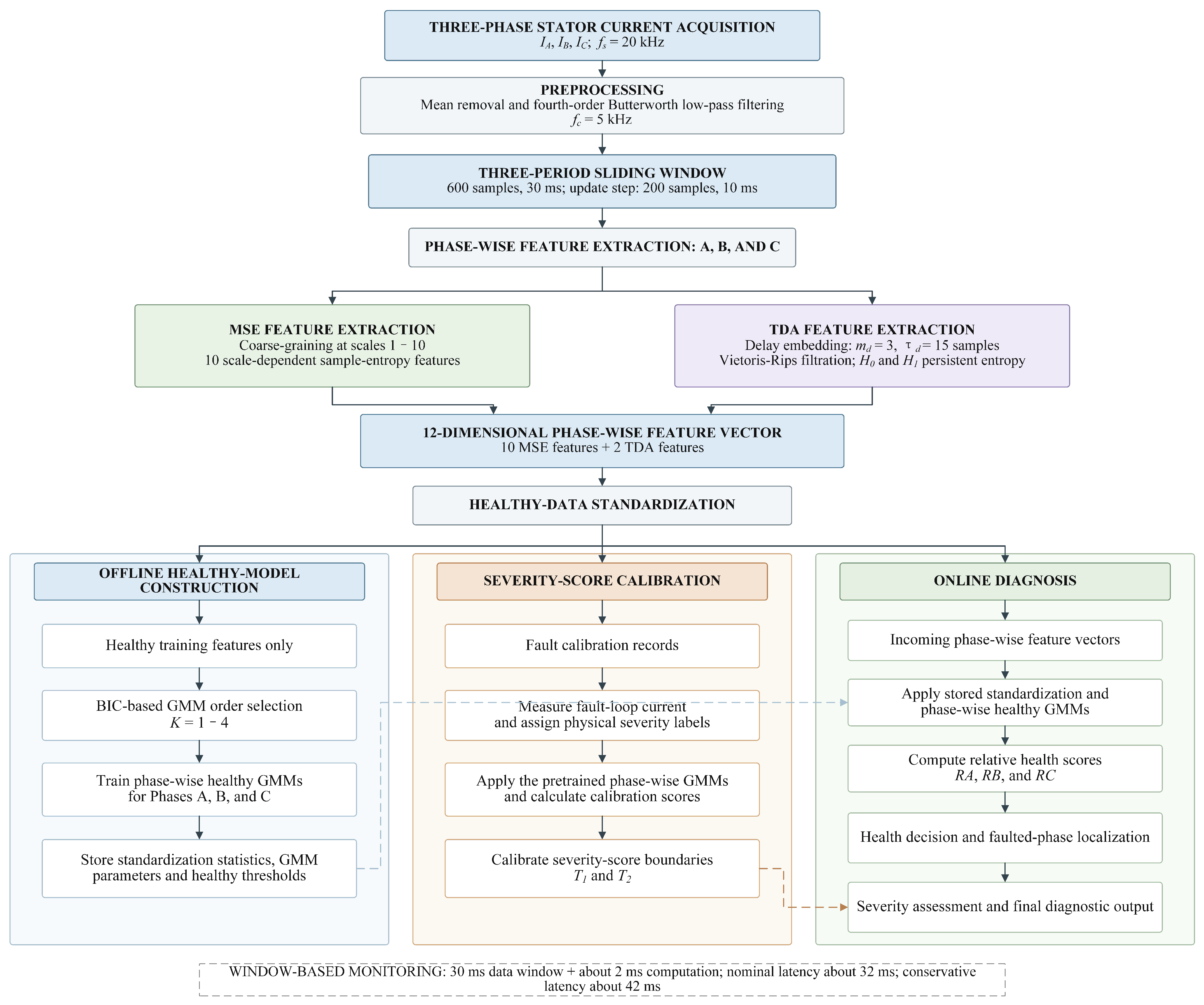
This section describes the complete signal-processing and decision procedure used in the experiments. Each phase-current window is processed by two parallel branches. Multiscale sample entropy (MSE) characterizes scale-dependent waveform irregularity, whereas topological data analysis (TDA) characterizes the delay-coordinate point cloud through persistent homology. Ten MSE components and two persistent-entropy components form a 12-dimensional phase-wise feature vector. A separate Gaussian mixture model (GMM) is fitted to the healthy features of each phase. During operation, the three phase-wise likelihoods are used to detect an abnormal condition, identify the phase with the largest departure from its healthy distribution, and assign a severity level.

Figure 2 summarizes offline model construction, severity-score calibration, and online diagnosis. Training and test data are subjected to the same windowing, preprocessing, feature extraction, and standardization steps.

3.1. Current Preprocessing and Diagnostic Window Construction

For phase $\varphi \in \{A,B,C\}$, the raw sampled current in a buffered acquisition record is denoted by $i_{\varphi ,0}\left(k\right)$. Its DC component is removed by mean subtraction:

$$i_{\varphi ,1}\left(k\right)=i_{\varphi ,0}\left(k\right)-{\overline{i}}_{\varphi ,0},$$

(48)

where ${\overline{i}}_{\varphi ,0}$ is the mean of the buffered record.

A fourth-order Butterworth low-pass filter with a cutoff frequency of $5\mathrm{kHz}$ is subsequently applied to suppress the dominant PWM ripple and high-frequency measurement noise while retaining the fundamental current and the low-order distortion associated with an ISCF. Zero-phase filtering is implemented in MATLAB R2023a using filtfilt on the buffered current record. The filtered sequence, denoted by $i_{\varphi }\left(k\right)$, is then used to identify the electrical-period boundaries and construct the diagnostic windows. This order corresponds to the processing sequence shown in Figure 2: filtering reduces high-frequency ripple and noise before positive-going zero crossings are used for period alignment.

The tested motor has four pole pairs and operates at a rated speed of $1500\mathrm{r}/\min$, corresponding to an electrical frequency of $f_e=100\mathrm{Hz}$. With a sampling frequency of $f_s=20\mathrm{kHz}$, one electrical period contains

$$N_s={\displaystyle \frac{f_s}{f_e}}={\displaystyle \frac{20000}{100}}=200$$

(49)

samples. Positive-going zero crossings are used to locate the period boundaries. Three consecutive electrical periods are concatenated to form one diagnostic window:

$$N=3N_s=600.$$

(50)

The acquisition time of one window is therefore $30\mathrm{ms}$. Adjacent windows are shifted by one electrical period, giving a score update interval of $10\mathrm{ms}$. The same 600-sample window is used for healthy-model construction and for diagnosis. The three-period current traces correspond to the complete diagnostic window defined in Equation (50).

Filtering and period segmentation have distinct roles and are applied in the order shown in Figure 2. Filtering first attenuates high-frequency interference in the sampled current sequence, thereby improving the stability of the subsequent positive-going zero-crossing detection. Period segmentation then synchronizes the filtered samples to the fundamental electrical period and produces fixed-length windows with comparable phase coverage. This synchronization prevents changes in record length or starting phase from being interpreted as changes in MSE or point-cloud topology. The term period therefore refers throughout this paper to the fundamental electrical-current period, not to the PWM carrier period.

When the electrical frequency varies, the period length is updated as

$$N_s\left(k\right)=\mathrm{round}\left({\displaystyle \frac{f_s}{\widehat{f_e}\left(k\right)}}\right),$$

(51)

where $\widehat{f_e}\left(k\right)$ is estimated from adjacent positive-going zero crossings.

3.2. Multiscale Sample-Entropy Feature Extraction

Sample entropy estimates the probability that two signal patterns that are similar for $m_s$ consecutive samples remain similar when their length is increased to $m_s+1$ [20]. Multiscale entropy evaluates this quantity after the signal has been coarse-grained at several temporal scales [21]. In the present method, the individual scale-dependent sample-entropy values, rather than their average, are retained as diagnostic features.

For one preprocessed current window

$${\mathit{i}}_{\varphi }=\{i_{\varphi }\left(1\right),i_{\varphi }\left(2\right),\dots ,i_{\varphi }\left(N\right)\},$$

(52)

the coarse-grained sequence at scale $\tau$ is

$$y_{\varphi ,j}^{\left(\tau \right)}={\displaystyle \frac{1}{\tau }}{\displaystyle \sum _{t=(j-1)\tau +1}^{j\tau }}{i}_{\varphi }\left(t\right),j=1,2,\dots ,N_{\tau },$$

(53)

where

$$N_{\tau }=⌊{\displaystyle \frac{N}{\tau }}⌋.$$

(54)

Small values of $\tau$ preserve local waveform fluctuations, whereas larger values represent the signal over longer temporal scales.

For each scale, the $m_s$-dimensional template vector is

$${\mathit{u}}_{\varphi ,j}^{(m_s,\tau )}=\left[y_{\varphi ,j}^{\left(\tau \right)},y_{\varphi ,j+1}^{\left(\tau \right)},\dots ,y_{\varphi ,j+m_s-1}^{\left(\tau \right)}\right].$$

(55)

The distance between two templates is evaluated using the Chebyshev metric:

$$d_{j,l}^{(m_s,\tau )}=\underset{0\le q<m_s}{\max }\left|y_{\varphi ,j+q}^{\left(\tau \right)}-y_{\varphi ,l+q}^{\left(\tau \right)}\right|.$$

(56)

Self-matches are excluded. Let $B_{\varphi }^{(m_s,\tau )}$ be the normalized number of template pairs satisfying $d_{j,l}^{(m_s,\tau )}\le r$, and let $A_{\varphi }^{(m_s+1,\tau )}$ be the corresponding normalized number for templates of dimension $m_s+1$. The sample entropy at scale $\tau$ is

$$S{E}_{\varphi }^{\left(\tau \right)}=-\ln \left({\displaystyle \frac{A_{\varphi }^{(m_s+1,\tau )}+{ϵ}_{SE}}{B_{\varphi }^{(m_s,\tau )}+{ϵ}_{SE}}}\right),$$

(57)

where ${ϵ}_{SE}={10}^{-12}$ prevents numerical singularity.

The parameters are fixed at

$$m_s=2,r=0.2{\sigma }_{\varphi },\tau =1,2,\dots ,10,$$

(58)

where ${\sigma }_{\varphi }$ is the standard deviation of the original 600-sample window. The choice $m_s=2$ limits the number of samples required for reliable pattern matching, while $r=0.2{\sigma }_{\varphi }$ provides a compromise between noise sensitivity and excessive pattern matching. The scale factor is a positive integer, $\tau \in {\mathbb{N}}^{+}$, and its relation to the window length is given by $N_{\tau }=\lfloor N/\tau \rfloor$. A valid scale must satisfy $N_{\tau }\ge m_s+1$. The selected range $\tau =1,\dots ,10$ satisfies this condition with a substantial margin for $N=600$. The maximum retained scale is 10; consequently, the coarsest sequence still contains 60 samples, which is sufficient for the selected template dimension.

The MSE feature vector is therefore

$${\mathit{f}}_{\varphi ,\mathrm{MSE}}={\left[S{E}_{\varphi }^{\left(1\right)},S{E}_{\varphi }^{\left(2\right)},\dots ,S{E}_{\varphi }^{\left(10\right)}\right]}^{\mathrm{T}}.$$

(59)

The scale-dependent values are retained separately because their variation with $\tau$ is part of the diagnostic information.

3.3. Topological Feature Extraction from the Reconstructed Current Trajectory

3.3.1. Delay-Coordinate Reconstruction

Delay-coordinate embedding provides the theoretical basis for representing a scalar observation by a sequence of delayed coordinates [22]. In this study, the theorem is used to motivate a consistent geometric representation of the measured current; it is not used to claim that a finite, noisy window exactly reconstructs the complete PMSM state space. The unsupported statement that the attractor dimension of the PMSM is smaller than two is therefore not required.

For phase $\varphi$, the reconstructed state vector is

$${\mathit{z}}_{\varphi ,k}={\left[i_{\varphi }\left(k\right),i_{\varphi }(k+{\tau }_d),\dots ,i_{\varphi }(k+(m_d-1){\tau }_d)\right]}^{\mathrm{T}},$$

(60)

where

$$k=1,2,\dots ,N_p,N_p=N-(m_d-1){\tau }_d.$$

(61)

The embedding parameters are fixed at

$$m_d=3,{\tau }_d=15.$$

(62)

At $20\mathrm{kHz}$, a delay of 15 samples corresponds to $0.75\mathrm{ms}$, or 7.5% of one rated electrical period. This value separates the delayed coordinates sufficiently to avoid an almost diagonal point cloud while preserving their short-term dependence. A three-dimensional representation is the lowest-dimensional embedding used here to describe a closed periodic trajectory without relying on a single two-coordinate projection. For $N=600$, the reconstructed point cloud contains

$$N_p=600-2\times 15=570$$

(63)

points in ${\mathbb{R}}^3$.

Under healthy operation, the reconstructed points are concentrated around a repeatable closed trajectory. An ISCF changes the waveform and consequently modifies the local density, dispersion, and loop structure of the point cloud.

This representation is not a Park- or Clarke-vector current hodograph. Park-vector diagnostic curves are constructed by jointly transforming simultaneous three-phase currents [23], whereas ${\mathcal{Z}}_{\varphi }$ is constructed independently from delayed samples of one scalar phase current.

3.3.2. Vietoris–Rips Filtration and Persistent Homology

Let

$${\mathcal{Z}}_{\varphi }=\{{\mathit{z}}_{\varphi ,1},\dots ,{\mathit{z}}_{\varphi ,N_p}\}$$

(64)

be the reconstructed point cloud. Euclidean distance is used to measure the separation between two points. For a filtration parameter $\epsilon$, the Vietoris–Rips complex is defined by

$${\mathrm{VR}}_{\epsilon }\left({\mathcal{Z}}_{\varphi }\right)=\left\{\sigma \subseteq {\mathcal{Z}}_{\varphi }:{\parallel {\mathit{z}}_p-{\mathit{z}}_q\parallel }_2\le \epsilon ,\forall {\mathit{z}}_p,{\mathit{z}}_q\in \sigma \right\}.$$

(65)

Here, $\epsilon$ is the proximity parameter, i.e., the Euclidean-distance threshold used to connect reconstructed points. It is not a single tuned diagnostic feature. The persistence routine evaluates the sequence of finite birth and death values implied by the pairwise Euclidean distances in each reconstructed point cloud. As $\epsilon$ increases, the complexes form a nested filtration. Persistent homology records the values of $\epsilon$ at which topological structures appear and disappear [24,25]. The calculation uses coefficients in ${\mathbb{Z}}_2$ and retains the two homology groups relevant to the measured current trajectory:

• $H_0$, representing connected components of the reconstructed point cloud;
• $H_1$, representing one-dimensional closed loops associated with the periodic trajectory.

All $H_0$ components are born at $\epsilon =0$ and merge as the filtration parameter increases. If the persistence routine returns an essential $H_0$ interval with an infinite death value, this interval is removed before entropy calculation. The finite persistence pairs are denoted by

$${\mathcal{P}}_q={\left\{(b_{q,i},d_{q,i})\right\}}_{i=1}^{n_q},q\in \{0,1\},$$

(66)

where $b_{q,i}$ and $d_{q,i}$ are the birth and death values of the ith structure. Its lifetime is

$$L_{q,i}=\max (0,d_{q,i}-b_{q,i}).$$

(67)

The detailed results will be presented and discussed in the next section.

3.3.3. Persistent-Entropy Features and Experimental Interpretation

Persistent entropy summarizes the distribution of persistence lifetimes in a single scalar [26]. Consistent with the MATLAB implementation, lifetimes smaller than ${10}^{-6}$ are replaced by ${10}^{-6}$. For homology order q, the total lifetime and normalized weights are

$$L_{q,\mathrm{total}}={\displaystyle \sum _{i=1}^{n_q}}{L}_{q,i},p_{q,i}={\displaystyle \frac{L_{q,i}}{L_{q,\mathrm{total}}}}.$$

(68)

The weights are lower-bounded by ${10}^{-12}$, and the persistent entropy is

$$P{E}_{\varphi ,H_q}=-{\displaystyle \sum _{i=1}^{n_q}}{p}_{q,i}\ln p_{q,i},q\in \{0,1\}.$$

(69)

If no finite interval is available for one homology order, the corresponding persistent entropy is set to zero.

The MATLAB implementation also calculates $P{E}_{\varphi ,H_0}+P{E}_{\varphi ,H_1}$ as a topological-complexity index. This sum is not used as an additional GMM input because it is an exact linear combination of the two persistent-entropy components and therefore contains no independent information. The TDA feature vector is

$${\mathit{f}}_{\varphi ,\mathrm{TDA}}={\left[P{E}_{\varphi ,H_0},P{E}_{\varphi ,H_1}\right]}^{\mathrm{T}}.$$

(70)

3.4. Feature Fusion and Healthy-Data Standardization

A diagnostic feature is defined here as a scalar descriptor calculated from one finite phase-current window. It characterizes one property of the signal but does not, by itself, constitute a fault decision. The complete feature vector is the input to the statistical model, whereas the GMM likelihood and relative health score are decision variables.

For each phase, the ten MSE components and two TDA components are concatenated to form

$${\mathit{F}}_{\varphi }={\left[S{E}_{\varphi }^{\left(1\right)},\dots ,S{E}_{\varphi }^{\left(10\right)},P{E}_{\varphi ,H_0},P{E}_{\varphi ,H_1}\right]}^{\mathrm{T}}\in {\mathbb{R}}^{12}.$$

(71)

The first ten components describe waveform irregularity over increasing temporal scales. The 11th component characterizes the distribution of connected-component lifetimes, and the 12th component characterizes the distribution of loop lifetimes.

Because the numerical ranges of the 12 components are different, the features are standardized before GMM training. For feature index d,

$${\tilde{F}}_{\varphi ,d}={\displaystyle \frac{F_{\varphi ,d}-{\mu }_{\varphi ,d}^{\mathrm{H}}}{{\sigma }_{\varphi ,d}^{\mathrm{H}}+{ϵ}_z}},d=1,\dots ,12,$$

(72)

where ${\mu }_{\varphi ,d}^{\mathrm{H}}$ and ${\sigma }_{\varphi ,d}^{\mathrm{H}}$ are calculated exclusively from the healthy training data and ${ϵ}_z={10}^{-12}$. The same stored statistics are applied to all subsequent test samples.

3.5. Phase-Wise Healthy-Distribution Modeling and Diagnosis

3.5.1. GMM Configuration and Healthy-Data Training

Independent healthy models are constructed for Phases A, B, and C to account for small inherent differences among the measured phase currents. For phase $\varphi$, the density of the standardized healthy feature vector is represented by

$$p_{\varphi }\left({\tilde{\mathit{F}}}_{\varphi }\mid {\Theta }_{\varphi }\right)={\displaystyle \sum _{k=1}^{K_{\varphi }}}{\pi }_{\varphi ,k}\mathcal{N}\left({\tilde{\mathit{F}}}_{\varphi };{\mathit{\mu }}_{\varphi ,k},{\mathbf{\Sigma }}_{\varphi ,k}\right),$$

(73)

where ${\pi }_{\varphi ,k}$, ${\mathit{\mu }}_{\varphi ,k}$, and ${\mathbf{\Sigma }}_{\varphi ,k}$ are the mixture weight, mean vector, and covariance matrix of component k, respectively. The parameters are estimated from healthy samples using the expectation–maximization algorithm [27].

The MATLAB implementation uses the following configuration:

• candidate component numbers $K_{\varphi }\in \{1,2,3,4\}$;
• phase-specific model order selected by the minimum Bayesian information criterion (BIC) [28];
• diagonal, non-shared covariance matrices;
• covariance regularization of ${10}^{-6}$;
• k-means++ initialization;
• 20 independent EM replicates;
• maximum 1000 iterations and convergence tolerance ${10}^{-6}$;
• random seed 2026.

The candidate range of one to four components allows modest flexibility in representing possible multimodality among the independently acquired healthy datasets without imposing four components on every phase. BIC penalizes unnecessary components and selects the model order separately for each phase. Diagonal covariance matrices reduce the number of parameters relative to unrestricted full covariance matrices and improve numerical stability for a 12-dimensional input with a limited number of independent healthy acquisition records.

3.5.2. Relative Health Score, Fault Localization, and Severity Assessment

For a test feature vector, the phase-wise log-likelihood is

$${\mathsf{\ell }}_{\varphi }=\ln p_{\varphi }\left({\tilde{\mathbf{F}}}_{\varphi }\mid {\Theta }_{\varphi }\right).$$

(74)

A lower log-likelihood indicates a larger deviation from the healthy feature distribution. To obtain a positive index whose healthy values are centered near one and which decreases as the deviation increases, the relative health score is defined as

$$R_{\varphi }=\exp \left[{\displaystyle \frac{{\mathsf{\ell }}_{\varphi }-{\tilde{\mathsf{\ell }}}_{\varphi }^{\mathrm{H}}}{3\mathrm{IQR}\left({\mathsf{\ell }}_{\varphi }^{\mathrm{H}}\right)+{ϵ}_R}}\right],$$

(75)

where ${\tilde{\mathsf{\ell }}}_{\varphi }^{\mathrm{H}}$ and $\mathrm{IQR}\left({\mathsf{\ell }}_{\varphi }^{\mathrm{H}}\right)$ are the median and interquartile range of healthy reference log-likelihoods, and ${ϵ}_R={10}^{-12}$. This monotonic normalization preserves the ordering given by the original GMM likelihood. The phase-wise scores are combined through the minimum-score index $R_{{\varphi }^{*}}={\min }_{\varphi \in \{A,B,C\}}{R}_{\varphi }$.

The healthy threshold for phase $\varphi$ is determined from the lower tail of its healthy reference scores:

$$T_{\varphi }^{\mathrm{H}}=Q_{0.01}\left(R_{\varphi }^{\mathrm{H}}\right),$$

(76)

where $Q_{0.01}$ denotes the first percentile. The motor is classified as healthy only when

$$R_A\ge T_A^{\mathrm{H}},R_B\ge T_B^{\mathrm{H}},R_C\ge T_C^{\mathrm{H}}.$$

(77)

For every test window, the phase with the minimum relative health score is defined as

$${\varphi }^{*}=\arg \underset{\varphi \in \{A,B,C\}}{\min }{R}_{\varphi }.$$

(78)

If all three phase-wise scores satisfy Equation (77), the motor is classified as healthy and ${\varphi }^{*}$ is used only to define the minimum score reported for visualization. If at least one phase violates its healthy threshold, ${\varphi }^{*}$ identifies the faulted phase. This rule is consistent with the analytical result in Section 2, according to which the current perturbation of the directly faulted phase is larger than the perturbations of the other two phases.

Only healthy samples are used to estimate the GMM parameters. However, the terms mild, moderate, and severe have a physical meaning defined by the measured short-circuit-current amplitude. Accordingly, the mapping from the one-dimensional health score to these three severity levels is calibrated once using the short-circuit-current groups defined in the experimental section; these fault samples are not used to fit the GMM density. Let ${\tilde{R}}_{\mathrm{mild}}$, ${\tilde{R}}_{\mathrm{moderate}}$, and ${\tilde{R}}_{\mathrm{severe}}$ be the median scores of the faulted phase for the three severity groups. The internal severity boundaries are

$$T_1={\displaystyle \frac{{\tilde{R}}_{\mathrm{mild}}+{\tilde{R}}_{\mathrm{moderate}}}{2}},T_2={\displaystyle \frac{{\tilde{R}}_{\mathrm{moderate}}+{\tilde{R}}_{\mathrm{severe}}}{2}}.$$

(79)

The four-state decision rule is

$$\mathrm{State}=\left\{\begin{array}{cc}\mathrm{Healthy},\hfill & R_{\varphi }\ge T_{\varphi }^{\mathrm{H}}\mathrm{for}\mathrm{all}\mathrm{phases},\hfill \\ \mathrm{Mild}\mathrm{ISCF},\hfill & T_1\le R_{{\varphi }^{*}}<T_{{\varphi }^{*}}^{\mathrm{H}},\hfill \\ \mathrm{Moderate}\mathrm{ISCF},\hfill & T_2\le R_{{\varphi }^{*}}<T_1,\hfill \\ \mathrm{Severe}\mathrm{ISCF},\hfill & R_{{\varphi }^{*}}<T_2.\hfill \end{array}\right.$$

(80)

The GMM density estimation is one-class and uses only healthy data; no fault labels are required for model fitting. The three fault-severity labels are assigned through a separate calibration of the one-dimensional health score and are not represented by additional GMM class densities.

3.6. Computational Complexity and Online Capability

Let N denote the number of samples in one phase-current window, S the number of retained MSE scales, $N_p$ the number of reconstructed points, D the fused-feature dimension, and K the number of Gaussian components. Mean removal and fourth-order filtering require $\mathcal{O}\left(N\right)$ operations. With the direct pairwise implementation of sample entropy, the MSE branch requires

$$\mathcal{O}\left(m_s{\displaystyle \sum _{\tau =1}^S}{⌊{\displaystyle \frac{N}{\tau }}⌋}^2\right)$$

(81)

operations. Since $S=10$ and $m_s=2$ are fixed, this term is quadratic in the window length.

Delay-coordinate reconstruction requires $\mathcal{O}\left(m_d{N}_p\right)$ operations. The pairwise Euclidean-distance calculation used for the Vietoris–Rips filtration requires $\mathcal{O}\left(m_d{N}_p^2\right)$ operations and $\mathcal{O}\left(N_p^2\right)$ memory. Persistent-homology reduction has data-dependent cost because the number of simplices increases with point-cloud density and the maximum filtration radius. To limit this cost, only $H_0$ and $H_1$ are retained and the embedding dimension is fixed at three. For the present setting, $N_p=570$, and the dense pairwise-distance matrix contains ${570}^2=324,900$ entries, corresponding to approximately $2.5\mathrm{MB}$ in double precision.

GMM parameter estimation is performed offline. With diagonal covariance matrices, one EM iteration for $n_H$ healthy feature vectors requires $\mathcal{O}\left(n_{H}KD\right)$ operations. Online evaluation of one phase requires $\mathcal{O}\left(KD\right)$ operations, which is negligible compared with MSE and persistent-homology calculation because $D=12$ and $K\le 4$.

The online acquisition and diagnostic calculations were performed on the same desktop computer using MATLAB R2023a under 64-bit Windows 10 Pro, version 22H2. The computer was equipped with a 13th-generation Intel Core i5-13400 processor ($2.50\mathrm{GHz}$) and $16\mathrm{GB}$ of RAM. An NVIDIA GeForce GTX 1650 ($4\mathrm{GB}$) graphics card was installed, but dedicated GPU acceleration is not required by the proposed method; the reported implementation runs in standard MATLAB on the CPU. The approximately $2.5\mathrm{MB}$ dense distance matrix is therefore small relative to the available system memory.

The current window contains three electrical periods and therefore requires $30\mathrm{ms}$ of data acquisition at the rated operating point. On the above platform, after the models have been loaded, the MATLAB implementation requires approximately $2\mathrm{ms}$ per three-phase window for preprocessing, feature extraction, and GMM evaluation, excluding data acquisition and file input/output. The nominal latency is therefore approximately $32\mathrm{ms}$. Since windows are updated every electrical period, a fully post-fault window is available within at most $40\mathrm{ms}$ after fault inception, giving a conservative latency of approximately $42\mathrm{ms}$ including computation. The use of filtfilt makes the implementation window-based rather than sample-causal; the method is therefore intended for online condition monitoring and early warning, not for instantaneous protective tripping.

3.7. Implementation Parameters and Complete Procedure

Table 1. Implementation parameters of the proposed MSE–TDA–GMM method.

Module	Parameter	Value
Sampling	Sampling frequency	$20\mathrm{kHz}$
Segmentation	Samples per period	200
Segmentation	Diagnostic window	3 periods, 600 samples
Segmentation	Sliding step	1 period, 200 samples
Filtering	Butterworth order/cutoff	4/$5\mathrm{kHz}$
MSE	Template dimension	$m_s=2$
MSE	Matching tolerance	$r=0.2{\sigma }_{\varphi }$
MSE	Retained scales	1–10
TDA	Embedding dimension	$m_d=3$
TDA	Time delay	${\tau }_d=15$ samples
TDA	Point-cloud size	570 points
TDA	Distance/homology	Euclidean/$H_0,H_1$
TDA	Lifetime lower bound	${10}^{-6}$
TDA	Probability lower bound	${10}^{-12}$
GMM	Candidate components	$K=1$–4, selected by BIC
GMM	Covariance	diagonal, non-shared
GMM	Regularization	${10}^{-6}$
GMM	EM settings	20 replicates, 1000 iterations, tolerance ${10}^{-6}$
Execution	Software/operating system	MATLAB R2023a/Windows 10 Pro 22H2 (64-bit)
Execution	Processor/memory	Intel Core i5-13400 ($2.50\mathrm{GHz}$)/$16\mathrm{GB}$ RAM
Execution	Dedicated GPU requirement	None

summarizes the parameters used in the complete method.

The offline procedure is as follows: (1) apply mean removal and low-pass filtering to the acquired current records; (2) identify the electrical-period boundaries and construct three-period windows; (3) calculate the ten MSE components and two TDA components for each phase; (4) standardize the 12-dimensional vectors using healthy training statistics; (5) select the GMM order by BIC and estimate one model for each phase; and (6) store the standardization parameters, GMM parameters, healthy thresholds, and severity boundaries.

During diagnosis, each incoming window is processed using the same feature-extraction and standardization chain. The three relative health scores are then calculated from the pretrained phase-wise GMMs. Equations (77), (78) and (80) provide the health decision, faulted-phase localization, and severity classification, respectively.

4. Experimental Verification

4.1. Test Motor, Fault Emulator, and Data Acquisition

An 8-pole, 12-slot PMSM rated at $1.5\mathrm{kW}$ was used as the experimental prototype. Its principal parameters are listed in

Table 2. Main parameters of the tested permanent magnet synchronous motor.

Specification	Symbol	Value	Unit
Rated Power	$P_r$	1.5	kW
Rated Speed	$n_b$	1500	rpm
Rated Voltage	U	220	V
Rated Current	$I_r$	4.4	A
Rated Torque	$T_e$	9.5	N·m
Pole Pairs	p	4	—
Stator Outer Diameter	$D_{a1}$	120	mm
Stator Inner Diameter	$D_{a2}$	70	mm
Rotor Outer Diameter	$D_{b1}$	68.4	mm
Rotor Inner Diameter	$D_{b2}$	25	mm
Permanent Magnet Radial Thickness	h	5	mm
Air Gap	g	0.8	mm
Phase Resistance	$R_s$	1.5	$\Omega$
Phase Inductance	$L_s$	0.8	mH

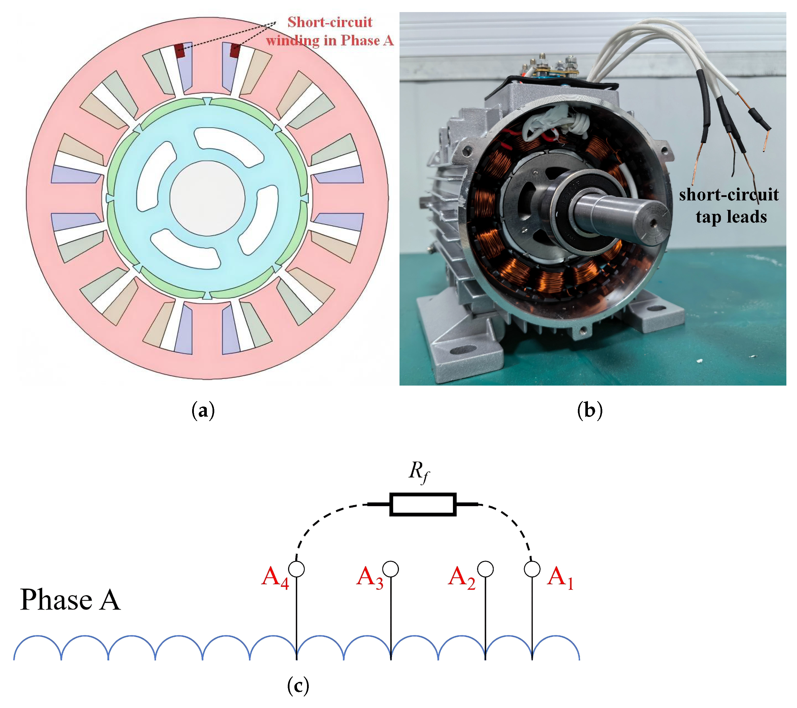
. Figure 3 shows the cross section, physical prototype, and Phase-A tap arrangement.

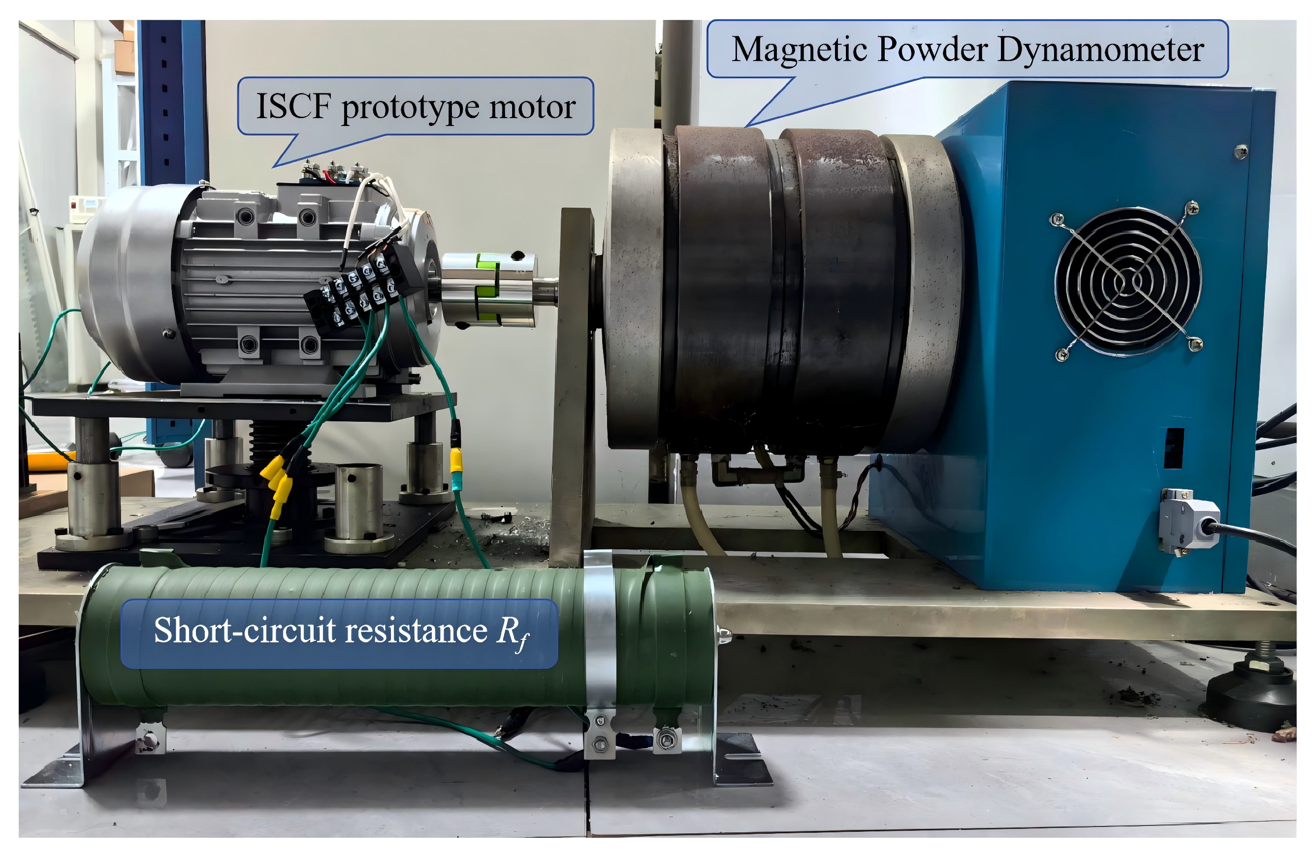
Four tap leads, denoted by $A_1$–$A_4$, were brought out from the Phase-A winding. Tap $A_1$ was used as the common terminal, while the combinations $A_1$–$A_2$, $A_1$–$A_3$, and $A_1$–$A_4$ produced fault sections containing 1, 3, and 5 shorted turns, respectively. An external resistance $R_f$ with a maximum value of $1\Omega$ was connected across the selected taps. The taps remained open during healthy operation. A Hall current probe and oscilloscope measured the fault-loop current, and a magnetic-powder dynamometer provided the mechanical load and measured torque and speed. The experimental test bench is shown in Figure 4.

The laboratory inverter was operated with PWM vector control and a fixed carrier frequency of $8\mathrm{kHz}$. This value is reported as an experimental drive condition; it is neither an optimized semiconductor-loss design choice nor a parameter required by the proposed diagnostic method. The diagnostic algorithm uses the measured stator currents after the $5\mathrm{kHz}$ low-pass filtering described in Section 3.1, so the carrier-related ripple is treated as interference rather than as a fault feature. Semiconductor junction-temperature and switching-loss characterization were outside the scope of this study.

The three-phase currents were sampled at $20\mathrm{kHz}$. Each retained diagnostic sample consisted of one three-period, 600-sample current window as defined in Equation (50). The acquired records were partitioned at the record level into healthy-model training, severity-boundary calibration, and independent testing subsets; windows originating from the same acquisition record were never assigned to different subsets. The same preprocessing, period segmentation, and feature-extraction procedures were applied to all subsets. The final independent test set contained 200 healthy windows and 400 windows for each of the mild, moderate, and severe ISCF states, yielding 1400 test windows in total.

4.2. Healthy-Current Representation and Interpretation

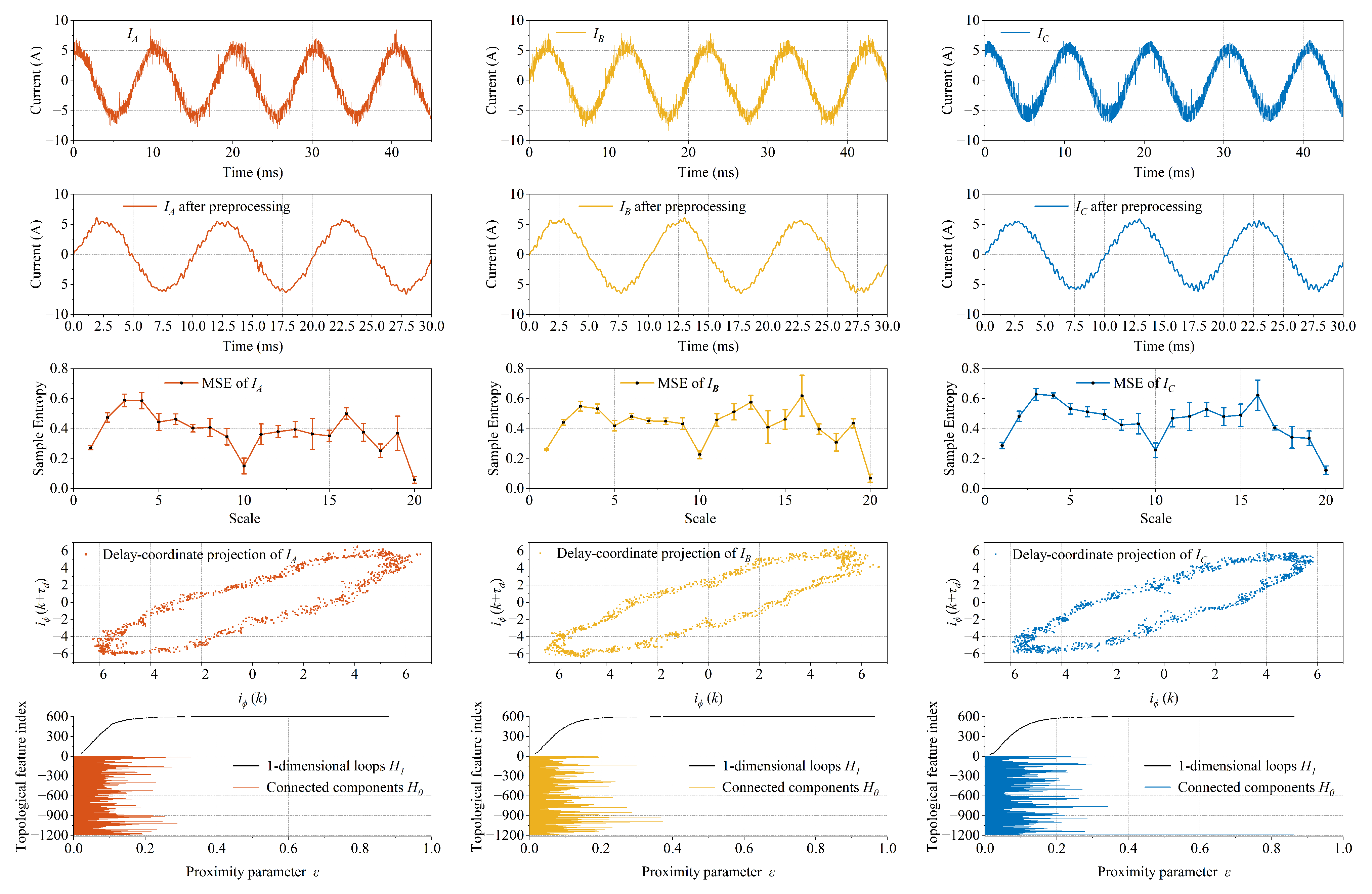
Independent healthy models were constructed for Phases A, B, and C to account for small inherent differences among the measured phase currents. Figure 5 links the processing stages in Section 3 to representative healthy-current data at the rated operating point.

The first row of Figure 5 shows representative raw records. The second row shows filtered and period-aligned waveforms. Filtering and segmentation are distinct operations: the low-pass filter attenuates PWM-related ripple and high-frequency measurement noise before period segmentation aligns the filtered data to the fundamental electrical period and provides fixed-length windows with the same phase coverage. This alignment is important because MSE and TDA are sensitive to the number of samples and to the portion of the periodic trajectory included in a window. Three electrical periods are plotted in the second row, consistent with the three-period, 600-sample windows specified in Equation (50).

The third row presents the scale-dependent sample entropy over scales 1–20 for visualization. The error bars span the minimum-to-maximum range across repeated healthy-current records. Scales 1–10 show stable healthy values while retaining local waveform information; these ten values form the MSE part of the diagnostic vector. Larger scales are not retained because the coarse-grained sequence becomes shorter and local fault-induced changes are increasingly averaged.

The fourth row shows a two-dimensional projection of the three-dimensional delay-coordinate point cloud. The horizontal coordinate is $i_{\varphi }\left(k\right)$ and the vertical coordinate is $i_{\varphi }(k+{\tau }_d)$; the omitted third coordinate is $i_{\varphi }(k+2{\tau }_d)$. The plots therefore describe the geometric relation among delayed samples of a single phase current. They are not obtained from an $abc$-to-$\alpha \beta$ or $abc$-to-$dq$ conversion. Under healthy operation, the points remain concentrated around a repeatable closed trajectory. Changes in waveform shape alter the density, dispersion, and loop structure of this point cloud.

The fifth row shows the persistence intervals generated by the Vietoris–Rips filtration. The horizontal variable $\epsilon$ is the Euclidean-distance threshold used to connect points in the reconstructed space. At $\epsilon =0$, every sampled point is born as an individual $H_0$ connected component. These components merge as $\epsilon$ increases. The $H_1$ intervals record the birth and disappearance of one-dimensional loops. Long intervals represent structures that persist over a wider range of proximity thresholds, whereas short intervals are more sensitive to local perturbations and measurement noise. The lifetime distributions are summarized by $P{E}_{\varphi ,H_0}$ and $P{E}_{\varphi ,H_1}$, which become components 11 and 12 of the fused feature vector.

4.3. Fault-Severity Labels

The measured fault-loop current was used only to define physically interpretable severity labels and to calibrate the score boundaries; it was not used as an input to the GMM. For each fault condition, the fundamental amplitude $|I_{f,1}|$ was extracted from the Hall-probe record and normalized by the rated phase current:

$${\rho }_f={\displaystyle \frac{|I_{f,1}|}{I_r}}.$$

(82)

The three fault levels were defined as

$$\left\{\begin{array}{cc}\mathrm{Mild}\mathrm{ISCF},\hfill & {\rho }_f<1,\hfill \\ \mathrm{Moderate}\mathrm{ISCF},\hfill & 1\le {\rho }_f<1.5,\hfill \\ \mathrm{Severe}\mathrm{ISCF},\hfill & {\rho }_f\ge 1.5.\hfill \end{array}\right.$$

(83)

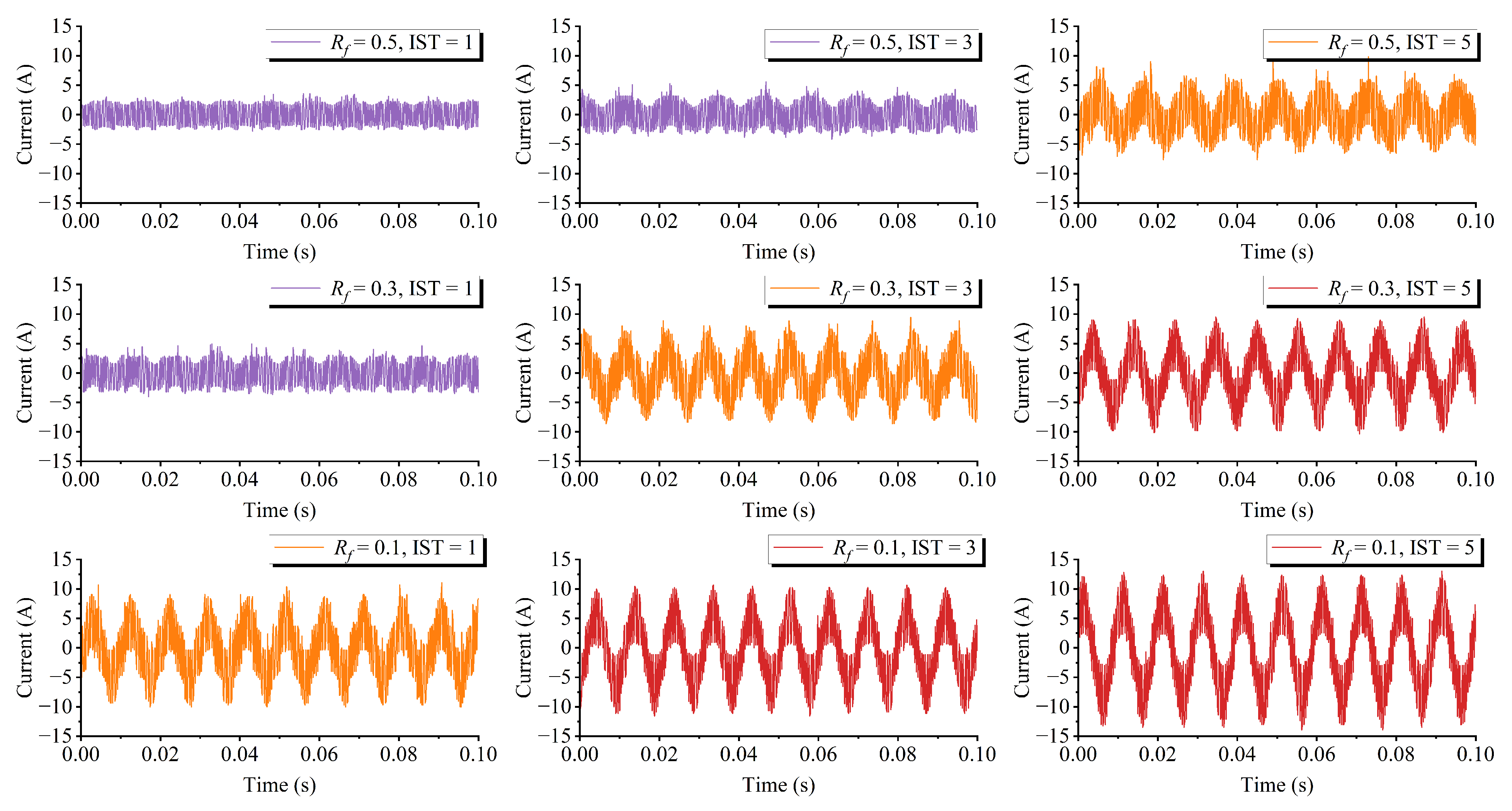
Figure 6 shows the measured fault-loop currents for nine combinations of $R_f$ and the number of shorted turns. Decreasing $R_f$ or increasing the number of shorted turns generally increases the fault-loop current, consistent with Equation (27).

4.4. Experimental Evaluation of the Phase-Wise Diagnostic Features

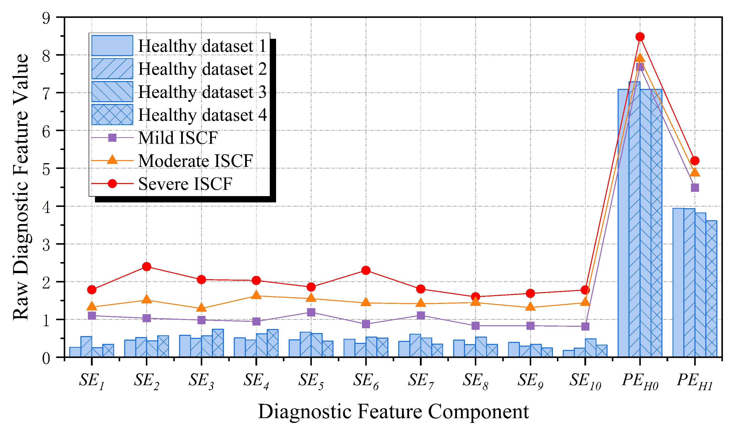
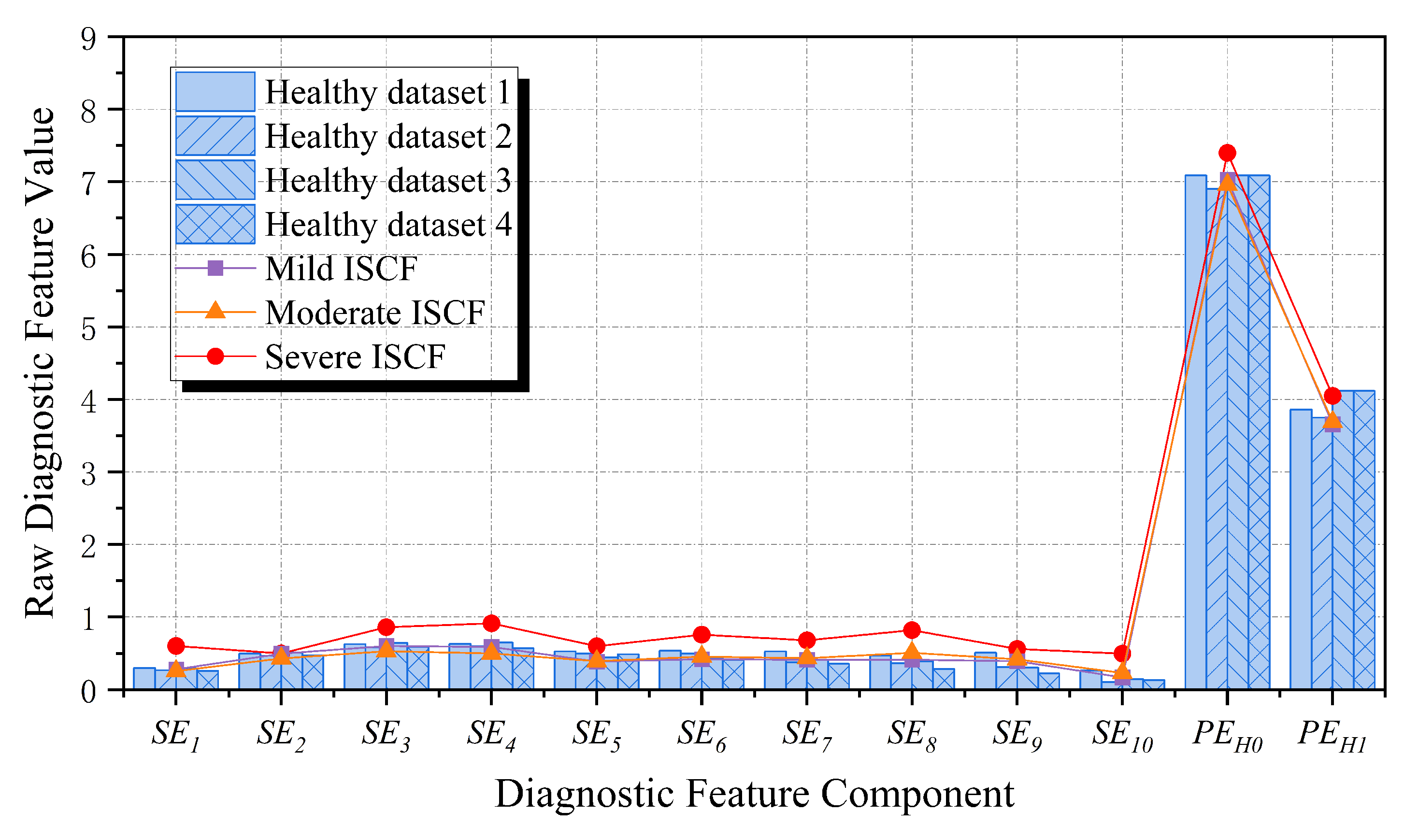
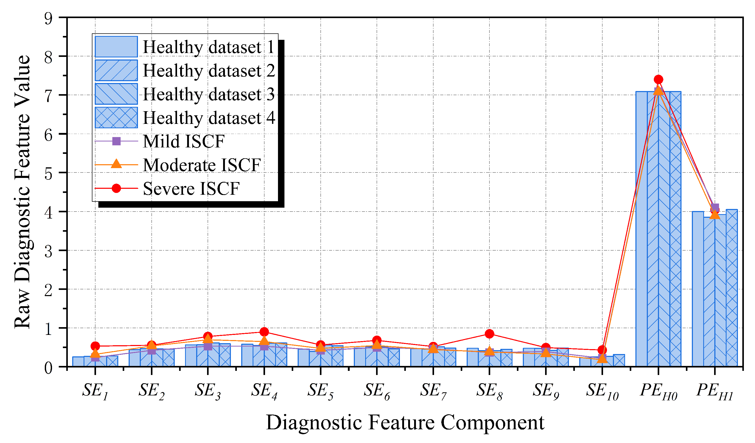
A diagnostic feature is a scalar descriptor extracted from one phase-current window; it is not itself a diagnostic decision. For phase $\varphi$, the complete 12-dimensional feature vector is defined by Equation (71). Components 1–10 are the scale-dependent sample entropies, component 11 is $P{E}_{\varphi ,H_0}$, and component 12 is $P{E}_{\varphi ,H_1}$. All components are dimensionless. Figure 7, Figure 8 and Figure 9 display the raw values to preserve their physical interpretation; standardized values are used internally by the GMM.

The experimental feature behavior is considered from three perspectives. Repeatability is assessed from the dispersion among four independently acquired healthy datasets. Fault sensitivity is assessed from the change in each component as the measured fault-loop-current severity increases. Phase selectivity is assessed by comparing the feature changes of the directly faulted Phase A with those of Phases B and C.

The Phase-A features show the largest departure from their healthy ranges as the fault-loop current increases. The Phase-B and Phase-C features remain closer to their healthy ranges under mild and moderate faults and exhibit smaller changes under the severe condition. This phase-dependent response is consistent with Equation (38), which predicts that the terminal-current perturbation is largest in the directly faulted phase. The three criteria above show how the features are interpreted and evaluated before they are jointly processed by the GMM.

4.5. GMM Health Score and Classification Performance

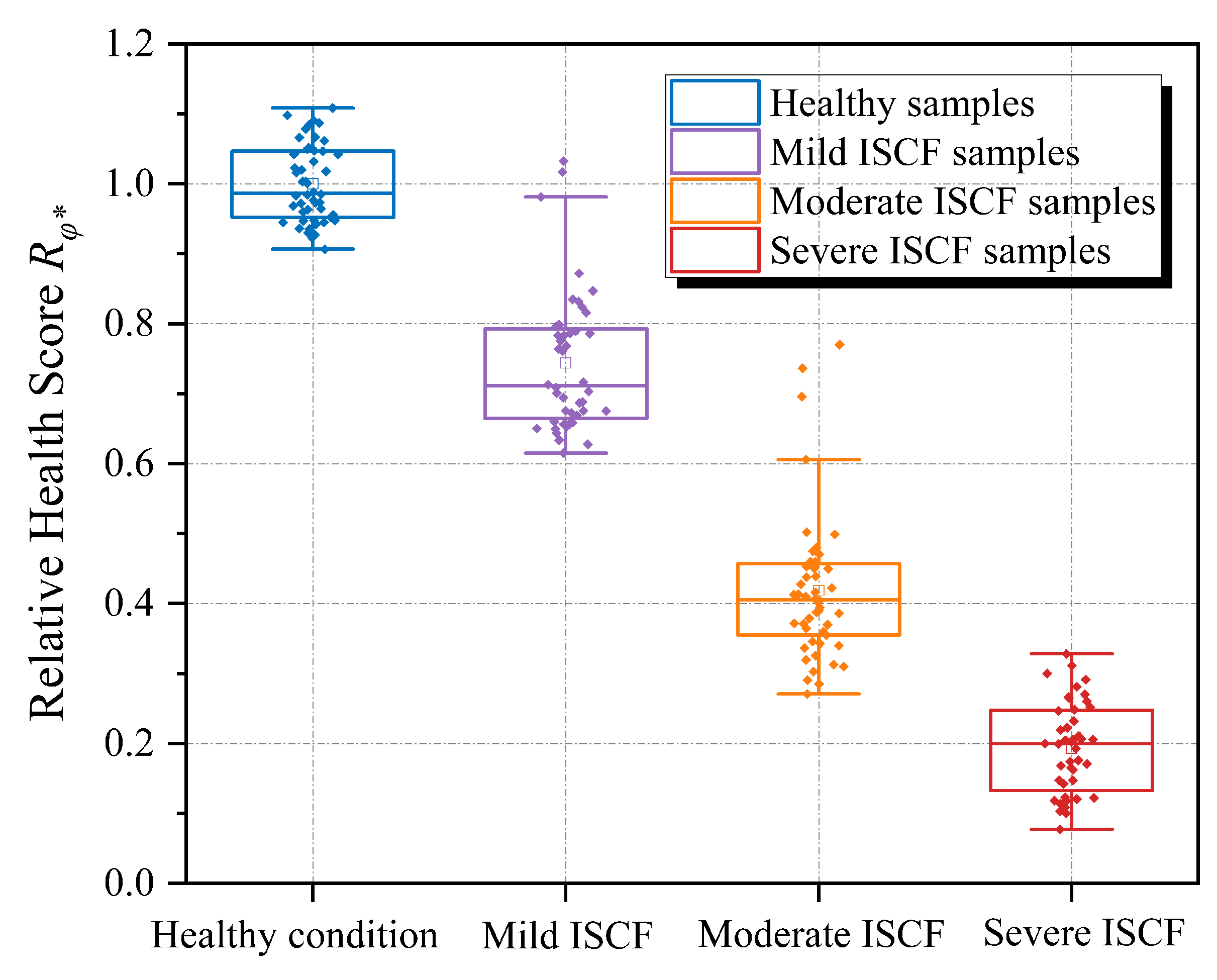
The GMM configuration and decision rules are given in Section 3.5. Figure 10 shows the minimum phase-wise relative health score $R_{{\varphi }^{*}}$. For a detected abnormal condition, ${\varphi }^{*}$ is the identified faulted phase; for a healthy window, it denotes only the phase having the minimum of the three healthy scores. This score is a decision variable derived from the healthy-model likelihood and is not one of the 12 input features.

The healthy scores are concentrated near one. As the fault severity increases, the score distributions progressively shift downward, with partial overlap occurring mainly between adjacent severity levels. The GMM is fitted only to healthy samples. The separation of mild, moderate, and severe faults is produced by the separately calibrated score boundaries in Equation (79); the model does not fit four independent class-conditional GMMs.

Table 3. Classification performance metrics derived from the four-state confusion matrix.

State	Number of Test Samples	Precision (%)	Recall (%)	F1-Score (%)
Healthy	200	98.52	100.00	99.26
Mild ISCF	400	97.49	97.00	97.24
Moderate ISCF	400	96.50	96.50	96.50
Severe ISCF	400	97.99	97.75	97.87
Macro average	—	97.63	97.81	97.72
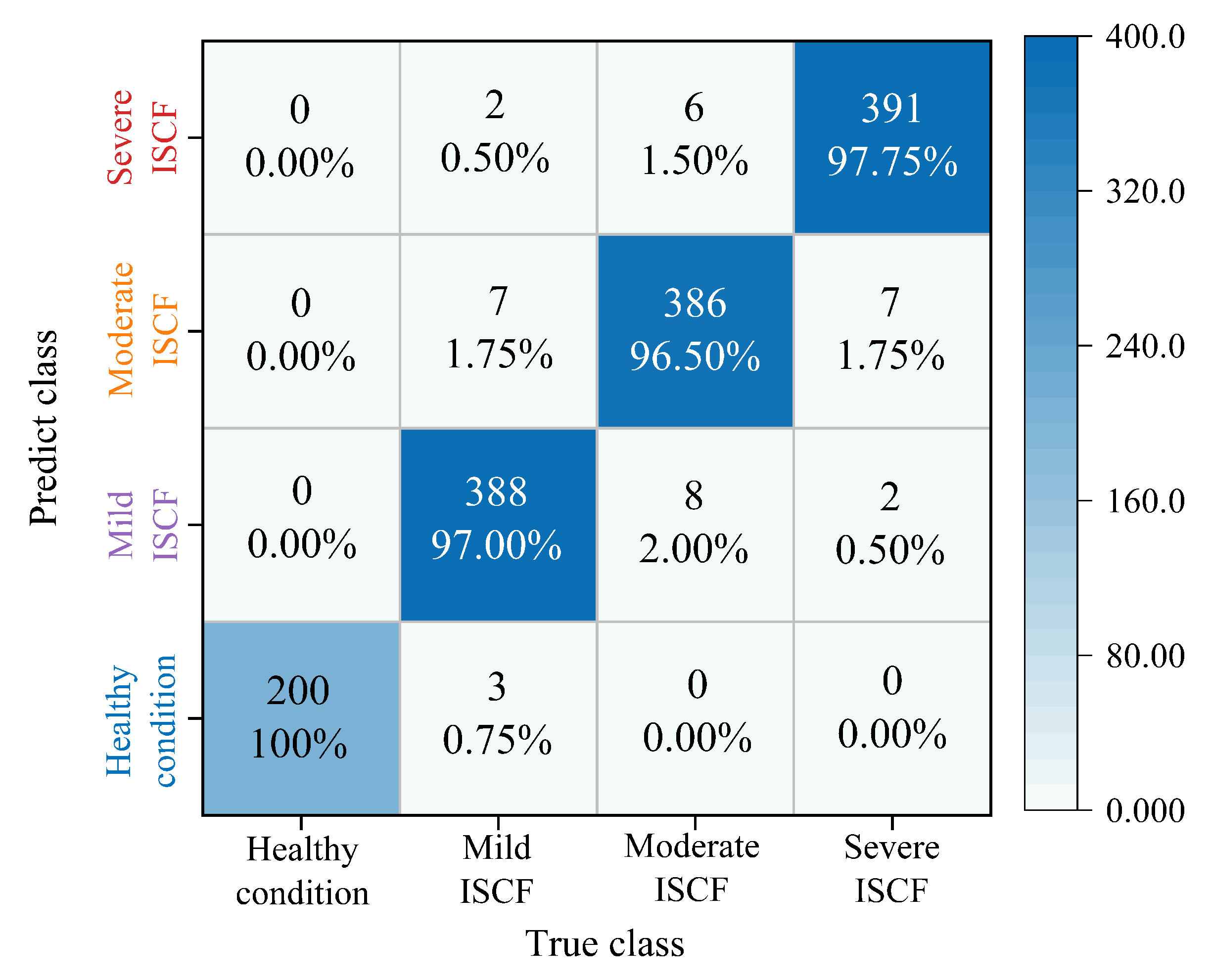
Overall accuracy	1400	97.50%

reports the classification performance metrics derived from the four-state confusion matrix and Figure 11 reports the four-state classification results. The diagonal entries correspond to class-wise recalls of 100% for healthy operation, 97.00% for mild ISCF, 96.50% for moderate ISCF, and 97.75% for severe ISCF. Based on 1365 correct decisions among 1400 test samples, the overall accuracy is 97.50%. The macro-averaged precision, recall, and F1-score are 97.63%, 97.81%, and 97.72%, respectively. Most errors occur between adjacent severity levels, which is consistent with the partial overlap of the score distributions in Figure 10. A small number of mild faults are assigned to the healthy state, indicating that the lowest-severity boundary remains the most demanding decision region.

4.6. Comparison, Practical Scope, and Limitations

Table 4. Quantitative cross-study comparison with representative recent PMSM interturn-fault diagnostic approaches. Reported results were obtained on different datasets and are not an identical-condition benchmark.

Study	Data Basis and Diagnostic Input	Method and Supervision	Reported Quantitative Result
Chen et al. (2024) [15]	Star–delta fractional-slot PM motor; current and torque signals	Optimized VMD and multiscale fuzzy entropy; fault-condition information used to establish diagnostic rules	Classification accuracy above $95\%$
Yan and Hu (2024) [16]	$2.2\mathrm{kW}$ physical PMSM test rig; three-phase current and vibration signals over 10 speed/load combinations; ITSC, demagnetization, and coupled faults	Multiscale residual dilated CNN and BiLSTM; supervised multi-signal learning	Accuracy reported as 4.2% higher than a conventional CNN and 29.06% higher than a BiLSTM
Zsuga and Dineva (2025) [17]	FEM/simulation-derived EV transient dataset; $1\mathrm{s}$, $20\mathrm{kHz}$ current windows represented by DWT coefficients of the Park-vector modulus	Transformer classifier trained with labelled simulated fault data	$97\%$ validation accuracy
Lan et al. (2025) [18]	Simulink–Simplorer–Maxwell joint-simulation data under voltage unbalance; sequence-current components and electromagnetic torque	Multi-task meta-learning with labelled simulated fault tasks	$99.75\pm 0.25\%$ fault-degree accuracy and $99.45\pm 0.21\%$ joint fault-location/degree accuracy
Proposed method	$1.5\mathrm{kW}$ physical PMSM; 1400 independent three-period current windows at the investigated rated operating point	Phase-wise MSE–TDA features and healthy-only GMM density estimation; fault groups used only for severity-boundary calibration	$97.50\%$ overall accuracy and $97.72\%$ macro F1-score

provides a quantitative cross-study comparison with recent entropy-based, deep-learning, and hybrid PMSM interturn-fault diagnostic approaches. Identical-condition retraining was not possible because the cited studies used different motors, fault classes, operating ranges, signals, and data partitions, and the cited studies do not share a common experimental PMSM-ISCF benchmark. The numerical results are therefore quoted as reported by the respective studies and are intended to provide quantitative context rather than a direct ranking.

The reported values show that recent supervised deep-learning and hybrid approaches can achieve high accuracy when labelled fault data or high-fidelity simulation datasets are available. The proposed method achieves an overall accuracy in the same numerical range on physical test-bench data while using only healthy samples to fit the phase-wise density models. Its $30\mathrm{ms}$ diagnostic window is also shorter than the $1\mathrm{s}$ input window reported for the Transformer study. Because the diagnostic tasks and datasets differ, the numerical values should not be interpreted as evidence that one method is universally superior. A same-condition benchmark with shared record-level partitions remains an important direction for future work.

The practical advantages of the proposed method are the use of existing phase-current measurements, the absence of additional injection hardware, and healthy-only density estimation. The phase-wise structure also provides a direct localization rule. The method is nevertheless subject to several limitations. First, the experiments use artificially introduced faults in Phase A of one prototype motor; B- and C-phase faults and naturally developed insulation damage were not tested. Second, the principal results were obtained at the rated operating point. The adaptive period-length calculation supports frequency changes, but broad robustness to speed, load, supply unbalance, and controlled noise levels has not yet been established experimentally. Third, the severity labels require a one-time calibration using measured fault-loop currents. Fourth, the use of filtfilt makes the present MATLAB implementation window-based and noncausal at the sample level. Finally, the GMM thresholds and the distributions of the fused features are machine dependent. These limitations define the scope of the conclusions and motivate cross-machine validation, causal embedded implementation, and same-condition comparisons with conventional and deep-learning baselines.

5. Conclusions

A phase-wise MSE–TDA–GMM framework was developed for incipient interturn short-circuit diagnosis in a PMSM. The analytical model shows that a localized Phase-A fault produces the largest terminal-current perturbation in the directly faulted phase, while the terminal-current change remains weak during the incipient high-resistance stage. This result provides the physical basis for independent phase models and for using descriptors that are sensitive to subtle waveform and dynamical-structure changes.

Each three-period current window is represented by ten scale-dependent sample-entropy components and two persistent-entropy components. The GMM parameters are estimated using healthy data only, and the phase-wise likelihood scores are used for health assessment and phase localization. Severity labels are assigned by separately calibrated score boundaries associated with the measured fault-loop-current groups. Under the investigated experimental conditions, the class-wise recalls range from 96.50% to 100%, with an overall accuracy of 97.50%.

The results support the use of temporal-complexity and topological descriptors as complementary inputs for detecting weak current changes. The present evidence is limited to one prototype motor, artificial Phase-A faults, and principally rated-speed/rated-load operation. Robustness across motors, naturally developed insulation faults, broad speed and load ranges, and controlled noise levels remains to be established. Future work will also investigate causal filtering and embedded persistent-homology implementations, B- and C-phase fault validation, transfer of healthy models between machines, composite faults, and direct comparisons with supervised machine-learning and deep-learning methods under identical data partitions.

References

- Motor Reliability Working Group. Report of Large Motor Reliability Survey of Industrial and Commercial Installations, Part I. IEEE Trans. Ind. Appl. 1985, IA-21, 853–864. [Google Scholar] [CrossRef] [Scilit]
- Jiang, Y.; Ji, B.; Zhang, J.; Yan, J.; Li, W. An Overview of Diagnosis Methods of Stator Winding Interturn Short Faults in Permanent-Magnet Synchronous Motors for Electric Vehicles. World Electr. Veh. J. 2024, 15, 165. [Google Scholar] [CrossRef] [Scilit]
- Obeid, N.H.; Boileau, T.; Nahid-Mobarakeh, B. Modeling and diagnostic of incipient interturn faults for a three phase permanent magnet synchronous motor using wavelet transform. In Proceedings of the 2015 IEEE Industry Applications Society Annual Meeting, Addison, TX, USA, 18–22 October 2015; pp. 1–8. [Google Scholar]
- Romeral, L.; Urresty, J.C.; Riba Ruiz, J.-R.; Garcia Espinosa, A. Modeling of Surface-Mounted Permanent Magnet Synchronous Motors With Stator Winding Interturn Faults. IEEE Trans. Ind. Electron. 2011, 58, 1576–1585. [Google Scholar] [CrossRef] [Scilit]
- Faiz, J.; Nejadi-Koti, H.; Exiri, A.H. Inductance-based Interturn Fault Detection in Permanent Magnet Synchronous Machine Using Magnetic Equivalent Circuit Model. Electr. Power Compon. Syst. 2017, 45, 1016–1030. [Google Scholar] [CrossRef] [Scilit]
- Majma, E.; Setoodeh, P.; Ahmed, R.; Deshpande, U.; Habibi, S. Interturn Short-Circuit Fault Detection and Diagnosis in Permanent Magnet Synchronous Motors Using Interactive Multiple Model Strategy. IEEE Trans. Transp. Electrif. 2026, 12, 2962–2977. [Google Scholar] [CrossRef] [Scilit]
- Qi, Y.; Bostanci, E.; Zafarani, M.; Akin, B. Severity Estimation of Interturn Short Circuit Fault for PMSM. IEEE Trans. Ind. Electron. 2019, 66, 7260–7269. [Google Scholar] [CrossRef] [Scilit]
- Alloui, A.; Laadjal, K.; Sahraoui, M.; Marques Cardoso, A.J. Online Interturn Short-Circuit Fault Diagnosis in Induction Motors Operating Under Unbalanced Supply Voltage and Load Variations, Using the STLSP Technique. IEEE Trans. Ind. Electron. 2023, 70, 3080–3089. [Google Scholar] [CrossRef] [Scilit]
- Hang, J.; Wang, X.; Li, W.; Ding, S. Interturn Short-Circuit Fault Diagnosis and Fault-Tolerant Control of DTP-PMSM Based on Subspace Current Residuals. IEEE Trans. Power Electron. 2025, 40, 3395–3404. [Google Scholar] [CrossRef] [Scilit]
- Hang, J.; Ding, S.; Ren, X.; Hu, Q.; Huang, Y.; Hua, W.; Wang, Q. Integration of Interturn Fault Diagnosis and Torque Ripple Minimization Control for Direct-Torque-Controlled SPMSM Drive System. IEEE Trans. Power Electron. 2021, 36, 11124–11134. [Google Scholar] [CrossRef] [Scilit]
- Hu, R.; Wang, J.; Mills, A.R.; Chong, E.; Sun, Z. High-Frequency Voltage Injection Based Stator Interturn Fault Detection in Permanent Magnet Machines. IEEE Trans. Power Electron. 2021, 36, 785–794. [Google Scholar] [CrossRef] [Scilit]
- Xu, Z.; Zhang, J.; Xiong, J.; Wu, Y.; Cheng, M. An Improved High-Frequency Voltage Injection Method for Interturn Short-Circuit Fault Detection in PMSMs. IEEE Trans. Transp. Electrif. 2023, 9, 3228–3239. [Google Scholar] [CrossRef] [Scilit]
- Urresty, J.-C.; Riba, J.-R.; Romeral, L. Application of the zero-sequence voltage component to detect stator winding interturn faults in PMSMs. Electr. Power Syst. Res. 2012, 89, 38–44. [Google Scholar] [CrossRef] [Scilit]
- Wei, D. Rotor Speed Signature Analysis-Based Interturn Short Circuit Fault Detection for Permanent Magnet Synchronous Machines. IET Electr. Power Appl. 2024, 18, 1187–1199. [Google Scholar] [CrossRef] [Scilit]
- Chen, Z.; Ling, Z.; Li, Z.; Bao, M. Fault Diagnosis of Interturn Short Circuit Fault in Star-Delta Connection FS-PMM Based on Parameter Optimization VMD and Multi-Scale Fuzzy Entropy. Electr. Mach. Control Appl. 2024, 51, 31–43. [Google Scholar]
- Yan, G.; Hu, Y. Interturn Short Circuit and Demagnetization Fault Diagnosis of Ship PMSM Based on Multiscale Residual Dilated CNN and BiLSTM. Meas. Sci. Technol. 2024, 35, 046105. [Google Scholar] [CrossRef] [Scilit]
- Zsuga, Á.; Dineva, A. Early Detection of ITSC Faults in PMSMs Using Transformer Model and Transient Time-Frequency Features. Energies 2025, 18, 4048. [Google Scholar] [CrossRef] [Scilit]
- Lan, P.; Yao, L.; Lu, Y.; Zhang, T. A Multi-Task Causal Knowledge Fault Diagnosis Method for PMSM-ITSF Based on Meta-Learning. Sensors 2025, 25, 1271. [Google Scholar] [CrossRef] [Scilit] [PubMed]
- Almeida, P.R.L.; Lima, T.L.V.; Brito, A.V.; Lima Filho, A.C. Bearing Fault Diagnosis via Topological Data Analysis: Strategic Feature Selection and Algorithm-Dependent Performance under Sample-Size Constraints. Mech. Syst. Signal Process. 2026, 250, 114103. [Google Scholar] [CrossRef] [Scilit]
- Richman, J.S.; Moorman, J.R. Physiological Time-Series Analysis Using Approximate Entropy and Sample Entropy. Am. J. Physiol.-Heart Circ. Physiol. 2000, 278, H2039–H2049. [Google Scholar] [CrossRef] [Scilit] [PubMed]
- Costa, M.; Goldberger, A.L.; Peng, C.-K. Multiscale Entropy Analysis of Complex Physiologic Time Series. Phys. Rev. Lett. 2002, 89, 068102. [Google Scholar] [CrossRef] [Scilit] [PubMed]
- Takens, F. Detecting Strange Attractors in Turbulence. In Dynamical Systems and Turbulence, Warwick 1980; Lecture Notes in Mathematics; Rand, D., Young, L.-S., Eds.; Springer: Berlin/Heidelberg, Germany, 1981; Volume 898, pp. 366–381. [Google Scholar]
- Koteleva, N.; Korolev, N. A Diagnostic Curve for Online Fault Detection in AC Drives. Energies 2024, 17, 1234. [Google Scholar] [CrossRef] [Scilit]
- Zomorodian, A.; Carlsson, G. Computing Persistent Homology. Discret. Comput. Geom. 2005, 33, 249–274. [Google Scholar] [CrossRef] [Scilit]
- Bauer, U. Ripser: Efficient Computation of Vietoris–Rips Persistence Barcodes. J. Appl. Comput. Topol. 2021, 5, 391–423. [Google Scholar] [CrossRef] [Scilit]
- Atienza, N.; González-Díaz, R.; Rucco, M. Persistent Entropy for Separating Topological Features from Noise in Vietoris–Rips Complexes. J. Intell. Inf. Syst. 2019, 52, 637–655. [Google Scholar] [CrossRef] [Scilit]
- Dempster, A.P.; Laird, N.M.; Rubin, D.B. Maximum Likelihood from Incomplete Data via the EM Algorithm. J. R. Stat. Soc. Ser. B (Methodol.) 1977, 39, 1–38. [Google Scholar] [CrossRef] [Scilit]
- Schwarz, G. Estimating the Dimension of a Model. Ann. Stat. 1978, 6, 461–464. [Google Scholar] [CrossRef] [Scilit]
Figure 1.
Equivalent circuit of a PMSM with an interturn short-circuit fault in Phase A.
Figure 2.
Offline model construction, severity–score calibration, and online application of the phase-wise MSE–TDA–GMM diagnostic framework. MSE and TDA are calculated in parallel from the same preprocessed current window.
Figure 3.
Prototype motor and winding taps: (a) two-dimensional cross section, with the Phase-A fault section marked in red; (b) physical prototype; and (c) schematic of the four Phase-A tap leads used to form the external fault loop.
Figure 4.
Experimental test bench for the interturn short-circuit tests.
Figure 5.
Measured currents, filtered and period-aligned waveforms, scale-dependent sample-entropy values, two-dimensional projections of the three-dimensional delay-coordinate point clouds, and and persistence intervals for Phases A, B, and C under healthy operation. The fourth row displays and is not a Park- or Clarke-vector hodograph. Three electrical periods are shown in the second row, consistent with the diagnostic window used for all quantitative feature calculations.
Figure 6.
Measured fault-loop current waveforms for different short-circuit resistances
and numbers of interturn shorted turns (IST). The colors indicate the severity groups defined by Equation (
83).
Figure 7.
Raw 12-dimensional diagnostic feature values extracted from the Phase-A current for four independently acquired healthy datasets and for mild, moderate, and severe Phase-A ISCF conditions. Components – are the scale-dependent sample-entropy features, whereas and are the persistent-entropy features derived from the and persistence intervals, respectively.
Figure 8.
Raw 12-dimensional diagnostic feature values extracted from the Phase-B current for four independently acquired healthy datasets and for mild, moderate, and severe Phase-A ISCF conditions.
Figure 9.
Raw 12-dimensional diagnostic feature values extracted from the Phase-C current for four independently acquired healthy datasets and for mild, moderate, and severe Phase-A ISCF conditions.
Figure 10.
Distributions of the minimum phase-wise relative health score under healthy, mild, moderate, and severe ISCF conditions.
Figure 11.
Confusion matrix for the four-state ISCF diagnosis. Each cell reports the number of samples and the percentage normalized by the corresponding true class.