


Abstract
Predicting electrical demand in distribution systems is a fundamental problem for the efficient operation of smart grids, especially under scenarios of high temporal variability. This study compares two multi-step forecasting strategies for 24-h horizons: a direct 24→24 strategy and a recursive strategy based on sequential 24→1 predictions. Four machine learning and deep learning architectures are evaluated: LSTM, N-HiTS, U-Net, and LightGBM, using real data from electrical feeders belonging to distribution systems in the equatorial region of Ecuador. The methodology includes constructing time windows, non-overlapping train/validation/test partitioning for evaluation, consistent normalization, and comparative analysis using MAE, RMSE, and MAPE metrics. The results show that the direct 24→24 strategy achieves the best overall performance, with LSTM standing out with an approximate MAPE of 4.12%. However, the recursive strategies exhibit greater stability in the face of atypical patterns observed during holidays and weekends. Furthermore, U-Net demonstrates competitive performance in both accuracy and temporal robustness, while LightGBM stands out for its computational efficiency. It is concluded that the selection of a forecasting strategy depends on the required balance between overall accuracy, temporal stability, and computational cost.
Keywords:
multi-step forecasting; electricity demand; LSTM; N-HiTS; U-Net; LightGBM; time series; smart grids 1. Introduction
1.1. Motivation
Short-term electricity demand prediction, known as Short-Term Load Forecasting (STLF), is a fundamental tool for the efficient, safe, and economically viable operation of power systems. The availability of accurate estimates of future consumption enables improved resource scheduling, the anticipation of overload conditions, support for the balance between generation and demand, and the strengthening of energy supply reliability [1,2]. In the distribution sector, these functions are particularly significant due to the increasing integration of distributed generation, energy storage, electric vehicles, and loads with dynamic behavior. Artificial neural networks have also been applied to hourly electricity-demand forecasting in Latin American contexts [3].
Hourly demand estimation over a 24-h horizon is particularly useful because it aligns with standard daily planning schedules. In distribution systems, this horizon can support switching operations, network monitoring, early identification of overloads, and the operational management of feeders [4,5]. In contexts with day-ahead electricity markets, 24-h forecasts also facilitate generation scheduling, reserve planning, and dispatch processes. However, the operational value of a forecast depends not only on the architecture employed but also on how the future horizon is structured.
Feeder-level prediction presents a more complex challenge than aggregate system forecasting. Each feeder serves a unique mix of residential, commercial, and industrial users; consequently, feeders may exhibit distinct load profiles, variability levels, and responses to special days. Disaggregated analysis makes it possible to assess whether a general model retains its predictive capability when applied to different points within a distribution network, thereby preventing good overall performance from masking significant errors in specific operational units [5,6].
This challenge is more pronounced in equatorial regions. Unlike temperate zones, where demand is typically influenced by distinct seasonal temperature cycles, regions near the equator exhibit a narrower annual temperature range and consumption patterns that may depend more heavily on social, calendar-related, commercial, and operational factors [7]. Consequently, electricity load profiles can display high intraday variability, differences between workdays and non-workdays, and heterogeneous behavior across feeders. Furthermore, the availability of public data from equatorial distribution networks remains limited compared to the evidence available for Europe, North America, and other extensively studied regions [8,9,10].
In this context, the comparison between direct and recursive strategies constitutes a scientific contribution independent of the comparison between architectures. The same architecture can yield different results depending on whether it learns the entire horizon simultaneously or generates each hour via iterative predictions. Therefore, evaluating only which model achieves the lowest error does not make it possible to determine whether its performance stems from its structural capacity or from the strategy used to construct the horizon. This study addresses this distinction through a controlled comparison of the 24→24 and 24→1 strategies, applied to four model families using the same dataset, temporal partition, and evaluation scheme.
1.2. Literature Review
Early approaches to STLF relied primarily on statistical methods, including linear regression, exponential smoothing, and autoregressive models. These techniques offer interpretability and moderate computational costs, yet they may struggle to capture non-linear relationships, abrupt changes, and temporal dependencies across different scales [10,11,12]. Subsequently, machine learning methods introduced algorithms such as support vector machines, decision trees, random forests, and gradient boosting, thereby expanding the capacity to model complex interactions between variables.
The development of deep learning drove the use of recurrent and convolutional neural networks, as well as hybrid architectures, for electricity forecasting. Long Short-Term Memory (LSTM) was proposed to overcome the limitations of conventional recurrent networks in learning long-term dependencies [13]. Its application to STLF has demonstrated the ability to process hourly sequences and represent non-linear relationships between consecutive observations [1,14]. In parallel, one-dimensional convolutional networks have been employed to extract local patterns from signals, while encoder–decoder architectures allow for the combination of information obtained at different resolution levels [14,15].
More recently, Neural Hierarchical Interpolation for Time Series Forecasting (N-HiTS) was developed specifically for multi-horizon forecasting using multi-frequency sampling and hierarchical interpolation [16]. This approach aims to represent components across different temporal scales and reduce the complexity associated with long horizons. On the other hand, Light Gradient Boosting Machine (LightGBM) implements Gradient-Boosted Decision Trees (GBDTs) and offers a non-neural approach designed for efficient learning on large datasets [12]. The coexistence of these families demonstrates that contemporary research is not limited to a single architecture but rather compares various mechanisms for temporal representation [17,18].
In distribution networks, some studies have shifted from aggregate prediction to levels such as substations, transformers, and feeders. Pinheiro et al. analyzed short-term load forecasting (STLF) ranging from the system level down to approximately 100,000 secondary substations in Portugal, demonstrating that the aggregation scale influences the difficulty of the problem [5]. Grabner et al. proposed a global model to generate forecasts for multiple loads within a distribution network and leverage information shared across time series [6]. Similarly, Giacomazzi et al. compared LSTM and Temporal Fusion Transformer (TFT) models across different levels of the electrical hierarchy and for day-ahead and week-ahead horizons [12]. These studies highlight the importance of evaluating models at disaggregated levels, although their focus remains primarily on architecture, input variables, or the network hierarchy.
An additional dimension relates to the strategy used to generate multi-step predictions. The literature identifies various formulations, including the recursive, direct, direct–recursive, and Multiple-Input Multiple-Output (MIMO) strategies, as well as intermediate variants [19,20]. In this study, the 24→24 configuration corresponds to a direct multi-output strategy: a window consisting of the preceding 24 h is transformed into a vector representing the next 24 h. In contrast, the 24→1 configuration corresponds to a recursive strategy: the model estimates only the next hour, and the resulting prediction is incorporated into the window to iteratively calculate the remaining hours.
The direct multi-output strategy avoids using estimated values as new inputs and allows for the joint learning of dependencies between future time steps. However, it requires solving a multidimensional output task and, depending on the window construction, may result in fewer independent examples. The recursive strategy simplifies the learning task to a single-step prediction and can generate a larger number of samples through sliding windows. Nevertheless, reusing its own predictions creates a discrepancy between training and inference conditions and can lead to error propagation as the prediction horizon advances [19,20].
Comparative studies on multi-step forecasting demonstrate that no single strategy is universally superior. Performance depends on the series’ nonlinearity, the forecast horizon, the training set size, the architecture, and the evaluation criterion. Ben Taieb et al. compared recursive, direct, and multi-output strategies across a wide range of series, showing that the horizon formulation can substantially alter accuracy [19]. Ben Taieb and Hyndman subsequently analyzed the bias–variance tradeoff and proposed combining properties of the direct and recursive approaches [20]. Although these studies establish important foundations, their findings do not specifically focus on electricity demand at the feeder level or on equatorial systems.
In this study, LSTM, N-HiTS, 1D U-Net, and LightGBM were selected because they represent four distinct learning mechanisms. LSTM represents recurrent learning and temporal memory; N-HiTS incorporates hierarchical decomposition and interpolation; 1D U-Net provides a convolutional encoder–decoder structure with skip connections; and LightGBM introduces a computationally efficient, non-neural GBDT model. This selection makes it possible to evaluate whether the differences between 24→24 and 24→1 hold across recurrent, hierarchical, convolutional, and tree-based architectures, rather than restricting the conclusions to a single family.
Table 1 summarizes the studies most closely related to the subject of the research and makes it possible to identify their main differences compared to the proposed study.
Table 1.
Comparative synthesis of studies related to electricity prediction and multi-step forecasting.
The review reveals three main gaps. First, much of the STLF literature compares architectures, optimization techniques, or input variables but fails to isolate the effect of the strategy used to generate the 24 outputs. Second, multi-step studies comparing strategies typically rely on general benchmarks rather than operational feeder data. Third, there is limited evidence regarding the performance of these strategies in distribution systems within equatorial regions. Consequently, it remains necessary to determine whether the relative advantages of direct and recursive forecasting hold true when employing different learning mechanisms on real-world, heterogeneous, and geographically underrepresented data.
1.3. Contributions and Organization of the Article
In response to the identified gaps, the objective of this study is to systematically compare a direct multi-output 24→24 strategy and a recursive 24→1 strategy for hourly electricity demand forecasting at the feeder level over a 24-h horizon. The main contributions are as follows:
- A controlled comparison is conducted between the direct (24→24) and recursive (24→1) strategies, maintaining a consistent input window, temporal partitioning, and set of metrics.
- Four model families, LSTM, N-HiTS, 1D U-Net, and LightGBM, are evaluated to determine whether the strategy’s effect persists across recurrent, hierarchical, convolutional, and tree-based mechanisms.
- Real operational data from feeders in a distribution system located in an equatorial region of Ecuador are used, expanding the available geographic evidence for STLF [16,19].
- An adaptation of 1D U-Net is proposed that preserves its 24-output encoder–decoder structure while incorporating it into a recursive 24→1 procedure through output replication and aggregation.
- A comprehensive evaluation is performed broken down by horizon, feeder, and day type including a specific analysis of holidays and weekends.
- The trade-off between accuracy and efficiency is analyzed by examining the number of parameters, complexity ratios, training times, and inference requirements of the different configurations.
The remainder of the article is organized as follows: Section 2 describes the dataset, its preparation, the forecasting strategies, the architectures evaluated, hyperparameter selection, metrics, and the statistical and computational design. Section 3 presents the overall results, significance tests, error by horizon, evaluation by feeder, performance on special days, and the trade-off between accuracy and efficiency. Section 4 discusses the differences between strategies, the influence of training set size and architectures, error accumulation, regional transferability, operational implications, and limitations. Finally, Section 5 outlines the main conclusions and future lines of research.
2. Materials and Methods
2.1. Experimental Design
The study employed a comparative experimental design to analyze the effect of two multi-step prediction strategies on short-term electricity demand forecasting. The evaluation aimed not only to identify the architecture with the lowest error but also to determine how the performance of different models varies when the 24-h horizon is generated using either a direct 24→24 strategy or a recursive 24→1 strategy.
These strategies were selected because they represent two contrasting formulations of multi-horizon forecasting. In the direct 24→24 strategy, a window consisting of the preceding 24 h is used to simultaneously estimate the following 24 h. Thus, the entire horizon is obtained through a single execution, and the generated predictions are not reused as subsequent inputs.
In the recursive 24→1 strategy, the model is trained to estimate only the next hour based on a 24-h window. During inference, the predicted value is incorporated into the input window, the oldest observation is removed, and the process repeats until the full 24-h future horizon is covered. This formulation simplifies output dimensionality and allows for the generation of a larger number of training samples, although it may lead to error accumulation as the horizon progresses.
Both strategies were evaluated using four representative models: Long Short-Term Memory (LSTM), Neural Hierarchical Interpolation for Time Series Forecasting (N-HiTS), one-dimensional U-Net (U-Net 1D), and Light Gradient Boosting Machine (LightGBM). The selection encompasses recurrent, hierarchical, and convolutional architectures, as well as those based on Gradient-Boosted Decision Trees (GBDTs), to ensure that the conclusions did not depend on a single family of models.
The comparison was conducted using the same historical dataset, the same target variable, a common 24-h input window, a common 24-h forecast horizon, and identical test set blocks. All models were evaluated against the same actual values using the same metrics: Mean Absolute Error (MAE), Root Mean Squared Error (RMSE), and Mean Absolute Percentage Error (MAPE). The number of training samples differed between strategies due to their respective formulations: the direct configuration generated 24→24 input–output pairs, whereas the recursive configuration produced 24→1 pairs through hourly shifting.
Random cross-validation was not applied, as this procedure could disrupt the chronological dependency of the series and lead to information leakage between temporally close observations. Instead, predefined training, validation, and test partitions were used. The test blocks were kept separate from the samples used to fit and select the models, thereby preserving temporal continuity within each feeder.
Each final configuration was trained once, and the best model state was selected based on validation loss. For configurations involving stochastic processes, seeds were fixed to enhance reproducibility. Seed 1234 was used for LSTM 24→24, LSTM 24→1, and U-Net 24→1, while N-HiTS and LightGBM used seed 42 for both strategies. No seed was explicitly defined for U-Net 24→24; thus, its initialization relied on TensorFlow’s default behavior. Consequently, the study does not evaluate the variability resulting from multiple independent initializations.
Finally, two evaluation scenarios were considered. The first involved the general dataset, comprising the various types of available days. The second focused on public holidays and weekends, aiming to examine how the strategies performed given potentially less regular consumption patterns. For each specific sequence, the preceding 24 h served as the input, while the 24 h of the day under evaluation constituted the prediction horizon.
2.2. Dataset Description
The study utilized a historical dataset of actual electrical measurements from 22 feeders within a distribution system in Ecuador. The data had previously been cleaned, documented, and published in an open-access repository, in accordance with References [8,9]. Their public availability facilitates the traceability of the methodology and the reproducibility of the experiments.
The period analyzed spanned from January 2018 to December 2022. Consequently, the dataset included weekdays, weekends, national holidays, and periods marked by extraordinary changes in social and economic activities. This timeframe allowed for the representation of daily and weekly variations, as well as differences in demand behavior across the feeders.
The original measurements were recorded at 15-min intervals. For this study, an hourly resolution was adopted by selecting records corresponding to the exact hour, identified by the HH:00 timestamp. Thus, the procedure did not involve averaging the four intra-hourly observations; instead, a single observation was retained for each hour, while records corresponding to the 15-, 30-, and 45-min marks were excluded.
The target variable was the total three-phase apparent power, identified as kVA_tot and expressed in kilovolt-amperes. This variable represents the overall load level served by each feeder. The models relied exclusively on historical kVA_tot values, without incorporating meteorological or socioeconomic variables or detailed information regarding the composition of the user base.
The time series were organized chronologically and independently for each feeder; no window combined observations from different feeders. Subsequently, samples from the various units were pooled to train global models, and the results were disaggregated during evaluation to analyze performance specific to each feeder.
For the direct strategy, each sample consisted of 48 consecutive hours: the first 24 h served as the input, and the subsequent 24 h formed the output. Following processing, this configuration yielded 730,778 training samples and 81,198 validation samples. The test set comprised 1701 complete sequences used in common by the evaluated models.
In the recursive strategy, the series were reorganized using time-shifting to generate samples consisting of 24 historical values and a single future value. This procedure yielded 14,333,616 training samples. The difference in the number of direct versus recursive samples stems from how each strategy structures the prediction problem, rather than from the use of different data sources.
The overall dataset included both weekdays and non-working days. Additionally, a subset comprising holidays and weekends was created to evaluate model performance on potentially atypical profiles. For these sequences, the 24 h preceding the day under analysis served as the input, while the 24 h corresponding to the special day served as the output.
The feeders exhibited differences in magnitude, regularity, and hourly variation. Some maintained relatively stable profiles across consecutive days, whereas others showed more pronounced changes linked to local activity and the differences between weekdays and non-working days. This heterogeneity justified both the training of global models and a disaggregated evaluation by feeder.
The dataset has two main limitations. First, all feeders belong to a single Ecuadorian distribution system; therefore, the results cannot be automatically generalized to networks with different climatic conditions, seasonality patterns, or user compositions. Second, the study relies exclusively on historical kVA_tot data, without incorporating external factors that might explain specific demand fluctuations. These limitations are discussed in greater depth in Section 4.7.
2.3. Data Preparation
The data preparation process was designed to ensure the temporal continuity of the series, reduce the risk of information leakage, and establish a common experimental basis for the direct (24→24) and recursive (24→1) strategies. The procedure encompassed record cleaning, standardization of temporal resolution, construction of continuous blocks, selection of the test set, generation of training and validation samples, stratification by demand level, and normalization of variables. Figure 1 summarizes the procedure used to transform the hourly series into the windows corresponding to each strategy.
Figure 1.
General procedure for generating time windows for the 24→24 (direct) and 24→1 (recursive) forecasting strategies.
2.3.1. Data Cleaning and Temporal Standardization
The records were organized chronologically and independently for each feeder. During this stage, it was verified that the timestamps maintained an hourly frequency and that consecutive observations were separated by exactly one hour. This check ensured that a single window did not include interruptions, time gaps, or data from different feeders.
The original dataset contained measurements taken every 15 min. To achieve the resolution used in the study, only the records corresponding to the exact hour identified by the HH:00 timestamp were retained. Consequently, no averages were calculated from the four intra-hourly measurements; instead, a single representative observation per hour was selected.
No interpolation was applied to the sequences used for training and evaluation. If an interval did not contain the required 48 consecutive hourly observations, the entire window was discarded. In this way, all samples maintained temporal continuity and the same number of values.
2.3.2. Construction of 48-h Time Blocks
Blocks of 48 consecutive hours served as the basic unit for data preparation. Each block was divided into two segments: the first 24 h formed the historical input window, while the subsequent 24 h constituted the future horizon.
In the direct 24→24 strategy, each block yielded a sample consisting of a 24-value input and a vector output representing the following 24 h. Broadly speaking, the input matrices took the form (N, 24, 1), whereas the outputs comprised 24 future values for each sample.
In the recursive 24→1 strategy, the series were reorganized using hourly shifts to create pairs consisting of 24 historical observations and the value for the subsequent hour. During inference, this structure allowed the model to be applied repeatedly until the full 24-h future period was covered. The difference in sample construction explains why the recursive strategy had a considerably larger number of training examples available than the direct strategy.
2.3.3. Stratification of Samples
To maintain a similar distribution of load levels across the experimental sets, stratification based on the mean of the 24-h input window was applied. This average value was calculated for each block, and samples were grouped into ten strata defined by quantiles.
The window mean served solely as an auxiliary variable for partitioning, rather than as an input feature for the models. This approach ensured that the training, validation, and test sets included windows corresponding to low, medium, and high demand levels, thereby minimizing the risk of any partition being concentrated within a specific load range.
The stratified partition was generated once and then stored and reused by all models. Consequently, the evaluated configurations utilized the same test samples, avoiding the generation of a different partition during each training run.
2.3.4. Construction of the Test Set
The test set was initially constructed from blocks of two consecutive days. Each pair of days was deemed valid if it formed a complete, uninterrupted sequence of 48 hourly observations. The candidate blocks did not overlap, thereby reducing the likelihood of highly similar evaluation sequences.
After calculating the average demand for the first 24 h, 10% of the candidate blocks were selected via stratified sampling to form the test set. These blocks were reserved exclusively for final evaluation and were not used during parameter tuning or model selection.
The time intervals assigned to the test set were identified by their feeder and their start and end timestamps. Before generating the training and validation samples, any windows sharing observations with these intervals were excluded. This procedure prevented a sliding training window from partially including hours that were subsequently used to calculate test set metrics.
2.3.5. Generation of Training and Validation Samples
Once the test intervals were set aside, the remaining series were processed using 48-h sliding windows with a one-hour step. This procedure allowed for a more extensive use of available historical data and the generation of multiple consecutive samples for learning.
The use of overlapping windows was limited to the training and validation sets. This was not considered an inclusion of synthetic data, as the observations were derived directly from the historical series; only the temporal starting point of each sample varied.
After excluding the intervals associated with the test set, the remaining samples were further split using stratification. Ninety percent were assigned to training and 10% to validation. The training set was used to tune each model’s parameters, while the validation set allowed for monitoring convergence, applying early stopping, and selecting the best state achieved during learning.
Random cross-validation was not employed, as the conventional redistribution of observations could disrupt the chronological dependency of the series. Instead, a fixed partition comprising training, validation, and test sets was maintained and used consistently across all configurations.
2.3.6. Normalization and Inverse Transformation
Normalization was applied independently to each sample using a window-based min–max procedure. For every sequence, the minimum and maximum values were calculated from the 24-h input window. These same parameters were used to normalize both the historical input values and their corresponding future targets.
For a value x, the normalization was defined as:
where and denote the minimum and maximum values of the corresponding 24-h input window.
The models were trained and executed using normalized values. Once the predictions were generated, the inverse transformation was applied using the minimum and maximum values associated with each input window:
This procedure restored both the predicted and actual values to the original scale of the total three-phase apparent power, kVA_tot. Mean Absolute Error (MAE), Root Mean Squared Error (RMSE), and Mean Absolute Percentage Error (MAPE) were calculated after the inverse transformation; therefore, the reported results correspond to the original electricity demand scale.
The minimum and maximum values associated with each sample were stored together with the processed datasets, allowing the same transformation to be consistently applied during training, validation, inference, and evaluation.
2.3.7. Input Variables and Feature Engineering
The sole predictor variable used was the historical total three-phase apparent power, identified as kVA_tot. Each model received the 24 hourly values immediately preceding the prediction time as input.
No meteorological or socioeconomic variables, nor exogenous information regarding customer composition, were incorporated. Likewise, no advanced calendar features—such as encodings for hour, day of the week, month, or season—were added. Holidays and weekends were used solely to construct a specific evaluation scenario, rather than as model input variables.
Window mean, stratum, feeder ID, start and end dates, and the vector’s sequence number were retained as metadata to facilitate traceability and disaggregated analysis. These elements were not included in the matrices used to train the models.
Consequently, the results reflect the ability of the evaluated strategies and architectures to learn predictive patterns based exclusively on the recent history of electricity demand. This decision enabled a controlled comparison between models, although it also limited their capacity to explain variations caused by external factors.
2.4. Forecasting Strategies
The study compares two primary, contrasting formulations of multi-step forecasting for estimating electricity demand over a 24-h horizon: a direct 24→24 strategy and a recursive 24→1 strategy based on iterative one-step predictions. Both configurations use demand values from the preceding 24 h as input but differ in how they learn and generate the future horizon, as illustrated in Figure 1.
Selecting these strategies allows for the analysis of a significant methodological trade-off. The direct strategy estimates the future 24 h without incorporating previous predictions as new inputs, thereby reducing the risk of error propagation. In contrast, the recursive strategy simplifies the learning task to predicting a single hour and enables the generation of a larger number of samples through time-shifting; however, it requires repeating the inference process 24 times and may lead to error accumulation as the horizon progresses.
Consequently, comparing these two formulations makes it possible to evaluate not only overall accuracy but also error stability across the horizon, training sample volume, inference cost, and the behavior of different architectures regarding the reuse of forecasted values.
2.4.1. Direct Strategy (24→24)
The direct strategy relates a fixed-length historical window to the entire future horizon. In the neural architectures evaluated—LSTM, N-HiTS, and 1D U-Net—this configuration corresponds to a Multiple-Input Multiple-Output (MIMO) approach, in which a single model receives multiple input observations and simultaneously generates multiple future values. In LightGBM, the direct strategy is implemented using 24 independent models, one for each hour of the horizon. In both cases, predictions are calculated solely from the observed historical window and are not reused as inputs to estimate subsequent steps [22].
In this study, the input window consists of 24 consecutive hourly electricity demand values:
and the output horizon is:
The direct strategy seeks to learn a function such that:
In LSTM, N-HiTS, and 1D U-Net, the output vector components are estimated jointly, allowing the model to learn relationships between different future time steps. In LightGBM, each component is obtained via a specific model trained for its corresponding position within the forecast horizon.
The main advantage of the direct strategy is that it avoids the recursive accumulation of errors. Since no estimate is fed back into the input window, a deviation occurring at a specific time step does not automatically propagate to subsequent time steps. This can foster a more stable error distribution across the prediction horizon.
However, the direct strategy also has limitations. In multi-output configurations, the model must simultaneously learn multiple future relationships, each associated with varying levels of uncertainty. Furthermore, each time block generates a single complete 24→24 sample; consequently, the number of training examples available is lower than in the recursive strategy. This reduced sample size can impact generalization capability when the time series exhibit high temporal heterogeneity.
2.4.2. Recursive Strategy (24→1)
The recursive strategy, also referred to as iterative or autoregressive, transforms the multi-horizon problem into a sequence of single-step predictions. The model is trained to estimate the immediately following hour based on a window consisting of the 24 preceding values [23].
The learned function is expressed as:
where represents an input window consisting of 24 consecutive hourly values.
Once the first prediction is obtained, the oldest observation is removed and the estimated value is incorporated into the last position of the window:
The updated window is used to calculate the following value:
This procedure is repeated successively until the 24-h horizon is completed:
Conceptually, the mechanism operates like a shift register: in each iteration, the oldest value is removed, the remaining elements shift by one position, and the most recent prediction is incorporated. Consequently, the full horizon requires 24 successive model executions.
The main advantage of this strategy is that it simplifies the learning task, as the model focuses on predicting a single future step. Furthermore, shifting the window over time allows for the generation of multiple input–output pairs from the same series, significantly increasing the number of samples available for training.
However, its primary limitation is error accumulation. During training, the windows consist of actual observations; conversely, during inference, the generated predictions progressively replace the observed values. As a result, a deviation in the initial steps can alter the inputs for subsequent iterations and propagate throughout the horizon.
This discrepancy between training and inference conditions necessitates an analysis not only of the overall error but also of its evolution across each of the 24 future hours. This description aligns with the recursive procedure in this article.
2.5. Forecasting Models
To evaluate whether the behavior of the direct (24→24) and recursive (24→1) strategies holds true across different learning mechanisms, four representative models were selected: Long Short-Term Memory (LSTM), Neural Hierarchical Interpolation for Time Series Forecasting (N-HiTS), one-dimensional U-Net (1D U-Net), and Light Gradient Boosting Machine (LightGBM).
The selection did not aim solely to determine which neural architecture performs best. Instead, the goal was to cover distinct learning mechanisms and compare the impact of the forecasting strategies on models belonging to diverse methodological families. LSTM represents recurrent learning and temporal memory; N-HiTS corresponds to an architecture specialized in hierarchical and multi-horizon forecasting; 1D U-Net represents a convolutional encoder–decoder approach with skip connections; and LightGBM incorporates a non-neural method based on Gradient-Boosted Decision Trees (GBDTs).
This diversity makes it possible to analyze whether the differences between the 24→24 and 24→1 strategies depend on a specific architecture or persist across recurrent, hierarchical, convolutional, and tree-based models. Furthermore, the inclusion of LightGBM provides a computationally efficient benchmark against deep learning architectures, allowing for the consideration of not only accuracy but also training costs and implementation requirements.
2.5.1. LSTM
Long Short-Term Memory (LSTM) is a recurrent neural network architecture proposed by Hochreiter and Schmidhuber to overcome the limitations of conventional recurrent networks in learning long-term temporal dependencies [24]. Its structure consists of memory cells and gating mechanisms that regulate the incorporation, retention, and discarding of information during sequence processing.
This mechanism enables the network to preserve relevant information over time and mitigate issues associated with the progressive loss of temporal dependencies. Consequently, LSTM has been widely used in forecasting tasks, where future values depend on patterns found in past observations.
LSTM was selected to represent recurrent architectures due to its ability to learn sequential relationships and short- to medium-term temporal dependencies in electricity demand. Its inclusion makes it possible to evaluate whether a memory-based architecture behaves differently when generating the entire forecast horizon directly versus when used iteratively within a recursive strategy.
This study employed a multi-layer LSTM architecture consisting of three recurrent layers with 256, 128, and 64 units, respectively, followed by a dense output layer. In the 24→24 direct strategy, the final layer generates a vector containing the 24 future values. In the 24→1 recursive strategy, the output is modified to produce a single value corresponding to the next hour.
The model size is 512,280 trainable parameters for the 24→24 configuration and 510,785 parameters for the 24→1 configuration. This difference is due solely to the dimensionality of the output layer. These configurations match those implemented in the paper.
The architecture was determined through preliminary tests involving varying numbers of units and layers. The final selection aimed to strike a balance between representational capacity, learning stability, and computational cost. Smaller configurations demonstrated a limited capacity to capture temporal patterns, whereas larger alternatives increased training costs without yielding proportional improvements in validation loss. Specific training and hyperparameter selection criteria are described in Section 2.6.
2.5.2. N-HiTS
Neural Hierarchical Interpolation for Time Series Forecasting (N-HiTS) is an architecture developed specifically for multi-horizon time series forecasting [25]. Unlike recurrent models, N-HiTS processes information using hierarchical blocks that represent the signal at different temporal scales.
The model employs a procedure known as Multi-Rate Signal Sampling, in which the input series is sampled at different frequencies. Subsequently, the components obtained at each level are reconstructed via hierarchical interpolation and combined to form the final forecast. This mechanism enables the simultaneous representation of local fluctuations and larger-scale trends.
N-HiTS was selected to represent models specialized in hierarchical forecasting because its design is directly geared toward multi-horizon problems. Its inclusion allows for a comparison between an architecture conceived to generate future sequences and recurrent, convolutional, and tree-based models.
The experimental implementation utilized a 24-h input window. For the direct strategy, a 24-step output was configured, whereas a single-step output was used for the recursive strategy. In both configurations, a dropout rate of 0.1 and a batch size of 128 were established.
The model comprised 829,484 trainable parameters for the 24→24 strategy and 833,075 parameters for the 24→1 strategy. Although the output of the second configuration is scalar, internal differences in the model’s construction result in a slightly higher number of parameters. The configurations used are documented in the article’s Methodology Section.
2.5.3. U-Net 1D
U-Net is a convolutional neural network with an encoder–decoder structure, originally developed for biomedical image semantic segmentation tasks [26]. Its architecture consists of a contracting path (or encoder), which extracts features through convolution and dimensionality reduction operations, and an expanding path (or decoder), which reconstructs the output using upsampling operations.
A key feature of U-Net is the incorporation of skip connections between encoder layers and their corresponding decoder layers. These connections allow for the direct transfer of information obtained during initial stages and help reduce feature loss during the reconstruction process.
This study employs a one-dimensional adaptation known as one-dimensional U-Net (1D U-Net), designed for time-series processing. This modification replaces two-dimensional convolutions with Conv1D layers, while reduction and expansion operations are implemented using MaxPooling1D and UpSampling1D. The input is represented by a 24 × 1 temporal vector, corresponding to the demand over the preceding 24 h.
The 1D U-Net model was selected to represent convolutional encoder–decoder architectures. Its inclusion allows for an assessment of whether the hierarchical extraction of local patterns and the preservation of information via skip connections offer advantages over recurrent, hierarchical, and tree-based mechanisms.
In the direct 24→24 strategy, the model generates a 24-value temporal vector corresponding to the future horizon. However, the implemented 1D U-Net architecture retains a multi-output encoder–decoder structure, making it difficult to transform directly into a scalar-output model without substantially modifying its design.
To apply the recursive 24→1 strategy, an adaptation based on replicating the target value for the next hour was proposed. During training, this value was repeated across all 24 positions of the output vector. During inference, the model generated 24 estimates of the same future value, and their average was used as the scalar prediction. Subsequently, this value was incorporated into the input window, and the process was repeated until the horizon was completed.
This solution made it possible to retain the encoder–decoder architecture, skip connections, and 24-output structure while also enabling its use within a recursive scheme. The adaptation is described in the current version of the article.
The network consisted of two encoding blocks with 64 and 128 filters, an intermediate block (or bottleneck) with 256 filters, and two symmetrical decoding blocks with 128 and 64 filters. The convolutions employed a 3 × 3 kernel, batch normalization, and ReLU activation. Additionally, a dropout rate of 0.1 was incorporated at the bottleneck, along with a final one-dimensional convolution with linear activation.
The effective size was 633,345 trainable parameters for both the direct and adapted recursive configurations, as both retained the same architectural structure.
2.5.4. LightGBM
Light Gradient Boosting Machine (LightGBM) is a supervised learning algorithm based on ensembles of decision trees optimized via gradient boosting [27,28]. The model belongs to the Gradient-Boosted Decision Tree (GBDT) family, in which trees are constructed sequentially to correct errors made by previous models.
Unlike deep learning architectures, LightGBM does not employ recurrent, convolutional, or hierarchical mechanisms. Its operation relies on successive partitioning of the feature space and the combination of multiple trees. This distinction allows for the inclusion of a non-neural methodological benchmark in the comparison.
LightGBM was selected for three main reasons. First, it represents a learning paradigm distinct from neural networks. Second, it offers high training efficiency for large sample volumes. Third, it enables an assessment of whether an architecture that is less complex in terms of inference can maintain competitive performance against deep models.
The algorithm also performs implicit feature selection during tree construction and utilizes a leaf-wise growth strategy, prioritizing the expansion of leaves that yield the greatest reduction in the objective function [28]. These characteristics facilitate the learning of non-linear relationships at a moderate computational cost.
For the direct 24→24 strategy, 24 independent LightGBM models were trained—one for each future hour. Each model received the same historical window of 24 values but was tuned for a specific position within the forecast horizon. For the recursive 24→1 strategy, a single scalar-output model was trained and used iteratively to generate the 24 future hours.
Both configurations employed a GBDT scheme with a learning rate of 0.05, 31 leaves, no maximum depth restriction, a feature fraction of 0.9, and a sampling fraction of 0.8. The recursive configuration also utilized L1 and L2 regularization values of 0.1 and a minimum of 50 observations per leaf.
The estimated equivalent complexity was approximately 3,709,274 parameters for the 24→24 strategy and 3,720,000 for the 24→1 strategy. These figures do not represent trainable parameters in the same sense as in a neural network, but rather an estimate based on the structure of the generated trees.
The approximate 0.29% difference between the two configurations does not reflect a substantial architectural change but rather the estimated nature of the count, which depends on the number and structure of the trees built during training. This clarification aligns with the current content of the manuscript.
2.6. Training Configuration
The training configuration was defined independently for each model and strategy, taking into account differences in output structure, available sample volume, and memory and processing requirements. All configurations utilized a 24-h historical window, the per-window min–max normalization procedure described in Section 2.3.6, and the same time blocks reserved for final evaluation.
Hyperparameters were not determined through an exhaustive automated search. No grid search, random search, or Bayesian optimization procedures were applied. Instead, manual, independent preliminary tests were conducted for each architecture, primarily adjusting the number of units or filters, batch size, learning rate, regularization, and stopping criteria.
These tests were exploratory in nature and were not organized as a formal search grid; consequently, neither a fixed number of configurations nor a complete range for each hyperparameter was recorded. Final configurations were selected based on three criteria: loss on the validation set, convergence stability, and computational feasibility. Alternatives exhibiting instability, insufficient predictive capability, or a significant increase in computational cost without proportional validation improvements were discarded.
Selection was performed separately for the 24→24 and 24→1 strategies. Consequently, certain hyperparameters such as batch size, maximum number of epochs, patience, and the percentage of samples processed per epoch varied across configurations. This adaptation was necessary because the recursive strategy generated a considerably larger dataset than the direct strategy.
All experiments were implemented in Python 3.10 using NumPy version 1.26.4. The LSTM and 1D U-Net models were implemented using TensorFlow version 2.21.0. N-HiTS was implemented using Darts version 0.46.1, PyTorch version 2.13.0, and PyTorch Lightning version 2.6.5. The gradient-boosting models were implemented using LightGBM version 4.7.0.
2.6.1. Neural Model Configuration
The Long Short-Term Memory (LSTM) and one-dimensional U-Net (1D U-Net) models were trained using the Adam optimizer. A learning rate of 0.0008 was used for LSTM, while an initial rate of 0.001 was set for 1D U-Net. For Neural Hierarchical Interpolation for Time Series Forecasting (N-HiTS), the optimizer and learning rate were not explicitly modified; thus, the default values from the Darts and PyTorch Lightning implementations were retained.
The LSTM and 1D U-Net models used Mean Absolute Error (MAE) as the loss function. In contrast, N-HiTS used Mean Squared Error (MSE), corresponding to the default MSELoss criterion of the implementation used. Consequently, the loss values recorded during N-HiTS training were not directly compared with the MAE losses of the LSTM and 1D U-Net models.
The best state for each model was selected based on performance on the validation set. For LSTM and 1D U-Net, the weights associated with the lowest validation loss were retained. For N-HiTS, the model achieving the lowest val_loss value was saved. Training was halted when the improvement failed to exceed a set minimum threshold for a specific number of consecutive epochs.
For 1D U-Net, ReduceLROnPlateau was also used to progressively lower the learning rate when validation loss ceased to improve. This reduction allowed for continued fine-tuning with smaller optimization steps before early stopping was triggered.
Due to the large number of samples generated by the recursive strategy, the LSTM 24→1, N-HiTS 24→1, and 1D U-Net 24→1 models did not process the entire dataset simultaneously during each epoch. Instead, they randomly selected without replacement 15%, 0.5%, and 12% of the training samples, respectively. The training subset varied across epochs, whereas the validation subset was selected once and remained fixed throughout the fine-tuning process. The complete training configurations of the neural models are summarized in Table 2.
Table 2.
Training configuration for neural models.
N-HiTS and 1D U-Net incorporated a dropout value of 0.1 as a regularization mechanism. In N-HiTS, this value was applied within the architecture’s hierarchical blocks. In 1D U-Net, the dropout layer was placed in the intermediate block—or bottleneck—between the encoding and decoding stages. The LSTM configurations did not incorporate explicit dropout layers.
2.6.2. LightGBM Configuration
Light Gradient Boosting Machine (LightGBM) was trained using Gradient-Boosted Decision Trees (GBDTs). The code employed the regression objective (corresponding to a quadratic regression function), while MAE—identified as the l1 metric—was used to monitor performance on the training and validation sets.
For the direct 24→24 strategy, 24 independent models were trained, one for each future hour. For the recursive 24→1 strategy, a single scalar-output model was trained and subsequently applied iteratively 24 times.
Both configurations used a learning rate of 0.05, 31 leaves, unrestricted maximum depth, a feature fraction of 0.9, a sampling fraction of 0.8, and a sampling frequency of five iterations. The direct configuration used a minimum of 20 observations per leaf. The recursive configuration used a minimum of 50 observations per leaf and incorporated L1 and L2 regularization of 0.1.
The maximum number of rounds was set to 5000. The early stopping procedure was designed to halt training if the validation MAE did not improve for 500 consecutive rounds. If the maximum limit was reached before early stopping was triggered, the iteration yielding the lowest validation error was retained. The training configurations used for both LightGBM forecasting strategies are summarized in Table 3.
Table 3.
Training configuration for LightGBM.
Approximate complexity values for LightGBM were not included in this table because they do not represent trainable parameters equivalent to the weights of a neural network. These values are presented later in the specific analysis of model complexity.
2.6.3. Seeds and Experimental Repetitions
Each of the eight final configurations was trained only once. Therefore, the results do not represent the average of multiple independent initializations. The model reported for each configuration was the one that yielded the lowest validation loss or metric during its execution.
To improve reproducibility, seed 1234 was set for LSTM 24→24, LSTM 24→1, and 1D U-Net 24→1. N-HiTS and LightGBM used seed 42 for both strategies. For 1D U-Net 24→24, no seed was explicitly defined; thus, its initialization relied on TensorFlow’s default behavior.
Depending on the specific implementation, the seeds controlled parameter initialization, random sampling of observations, and other stochastic operations. However, minor numerical variations may persist due to the hardware used and certain non-deterministic operations within TensorFlow, PyTorch, or the GPU.
Using a single final run per configuration does not allow for quantifying the variability associated with different initializations. This condition is considered a methodological limitation and is taken into account when interpreting small differences between models or strategies.
2.7. Evaluation Metrics
Predictive performance was evaluated at three complementary levels: the global, forecast-horizon, and vector levels. This approach made it possible to assess the overall magnitude of the prediction errors, their evolution across the 24-h forecasting horizon, and their variability among individual test sequences.
The Mean Absolute Error (MAE) was used to quantify the average magnitude of the prediction error in the same units as the electricity demand variable. It was calculated as:
where is the observed value, is the predicted value, and N is the total number of evaluated observations. A lower MAE indicates a smaller average absolute deviation between the actual and predicted demand.
The Root Mean Squared Error (RMSE) was used to assign a greater penalty to errors of larger magnitude. It was defined as:
Because the errors are squared before averaging, RMSE is more sensitive than MAE to occasional large deviations. This characteristic is relevant for identifying models that may produce substantial errors during specific hours or demand conditions.
The Mean Absolute Percentage Error (MAPE) was employed to express the prediction error relative to the observed demand:
MAPE facilitates comparisons among feeders with different demand magnitudes because it expresses the error as a percentage. Lower values of MAE, RMSE, and MAPE indicate better predictive performance.
For the global evaluation, the predictions from all test blocks and the 24 forecast horizons were combined to calculate a single MAE, RMSE, and MAPE value for each model–strategy configuration. These global metrics provided an overall summary of predictive performance.
Forecast-horizon metrics were also calculated separately for each future hour h, where h = 1, …, 24. Thus, MAE, RMSE, and MAPE were computed independently for every position within the forecasting horizon. This analysis made it possible to determine whether predictive performance deteriorated as the horizon advanced, particularly under the recursive strategy, where previously estimated values were progressively incorporated into the input window.
Finally, MAPE was calculated at the vector level by treating each test block as a complete 24-h prediction sequence. For test vector b, the corresponding error was calculated as:
where and denote the observed and predicted demand, respectively, for horizon h of test block b. This procedure produced one error value for every test sequence and model–strategy configuration. The resulting distributions were used to construct comparative histograms and to perform the statistical significance analysis.
2.7.1. Statistical Significance Analysis
Statistical significance was evaluated using non-parametric tests because the eight model–strategy configurations were assessed on the same test blocks and the analysis should not depend on the assumption that the vector-level error distributions follow a normal distribution.
The vector-level MAPE was selected as the primary variable for statistical comparison. This choice provided one paired error value for each complete 24-h test block and avoided treating the 24 forecast horizons within the same vector as statistically independent observations.
Pairwise Comparison Between Forecasting Strategies
The two-sided Wilcoxon signed-rank test was used to compare the direct 24→24 and recursive 24→1 strategies within each model. Four paired comparisons were therefore conducted:
- LSTM 24→24 versus LSTM 24→1;
- N-HiTS 24→24 versus N-HiTS 24→1;
- 1D U-Net 24→24 versus adapted 1D U-Net 24→1;
- LightGBM 24→24 versus LightGBM 24→1.
For each model, the test used the vector-level MAPE values obtained from the same test blocks under both strategies. The paired difference for block b was defined as:
The null hypothesis was:
which states that there is no systematic difference between the direct and recursive strategies for the evaluated model.
The alternative hypothesis was:
which indicates that the two strategies produce significantly different vector-level errors.
A significance level of α = 0.05 was adopted. The Wilcoxon statistic W and its corresponding p-value were reported for each comparison. The null hypothesis was rejected when p < 0.05. The sign and magnitude of the median paired difference were then examined to determine which strategy produced the lower error.
Global Comparison Among the Eight Configurations
The Friedman test was used to determine whether statistically significant differences existed among the eight model–strategy configurations:
- LSTM 24→24;
- N-HiTS 24→24;
- 1D U-Net 24→24;
- LightGBM 24→24;
- LSTM 24→1;
- N-HiTS 24→1;
- adapted 1D U-Net 24→1;
- LightGBM 24→1.
For every test block, the eight configurations were ranked according to their vector-level MAPE, assigning the lowest rank to the configuration with the smallest error. The Friedman test was then conducted to evaluate whether the average ranks differed across the configurations.
The null hypothesis was:
where Rj represents the expected rank of configuration j. This hypothesis states that all configurations have equivalent predictive performance.
The alternative hypothesis was that at least one model–strategy configuration presented a different rank distribution.
The Friedman statistic and its corresponding p-value were reported using a significance level of α = 0.05. When p < 0.05, the null hypothesis was rejected, indicating that statistically significant differences existed among the evaluated configurations.
Post Hoc Analysis
When the Friedman test detected a statistically significant global difference, the Nemenyi post hoc test was applied to identify which pairs of configurations differed significantly.
The Nemenyi procedure compared the average ranks of every pair of configurations while accounting for the multiple comparisons derived from the eight alternatives. Pairwise adjusted p-values were reported, and a difference was considered statistically significant when the adjusted value satisfied:
Padjusted < 0.05
The post hoc results were summarized through a pairwise comparison matrix and the average rank of each configuration. This analysis complemented the global MAE, RMSE, and MAPE values by determining whether the observed performance differences were sufficiently consistent across the common test blocks to be considered statistically significant.
2.8. Model Complexity Analysis
To complement the predictive and statistical evaluation, model complexity was analyzed in relation to the amount of training data and the dimensionality of the model output. This analysis provides a static description of the relationship between model size, sample availability, and forecast formulation.
For the neural architectures, P denotes the total number of trainable parameters. For Light Gradient Boosting Machine (LightGBM), P represents an approximate equivalent complexity derived from the structure of the generated tree ensembles. Consequently, the LightGBM values should be interpreted as structural complexity estimates rather than as trainable parameters directly equivalent to neural-network weights.
The total number of training samples is denoted by N, while H represents the number of positions generated by the model output during training. Based on these values, three descriptive complexity ratios were calculated.
The parameter-to-sample ratio was defined as:
where P represents model complexity and N is the number of training samples. This ratio describes the amount of model complexity available relative to the volume of training information. A lower Rpm indicates that a larger number of samples is available per model parameter or equivalent structural unit. However, this indicator should not be interpreted as direct evidence of lower overfitting or better generalization, because predictive performance also depends on model architecture, regularization, data variability, and the training procedure.
The parameter-to-output-hour ratio was calculated as:
where H corresponds to the dimensionality of the model output. For the direct 24→24 neural configurations, H = 24, because the model generates 24 future values simultaneously. For the conventional recursive 24→1 configurations, H = 1, because the model is trained to estimate a single future value.
The adapted recursive 1D U-Net constitutes a particular case. Although it is used within a 24→1 recursive procedure, its encoder–decoder architecture retains 24 output positions. During training, the one-step target is replicated across these positions, and their average is used as the scalar prediction during inference. Therefore, H = 24 was retained for this configuration when calculating Rph and Rpv.
Finally, the parameter-to-predicted-value ratio was defined as:
This indicator jointly considers model complexity, training-set size, and output dimensionality. It therefore provides a normalized description of the structural resources associated with each predicted value during model training.
Table 4 presents the resulting indicators for the eight model–strategy configurations. The values for LightGBM correspond to approximate equivalent tree-ensemble complexity and should not be interpreted as neural-network parameter counts. This distinction is already recognized in the current manuscript.
Table 4.
Complexity indicators of the evaluated models.
The recursive configurations produced substantially lower Rpm values because their hourly shift formulation generated a much larger training set. Nevertheless, this lower parameter-to-sample ratio does not imply a lower operational cost. The recursive models must be executed sequentially 24 times to generate the complete forecast horizon.
The Rph values are higher for the conventional recursive models because their complexity is concentrated in a single output position. In contrast, the direct neural models distribute their output capacity across 24 future values. The adapted recursive 1D U-Net presents a lower Rph because it preserves its 24-position output architecture despite being incorporated into a one-step iterative procedure.
The Rpv indicator provides the most integrated static comparison because it simultaneously considers model size, training-sample availability, and output dimensionality. However, none of these ratios directly measures inference latency, peak memory consumption, energy use, or the number of model executions required during deployment. These practical aspects are therefore evaluated separately in Section 2.9.
2.9. Computational and Deployment Evaluation
In addition to training complexity, the practical deployment requirements of each model–strategy configuration were analyzed. This evaluation considered the total training time, the number of model instances required, the number of inference calls needed to generate a complete 24-h horizon, the dependency between consecutive predictions, and the potential for parallel execution.
Training time represents the complete computational period required to adjust each final configuration. The direct 24→24 models required 65.3 h for LSTM, 4.2 h for N-HiTS, 9.7 h for 1D U-Net, and 3.0 h for LightGBM. In the recursive 24→1 strategy, the corresponding times were 105.4 h, 3.2 h, 13.9 h, and 3.5 h, respectively.
These values indicate that training cost depends not only on the number of model parameters but also on the architecture, the number of available samples, the batch size, and the sampling procedure employed during each epoch. In particular, the recursive dataset contained a considerably larger number of training samples, which increased the data-processing requirements of some configurations.
The operational cost of generating a 24-h forecast also differed between the two forecasting strategies. In the direct LSTM, N-HiTS, and 1D U-Net configurations, the complete future horizon was produced through a single model execution. The 24 output values were generated simultaneously and did not depend on previously predicted values. Therefore, these configurations provide a direct computational path between the historical input window and the complete forecast horizon.
The direct LightGBM implementation followed a different structure. Because LightGBM generates a scalar output, 24 independent models were trained, one for each future hour. Consequently, generating the complete horizon required evaluating 24 horizon-specific models. However, these evaluations were mutually independent because every model received the same observed 24-h input window. This independence allows the forecasts to be generated in parallel when sufficient processing resources are available. The use of 24 independent models in the direct LightGBM implementation is consistent with the experimental design described previously.
In contrast, all recursive 24→1 configurations required 24 sequential inference calls to generate the complete future horizon. After each prediction, the oldest value was removed from the input window and the new estimated value was incorporated before calculating the following hour. Therefore, each execution depended on the output of the preceding iteration, preventing full parallelization of the forecasting process.
For the adapted recursive 1D U-Net, each call generated a 24-position output vector associated with the same one-step target. The average of these positions was used as the scalar prediction incorporated into the following input window. Although this adaptation preserved the encoder–decoder architecture, it still required 24 sequential calls to complete the forecasting horizon. Table 5 summarizes the computational structure associated with generating a complete 24-h forecast.
Table 5.
Computational and deployment characteristics of the evaluated configurations.
From a deployment perspective, the direct neural configurations offer the simplest inference procedure because a complete day-ahead forecast is obtained through a single model call. This characteristic reduces the number of sequential operations and eliminates the need to repeatedly reconstruct the input window.
The recursive configurations use only one model instance, but their iterative operation increases the number of executions required for each complete forecast. Furthermore, because the calls are sequentially dependent, the total forecasting process cannot be reduced through straightforward parallel execution. This structural difference may become relevant in applications where forecasts must be produced for many feeders within short operational intervals.
Direct LightGBM presents an intermediate deployment structure. Although it requires storing and executing 24 models, the absence of dependencies among forecast horizons makes parallel execution possible. Recursive LightGBM requires only one stored model but must execute it sequentially 24 times.
Regarding memory requirements, the neural configurations must retain their learned weights and the intermediate tensors generated during inference. LightGBM must retain the corresponding tree ensembles; in the direct configuration, this includes the 24 horizon-specific models. Nevertheless, exact peak memory consumption was not recorded during the original experiments and therefore was not used as a quantitative comparison criterion.
Similarly, inference latency depends on the execution hardware, software framework, device synchronization, batch size, and implementation of the recursive loop. Since these conditions were not recorded under a standardized benchmarking protocol, the comparison was based on the number and dependency of model executions rather than on unverified latency values.
Overall, the computational analysis demonstrates that training time alone does not fully represent deployment complexity. The direct neural configurations require one inference call, the direct LightGBM approach requires 24 independent evaluations, and the recursive configurations require 24 sequential evaluations. Therefore, model selection should consider not only predictive accuracy and training cost but also the number of stored models, the possibility of parallelization, and the operational time available to generate the complete forecasting horizon.
3. Results
This section presents the results of the comparative evaluation between the direct 24→24 and recursive 24→1 strategies. First, the overall predictive performance of the eight configurations is analyzed using MAE, RMSE, and MAPE metrics. Subsequently, the statistical significance of the observed differences is evaluated based on the results obtained across the 22 feeders. Next, the evolution of the error over the 24-h horizon, the behavior disaggregated by feeder, and the performance during holidays and weekends are examined. Finally, the relationship between predictive accuracy, training time, and operational complexity for generating a complete 24-h forecast is analyzed.
3.1. Overall Comparison of Forecasting Strategies
Table 6 presents the overall predictive performance achieved by the direct 24→24 and recursive 24→1 strategies for the Long Short-Term Memory (LSTM), Neural Hierarchical Interpolation for Time Series Forecasting (N-HiTS), one-dimensional U-Net (1D U-Net), and Light Gradient Boosting Machine (LightGBM) models. All configurations were evaluated using the same test set and the same observed electricity demand values.
Table 6.
Global Predictive Performance Comparison between Forecasting Strategies.
Based on the observed global metrics, the direct 24→24 strategy yielded lower MAE, RMSE, and MAPE values than the recursive 24→1 strategy across all four model families. However, these descriptive differences are complemented by the statistical tests presented in Section 3.2.
The LSTM 24→24 configuration achieved the study’s lowest global error, with an MAE of 62.99, an RMSE of 112.01, and an MAPE of 4.12%. The second-best result was obtained by the 1D U-Net 24→24 model, with an MAPE of 4.98%, followed by LightGBM 24→24 at 6.69% and N-HiTS 24→24 at 6.99%.
Within the recursive strategy, the adapted 1D U-Net achieved the lowest MAPE at 6.79%, followed by LightGBM at 7.02%. LSTM and N-HiTS recorded higher values of 7.47% and 8.33%, respectively.
The largest difference between strategies was observed with LSTM. The MAPE rose from 4.12% in the direct configuration to 7.47% in the recursive configuration, representing a difference of 3.35 percentage points and a relative reduction of 44.85% when using the 24→24 strategy compared to the 24→1 strategy. For N-HiTS, the difference was 1.34 percentage points; for 1D U-Net, it was 1.81 points; and for LightGBM, it was 0.33 points. Consequently, LightGBM exhibited the least overall variation between its direct and recursive formulations.
The RMSE values were considerably higher than the MAE values across all configurations, indicating the presence of specific intervals with deviations exceeding the average error. This difference was most pronounced in the recursive LSTM 24→1 and N-HiTS 24→1 configurations, where RMSE values reached 20,784 and 21,332, respectively.
Figure 2 shows a representative example of a 24-h prediction generated by LSTM using both direct and recursive strategies. Both configurations capture the general trend of electricity demand; however, in the example shown, the 24→24 prediction remains closer to the actual values for a larger portion of the forecast horizon. This figure is illustrative and does not, on its own, constitute evidence of overall superiority, as it represents a specific sequence from the test set.
Figure 2.
Comparison of hourly predictions obtained using the LSTM model under the (a) direct 24→24 and (b) recursive 24→1 strategies.
3.2. Statistical Significance of Forecasting Differences
Statistical significance was assessed using the MAPE obtained for each configuration across the 22 feeders. Since the eight models and strategies were evaluated on the same operational units, the values were treated as paired observations.
First, the two-tailed Wilcoxon signed-rank test was applied to compare the direct and recursive strategies within each model family. The null hypothesis stated that the median of the paired differences between the MAPE values of the two strategies was equal to zero. A significance level of α = 0.05 was adopted. The results of the paired Wilcoxon signed-rank tests are summarized in Table 7.
Table 7.
Wilcoxon test for the comparison between the direct and recursive strategies.
For LSTM, the 24→24 strategy yielded a lower error for 21 of the 22 feeders. The test produced a statistic of W = 1.00 and a p-value of 9.54 × 10⁻⁷, leading to the rejection of the null hypothesis. Consequently, the difference between the direct and recursive strategies was statistically significant for this architecture, favoring the 24→24 formulation.
For N-HiTS, the direct strategy achieved a lower MAPE for 15 feeders, while the recursive strategy performed better for seven. The statistic was W = 59.00, with p = 0.0275. Thus, the null hypothesis was also rejected, although the difference was less pronounced than with LSTM.
For 1D U-Net, the recursive configuration showed a lower MAPE for 12 feeders, and the direct configuration for ten. However, the results (W = 115.00, p = 0.7262) indicated that the difference was not statistically significant. This demonstrates that the advantage of one strategy over the other depended on the specific feeder analyzed and was not sufficiently consistent across the 22 units.
LightGBM exhibited similar behavior. The recursive strategy achieved a lower MAPE for 12 feeders and the direct strategy for ten, but the test yielded W = 125.00 and p = 0.9746. Consequently, no statistically significant differences were found between the two formulations for this model.
The feeder-level medians for the 1D U-Net and LightGBM models do not necessarily contradict the global results shown in Table 6. Global metrics were calculated by aggregating all observations from the test set; consequently, feeders with more blocks or specific demand levels contributed more significantly to the overall result. In contrast, the statistical analysis utilized an MAPE value for each feeder, assigning equal weight to all 22 operational units.
Subsequently, the Friedman test was applied to simultaneously compare the eight configurations. For each feeder, the models were ranked from lowest to highest MAPE, with rank 1 assigned to the configuration yielding the lowest error. The average ranks obtained from the Friedman test are presented in Table 8.
Table 8.
Average ranks obtained in the Friedman test.
The Friedman test yielded a statistic of:
with a p-value of:
Since p < 0.05, the null hypothesis of equal performance among the eight configurations was rejected. Kendall’s coefficient of concordance was W = 0.488, indicating a significant magnitude of the rank differences observed among the models and strategies.
LSTM 24→24 clearly took first place, with an average rank of 1.18. Second place went to 1D U-Net 24→1, with 3.36, followed by 1D U-Net 24→24, with 4.14. N-HiTS 24→1 showed the least favorable rank, at 6.73.
As the Friedman test identified significant differences, the Nemenyi post hoc procedure was applied. The critical difference for eight configurations and 22 feeders was 2.24 ranks. Table 9 presents the comparisons that were found to be significant.
Table 9.
Significant comparisons obtained using the Nemenyi post hoc test.
Comparisons not included in Table 9 did not reach statistical significance at α = 0.05. Notably, the difference between LSTM 24→24 and 1D U-Net 24→1 was not significant in the Nemenyi analysis (p = 0.0624), even though the LSTM model achieved the best average rank.
Thus, the tests confirm that the advantage of the direct strategy was particularly consistent for the LSTM model and, to a lesser extent, for N-HiTS. In contrast, 1D U-Net and LightGBM showed a greater dependence on the specific characteristics of each feeder, with no consistent statistical superiority for either the direct or recursive strategy.
3.3. Error Analysis Across the Prediction Horizon
The temporal evolution of the error was analyzed using the MAPE distribution for each of the 24 future hours. Violin plots, expressed in terms of log10(MAPE), allowed for the examination of error concentration, dispersion, and variability at each point along the horizon.
In general, direct configurations exhibited more compact and stable distributions. In recursive configurations, the progressive inclusion of predicted values in the input window increased the likelihood of error propagation. However, the magnitude of this behavior varied depending on the architecture.
3.3.1. LSTM Error Distribution
Figure 3 presents the LSTM error distribution. The 24→24 direct strategy maintained a relatively compact distribution over the 24-h forecast period, consistent with its lower overall MAE, RMSE, and MAPE values.
Figure 3.
Distribution of the log10(MAPE) error across the forecasting horizon for the LSTM model under the 24→24 and 24→1 strategies. Colors are used only to visually distinguish the forecast horizons from H1 to H24 and do not represent an additional variable. The dashed horizontal lines inside each violin indicate the first quartile, median, and third quartile.
The 24→1 LSTM configuration exhibited greater dispersion as the forecast horizon progressed, particularly between H8 and H18. In this interval, the distributions began to shift toward higher values and showed greater variability across the test blocks.
This result demonstrates that the difference between the strategies was not limited to the global average. The direct strategy also displayed greater temporal consistency, whereas the recursive strategy was more sensitive to errors generated during previous iterations.
3.3.2. N-HiTS Error Distribution
Figure 4 illustrates the behavior of N-HiTS. Both strategies exhibited error levels higher than those obtained by LSTM 24→24 and 1D U-Net 24→24, consistent with their overall results.
Figure 4.
Distribution of the log10(MAPE) error across the forecasting horizon for the N-HiTS model under the 24→24 and 24→1 strategies. Colors are used only to visually distinguish the forecast horizons from H1 to H24 and do not represent an additional variable. The dashed horizontal lines inside each violin indicate the first quartile, median, and third quartile.
The N-HiTS 24→1 strategy showed greater dispersion, primarily in the middle section of the forecast horizon. During the initial steps, the distributions for both strategies were relatively close; however, recursive variability increased during the middle hours.
Towards the final hours, the distributions remained wide, although no strictly monotonic increase was observed up to H24. Consequently, the performance degradation of N-HiTS was concentrated mainly in the intermediate horizons, after which the dispersion tended to stabilize.
3.3.3. 1D U-Net Error Distribution
Figure 5 presents the results for 1D U-Net. The direct strategy maintained a relatively stable distribution throughout the forecast horizon, with moderate variations between the initial, intermediate, and final hours.
Figure 5.
Log10(MAPE) error distribution by prediction horizon for the 1D U-Net model under the 24→24 and 24→1 strategies. Colors are used only to visually distinguish the forecast horizons from H1 to H24 and do not rep-resent an additional variable. The dashed horizontal lines inside each violin indicate the first quar-tile, median, and third quartile.
The adapted 24→1 version showed a gradual increase in dispersion during the intermediate and final horizons. However, this deterioration was less pronounced than that observed in the recursive LSTM and N-HiTS models.
The moderate variability of the recursive configuration helps explain why 1D U-Net 24→1 achieved the best overall performance among the recursive strategies and the second-best average rank in the Friedman test. While replicating the target and averaging the 24 output positions did not eliminate error propagation, they allowed for relatively stable behavior compared to the other recursive architectures.
3.3.4. LightGBM Error Distribution
Figure 6 shows the error distribution for LightGBM. The direct configuration exhibited a relatively homogeneous distribution across much of the horizon, although central error levels were higher than those of the direct LSTM and 1D U-Net models.
Figure 6.
Distribution of the log10(MAPE) error across the forecasting horizon for the LightGBM model under the 24→24 and 24→1 strategies.
The LightGBM 24→1 model showed a gradual increase in dispersion as the horizon progressed. However, the difference between the two strategies was smaller than that observed in other model families; this aligns with the overall difference of only 0.33 percentage points in MAPE and the lack of statistical significance in the Wilcoxon test.
The presence of broad distributions at certain horizons indicates the existence of segments posing greater predictive difficulty. Nevertheless, the recursive configuration maintained a relatively controlled level of performance degradation compared to LSTM and N-HiTS.
Overall, the analysis by horizon showed that direct configurations tended to maintain more compact distributions. Recursive configurations were more sensitive to the prediction’s position within the horizon, although the effect depended on the architecture. LSTM and N-HiTS exhibited the most pronounced increases in dispersion, whereas 1D U-Net and LightGBM showed more moderate degradation.
3.4. Evaluation by Feeder
The evaluation by feeder made it possible to determine whether the overall behavior of the models held true across the 22 operational units included in the dataset. Metrics corresponding to the eight model-and-strategy combinations were calculated for each feeder. Table 10 identifies the configuration that achieved the lowest MAPE for each feeder.
Table 10.
Configuration with the lowest MAPE per feeder.
The LSTM 24→24 model achieved the lowest MAPE for 19 of the 22 feeders, demonstrating that it maintained an overall advantage across the majority of the units analyzed. The lowest individual error was recorded at Nuevo Israel (3.58%), followed by Heriberto (3.74%) and Acacias (3.80%).
The 1D U-Net 24→1 configuration performed best at Maicito and Patricia Pilar, with values of 4.00% and 3.81%, respectively. These cases demonstrate that the direct strategy was not universally superior across all feeders and that the recursive adaptation of the 1D U-Net model was able to respond effectively to specific local patterns.
For the Sur feeder, the LSTM 24→1 model achieved an MAPE of 4.52%, slightly lower than the 4.68% recorded by the LSTM 24→24 model. This was the only feeder where the recursive version of the LSTM model yielded the lowest error among the eight configurations.
Figure 7 presents a heatmap showing the average MAPE results by feeder. The highest values and greatest variability across configurations were concentrated in Pepepan, La 14, Monterrey, Luz de América, and Industrial. The mean MAPE across the eight configurations was 10.44% for Pepepan, 9.61% for La 14, 9.12% for Monterrey, 8.53% for Luz de América, and 8.16% for Industrial. These feeders represented the most challenging cases for prediction.
Figure 7.
Heatmap of Average Feeder-Level Results for the 24→24 and 24→1 Forecasting Strategies.
In contrast, Concordia exhibited the lowest mean MAPE among the eight configurations at 4.91%, followed by Patricia Pilar (5.17%), Heriberto (5.23%), Nuevo Israel (5.43%), and Maicito (5.60%). These feeders demonstrated more consistent behavior and lower sensitivity to the choice of model and strategy.
Figure 8 compares the results by feeder for the LSTM 24→24 and 1D U-Net 24→1 models, corresponding to the best direct and recursive configurations overall. The LSTM 24→24 model yielded lower errors for the majority of feeders, whereas the 1D U-Net 24→1 model demonstrated local advantages for the Maicito and Patricia Pilar feeders.
Figure 8.
Distribution of MAPE by feeder for LSTM 24→24 and U-Net 24→1.
The variation across feeders confirms that accuracy depended not only on the general architecture but also on the specific characteristics of each circuit, such as demand levels, temporal stability, and the presence of abrupt changes.
3.5. Results During Holidays and Weekends
The performance of the models was also evaluated during holidays and weekends to analyze their response to less regular consumption patterns. Table 11 compares the results obtained during regular days and special days.
Table 11.
Predictive Performance Comparison between Regular Days and Holidays/Weekends.
The LSTM 24→24 configuration exhibited the greatest variation in MAPE. The error rose from 4.12% on normal days to 8.36% on holidays and weekends, representing an increase of 4.24 percentage points. MAE increased from 62.99 to 144.28, and RMSE from 112.01 to 214.11.
The 1D U-Net 24→24 configuration also showed a significant increase, with MAPE rising from 4.98% to 7.65%. Its RMSE reached 254.78, indicating substantial deviations during specific intervals on special days.
N-HiTS 24→24 and LightGBM 24→24 showed more moderate changes in MAPE. N-HiTS rose from 6.99% to 7.26%, while LightGBM went from 6.69% to 7.31%. However, their MAE and RMSE values also increased, confirming greater predictive difficulty during these days.
Among the recursive configurations, LSTM 24→1 showed a reduction in MAPE from 7.47% to 7.21%. Nevertheless, its MAE increased from 122.03 to 135.18, and its RMSE from 207.84 to 252.31. Therefore, the percentage reduction did not correspond to a simultaneous decrease in the absolute magnitude of the errors.
The adapted 1D U-Net (24→1) showed a moderate increase in MAPE, rising from 6.79% to 7.17%. N-HiTS (24→1) increased from 8.33% to 8.59%, while LightGBM (24→1) went from 7.02% to 7.85%.
During holidays and weekends, the configuration with the lowest MAPE was 1D U-Net (24→1) at 7.17%, followed by LSTM (24→1) at 7.21%, N-HiTS (24→24) at 7.26%, and LightGBM (24→24) at 7.31%. This ranking differs from that observed on regular days, when LSTM (24→24) held a significant advantage.
The results indicate that the direct configurations with the highest overall accuracy—specifically LSTM and 1D U-Net—also exhibited the largest increases in MAPE during special days. Recursive configurations showed more moderate relative changes in some models, though this response was not uniform across all metrics. The comparison of predictive performance between normal days and holidays/weekends is presented in Figure 9.
Figure 9.
Predictive performance comparison between normal days and holidays/weekends.
3.6. Computational and Deployment Results
The computational evaluation considered training time, overall MAPE, the number of stored models, and the number of executions required to generate a complete 24-h horizon. The predictive and computational characteristics of the evaluated configurations are summarized in Table 12.
Table 12.
Predictive and computational characteristics of the evaluated configurations.
The LSTM 24→24 configuration achieved the lowest overall MAPE but required 65.3 h of training. Its recursive counterpart required 105.4 h and yielded a higher MAPE of 7.47%, making it the configuration with the longest training time.
The 1D U-Net 24→24 configuration achieved the second-lowest MAPE (4.98%) and required 9.7 h of training. This result represents a favorable balance between accuracy and training cost, as it significantly reduced the time required by the LSTM 24→24 model.
LightGBM demonstrated the shortest training times: the direct strategy required 3.0 h, while the recursive strategy took 3.5 h. N-HiTS also showed low training times, requiring 4.2 h for the 24→24 configuration and 3.2 h for the 24→1 configuration. However, these configurations exhibited higher error rates than the direct LSTM and 1D U-Net models.
Figure 10 illustrates the relationship between global MAPE and training time. The LSTM 24→24 model fell within the region of lowest error but incurred a high training cost. The 1D U-Net 24→24 model occupied an intermediate position, with an MAPE below 5% and a significantly shorter training time. LightGBM and N-HiTS were situated in the region of shorter training times, albeit with higher error rates.
Figure 10.
Comparison of Predictive Accuracy (Global MAPE) and Computational Efficiency (Training Time) across the Evaluated Forecasting Models.
From a deployment perspective, the direct LSTM, N-HiTS, and 1D U-Net models generate the forecast for the next 24 h via a single model call. This feature reduces the number of sequential operations required to produce the complete forecast.
The LightGBM 24→24 approach requires the execution of 24 independent models—one for each forecast horizon. However, these executions are independent of one another and can be parallelized given sufficient computational resources.
All recursive configurations require 24 sequential executions. At each step, the new prediction must be incorporated into the input window before the next hour is estimated. Consequently, these calls cannot be executed entirely in parallel, and their operational cost depends on the cumulative latency of the 24 iterations.
The original experiments did not record inference time per horizon or peak memory usage using a standardized protocol. Therefore, the deployment comparison was based on verified metrics regarding training time, the number of stored models, the number of calls, execution dependencies, and parallelization potential.
Overall, the most accurate configuration was not the one with the lowest computational cost. LSTM 24→24 prioritized predictive accuracy; 1D U-Net 24→24 demonstrated the most favorable balance between error and training time; and LightGBM offered the fastest training times. Regarding horizon generation, the direct neural models presented the simplest operational structure, as they produced all 24 predictions through a single execution.
4. Discussion
4.1. Comparison Between the Direct and Recursive Strategies
The comparison between the direct 24→24 and recursive 24→1 strategies constitutes a central contribution of this study because it isolates the effect of the forecasting formulation while maintaining the same input length, test set, demand variable, and model families. A conventional comparison focused only on architectures would identify which model obtained the lowest error, but it would not reveal how the behavior of the same architecture changes when the 24-h horizon is generated simultaneously or iteratively.
The global results showed that the direct strategy obtained lower MAE, RMSE, and MAPE values than the corresponding recursive configuration for all four model families. LSTM 24→24 achieved the lowest global MAPE, at 4.12%, followed by 1D U-Net 24→24, at 4.98%. Within the recursive strategy, the adapted 1D U-Net obtained the lowest MAPE, at 6.79%, followed by LightGBM 24→1, at 7.02%.
However, the magnitude of the change between strategies was not uniform across the architectures. LSTM exhibited the largest difference, with its global MAPE increasing from 4.12% under 24→24 to 7.47% under 24→1. In N-HiTS, the increase was from 6.99% to 8.33%. By contrast, LightGBM showed a smaller difference between its direct and recursive configurations, with MAPE values of 6.69% and 7.02%, respectively. The adapted 1D U-Net also maintained comparatively competitive behavior under the recursive formulation.
These results demonstrate that the forecasting strategy cannot be treated as a secondary implementation choice. The same architecture can occupy a different relative position depending on how the horizon is generated. LSTM was the best-performing configuration under the direct strategy, but it was outperformed by adapted 1D U-Net and LightGBM within the recursive group. Therefore, an architecture-only comparison would have obscured the interaction between model structure and forecasting formulation.
The feeder-level statistical tests supported this interpretation. The Wilcoxon signed-rank test identified statistically significant differences between the direct and recursive strategies for LSTM (p = 9.54 × 10⁻⁷) and N-HiTS (p = 0.0275). In both cases, the direct formulation produced the most favorable feeder-level results. In contrast, no statistically significant differences were detected between the two strategies for 1D U-Net (p = 0.7262) or LightGBM (p = 0.9746). Thus, the observed superiority of the direct strategy was particularly consistent for LSTM and N-HiTS, but not universal across all model families.
The Friedman test also identified significant differences among the eight configurations (). LSTM 24→24 obtained the best average rank, confirming that its favorable global metrics were also maintained across most feeders. However, the absence of significant direct–recursive differences for 1D U-Net and LightGBM indicates that the effect of the forecasting strategy depends strongly on the learning mechanism employed.
From a methodological perspective, the direct strategy avoids the mismatch that occurs in recursive forecasting between training and inference. During training, the recursive model receives observed historical values, whereas during multi-step inference, it progressively receives its own predictions. This exposure to estimated rather than observed inputs can alter the distribution presented to the model and increase uncertainty as the horizon advances. The direct strategy avoids this iterative feedback because all 24 future values are generated from the same observed input window.
The special-day evaluation introduced an additional nuance. The direct LSTM and 1D U-Net configurations achieved the lowest errors under the general test condition, but their MAPE values increased more markedly during holidays and weekends. Some recursive configurations showed smaller relative changes in MAPE, particularly LSTM 24→1 and adapted 1D U-Net 24→1. However, this behavior should not be interpreted as universal superiority under irregular conditions, because the MAE and RMSE of the recursive models also increased during the special-day evaluation.
Overall, the direct 24→24 strategy was the most suitable formulation when global accuracy and temporal consistency were prioritized. The recursive strategy remained relevant when a scalar-output formulation or a single stored model was preferred, but its suitability depended on the architecture and the operational characteristics of the feeder. The results therefore show that the selection of a forecasting system should jointly consider the architecture and the strategy used to construct the multi-step horizon.
4.2. Impact of Training Dataset Size
The two forecasting formulations generated substantially different numbers of training samples. The direct 24→24 strategy used 730,778 training samples, each consisting of a 24-h input window and a 24-h output vector. The recursive 24→1 formulation generated 14,333,616 input–target pairs by shifting the temporal window and assigning the immediately following hour as the target. Consequently, the recursive dataset contained approximately 19.6 times more training pairs than the direct dataset.
This difference does not imply that the recursive strategy contained 19.6 times more independent information. Both datasets were generated from the same underlying time series, and the use of one-hour shifts produced strongly overlapping samples. Consecutive recursive examples therefore shared a large proportion of their observations. The larger sample count should be interpreted as greater temporal density in the training pairs rather than as an equivalent increase in independent demand patterns.
The larger recursive dataset reduced the parameter-to-sample ratio for all architectures. Structurally, a lower value of this ratio provides more training examples relative to the number of model parameters or equivalent complexity units. This condition can reduce the risk that model capacity is disproportionately large compared with the available sample count. However, a lower parameter-to-sample ratio does not by itself guarantee improved generalization.
The predictive results clearly illustrate this limitation. Despite having a substantially larger number of training samples and lower parameter-to-sample ratios, the recursive configurations did not achieve lower global errors than their direct counterparts. Therefore, the benefits associated with additional training pairs were not sufficient to compensate for the iterative reuse of predictions, the difference between training and inference conditions, and the accumulation of uncertainty across the horizon.
The effect of dataset size also varied by architecture. LSTM experienced a large reduction in the parameter-to-sample ratio under the recursive strategy, but its global MAPE increased from 4.12% to 7.47%. N-HiTS showed a similar pattern, with a larger recursive dataset but a higher forecasting error. In contrast, adapted 1D U-Net and LightGBM used the increased sample density more effectively, as reflected in the smaller performance differences between their direct and recursive configurations.
The recursive dataset also imposed additional computational requirements. Processing the complete set of more than 14 million training pairs in every epoch was not practical for the neural architectures. For this reason, the recursive LSTM, N-HiTS, and 1D U-Net configurations used epoch-level sampling. Although this procedure reduced the computational burden, it also meant that only a fraction of the full recursive dataset was processed during each epoch.
The relationship between sample count and computational cost was not identical for every architecture. Recursive LSTM required 105.4 h of training, compared with 65.3 h for direct LSTM. Adapted recursive 1D U-Net required 13.9 h, compared with 9.7 h for its direct counterpart. However, recursive N-HiTS required 3.2 h, slightly less than the 4.2 h required by direct N-HiTS, because the recursive configuration processed only a small sampled portion of the available observations during each epoch. LightGBM also maintained relatively similar training times between strategies.
These findings show that the practical effect of a larger training dataset depends on the architecture, batch size, sampling method, stopping criterion, and efficiency of the training implementation. The recursive strategy increased the number and temporal density of the learning examples, but this advantage did not automatically translate into a lower forecasting error. Dataset size should therefore be interpreted together with sample dependence, model structure, training procedure, and the way predictions are generated during inference.
4.3. Error Accumulation in the Recursive Strategy
The recursive 24→1 strategy is exposed to cumulative error propagation because every estimated value is incorporated into the input window used to predict the following hour. An initial deviation can therefore modify the subsequent input sequence and influence several later predictions. Nevertheless, the results show that this effect did not follow the same temporal pattern in every architecture.
The horizon-level distributions revealed the clearest deterioration in LSTM 24→1. Its error dispersion increased particularly between H8 and H18, and the distributions became wider than those of the direct configuration. This behavior was consistent with the large difference in global MAPE and with the statistically significant Wilcoxon result obtained for LSTM.
N-HiTS 24→1 also showed greater variability than its direct counterpart, particularly during the intermediate part of the horizon. However, its error did not increase monotonically until H24. The distributions widened during the central horizons and then remained at comparatively similar levels toward the final hours. Therefore, the recursive effect in N-HiTS should be described as an increase in intermediate-horizon dispersion rather than as a continuous deterioration at every successive step.
The statistical result for N-HiTS confirms that the difference between strategies was sufficiently consistent across feeders to be considered significant. Nevertheless, the horizon plots indicate that this difference was not produced by a uniform hour-by-hour increase. Instead, it reflected a broader distribution of errors across several portions of the horizon.
The adapted 1D U-Net exhibited more moderate temporal deterioration. Its recursive distributions became wider during some intermediate and final horizons, but the increase was less pronounced than in LSTM and N-HiTS. This result is consistent with the adapted 1D U-Net obtaining the lowest global MAPE among the recursive configurations and the second-best average rank in the Friedman analysis.
The Wilcoxon test did not identify a significant feeder-level difference between direct and recursive 1D U-Net. This finding indicates that, although the recursive formulation produced a higher global MAPE, its relative performance varied among feeders. In some operating units, the adapted recursive configuration was competitive or superior, particularly in Maicito and Patricia Pilar.
LightGBM also exhibited relatively controlled differences between strategies. Its recursive distributions showed some expansion as the horizon advanced, but the global MAPE increased by only 0.33 percentage points relative to the direct configuration. The Wilcoxon test did not detect a statistically significant difference between the two LightGBM strategies, indicating that the iterative mechanism had a smaller and less consistent effect across feeders than in LSTM and N-HiTS.
The direct configurations generally maintained more compact distributions because they did not reuse estimated values as future inputs. However, direct forecasting did not eliminate large deviations or outliers. The RMSE values remained higher than the MAE values for all configurations, showing that certain blocks and horizons produced errors substantially larger than the typical absolute deviation.
Consequently, error propagation should not be interpreted as a deterministic process in which every recursive model necessarily becomes progressively worse until the final hour. The results instead show an architecture-dependent increase in exposure to error propagation. LSTM and N-HiTS were more affected, particularly in the intermediate horizons, whereas adapted 1D U-Net and LightGBM maintained more controlled behavior.
The operational importance of this result increases with the forecasting horizon. At later recursive steps, fewer observed values remain in the active input window and more positions are occupied by model-generated estimates. The quality of the full forecast therefore depends not only on one-step accuracy but also on the capacity of the architecture to remain stable when its own outputs are recursively incorporated into subsequent inputs.
4.4. Influence of Model Architecture and Computational Efficiency
The results demonstrate that predictive performance was determined by the interaction between the forecasting strategy and the learning mechanism of each architecture. Recurrent, hierarchical, convolutional, and tree-based models responded differently when the output formulation changed from 24 simultaneous values to one iteratively generated value.
LSTM achieved the best overall performance under the direct 24→24 strategy. Its recurrent structure and internal memory mechanisms were effective in representing the temporal dependencies contained in the 24-h input window and relating them to the complete future horizon. The model obtained the lowest global MAPE and the most favorable average feeder-level rank.
However, the same architecture was less effective under the recursive formulation. LSTM 24→1 presented a global MAPE of 7.47%, required 105.4 h of training, and showed greater error dispersion across the horizon. This contrast indicates that the strong direct performance of LSTM cannot be attributed only to its architecture; it also depended on its use within a multi-output formulation that avoided recursive feedback.
N-HiTS obtained higher global errors than LSTM and 1D U-Net under both strategies. Its hierarchical interpolation structure was designed to represent information at different temporal scales, but this capacity did not provide an accuracy advantage for the feeder-level dataset analyzed. The recursive N-HiTS configuration also showed increased intermediate-horizon dispersion and obtained the least favorable average rank among the eight configurations.
Nevertheless, N-HiTS required relatively short training times of 4.2 h for 24→24 and 3.2 h for 24→1. Its practical limitation in this study was therefore not primarily training duration, but the absence of a corresponding improvement in predictive accuracy. This result illustrates that architectural sophistication and parameter count do not necessarily translate into better performance for every dataset and forecasting formulation.
The direct 1D U-Net achieved the second-lowest global MAPE, at 4.98%, with a training time of 9.7 h. Its convolutional encoder–decoder structure and skip connections enabled the model to preserve information at different representation levels while requiring substantially less training time than direct LSTM. As shown in Figure 9, this configuration occupied a favorable intermediate position between predictive accuracy and training cost.
The adapted recursive 1D U-Net also performed competitively. Its global MAPE of 6.79% was the lowest among the recursive configurations, and it obtained the second-best average rank in the Friedman test. The replication of the scalar target across the 24 output positions and the aggregation of these outputs during inference preserved the original encoder–decoder structure while allowing its use in a recursive procedure.
However, the adapted 1D U-Net still required 24 sequential executions to generate the complete horizon. Its favorable recursive accuracy therefore did not eliminate the operational latency associated with iterative prediction. Furthermore, each call generated 24 output positions that were subsequently averaged, which introduced additional computation compared with a conventional scalar-output recursive model.
LightGBM required the shortest training times, at 3.0 h for the direct strategy and 3.5 h for the recursive strategy. Its global errors were higher than those of direct LSTM and 1D U-Net, but the difference between its two forecasting formulations was comparatively small and not statistically significant at the feeder level.
From a deployment perspective, direct LightGBM presents a particular structure. It requires storing and evaluating 24 independent horizon-specific models. These evaluations can potentially be parallelized because they all use the same observed input window and do not depend on one another. Recursive LightGBM requires only one stored model, but it must be executed sequentially 24 times.
The direct neural configurations—LSTM, N-HiTS, and 1D U-Net—generate the complete horizon through one model call. In contrast, all recursive configurations require 24 dependent calls. This distinction is operationally relevant because the recursive process cannot be fully parallelized: the input for each step depends on the prediction generated during the preceding iteration.
Memory requirements also differ structurally among the configurations. The direct neural models store one set of learned weights, whereas direct LightGBM stores 24 tree ensembles. The recursive configurations generally store one model, but repeatedly generate intermediate predictions and update the input window. Nevertheless, exact peak memory usage was not recorded under a standardized protocol, so the available evidence does not support a quantitative ranking of memory consumption.
Similarly, standardized inference latency was not measured. Therefore, the number of model calls should be interpreted as an indicator of deployment complexity rather than as a direct measurement of execution time. Actual latency would also depend on hardware, framework overhead, batching, model loading, parallelization, and device synchronization [29].
The relationship between global MAPE and training time presented in Figure 9 illustrates that no configuration dominated all evaluation criteria. LSTM 24→24 provided the highest predictive accuracy but required a long training process. Direct 1D U-Net offered the most favorable balance between error and training time. LightGBM minimized training cost, while N-HiTS also trained rapidly but did not obtain a comparable accuracy advantage.
These findings demonstrate that model selection should not be based exclusively on forecasting error. Operational deployment must also consider retraining frequency, available hardware, model-storage requirements, the possibility of parallel execution, and the time available to generate the complete horizon. Under the conditions of this study, LSTM 24→24 was preferable when predictive accuracy was the main objective, direct 1D U-Net offered the most balanced alternative, and LightGBM represented a relevant option when reduced training time was prioritized.
4.5. Operational Integration into DMS and EMS
The forecasting framework evaluated in this study was not deployed in a real-time operational environment. Nevertheless, its structure allows the definition of a potential integration architecture for Distribution Management Systems (DMSs) and Energy Management Systems (EMSs).
The operational process could begin with the acquisition of historical feeder-level measurements from Supervisory Control and Data Acquisition (SCADA) systems, advanced metering infrastructure, or other monitoring platforms available within the distribution utility. The incoming records would first be subjected to basic quality controls, including timestamp verification, identification of missing observations, feeder identification, and confirmation of temporal continuity.
For every feeder, the most recent 24 hourly observations of total three-phase apparent power would form the input window. This window would be updated whenever a new hourly measurement became available. The forecasting service could therefore operate under two possible schedules: a daily execution to generate a complete day-ahead forecast or an hourly rolling execution in which the input window and the following 24-h prediction are continuously updated.
Before inference, the input sequence would be transformed using the window-based min–max normalization procedure employed in this study. The selected model would then generate the complete 24-h horizon, after which the predictions would be returned to the original demand scale and transmitted to the DMS or EMS through an application programming interface, database service, or equivalent data-exchange mechanism.
The direct LSTM, N-HiTS, and 1D U-Net configurations would generate the complete horizon through a single model call. Direct LightGBM would require the execution of 24 independent horizon-specific models, although these operations could potentially be parallelized. In contrast, the recursive configurations would require 24 sequential executions because every predicted value must be incorporated into the input window before estimating the following hour. This difference should be considered when defining the operational update frequency and the maximum latency permitted by the forecasting service.
Within a DMS, the resulting forecasts could support feeder-overload anticipation, load balancing, switching-operation planning, transformer and feeder utilization assessment, preventive maintenance scheduling, and identification of periods requiring closer operational supervision. The forecasts could also contribute to evaluating whether expected demand levels approach predefined technical limits.
At a broader system level, the forecasts could be transferred to an EMS to support short-term generation scheduling, energy-purchase planning, reserve allocation, demand-response coordination, and the integration of distributed energy resources. However, these applications would require additional validation because the present study focused on feeder-level apparent-power forecasting and did not evaluate generation dispatch or market-operation decisions.
An operational deployment should also include a continuous performance-monitoring component. Once the observed demand becomes available, the system should calculate the difference between the forecast and the actual value for each feeder and horizon. MAE, RMSE, and MAPE could be monitored through rolling time intervals to detect performance deterioration, systematic bias, or changes in feeder behavior.
Model updating could be performed periodically or activated when the monitored error exceeds an operational threshold. Periodic retraining would incorporate the most recent demand patterns, while trigger-based retraining would respond to abrupt changes in customer composition, network configuration, consumption behavior, or measurement conditions. Before replacing the active model, the updated configuration should be evaluated on a recent holdout period and compared with the model currently deployed.
Consequently, the proposed integration should be understood as a potential operational architecture rather than as an implementation already completed in the analyzed distribution system. A pilot deployment would still be required to measure inference latency, peak memory consumption, communication delays, service availability, and forecasting performance under real-time conditions.
4.6. Generalizability and Cross-Regional Transferability
The dataset used in this study was obtained from feeders belonging to a single electrical distribution system in Ecuador. Although the 22 feeders presented heterogeneous load levels and consumption patterns, this internal diversity does not constitute external validation across independent utilities, countries, or climatic regions.
The geographical context also affects the interpretation of the findings. The analyzed distribution system is located in an equatorial region, where annual thermal seasonality is generally lower than in temperate climates. Electricity-demand behavior in regions with pronounced heating or cooling seasons may therefore differ from the temporal patterns represented in the present dataset.
The relative importance of weather, economic activity, working schedules, local festivities, and seasonal changes may also vary substantially between regions. Consequently, the comparative advantages observed for direct and recursive strategies cannot be automatically transferred to systems exposed to stronger temperature variations, different daylight cycles, or other climatic conditions.
The customer composition of the analyzed feeders constitutes another source of contextual dependence. Residential, commercial, industrial, public-service, and mixed feeders can exhibit different load shapes, peak periods, volatility levels, and sensitivity to holidays. Because detailed customer-composition variables were not incorporated into the models, the results reflect the aggregated behavior of local feeders rather than the explicit contribution of each consumer category.
Local infrastructure and operating practices may also influence transferability. Differences in measurement technology, data resolution, feeder reconfiguration, distributed-generation penetration, energy-efficiency programs, electric-vehicle adoption, and outage-management procedures can modify the demand patterns available to forecasting models.
Therefore, the numerical results reported in this study should be interpreted as evidence for the analyzed distribution system rather than as universal performance thresholds. In particular, the superiority of LSTM 24→24 and the balance achieved by direct 1D U-Net should be verified before being adopted in a different electrical network.
External validation should apply the same experimental design to datasets from other utilities and climatic regions. This would allow the comparison to determine whether the effect of the forecasting strategy remains consistent when the underlying demand distribution, customer composition, and annual seasonality change.
A direct transfer of the trained models may be insufficient because the scale and variability of demand can differ between feeders. Feeder-level or window-level normalization can reduce differences in magnitude, but it does not eliminate changes in temporal structure. For this reason, transferred models should be recalibrated using local observations.
Transfer learning represents a potential approach for reducing the amount of new data required. A model trained on several source feeders could be used as the initial configuration for a target feeder and subsequently fine-tuned using a smaller local dataset. This procedure could be particularly useful for newly monitored feeders or systems with limited historical records.
Domain-adaptation methods could also be investigated to reduce differences between the source and target distributions. Such methods could align internal representations, reweight training samples, or incorporate feeder identifiers and customer-composition information. Their effectiveness should be evaluated against training a new model entirely from the target system.
Cross-feeder transferability should also be examined within the same utility. The feeder-level results showed that forecasting difficulty varied among operating units and that no configuration was uniformly superior in every feeder. Grouping feeders according to load shape, customer mix, volatility, or demand magnitude could support the development of regional or cluster-based forecasting models.
Accordingly, the present findings provide a controlled comparison within an equatorial distribution system, but broader conclusions require validation on independent datasets. Cross-regional studies, transfer learning, fine-tuning, and domain adaptation are necessary before the proposed framework can be considered generally applicable to other electrical systems.
4.7. Limitations
This study has several limitations that should be considered when interpreting the results.
First, the dataset was obtained from a single distribution system located in Ecuador. Although multiple feeders were evaluated, all of them were subject to the same regional, institutional, climatic, and infrastructural context. Therefore, the results do not establish that the observed ranking of models and strategies will remain unchanged in other distribution systems.
Second, the study represents a single equatorial climatic region. Systems located in regions with stronger annual temperature seasonality, heating demand, cooling demand, or different daylight patterns may produce substantially different forecasting conditions.
Third, historical apparent power was the only predictor included in the models. Meteorological variables such as temperature, humidity, solar radiation, wind, and precipitation were not incorporated. The absence of these variables limits the models’ ability to represent demand changes directly associated with environmental conditions.
Detailed information regarding customer composition was also unavailable. Consequently, the models did not distinguish among residential, commercial, industrial, or public-service demand. Changes in customer mix could partly explain the differences observed among feeders, but this relationship could not be examined explicitly.
Advanced calendar variables were not used as model inputs. Hour of the day, day of the week, month, season, holidays, and local events were not explicitly encoded during training. Holidays and weekends were used for a separate evaluation, but the models did not receive this information when generating their predictions.
The experiments were conducted as an offline evaluation. The models were not integrated into SCADA, DMS, or EMS platforms, and their behavior was not assessed under continuous data acquisition, communication delays, missing real-time measurements, service interruptions, or operational decision-making conditions.
Training and validation samples were generated using overlapping sliding windows. Although windows overlapping the test intervals were excluded, consecutive training samples shared a substantial number of observations. Therefore, the larger number of recursive samples should not be interpreted as an equivalent number of independent temporal sequences.
The recursive strategy also introduced an additional deployment cost because a complete 24-h forecast required 24 sequential model executions. Standardized inference latency and peak memory consumption were not measured during the original experiments, preventing a quantitative comparison of these operational variables.
For LightGBM, the values used in the complexity analysis represented approximate equivalent structural complexity. They are not directly comparable to the number of trainable parameters in the neural networks. Therefore, the complexity ratios involving LightGBM should be interpreted as descriptive estimates rather than exact architectural equivalences.
Each final model–strategy configuration was trained once. Although random seeds were established for most configurations, the experiments were not repeated across multiple independent initializations. Moreover, no explicit seed was fixed for direct 1D U-Net. Consequently, the study does not quantify the variability associated with random initialization, sample selection, or non-deterministic computational operations.
The hyperparameters were selected through preliminary manual trials rather than through an exhaustive optimization procedure. The configurations therefore represent feasible and validated alternatives, but they cannot be considered globally optimal for each model family.
The statistical analysis was conducted using feeder-level MAPE values from the 22 operating units. This approach provides paired comparisons among feeders, but it offers a smaller statistical sample than an analysis based on every individual test block. In addition, feeder-level aggregation can conceal temporal variability occurring within each operating unit.
No external dataset was used to validate the models. Therefore, the observed statistical differences and average rankings describe the analyzed system and cannot be automatically extrapolated to other utilities.
Finally, the study period extended from 2018 to 2022. Demand patterns observed during this interval may have been influenced by temporal changes in economic activity, consumer behavior, network operation, and other local conditions. Models trained on this period may require recalibration when applied to later years or to systems undergoing structural changes.
4.8. Future Work
Future research should extend the comparison to additional deep learning architectures designed for multi-horizon forecasting. Transformer-based models represent a relevant direction because their attention mechanisms can capture long-range temporal relationships without relying exclusively on recurrent processing [30,31].
Temporal Fusion Transformer could be evaluated to combine historical demand with known future variables, static feeder characteristics, and interpretable attention mechanisms. PatchTST could also be considered because its patch-based representation may efficiently capture local and long-range patterns in multivariate time series.
Hybrid approaches should be investigated to combine the advantages of different learning mechanisms. Possible configurations include convolutional–recurrent networks, decomposition-based models, combinations of neural networks and gradient boosting, and direct–recursive hybrids that jointly model the full horizon while updating selected future steps iteratively.
Probabilistic forecasting constitutes another important extension. Instead of producing only point estimates, future models should generate prediction intervals, quantiles, or full predictive distributions. This would allow operators to quantify uncertainty and evaluate the probability of overloads or other critical demand conditions.
Meteorological information should be incorporated, including temperature, humidity, solar radiation, precipitation, and other locally relevant variables. Their contribution should be evaluated separately for residential, commercial, industrial, and mixed feeders.
Calendar information should also be explicitly included. Hour of the day, day of the week, month, holidays, weekends, school schedules, and local events could help the models distinguish between regular and atypical consumption patterns.
Detailed customer-composition variables would enable the analysis of how residential, commercial, industrial, and public-service demand affects forecasting difficulty. These variables could be included as static feeder descriptors or as time-varying proportions when customer composition changes.
Transfer learning should be evaluated between feeders within the same utility and across independent electrical systems. Models could first be trained using multiple source feeders and then fine-tuned using limited data from a target feeder.
Domain-adaptation methods should also be investigated to address differences in demand scale, customer behavior, climatic conditions, and measurement infrastructure between regions. These methods could improve cross-regional transfer without requiring complete retraining.
Future studies should validate the comparison using distribution systems from temperate, tropical, coastal, mountainous, and industrial regions. A multi-utility evaluation would determine whether the relative advantage of direct forecasting persists under different climatic and operational conditions.
The experimental design should be extended to repeated training runs with multiple random seeds. Reporting mean performance, standard deviation, confidence intervals, and effect sizes would provide a more robust assessment of variability between configurations.
Standardized computational benchmarks should quantify inference time, peak RAM consumption, peak GPU memory, energy use, and model-storage requirements. These measurements should be performed on the same hardware and under the same batch and execution conditions.
A pilot deployment in a DMS or EMS should evaluate the forecasting framework under real-time data acquisition. This implementation should examine data latency, service reliability, missing measurements, automatic model loading, forecast delivery, and operational acceptance by system personnel.
Online learning and incremental-update methods could allow the models to adapt continuously as new measurements become available. Drift-detection procedures should be incorporated to identify when feeder behavior changes and determine whether recalibration or complete retraining is necessary.
Finally, future forecasting systems should combine predictive accuracy with explicit uncertainty quantification, interpretability, and operational constraints. Such an extension would support not only the estimation of expected demand but also the assessment of forecasting risk and the reliability of decisions derived from the predicted horizon.
5. Conclusions
This study conducted a controlled comparison between the direct 24→24 and recursive 24→1 multi-step forecasting strategies using LSTM, N-HiTS, 1D U-Net, and LightGBM on feeder-level electricity-demand data from an Ecuadorian distribution system. The comparison maintained the same 24-h input window, temporal partitions, test samples, target variable, and evaluation metrics, allowing the effect of the forecasting strategy to be distinguished from the effect of the model architecture.
Under the dataset and experimental design considered, the direct 24→24 strategy obtained lower global MAE, RMSE, and MAPE values than the corresponding recursive configuration for all four model families. The best overall configuration was LSTM 24→24, with an MAE of 62.99, an RMSE of 112.01, and an MAPE of 4.12%. The second-best global result was obtained by 1D U-Net 24→24, which achieved an MAPE of 4.98%.
The statistical analysis confirmed that the differences among the eight model–strategy configurations were not attributable solely to descriptive variations in the global metrics. The Friedman test identified statistically significant differences in feeder-level MAPE . The paired Wilcoxon tests showed significant differences between the direct and recursive strategies for LSTM (p = 9.54 × 10⁻⁷) and N-HiTS (p = 0.0275), with more favorable results for the direct formulation. In contrast, the differences were not statistically significant for 1D U-Net (p = 0.7262) or LightGBM (p = 0.9746). Therefore, the effect of the forecasting strategy depended on the architecture and cannot be considered uniform across all learning mechanisms.
The recursive strategy generated a substantially larger number of training pairs through one-hour shifts and overlapping windows. However, the lower parameter-to-sample ratios obtained under this formulation did not automatically result in better generalization. The larger number of samples increased the temporal density of the training data, but it did not compensate in all cases for the sequential reuse of predicted values during inference.
The horizon-level analysis showed that recursive forecasting increased exposure to error propagation, particularly in LSTM and N-HiTS during the intermediate forecast horizons. Nevertheless, this deterioration was not strictly monotonic in every architecture. The adapted 1D U-Net maintained comparatively controlled error dispersion and achieved the best global result among the recursive configurations, with an MAPE of 6.79%. This finding shows that architectural characteristics can partially mitigate, although not eliminate, the limitations of iterative multi-step prediction.
The evaluation of holidays and weekends also showed that the strategy with the lowest global error was not necessarily the most stable under every operating condition. Direct LSTM and 1D U-Net experienced larger increases in MAPE during special days, whereas some recursive configurations presented smaller relative changes. Under this condition, adapted 1D U-Net 24→1 obtained an MAPE of 7.17%, followed by LSTM 24→1 with 7.21%. These results indicate that recursive forecasting may provide relative advantages in certain irregular scenarios, although this behavior was not consistent across all models or error metrics.
The computational results revealed a clear trade-off between predictive accuracy and efficiency. LSTM 24→24 achieved the lowest error but required 65.3 h of training. Direct 1D U-Net provided a favorable balance, reaching an MAPE of 4.98% with a training time of 9.7 h. LightGBM required the shortest training times, between 3.0 and 3.5 h, but produced higher global errors than direct LSTM and 1D U-Net.
The forecasting strategies also presented different deployment requirements. Direct LSTM, N-HiTS, and 1D U-Net generated the complete 24-h horizon through a single model call. Direct LightGBM required 24 independent horizon-specific models, although their evaluations could potentially be parallelized. All recursive configurations required 24 sequential calls because each predicted value had to be incorporated into the input window before estimating the following hour. Therefore, the selection of a forecasting system should consider not only training time and predictive error, but also model-storage requirements, sequential dependency, potential latency, and the operational frequency at which forecasts must be updated.
The results are limited to data from a single distribution system located in an equatorial region of Ecuador. The models used only historical apparent-power measurements and did not incorporate meteorological variables, detailed customer composition, advanced calendar features, or external datasets. In addition, each final configuration was trained once, and standardized measurements of inference time and peak memory consumption were not recorded. Consequently, the observed rankings and statistical differences should not be automatically generalized to other utilities, climatic regions, customer structures, or operational environments.
From a practical perspective, the evaluated framework could support a future integration into Distribution Management Systems or Energy Management Systems. A forecasting service could receive recent measurements from SCADA systems or advanced meters, update the 24-h input window, generate feeder-level forecasts, and provide information for overload anticipation, load balancing, switching planning, and preventive maintenance. However, the present study was conducted offline and did not implement or validate this architecture in real time.
Future work should include external validation in distribution systems from other climatic and geographical regions, repeated training with multiple random seeds, and standardized benchmarking of inference latency, memory consumption, and energy use. Further research should also evaluate meteorological and calendar variables, customer composition, probabilistic forecasting, prediction intervals, transformer-based architectures such as Temporal Fusion Transformer and PatchTST, transfer learning between feeders, domain adaptation, online learning, and automatic drift detection. A pilot deployment within a DMS or EMS would be necessary to evaluate the reliability, scalability, and operational usefulness of the forecasting framework under real-time conditions.
Overall, the findings do not establish a universally superior forecasting strategy. Under the dataset and experimental design considered, the direct strategy provided the lowest global errors, particularly when combined with LSTM, whereas the recursive strategy showed relative advantages for specific architectures, feeders, and irregular operating conditions. The appropriate choice therefore depends on the required balance among predictive accuracy, computational efficiency, deployment complexity, and robustness to changes in electricity-demand behavior.
Author Contributions
Conceptualization, E.F.M.-G., D.B. and M.P.C.; Methodology, E.F.M.-G., D.B. and M.P.C.; Validation, D.B. and M.P.C.; Formal analysis, E.F.M.-G.; Investigation, E.F.M.-G., D.B. and M.P.C.; Resources, M.P.C.; Writing—original draft, E.F.M.-G.; Writing—review & editing, D.B.; Visualization, M.P.C.; Supervision, D.B. and M.P.C.; Project administration, D.B. and M.P.C.; Funding acquisition, D.B. All authors have read and agreed to the published version of the manuscript.
Funding
This research received no external funding.
Data Availability Statement
The original contributions presented in this study are included in the article. Further inquiries can be directed to the corresponding author.
Conflicts of Interest
The authors declare no conflict of interest.
References
- Lozada, C.; Acosta, N.; Paredes, D. Predicción de demanda eléctrica utilizando redes neuronales artificiales para un sistema de distribución de energía eléctrica. Cienc. Lat. Rev. Científica Multidiscip. 2022, 7, 376–388. [Google Scholar] [CrossRef] [Scilit]
- Hong, T.; Pinson, P.; Wang, Y.; Weron, R. Energy Forecasting: A Review and Outlook. IEEE Open Access J. Power Energy 2020, 7, 376–388. [Google Scholar] [CrossRef] [Scilit]
- Zanek, F. Electricity Demand Forecasting Model with Artificial Neural Networks for the City of Salta. Encriptar Rev. Cienc. Tecnol. Innov. 2022, 1, 1–18. [Google Scholar]
- Montero, R.; Torres, O. Predicción de Consumo y Demanda de Electricidad Mediante Redes Neuronales Artificiales y Algoritmo Iterativo. Rev. Politécnica 2024, 54, 45–58. [Google Scholar] [CrossRef] [Scilit]
- Pinheiro, M.; Madeira, S. Short-term electricity load forecasting—A systematic approach from system level to secondary substations. Appl. Energy 2022, 332, 120493. [Google Scholar] [CrossRef] [Scilit]
- Grabner, M.; Wang, Y.; Wen, Q.; Blazic, B. A Global Modeling Framework for Load Forecasting in Distribution Networks. IEEE Trans. Smart Grid 2023, 14, 4927–4941. [Google Scholar] [CrossRef] [Scilit]
- Silva, L.; Célleri, R.; Córdova, M. Diurnal to seasonal meteorological cycles along an equatorial Andean elevational gradient. Atmósfera 2025, 39, 33–48. [Google Scholar] [CrossRef] [Scilit]
- Méndez, E.F. Electrical Power Data Equatorial Regions (Ecuador). Kaggle. 2026. Available online: https://www.kaggle.com/datasets/erikfmndez/electrical-power-data-equatorial-regions-ecuador (accessed on 15 May 2026).
- Mendez-Garces, E.F.; Buldain, D.; Comech, M.P. Electricity Consumption Databases and Contribution of a New Equatorial Dataset from Ecuador for Load Forecasting Applications. Energies 2026, 19, 3198. [Google Scholar] [CrossRef] [Scilit]
- Nassif, A.; Soudan, B.; Azzeh, M.; Attilli, I.; AlMulla, O. Artificial Intelligence and Statistical Techniques in Short-Term Load Forecasting: A Review. Int. Rev. Model. Simul. (IREMOS) 2021, 14, 408. [Google Scholar] [CrossRef] [Scilit]
- Tjøstheim, D. Selected Topics in Time Series Forecasting: Statistical Models vs. Machine Learning. Entropy 2025, 27, 279. [Google Scholar] [CrossRef] [Scilit] [PubMed]
- Aquila, G.; Scianni, L. An Overview of Short-Term Load Forecasting for Electricity Systems Operational Planning: Machine Learning Methods and the Brazilian Experience. Energies 2023, 16, 7444. [Google Scholar] [CrossRef] [Scilit]
- Hochreiter, S.; Schmidhuber, J. Long Short-Term Memory. PubMed. 1997. Available online: https://pubmed.ncbi.nlm.nih.gov/9377276/ (accessed on 2 July 2026).
- Laitsos, V.; Vontzos, G.; Bargiotas, D. Enhanced Automated Deep Learning Application for Short-Term Load Forecasting. Mathematics 2023, 11, 2912. [Google Scholar] [CrossRef] [Scilit]
- Ronneberger, O.; Fischer, P.; Brox, T. U-Net: Convolutional Networks for Biomedical Image Segmentation. In Medical Image Computing and Computer-Assisted Intervention–MICCAI 2015; Navab, N., Hornegger, J., Wells, W.M., Frangi, A.F., Eds.; Lecture Notes in Computer Science; Springer: Cham, Switzerland, 2015; Volume 9351, pp. 234–241. [Google Scholar] [CrossRef] [Scilit]
- Challu, C.; Olivares, K.; Oreshkin, B.; Garza, F.; Mergenthaler, M.; Dubrawski, A. N-HiTS: Neural Hierarchical Interpolation for Time Series Forecasting. In Proceedings of the AAAI Conference on Artificial Intelligence; Springer: Cham, Switzerland, 2023. [Google Scholar] [CrossRef] [Scilit]
- Farahani, M.; Kalach, F.; Harper, A. Time-series forecasting in smart manufacturing systems: An experimental evaluation of the state-of-the-art algorithms. Robot. Comput. Manuf. 2025, 95, 103010. [Google Scholar] [CrossRef] [Scilit]
- Jongseon, K.; Hyungjoon, K. A comprehensive survey of deep learning for time series forecasting: Architectural diversity and open challenges. Artif. Intell. Rev. 2025, 58, 1–95. [Google Scholar] [CrossRef] [Scilit]
- Taieb, S.; Bontempi, G.; Atiya, A. A review and comparison of strategies for multi-step ahead time series forecasting based on the NN5 forecasting competition. Expert Syst. Appl. 2012, 39, 7067–7083. [Google Scholar] [CrossRef] [Scilit]
- Taieb, S.; Hyndman, R. Recursive and Direct Multi-Step Forecasting: The Best of Both Worlds. Monash University. 2012. Available online: https://robjhyndman.com/papers/rectify.pdf (accessed on 25 April 2026).
- Giacomazzi, E.; Haag, F.; Konstantin, H. Short-Term Electricity Load Forecasting Using the Temporal Fusion Transformer: Effect of Grid Hierarchies and Data Sources. University of Bamberg. 2023. Available online: https://dl.acm.org/doi/10.1145/3575813.3597345 (accessed on 19 April 2026).
- Jung, C.; Cheng, H.; Lien, Y. A Survey on Video Streaming for Next-Generation Vehicular Networks. Electronics 2024, 13, 649. [Google Scholar] [CrossRef] [Scilit]
- Muñoz, A.; Macías, J.; Alba, D. A Literature Review on Some Trends in Artificial Neural Networks for Modeling and Simulation with Time Series. Algorithms 2024, 17, 76. [Google Scholar] [CrossRef] [Scilit]
- Roy, S.; Khare, Y.; Mazumdar, S. Chapter 12—Classification of diseases from CT images using LSTM-based CNN. In Diagnostic Biomedical Signal and Image Processing Applications with Deep Learning Methods; Polat, K., Ed.; Academic Press: Cambridge, MA, USA, 2023; pp. 235–249. Available online: https://www.sciencedirect.com/science/chapter/edited-volume/abs/pii/B9780323961295000081 (accessed on 5 July 2026).
- Magallanes, R.; Galván, C.; Galván, J. Neural Hierarchical Interpolation for Standardized Precipitation Index Forecasting. Atmosphere 2024, 15, 912. [Google Scholar] [CrossRef] [Scilit]
- Jiménez, D.; Henao, S.; Castro, A. Segmentación de tejido cerebral mediante redes neuronales convolucionales basadas en U-Net. Rev. Ibér. Sist. Tecnol. Inf. 2023, 52, 5–24. [Google Scholar] [CrossRef] [Scilit]
- Chao, P. Modelo novedoso e híbrido de algoritmo de optimización de pelícanos con modelo de aumento de gradiente de luz para infraestructura inteligente: Un enfoque de alta precisión para la predicción de ocupación y fallos. Green Technol. Sustain. 2026, 4, 100323. [Google Scholar] [CrossRef] [Scilit]
- Ke, G.; Meng, Q.; Finley, T.; Wang, T. LightGBM: A Highly Efficient Gradient Boosting Decision Tree. In Advances in Neural Information Processing Systems; Guyon, I., Luxburg, U.V., Bengio, S., Wallach, H., Fergus, R., Vishwanathan, S., Garnett, R., Eds.; Curran Associates, Inc.: Red Hook, NY, USA, 2017; pp. 3146–3154. Available online: https://proceedings.neurips.cc/paper_files/paper/2017/file/6449f44a102fde848669bdd9eb6b76fa-Paper.pdf (accessed on 23 July 2026).
- McCarn, A.; Tran, N.; Agar, J. Applications and Techniques for Fast Machine Learning in Science. Front. Big Data 2022, 5, 787421. [Google Scholar] [CrossRef] [Scilit] [PubMed]
- Zhu, Q.; Han, J.; Chai, K. Time Series Analysis Based on Informer Algorithms: A Survey. Symmetry 2023, 15, 951. [Google Scholar] [CrossRef] [Scilit]
- Coduras, C. Modelos de Series Temporales Basados en Aprendizaje Profundo Para la Predicción de la Generación Eléctrica en Parques Eólicos. Master’s Thesis, Universidad Pontificia Comillas, Madrid, Spain, 2025. Available online: https://repositorio.comillas.edu/xmlui/bitstream/handle/11531/95168/TFM%20-%20Coduras%20Gracia%2C%20Claudia.pdf (accessed on 26 April 2026).
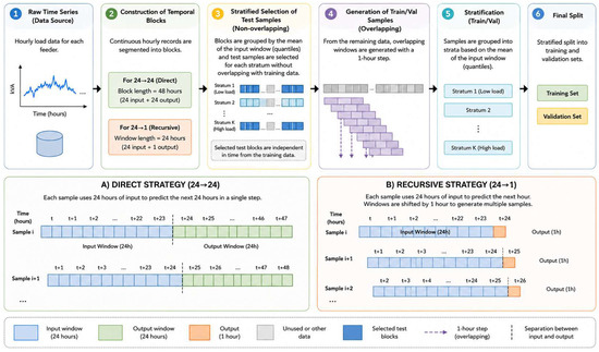
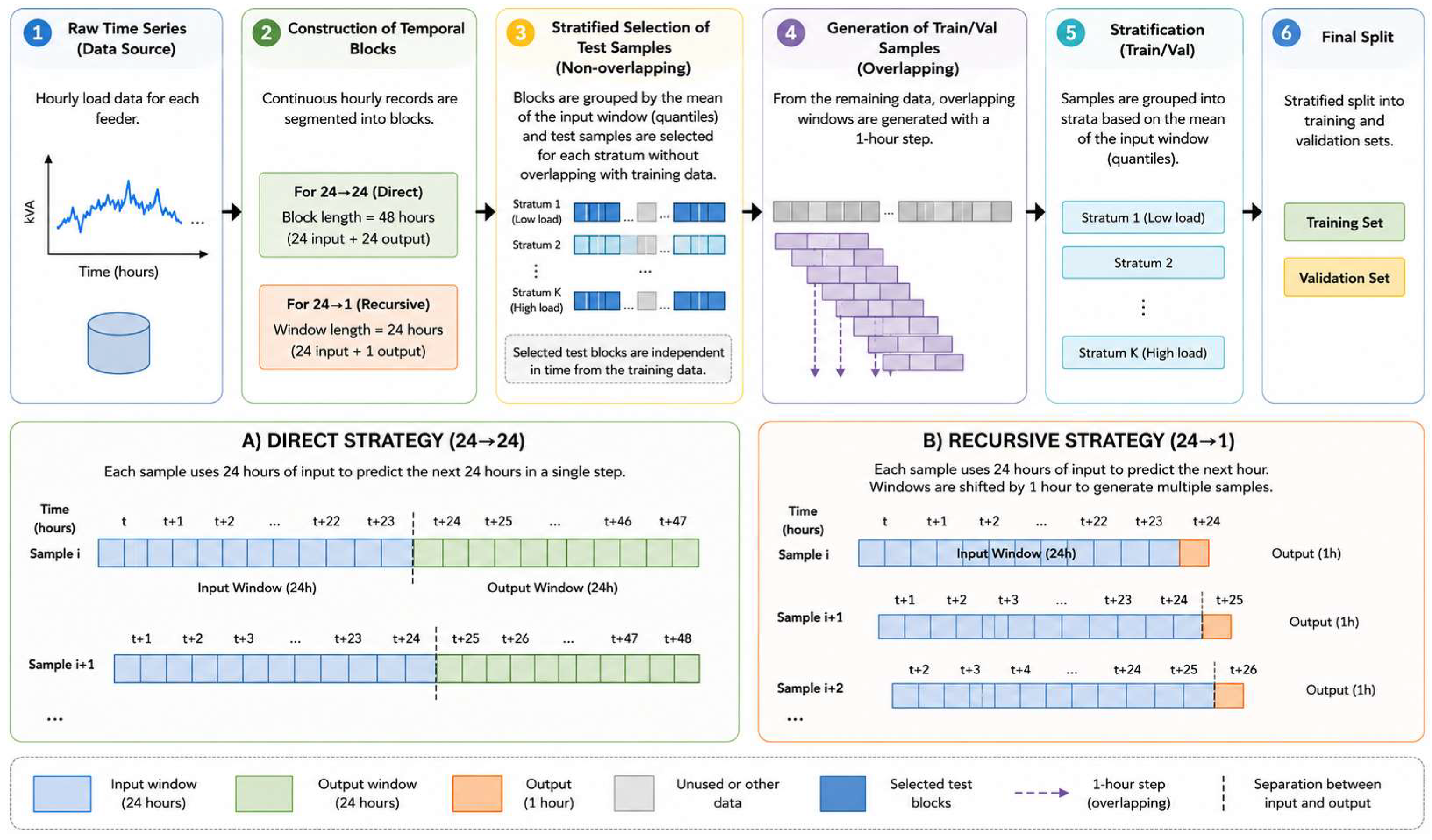
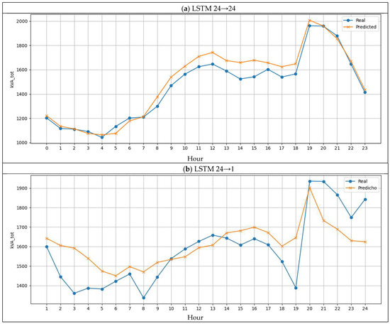
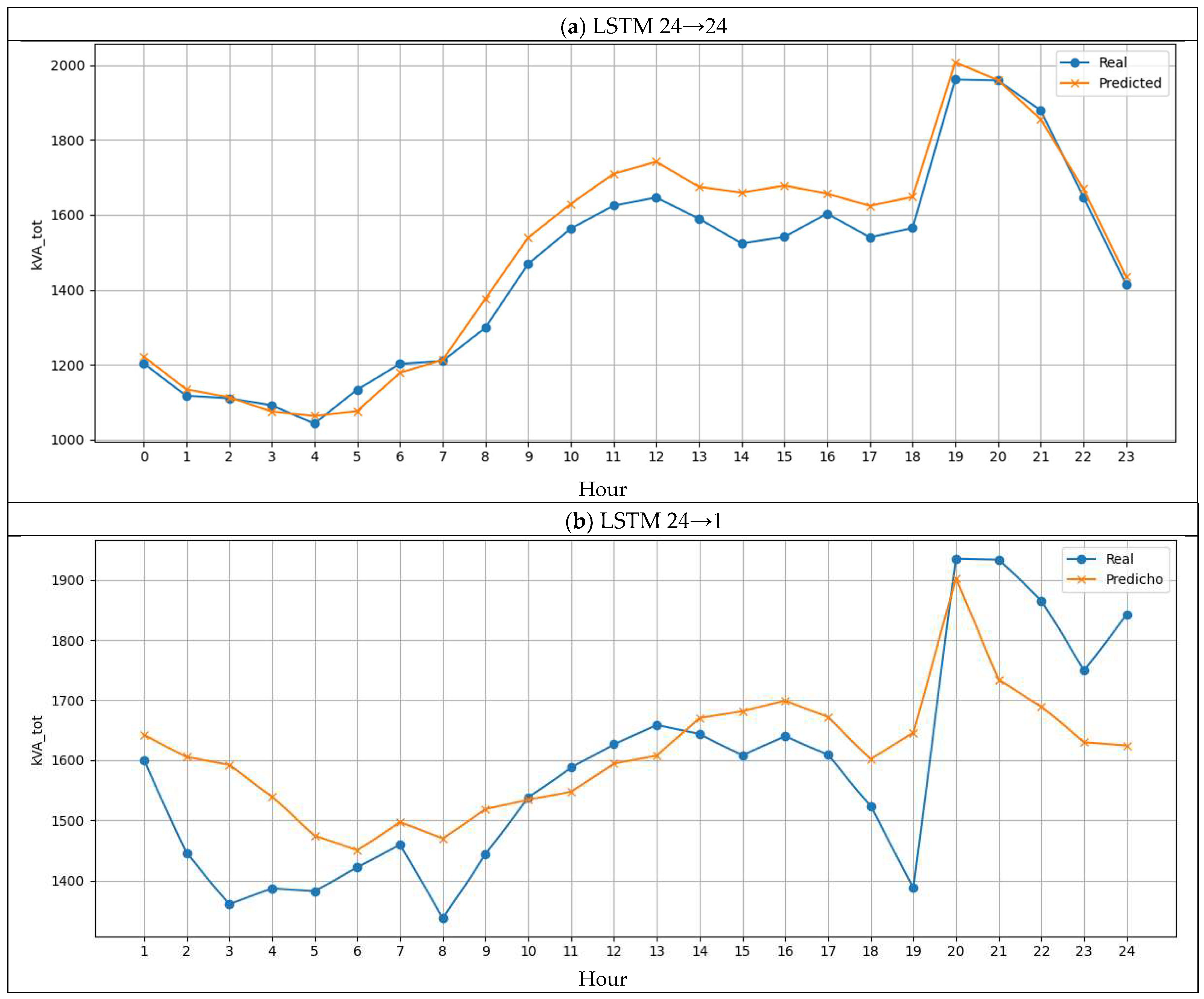
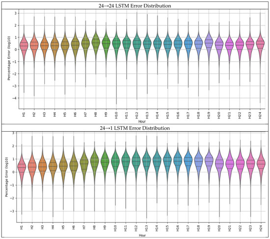
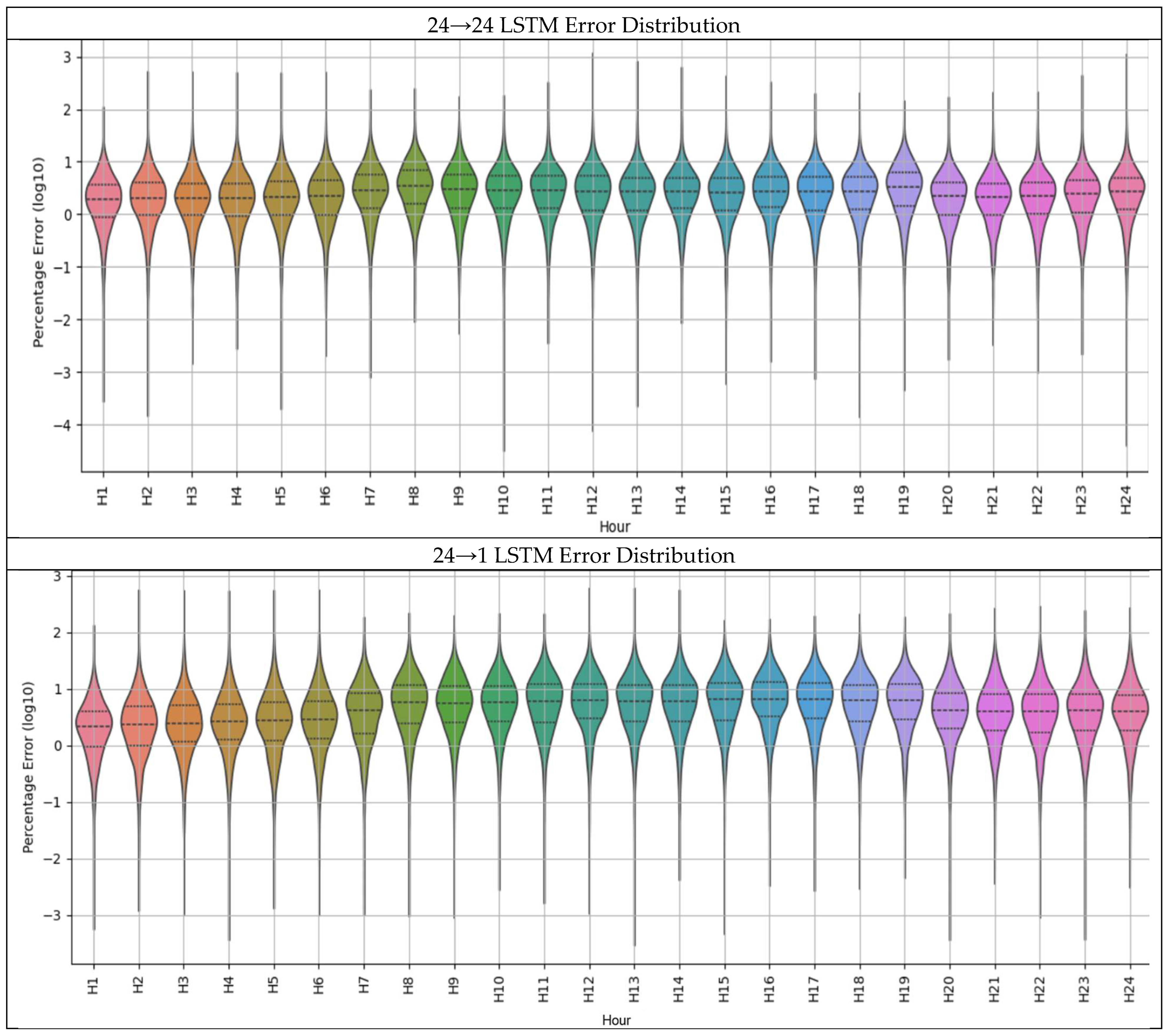
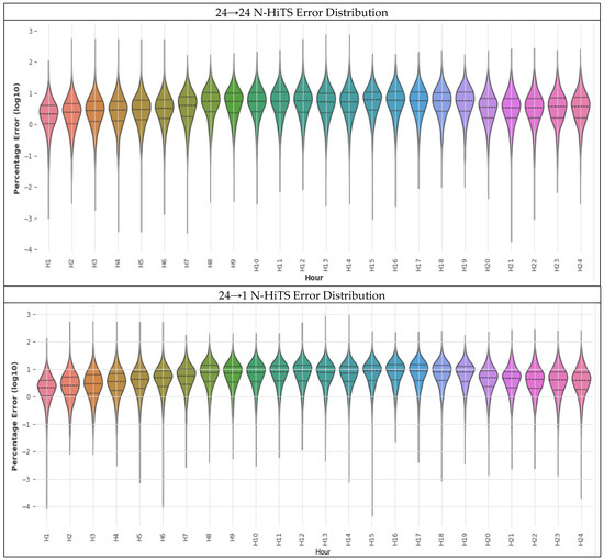
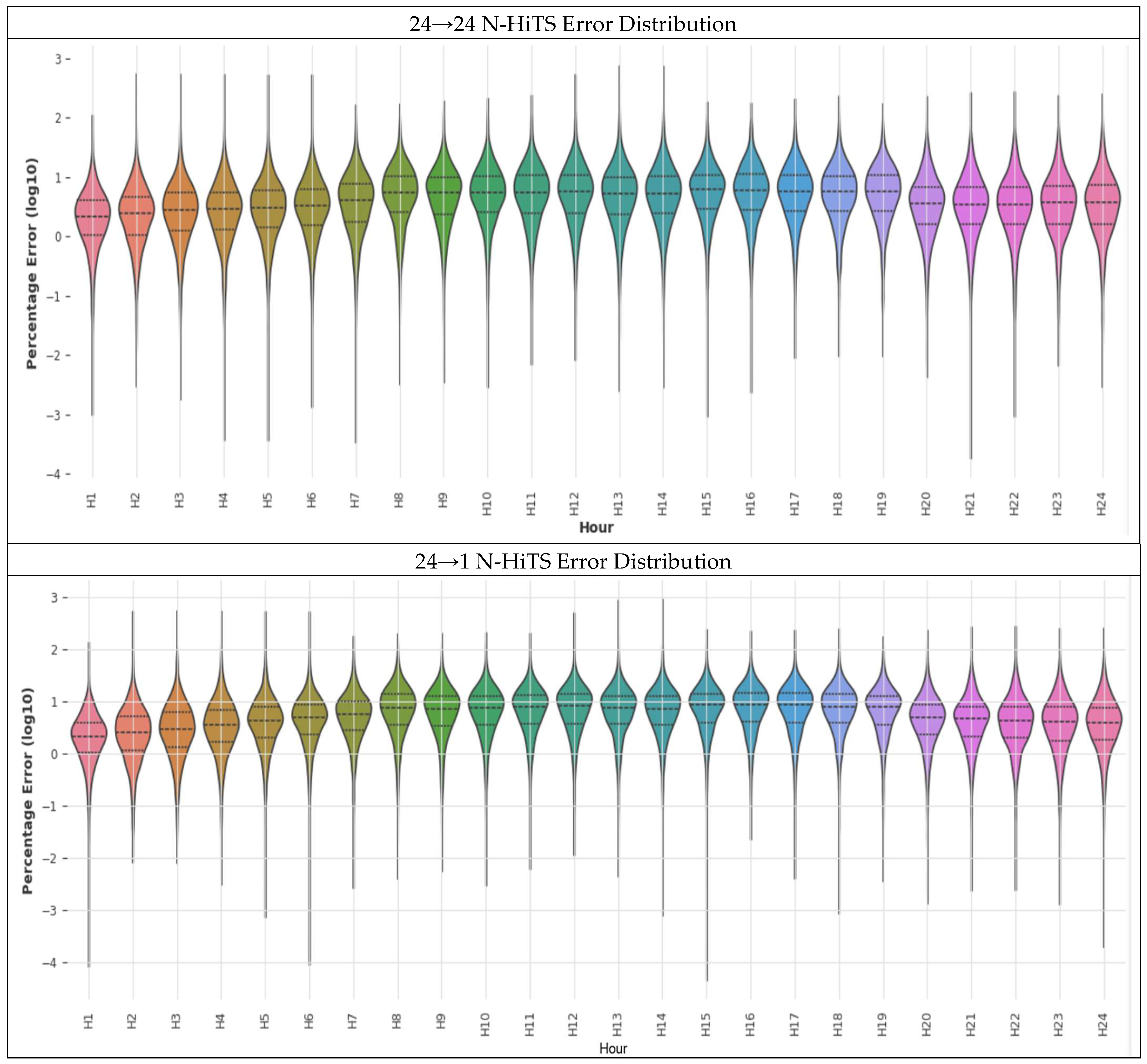
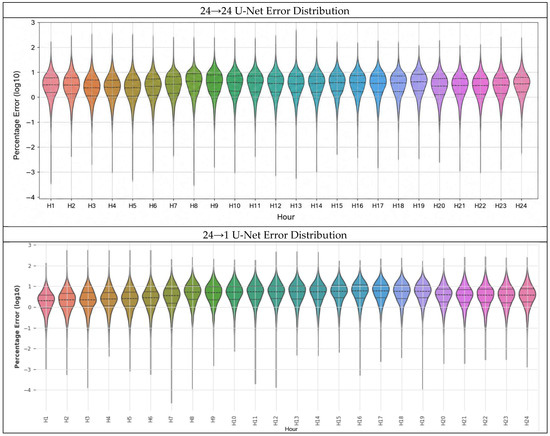
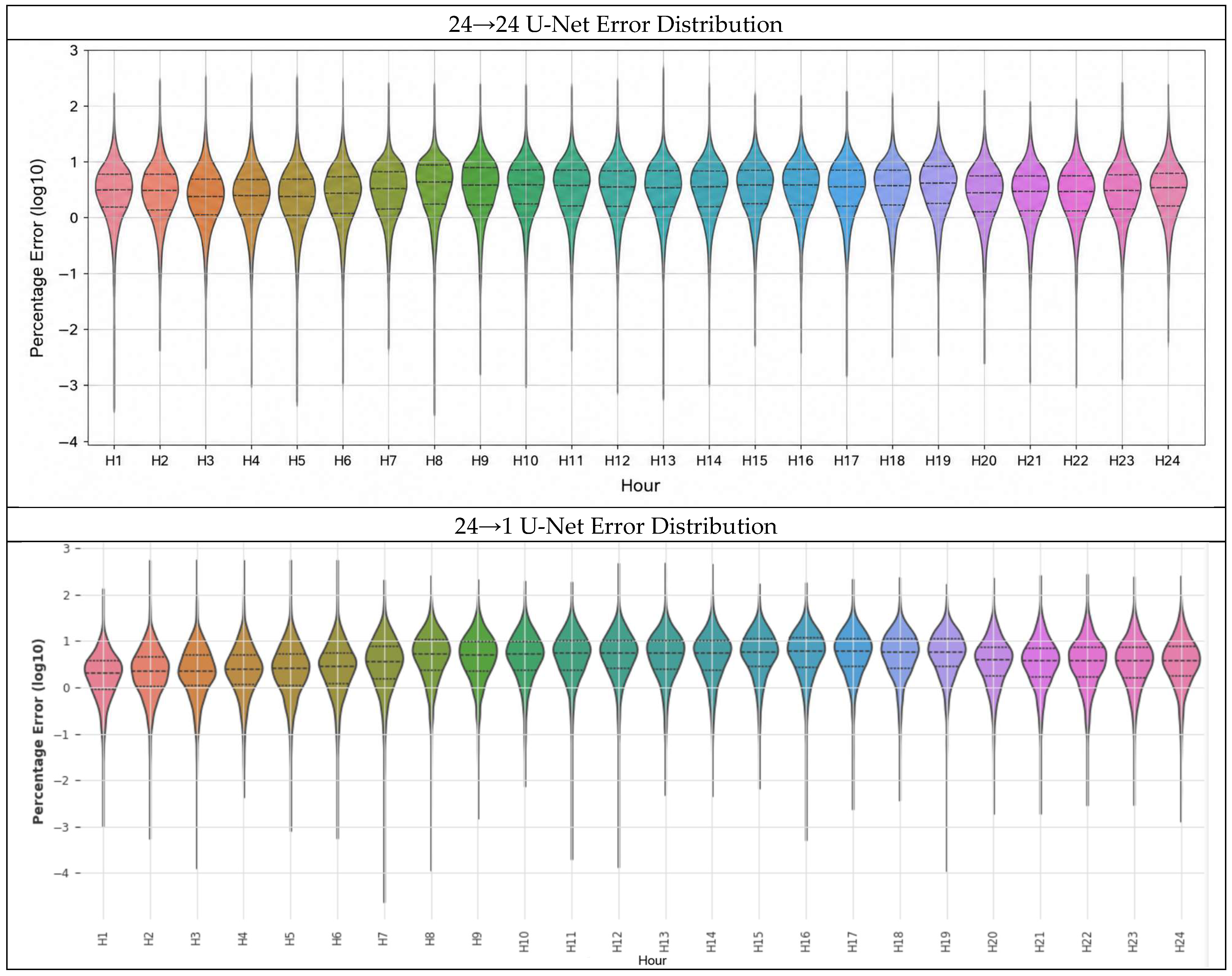
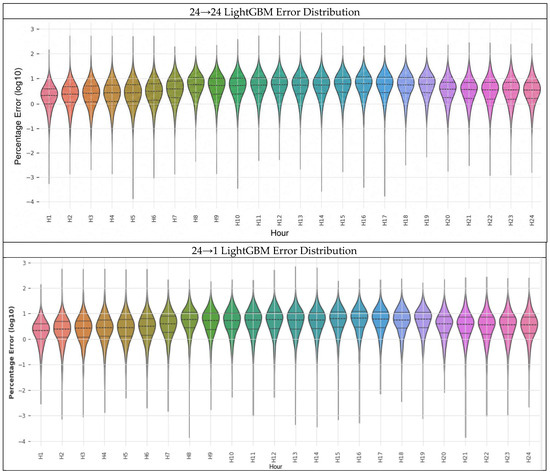
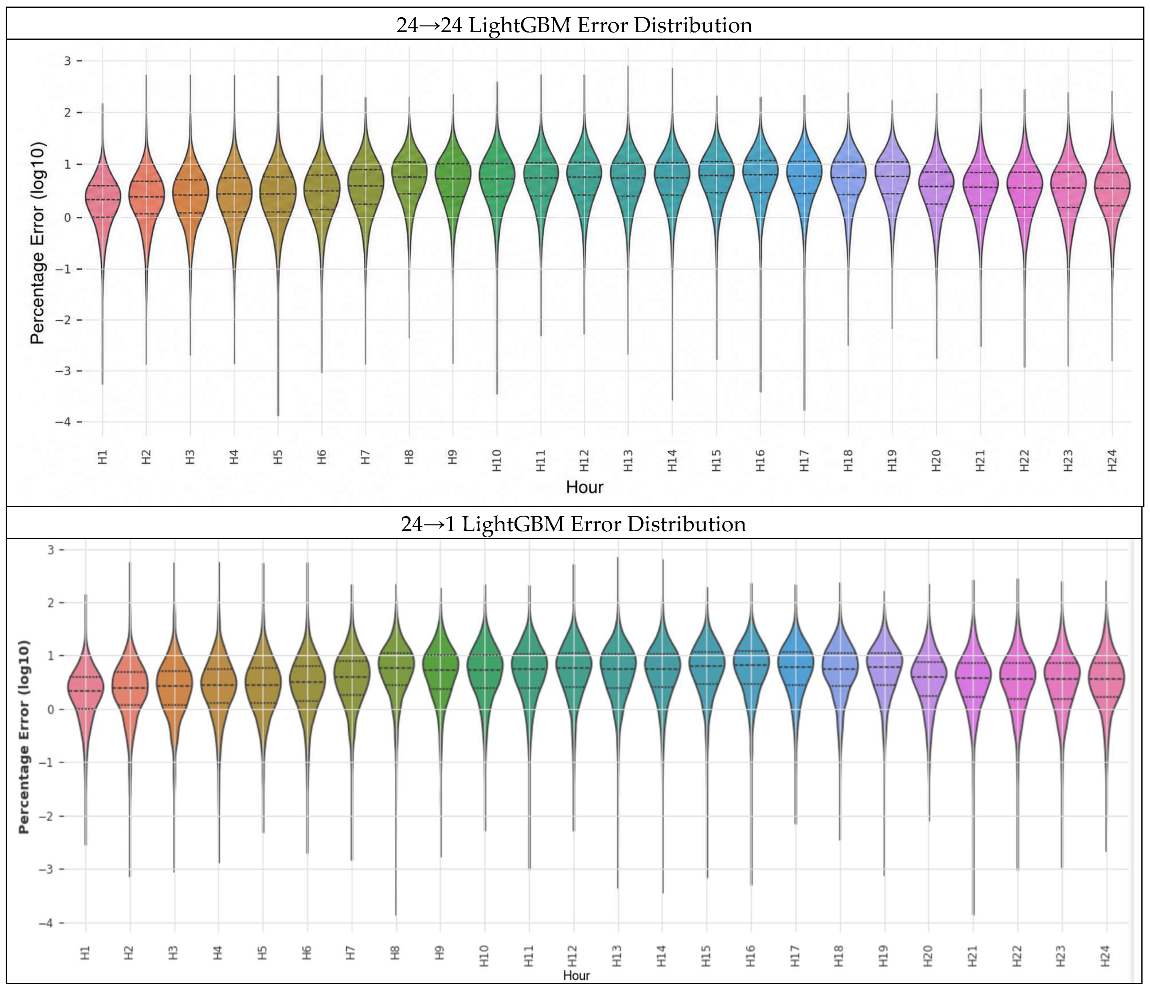
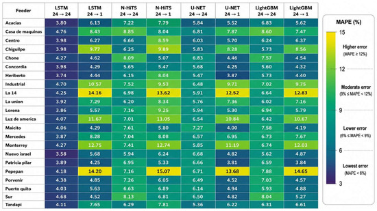
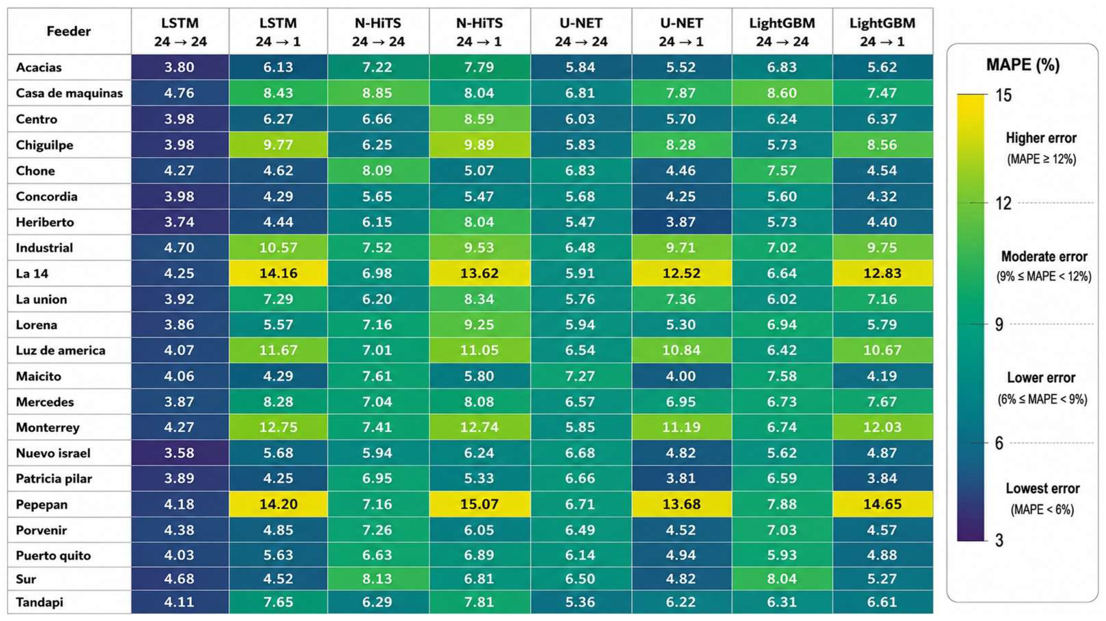
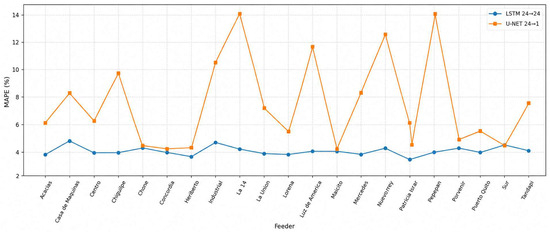
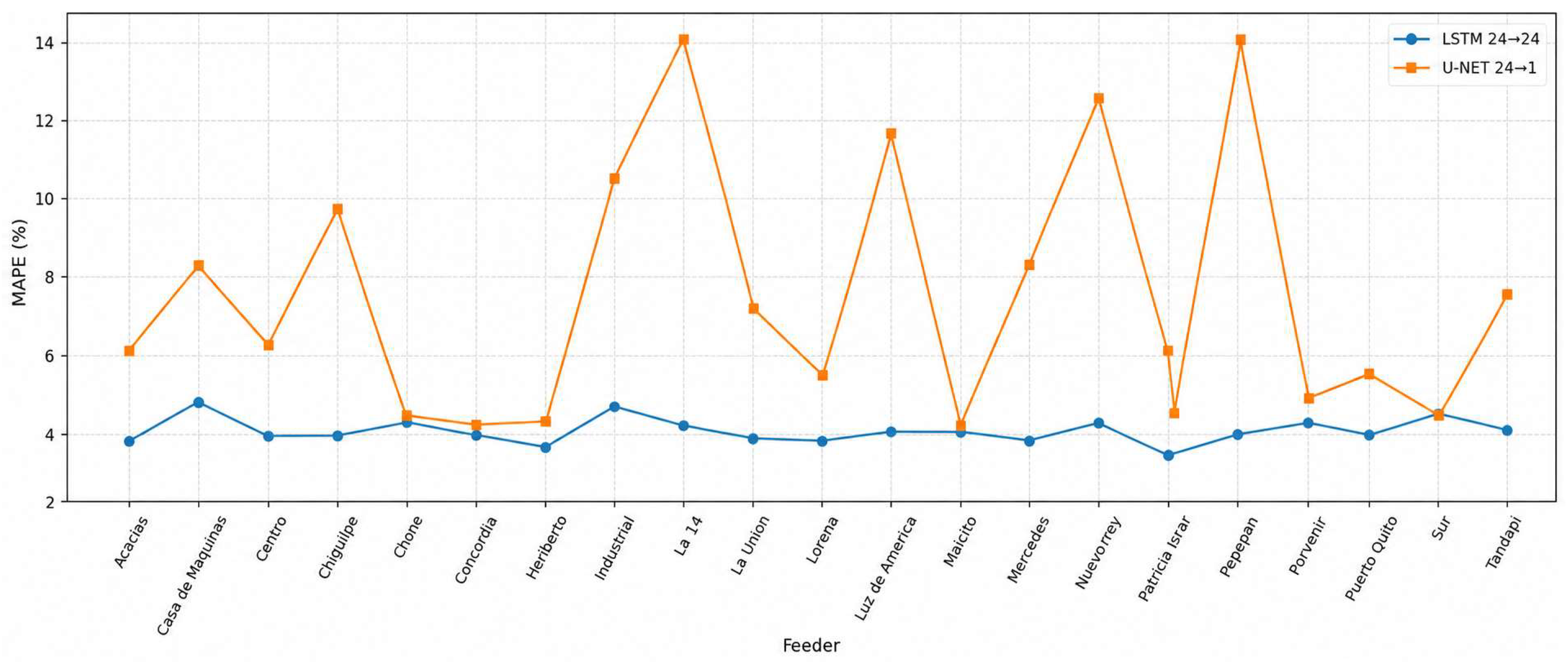
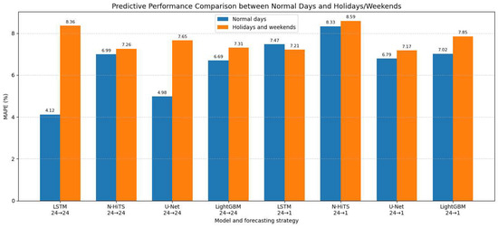
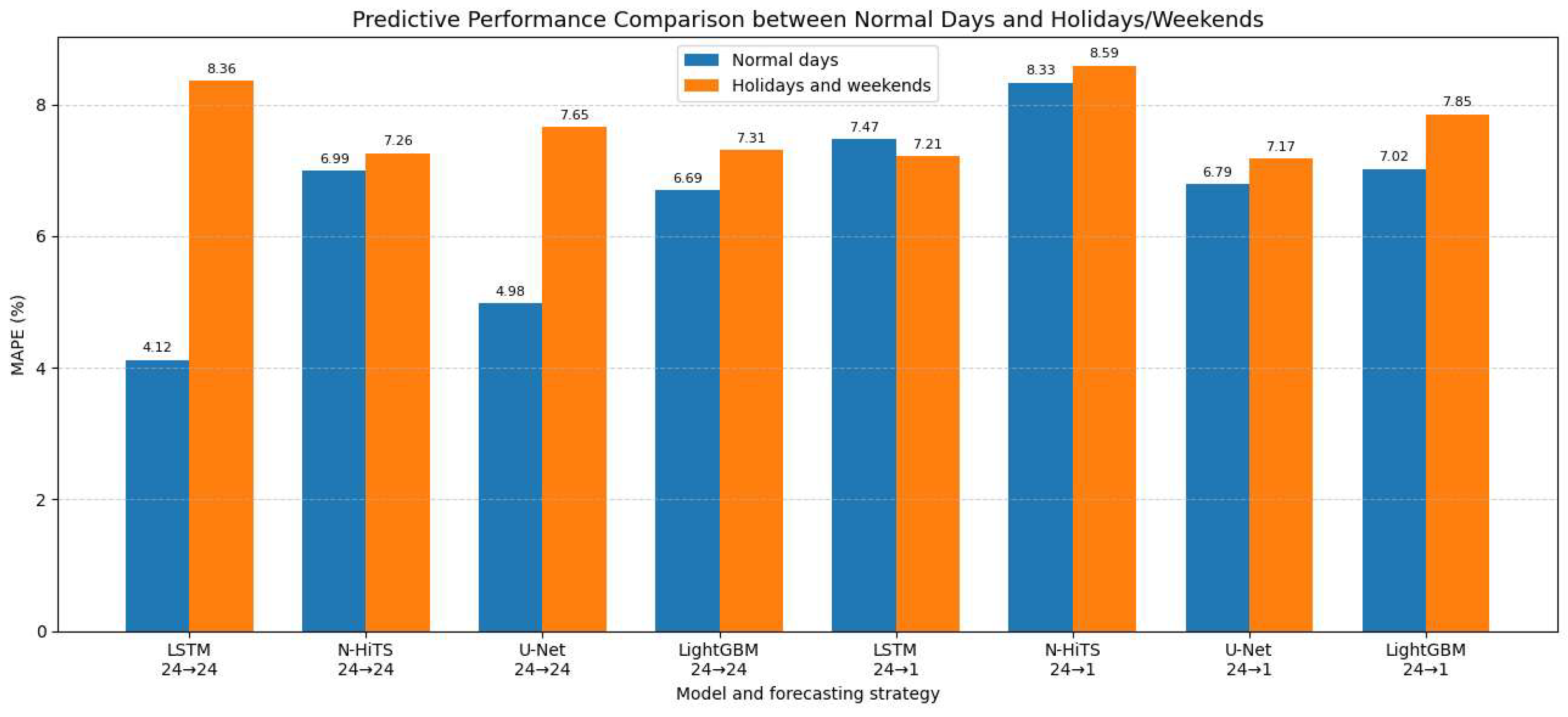
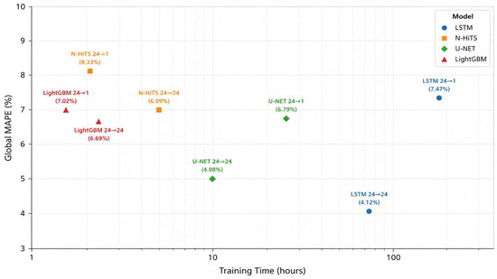
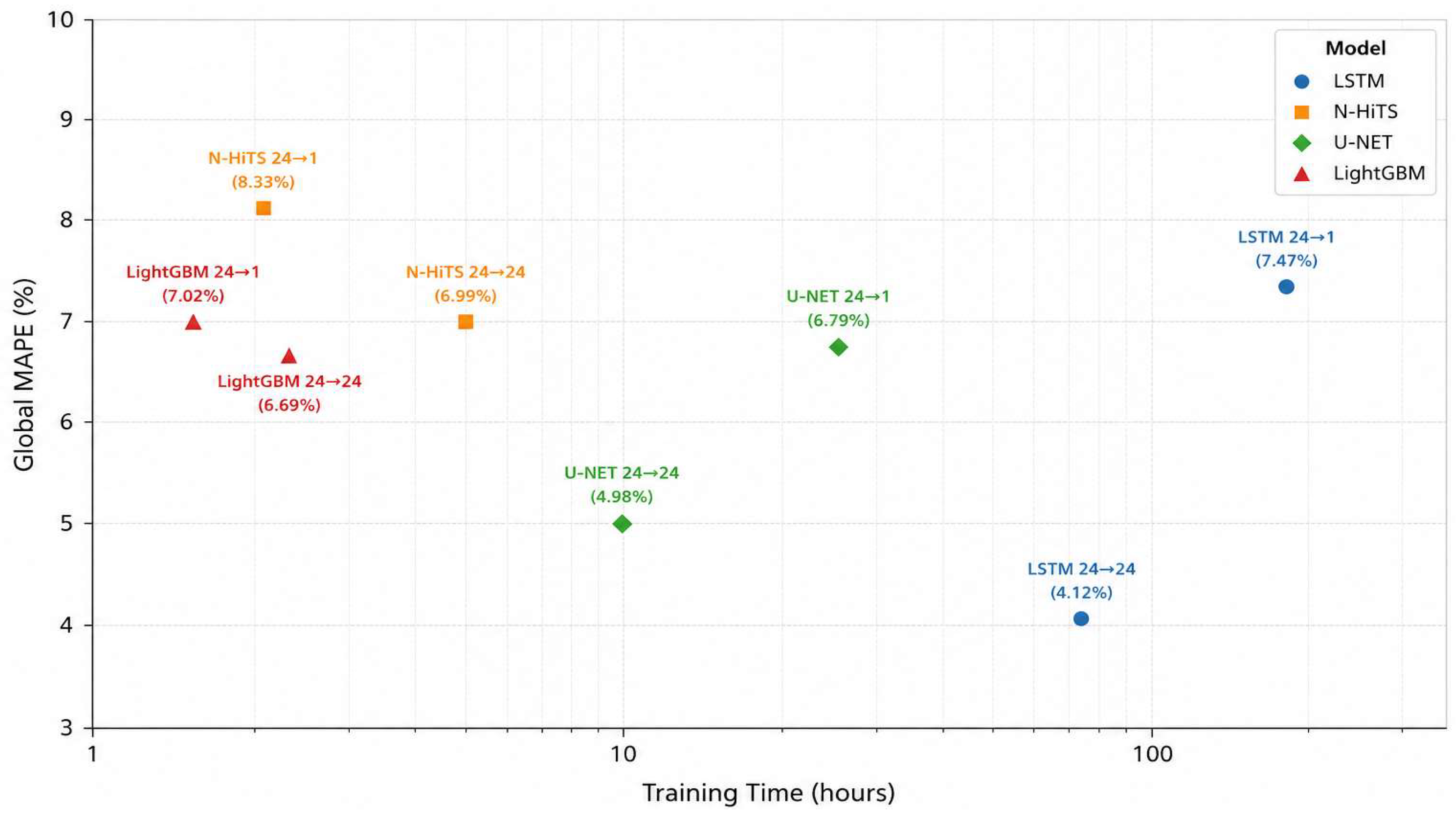

Disclaimer/Publisher’s Note: The statements, opinions and data contained in all publications are solely those of the individual author(s) and contributor(s) and not of MDPI and/or the editor(s). MDPI and/or the editor(s) disclaim responsibility for any injury to people or property resulting from any ideas, methods, instructions or products referred to in the content. |
© 2026 by the authors. Licensee MDPI, Basel, Switzerland. This article is an open access article distributed under the terms and conditions of the Creative Commons Attribution (CC BY) license.