


Abstract
With increasing renewable-energy penetration and power-electronic interfacing, virtual synchronous generators (VSGs) are important inertia-support resources for low-inertia power systems. Existing VSG configuration studies mainly minimize investment cost or treat frequency-security indices as constraints, rather than directly optimizing siting from the perspective of frequency stability. This paper proposes a weighted rate-of-change-of-frequency (w-RoCoF) siting index for VSG configuration. The limitations of center-of-inertia (COI) theory in representing spatial frequency distributions are first analyzed. Then, based on frequency-divider (FD) theory, nodal RoCoF in multi-machine systems is analytically derived, and the w-RoCoF index is formulated to quantify system frequency stability while preserving nodal dynamic information. A multi-objective VSG siting and sizing model considering frequency stability and configuration economy is further established. Case studies on modified IEEE 9-bus and IEEE 39-bus systems show that w-RoCoF identifies critical locations more effectively than the COI index. In the IEEE 39-bus case, the proposed configuration reduces w-RoCoF by 50.7% compared with the cost-oriented scheme and reduces required virtual inertia by 19.7% compared with the frequency-stability-oriented scheme.
1. Introduction
Driven by carbon-peaking and carbon-neutrality targets, renewable-energy-dominated power systems are rapidly developing. With the increasing penetration of renewable generation, conventional synchronous generators are gradually being replaced by inverter-based resources (IBRs). Although this transition is essential for decarbonization, it poses new challenges to secure and stable system operation. Recent frequency-stability incidents worldwide have exposed insufficient inertia support and weakened frequency-response capability in high-renewable power systems [1,2,3]. The declining proportion of synchronous generators reduces system physical inertia and increases frequency-security risks after large disturbances. Moreover, the spatially non-uniform distribution of inertia resources further complicates frequency-stability control [4,5]. Therefore, frequency-support planning should consider not only the overall inertia level but also the spatial distribution of frequency dynamics.
Virtual synchronous generators (VSGs) are widely regarded as effective resources for enhancing frequency stability in low-inertia systems. By emulating synchronous-generator rotor dynamics, VSG-controlled energy-storage systems and other active devices can provide rapid frequency response and virtual inertia support after disturbances, thereby suppressing frequency deviations [6]. Recent advances in battery and energy-storage technologies further support the practical deployment of VSG-controlled storage, although material-level device design is beyond the scope of this study. This capability is particularly important in renewable-energy-dominated systems with reduced physical inertia [7]. Previous studies have shown that VSG-based energy storage can improve frequency-security indicators [8] and reduce frequency fluctuations [9]. Therefore, the proper siting and parameter configuration of VSGs are important for the planning and operation of modern power systems.
Existing VSG and energy-storage configuration studies mainly focus on economic objectives, such as minimizing investment and operating costs, or on conventional planning functions such as energy arbitrage, peak shaving, renewable-power smoothing, voltage-profile improvement, reliability enhancement, and network-loss reduction [10,11,12]. Even when frequency regulation is considered, it is often modeled as a static adequacy constraint, such as requiring sufficient frequency-regulation reserve, rather than as a dynamic-stability objective [13]. Some studies assess frequency stability indirectly through nodal inertia [14,15], but such quasi-steady-state indicators cannot fully capture transient frequency responses after large disturbances. With increasing IBR penetration, post-disturbance dynamic indicators, such as RoCoF for relay-protection settings [16,17] and frequency nadir for under-frequency load-shedding settings [18], should be explicitly considered. Recent studies have incorporated dynamic frequency constraints into VSG planning models, commonly based on center-of-inertia (COI) frequency-response models [19], and some further co-optimize VSG placement and control parameters [20,21]. However, frequency security is still usually treated as a constraint rather than an objective to be directly optimized, and COI-based models cannot represent spatial frequency differences among buses.
A key limitation of these studies is their reliance on the COI model, which assumes a uniform system frequency. When frequency dynamics are spatially non-uniform, lumped inertia models may misrepresent local frequency responses and underestimate frequency-security risks. Therefore, recent studies have begun to investigate node-dependent frequency dynamics. Frequency-divider theory and other analytical frameworks have been proposed to quantify the spatial distribution of RoCoF and frequency deviations at different buses [22,23]. These studies show that local frequency responses may differ significantly from the COI average, highlighting the necessity of considering spatial effects in stability analysis and in the allocation of frequency-support resources such as VSGs. Some studies have derived analytical solutions for two-area frequency dynamics based on modal equations [24,25], and the results indicate that two-area frequency dynamic models can provide more accurate frequency-deviation estimation than the COI model.
The siting and parameter configuration of frequency-support resources should therefore account for spatial frequency dynamics. Based on frequency-divider theory, Ref. [21] calculates nodal RoCoF by allocating the disturbance power among source buses and uses it as a constraint in the configuration problem. However, nodal RoCoF is not further organized into a system-level siting objective. Other studies combine nodal RoCoF with swing equations and use nodal kinetic energy as an optimization objective [26]. Nevertheless, this approach requires repeated solution of differential equations for numerous candidate configurations and disturbance scenarios in a planning problem, which increases the computational burden. For maximum frequency deviation, analytical solutions are available only for simplified two-area systems, while explicit analytical expressions for multi-machine systems remain difficult to obtain [27]. Therefore, a planning-oriented index that preserves nodal frequency information and can be evaluated offline is needed for efficient VSG siting and sizing.
Based on the above analysis, the main innovations and contributions of this paper are summarized as follows:
- (1)
- A weighted RoCoF index is proposed to convert nodal RoCoF information into a system-level siting indicator. Unlike previous studies that mainly use nodal RoCoF as a security constraint, the proposed index directly evaluates the frequency-stability improvement of different VSG placement schemes while preserving spatial frequency-dynamic information.
- (2)
- A VSG siting and sizing model is established by incorporating the proposed w-RoCoF index into the frequency-stability objective. The model simultaneously considers spatial frequency-security performance and configuration cost, so that VSG placement is determined not only by economic cost or feasibility constraints but also by the expected improvement in nodal frequency dynamics.
- (3)
- A contingency-set-based extension is developed to reduce the dependence of the optimal siting result on a single assumed disturbance. The proposed method is verified under different disturbance locations and renewable-energy penetration levels, and the results are further compared with time-domain frequency indicators, including maximum frequency deviation, frequency nadir, and settling time.
The remainder of this paper is organized as follows. Section 2 analyzes the frequency dynamic characteristics of modern power systems and discusses the limitations of COI-based frequency modeling. Section 3 derives the proposed w-RoCoF index based on nodal RoCoF. Section 4 presents the multi-objective VSG siting and configuration model. Section 5 verifies the proposed index and model using modified IEEE 9-bus and IEEE 39-bus systems. Finally, Section 6 concludes the paper. Before introducing the detailed content, this paper first outlines the assumptions and simplifications:
Assumption 1:
Since the index is mainly constructed based on the inertia-response capability of VSGs, the primary frequency-regulation capability of the devices is not considered in the optimization model.
Assumption 2:
While VSG is a versatile control algorithm applicable to various grid-forming converters interfacing DC sources, renewable energy, and energy storage devices, the VSG mentioned in this paper refers specifically to grid-forming energy storage equipped with VSG control, since frequency regulation via primary renewable sources involves significantly more complex dynamics than those of energy storage.
2. Frequency Dynamic Characteristics of Modern Low-Inertia Power Systems
2.1. System Frequency Dynamics Based on the COI Theory
In conventional transient-stability analysis, the overall frequency dynamics of a multi-machine power system are commonly described using the center-of-inertia (COI) theory. This method aggregates the swing motions of multiple synchronous machines into an equivalent single-machine model, thereby providing a simplified representation of the system-level frequency response.
The corresponding swing equation can be expressed as
where Hsys denotes the equivalent inertia constant of the system, Δfsys is the system frequency deviation, f0 is the nominal frequency, Sb,sys is the total rated system capacity, Pd denotes the active-power disturbance, and Δ represents the total primary frequency-regulation power.
The equivalent system inertia and the COI frequency deviation are calculated as
where the subscript g denotes the g-th inertia-providing generation unit. Hg, Sb,g, and Δfg denote its inertia time constant, rated capacity, and frequency deviation, respectively.
The COI equation represents the overall frequency acceleration or deceleration of a power system by aggregating a multi-machine system into an equivalent inertia model. Although effective for synchronous-generator-dominated systems, the COI frequency is a global inertia-weighted average rather than the actual frequency at any specific bus. Therefore, it cannot accurately capture local frequency-stability issues caused by spatially non-uniform inertia and network topology.
2.2. Spatial Characteristics of Frequency Dynamics in Power Systems with High Renewable-Energy Penetration
In an actual power system, especially during the transient process after a large disturbance, the frequency is not identical everywhere in the system. For different nodes in the power grid, the rate of change and magnitude of frequency differ owing to their line-connection structures and their relative locations with respect to the disturbance. When a disturbance occurs, the bus frequency near the disturbed bus first changes sharply and then propagates outward through the electromechanical coupling of the grid. For example, a local power deficit may cause an abrupt frequency drop in that area, whereas the frequency variation in regions far from the disturbed bus or with larger inertia is much milder.
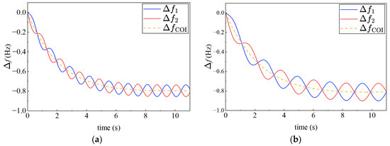
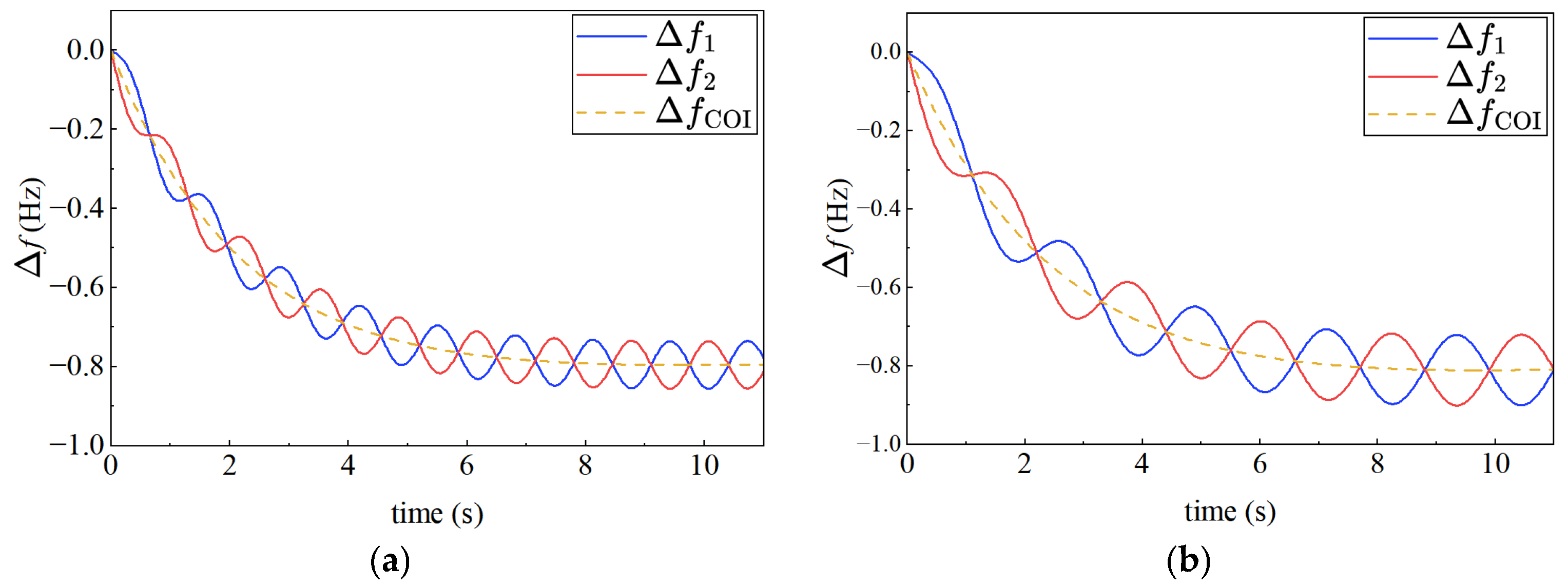
This phenomenon becomes more pronounced in power systems with high renewable-energy penetration. Figure 1a shows the frequency dynamics of an actual two-area system, and Figure 1b shows the results after increasing the tie-line impedance between the two areas. In this system, renewable inertia resources and loads are concentrated in two different areas, which can be regarded as a two-node system. It can be observed that weaker coupling leads to larger inter-area oscillation amplitudes. This is because significant regional differences in inertia amplify the differences in regional frequency dynamics, especially when generator tripping occurs in a low-inertia area [28]. This indicates that the distributed nature of renewable energy further increases inertia non-uniformity, making local frequency dynamic differences in the system more prominent.
Figure 1.
Frequency responses of the two-area system under different coupling conditions: (a) frequency response with relatively strong coupling; (b) frequency response with relatively weak coupling.
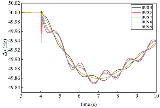
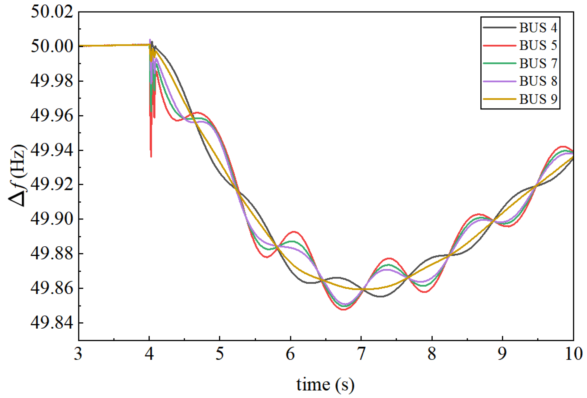
To more intuitively illustrate the spatial differences in system frequency after integration of power-electronic-interfaced equipment, a simulation was performed on the IEEE 9-bus test system in PSCAD. The simulation corresponds to the 30% renewable-energy penetration case described in Section 4.2. Figure 2 shows the frequency-response curves measured at different buses after an active-power disturbance is applied at one bus in the system. It can be observed that the frequency dynamics of different buses do not coincide. At the disturbance instant, the frequency deviation amplitude at Bus 5 is significantly larger than the amplitudes at the other buses, and its frequency nadir is approximately 49.85 Hz, which is lower than the nadirs observed at the other buses.
Figure 2.
Frequency response of the IEEE 9-bus system.
The above spatiotemporal differences in nodal frequency indicate that, when analyzing the large-disturbance transient process of a power system, the classical COI model, which represents the entire system using a single frequency, is no longer applicable. To accurately characterize the dynamic behavior of each bus and its influence on system stability, it is necessary to establish the swing equation for inertia-providing buses, such as buses equipped with synchronous generators or VSGs. For a generator bus g in the power system, the swing equation is given by:
By comparing Equations (1) and (4), it can be observed that, when the disturbance location changes, the disturbance-power term ΔPd in Equation (1) cannot distinguish the influence of different disturbance locations. Therefore, the frequency dynamics described by the COI theory cannot reflect frequency variations caused by different disturbance locations. In other words, the COI frequency describes the equivalent rotor-motion state obtained by the weighted average of all generator rotors, thereby ignoring local frequency dynamic characteristics. In contrast, for Equation (4), the power-imbalance term ΔPd,g varies with the disturbance location.
In summary, the COI frequency is a global averaged quantity and may underestimate RoCoF and frequency-deviation risks at weak buses. Therefore, network topology and nodal frequency differences should be considered when evaluating local frequency stability and planning frequency-support resources. To compare different VSG configuration schemes using a system-level index, two questions are raised: (1) how to establish a frequency-security index that reflects nodal dynamic characteristics; and (2) how to quantify nodal frequency differences within this index.
3. Siting Index Based on Nodal RoCoF
To address the questions raised in Section 2, this section proposes a new frequency-security siting index from the perspective of nodal frequency-security indicators. For large-scale systems, nodal Δfmax cannot yet be calculated analytically, whereas nodal RoCoF can be obtained for all network nodes by calculating the allocation of the initial disturbance. In addition, maximum RoCoF is commonly used in engineering practice to estimate Δfmax [29], demonstrating the engineering practicality and importance of RoCoF. Therefore, this section first derives the calculation of nodal RoCoF and then presents the formulation of the proposed siting index.
3.1. Derivation of Nodal RoCoF
For a transmission network with relatively long lines, the line impedance is generally dominated by reactance. Under this assumption, the nodal voltage equation of the network can be established using the susceptance matrix [30]:
Furthermore, if the transient reactances of synchronous generators and other generation units are considered, and the nodal voltage equation is partitioned according to generator buses and network buses, Equation (5) can be augmented as
where is the augmented susceptance matrix; and are the current vectors injected into generator buses and network buses, respectively; and and are the internal electromotive-force vector of the generators and the voltage vector of the network buses, respectively; BGG is the susceptance matrix composed of generator transient reactances and is diagonal; is also formed from generator transient reactances and is extended from BGG to have the same dimensions as B; BGB and BBG are the mutual susceptance matrices connecting generator transient reactances with network buses, and they are transposes of each other; and B is the original network susceptance matrix. When a power disturbance occurs in the network, to eliminate the influence of other unobserved nodes, the augmented susceptance matrix in Equation (6) is reduced, retaining only the generator nodes and disturbance nodes [31], which yields
where the subscript C denotes the set of retained buses, whereas R denotes the set of remaining buses to be eliminated. After the rows and columns of the augmented susceptance matrix are reordered according to the retained and eliminated bus sets, BCC is the self-susceptance submatrix associated with the retained buses, and BRR is the self-susceptance submatrix associated with the eliminated buses. BCR and BRC are the mutual susceptance submatrices between the retained and eliminated buses. This reduced matrix is then used to calculate the active-power imbalance allocated to each inertia-providing generation bus.
When a power imbalance occurs at a bus in the power system, primary frequency regulation has not yet responded during the initial stage of the disturbance. Therefore, according to Equation (4), the swing equation of inertia-providing generation unit g can be written as
where ΔPd,g denotes the active-power imbalance allocated to generation unit g at the disturbance instant. A negative value of ΔPg indicates an active power deficit. To calculate the RoCoF of each generation bus at the disturbance instant, the active-power imbalance allocated to each inertia-providing generation unit must first be determined. According to [31], this allocation can be expressed as
where M denotes the number of inertia-providing generation units, ΔPd,j is the active-power imbalance at bus j, and Sg,j is the synchronizing power coefficient between source bus g and network bus j. Eg0 denotes the initial internal electromotive force of source bus, while Vj0 denotes the initial voltage of network bus j. Δδg and Δθj denote the power-angle variation of source bus g and the voltage-angle variation of bus j, respectively.
At the initial instant following a disturbance, voltage magnitudes and rotor-angle variations are still small. Therefore, the internal electromotive forces of all source buses and the bus voltages are set to 1.0 p.u., and the nonlinear synchronizing-power coefficients are approximated by linear allocation factors determined by the susceptance matrix. This approximation is commonly used in frequency-divider-based and small-signal frequency-response studies and introduces only small errors in initial RoCoF estimation under normal operating conditions. Consequently, the allocation factor can be simplified as
During the initial inertial response stage, the mechanical output power of each generation unit is assumed to remain unchanged, the frequency deviation has not yet developed sufficiently, and primary frequency response has not yet been activated. Since damping and voltage dynamics mainly affect the subsequent frequency nadir and recovery process rather than the initial RoCoF, and previous studies have shown that neglecting damping can still provide high accuracy in frequency-response calculation [32], the damping term in Equation (8) is omitted here. By combining Equations (8) and (9), the RoCoF of the inertia-providing generation buses can be obtained as
where ΔfG, ΔPd,G, HG, and Sb,G denote the column vector of generator-bus RoCoF, the column vector of active-power imbalance allocated to the generation buses, the diagonal matrix of inertia time constants, and the diagonal matrix of rated capacities, respectively.
According to frequency-divider theory [23], once the frequency dynamics of the inertia-providing generation buses are known, the frequency dynamics of the remaining network buses can also be obtained. Therefore, the initial RoCoF values of the non-generation buses can be calculated as
where denotes the initial RoCoF vector of the remaining network buses. It can be observed that the RoCoF of a network bus is determined by the inertia time constants of the generation buses, the topological relationship between the network buses and the generation buses, and the location of the disturbance.
Combined with the analysis in Section 2, this indicates that frequency dynamics exhibit clear spatial characteristics. Equipping the selected bus with a VSG not only changes its equivalent inertia, but also affects the corresponding elements of the network admittance matrix. Therefore, when the VSG placement location differs from the disturbance location, the frequency stability of some buses may deteriorate after configuration. This phenomenon will be demonstrated in the case studies.
3.2. Construction of the System Weighted RoCoF Siting Index
The purpose of the proposed index is to evaluate the overall frequency-stability level of the system when frequency-support resources are limited. It is designed to address the two issues raised at the end of the preceding section. First, the index should retain the information of local frequency dynamics. Second, it should provide a unified system-level metric for comparing different VSG siting schemes. In addition, the index should be calculable offline without relying on time-domain simulations. This is particularly important because the maximum nodal frequency deviation generally requires time-domain simulation, whereas nodal RoCoF can be obtained analytically using the derivation presented above.
Based on the nodal RoCoF derived in Section 3.1, the RoCoF values with and without VSG deployment are distinguished and used to construct a comprehensive evaluation index:
where w-RoCoF denotes the weighted rate of change of frequency. RoCoF0,i represents the RoCoF of bus i after the disturbance before VSG placement, whereas RoCoFi represents the RoCoF of bus i with a VSG deployed at a candidate location. It should be emphasized that RoCoF0,i is not the RoCoF under an undisturbed operating condition. Instead, it is the nodal RoCoF immediately after the disturbance but before VSG deployment. Therefore, RoCoF0,i represents the original frequency vulnerability of bus i under the considered contingency. By using RoCoF0,i as the weight, the proposed index gives higher priority to buses with more severe pre-deployment frequency dynamics, while RoCoFi evaluates the post-deployment frequency-security performance. In this way, the w-RoCoF index can reflect whether a VSG configuration effectively improves the buses that are originally more vulnerable to frequency disturbances.
By weighting nodal RoCoF values, the proposed w-RoCoF index retains local frequency-dynamic information that is ignored by the conventional COI-based index. It also reduces the masking effect caused by simple system-level averaging under uneven inertia distribution. Therefore, the proposed index links nodal frequency behavior with system-level VSG allocation and provides a more suitable metric for frequency-stability-oriented siting.
4. w-RoCoF-Based VSG Configuration Optimization Model
The configuration of virtual synchronous generators should simultaneously account for local frequency dynamics and overall system frequency stability. In this section, the spatial distribution characteristics of frequency dynamics are considered, and a VSG siting and configuration model is established by minimizing the weighted rate of change of frequency.
4.1. Decision Variables
The VSG siting and parameter configuration problem is a typical mixed-integer nonlinear programming problem. The decision variables of the proposed model are defined as follows.
First, the siting variable is defined as a binary variable set:
where Ωc denotes the set of candidate buses for VSG deployment. zk = 1 indicates that a VSG is deployed at bus k, whereas zk = 0 indicates that no VSG is deployed at this bus.
Second, the virtual inertia decision variable is defined as a continuous variable coupled with the siting variable:
where EVSG,k denotes the virtual inertia of the VSG deployed at bus k. When zk = 0, EVSG,k = 0; HVSG,k represents the virtual inertia time constant of the VSG; SVSG,k represents the rated apparent power of the VSG.
Therefore, the complete decision vector can be written as X = [Z,Em,VSG]. If zk = 1, a VSG is configured at bus k, and the total number of inertia-providing generation units in the system increases from M to M’ = M + 1. Meanwhile, the type of bus k changes from a non-inertia bus to an inertia-providing source bus. According to the derivation in Section 3.1, the frequency characteristics of bus k are no longer determined only by other inertia-providing buses. Instead, bus k actively responds to the active-power imbalance during the inertial response stage and shares part of the disturbance power. Consequently, both the nodal RoCoFk and the system w-RoCoF are changed.
4.2. Objective Functions
The first objective is to improve the frequency-stability performance of the system. When VSGs are deployed at different buses, the equivalent inertia and bus type of the selected buses change, which further changes the nodal RoCoF values. Therefore, the w-RoCoF index proposed in Section 3.2 is selected as the frequency-stability objective:
The deterministic formulation above evaluates the frequency-security performance of a VSG configuration under a specified disturbance. However, in practical planning studies, the optimal placement may depend on the disturbance location, renewable-energy penetration level, and operating condition. To avoid obtaining a configuration that is optimal only for one assumed disturbance, the proposed model can be extended to a contingency-set-based planning formulation. Let Ωs denote the predefined contingency set. Each scenario s is characterized by the disturbance bus, active-power imbalance, renewable-energy penetration level, and operating condition. This can be written as:
where bs is the disturbed bus, ΔPs is the active-power disturbance, λs is the renewable-energy penetration level, and ρs is the weighting factor of scenario s. For a given VSG configuration X, the w-RoCoF index is calculated separately under each contingency scenario:
To consider both the overall performance and the most severe contingency, the frequency-stability objective is reformulated as a combination of the expected w-RoCoF over the contingency set and the worst-case w-RoCoF:
where η ∈ [0,1] is a trade-off coefficient. In this study, η is set to 0.7 to emphasize the average frequency-security improvement while still penalizing the worst contingency.
In practical applications, a larger VSG inertia generally requires a higher investment cost. From the planning perspective, the total investment cost should be kept as low as possible. In this study, the investment cost is assumed to be proportional to the configured virtual inertia. Therefore, minimizing the investment cost is equivalent to minimizing the total configured VSG inertia:
Equations (16) and (17) constitute a multi-objective optimization problem with two conflicting objectives in different dimensions. Conventional solution methods usually calculate the complete Pareto-optimal front and then select one solution from it. However, this process can be computationally expensive. To reduce the computational burden, a compromise-based approximate solution method is adopted following [33]. Let F1(x1*) and F2(x2*) denote the optimal values obtained when Equations (16) and (17) are solved separately. The original multi-objective optimization problem can then be transformed into the following single-objective optimization problem:
where Δd denotes the difference between the distance from a solution point to the ideal point and the distance from the same point to the worst point. d+ is the distance from the solution point to the ideal point, and d- is the distance from the solution point to the worst point. The detailed derivation of this transformation is provided in Appendix A.
4.3. Constraints
For the VSG configuration problem, the main constraints considered in this study include the RoCoF constraint, the frequency-deviation constraint, and the virtual inertia limit. At the instant of a disturbance, primary frequency regulation and other slow dynamic processes have not yet responded. Therefore, the slow dynamic variables during the inertial response stage can be neglected, and the maximum RoCoF is generally assumed to occur at the disturbance instant. Although the system-level w-RoCoF is used as the objective function, the RoCoF of an individual bus may still exceed the allowable limit. Therefore, the RoCoF of bus i should satisfy
where RoCoFmax denotes the maximum allowable RoCoF limit, which is generally taken as 0.5 Hz/s according to the relevant standard [18]. It should be noted that the RoCoF constraint is imposed on the post-deployment nodal RoCoF values under each candidate VSG configuration. If some buses exceed the RoCoF limit before VSG deployment, the initial system is regarded as frequency-insecure rather than infeasible for the planning problem. The purpose of the optimization is then to find a VSG configuration that reduces the nodal RoCoF values and makes the post-deployment system satisfy the prescribed limit. Therefore, feasibility is judged according to the RoCoF values after VSG configuration.
The system RoCoF calculated using COI theory is not considered as an additional constraint. This is because, according to the COI formulation, the COI-based system RoCoF lies between the RoCoF values of the inertia-providing buses. Therefore, when all nodal RoCoF values satisfy the constraint, the COI-based system RoCoF also satisfies the constraint.
Similarly, to prevent excessive frequency deviation from causing frequency instability, the frequency deviation should satisfy
where ∆fmax denotes the maximum allowable system frequency deviation, and this constraint ensures that the frequency deviation of the system remains within the permitted range.
Since the virtual inertia of a VSG is adjustable, its virtual inertia constant is constrained by the converter capacity and economic operation considerations. Therefore, the virtual inertia constant of the VSG should satisfy
where HVSG,min and HVSG,max denote the lower and upper limits of the VSG inertia time constant, respectively. The value of HVSG,max is constrained by the capacity and control capability of the converter.
4.4. Solution Procedure for the VSG Siting and Configuration Model
Based on the above formulation, the VSG siting and configuration model considering spatial frequency characteristics can be expressed as
Equation (25) constitutes the proposed VSG siting and configuration optimization model. With the spatial characteristics of frequency dynamics taken into account, the post-disturbance system w-RoCoF is adopted as the optimization objective, while nodal RoCoF, nodal frequency, and equipment-parameter constraints are simultaneously considered. Accordingly, the siting locations and parameters of VSGs are optimized to improve the overall frequency-stability performance of the system.
Since the proposed model contains discrete siting variables and continuous sizing variables, it can be solved by different optimization methods, such as enumeration, mixed-integer programming, or metaheuristic algorithms. In this paper, a population-based optimization method [34] is adopted as a numerical solver to obtain the VSG siting and sizing results. The main focus of this study is the proposed w-RoCoF-based planning model rather than the development of a new optimization algorithm.
Step 1: Initialization. Set the population size Q, the maximum number of iterations Tmax, and the stagnation threshold Ns. Each individual represents a candidate VSG configuration, Xi = [zi,1,...,zi,k,Ei,1,...,Ei,k], where zi,k∈{0,1} is the siting variable and Ei,k is the configured VSG inertia at candidate bus k. The initial population is randomly generated within the feasible ranges of z and E.
Step 2: Fitness evaluation. For each individual Xi, decode the binary siting variables and continuous inertia variables to obtain a VSG configuration scheme. The nodal RoCoF values and the corresponding w-RoCoF objective are then calculated. Constraint violations, including the maximum number of VSGs, the inertia limits, and the nodal RoCoF limits, are handled by a penalty function. The fitness function is written as:
where F(Xi) is the objective value of the configuration model, P(Xi) is the total normalized constraint violation, and μ is the penalty coefficient.
Step 3: Position update. After all individuals are evaluated, the three best individuals are selected and denoted as Xα, Xβ, and Xδ. The position of each individual is updated according to the grey-wolf search rule:
For the binary siting variables, a Sigmoid mapping is used:
The continuous inertia variables are directly limited to their lower and upper bounds.
Step 4: Constraint repair. If the number of selected VSG buses exceeds the allowed maximum, only the buses with the largest corresponding inertia values are retained. If a selected bus has an inertia value outside the allowable range, it is corrected to the nearest bound.
Step 5: Termination. Steps 2–4 are repeated until the maximum iteration number Tmax is reached or the best solution remains unchanged for Ns consecutive iterations. In this study, Q = 50, Tmax = 100, and Ns = 20.
5. Case Studies
In this section, the proposed w-RoCoF index is first verified using the IEEE 9-bus system. Three frequency-security assessment indices are compared, and PSCAD simulations are conducted to obtain the maximum frequency deviation at each bus as a reference metric for evaluating the effectiveness and superiority of the proposed w-RoCoF index. The corresponding VSG siting characteristics are then analyzed.
The three indices are defined as follows:
Index 1 (I1): RoCoF calculated based on COI theory;
Index 2 (I2): system average RoCoF calculated using nodal RoCoF;
Index 3 (I3): the proposed w-RoCoF.
Furthermore, the proposed optimization model is verified using a modified 10-machine IEEE 39-bus system. The results show that the proposed optimization model, which considers both economic performance and frequency stability, can effectively balance system the required configured virtual inertia and frequency-security performance.
5.1. Validation of the Proposed Index and VSG Siting Analysis Without Renewable-Energy Participation
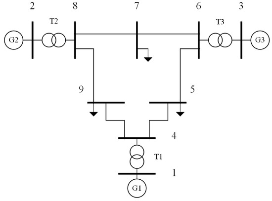
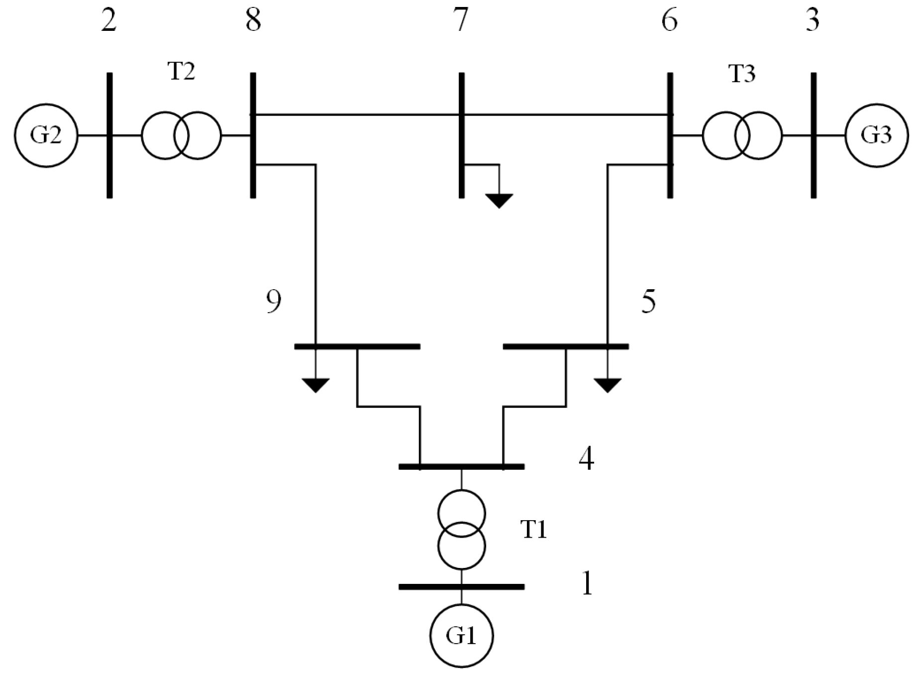
The IEEE 9-bus system shown in Figure 3 is used for the first case study. A 5% active-power imbalance is applied separately at Bus 6 and Bus 8, and the three methods are used to calculate the corresponding frequency-security indices. The inertia time constants of the synchronous generators at Buses 1, 2, and 3 are 9.5 s, 4.1 s, and 2.7 s, respectively.
Figure 3.
IEEE 9-bus system.
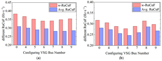
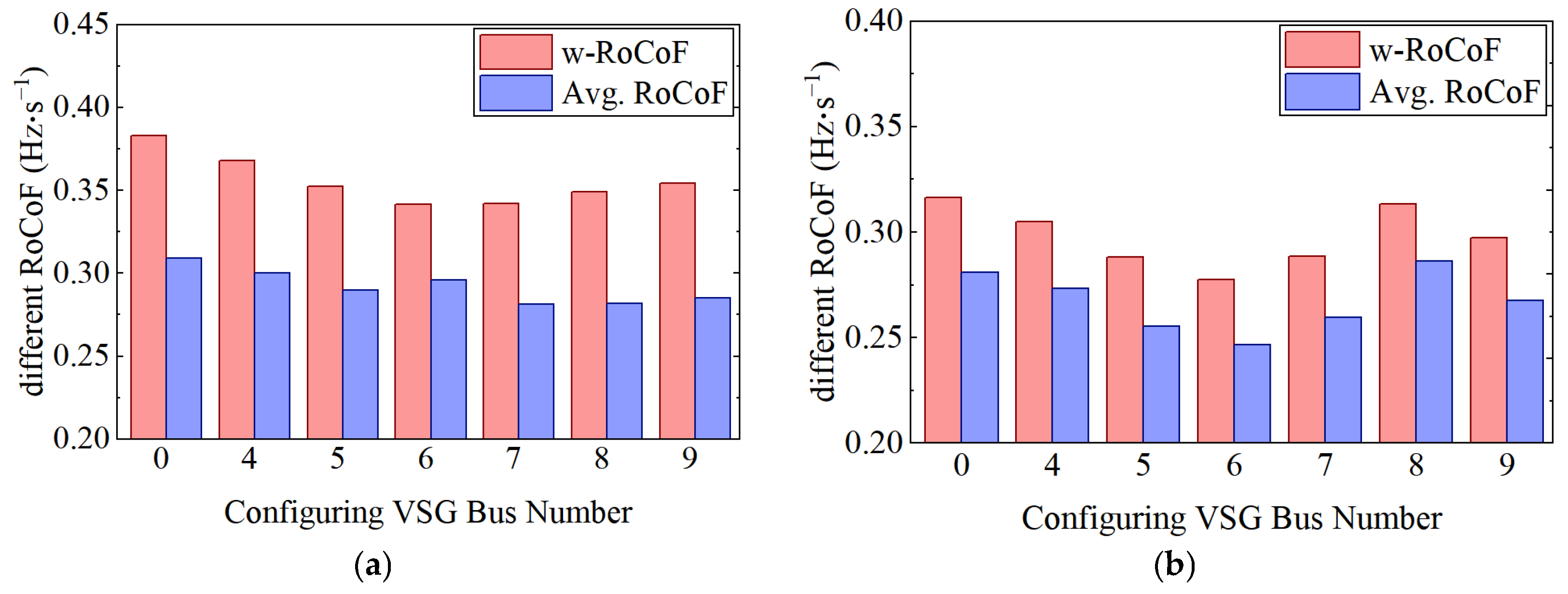
Figure 4 compares the values of the three assessment methods under different VSG placement buses when disturbances occur at different buses. The value 0 on the horizontal axis represents the case without VSG deployment. Since Buses 1, 2, and 3 are electrically close to Buses 4, 8, and 6, respectively, they are not discussed in this study; the same treatment is adopted in the following cases.
Figure 4.
Values of the three assessment methods under different VSG placement buses for different disturbance buses: (a) disturbance at Bus 8; (b) disturbance at Bus 6.
First, when the disturbance occurs at Bus 8, the values of the assessment methods under different VSG placement buses are observed. Both w-RoCoF and average RoCoF indicate that deploying the VSG at Bus 6 is the best choice. As shown in Figure 4b, when the disturbance occurs at Bus 6, the w-RoCoF result indicates that deploying the VSG at Bus 6 is optimal, whereas the average RoCoF result indicates that deploying the VSG at Bus 7 is optimal. Therefore, the values of these two indices vary when the VSG placement location and the disturbance location change.
According to Equation (1), the COI-based RoCoF is 0.2117 Hz/s before VSG deployment and 0.1856 Hz/s after VSG deployment, regardless of where the VSG is placed or where the disturbance occurs. This directly verifies the core assumption of COI theory discussed in Section 2: the system is equivalently represented as a single lumped-inertia system, and the frequency change rate is assumed to remain constant regardless of where the disturbance occurs. Therefore, the influence of the disturbance location on local frequency dynamics is completely ignored.
The bar charts in Figure 4 also show that the w-RoCoF values are generally larger than the average RoCoF values. This indicates that w-RoCoF can more sensitively capture the frequency dynamic behavior of critical generator buses. In contrast, the average RoCoF values under different placement buses vary only slightly, indicating that average RoCoF has limitations in reflecting the spatial characteristics of frequency dynamics and tends to produce relatively optimistic results.
The detailed maximum frequency deviation of each bus under different VSG placement schemes is reported in Table A1 of Appendix B. The tabulated results further verify the consistency between the ranking obtained by the proposed w-RoCoF index and the maximum-frequency-deviation results obtained from time-domain simulations.
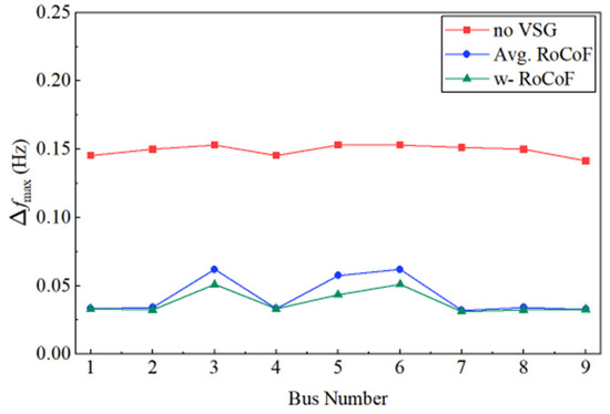
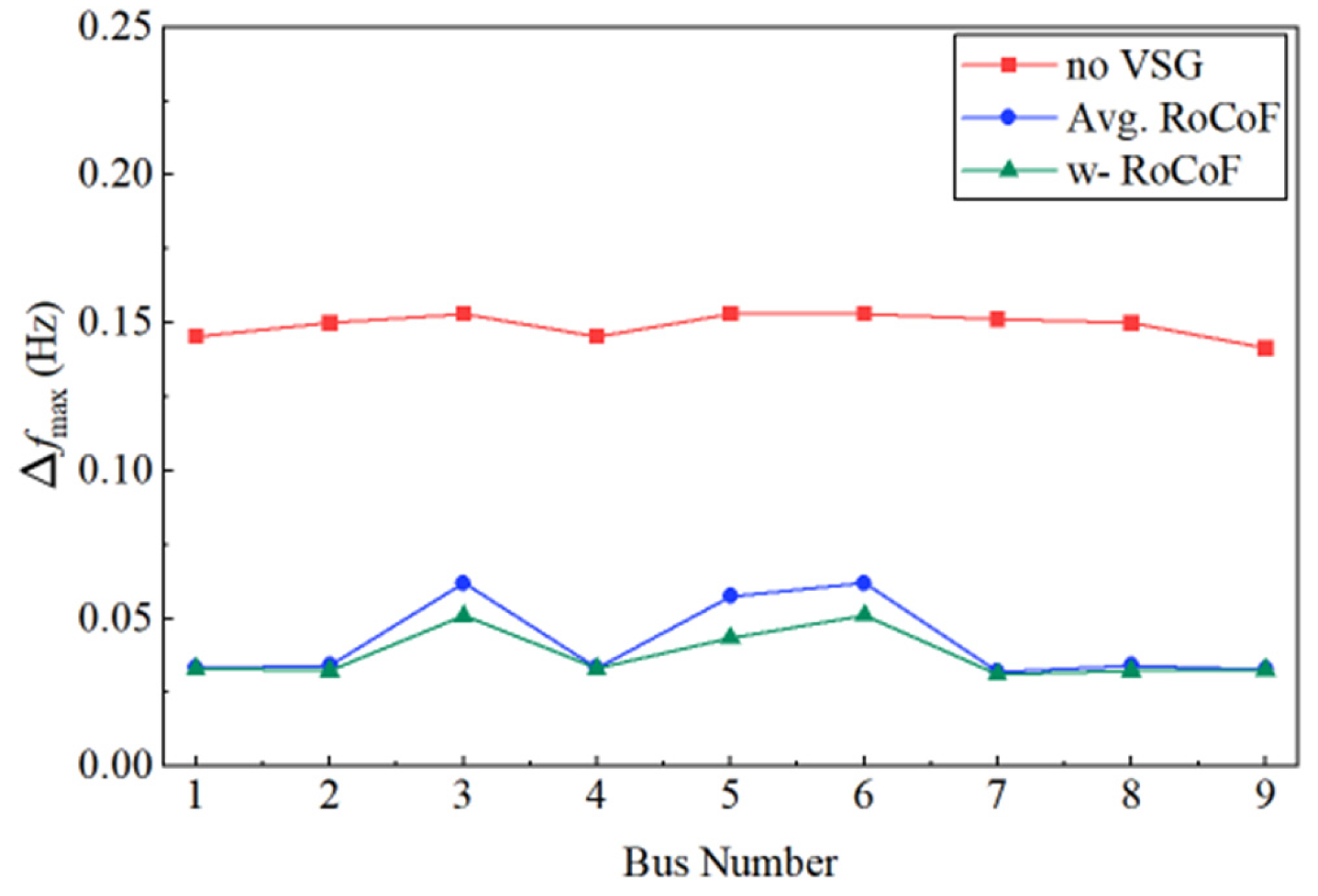
Based on Figure 4b, the configuration schemes selected by I2 and I3 are further simulated in PSCAD 5.0, and the maximum frequency deviation at each bus is calculated. The I3-based result selects Bus 6 as the optimal VSG placement bus, whereas the I2-based result selects Bus 7. As shown in Figure 5, after VSG deployment, both configuration schemes reduce the maximum frequency deviation at the buses after the disturbance. In particular, when the VSG is deployed at Bus 6 according to the I3 result, the maximum frequency deviations at most buses are smaller than those obtained when the VSG is deployed at Bus 7 according to the I2 result.
Figure 5.
Maximum frequency deviation at each bus after VSG placement using different methods under a disturbance at Bus 6.
Table 1 presents the detailed RoCoF values at each bus, which are calculated using frequency-divider theory. These values can be quickly verified by comparing the corresponding equations in the preceding derivation. It can be observed that the RoCoF at the VSG placement bus generally increases compared with that before configuration. This is because these buses are non-source buses before VSG deployment, and their RoCoF is determined by the inertia of the source buses and the system disturbance. After VSG deployment, these buses are converted into source buses, and their RoCoF is directly determined by their own inertia and the allocated disturbance power. If the allocated disturbance power is large while the configured inertia is relatively small, the VSG may be insufficient to effectively buffer the disturbance, causing the RoCoF to increase after configuration.
Table 1.
Nodal RoCoF values after VSG placement using different methods under a disturbance at Bus 6.
The above case study shows that the proposed w-RoCoF method has significant advantages in system frequency-stability assessment. It avoids the limitations of COI theory and the masking effect of average RoCoF on local frequency differences, thereby demonstrating the effectiveness of the proposed w-RoCoF index.
5.2. Validation of the Proposed Index and VSG Siting Analysis Under Different Renewable-Energy Penetration Levels
Grid-following wind turbines are added to the IEEE 9-bus system shown in Figure 3. Specifically, wind turbines are connected to Buses 1, 2, and 3, and their capacities are given in Table A2 of Appendix B. The total generation capacity of the system is kept unchanged, while the capacities of synchronous generators and wind turbines are adjusted so that the wind-power capacity accounts for 30% and 70% of the total generation capacity, respectively. This setting is used to simulate low-inertia systems. A disturbance is applied at Bus 8 in the modified 9-bus system. Similarly, the w-RoCoF and average RoCoF values are calculated when the VSG is deployed at different buses. The results are shown in Table 2 and Table 3.
Table 2.
RoCoF index values under different VSG placement buses with 30% renewable-energy penetration.
Table 3.
RoCoF index values under different VSG placement buses with 70% renewable-energy penetration.
5.2.1. Siting Analysis
When the renewable-energy penetration level is 30%, the w-RoCoF index selects Bus 7, whereas the corrected average RoCoF index selects Bus 6. The average RoCoF values at Buses 6 and 7 are very close, indicating weak discrimination between these two candidates. In contrast, w-RoCoF provides a clearer siting preference by assigning higher weights to buses with more severe pre-deployment frequency dynamics. When the penetration level increases to 70%, I3 selects Bus 6, whereas I2 selects Bus 5. Although the disturbance occurs at Bus 8, neither method necessarily selects the disturbance bus, indicating that VSG siting should depend on system parameters rather than only on disturbance location. Overall, the I3 results tend to point to inertia-weak areas, and the reduced post-deployment index values confirm the effectiveness of VSGs in improving frequency stability.
5.2.2. Maximum Frequency Deviation
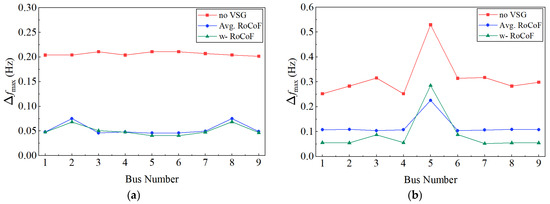
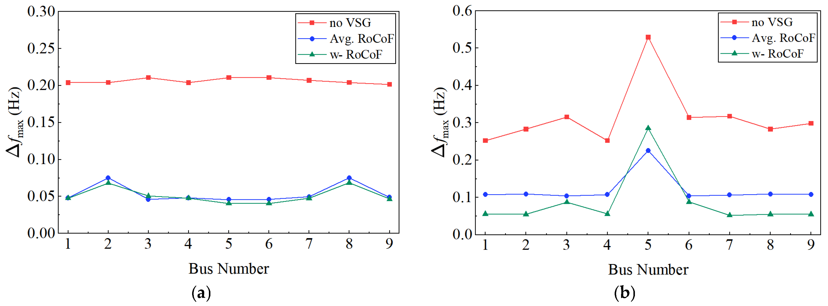
As shown in Figure 6, the configuration schemes in Table 2 and Table 3 are simulated, and the maximum frequency deviation at each bus is calculated. When the renewable-energy penetration level is 30%, the maximum frequency deviations under the I3-based configuration scheme are generally smaller than those under the I2-based scheme, except that the values at Buses 3 and 5 are slightly larger. When the renewable-energy penetration level is 70%, the simulation results show that, without VSG deployment, all buses experience severe frequency oscillations after a 5% active-power disturbance, and the system cannot reach a stable state for a long period after the disturbance. After VSG deployment, the frequency stability of both schemes is improved. Among them, the configuration scheme selected by I3 significantly reduces the nodal maximum frequency deviations, and the reduction is larger than that obtained using I2. This indicates that, in power systems with high renewable-energy penetration, the frequency-support effect of VSGs becomes more pronounced, highlighting the importance of VSGs in maintaining frequency stability under high renewable-energy integration. Meanwhile, the maximum-frequency-deviation results further verify the effectiveness of the I3 method.
Figure 6.
Maximum frequency deviation at each bus after VSG placement under different renewable-energy penetration levels: (a) 30% renewable-energy penetration; (b) 70% renewable-energy penetration.
5.3. VSG Optimal Configuration in the IEEE 39-Bus System with Renewable Energy Integration
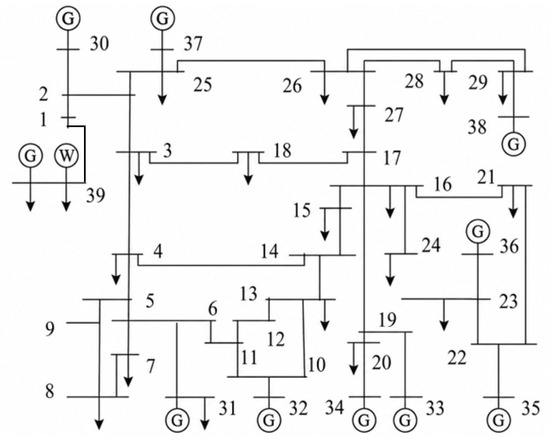
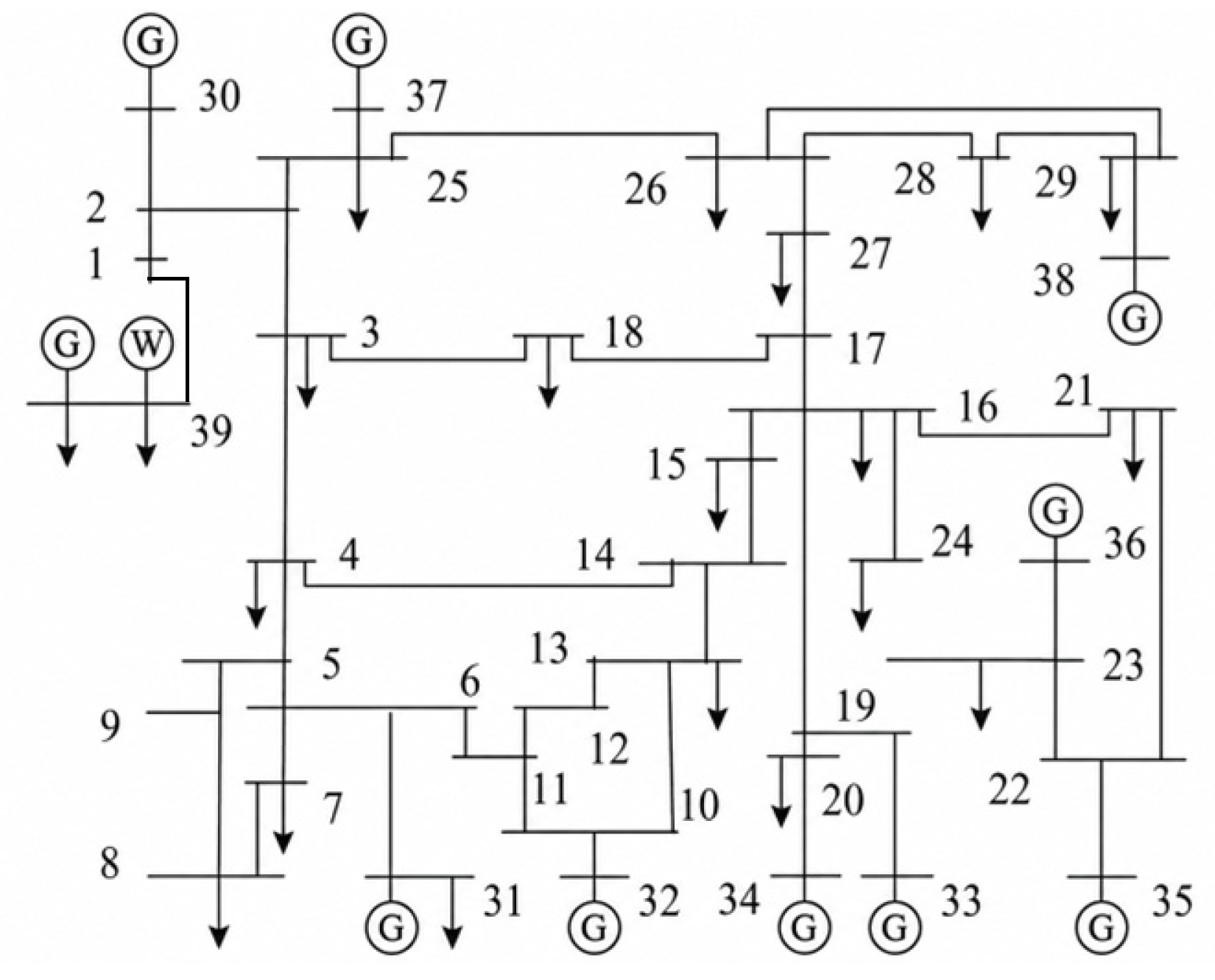
To simulate a low-inertia scenario with high renewable-energy integration at multiple buses, the large-capacity synchronous generator at bus 39 in the IEEE 39-bus system is replaced by a combined unit consisting of a synchronous generator and an equivalent wind-power generation unit, while the total generation capacity remains unchanged. After this modification, the equivalent system inertia is significantly reduced, and the inertia resources become spatially non-uniform. The structure of the modified IEEE 39-bus system is shown in Figure 7.
Figure 7.
Modified IEEE 39-bus system.
5.3.1. Index Effectiveness Analysis
Two disturbance scenarios are considered. In Case 1 (C1), a 5% active-power imbalance relative to the total system load is applied at Buses 15 and 16, which are located near the load center of the low-inertia area. In Case 2 (C2), on the basis of C1, an additional 5% active-power imbalance relative to the total system load is applied at Buses 21 and 24. Each VSG group is assumed to consist of ten VSG units. The virtual inertia constant is allowed to vary from 2 to 13 s, the total capacity is set to 100 MW, and the maximum number of VSG groups is set to two. The population size of the optimization algorithm is set to 50, and the maximum number of iterations is set to 100. The average RoCoF and w-RoCoF are used as objective functions, respectively. Table 4 presents the VSG single-objective optimization results obtained when the two indices are separately used as objective functions.
Table 4.
Optimal VSG configuration results under different schemes.
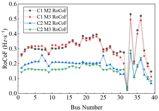
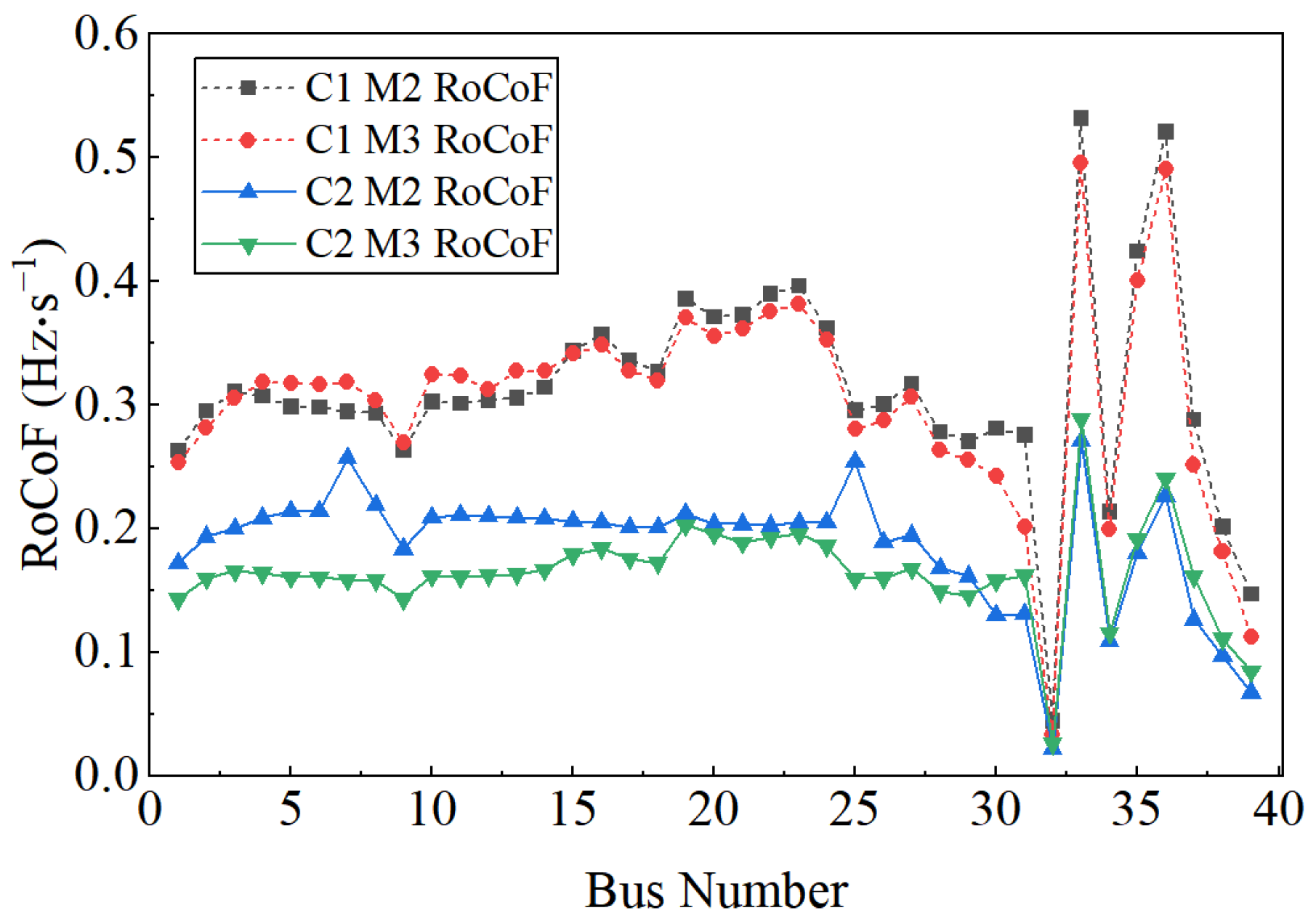
Table 4 shows that the optimal placement buses and virtual inertia values selected by the two methods are different. Method I3 selects buses close to generator buses, whereas Method I2 selects buses close to the disturbance locations. As shown in Figure 8, the four curves represent the nodal RoCoF values after VSG configuration using the two objective functions under the two disturbance scenarios. Although the I2 index reduces the average RoCoF level of the entire network, it does not effectively suppress the RoCoF peaks at critical weak buses, such as Buses 7 and 25 in C1. This indicates that the average value may mask local frequency risks.
Figure 8.
Nodal RoCoF values in the IEEE 39-bus system after VSG configuration using different methods.
For the w-RoCoF curves in C1 and C2, the proposed index reduces the average RoCoF level of the whole network and, more importantly, significantly suppresses the peak initial RoCoF values of several critical weak buses, such as Buses 15, 16, and 17. This is because the w-RoCoF index assigns higher weights to these buses in the objective function, causing the optimization process to preferentially improve their dynamic performance. These results demonstrate the superiority of w-RoCoF in the optimization model.
5.3.2. Comparison of Multi-Objective and Single-Objective Configuration Results
The C1 scenario is further used in this subsection to analyze the trade-off between frequency stability and configuration cost for VSG configuration. To implement multi-objective optimization, the boundaries of the objective functions must first be determined, namely, the ideal point and the worst point. The objective with w-RoCoF is denoted as F1, and the objective with virtual inertia is denoted as F2. The model is first solved using F1 and F2 as single objectives, respectively. The result obtained by solving F1 alone has been given above; therefore, the result obtained using F2 as the objective and the final multi-objective optimization result are calculated here.
Table 5 presents the results of the two single-objective optimizations and the final multi-objective optimization. The conflict between the two objectives can be clearly observed. When only the frequency-stability objective F1 is optimized, the system w-RoCoF reaches its minimum value, but F2 is relatively high. This indicates that more virtual inertia is required to achieve the desired frequency-stability performance, which increases the required configured virtual inertia. When only F2 is optimized, the virtual inertia reaches its minimum value, but w-RoCoF increases by 54.5%, indicating that frequency stability is neglected in order to reduce the required configured virtual inertia.
Table 5.
Results of single-objective and multi-objective optimization.
To further show the trade-off between frequency stability and configuration cost, several representative non-dominated solutions under the C1 scenario are listed in Table 6. As the total configured virtual inertia increases, the w-RoCoF value decreases, but the improvement in F1 becomes smaller when F2 increases from 1070 MW·s to 1333 MW·s, indicating a decreasing marginal benefit of additional virtual inertia.
Table 6.
Representative Pareto solutions under the C1 scenario.
The proposed multi-objective model therefore provides a compromise solution between the two objectives. Compared with the configuration considering only the required virtual inertia, it reduces the w-RoCoF value by 50.7%. Compared with the frequency-stability-oriented configuration, it reduces the required virtual inertia by 19.7%. These results demonstrate that the proposed model can improve frequency dynamic performance while limiting the required configuration scale.
5.3.3. Contingency-Set-Based Robust Planning Analysis
The deterministic cases above show that the optimal VSG placement may change when the disturbance location changes. To further improve the planning applicability of the proposed method, a contingency-set-based analysis is added in this subsection. The contingency set is designed to include representative disturbance locations in the low-inertia area, different disturbance combinations, and different renewable-energy penetration levels. The same VSG siting and sizing scheme is required to be evaluated under all scenarios in the set.
For each candidate VSG configuration, the w-RoCoF value is calculated under all scenarios in Table 7. The objective function follows the contingency-set extension described in Section 4.2, where both the weighted average performance and the worst-case performance are considered. The deterministic C1 and C2 optimization results are retained as benchmarks to show the limitation of optimizing against only one or two assumed disturbances.
Table 7.
Contingency set used for robust VSG planning.
As shown in Table 8, the deterministic schemes optimized for C1 or C2 perform well under their corresponding scenarios, but their worst-case w-RoCoF values increase when the disturbance location or renewable-energy penetration level changes. In particular, the deterministic C1 scheme still has three scenarios in which at least one nodal RoCoF constraint is violated. This confirms that the best VSG placement depends on the contingency location, and a configuration optimized for a limited number of disturbances may provide insufficient guidance for planning.
Table 8.
Comparison between deterministic optimization and contingency-set-based optimization.
In contrast, the proposed contingency-set-based I3 optimization selects Buses 8 and 25. This result is not identical to the optimal solution of any single deterministic scenario, but represents a compromise among multiple credible contingencies. All considered contingency scenarios satisfy the nodal RoCoF constraint. Compared with the I2-based contingency-set optimization, the proposed I3 method achieves a lower worst-case w-RoCoF, which indicates that the weighted index can better suppress frequency risks at critical buses instead of only reducing the whole-network average value.
To further check whether the RoCoF-oriented planning result is consistent with time-domain frequency-security performance, representative PSCAD simulations are carried out for the worst contingency of each configuration. The comparison is shown in Table 9.
Table 9.
Time-domain verification under the worst contingency of each configuration.
The time-domain results show that the contingency-set-based I3 scheme also achieves the smallest maximum frequency deviation, the highest frequency nadir, and the shortest settling time among the compared schemes. Therefore, although the proposed optimization model uses w-RoCoF as the main planning index, the obtained configuration also improves other important frequency-security indicators. This verifies the effectiveness of the proposed index and demonstrates that the contingency-set-based extension provides more practical planning guidance than the deterministic formulation.
Table A3 reports the computation times for index evaluation and one optimization run. The w-RoCoF index is evaluated rapidly because it is calculated analytically from disturbance-power allocation and the frequency-divider relationship. Although the optimization time increases with system size and the number of contingency scenarios, it remains acceptable for offline planning applications in the tested benchmark systems.
6. Conclusions
This paper investigated the VSG siting and sizing problem for frequency stability in renewable-energy-integrated power systems. The main conclusions are as follows.
First, compared with the COI-based and average nodal RoCoF indices, the proposed w-RoCoF index better captures spatial differences in nodal frequency dynamics. By assigning higher weights to frequency-vulnerable buses, it provides clearer siting guidance and avoids the masking effect of system-level averaging.
Second, the proposed multi-objective configuration model can balance frequency-security improvement and configuration economy. The Pareto results show an evident trade-off between w-RoCoF reduction and required virtual inertia, and the selected compromise solution improves frequency dynamic performance while limiting the required configuration scale.
Third, the optimal VSG placement is not necessarily located at the disturbance bus, but is closely related to inertia distribution, network topology, and disturbance location. The contingency-set-based results further show that the proposed method can provide more robust planning guidance under different disturbance locations and renewable-energy penetration levels. Time-domain simulations verify that the obtained configurations reduce maximum frequency deviation, improve frequency nadir, and shorten settling time.
At present, this study mainly focuses on the contribution of the inertial response capability of VSGs to the initial RoCoF and frequency stability. Practical factors such as communication delays, measurement errors, converter current limits, and renewable-generation uncertainties are not explicitly modeled in the current planning formulation. Future work will further incorporate these factors, together with the frequency-regulation capability of converter-interfaced power sources, into a more detailed VSG planning framework for practical power systems.
Author Contributions
Methodology, H.Y.; Formal analysis, H.Y.; Data curation, H.Y.; Writing—original draft, H.Y. and J.H.; Writing—review and editing, Z.W., H.D. and L.H. All authors have read and agreed to the published version of the manuscript.
Funding
This work is supported by Smart Grid-National Science and Technology Major Project (2025ZD0807200).
Data Availability Statement
The original contributions presented in this study are included in the article. Further inquiries can be directed to the corresponding author.
Conflicts of Interest
Author Liujun Hu and Hong Dong were employed by the company Guangzhou Power Supply Bureau, Guangdong Power Grid Co., Ltd. The remaining authors declare that the research was conducted in the absence of any commercial or financial relationships that could be construed as a potential conflict of interest.
Abbreviations
The following abbreviations are used in this manuscript:
| COI | Center of inertia |
| FD | Frequency divider |
| IBR | Inverter-based resource |
| IEEE | Institute of Electrical and Electronics Engineers |
| PFR | Primary frequency regulation |
| PSCAD | Power Systems Computer Aided Design |
| RoCoF | Rate of change of frequency |
| VSG | Virtual synchronous generator |
| w-RoCoF | Weighted rate of change of frequency |
| DC | Direct current |
Appendix A
Derivation of the Compromise-Based Multi-Objective Transformation.
Consider a multi-objective optimization problem with two conflicting objective functions, F1(x) and F2(x). When the two objectives are solved separately, their optimal solutions can be expressed as
Accordingly, the ideal point U and the worst point W in the solution space can be obtained as
To avoid dimensional inconsistency, the normalized distance of a solution point to the ideal point or the worst point along each objective direction can be expressed as
After normalization, the ideal point becomes (0,0), and the worst point becomes (1,1). The following distances are then defined:
where d+ denotes the distance from the solution point to the ideal point, and d- denotes the distance from the solution point to the worst point. f1 and f2 denote the normalized distances of the solution point to the ideal point along the F1(x) and F2(x) directions, respectively.
Thus, solving the multi-objective optimization problem can be transformed into minimizing the difference between the distance to the ideal point and the distance to the worst point, namely,
Furthermore,
Therefore, when the solution point is closest to the ideal point, the optimal solution of the multi-objective problem is obtained. In this way, the multi-objective optimization problem is transformed into a single-objective optimization problem.
Appendix B
Table A1.
Maximum nodal frequency deviation under different VSG placement buses when the disturbance occurs at Bus 6.
Table A2.
Capacity settings of synchronous generators and wind turbines under different renewable-energy penetration levels.
Table A3.
Computation times for index evaluation and one optimization run.
References
- Zhang, Z.; Zhang, N.; Du, E.; Kang, C.; Wang, Z. Review and Countermeasures on Frequency Security Issues of Power Systems with High Shares of Renewables and Power Electronics. Proc. CSEE 2022, 42, 1–24. [Google Scholar] [CrossRef]
- Mo, W.; Lei, J.; Chen, Y.; Chen, H.; He, J. Frequency Stability Challenges and Countermeasures in Typical Isolated Synchronous Power Grids with High Penetration of Renewable Energy, Part I. Power Syst. Prot. Control 2025, 53, 177–187. [Google Scholar] [CrossRef]
- Mo, W.; Ye, K.; Chen, Y.; Chen, H.; He, J. Frequency Stability Challenges and Countermeasures in Typical Isolated Synchronous Power Grids with High Penetration of Renewable Energy, Part II. Power Syst. Prot. Control 2025, 53, 178–187. [Google Scholar] [CrossRef]
- Zhang, W.; Wen, Y.; Chi, F.; Wang, K.; Li, L. Research Framework and Prospect on Power System Inertia Estimation. Proc. CSEE 2021, 41, 6842–6856. [Google Scholar] [CrossRef]
- Wang, B.; Yang, D.; Cai, G. Review of Research on Power System Inertia-Related Issues in the Context of High Penetration of Renewable Power Generation. Power Syst. Technol. 2020, 44, 2998–3007. [Google Scholar] [CrossRef]
- Leon, A.E.; Mauricio, J.M. Virtual Synchronous Generator Design to Improve Frequency Support of Converter-Interfaced Systems. IEEE Trans. Energy Convers. 2023, 39, 862–871. [Google Scholar] [CrossRef] [Scilit]
- Zhu, H.; Li, H.; Liu, G.; Ge, Y.; Shi, J.; Li, H.; Zhang, N. Energy Storage in High Variable Renewable Energy Penetration Power Systems: Technologies and Applications. CSEE J. Power Energy Syst. 2020, 9, 2099–2108. [Google Scholar] [CrossRef] [Scilit]
- Ajami, O.M.T.; Tan, R.H.G.; Nadarajah, M.; Jamaludin, F.A.; Pradana, A.B. Multi-Objective Optimization of HESS Control for Optimal Frequency Regulation in a Power System with RE Penetration. e-Prime—Adv. Electr. Eng. Electron. Energy 2024, 10, 100805. [Google Scholar] [CrossRef] [Scilit]
- Saha, S.; Elliott, M.; Roy, T.K.; Oo, A.M.T. Reliability-Constrained Optimization of Virtual Inertia and Battery Energy Storage System Sizing for Frequency Stability in Low-Inertia Power Systems. Sustain. Energy Grids Netw. 2026, 45, 102130. [Google Scholar] [CrossRef] [Scilit]
- Zhang, D.; Shafiullah, G.M.; Das, C.K.; Wong, K.W. Optimal Allocation of Battery Energy Storage Systems to Improve System Reliability and Voltage and Frequency Stability in Weak Grids. Appl. Energy 2025, 377, 124541. [Google Scholar] [CrossRef] [Scilit]
- Ramos, A.F.; Ahmad, I.; Habibi, D.; Mahmoud, T.S. Placement and Sizing of Utility-Scale Battery Energy Storage Systems to Improve the Stability of Weak Grids. Int. J. Electr. Power Energy Syst. 2023, 144, 108427. [Google Scholar] [CrossRef] [Scilit]
- Zhang, Y.; Kou, P.; Zhang, Z.; Tian, R.; Yan, Y.; Liang, D. Optimal Sizing and Siting of BESS in High-Wind-Penetrated Power Systems: A Strategy Considering Frequency and Voltage Control. IEEE Trans. Sustain. Energy 2023, 15, 642–657. [Google Scholar] [CrossRef] [Scilit]
- Li, J.; Huang, Y.; Dou, X.; Wang, S.; Chu, T. Optimal Energy Storage Configuration for Primary Frequency Regulation Performance Considering State-of-Charge Partitioning. IEEE Trans. Sustain. Energy 2025, 16, 2659–2668. [Google Scholar] [CrossRef] [Scilit]
- Li, Y.; Wen, Y.; Ye, X.; Jiang, X.; Lin, X. Estimation Method of Power System Nodal Inertia Based on Multi-Innovation Identification. Electr. Power Autom. Equip. 2022, 42, 89–95. [Google Scholar] [CrossRef]
- Liu, F.; Xu, G.; Liu, J.; Wang, C.; Bi, T.; Guo, X. Inertia Distribution Characteristics of Power System Considering Structure and Parameters of Power Grid. Autom. Electr. Power Syst. 2021, 45, 60–67. [Google Scholar] [CrossRef]
- Chen, J.; Hong, L.; Zheng, Z. Research and Application Development of Under-Frequency Load Shedding in Power Systems. Power Syst. Prot. Control 2007, 35, 79–82. [Google Scholar] [CrossRef]
- Basso, T.S.; DeBlasio, R. IEEE 1547 Series of Standards: Interconnection Issues. IEEE Trans. Power Electron. 2004, 19, 1159–1162. [Google Scholar] [CrossRef] [Scilit]
- GB/T 40596-2021; Technical Rules for Automatic Under-Frequency Load Shedding in Electric Power Systems. Standards Press of China: Beijing, China, 2021.
- Kundur, P. Power System Stability and Control; McGraw-Hill: New York, NY, USA, 1994. [Google Scholar]
- Golpîra, H.; Atarodi, A.; Amini, S.; Messina, A.R.; François, B.; Bevrani, H. Optimal Energy Storage System-Based Virtual Inertia Placement: A Frequency Stability Point of View. IEEE Trans. Power Syst. 2020, 35, 4824–4835. [Google Scholar] [CrossRef] [Scilit]
- Xu, D.; Wu, Z.; Guan, L. Distributionally Robust Optimal Configuration of Battery Energy Storage System Considering Nodal RoCoF Security Constraints. J. Energy Storage 2024, 104, 114707. [Google Scholar] [CrossRef] [Scilit]
- Milano, F.; Ortega, A. Frequency Divider. IEEE Trans. Power Syst. 2017, 32, 1493–1501. [Google Scholar] [CrossRef] [Scilit]
- Zhang, Q.; Li, X.; Lan, G.; Wang, X.; Shen, J.; Zeng, H.; Yuan, P.; Zhang, X.; Li, W. Analytical Frequency Security Indicators for Two-Region Interconnected Power Systems. IEEE Access 2024, 12, 107645–107655. [Google Scholar] [CrossRef] [Scilit]
- Shen, J.; Li, W.; Liu, L.; Jin, C.; Wen, K.; Wang, X. Frequency Response Model and Its Closed-Form Solution of Two-Machine Equivalent Power System. IEEE Trans. Power Syst. 2021, 36, 2162–2173. [Google Scholar] [CrossRef] [Scilit]
- Li, K.; Zhang, F.; Ding, L.; Sun, K.; Zhang, G.; Xin, Z. Differentiation Mechanism Analysis and Coordinated Control Methods for Multi-Area Frequency Deviation in Power Grids. Autom. Electr. Power Syst. 2026, 50, 77–89. [Google Scholar] [CrossRef]
- Liu, R.; Wang, Z.; Wu, J.; Zhao, T.; Shan, Y. Configuration Optimization of Virtual Inertia Considering Spatial Distribution Characteristics of Frequency. Autom. Electr. Power Syst. 2024, 48, 122–130. [Google Scholar] [CrossRef]
- Li, W.; Ding, Q. A Preliminary Research on the Representation Form of Spatiotemporal Distribution Characteristics of Power System Inertia under Large Disturbances. Proc. CSEE 2024, 44, 4601–4614. [Google Scholar] [CrossRef]
- Badesa, L.; Teng, F.; Strbac, G. Conditions for Regional Frequency Stability in Power System Scheduling—Part I: Theory. IEEE Trans. Power Syst. 2021, 36, 5558–5566. [Google Scholar] [CrossRef] [Scilit]
- Pérez-Illanes, F.; Álvarez-Miranda, E.; Rahmann, C.; Campos-Valdés, C. Robust Unit Commitment Including Frequency Stability Constraints. Energies 2016, 9, 957. [Google Scholar] [CrossRef] [Scilit]
- Anderson, P.M.; Fouad, A.A. Power System Control and Stability, 2nd ed.; IEEE Press: Piscataway, NJ, USA, 2003. [Google Scholar]
- Liu, J.; Wang, C.; Zhao, J.; Bi, T. RoCoF-Constrained Unit Commitment Considering Spatial Difference in Frequency Dynamics. IEEE Trans. Power Syst. 2023, 39, 1111–1125. [Google Scholar] [CrossRef] [Scilit]
- Badesa, L.; Teng, F.; Strbac, G. Optimal Portfolio of Distinct Frequency Response Services in Low-Inertia Systems. IEEE Trans. Power Syst. 2020, 35, 4459–4469. [Google Scholar] [CrossRef] [Scilit]
- Wu, Z.; Chen, C.; Xu, D.; Guan, L. Frequency-Constrained Economic Dispatch of Microgrids Considering Frequency Response Performance. Energies 2025, 18, 2014. [Google Scholar] [CrossRef] [Scilit]
- Mirjalili, S.; Mirjalili, S.M.; Lewis, A. Grey Wolf Optimizer. Adv. Eng. Softw. 2014, 69, 46–61. [Google Scholar] [CrossRef] [Scilit]

Disclaimer/Publisher’s Note: The statements, opinions and data contained in all publications are solely those of the individual author(s) and contributor(s) and not of MDPI and/or the editor(s). MDPI and/or the editor(s) disclaim responsibility for any injury to people or property resulting from any ideas, methods, instructions or products referred to in the content. |
© 2026 by the authors. Licensee MDPI, Basel, Switzerland. This article is an open access article distributed under the terms and conditions of the Creative Commons Attribution (CC BY) license.