GNN-Based Degradation Model Development for an NMC Li-Ion Battery

Abstract

Accurate state-of-health (SoH) prediction is vital for safe and efficient battery management, enabling extended lifespan and improving technologies such as electric vehicles and stationary energy storage systems. In this work, a graph neural network-based deep learning framework is proposed to predict the SoH of a commercial nickel–manganese–cobalt oxide (NMC) lithium-ion technology. Health indicators obtained from the in-house-generated experimental aging dataset are used to train and validate the model across batteries subjected to diverse operating conditions. The hybrid architecture combines graph neural networks (GraphSAGE) with convolutional neural networks (CNN) and long short-term memory (LSTM) blocks, capturing both local structural relationships and temporal patterns in the battery data. Evaluation results show strong predictive performance, achieving an R² of 0.989 and a mean squared error of 3.23 × 10⁻⁶. These findings suggest that the proposed methodology could be deployed as a useful diagnostic tool.

1. Introduction

The ongoing and increasing demand for electric vehicles (EVs), besides portable electronics, has underscored the essential role of lithium-ion batteries (LiBs) in modern technology [1]. LiBs are favored for their higher specific energy, longer cycle life, lower self-discharge, and mature manufacturing ecosystem, making them the dominant choice for applications that require reliable, high-performance energy storage [2,3]. Among the various chemistries available, nickel–manganese–cobalt oxide (NMC) cathodes have gained prominence. NMC offers a compelling balance of high energy density, good rate capability, and enhanced thermal stability compared with alternatives such as lithium cobalt oxide (LCO), lithium iron phosphate (LFP), or lithium nickel cobalt aluminum oxide (NCA) [4,5].

Despite their advantages, NMC-based cells remain susceptible to a variety of degradation mechanisms (such as loss of active material, electrolyte decomposition, and resistance growth) that gradually reduce capacity, increase internal resistance, and ultimately limit their service life [6,7]. Understanding and mitigating these degradation phenomena are critical for enhancing the longevity and effectiveness of NMC-based batteries in practical applications [8].

Accurate modeling of the degradation of NMC cells is therefore crucial for predicting lifetime and optimizing battery usage in critical applications. By combining knowledge of degradation pathways with advanced predictive models, it is possible to implement more effective battery management strategies, extend service life, and improve overall performance [9,10].

Approaches to battery health prediction can be broadly divided into physics-based models and data-driven methods. Semi-empirical and physics-based models use electrochemical principles to simulate degradation mechanisms. While interpretable, they require extensive parameterization and are computationally intensive, limiting their real-time applicability [11,12].

Data-driven methods (particularly neural networks) have become popular for capturing complex, nonlinear relationships directly from experimental data [13]. Recurrent neural networks (RNNs) and their variants, like long short-term memory (LSTM) networks, have been widely applied to capture long-term temporal dependencies in cycling data, as done by Xu et al. [14]. Convolutional neural networks (CNNs) perform well at extracting local patterns from voltage or current profiles, making them effective at identifying early signatures of degradation within individual cycles [14,15]. Hybrid CNN-LSTM models have already achieved high predictive accuracy for the state of health (SoH) and remaining useful life (RUL) estimation [16].

Graph neural networks (GNNs) have more recently been introduced to battery prognosis [17]. They can represent complex relational structures, such as correlations between health indicators, inter-cycle dependencies, or interactions among cells in a pack [18,19]. Studies have demonstrated that incorporating graph structures improves SoH estimation by modeling spatio-temporal degradation dynamics [20,21]. Combining GNNs with CNN and LSTM components allows local feature extraction (with CNN), long-term temporal modeling (with LSTM), and explicit relational reasoning (with GNN) within a unified framework, which can enhance robustness and generalization compared with using any single architecture alone.

This work presents a hybrid GNN–CNN–LSTM model for health-status prediction of a commercial NMC-based high-energy pouch format LiB. The novel contributions of the research work are:

• Detailed experimental study on commercial NMC cells with variable aging conditions. Raw voltage, current, temperature, and capacity measurements were cleaned, normalized, and synchronized to ensure data quality for model training.
• Quantitative health indicators (HIs) were represented as nodes in a graph, with edges encoding correlations or physically meaningful relationships between indicators or cycles. This includes capturing different aspects of battery aging extracted from the cycling data.
• The implementation of a graph-based model, incorporating LSTM and CNN architectures. This process involves the selection of network architectures and the configuration of model parameters to ensure optimal performance. Sixteen cells were allocated for training and validation, while one worldwide harmonized light vehicles test (WLTC)-cycled cell was reserved exclusively for testing to evaluate model generalization.

The remainder of the manuscript includes a description of the materials and methods in Section 2, Section 3 describes the results and HI analysis, model architecture details are in Section 4, validation and discussion in Section 5, and the conclusion and future work are provided in Section 6.

2. Materials and Methods

2.1. Cell and Cycler Details

The data used in this project were obtained from long-term aging tests over 2 years. These raw test files were analyzed to extract the information required for the aging model. Before delving into the analysis, the laboratory procedures used to perform the various tests on different battery cells will first be described.

The experimental setup employed in this study involves the investigation of 18 commercial pouch-format cells with the NMC/Graphite chemistry. The specification of the battery cell is detailed in Table 1. For confidentiality reasons, the exact composition of the cathode material remains undisclosed. The cells underwent a series of preconditioning, electrical, and environmental tests to ensure accurate and reliable data collection for modeling purposes.

Table 1. Studied cell specifications.

Cell Specification
Cell chemistry	NMC/C
Nominal capacity	≥40 Ah (41.0 ± 1.0 Ah)
Nominal voltage	3.7 V
Operating voltage range	3–4.2 V
DC internal resistance	≤0.6 mΩ
Dimensions	224 mm × 225 mm × 9.8 mm
Weight	920 g ± 5 g

The principal equipment used in the electrical test campaign included PEC (from Leuven, Belgium)-manufactured ACT0550 model battery cyclers and climate chambers manufactured by CTS (CTS Benelux, Aalst, Belgium) to control environmental conditions. The lifetime characterization includes three types of tests: cycle life, validation test, and intermediate characterization test. The check-up or monitoring tests are also performed at the beginning of life (BoL), during intermediate breaks, and at the end of life (EoL) to assess the state of health (SoH) of the cells. The SoH is measured in terms of capacity loss and internal resistance growth. The flowcharts of the aging tests that have been followed can be summarized as described in Table 2.

Table 2. Table of cell conditions.

Cell	DoD (%)	Middle SoC (%)	T (°C)	CHA C-Rate	DCH C-Rate
1	100	50	25	1C	1C
2	60	50	25	1C	1C
3	40	50	25	1C	1C
4	20	50	25	1C	1C
5	100	50	25	1C	2C
6	100	50	25	2C	1C
7	40	80	25	1C	1C
8	40	20	25	1C	1C
9	20	80	25	1C	1C
10	20	20	25	1C	1C
11	40	50	25	2C	1C
12	100	50	45	1C	1C
13	60	50	45	1C	1C
14	20	50	45	1C	1C
15	100	50	10	1C	1C
16	20	50	10	1C	1C

Preconditioning and Test Set-Up

• Cell Preconditioning: It includes a few charge–discharge cycles to activate ions within the electrochemical energy storage system and to confirm a robust electrical connection setup. A constant current constant voltage (CCCV) method is used for charging, while CC discharge is employed within the specified voltage range.
• Capacity Check-up: This test is conducted at cyclic temperature using several charge–discharge cycles at a C/2 rate. Here, C-rate refers to the nominal current. The first tested value is considered the BoL capacity, and the capacity loss (CL) is then calculated by dividing the actual discharged capacity by the BoL in each case.
• Hybrid Pulse Power Characterization (HPPC): The test is performed at three different SoC levels (80%, 50%, and 20%) and 10 s pulses of three C (Current)-rates (0.33C, 0.5C, and 1C) to determine the internal resistance. Similarly, the calculation of the resistance increase (RI) is made from the actual and BoL values, where the resistance determined with a discharge pulse of 1C at 80% SoC is considered for comparative purposes.

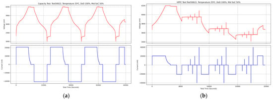
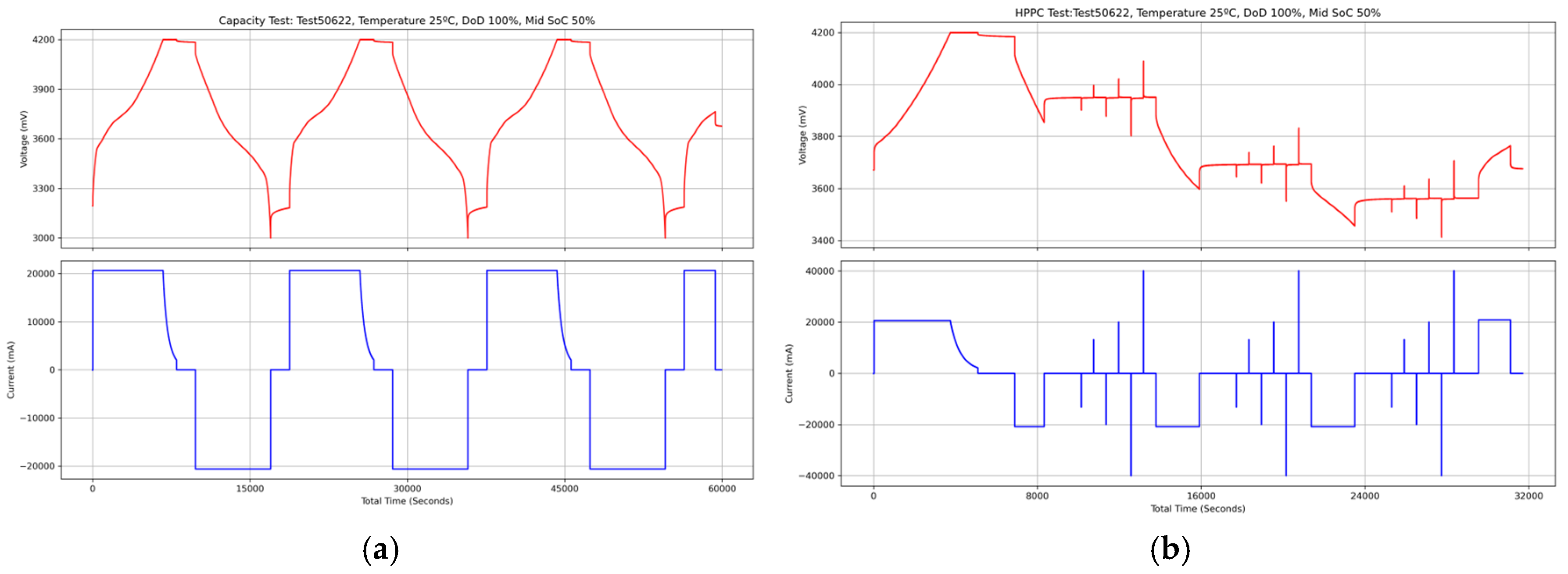
Regular checkups (capacity tests and HPPC, Figure 1) are conducted every 100 full equivalent cycles (FECs) initially, up to the seventh short checkup. An FEC is calculated based on charging the Ah throughput based on the rated capacity value. Subsequently, checkups are performed every 200 FECs until the seventeenth short checkup, and then every 300 FECs until the end of the testing period. This adjustment is due to the observation that significant degradation was not evident with more frequent evaluations.

Figure 1. (a) Capacity Test. Plot of the voltage and current versus time; (b) HPPC Test. Plot of the voltage and current versus time.

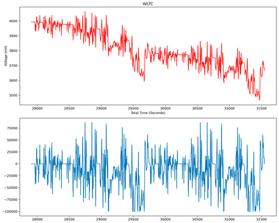
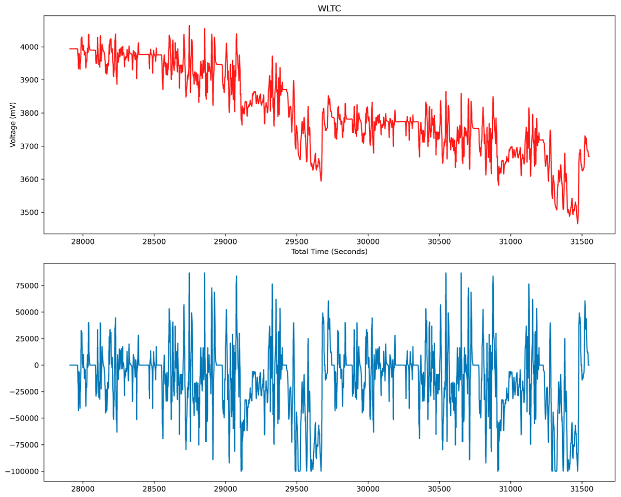
• Standard Validation Test: Emulating real-life driving behavior, a standard WLTC test cycle is calculated at the cell level and performed on separate cells. A one-hour-long WLTC test cycle, as shown in Figure 2, includes two suburban dynamic streams performed at 90% SoC and 25 °C. The rounds of continuous WLTC cycling were conducted for 12 days before verifying the capacity and internal resistance of the cells. An aggressive WLTC is chosen to accelerate the aging. A single WLTC cycle discharges the cell at 33% depth of discharge (DoD) (SoC window of 90%–57%) before fully charging to 90% again. For the test cells (17 and 18), the check-ups are conducted every 100 FECs for the duration of the entire process.
  

  Figure 2. A dynamic current and voltage profile obtained from a light-duty vehicle (WLTC) under a real-life usage condition (Cell 18).

The goal is to generate high-quality data by selecting appropriate intervals within the safe operating area. The cycle life matrix consists of five different cycling depths, three mid-SoC points, three temperature conditions, and two combinations of charge–discharge rates.

2.2. Health Indicators Extraction

A high-quality dataset was generated from the experimental work, where the time domain information was filtered from raw files. The file types were organized as per test type so that crucial features or indicators could be extracted efficiently. Health indicators provide a quantitative view of battery aging and degradation, allowing for predictions of remaining capacity and lifespan. In this study, two main types of tests have been utilized: capacity tests and high-precision pulse power characterization tests, in addition to the cycling conditions.

Capacity tests are fundamental for determining the actual capacity of the battery under different charge and discharge states. These tests provide essential data on how the battery’s capacity degrades over time and usage, which is a direct indicator of its SoH. On the other hand, HPPC tests allow for the evaluation of the internal resistance and its ability to deliver power in short bursts. These data are crucial for understanding the battery’s dynamics under variable load conditions and for identifying changes in internal resistance that may indicate degradation of the active material and electrolyte.

The parameters derived from these tests include factors that affect battery behavior. Table 3 lists the selected HIs.

Table 3. Four categories of HIs were extracted from the experimental dataset [17].

HI Type	#	HIs
Static	1	Cycling Temperature
	2	Discharge Capacity
	3	Charge Capacity
	4	Internal Resistance
	5	Depth of Discharge
	6	Middle State of Charge
	7	Discharge C-rate
	8	Charge C-rate
	9	Cycle Number
Variable (Current-related)	10	Area under Current Curves of CC Process
	11	Area under Current Curves of CV Process
	12	Area under Current Curves of CC-CV Process
	13	Area under Current Curves of Discharge Process
Variable (Voltage-related)	14	Area under Voltage Curves of CC Process
	15	Area under Voltage Curves of CV Process
	16	Area under Voltage Curves of Discharge Process
Variable (Time-related)	17	Discharge Time
	18	Charging Time
	19	CC Stage Period
	20	CV Stage Period

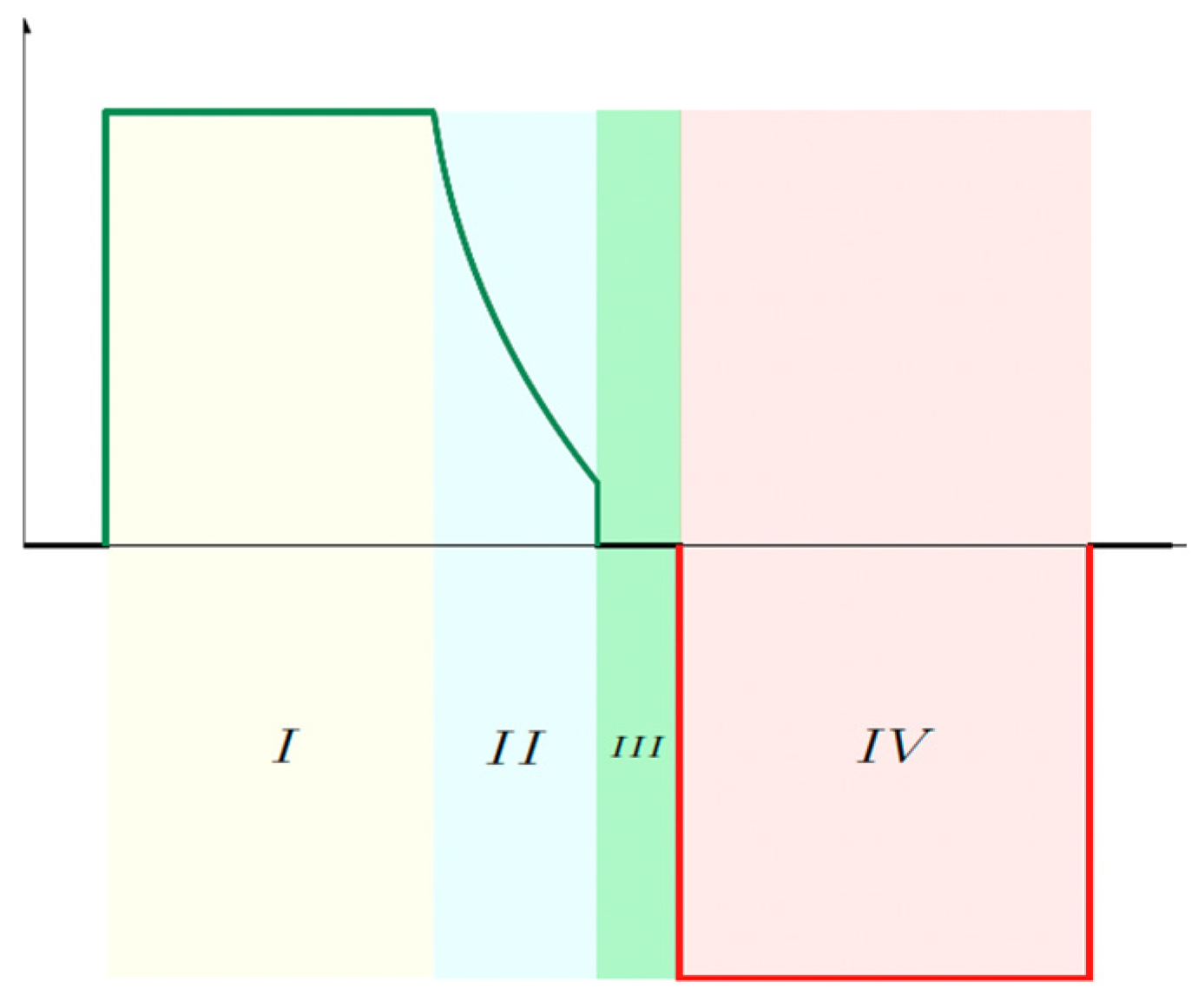
In this study, the HIs have been classified into two main categories: Static and Variable. Four areas in the Capacity test were defined, as shown in Figure 3:

Figure 3. Sample current curve from the capacity test (3rd cycle), HI extraction zones.

• I: CC charge–constant current during charge.
• II: CV charge–constant voltage during charge.
• III: Rest period.
• IV: CC discharge–constant current during discharge.

3. Results Analysis of Health Indicators

In this section, a comprehensive analysis of the health indicators calculated in the previous section is undertaken. The primary aim is to assess the influence of various HIs on the health state of NMC cells. This analysis is crucial for understanding how different operational parameters and degradation mechanisms impact battery performance over time. By examining the data, the HIs most indicative of battery health are identified, potential outliers are discerned, and the redundancy or relevance of each HI is determined.

A key metric in evaluating battery health is the state of health, which quantifies the remaining useful capacity relative to its initial capacity. Mathematically, SoH is expressed as:

$$SoH={\displaystyle \frac{Q_t}{Q_0}}\times 100\%$$

(1)

where Q_t is the actual discharge capacity, and Q₀ is the BoL discharge capacity. This formula provides a percentage that reflects the extent of capacity degradation over time, with 100% indicating a new battery and lower values corresponding to decreased performance due to aging and cycling.

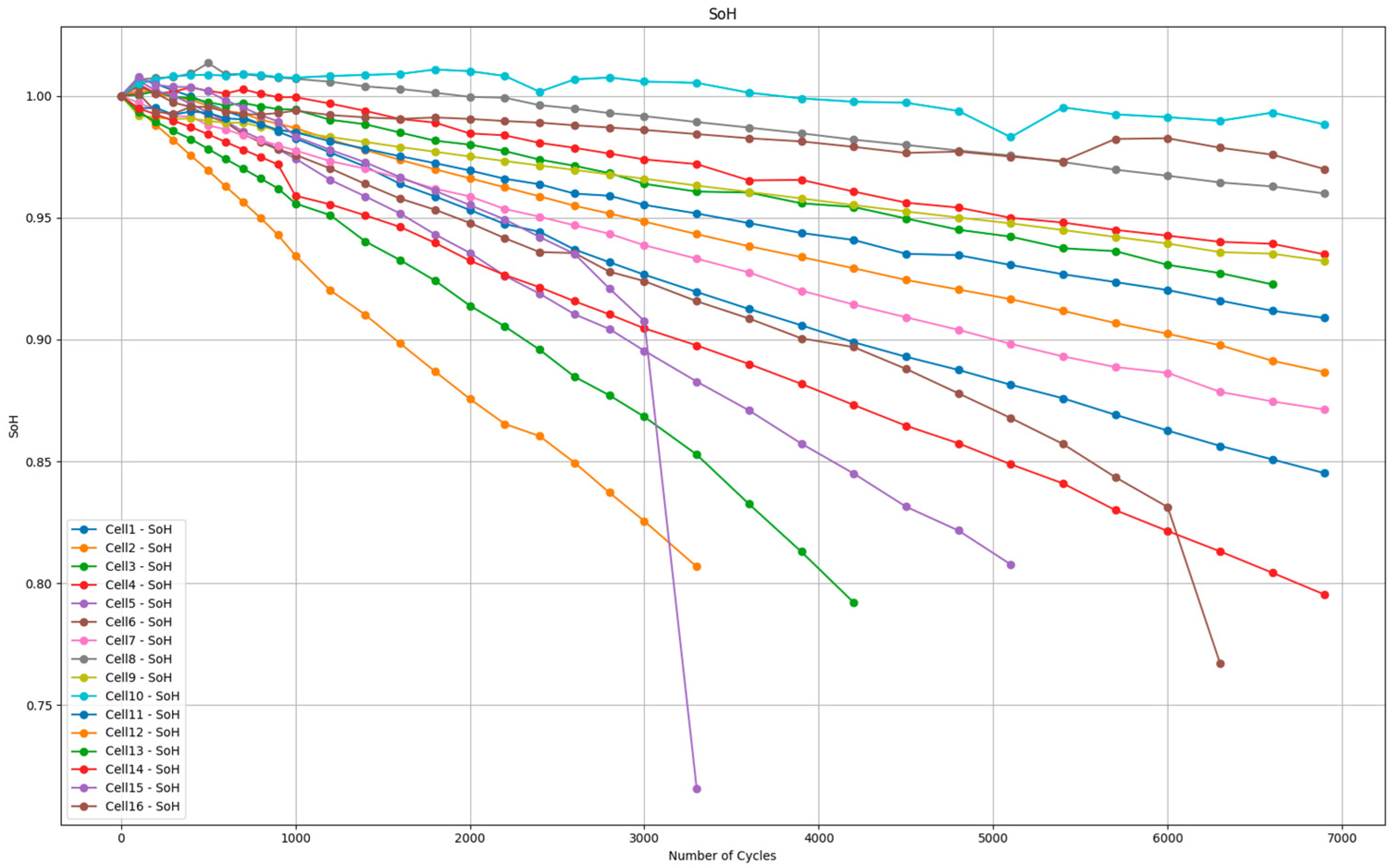
Figure 4 shows the SoH values of all the studied cells derived from the actual discharge capacity. For this analysis, it is essential to have in mind the table with the cell conditions.

Figure 4. SoH values of the 16 cells.

The first step that is taken in this analysis is the use of the Pearson correlation [22]. This correlation coefficient is a statistical measure that evaluates the linear relationship between two variables. It is denoted as ρ and ranges from −1 to 1, where:

$$\mathsf{\rho }={\displaystyle \frac{\sum \left(x_i-\overline{x}\right)\left(y_i-\overline{y}\right)}{\sqrt{\sum {\left(x_i-\overline{x}\right)}^2\sum {\left(y_i-\overline{y}\right)}^2}}}$$

(2)

where x_i and y_i are the individual sample points, and $\overline{x}$ and $\overline{y}$ are the means of the x and y variables, respectively. The Pearson correlation is widely used because it quantifies the degree to which two variables are linearly related, making it a useful tool for identifying and understanding relationships in data. The representation of the Pearson correlation values for every variable HI and for every cell is utilized to find the most suitable HIs as per the sensitivity threshold.

This first approach shows that the discharge capacity (HI2), charge capacity (HI3), area under CC charge current (HI10), and area under discharge current (HI12) are the most positively correlated HIs. Also, internal resistance (HI4), area under voltage curves of CV process (HI15), and CV stage period (HI20) are clear signs of high negative correlation, indicating that increasing these values corresponds to a deterioration of the cell’s health.

3.1. Influence of the Cell Conditioning

The Pearson correlation analysis is not suitable for examining factors that remain constant over time, such as the conditioning of the cells. To assess how these variables impact the cell’s health, a different approach is required. A more effective method involves selecting cells with identical conditions, varying only a single variable. By isolating this variable, its influence on the SoH can be analyzed by tracking its evolution over time. Four distinct parameters can be isolated for this analysis: temperature, DoD, middle SoC, and C-rate.

3.1.1. Temperature Impact

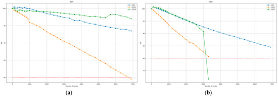
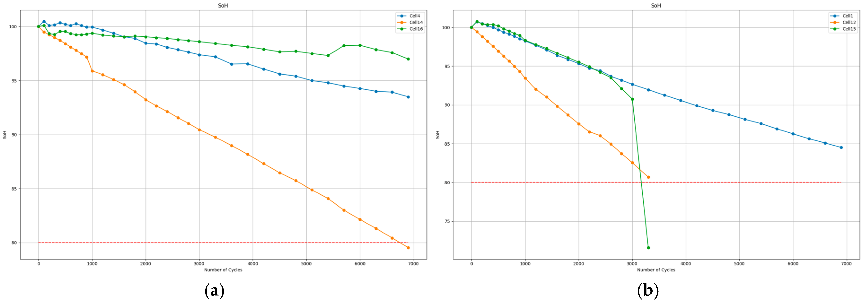
The experimental results are analyzed by comparing different conditions. Figure 5a clearly demonstrates that the higher temperature significantly impacts the cell’s SoH. The cell operating at 45 °C is the only one that reaches the EoL, indicating a capacity fade exceeding 20% relative to its initial capacity. In this scenario, with a low depth of discharge, the cell at 10 °C performs better than the cell at 25 °C. However, considering cells 1, 12, and 15, which are also at 25, 45, and 10 °C, respectively, but with a 100% DoD, Figure 5b shows that the cell at the lowest temperature experiences an abrupt decrease in capacity. Thus, temperature is a critical factor in battery capacity fade; both extremely high and extremely low temperatures accelerate degradation [23,24].

Figure 5. (a) SoH evolution with three cells that were operated in similar conditions except temperature: cell 4 at 25 °C, cell 14 at 45 °C, cell 16 at 10 °C; (b) SoH evolution with three cells that were operated in similar conditions except temperature: cell 1 at 25 °C, cell 12 at 45 °C, cell 15 at 10 °C. The red dashed line refers to the end of first limit of 80% SoH.

3.1.2. Middle SoC Impact

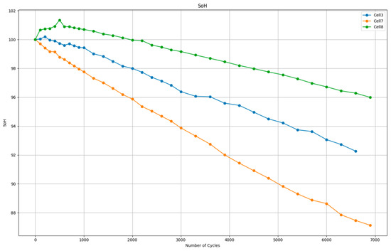
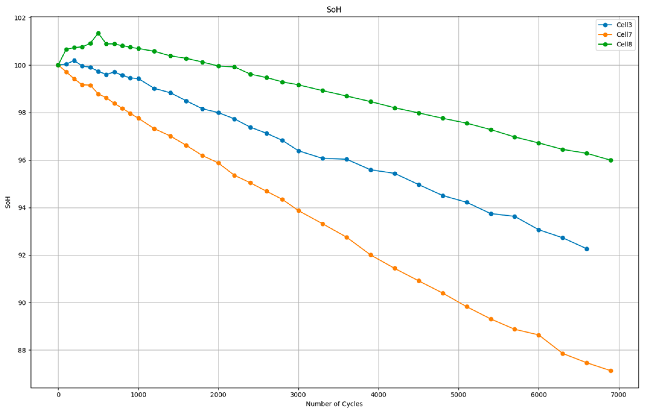
Similar analysis is done where cells were tested at 80%, 50%, and 20% middle SoC, respectively, at the same DoD, temperature, and C-rate. Figure 6 shows that the mid-SoC is also an important factor affecting the cell’s capacity. In this case, a higher mid-SoC leads to greater capacity fade. However, the impact on capacity is less pronounced than that of temperature.

Figure 6. Mid-SoC influence on the cell’s capacity for cells 3, 7, and 8.

3.1.3. DoD Impact

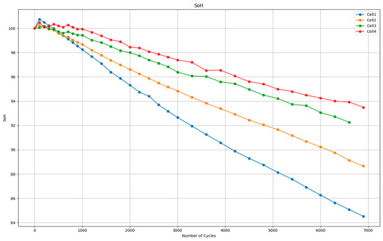
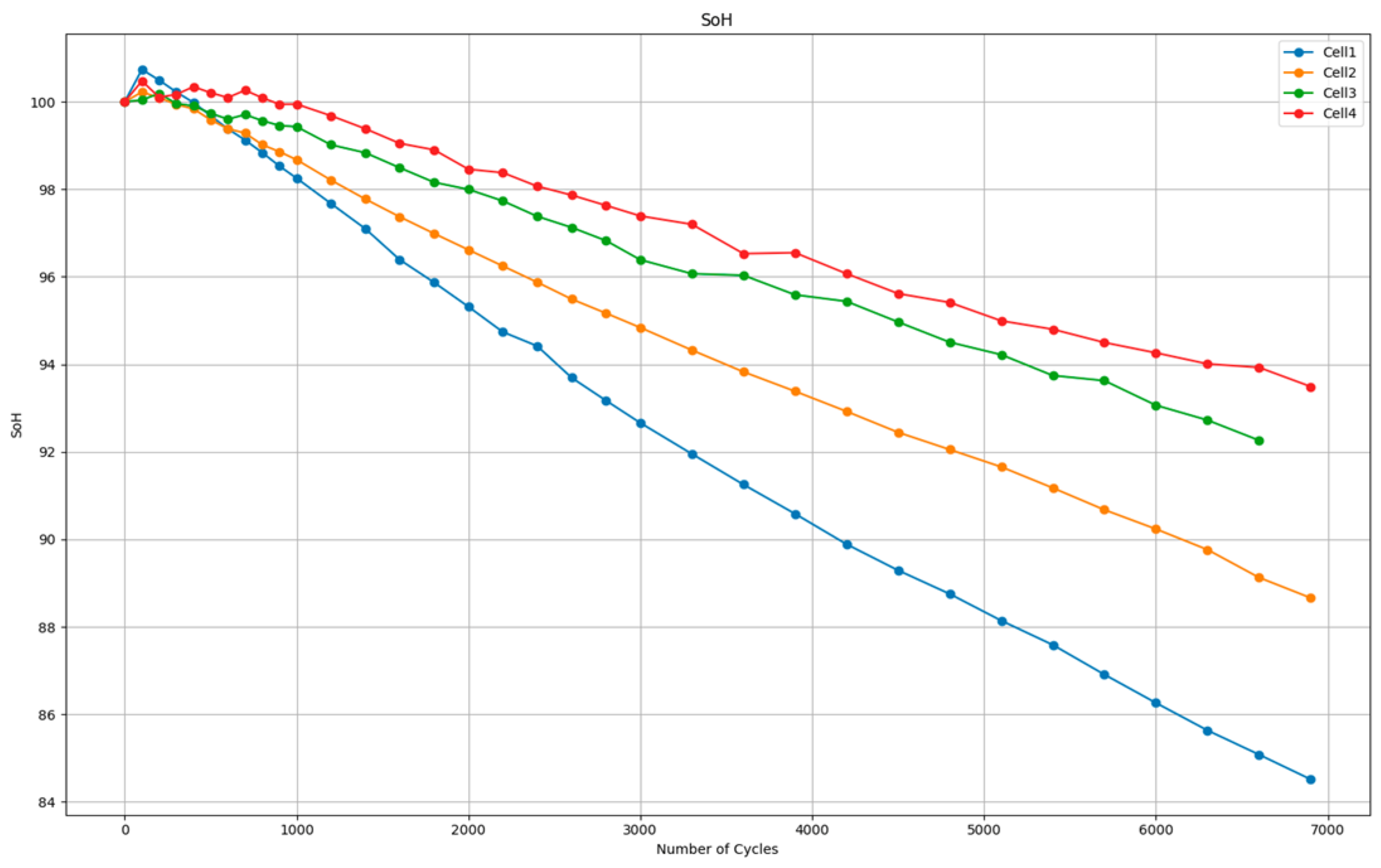
For the depth of discharge, as illustrated in Figure 7, cells cycled at higher DoD experience more pronounced capacity fade, highlighting the importance of including DoD as a factor in the model [25,26]. The displayed figure shows that higher DoD results in a higher SoH drop for four cells.

Figure 7. DoD impact on the cell’s capacity for cells 1, 2, 3, and 4.

3.1.4. C-Rate Impact

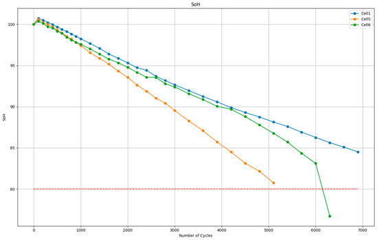
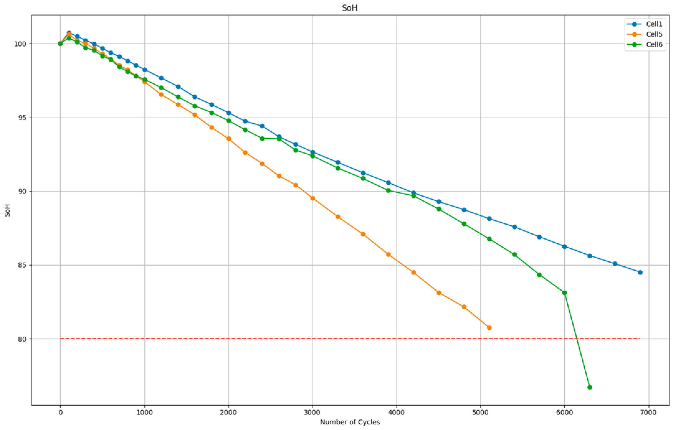
This C-rate variability is low in the experimental conditions due to the low number of cells. However, the corresponding SoH results for three cells are shown in Figure 8. A dependence of SoH on C-rates is observed: a higher discharge C-rate leads to increased capacity fade. For charging, although the initial slope is less steep, cell 6 exhibits an abrupt capacity drop in the final cycles. This confirms that higher C-rates accelerate cell degradation, which is a well-known observation in the literature [25,27].

Figure 8. C-rate influence on the cell’s capacity for cells 1, 5, and 6. The red dashed line refers to the end of first limit of 80% SoH.

3.2. HI Selection for Machine Learning Model

Feature selection was performed using three complementary criteria: correlation with SoH, redundancy between indicators, and physical relevance to battery degradation. The objective was to retain indicators that provide complementary information while avoiding unnecessary duplication and excessive model complexity.

For each time-varying indicator, the Pearson coefficient was calculated separately for every cell using the corresponding SoH sequence. The Pearson coefficient between variables $x$ and $y$ was calculated as

$$r_{x,y}={\displaystyle \frac{{\displaystyle {\sum }_{k=1}^n}\left(x_k-\overline{x}\right)\left(y_k-\overline{y}\right)}{\sqrt{{\displaystyle {\sum }_{k=1}^n}{\left(x_k-\overline{x}\right)}^2}\sqrt{{\displaystyle {\sum }_{k=1}^n}{\left(y_k-\overline{y}\right)}^2}}}$$

(3)

SoH for cell $c$ at check-up $k$ was calculated from the measured discharge capacity as

$${\mathrm{S}\mathrm{o}\mathrm{H}}_{c,k}={\displaystyle \frac{Q_{c,k}}{Q_{c,0}}}\times 100$$

(4)

where, $Q_{c,k}$ is the discharge capacity measured at check-up $k$ and $Q_{c,0}$ is the corresponding beginning-of-life capacity.

Since the sign of a correlation may differ between cells while the strength of the relationship remains high, both the mean signed coefficient and the mean absolute coefficient were considered. For indicator $j$, the mean absolute correlation was calculated as

$$\overline{\left|r_j\right|}={\displaystyle \frac{1}{N_c}}{\displaystyle {\sum }_{c=1}^{N_c}}\left|r_{j,c}\right|$$

(5)

where, $r_{j,c}$ is the correlation coefficient obtained for the indicator $j$ in cell $c$, and $N_c$ is the number of evaluated cells.

A correlation-based relevance contribution was then calculated as -

$$C{R}_j={\displaystyle \frac{\overline{\left|r_j\right|}}{{\displaystyle {\sum }_{m=1}^M}\overline{\left|r_m\right|}}}\times 100$$

(6)

where, $M$ represents the number of time-varying indicators included in the comparison. This percentage represents the relative statistical relevance of each indicator during the pre-model feature selection stage and should not be interpreted as a model-specific feature importance.

Temperature, DoD, middle SoC, charge C-rate, and discharge C-rate remain constant within the aging sequence of an individual cell. Consequently, their effects cannot be evaluated using within-cell Pearson correlation. Temperature, DoD, and middle SoC were instead assessed through the controlled comparisons presented in Section 3.1.1, Section 3.1.2 and Section 3.1.3. The limited number of cells tested with different charge and discharge C-rates did not allow an equally robust C-rate comparison.

The comparison, as shown in Table 4 confirms that discharge capacity, charge capacity, the CC-charge current integral, the combined CC-CV current integral, and the discharge-current integral exhibit the strongest positive relationships with SoH. Internal resistance presents an overall negative relationship because resistance generally increases as capacity-based SoH decreases. The CV-related voltage integral and CV-stage period also show negative average correlations, indicating that the evolution of the constant-voltage stage contains aging information.

Table 4. Correlation comparison and correlation-based relevance contribution of the time-varying health indicators.

HI	Health Indicator	Mean $\mathit{r}$	Mean $\left|\mathit{r}\right|$	Contribution (%)
HI2	Discharge capacity	1.000	1.000	10.2
HI3	Charge capacity	1.000	1.000	10.2
HI4	Internal resistance	−0.587	0.742	7.6
HI10	CC-charge current integral	0.992	0.992	10.1
HI11	CV-charge current integral	−0.242	0.626	6.4
HI12	CC-CV charge-current integral	1.000	1.000	10.2
HI13	Discharge-current integral	0.833	0.833	8.5
HI14	CC-charge voltage integral	0.454	0.505	5.2
HI15	CV-charge voltage integral	−0.542	0.628	6.4
HI16	Discharge-voltage integral	0.469	0.469	4.8
HI17	Discharge time	0.426	0.426	4.3
HI18	Charging time	−0.153	0.441	4.5
HI19	CC-stage period	0.464	0.515	5.3
HI20	CV-stage period	−0.542	0.628	6.4

However, a high correlation with SoH alone does not guarantee that a feature provides independent information. A redundancy analysis was therefore conducted using the mathematical definitions of the indicators and the physical stages from which they were obtained. HI12 was removed because it is exactly calculated as

$${\mathrm{H}\mathrm{I}}_{12}={\mathrm{H}\mathrm{I}}_{10}+{\mathrm{H}\mathrm{I}}_{11}$$

(7)

The corresponding current-curve indicators are defined by

$${\mathrm{H}\mathrm{I}}_{10}={\int }_{t_{\mathrm{C}\mathrm{C},\mathrm{s}\mathrm{t}\mathrm{a}\mathrm{r}\mathrm{t}}}^{t_{\mathrm{C}\mathrm{C},\mathrm{e}\mathrm{n}\mathrm{d}}}I\left(t\right)\hspace{0.17em}\mathrm{d}t$$

(8)

$${\mathrm{H}\mathrm{I}}_{11}={\int }_{t_{\mathrm{C}\mathrm{V},\mathrm{s}\mathrm{t}\mathrm{a}\mathrm{r}\mathrm{t}}}^{t_{\mathrm{C}\mathrm{V},\mathrm{e}\mathrm{n}\mathrm{d}}}I\left(t\right)\hspace{0.17em}\mathrm{d}t$$

(9)

and

$${\mathrm{H}\mathrm{I}}_{13}=\left|{\int }_{t_{\mathrm{d}\mathrm{i}\mathrm{s},\mathrm{s}\mathrm{t}\mathrm{a}\mathrm{r}\mathrm{t}}}^{t_{\mathrm{d}\mathrm{i}\mathrm{s},\mathrm{e}\mathrm{n}\mathrm{d}}}I\left(t\right)\hspace{0.17em}\mathrm{d}t\right|$$

(10)

Charge and discharge capacities were also highly similar; therefore, only discharge capacity was retained. Indicators obtained from the same charge or discharge stage were compared, and preference was given to those presenting a clearer physical interpretation, a more consistent relationship with SoH, or complementary information.

The retained voltage- and time-related indicators are defined by

$${\mathrm{H}\mathrm{I}}_{14}={\int }_{t_{\mathrm{C}\mathrm{C},\mathrm{s}\mathrm{t}\mathrm{a}\mathrm{r}\mathrm{t}}}^{t_{\mathrm{C}\mathrm{C},\mathrm{e}\mathrm{n}\mathrm{d}}}V\left(t\right)\hspace{0.17em}\mathrm{d}t$$

(11)

$${\mathrm{H}\mathrm{I}}_{16}=\left|{\int }_{t_{\mathrm{d}\mathrm{i}\mathrm{s},\mathrm{s}\mathrm{t}\mathrm{a}\mathrm{r}\mathrm{t}}}^{t_{\mathrm{d}\mathrm{i}\mathrm{s},\mathrm{e}\mathrm{n}\mathrm{d}}}V\left(t\right)\hspace{0.17em}\mathrm{d}t\right|$$

(12)

and

$${\mathrm{H}\mathrm{I}}_{19}=t_{\mathrm{C}\mathrm{C},\mathrm{e}\mathrm{n}\mathrm{d}}-t_{\mathrm{C}\mathrm{C},\mathrm{s}\mathrm{t}\mathrm{a}\mathrm{r}\mathrm{t}}$$

(13)

The internal resistance was obtained from the HPPC discharge pulse as

$$R_{\mathrm{i}\mathrm{n}\mathrm{t}}\hspace{0.17em}\left[\mathrm{m}\mathsf{\Omega }\right]=1000\left|{\displaystyle \frac{V_2-V_1}{{\overline{I}}_{\mathrm{p}\mathrm{u}\mathrm{l}\mathrm{s}\mathrm{e}}}}\right|$$

(14)

Accordingly, the final input subset consisted of cycling temperature (HI1), discharge capacity (HI2), internal resistance (HI4), depth of discharge (HI5), middle SoC (HI6), cycle number (HI9), CC-charge current integral (HI10), discharge-current integral (HI13), CC-charge voltage integral (HI14), discharge-voltage integral (HI16), and CC-stage period (HI19).

This subset combines operating condition information, direct capacity and resistance measurements, accumulated aging exposure, and current-, voltage-, and time-related characteristics. The filtering reduces feature dimensionality and redundancy while preserving indicators associated with complementary aspects of battery degradation.

4. Description of the ML Model Architecture

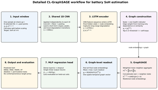
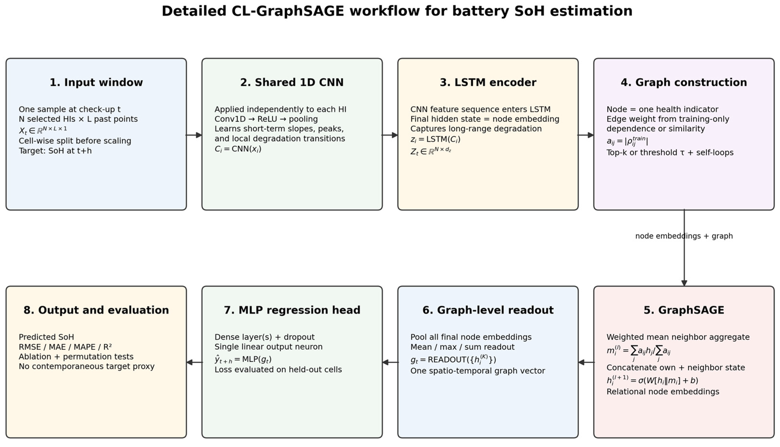
After the selection of the crucial HIs, the next step is to define the data processing methods and describe the model architecture. A Graph-Based Framework for SoH is developed using a Combined-Layer GraphSAGE (CL-GraphSAGE) (Figure 9). The framework leverages GNNs combined with CNNs and LSTM networks by utilizing both temporal and spatial features of HIs. This model architecture is designed to integrate multiple neural network techniques to capture comprehensive data characteristics.

Figure 9. Detailed workflow of the proposed CL-GraphSAGE model. The temporal sequence of each selected health indicator is first processed by a one-dimensional CNN to extract local degradation patterns. The CNN feature maps are transferred to an LSTM to obtain a temporal embedding for each health indicator. These embeddings form the initial node features of the fully connected health indicator graph. GraphSAGE performs mean neighborhood aggregation to capture relationships among the indicators. A graph-level readout combines the final node representations, and an MLP produces the predicted SoH [17].

4.1. Health Indicators Extraction and Filtration

The extraction of the relevant HIs from the raw battery data is done by creating an automated Python script. These indicators are derived from various stages of the charging and discharging processes and include features related to current, voltage, and time, as explained in Section 2.2. Once the HIs are extracted, they are filtered based on the discussion in Table 5 from Section 4.1. The eleven most sensitive HIs, which exhibit high sensitivity, are selected for further analysis.

Table 5. Selection and redundancy analysis of the original health indicators.

HI	Health Indicator	Mean $\mathit{r}$	Mean $\left|\mathit{r}\right|$
HI1	Cycling temperature	Retained	Temperature strongly affected capacity fade in the controlled cell comparisons.
HI2	Discharge capacity	Retained	Direct and consistent relationship with capacity-based SoH.
HI3	Charge capacity	Excluded	Highly redundant with discharge capacity; retaining both would duplicate capacity information.
HI4	Internal resistance	Retained	Provides complementary information concerning resistance growth and power capability.
HI5	Depth of discharge	Retained	Higher DoD produced greater capacity fade in the controlled comparison.
HI6	Middle SoC	Retained	The matched-cell comparison showed that middle SoC influences aging severity.
HI7	Discharge C-rate	Excluded	Insufficient variation in the experimental matrix for a robust independent assessment.
HI8	Charge C-rate	Excluded	Insufficient variation in the experimental matrix for a robust independent assessment.
HI9	Cycle number	Retained	Represents accumulated cycling and the progression of aging with time.
HI10	CC-charge current integral	Retained	Very high and consistent correlation with SoH; describes the evolution of the CC charging stage.
HI11	CV-charge current integral	Excluded	Correlation direction and magnitude varied between cells, and their information overlaps with other charge-stage indicators.
HI12	CC-CV charge-current integral	Excluded	Mathematically redundant because HI12 is the sum of HI10 and HI11.
HI13	Discharge-current integral	Retained	Strong positive relationship with SoH and direct description of the discharge process.
HI14	CC-charge voltage integral	Retained	Represents changes in the charging-voltage response during aging.
HI15	CV-charge voltage integral	Excluded	Describes the same CV stage as HI20 and was excluded to reduce redundancy between CV-related indicators.
HI16	Discharge-voltage integral	Retained	Captures changes in the discharge-voltage response and provides information complementary to current-derived indicators.
HI17	Discharge time	Excluded	Overlaps with discharge capacity and discharge-current information and showed a lower average relevance.
HI18	Charging time	Excluded	Lower and less consistent relationship with SoH and overlap with the charge-stage integrals.
HI19	CC-stage period	Retained	Physically interpretable charging-stage indicator with a moderate and relatively consistent relationship with SoH.
HI20	CV-stage period	Excluded	Strongly overlaps with the CV-voltage integral and other CV-stage information.

For the first step, eleven HIs are used, represented as a list of temporal data showing the evolution of values over multiple cycles. This temporal data serves as the input for the subsequent step. The data are divided into a training set and an evaluation set for model training. Specifically, sixteen cells are used for training and evaluation, with 80% of their data used for training and the remaining 20% for evaluation. After training, the model is tested using the complete data from the WLTC cell (cell 18) to assess its performance.

4.2. Graph Construction

The next phase involves constructing a graph structure from the filtered HIs. In this graph, each HI represents a node, and the edges between nodes are determined based on the similarity values between the HIs.

• Node definition:
  • Each selected HI is treated as a node.
  • The temporal sequence data of each HI serves as the node’s feature vector.
• Edge definition: the graph will be fully connected.

The graph G = (V, E) is thus formed, where V represents the set of nodes and E represents the set of edges. The graph captures both the temporal characteristics of individual HIs and the spatial interdependencies among them.

4.3. Temporal Feature Extraction Using CNN-LSTM

In the CL-GraphSAGE framework, the hybrid CNN-LSTM model plays a crucial role in extracting temporal features from the HIs of LiBs. This section includes a detailed description of the CNN and LSTM mechanisms, their functions, and how they work together to capture both local and long-term temporal dependencies within the data.

4.3.1. Convolutional Neural Networks (CNNs)

CNNs are a type of deep neural network that are particularly effective in processing data with a grid-like topology, such as time series data [28]. In the context of SoH prediction, the CNN is useful to extract local features from the temporal sequences of HIs. A CNN is composed of several layers, primarily convolutional layers, pooling layers, and fully connected layers. However, in this application, the focus is on convolutional layers and, to a lesser extent, pooling layers.

• Convolutional Layers:

Kernel and Convolution Operation: The core of a convolutional layer is the convolution operation, where a small matrix of weights, known as a kernel or filter, is slid over the input data. For time series data, this kernel typically moves along the time axis, performing element-wise multiplications of input data and adding the results to produce a feature map:

$$y_i={\sum }_{j=0}^{K-1}{w}_j{x}_{i+j}+b$$

(15)

where: K is the kernel size, w_j are kernel weights, and b is the bias.

• Feature Detection: The convolution operation allows the network to detect local patterns within the data, such as trends, peaks, or anomalies in the HIs. Multiple filters are used in each convolutional layer to capture different types of patterns within the same data sequence.
• Activation Function: An activation function such as ReLU (Rectified Linear Unit) is employed to introduce non-linearity, which enables the network to learn complex representations of the data:

$$f_i=ReLU\left(y_i\right)=\max \left(0,y_i\right)$$

(16)

Pooling Layers:

• Purpose: Pooling layers are typically used to reduce the dimensionality of the feature maps, which decreases the computational load and mitigates the risk of overfitting.
• Max Pooling: The most common type of pooling operation is max pooling, which down-samples the input by taking the maximum value within a pooling window (e.g., a sequence of time steps). This operation retains the most prominent features detected by the convolutional layers:

$$p_i=\max \left(f_i,f_{i+1},\dots ,f_{i+m-1}\right)$$

(17)

The CNN layers are designed to capture short-term dependencies and local patterns within the HIs. For example, changes in voltage or current over short time intervals can indicate critical information about the battery’s health.

4.3.2. Long Short-Term Memory Networks (LSTMs)

LSTM networks are a type of Recurrent Neural Network (RNN) designed to capture long-term dependencies in sequence data [29]. Unlike traditional RNNs, LSTMs are equipped with mechanisms to overcome the vanishing gradient problem, making them highly effective in learning from long sequences. An LSTM network consists of a series of LSTM units, each containing a set of gates that control the flow of information through the network:

• Cell State: The cell state acts as the memory of the network, carrying information across different time steps. It can be thought of as a conveyor belt that runs through the entire LSTM, with only minor linear interactions, which helps preserve the information across long sequences.

• Gates:

• Forget gate: This gate determines what portion of the previous cell state should be discarded. By taking the current input and the previous hidden state as inputs, it passes them through a sigmoid function to produce a value between 0 and 1. A value closer to 0 implies that the information is forgotten, while a value closer to 1 implies that the information is retained:

$$f_t=\sigma \left(W_f\left[h_{t-1},x_t\right]+b_f\right)$$

(18)

• Input Gate: The input gate controls the new information requirement to be added to the cell state. It functions similarly to the forget gate but focuses on the current input and how it should update the cell state:

$$i_t=\sigma \left(W_i\left[h_{t-1},x_t\right]+b_i\right)$$

(19)

• Output Gate: The output gate decides what the next hidden state should be. This state is used for predictions or as an input to the next time step. The output is determined by a combination of the current input, the cell state, and the previous hidden state, again passed through a sigmoid function:

$$o_t=\sigma \left(W_o\left[h_{t-1},x_t\right]+b_o\right)$$

(20)

State Updates:

• Cell State Update: The forget and input gates work together to update the cell state, ensuring that the network retains useful information and discards irrelevant information.
  • Hidden State Update: The updated cell state, along with the output gate, produces the hidden state that carries the learned information to the next LSTM unit or to the output layer if it is the final time step.

LSTM networks are critical for capturing long-term dependencies in the HIs data. The LSTM’s ability to retain important historical information while filtering out less relevant data makes it ideal for tasks where understanding long-term trends is essential.

By combining CNNs and LSTMs, the model can effectively learn from both short-term fluctuations and long-term trends in the battery’s operational data. This dual approach ensures that the temporal features extracted are both rich and representative of the complex processes underlying battery degradation [30,31].

The temporal features obtained from the CNN-LSTM model are utilized as the node features in the graph structure of the CL-GraphSAGE framework. Each node in the graph represents an HI, and its feature vector is the output of the CNN-LSTM model.

4.3.3. Connection and Feature Transmission in the CL-GraphSAGE Architecture

The CNN, LSTM, and GraphSAGE modules are connected sequentially rather than operating as independent or parallel prediction branches. For each model sample, the historical values of every selected health indicator are organized as an individual temporal sequence. Let the sequence of health indicator i over L successive check-ups be denoted by

$${\mathbf{x}}_i\in {\mathbb{R}}^{L\times 1}$$

(21)

First, a one-dimensional CNN is applied along the temporal axis:

$${\mathbf{C}}_i=\mathrm{C}\mathrm{N}\mathrm{N} \left({\mathbf{x}}_i\right)$$

(22)

The convolutional filters identify short-range patterns such as local slopes, fluctuations, abrupt changes, and short-term degradation trends. The resulting ordered feature maps are retained as a sequence and transferred to the LSTM:

$${\mathbf{z}}_i=\mathrm{L}\mathrm{S}\mathrm{T}\mathrm{M} \left({\mathbf{C}}_i\right)$$

(23)

where, ${\mathbf{z}}_i$ is the final temporal representation of a health indicator $i$. Thus, the CNN extracts local temporal characteristics, while the LSTM combines these characteristics over a longer historical interval.

The temporal representations of all $N$ selected health indicators are subsequently stacked to form the initial graph node-feature matrix:

$${\mathbf{H}}^{\left(0\right)}={\left[{\mathbf{z}}_1,{\mathbf{z}}_2,\dots ,{\mathbf{z}}_N\right]}^{\mathrm{T}}$$

(24)

Each row of ${\mathbf{H}}^{\left(0\right)}$ therefore corresponds to one health indicator node. The CNN-LSTM output is not directly used to calculate SoH; instead, it is transferred to GraphSAGE as the initial node representation.

In the present implementation, the health indicator graph is fully connected. Therefore, each node can exchange information with all the other health indicator nodes. At GraphSAGE layer $l$, the neighborhood representation of the node $i$ is obtained using mean aggregation:

$${\mathbf{m}}_i^{\left(l\right)}={\displaystyle \frac{1}{\left|\mathcal{N}\left(i\right)\right|}}{\sum }_{j\in \mathcal{N}\left(i\right)}{\mathbf{h}}_j^{\left(l\right)}$$

(25)

The aggregated neighborhood information is combined with the node’s own representation:

$${\mathbf{h}}_i^{\left(l+1\right)}=\sigma \left({\mathbf{W}}^{\left(l\right)}\left[{\mathbf{h}}_i^{\left(l\right)}\parallel {\mathbf{m}}_i^{\left(l\right)}\right]+{\mathbf{b}}^{\left(l\right)}\right)$$

(26)

where, $\parallel$ denotes concatenation and $\sigma$ is the activation function. This operation allows the representation of each health indicator to include complementary information from the remaining current, voltage, time, resistance, and operating condition indicators.

After the final GraphSAGE layer, the node representations are combined using a graph-level readout operation:

$$\mathbf{g}=\mathrm{R}\mathrm{E}\mathrm{A}\mathrm{D}\mathrm{O}\mathrm{U}\mathrm{T} \left({\mathbf{h}}_1^{\left(K\right)},{\mathbf{h}}_2^{\left(K\right)},\dots ,{\mathbf{h}}_N^{\left(K\right)}\right)$$

(27)

where, $K$ is the number of GraphSAGE layers. The resulting graph vector $\mathbf{g}$, which contains both temporal information from the CNN-LSTM block and relational information from GraphSAGE, is passed to the MLP regression head:

$$\widehat{\mathrm{S}\mathrm{o}\mathrm{H}}=\mathrm{M}\mathrm{L}\mathrm{P} \left(\mathbf{g}\right)$$

(28)

Consequently, the complete feature-transmission pathway can be summarized as

$${\left\{{\mathbf{x}}_i\right\}}_{i=1}^N\stackrel{\mathrm{C}\mathrm{N}\mathrm{N}}{\to }{\left\{{\mathbf{C}}_i\right\}}_{i=1}^N\stackrel{\mathrm{L}\mathrm{S}\mathrm{T}\mathrm{M}}{\to }{\mathbf{H}}^{\left(0\right)}\stackrel{\mathrm{G}\mathrm{r}\mathrm{a}\mathrm{p}\mathrm{h}\mathrm{S}\mathrm{A}\mathrm{G}\mathrm{E}}{\to }{\mathbf{H}}^{\left(K\right)}\stackrel{\mathrm{R}\mathrm{E}\mathrm{A}\mathrm{D}\mathrm{O}\mathrm{U}\mathrm{T}}{\to }\mathbf{g}\stackrel{\mathrm{M}\mathrm{L}\mathrm{P}}{\to }\widehat{\mathrm{S}\mathrm{o}\mathrm{H}}$$

(29)

4.4. Spatial Feature Extraction Using GraphSAGE

GraphSAGE is employed to aggregate and propagate information across the nodes in the graph. This process enhances the node features by incorporating information from neighboring nodes, thereby capturing the spatial interdependencies among HIs.

• Aggregation Function
  • For each node, an aggregation function computes a summary of the features from its neighboring nodes.
  • Mean aggregation is typically used, where the features of the neighboring nodes are averaged.
• Update Function
  • The aggregated features are combined with the node’s own features to update its state. Mean aggregation is typically used, where the features of the neighboring nodes are averaged.
  • This update is performed through a neural network layer, which learns the optimal combination of features.

The updated node features, after several iterations of aggregation and update, provide a comprehensive representation that includes both temporal and spatial information.

4.5. SoH Prediction Using Multilayer Perceptron (MLP)

The final step in the CL-GraphSAGE framework is the prediction of the SoH using an MLP. This process involves transforming the global representation of the graph, which encapsulates both temporal and spatial features, into a final SoH prediction.

4.5.1. Global Graph Representation

The global representation is a crucial intermediary that aggregates the information embedded in all the nodes of the graph. This is achieved through a readout function that consolidates the features of each node into a single, comprehensive feature vector representing the entire graph.

• Readout Function: The readout function aggregates the node features, often using methods like max pooling, mean pooling, or sum pooling. Max pooling is often used to retain the most salient features across all nodes, ensuring that the critical information is preserved.
• Formation of Global Graph Representation: After pooling, the resulting vector serves as a compact representation of the graph, encapsulating the critical temporal and spatial information necessary for accurate SoH prediction.

4.5.2. SoH Prediction with MLP

The global graph representation is fed into a Multilayer Perceptron (MLP), which consists of multiple dense layers that process the vector to generate the final prediction.

• Output layer: Produces the predicted SoH value.
• The forward propagation process of the proposed CL-GraphSAGE framework can be summarized as:

  $$SoH=MLP\left(GraphSAGE\left(LSTM\left(CNN\left(X\right)\right),G\right)\right)$$

  (30)
• Training: The MLP is trained to minimize a loss function, with the Mean Squared Error (MSE) used in this case. MSE measures the average squared difference between predicted ($\widehat{y_i})$ and actual values ($y_i)$, placing greater emphasis on larger errors. It is defined as:

  $$\mathrm{MSE}={\displaystyle \frac{1}{n}}{\sum }_{i=1}^n{\left(y_i-\widehat{y_i}\right)}^2$$

  (31)

4.5.3. Training and Evaluation of the Model

The metrics for the training and evaluation of the model are described in Table 6.

Table 6. Evaluation metrics for the model.

Code	Python 3.8. PyTorch V2.10.0 and PyTorch 2.10 Geometric
Hardware	Apple M1 Pro chip with 8-core CPU, 14-core GPU
Optimizer	Adam
Huber Loss objective function	1
Training epochs	1500
Batch size	32
Learning Rate	0.0008

To evaluate the performance of the machine learning model, three key metrics were utilized: MSE, along with the Mean Absolute Percentage Error (MAPE), and the coefficient of determination (R²). Together, these metrics offer a comprehensive understanding of the model’s predictive performance.

5. Validation and Discussions

The developed GNN-based degradation model was trained and evaluated using data from 16 individual NMC cells. The model’s performance in the WLTC test will be analyzed, highlighting its effectiveness in predicting battery degradation under complex, real-world conditions. The results will be discussed in terms of accuracy, consistency, and any observed discrepancies, providing a critical evaluation of the model’s overall reliability and potential for practical application.

5.1. Analysis of the Model Performance

5.1.1. Training and Evaluation Performance

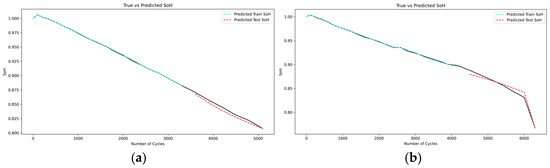
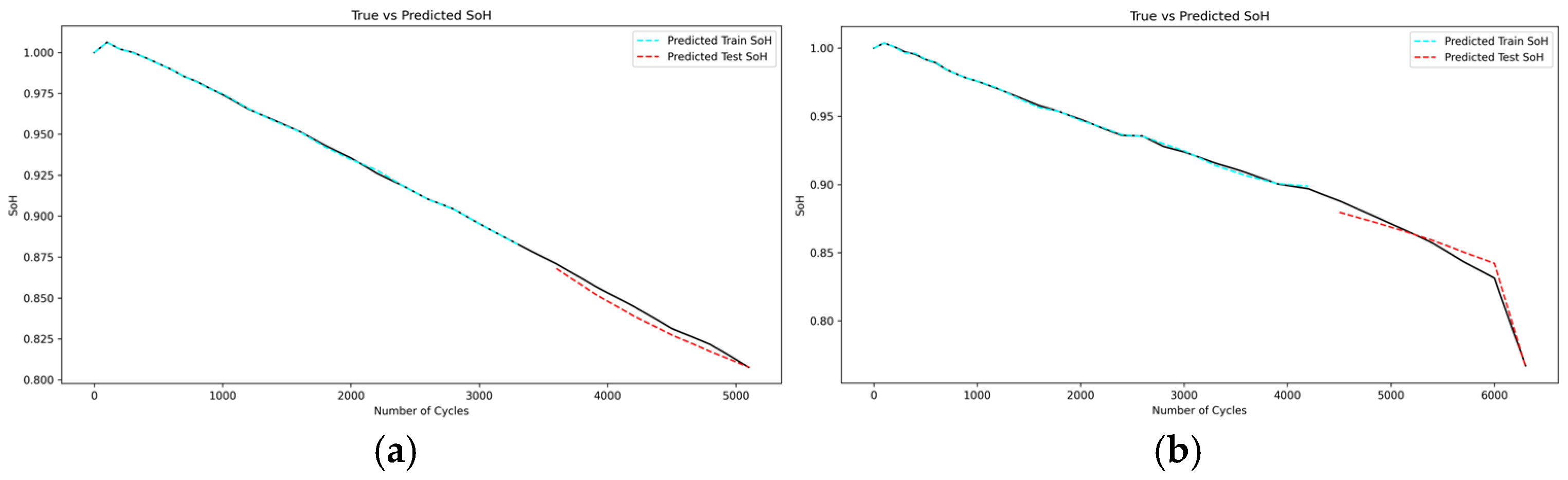
During the training and evaluation phases, it is observed that the model performs exceptionally well with many cells (Figure 10). For these cells, the model effectively learns the degradation patterns from the first 80% of the data and successfully extrapolates this knowledge to the unseen data. However, there are other cases where the model achieves good predictions during training but fails to generalize effectively. This issue may be attributed to overfitting during the training process.

Figure 10. Training and validation results of (a) Cell 5; (b) Cell 6.

5.1.2. Test Performance

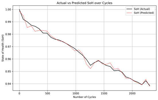
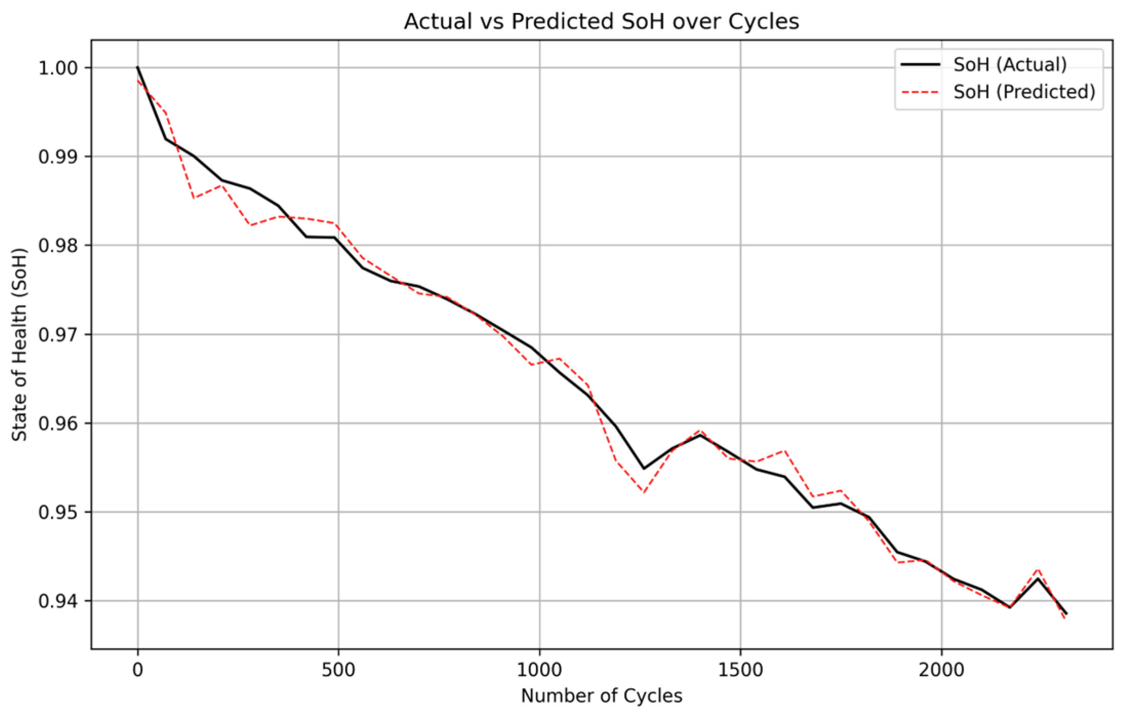
This is the crucial stage where the model’s practical utility is assessed. Here, data that the model has not previously encountered are used, with a cycling profile that is unseen. While the model was trained using the same HI, the temporal cycling pattern is distinct. To evaluate the model, the entire data series of cell 18 with the WLTC profile is used, the His are extracted, and the eleven most correlated with the SoH are selected as inputs to the model. Figure 11 compares the model’s predicted SoH with the actual SoH, while Table 7 lists the corresponding performance metrics for the degradation model.

Figure 11. WLTC profile SoH prediction result (for cell 18).

Table 7. Performance Metrics for the GNN-Based Degradation Model.

Metric	Value
Mean Squared Error (MSE)	3.23 × 10−6
Mean Absolute Error (MAE)	0.0014
Coefficient of Determination (R2)	0.989

The proposed predictive model performance could be expressed as a percentage of SoH corresponding to RMSE 0.18%, MAE 0.14%, and R² 0.989. Ma et al. [32] reported strong results with a hybrid CNN-LSTM on the CALCE and NASA 18650 datasets. For their best test case, the model yields RMSE 0.24%, MAE 0.18%, and R² = 0.998. On other test batteries, their RMSE/MAE range up to 0.48%/0.44%. Other similar models have produced similar results, like 0.3% reported by Kim et al. [33] with the CALCE dataset, 0.4% was reported by Wang et al. [34] using the MIT dataset, but with only LSTM-GNN layers, and 0.63% reported by Zhou et al. [20] using the MIT dataset with a convolutional graph network. Thus, in terms of RMSE, the proposed model attains better results compared with the literature.

6. Conclusions and Future Work

The accurate prediction of the SoH of lithium-ion batteries is becoming increasingly vital due to their widespread use in electric vehicles and energy storage systems. In this research work, a deep learning model based on graph neural networks was developed to predict the SoH of commercial NMC pouch cells. The model was trained and validated using a high-quality dataset obtained from extensive experimental work for more than 2 years. These tests covered batteries operated under various conditions, and a variety of health indicators were extracted to obtain meaningful insights about their relationship with the degradation of the battery.

The developed model includes different deep learning models to be able to extract not only temporal but also local features from the dataset. This involves CNN, LSTM, and GraphSAGE. Key performance metrics, including an R² of 0.989 and an MAE of 0.14%, highlight the advantages of the GNN approach in accurately modeling the complex interactions influencing battery degradation. Such models could be deployed for a cloud-connected real-time edge battery management system for advanced prognosis.

The applicability or generalization of the model could be tested for another type of NMC dataset or even for other types of chemistries like LFP, NCA, etc. The model performance could further be improved by optimizing the nodes and networks.

References

- Ralls, A.M.; Leong, K.; Clayton, J.; Fuelling, P.; Mercer, C.; Navarro, V.; Menezes, P.L. The Role of Lithium-Ion Batteries in the Growing Trend of Electric Vehicles. Materials 2023, 16, 6063. [Google Scholar] [CrossRef] [PubMed]
- Nkembi, A.A.; Simonazzi, M.; Santoro, D.; Cova, P.; Delmonte, N. Comprehensive Review of Energy Storage Systems Characteristics and Models for Automotive Applications. Batteries 2024, 10, 88. [Google Scholar] [CrossRef]
- Zubi, G.; Dufo-López, R.; Carvalho, M.; Pasaoglu, G. The lithium-ion battery: State of the art and future perspectives. Renew. Sustain. Energy Rev. 2018, 89, 292–308. [Google Scholar] [CrossRef]
- Collin, R.; Miao, Y.; Yokochi, A.; Enjeti, P.; Von Jouanne, A. Advanced electric vehicle fast-charging technologies. Energies 2019, 12, 1839. [Google Scholar] [CrossRef]
- Miao, Y.; Hynan, P.; Von Jouanne, A.; Yokochi, A. Current Li-ion battery technologies in electric vehicles and opportunities for advancements. Energies 2019, 12, 1074. [Google Scholar] [CrossRef]
- Tanim, T.R.; Yang, Z.; Finegan, D.P.; Chinnam, P.R.; Lin, Y.; Weddle, P.J.; Bloom, I.; Colclasure, A.M.; Dufek, E.J.; Wen, J.; et al. A Comprehensive Understanding of the Aging Effects of Extreme Fast Charging on High Ni NMC Cathode. Adv. Energy Mater. 2022, 12, 2103712. [Google Scholar] [CrossRef]
- Hosen, S.; Kalogiannis, T.; Youssef, R.; Karimi, D.; Behi, H.; Jin, L.; Van Mierlo, J.; Berecibar, M. Twin-model framework development for a comprehensive battery lifetime prediction validated with a realistic driving profile. Energy Sci. Eng. 2021, 9, 2191–2201. [Google Scholar] [CrossRef]
- Hosen, M.S.; Pirooz, A.; Kalogiannis, T.; He, J.; Van Mierlo, J.; Berecibar, M. A Strategic Pathway from Cell to Pack-Level Battery Lifetime Model Development. Appl. Sci. 2022, 12, 4781. [Google Scholar] [CrossRef]
- Olmos, J.; Gandiaga, I.; Saez-de-Ibarra, A.; Larrea, X.; Nieva, T.; Aizpuru, I. Modelling the cycling degradation of Li-ion batteries: Chemistry influenced stress factors. J. Energy Storage 2021, 40, 102765. [Google Scholar] [CrossRef]
- Gasper, P.; Saxon, A.; Shi, Y.; Endler, E.; Smith, K.; Thakkar, F.M. Degradation and modeling of large-format commercial lithium-ion cells as a function of chemistry, design, and aging conditions. J. Energy Storage 2023, 73, 109042, Correction in J. Energy Storage 2024, 84, 110884. https://doi.org/10.1016/j.est.2024.110884. [Google Scholar] [CrossRef]
- Dong, G.; Wei, J. A physics-based aging model for lithium-ion battery with coupled chemical/mechanical degradation mechanisms. Electrochim. Acta 2021, 395, 139133. [Google Scholar] [CrossRef]
- Yavuz, H.; Akyildiz, A.; Gulbahce, M.O. A Comprehensive Review of Physics-Based Battery Models and Comparing Different Physics-Based Models for Various Chemistries. Turk. J. Electr. Power Energy Syst. 2024, 4, 108–117. [Google Scholar] [CrossRef]
- Hosen, M.S.; Youssef, R.; Kalogiannis, T.; Van Mierlo, J. Battery cycle life study through relaxation and forecasting the lifetime via machine learning. J. Energy Storage 2021, 40, 102726. [Google Scholar] [CrossRef]
- Xu, H.; Wu, L.; Xiong, S.; Li, W.; Garg, A.; Gao, L. An improved CNN-LSTM model-based state-of-health estimation approach for lithium-ion batteries. Energy 2023, 276, 127585. [Google Scholar] [CrossRef]
- Zhao, F.M.; Gao, D.X.; Cheng, Y.M.; Yang, Q. Application of state of health estimation and remaining useful life prediction for lithium-ion batteries based on AT-CNN-BiLSTM. Sci. Rep. 2024, 14, 29026. [Google Scholar] [CrossRef] [PubMed]
- Liu, G.; Deng, Z.; Xu, Y.; Lai, L.; Gong, G.; Tong, L.; Zhang, H.; Li, Y.; Gong, M.; Yan, M.; et al. Lithium-Ion Battery State of Health Estimation Based on CNN-LSTM-Attention-FVIM Algorithm and Fusion of Multiple Health Features. Appl. Sci. 2025, 15, 7555. [Google Scholar] [CrossRef]
- Yao, X.Y.; Chen, G.; Pecht, M.; Chen, B. A novel graph-based framework for state of health prediction of lithium-ion battery. J. Energy Storage 2023, 58, 106437. [Google Scholar] [CrossRef]
- Louis, S.Y.; Siriwardane, E.M.D.; Joshi, R.P.; Omee, S.S.; Kumar, N.; Hu, J. Accurate Prediction of Voltage of Battery Electrode Materials Using Attention-Based Graph Neural Networks. ACS Appl. Mater. Interfaces 2022, 14, 26587–26594. [Google Scholar] [CrossRef] [PubMed]
- Wu, W.; Chen, Z.; Liu, W.; Pan, E. Correlation based-graph neural network for health prognosis of non-fully charged and discharged lithium-ion batteries. J. Power Sources 2025, 629, 235984. [Google Scholar] [CrossRef]
- Zhou, K.Q.; Qin, Y.; Yuen, C. Graph neural network-based lithium-ion battery state of health estimation using partial discharging curve. J. Energy Storage 2024, 100, 113502. [Google Scholar] [CrossRef]
- Zhao, Y.; Behdad, S. State-of-Health Estimation for Sustainable Electric Vehicle Batteries Using Temporal- Enhanced Self-Attention Graph Neural Networks. J. Energy Resour. Technol. Trans. ASME 2024, 146, 062102. [Google Scholar] [CrossRef]
- Benesty, J.; Chen, J.; Huang, Y.; Cohen, I. Pearson correlation coefficient. In Noise Reduction in Speech Processing; Springer: Berlin/Heidelberg, Germany, 2009; Volume 2, pp. 1–4. [Google Scholar]
- Jalkanen, K.; Karppinen, J.; Skogström, L.; Laurila, T.; Nisula, M.; Vuorilehto, K. Cycle aging of commercial NMC/graphite pouch cells at different temperatures. Appl. Energy 2015, 154, 160–172. [Google Scholar] [CrossRef]
- Ma, S.; Jiang, M.; Tao, P.; Song, C.; Wu, J.; Wang, J.; Deng, T.; Shang, W. Temperature effect and thermal impact in lithium-ion batteries: A review. Prog. Nat. Sci. Mater. Int. 2018, 28, 653–666. [Google Scholar] [CrossRef]
- Severson, K.A.; Attia, P.M.; Jin, N.; Perkins, N.; Jiang, B.; Yang, Z.; Chen, M.H.; Aykol, M.; Herring, P.K.; Fraggedakis, D.; et al. Data-driven prediction of battery cycle life before capacity degradation. Nat. Energy 2019, 4, 383–391. [Google Scholar] [CrossRef]
- Ecker, M.; Gerschler, J.B.; Vogel, J.; Käbitz, S.; Hust, F.; Dechent, P.; Sauer, D.U. Development of a lifetime prediction model for lithium-ion batteries based on extended accelerated aging test data. J. Power Sources 2012, 215, 248–257. [Google Scholar] [CrossRef]
- Mussa, A.S.; Klett, M.; Behm, M.; Lindbergh, G.; Lindström, R.W. Fast-charging to a partial state of charge in lithium-ion batteries: A comparative ageing study. J. Energy Storage 2017, 13, 325–333. [Google Scholar] [CrossRef]
- Sun, S.; Sun, J.; Wang, Z.; Zhou, Z.; Cai, W. Prediction of Battery SOH by CNN-BiLSTM Network Fused with Attention Mechanism. Energies 2022, 15, 4428. [Google Scholar] [CrossRef]
- Hu, X.; Xu, L.; Lin, X.; Pecht, M. Battery Lifetime Prognostics. Joule 2020, 4, 310–346. [Google Scholar] [CrossRef]
- Huang, J.; He, T.; Zhu, W.; Liao, Y.; Zeng, J.; Xu, Q.; Niu, Y. A lithium-ion battery SOH estimation method based on temporal pattern attention mechanism and CNN-LSTM model. Comput. Electr. Eng. 2025, 122, 109930. [Google Scholar] [CrossRef]
- Li, W.; Li, Y.; Garg, A.; Gao, L. Enhancing real-time degradation prediction of lithium-ion battery: A digital twin framework with CNN-LSTM-attention model. Energy 2024, 286, 129681. [Google Scholar] [CrossRef]
- Ma, X.; Ding, X.; Tian, C.; Tian, C.; Zhu, R. Estimation of Lithium-Ion Battery State of Health-Based Multi-Feature Analysis and Convolutional Neural Network–Long Short-Term Memory. Sustainability 2025, 17, 4014. [Google Scholar] [CrossRef]
- Kim, W.H.J.; Chung, Y.M.; Stinner, B. State of health prediction of lithium-ion batteries with adaptive loss-based graph neural network. J. Energy Storage 2025, 124, 116637. [Google Scholar] [CrossRef]
- Wang, Z.; Yang, F.; Xu, Q.; Wang, Y.; Yan, H.; Xie, M. Capacity estimation of lithium-ion batteries based on data aggregation and feature fusion via graph neural network. Appl. Energy 2023, 336, 120808. [Google Scholar] [CrossRef]
Disclaimer/Publisher’s Note: The statements, opinions and data contained in all publications are solely those of the individual author(s) and contributor(s) and not of MDPI and/or the editor(s). MDPI and/or the editor(s) disclaim responsibility for any injury to people or property resulting from any ideas, methods, instructions or products referred to in the content. |
© 2026 by the authors. Licensee MDPI, Basel, Switzerland. This article is an open access article distributed under the terms and conditions of the Creative Commons Attribution (CC BY) license.