PSO-LSTM-Based Ultra-Short-Term Load Forecasting Study for Solar Heating System

Abstract

To address issues such as unstable heating loads, uneven heat consumption, and precise heating in solar heating systems, efficient and accurate heating load forecasting is essential. A suitable solar heating system model was established using the TRNSYS18 thermodynamic simulation platform. Taking a building in Alar City, Xinjiang, as the research subject, ultra-short-term prediction data parameters for the area were obtained. Using the acquired data parameters and historical heating load data as inputs, the particle swarm optimization (PSO) algorithm was employed to optimize the LSTM neural network, establishing a prediction model based on the PSO-LSTM neural network. For load forecasting in 7 min ultra-short-term time series, both the LSTM neural network model and the PSO-LSTM neural network prediction model underwent optimization. Through simulation experiments verifying indoor temperature, heat collection, and energy consumption, two model error evaluation metrics were used as results. Comparative analysis revealed that the PSO-LSTM model achieved a 3.3–86.7% increase in R² compared to the LSTM model, a 38.2–84.8% reduction in RMSE, a 57.8–91.1% decrease in MAE, and a 58–90.3% reduction in MAPE. The research results demonstrate the PSO-LSTM model’s effectiveness in southern Xinjiang, confirming its superiority as a forecasting model. This provides data support for operational adjustments and load forecasting in solar heating systems.

1. Introduction

In recent years, while the scale of construction in the Xinjiang region has continued to expand, higher requirements have been placed on energy conservation and environmental protection. These requirements have prompted the region to actively promote the development and popularization of areas such as heat supply and clean heating, and the coverage of heat supply in rural areas has been increasing year by year. With the improvement of people’s living standards, rural residents’ expectations for the quality of heating are also rising. However, at present, some rural areas are still using the heat source side of the control-oriented management model; this more relaxed mode of operation leads to the existence of uneven heat and other problems (Dong, 2022 [1]). In order to realize “on-demand” and “accurate heat supply” and improve the efficiency of heat supply and service quality, most studies have adopted persistence (Sarmas et al., 2022 [2]; Visser et al., 2022 [3]; Long et al., 2014 [4]), physics (Mayer and Gróf, 2021 [5]; Huang et al., 2021 [6]), hybrid integration (Fraccanabbia et al., 2020 [7]; Kamble et al., 2020 [8]), statistics, machine learning (Subramanian et al., 2023 [9]; Anand et al., 2023 [10]; Kapilan et al., 2022 [11]), and deep learning (Ahmed et al., 2020 [12]). With the continuous development of computer science and technology, many modeling methods based on hybrid neural networks are widely used. (Yan et al., 2023 [13]) achieved better results by establishing an ALSTM network to forecast the outlet temperature of the trough collector. Song Building (Song et al., 2021 [14]) proposed a convolutional neural network-based long-time memory neural network (CNN-LSTM) hybrid network heat load forecasting model with feature extraction along both spatio-temporal and temporal dimensions. Experiments show that the CNN-LSTM-based hybrid model has significant superiority in terms of computational accuracy. (Kim and Cho, 2019 [15]) and (Raf et al., 2021 [16]) also built a series of CNN-LSTM models, proving that the method has higher prediction accuracy compared to a single neural network. However, the method has the problems of a single structure, slow convergence of the algorithm, fixed input characteristics, etc., which make it difficult to realize the rapid adjustment of the input characteristic parameters and meet the needs of engineering applications. To enhance the accuracy and reliability of short-term load forecasting for solar heating systems in southern Xinjiang, this study proposes integrating the particle swarm optimization (PSO) algorithm into long short-term memory (LSTM) neural networks to achieve automatic optimization of hyperparameters (Chen et al., 2025 [17]). This approach is primarily driven by the following two factors: First, the inherent characteristics of the particle swarm algorithm make it well-suited for practical applications. With a clear conceptual framework, minimal parameters, and ease of implementation, it possesses strong global optimization capabilities. This effectively prevents local optima during the optimization process, providing the LSTM with an efficient set of hyperparameter combinations (Badjan et al., 2024 [18]). Compared to other algorithms, the PGA generally exhibits good convergence, effectively reducing model adjustment time and costs. Second, integrating PGA with LSTM technology can effectively address key challenges in solar heating systems in southern Xinjiang. Due to influences such as intense local solar radiation, large temperature differentials, and transient cloud variations, the thermal load exhibits strong nonlinearity and volatility. Traditional manual parameter tuning struggles to adapt to these complex dynamic characteristics. By introducing the particle swarm algorithm into autonomous optimization, this approach ensures precise configuration of LSTM model parameters—including structure and learning rates—enabling enhanced dynamic feature capture and time-varying correlation modeling. This achieves higher-precision, more robust seven-minute ultra-short-term heating load forecasting, providing reliable data support for system heating and energy-saving optimization. As part of the research and application of solar dual-mode heating key technology for the “beautiful company” national research and development project, the main task of this paper is to realize the ultra-short-term accurate prediction of district heating load, and the research results of this paper will provide the theoretical basis and technical support for the optimization of the centralized heating system in Xinjiang.

2. TRNSYS Simulation Model

TRNSYS (Transient System Simulation Program) is a transient system simulation program developed by SEL at the University of Wisconsin, and the latest version is Ver. 18. In this paper, according to the connection relationship between the devices in the solar heating system, the simulation model of the solar heating system is completed in this thermodynamic simulation platform construction.

2.1. Mathematical Model

2.1.1. Mathematical Model of Collector

In this paper, the collector device in the solar dual-mode heating system is a vacuum tube solar collector, and this paper uses the thermodynamic simulation platform to carry out numerical simulation of the solar heating system, and verifies the validity of the model of the solar heating system through the establishment of the mathematical model of operation and regulation and the comparative analysis with the data of the experimental platform. The model can be calculated to obtain the collector inlet and outlet temperatures, the effective heat gain value of the collector. Under steady-state conditions, the effective heat gain of the solar collector is equal to the energy it absorbs from solar radiation minus the heat lost to the outside world. The energy balance equation for vacuum tube solar collector at any moment is the following:

$${\displaystyle \frac{d{t}_{pc}}{ds}}+{\displaystyle \frac{\left(2m_l{c}_{pc}+A_l{U}_L\right)}{M_{C_{pc}}}}={\displaystyle \frac{2m_l{t}_{inc}}{M}}+{\displaystyle \frac{I{\left(\tau \alpha \right)}_{\theta }{A}_2}{M_{C_{pc}}}}+{\displaystyle \frac{A_l{U}_L{t}_{am}}{M_{C_{pc}}}}+{\displaystyle \frac{m_l}{M}}\left(\omega J\epsilon -{\displaystyle \frac{\omega J{m}_c}{m_l}}\right)$$

(1)

Among them are the following:

$$J={\displaystyle \frac{2I{r}_1{\left(\tau \alpha \right)}_{\theta }}{M_{C_{pc}}}}$$

(2)

$$m_c=0.5\pi r_1^2\rho \sqrt{\dot{r}gI{\left(\tau \alpha \right)}_{\theta }{r}_f\omega \mathit{sin}\beta /\left(2{\mu }_{C_{pc}}\right)}$$

(3)

Style: $t_{am}$—outdoor temperature (°C); $s$—time (s); $t_{pc}$—average temperature of the collector plate (°C); $C_{pc}$—specific heat capacity of the fluid medium (kJ/(kg·°C)); $m_l$—is the mass flow rate (kg/s); $U_L$—heat loss coefficient; $I$—radiation intensity (W/m²); $M$—heat collection system water storage (kg); ${\left(\tau \alpha \right)}_{\theta }$—the product of absorption rate and transmission rate; $A_l$, $A_2$—heat dissipation, radiation area (m²); $m_c$—flow rate under natural convection (kg/s); $\beta$—inclination angle, degree; $\mathsf{\epsilon }$—proportion of thermal fluid in the collector tube; $r_1$—diameter of the tube (m); $\rho$—density of the work mass (kg/m); $\mu$—dynamic viscosity (Pa·s).

2.1.2. Mathematical Modeling of Thermal Storage Tanks

In this paper, a layered thermal storage tank is used for the solar heating system. In modeling the hierarchical thermal storage tank, the tank is divided into several tiers along the vertical direction and the water temperature within each tier is assumed to be uniform. The principle of conservation of energy is followed between the tiers. Equipment parameters to be input for modeling include the tank volume and the surface heat loss coefficient. The model allows the calculation of values such as the average temperature of the tank, and the thermal efficiency at each inlet and outlet.

The energy balance equation for the thermal storage tank is the following:

$${\displaystyle \frac{d{T}_{\mathit{tank}}}{d\tau }}={\displaystyle \frac{Q_{\mathit{in},\mathit{tank}}-Q_{\mathit{out},\mathit{tank}}}{C_{\mathit{tank}}}}$$

(4)

The heat loss equation for the thermal storage tank is the following:

$$Q_{\mathit{loss},\mathit{edges},j}=A_{\mathit{edges},j}{U}_{\mathit{edges}}\left(T_{\mathit{tank},j}-T_{\mathit{env},\mathit{edges}}\right)$$

(5)

The corresponding energy balance equation for each layer of the tank is the following:

$$Q_{\mathit{cond},j}=k_j{A}_j{\displaystyle \frac{T_j-T_{j-1}}{L_{\mathit{cond},j}}}+k_{j-1}{A}_{j-1}{\displaystyle \frac{T_j-T_{j-1}}{L_{\mathit{cond},j-1}}}$$

(6)

Style: $A_j$—surface area of heat loss at node j of the heat storage tank (m²); U—heat loss coefficient of the heat storage tank; $T_{\mathit{tank},j}$—temperature of layer j of the heat storage tank (°C); $T_{\mathit{env}}$—ambient temperature around the heat storage tank (°C).

2.1.3. Mathematical Model of Auxiliary Heat Source

Air source heat pump is used as an auxiliary heat source. When the system cannot utilize solar energy for heating, the air source heat pump is turned on for heating, which can effectively ensure that the indoor temperature is in the comfortable temperature range. Heat pumps for heating can effectively ensure that the indoor temperature is in the comfortable temperature range. In this paper, the air source heat pump model is established in TRNSYS, and its performance parameters are imported through external files. The energy efficiency ratio of air source heat pump is calculated as in Formula (7):

$$\mathrm{COP}=\left(\mathsf{\Sigma }{Q}_{\mathit{ASHP}}·\mathsf{\Delta }\tau \right)/\left(\mathsf{\Sigma }{E}_{\mathit{ASHP}}·\mathsf{\Delta }\tau \right)$$

(7)

Style: $\mathrm{COP}$—energy efficiency ratio of air source heat pumps; $Q_{\mathit{ASHP}}$—air source heat pump heating capacity (kW); $E_{\mathit{ASHP}}$—electrical energy input (kW) for air source heat pumps; $\mathsf{\Delta }\tau$—air source heat pump operating hours.

2.1.4. Mathematical Model of Radiator

In the solar heating system described in this paper, cast iron type radiators are selected for the end heating devices. Hot water flowing through these radiators heats up their surfaces and subsequently transfers energy to the room by convection and radiation, thereby taking up the indoor heat load and enhancing the indoor temperature and comfort. To calculate this process, the model requires inputs of heat transfer coefficients as well as room temperature parameters. Based on these inputs, the model is able to output values such as the heat supply of the radiator and the temperature of the radiator surface. According to the law of conservation of energy, for radiators, the difference between the heat brought in by the water supply and the heat transfer from the radiator to the room is equal to the net heat of the hot water it stores. So the mathematical model is obtained as the following:

$$C_S{\displaystyle \frac{d{T}_h}{\mathit{dt}}}=c_w\dot{m}\left(T_g-T_h\right)-K_s{F}_s\left({\displaystyle \frac{T_g+T_h}{2}}-T_r\right)$$

(8)

Style: $C_S$—heat capacity of the radiator, J/°C; $c_w$—specific heat capacity of the fluid (J/kg·°C); $F_s$—heat transfer area (m²); $K_s$—heat transfer coefficient (W/(m²·°C)); $T_g,T_h$—radiator inlet and outlet water temperatures (°C). $T_r$—room indoor temperature (°C).

The heat transfer from the radiator is the following:

$$\mathrm{q}=c{\left(T_s-T_r\right)}^n$$

(9)

Style: $T_s$—Radiator surface temperature (°C); $c$—Unit capacity constant; $n$—Unit capacity index.

2.1.5. Mathematical Model of Circulating Water Pump

As the power device of the system, the water pump plays a key role in the solar heating system. The system contains two types of collectors circulating water pumps and end heating circulating water pumps. For the collector circulating water pumps, this paper adopts the start-stop control strategy, i.e., the power and flow rate of the pump are kept constant. For the end heating circulating water pump, variable flow control is implemented, and its flow rate will be adjusted accordingly to the received control signal, and the corresponding power will also be changed. The circulating water pump operating efficiency formula is as follows:

$${\eta }_{\mathit{pumping}}={\displaystyle \frac{{\eta }_{\mathit{overall}}}{{\eta }_{\mathit{motor}}}}$$

(10)

Style: ${\eta }_{pumping}$—pump operating efficiency; ${\eta }_{overall}$—total pump efficiency; ${\eta }_{motor}$—pump motor efficiency.

2.1.6. Mathematical Modeling of Room Heat Balance

Room heat balance refers to the change of air temperature in the room due to different forms of heat exchange under the effect of disturbance in the room, external disturbance and wall heat exchange. The disturbance refers to the heat inside the body, including the heat of the person, the heat of the light source, and the heat of the equipment. The so-called external interference refers to the external heat. Heat transfer in the building envelope consists mainly of two parts: convection and heat transfer between the air on both the inside and outside of the building. The heat balance equation is:

$$Q_i=Q_{\mathit{inf},i}+Q_{\mathit{vent},i}+Q_{g,c,i}+Q_{\mathit{cplg},i}+Q_{\mathit{solair},i}+Q_{\mathit{ISHCCI},i}$$

(11)

Style: $Q_{\mathit{inf},i}$—air infiltration heat gain (kJ/h); $Q_{\mathit{vent},i}$—ventilation heat gain (kJ/h); $Q_{g,c,i}$—internal convection heat gain (kJ/h); $Q_{\mathit{solair},i}$—portion of solar radiation entering the room through exterior windows (kJ/h); $Q_{\mathit{ISHCCI},i}$—absorbed solar radiation on all shading devices in the room as convective gain transferred to the indoor air (kJ/h).

2.2. System Simulation Modeling

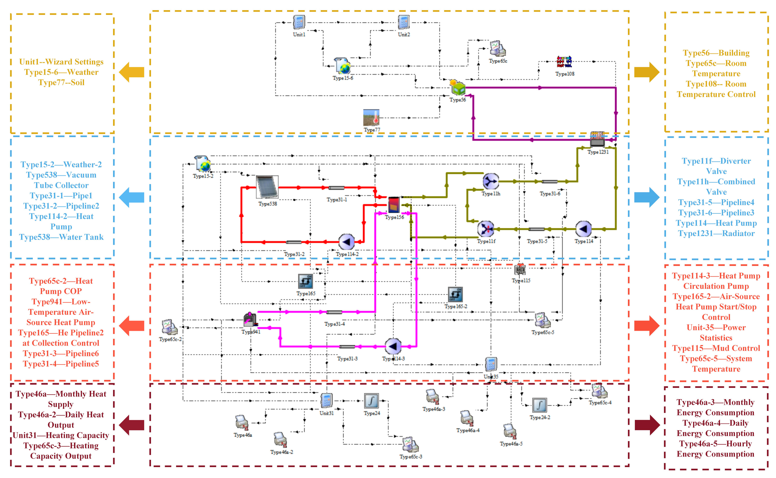
In order to realize the ultra-short-term time-series prediction for the problems of unstable heating load, uneven heat use and accurate heating in solar heating system, it is necessary to simulate the instantaneous dynamics of the whole system at the time of heating according to the connection relationship between the devices in the solar heating system, and complete the construction of the simulation model of the solar heating system in the TRNSYS platform. As shown in Figure 1:

As shown in Figure 1, the simulation model of solar heating system is simulated and analyzed for a regional building in Alar City, Xinjiang, with heating months from November 2024 to April 2025. Since the accuracy of the deep learning model’s ultra-short-term heating load prediction relies on high-resolution data support, the 7 min-level prediction used in this paper needs to be based on minute-level time-aligned load, meteorological and equipment operation datasets. Adequate data sample size combined with strictly synchronized temporal characteristics can effectively improve the model’s ability to capture building thermal dynamics and system transient processes. Therefore, the model has a maximum thermal load of 7.40 kw, an average thermal load of 3.95 kw, a simulation duration of 3600 h, and a simulation step size of 7 min.

The specific parameters of building models and equipment models within the system are established based on actual parameters sourced from a real solar heating system installed in a building in Alar City, Southern Xinjiang (4. Experimental Data Collection). The specific settings are described as follows:

(1)

Weather Data Reading Module (Weather (Type15)): This module reads standardized meteorological data (e.g., Typical Meteorological Year TMY2 format), providing hourly outdoor temperature, solar radiation, and other meteorological data for the simulation system. Typical meteorological data from Alar City, Southern Xinjiang, China, is selected as input for this module. (Data for this module was obtained using Metronome meteorological software (version 8.0.2) to derive specific weather conditions for Alar City, Southern Xinjiang.)

(2)

Vacuum Tube Collector Module (Type538): This module models the vacuum tube solar collector using Formulas (1)–(3) to simulate its heat collection process. The collector area is 7.4 m², with a flow rate of 35 kg/h·m² per unit area. The specific heat of the fluid medium is 3.53 kJ/kg·K. The collector efficiency parameters are 0a = 0.73 and 1a = 13.5.

(3)

Water Tank Module (Type 156). This module stratified storage tanks using Formulas (4)–(6) and connects to Type 538 to simulate the collector’s heat collection process. The tank is cylindrical with a volume of 2.4 m³ and height of 1 m, featuring a heat loss coefficient of 0.4 kJ/h·m²·K.

(4)

Auxiliary Heat Source Module Low-Temperature Air-Source Heat Pump (Type138). This module models the auxiliary heat source using Formula (7), with a fluid specific heat of 4.19 kJ/kg·K and a rated heating capacity of 14 kW.

(5)

Radiator Module (Type1231). This module models the radiator using Formulas (8) and (9), with a unit capacity parameter of 1.5 for cast iron radiators and a rated power of 0.2 kW.

(6)

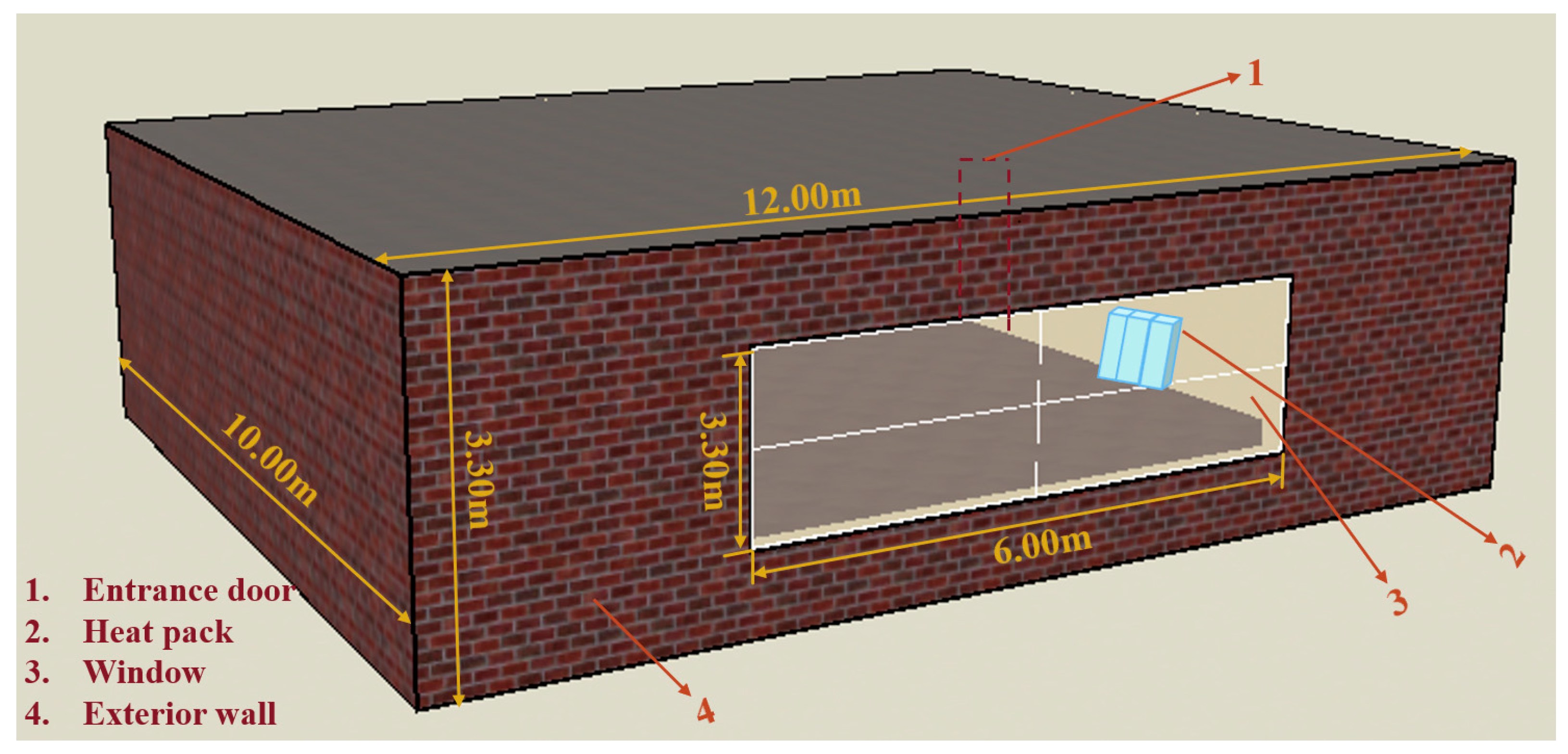
Building Module (Type56). As shown in Figure 2, the simulated building model has dimensions of 12 m (length), 10 m (width), and 3.3 m (height), with a volume of 396 m³ and a total floor area of 120 m². The building faces south. Exterior walls consist of cement mortar, rock wool, and autoclaved aerated concrete blocks. During the heating season, the indoor air temperature is maintained at 18 °C. The simulation parameters for the solar heating system are shown in

Table 1. Parameters of main components.

Part Name	Parameter	Numerical Value
Vacuum tube collector	Area/m2	7.4
	Inclination angle/°	50
Heat storage tank	Volume/m3	2.4
	Heat loss coefficient/kJ·h−1·m−2·K−1	0.4
Air source heat pump	Rated heat production/kw	14
	Rated power/kw	6.2
Cast iron radiator	Rated power/kw	0.2

.

Through the establishment of the above operation and regulation mathematical model and simulation model can be obtained solar heating system heating load data and solar heating system part of the main components of the parameters, and at the same time with the subsequent comparison and analysis of the experimental platform data, in order to achieve the conditions for the realization of the ultra-short-term time-series prediction, and to verify the effectiveness of the model of the solar heating system.

3. PSO-LSTM Model Building

3.1. LSTM Model Building

The LSTM model consists of multiple LSTM units connected chronologically, short-term memory is transmitted through the hidden layer of neighboring units, and long-term memory is transmitted through the network in chronological order. LSTM ensures information transmission through linear operation. The complete LSTM has three control units, input gate, output gate and forget gate, which are responsible for removing redundancy, updating data and transferring information downward (Cao et al., 2024 [19]). However, in the LSTM implicit layer, too many neurons will increase the computation, but the accuracy improvement is limited, and the hyper-parameters need to be reasonably adjusted, usually debugged or algorithmically optimized with 2n (Fang et al., 2024 [20]). As Figure 3 shows the structure of the long and short-term memory neural network:

LSTM is an improved recurrent neural network that specializes in processing time-series data with better stability and adaptability (Andi et al., 2025 [21]). When constructing an LSTM model, the number of neurons in the hidden layer and the learning rate are usually chosen based on experience or literature, and these two parameters directly affect the model accuracy and training speed. Particle swarm optimization (PSO) algorithm has significant advantages in optimizing neural network parameters due to its fast convergence and powerful search capability. In this paper, particle swarm algorithm is used to optimize the LSTM model (Qiu et al., 2025 [22]).

The LSTM algorithm employed in this study adopts a single-layer LSTM architecture to achieve single-step time-series forecasting. The detailed structure of each layer is as follows: (1) input layer; (2) first LSTM layer: 20 hidden units; (3) second LSTM layer: 20 hidden units; (4) fully connected layer: output dimension of 1; (5) regression output layer. Before integrating with PSO, optimization can be attempted through the following approaches: (1) network architecture: increasing the number of stacked LSTM layers, adding batch normalization layers before the fully connected layer, etc.; (2) hyperparameter tuning: appropriately adjusting the number of hidden units in LSTM, learning rate, and batch size; (3) and increasing the validation set.

3.2. Particle Swarm Optimization Algorithm

Particle Swarm Optimization Algorithm (PSO) is an evolutionary computing technique that originated from the study of the behavior of birds feeding in flocks (He et al., 2024 [23]). This behavior can be simply described as a group of birds that are searching for food and share a sole source of food in a specific area. By communicating with each other and sharing information about their respective locations, they enable the entire flock to congregate around the food.

Particle swarm algorithm (PSO), inspired by the flock behavior of birds, achieves an evolutionary process from disorder to order to solve the problem through information sharing and collaboration among individuals (Han et al., 2024 [24]). Each individual uses experience and group state to adjust its own state, the algorithm is easy to implement and insensitive to extreme conditions, and the failure of a single individual does not affect the overall operation. PSO is simple to operate, with fewer parameter requirements, and is widely used to improve the convergence speed and optimization ability, especially in function optimization and neural network training. Based on the advantages, this study employs the following parameterized design for the particle swarm optimization algorithm: the algorithm’s operational framework is primarily defined by specifying its fundamental parameters and the parameters of the parameter search space. The values for each parameter are listed in the

Table 2. PSO basic parameters and parameter search space table.

Parameters	Value
Population size	5
Maximum number of iterations	30
Optimization dimensions	4
Inertial weighting	0.8
Individual learning factor	1.5
Social learning factor	1.5
Learning rate (Parameter Search Space)	0.1
Maximum training rounds (Parameter Search Space)	200

below.

Simultaneously, to ensure the algorithm converges efficiently and reliably to the optimal solution, explicit convergence criteria were established. The convergence criteria for this algorithm are primarily defined through four convergence conditions and an adaptive convergence threshold. The four convergence conditions are the following: (1) reaching the maximum iteration count; (2) convergence of the fitness value; (3) stability of the optimal solution; (4) particle swarm clustering. The target conditions required for each criterion are detailed in the

Table 3. Convergence Criteria Conditions.

Convergence Condition	Target Requirements
Reached the maximum number of iterations
Fitness value convergence	Relative change is less than the threshold
Optimal solution stability	No significant improvements have been made over multiple generations.
Particle swarm optimality	All particle positions are close together

below.

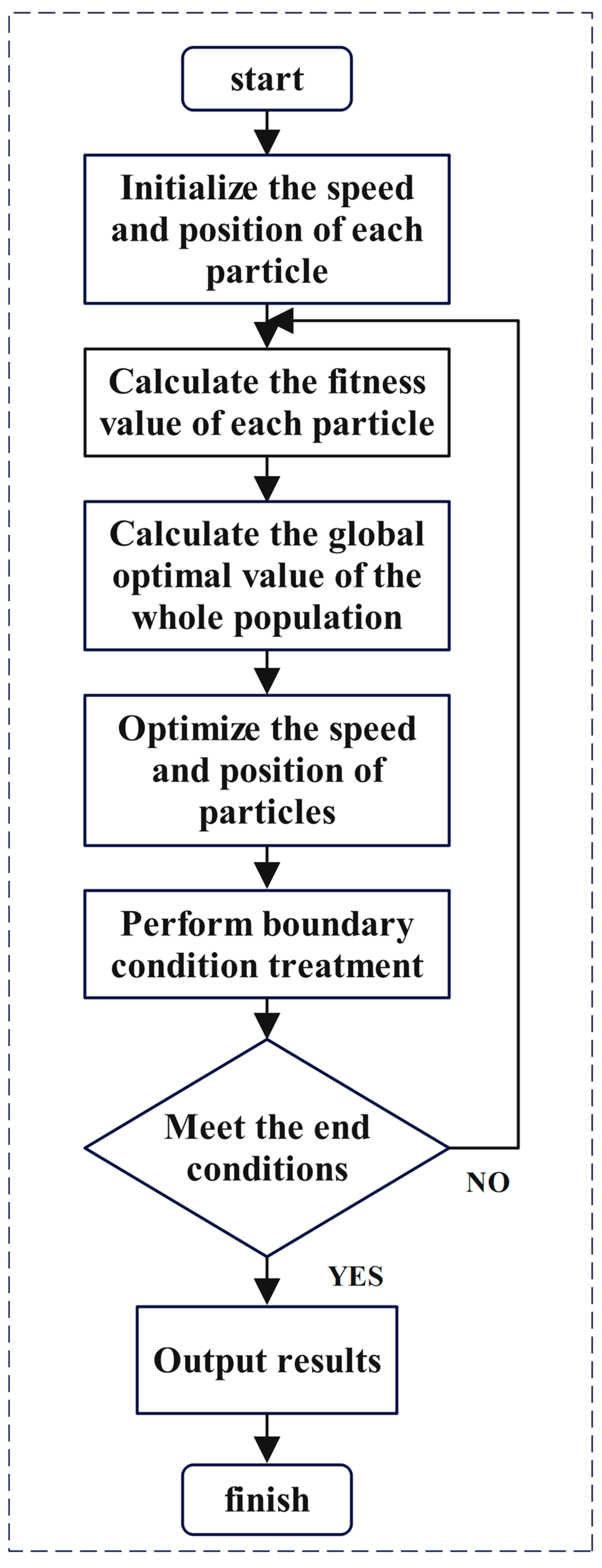
This comprehensive parameter and convergence design system effectively ensures the performance and efficiency of the algorithm when optimizing LSTM hyperparameters. As Figure 4 shows the particle swarm algorithm operation flow chart.

3.3. PSO-LSTM Model Construction

In this study, the existing heat load data are first carefully processed. The data contain information that needs to be organized and simplified through preprocessing, normalization, and other steps. Specifically, this includes normalization operations on the data to make the mean zero and minimize the variance (Thakur and Karmakar, 2025 [25]). Once this is done, the processed heat load historical data is entered into the established model as input values. The initialization of the model is a key aspect that determines the starting point of the entire training process. To ensure that the model can learn correctly and adapt to changes in the data, a stochastic approach is used in the initialization phase to generate the initial population as well as the associated parameters. This method can help the model start from scratch and gradually build a reasonable internal structure.

Based on this initialization framework, the hyperparameters for the PSO-optimized LSTM are as follows: (1) number of nodes in the first LSTM layer (L1); (2) number of nodes in the second LSTM layer (L2); (3) maximum training iterations (K); (4) initial learning rate (lr). As shown in the

Table 4. Optimized parameters.

Hyperparameters	Code Name (In the Code)
Number of nodes in the first LSTM layer	L1
Number of nodes in the second LSTM layer	L2
Maximum training rounds	K
Initial learning rate	lr

below.

Next, the training process of the ultra-short-term memory-based neural network is carried out using these carefully selected initialization parameters. Its network has a powerful memory function that can remember past input patterns to guide future behavior. The training process involves a large number of computations, and the network weights and parameters are continuously adjusted through repeated iterations with a view to achieving optimal adaptation. Ultimately, the fitness calculations are used to evaluate the network’s ability to predict new data as a means of determining the model’s suitability for solving a particular problem.

An in-depth analysis and comparison of the fitness of the particulate models is first conducted to establish a parameter optimization criterion using accuracy as a measure. To improve the learning efficiency of the model, the particle swarm algorithm (PSO) is introduced, which searches for the optimal solution by simulating the social behavior of biological populations in nature, and its core idea is to judge the individual’s strengths and weaknesses by evaluating the particle’s position in the search space, and then dynamically adjusting the particle’s velocity and position vectors in order to better approximate the globally optimal solution.

Under the PSO framework, the evaluation of new positions is not only used for the self-renewal of individuals but also takes into account the overall performance of the population. This means that each particle is not just isolated in its optimality seeking behavior but seeks common progress at the population level. Based on a pre-set maximum number of iterations, the system determines whether the current iteration has reached its goal, and if not, it restarts training as a way to ensure that the algorithm is able to continuously explore new possibilities.

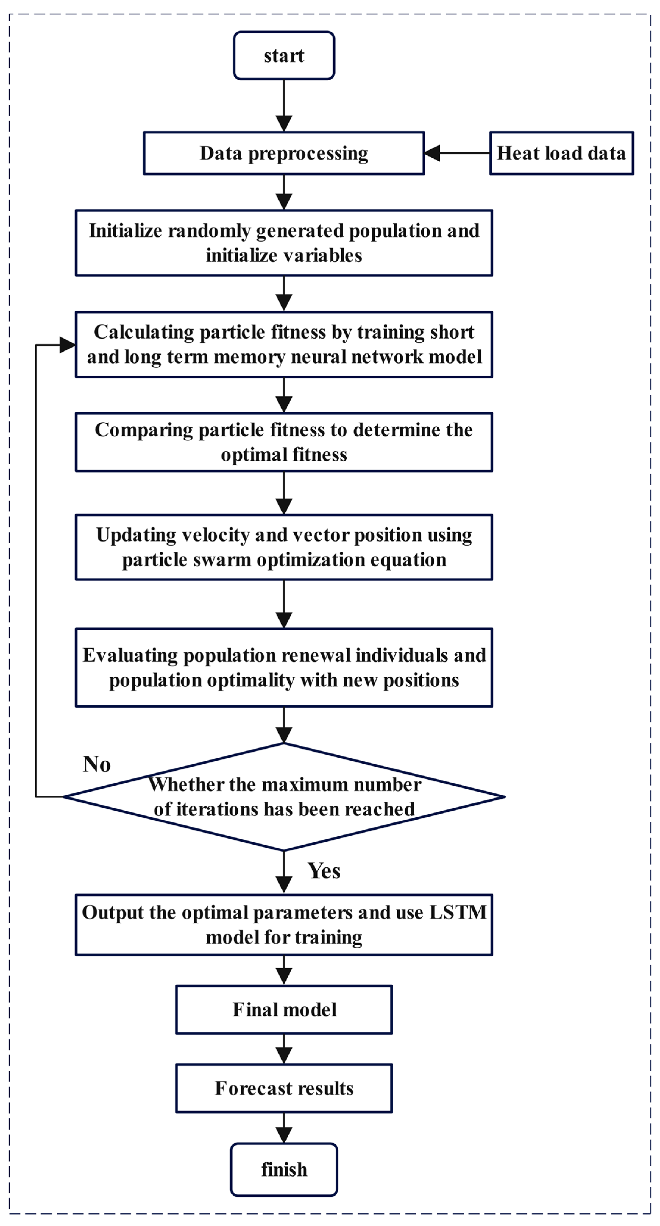
After several rounds of iterations, an optimal parameter configuration scheme can be determined when the particle swarm returns to a fixed point. At this point, the selected optimal parameters are further trained using a long-term memory neural network (LSTM). During the training process, the prediction effect of the LSTM model is closely monitored to ensure that it has good performance and reliability in real application scenarios. In this way, better models can be obtained to support various scientific research and engineering practices. Figure 5 shows the particle swarm algorithm optimization LSTM flow chart.

4. Experimental Data Acquisition

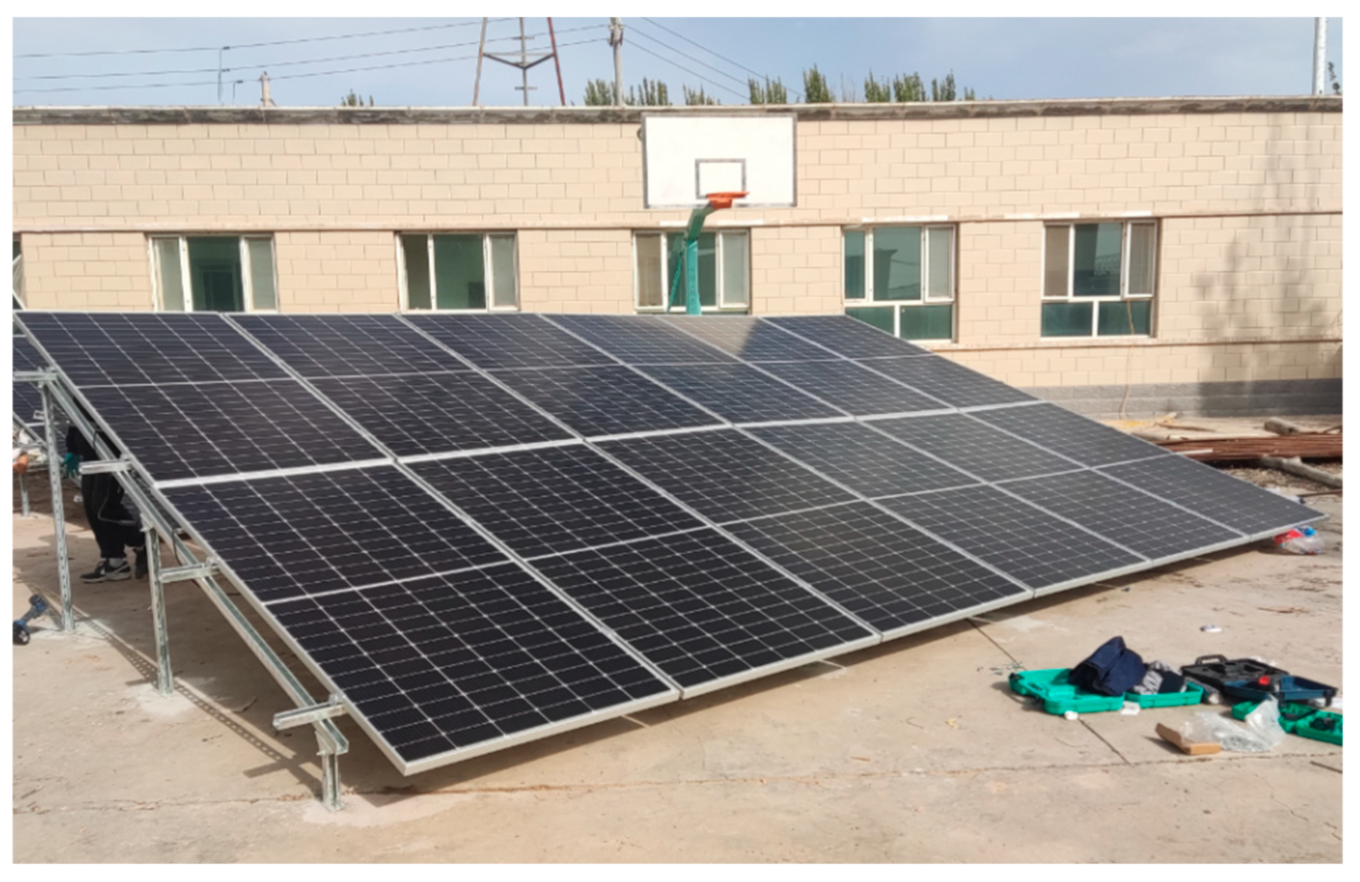
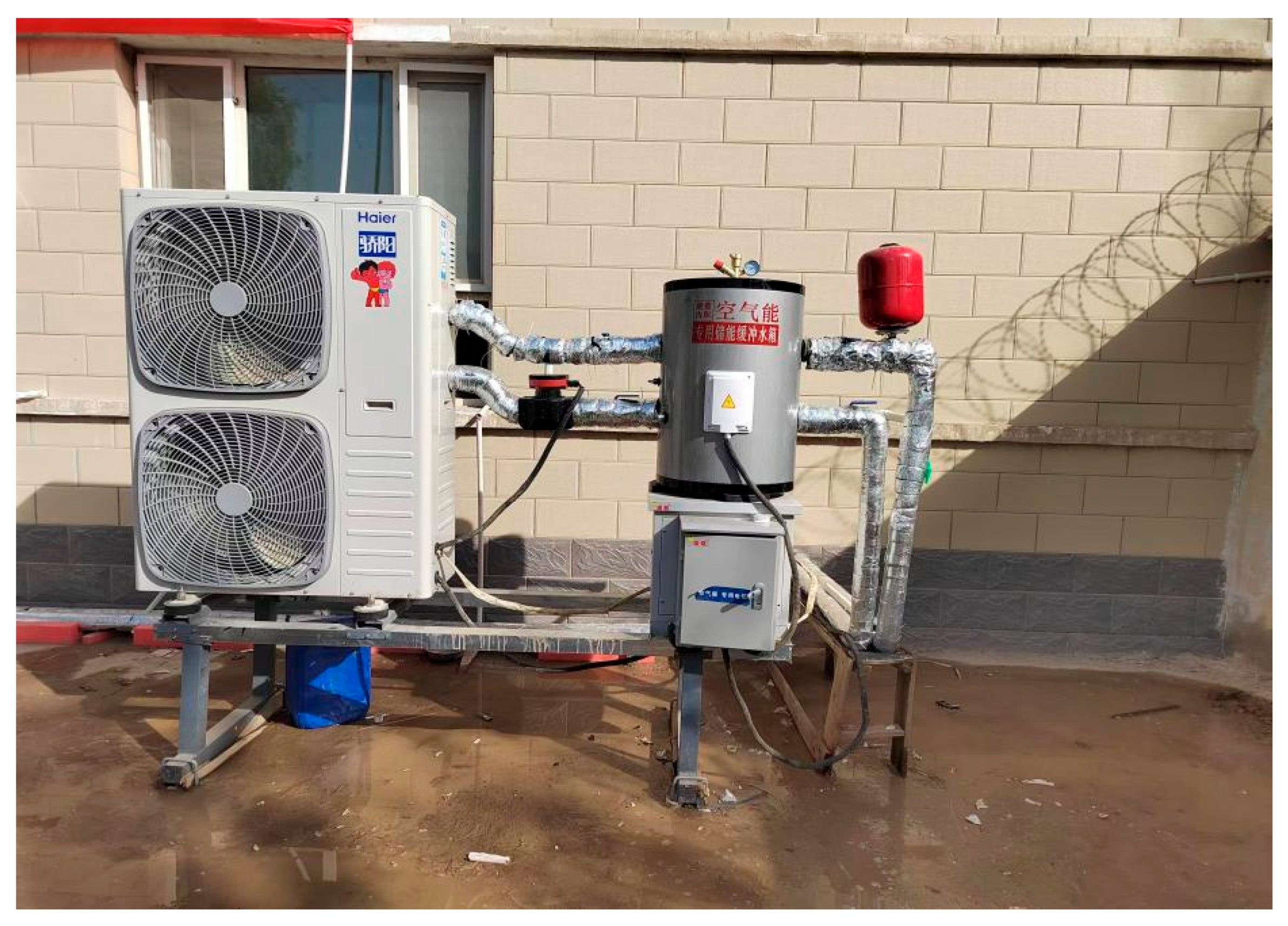
This study conducted equipment calculations and selection for a solar heating system in a specific area of Alar City, Southern Xinjiang, and established a corresponding experimental platform. Actual operational data were collected through on-site testing to construct an experimental dataset, which was used to validate the accuracy of the simulation platform. Comparative analysis between experimental data and simulation results demonstrated that the simulation platform’s output data were largely consistent with measured data, confirming the reliability of the simulation model.

The dataset selected for this study comprises heating load data from 11 November 2024, to 1 January 2025. Sampling intervals were set at 7 min intervals, yielding approximately 205 samples per day and exceeding 12,000 data rows. Units are in degrees Celsius (°C). Recorded data include indoor and outdoor temperatures, radiator temperatures, collector temperatures, and average water tank temperatures.

This period encompasses the entire heating season, representing the coldest and highest heating demand period in southern Xinjiang. The process spans from initial cooling to severe cold, covering the most challenging operating conditions the model must handle.

The study includes diverse weather patterns: multiple stable clear days (testing the solar sufficiency model) alongside extreme and transitional periods (e.g., snowfall) (evaluating system performance under severe disturbances). It is important to note that no single climate model was used for validation.

Given the high sampling frequency, the 7 min interval over three months provided a substantial volume of valid data. This ample dataset was sufficient for training and validating the deep learning model. Figure 6 and Figure 7 illustrate the field-deployed experimental platform.

Through the experimental platform, we obtained a series of relevant datasets. Figure 8 illustrates indoor and outdoor temperature variations simulated using the Origin platform, while

Table 5. Special Weather Data.

Date	Weather	Average Outdoor Temperature °C	Average Indoor Temperature °C	Average Radiator Supply Temperature °C	Average Water Tank Temperature °C	Average Collector Inlet Temperature °C	Average Collector Outlet Temperature °C
11 November 2024	Sunny	17.6	19.2	40.7	45	38.6	35.6
18 November 2024	Cloudy day	16.5	18.9	39.4	45	42.2	40.7
23 November 2024	cloudy	17.2	18.1	38.5	45	41.6	37.6
28 November 2024	Aeolian sand	15.9	18.3	38.7	45	39.8	38.8
18 December 2024	heavy snow	−17.5	19.4	39.8	44	37.7	36.7
21 December 2024	Light snow	−17.1	19.1	39.8	44	39.7	38.6
23 December 2024	Light snow	−18.1	18.9	40.2	45	41.2	37.8

lists partial temperature data achievable by the solar heating system under specific weather conditions. This information holds significant importance for analyzing system performance, optimizing designs, and enhancing energy utilization efficiency.

The graph clearly shows that indoor and outdoor temperatures exhibit distinct fluctuation patterns across different time periods. These fluctuations not only reflect the impact of external environmental factors—such as solar radiation intensity and ambient temperature—on system performance but also reveal changes in the system’s operational state. By analyzing this data, we can gain a more accurate understanding of the system’s operational efficiency under various conditions, providing robust support for subsequent optimization designs. Table 5 presents selected data from specific weather events.

4.1. Data Preprocessing

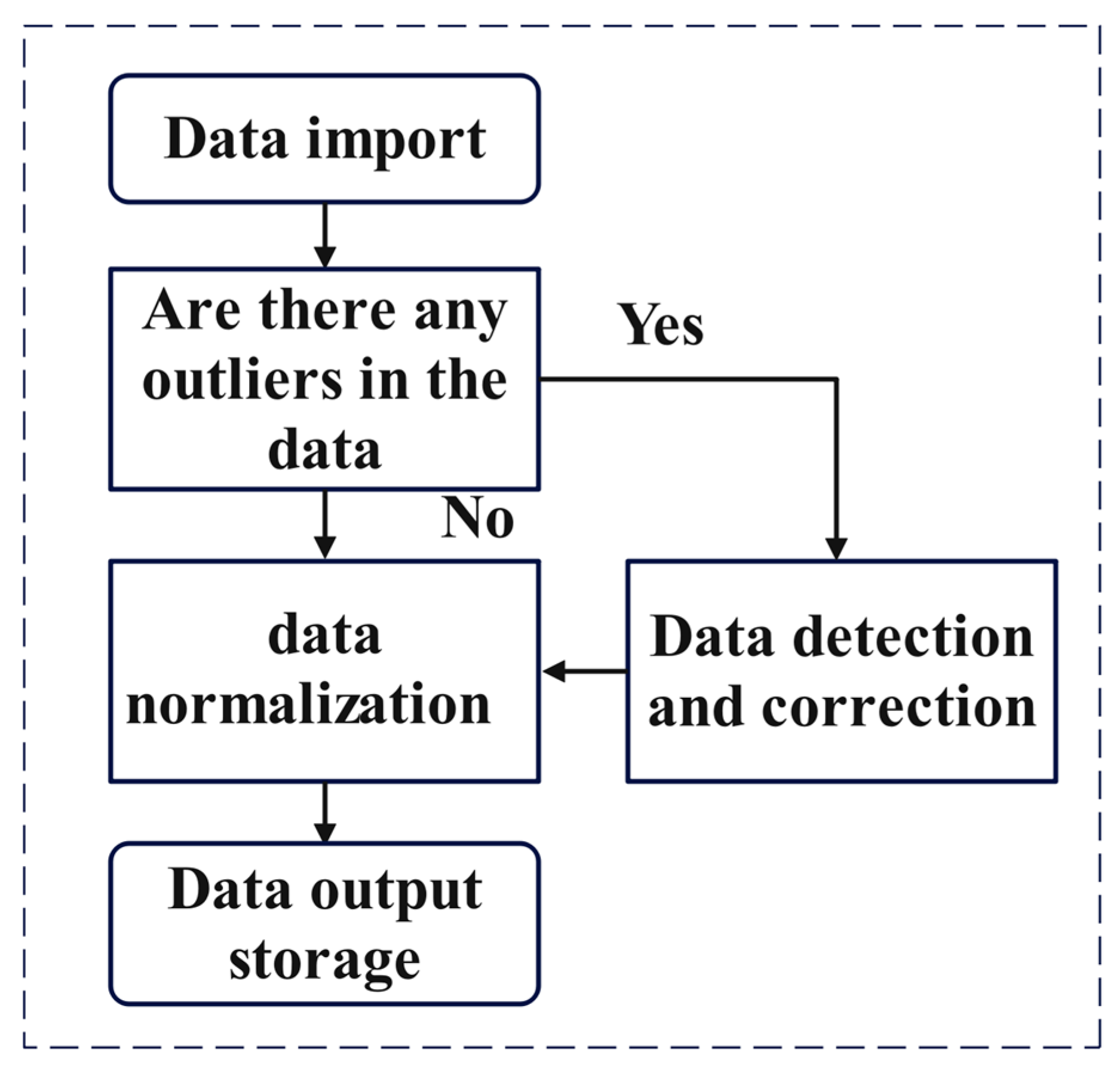
Data preprocessing is a key step in data analysis and modeling, aiming to improve data quality, reduce noise and outliers, and fill in missing data by cleaning, transforming, and normalizing the data, so as to enhance the accuracy and reliability of the model. Indispensable to the load forecasting research process is the preprocessing of raw data. The load data preprocessing process is shown in Figure 9:

4.2. Data Normalization

Data normalization is a method of processing the input data into values between 0 and 1. In this way, it can effectively reduce the input spatial range, accelerate the convergence speed of the model, and help to prevent the occurrence of gradient explosion or disappearance phenomenon, so as to improve the prediction accuracy and facilitate the subsequent data analysis and processing. In this paper, the minimum–maximum (min–max) normalization method is used to achieve the linear transformation of the data, which is conducted as follows: for each eigenvalue, it is subtracted from the minimum value of the eigenvalue in all the samples, and then divided by the difference between the maximum value of the eigenvalue and the minimum value of the eigenvalue. This method ensures that all eigenvalues are mapped into the [0, 1] interval. The formula for this is as follows:

$$L={\displaystyle \frac{L_i-L_{\mathit{min}}}{L_{\mathit{max}}-L_{\mathit{min}}}}$$

(12)

Style: $L_i$—time point value; $L_{\mathit{min}}$—sample minimum, $L_{\mathit{max}}$—sample maximum; $L$—sample normalized value.

4.3. Model Evaluation Indicators

Evaluation metrics can not only directly reflect the strengths and weaknesses of the model prediction results but also be used to compare the accuracy between different models. In this study, we choose three main evaluation metrics to measure the model performance: the coefficient of determination (R²), the root means square error (RMSE), the mean absolute error (MAE), and the mean absolute percentage error (MAPE). All three metrics can be used to quantify the degree of difference between predicted and actual values (Yang et al., 2024 [26]).

The coefficient of determination (R²) is calculated by subtracting the sum of the squared differences of all predicted values from the mean of the true values from 1 and dividing by the sum of the squared differences of all true values from their means. This metric is used to measure how well the model fits. Typically, the value of R² lies between 0 and 1. The closer the value is to 1, the better the model performs. The formula is shown below:

$$R^2=1-{\displaystyle \frac{{\sum }_{i=1}^n{\left(y_i-\overline{y_i}\right)}^2}{{\sum }_{i=1}^n{\left(y_i-\overline{y_i}\right)}^2}}$$

(13)

Style: $y_i$—predicted value; $y_i$—true value; $\overline{y_i}$—mean of true value; $n$—predicted data length.

The Root Mean Square Error (RMSE) is a common measure of the difference between predicted values and actual observations. Specifically, it is calculated as the sum of the squares of the differences between all predicted values and their corresponding true values divided by the number of predicted data points, and then the square root is taken. This metric is particularly sensitive to extreme deviations present in the data set, as the squaring operation amplifies the effect of larger errors. Thus, the RMSE not only reflects the overall predictive accuracy of the model, but also effectively points out possible deficiencies in the model’s handling of particular samples. By reducing the RMSE value, the model’s ability to generalize unknown data and stability can be improved. The formula is as follows:

$$\mathrm{RMSE}=\sqrt{{\displaystyle \frac{{\sum }_{i=1}^n{\left(y_i-y_i\right)}^2}{n}}}$$

(14)

Style: $y_i$—predicted value; $y_i$—true value; $\overline{y_i}$—mean of true value; $n$—predicted data length.

The Mean Absolute Error (MAE) is an important measure of a model’s prediction performance, which is calculated as the sum of the absolute values of the differences between all predicted values and the corresponding true values, divided by the number of predicted data points. The MAE is an intuitive reflection of the model’s level of prediction error in its entirety, as it takes into account the magnitude of each individual error without regard to its directionality. It is particularly straightforward and effective when it comes to the costs or losses that may be incurred in real-world applications. A lower MAE value indicates that the model has a higher level of predictive accuracy and reliability. The formula for this is as follows:

$$\mathrm{MAE}={\displaystyle \frac{{\sum }_{i=1}^n\left|y_i-y_i\right|}{n}}$$

(15)

Style: $y_i$—predicted value; $y_i$—true value; $\overline{y_i}$—mean of true value; $n$—predicted data length.

MAPE average absolute percentage error is normalized for each point, in the form of a percentage of the performance and the true value of the gap, and MAPE can effectively reduce the impact of outliers, the value of the range of (0,+∞), the smaller the value of the MAPE error, indicating that the model prediction accuracy is higher. The formula is as follows:

$$\mathrm{MAPE}={\displaystyle \frac{100\%}{n}}\sum _{i=1}^n\left|{\displaystyle \frac{y_i-\widehat{y}}{y_i}}\right|$$

(16)

Style: $y_i$—predicted value; $y_i$—true value; $\overline{y_i}$—mean of true value; $n$—predicted data length.

5. Analysis of Experimental Results

Since the focus of this paper is on the study of ultra-short-term heating load prediction for stable weather conditions and the environment, the model selection in this paper only considers the comparison of indoor temperature, heat collection and system energy consumption.

The data parameters and the dataset in Section 4 are used for the experiments. The dataset comprises 7 min interval temperature load values recorded every 24 h from 1 November to 10 December, serving as the training set. This set is randomly divided into training and testing sets at a 7:3 ratio. The trained model predicts temperature load values from 11 December to 1 January of the following year based on the temperature load values recorded on 10 December. The initial data starts from 24 h. The implementation is written in MATLAB R2023a language with input variable dimension of 3 and output variable dimension of 1.

In order to compare the prediction effect of the optimized model, an LSTM neural network model was built for the load dataset. The data from 1 November to 10 December is used as a sample to train the model and the temperature load data from 11 December to 1 January is predicted to verify the accuracy with an input dimension of 3 and an output dimension of 1.

Input feature dimensions include three inputs: indoor temperature, heat collection, and system energy consumption (The time points −1, −2, −3, etc., in the table below represent recorded time points every 7 min). Specific details are shown in the

Table 6. Input feature dimensions.

Time Point	Feature 1: Indoor Temperature (°C)	Feature 2: Heat Collection (KW)	Feature 3: System Energy Consumption (KW/h)
11 December 2024 (1)	18	1.11	0.53
11 December 2024 (2)	17.97	1.92	0.79
11 December 2024 (3)	17.91	2.57	1.58
11 December 2024 (4)	17.85	3.08	2.37
11 December 2024 (5)	17.8	3.50	3.16
11 December 2024 (6)	17.75	3.87	3.95
11 December 2024 (7)	17.7	3.87	4.75
11 December 2024 (8)	17.6	3.87	5.54
11 December 2024 (9)	17.62	3.87	6.34
11 December 2024 (10)	17.58	4.75	7.13
11 December 2024 (11)	17.55	5.44	7.93
11 December 2024 (12)	17.51	5.97	8.73
11 December 2024 (13)	17.48	6.37	9.53
11 December 2024 (14)	17.45	6.37	10.33

below.

This study employs Pearson’s correlation coefficient to compare the strength of linear relationships between various input features and the system heating load. Analysis of continuous time-series data from operational conditions yielded the following correlations. Specific parameters are shown in

Table 7. Input feature dimensions.

Characteristic Variables	Heating Load	Indoor Temperature	Heat Collection	System Energy Consumption
Heating Load	1.000	−0.998	0.983	0.955
Indoor Temperature	−0.99	1.000	−0.974	−0.998
Heat Collection	0.983	−0.974	1.000	0.983
System Energy Consumption	0.995	−0.998	0.983	1.000

.

The results indicate a negative correlation coefficient of −0.998 between heating load and indoor temperature. This demonstrates that a slight decrease in indoor temperature (e.g., from 18.0 °C to 17.7 °C) corresponds to a significant increase in heating load. This aligns with the physical principle in building thermodynamics that wall heat loss is proportional to the indoor−outdoor temperature difference. This characteristic most directly and sensitively reflects the thermal demand at the user end.

A significant positive correlation exists between heating load and energy consumption, reaching 0.995. This reflects the principle of energy conservation, where the energy input into the system ultimately converts into thermal output, serving as the most direct driving force.

A high positive correlation of 0.983 exists between the collection efficiency and heating load. This indicates that solar energy and auxiliary heating are mutually coordinated during the selected data period. The improvement in collection efficiency stems from both increased solar radiation intensity and the effective utilization of renewable energy.

The important parameters of LSTM are shown in

Table 8. LSTM parameter settings.

Parameter	Numerical Value	Parameter	Numerical Value
Learning rate	0.005	Number of iterations	20
Gradient descent threshold	1	Input feature dimension	3
Number of hidden units	40	Output feature dimension	1

.

In PSO-LSTM, the parameters to be set are acceleration coefficient C₁C₂, population size, number of iterations, number of evolutions and speed range.

Particle swarm size M: represents the total number of particles contained in the particle population of the particle swarm algorithm, the total number of particles is not the better, but needs to be decided according to the actual problem to be dealt with. Increasing the total number of particles can improve the optimization effect, but too large a total number of particles will slow down the optimization speed. Reducing the total number of particles can shorten the optimization time, but too small a total number of particles will lead to premature convergence and thus not get the optimization result. In this study, the particle population size is selected as 5.

Learning factor: It is used to regulate the individual and population searching ability and the size of learning amplitude to guide the particles to move towards the global optimal position. Among them, C₁ determines the next-generation forward direction and forward speed of individual particles, and C₂ determines the forward direction and forward speed of the whole population. Generally, C₁ = C₂ is set, and C₁ = C₂ = 1.5 is usually chosen, so that the population experience and individual experience have the same important influence, making the final optimal solution more accurate.

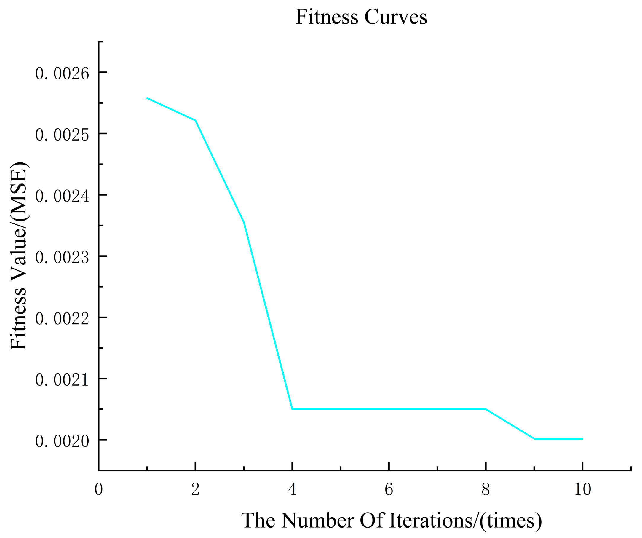
Maximum number of iterations: This parameter is determined by the specific experiment, if the number of iterations is set too large, the algorithm has not stopped when the optimal result has been found, which will cause a waste of time and memory. If the number of iterations is set too small, the algorithm stops when the search for the optimum is not sufficient, resulting in not finding the global optimum. Usually, 20–100 iterations are chosen, and in this study, the maximum number of iterations is chosen to be 20 through several trials.

After the PSO model optimization parameters: the learning rate is 0.0062; the number of hidden units is 260. The parameter settings are shown in

Table 9. PSO-LSTM parameter settings.

Parameter	Numerical Value	Parameter	Numerical Value
Evolution number	10	Speed range	[1, 4]
Population size	5	C1	1.5
Number of iterations	30	C2	1.5

.

The fitness curve is shown in Figure 10:

To enhance the accuracy of the results, simulation experiments were conducted using the two models to evaluate indoor temperature, heat collection, and energy consumption under both clear-weather and special-weather conditions. The error evaluation metrics from both models were adopted as the outcome.

5.1. Comparison Analysis of Indoor Temperatures on Sunny Days

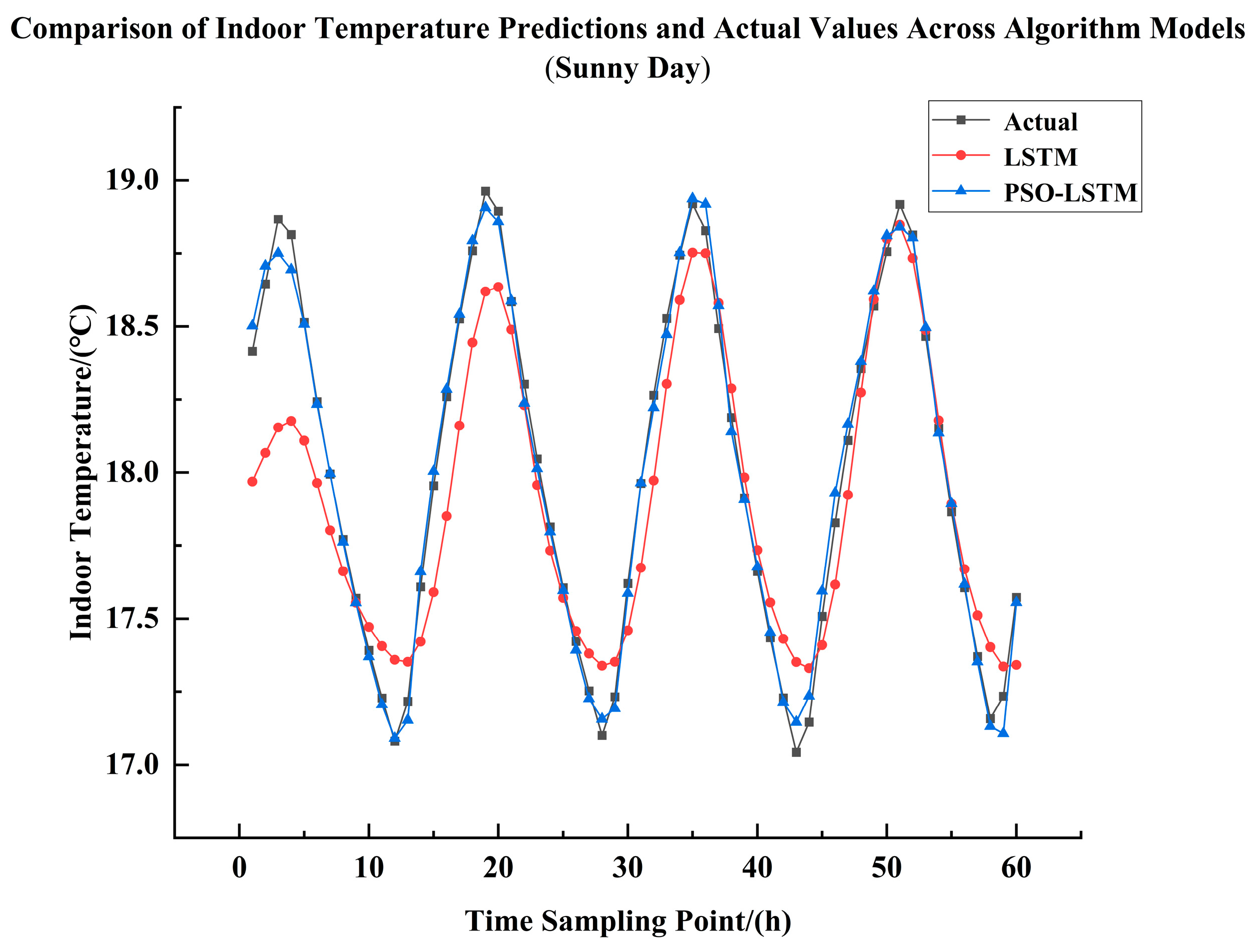
Simulation Experiment on Indoor Temperature on Sunny Days, it is evident from Figure 11 and

Table 10. Comparison of error evaluation indicators.

Model Type	R2	RMSE	MAE	MAPE%
LSTM	0.82272	0.24885	0.19606	1.0842%
PSO-LSTM	0.98427	0.07413	0.05509	0.3047%

that the PSO-LSTM neural network achieves a higher degree of curve fitting compared to the LSTM neural network. That is to say, the PSO-LSTM model predicts better than the LSTM model, which can be seen in the above table: the R² of the PSO-LSTM model is improved by 0.17 than that of the LSTM model, and at the same time, the PSO -LSTM model reduces RMSE by 0.174 °C and MAE by 0.141 °C than the LSTM model; in relative comparison, R² improves by 16.5%, RMSE reduces by 70.2%, MAE reduces by 72%, and MAPE reduces by 71.9%.

5.2. Comparative Analysis of Solar Heat Collection on Clear Days

Simulation Experiment on Solar Heat Collection in Clear Weather, it is obvious that the PSO-LSTM neural network fits the curve better than the LSTM neural network through Figure 12 and

Table 11. Comparison of error evaluation indicators.

Model Type	R2	RMSE	MAE	MAPE%
LSTM	0.17686	13.3129	10.02	15.0913%
PSO-LSTM	0.98082	2.032	1.6265	3.1302%

, which can be seen from the Table 11: the R² of the PSO-LSTM model is improved by 0.81 compared to that of the LSTM model, and at the same time, the RMSE of the PSO-LSTM model is reduced by 11.28 KW compared to that of the LSTM model; MAE is reduced by 8.39 KW; in relative comparison, R² is improved by 82%, RMSE is reduced by 84.8%, MAE is reduced by 83.8%, and MAPE is reduced by 79.3%.

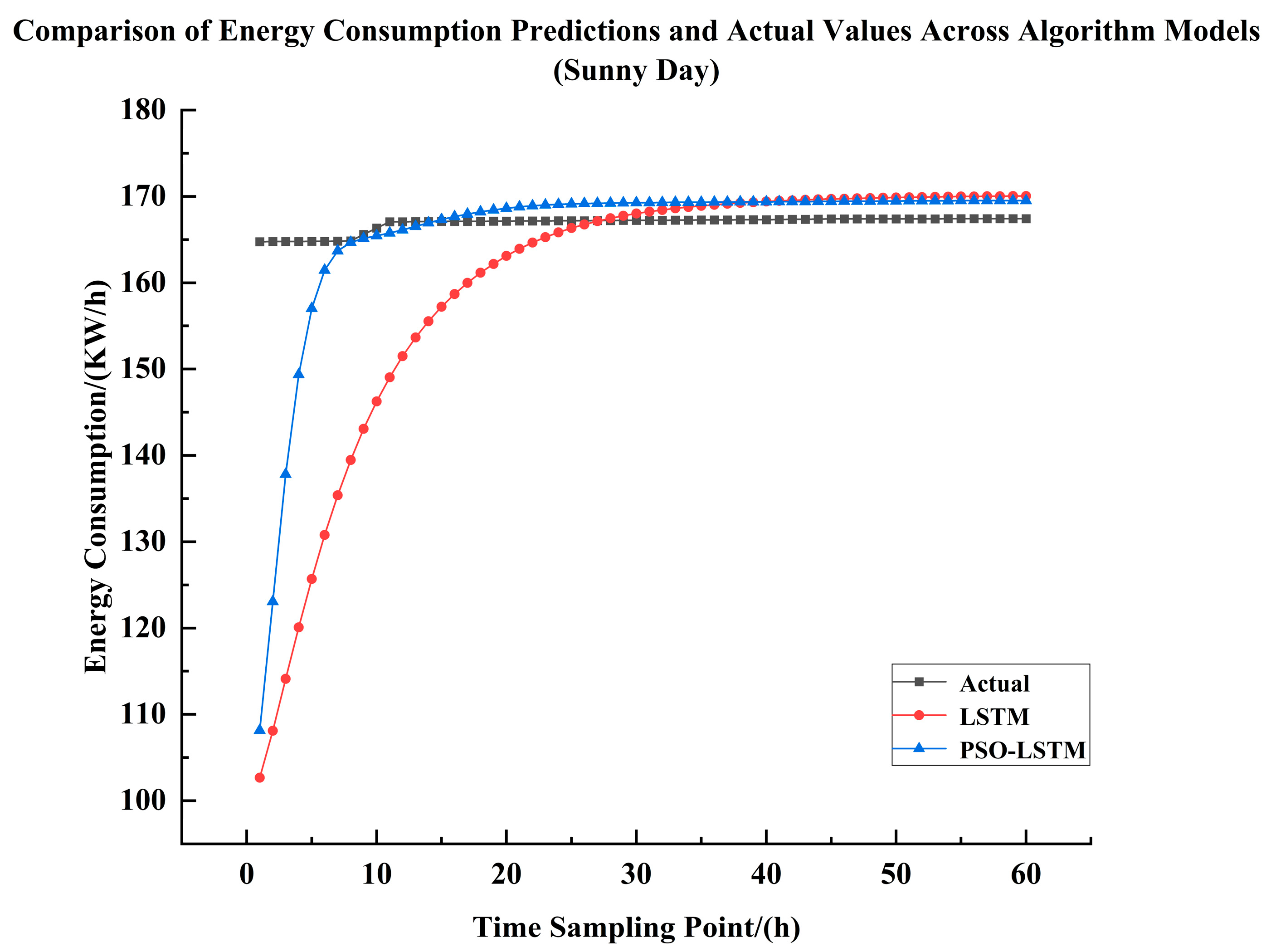
5.3. Comparative Analysis of Energy Consumption in Sunny Weather Systems

System Energy Consumption Simulation Experiment for Sunny Days, it is obvious that the PSO-LSTM neural network has a higher degree of curve fitting than the LSTM neural network through Figure 13 and

Table 12. Comparison of error evaluation indicators.

Model Type	R2	RMSE	MAE	MAPE%
LSTM	0.84249	12.9477	10.404	5.7386%
PSO-LSTM	0.87031	3.7575	2.0351	1.1537%

, which can be seen in the Table 12: the PSO-LSTM model has an increase of 0.03 in R² compared to the LSTM model, and at the same time, the PSO-LSTM model reduces the RMSE by 9.19 KW/h compared to the LSTM model; MAE is reduced by 8.369 KW/h; in relative comparison, R² is improved by 3.3%, RMSE is reduced by 70.8%, MAE is reduced by 80.5%, and MAPE is reduced by 79.9%.

5.4. Indoor Temperature Comparison Analysis During Snowy Weather

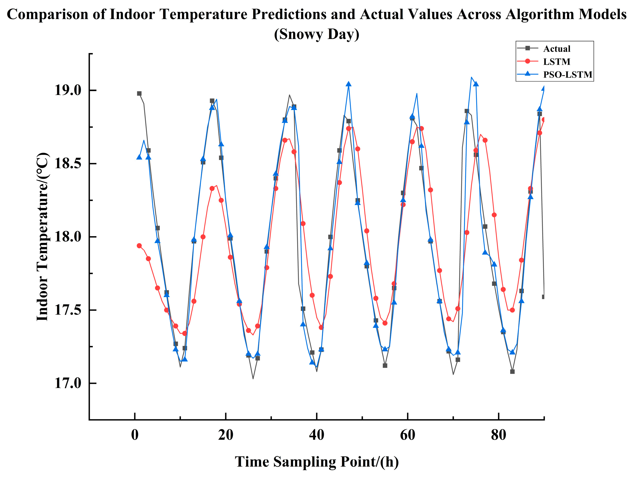
Regarding the indoor temperature simulation experiment during heavy snowfall, Figure 14 and

Table 13. Comparison of error evaluation indicators.

Model Type	R2	RMSE	MAE	MAPE%
LSTM	0.6104	0.37566	0.27714	1.5533%
PSO-LSTM	0.85132	0.23207	0.11703	0.65135%

clearly demonstrate that the PSO-LSTM neural network achieves superior curve fitting compared to the LSTM neural network. This indicates that the PSO-LSTM model delivers better prediction performance than the LSTM model. As shown in the Table 13: the PSO-LSTM model improves the R² value by 0.25 compared to the LSTM model, while simultaneously reducing the RMSE by 0.143 °C; the Mean Absolute Error (MAE) decreased by 0.16 °C; relatively speaking, R² increased by 28.3%, RMSE decreased by 38.2%, MAE decreased by 57.8%, and MAPE decreased by 58%.

5.5. Comparative Analysis of Heat Collection in Snowy Conditions

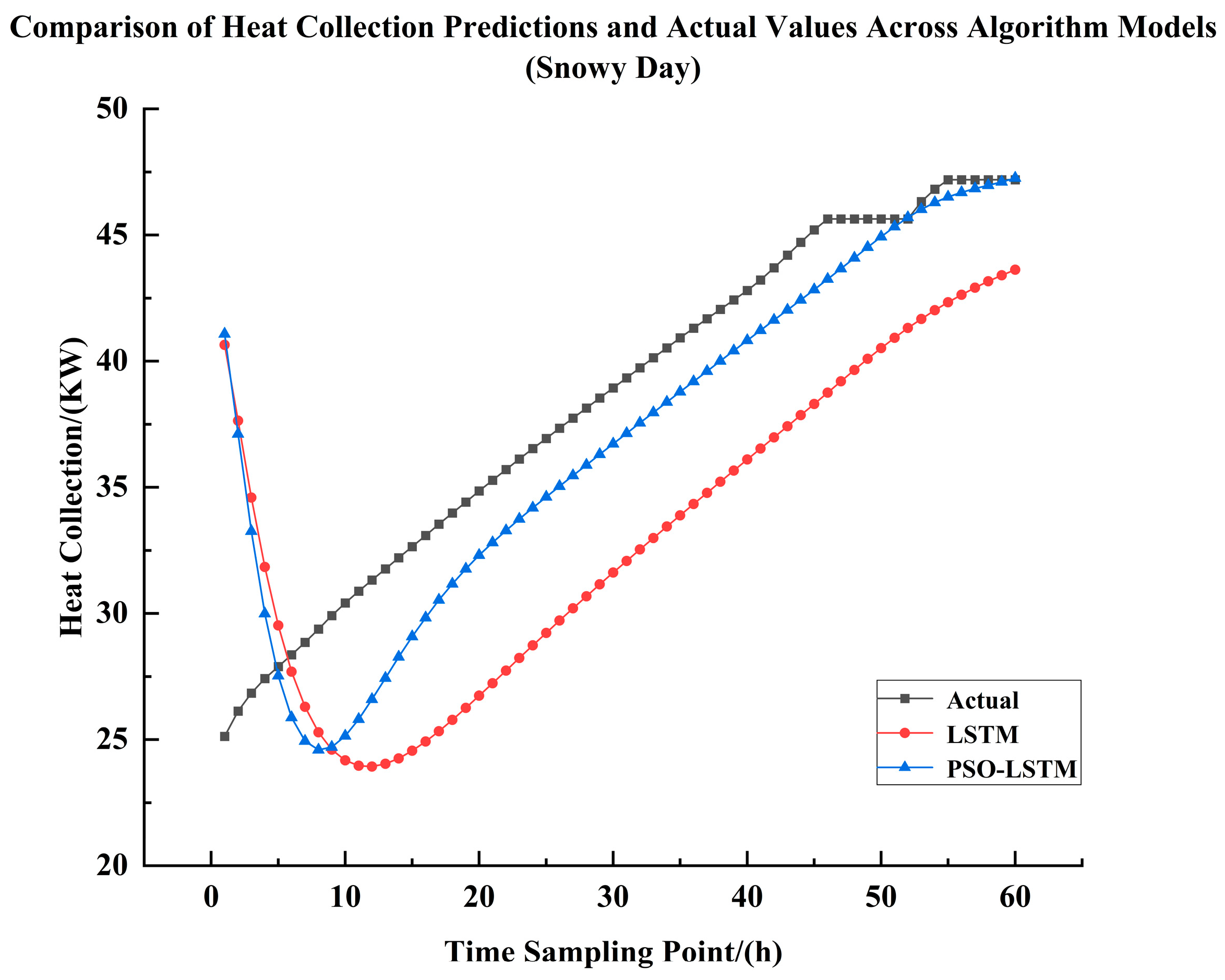
Regarding the simulation experiment on heat collection during heavy snowfall, Figure 15 and

Table 14. Comparison of Error Evaluation Indicators.

Model Type	R2	RMSE	MAE	MAPE%
LSTM	0.12878	49.673	38.0686	6.1521%
PSO-LSTM	0.96421	10.0347	3.4251	0.60018%

clearly demonstrate that the PSO-LSTM neural network achieves superior curve fitting compared to the LSTM neural network. As shown in the Table 14: the PSO-LSTM model improves the R² value by 0.84 over the LSTM model, while simultaneously reducing the RMSE by 39.6 KW. MAE decreased by 34.64 KW. In relative terms, R² increased by 86.7%, RMSE decreased by 79.8%, MAE decreased by 91.1%, and MAPE decreased by 90.3%.

5.6. Snowy Weather System Energy Consumption Comparison Analysis

Regarding the simulation experiment on system energy consumption during heavy snow fall, Figure 16 and

Table 15. Comparison of Error Evaluation Indicators.

Model Type	R2	RMSE	MAE	MAPE%
LSTM	0.31139	42.8587	29.9515	2.0759%
PSO-LSTM	0.96634	7.9603	3.8378	0.26929%

clearly demonstrate that the PSO-LSTM neural network achieves superior curve fitting compared to the LSTM neural network. As shown in the Table 15: the PSO-LSTM model improves the R² value by 0.65 compared to the LSTM model, while simultaneously reducing the RMSE by 34.89 kW/h. MAE decreased by 26.12 kW/h. In relative terms, R² improved by 67.8%, RMSE decreased by 81.5%, MAE decreased by 87.2%, and MAPE decreased by 87.1%.

5.7. Statistical Significance Test Analysis of LSTM and PSO-LSTM

To demonstrate the stability and reliability of the model, this study will conduct significant tests, specifically as follows:

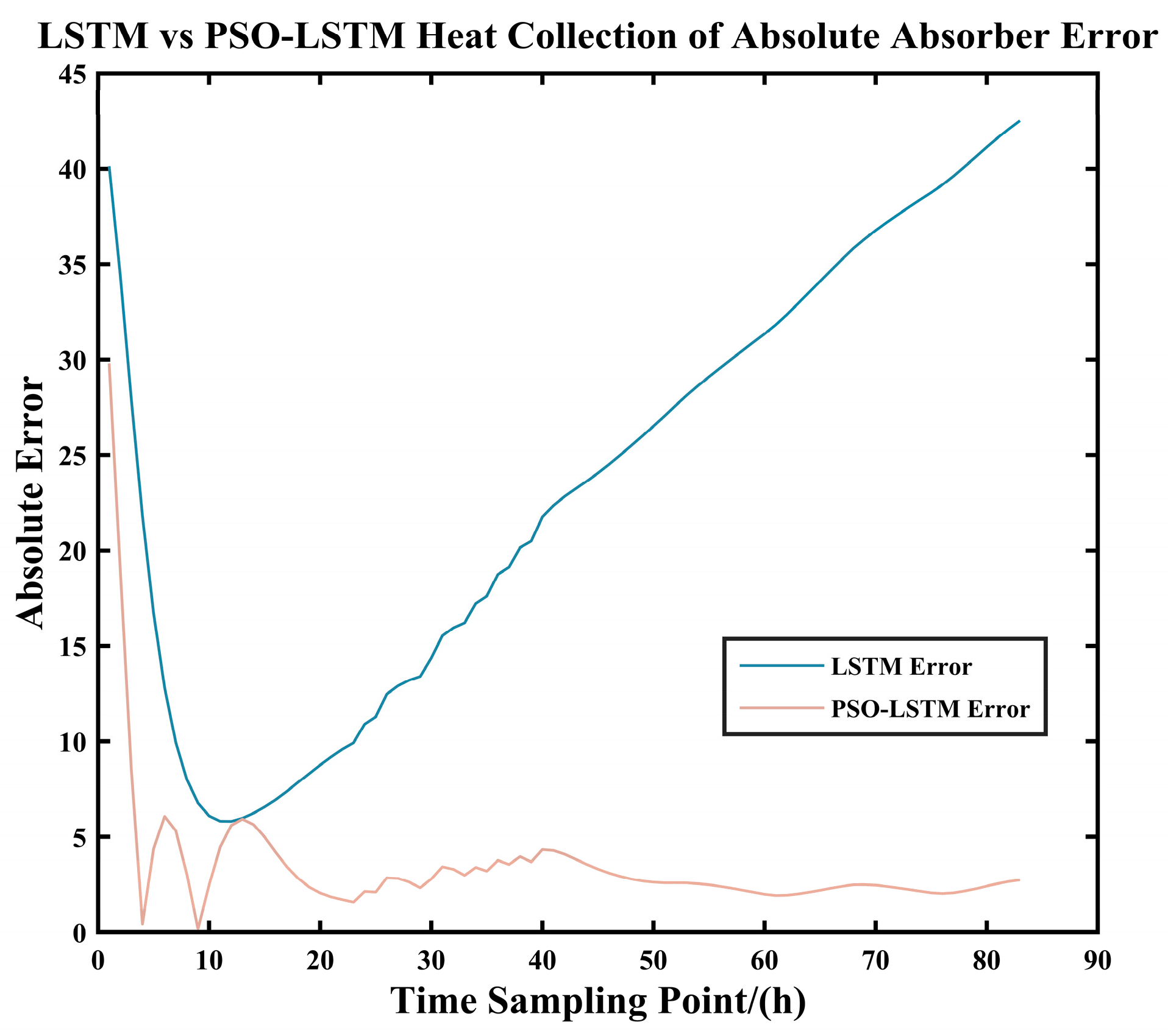
As shown in Figure 17 and Figure 18 and

Table 16. LSTM vs. PSO-LSTM Significance Analysis Comparison of Heat Collection.

		LSTM	PSO-LSTM	Improvement
Basic Statistical Information	Sample size	166	166
	Mean error	19.36	2.93	+84.87%
	Standard Deviation of Error	11.47	3.51	+69.41%
	Median error	18.75	2.46	+86.87%
Performance Metrics	RMSE	22.48	4.56	+79.71%
	MAE	19.36	2.93	+84.87%
	MAPE	2.85	0.44	+84.71%

RMSE: Root Mean Squared Error; MAE: Mean Absolute Error; MAPE: Average Absolute Percentage Error.

, after predicting the solar collection heat for the same 166 sample points, the PSO-LSTM model demonstrated significantly superior prediction error and model evaluation metrics compared to the LSTM model. The PSO-optimized LSTM achieved improvement rates of up to 84.87% for all metrics, with the minimum improvement rate reaching 69.41%. This demonstrates that the PSO algorithm significantly enhances the solar heat collection prediction capabilities of the LSTM model.

As shown in the

Table 17. Statistical Significance Test (α = 0.05).

Type	LSTM	PSO-LSTM
Test for Normality of Error	p = 0.0175 *	p = 0.001 **
Wilcoxon Signed-rank Test	p = 0 ***	Cohen’s d Effect Size = 1.94 (big)

* denotes significant, ** denotes highly significant, and *** denotes extremely significant.

, the Wilcoxon Signed-Rank Test was employed because the errors did not follow a normal distribution. Additionally, the table indicates a significant difference (p < 0.05) in the prediction of heat collection between the two models. The LSTM model optimized by PSO demonstrated a significant improvement in its performance for predicting heat collection.

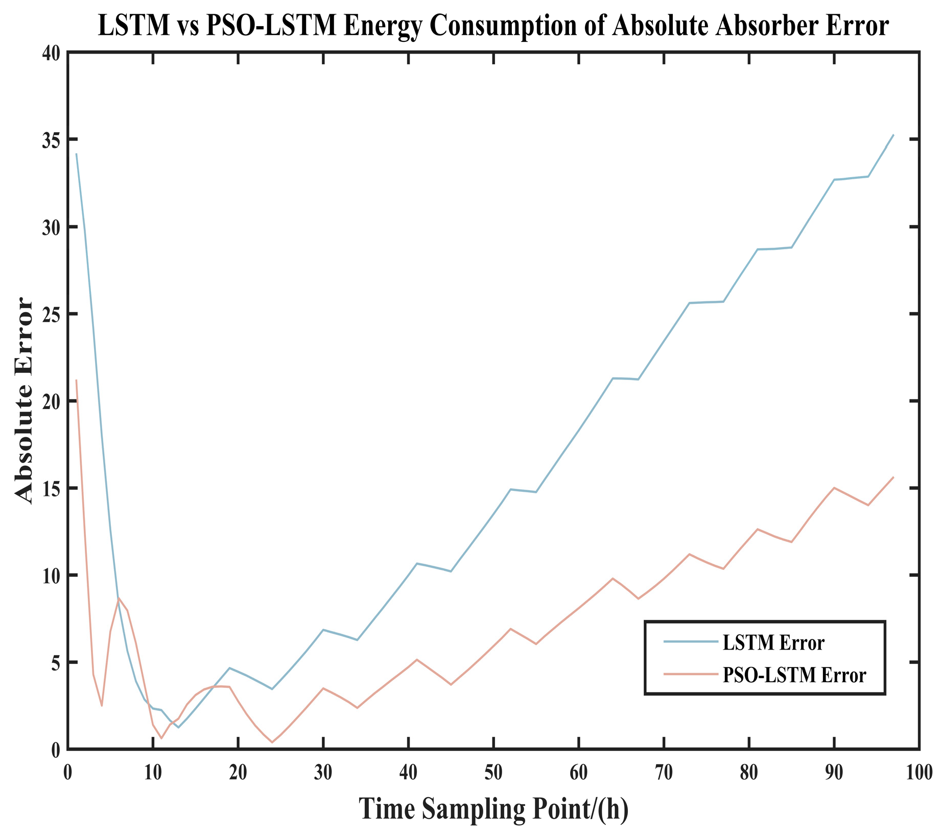
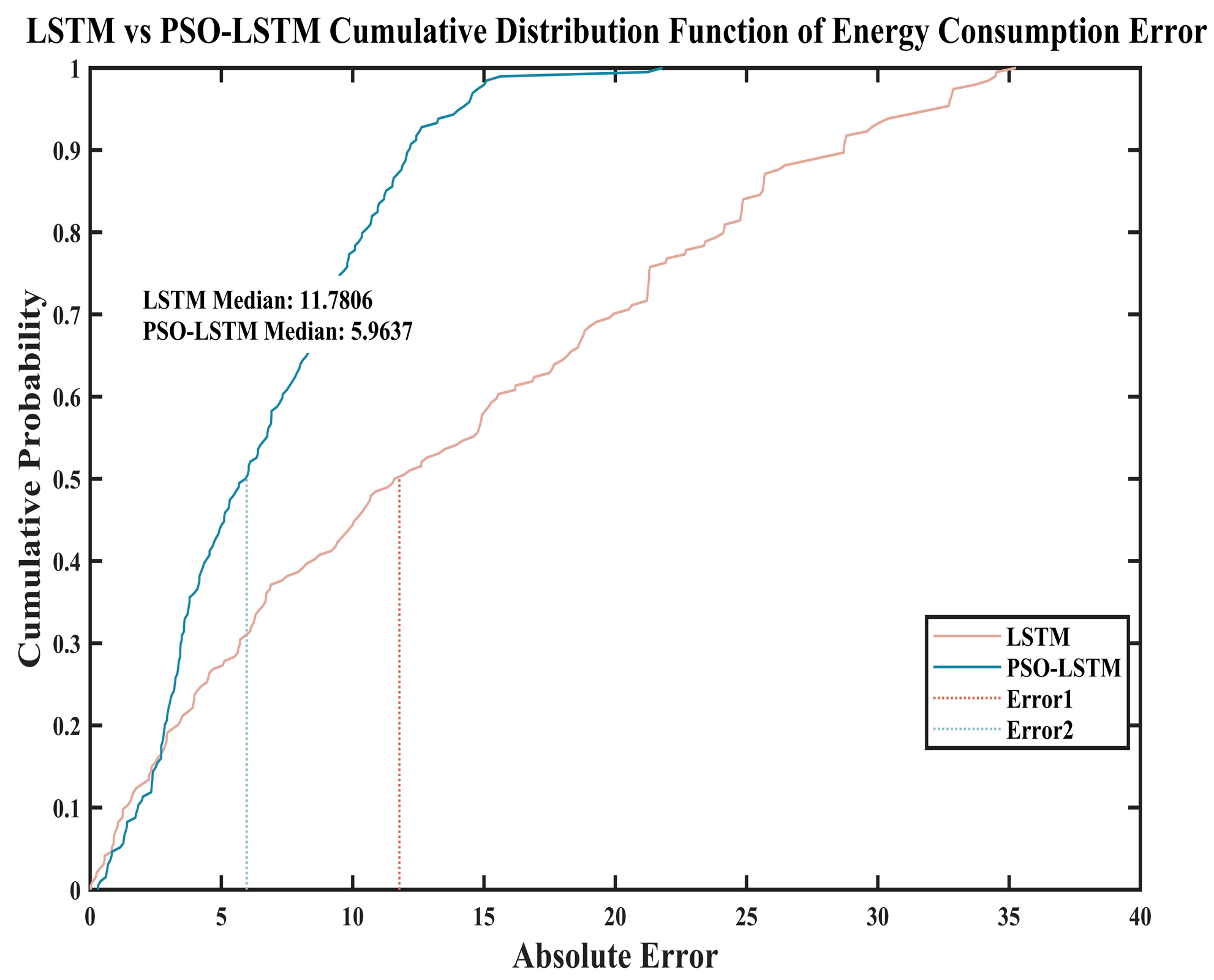
Figure 19 and Figure 20, along with

Table 18. LSTM vs. PSO-LSTM Significance Analysis Comparison of Energy Consumption.

		LSTM	PSO-LSTM	Improvement
Basic Statistical Information	Sample size	194	194
	Mean error	13.63	6.63	+51.34%
	Standard Deviation of Error	10.08	4.19	+58.45%
	Median error	11.78	5.96	+49.38%
Performance Metrics	RMSE	16.94	7.84	+53.72%
	MAE	13.63	6.63	+51.34%
	MAPE	0.92	0.45	+51.29%

RMSE: root mean squared error; MAE: mean absolute error; MAPE: average absolute percentage error.

, similarly demonstrate that after predicting energy consumption of the same 194 sample points, the PSO-LSTM model exhibits significantly superior prediction errors and model evaluation metrics compared to the LSTM model. The PSO-optimized LSTM achieves improvement rates ranging from a maximum of 58.45% to a minimum of 49.38% across all metrics. This demonstrates that the PSO algorithm significantly enhances the system energy consumption prediction capabilities of the LSTM model.

Table 19. Statistical significance test (α = 0.05).

Type	LSTM	PSO-LSTM
Test for Normality of Error	p = 0.001 **	p = 0.001 **
Wilcoxon Signed-Rank Test	p = 0 ***	Cohen’s d Effect Size = 0.91(big)

** denotes highly significant, and *** denotes extremely significant.

also indicates that the Wilcoxon Signed-Rank Test was employed because the errors did not follow a normal distribution. Furthermore, the table reveals a significant difference (p < 0.05) in the prediction of system energy consumption between the two models. The LSTM model optimized by PSO demonstrates a significant improvement in predicting system energy consumption performance.

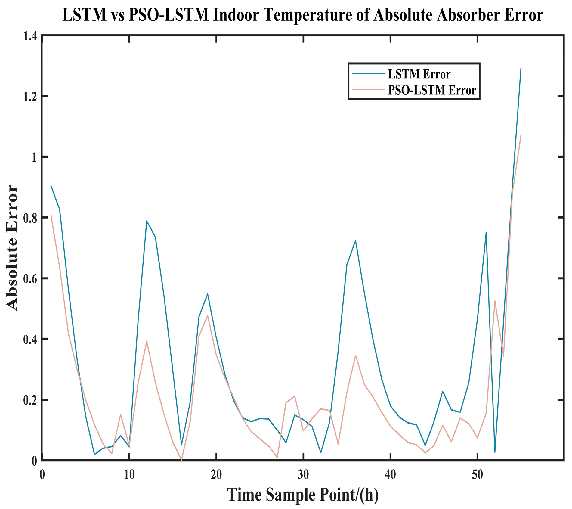
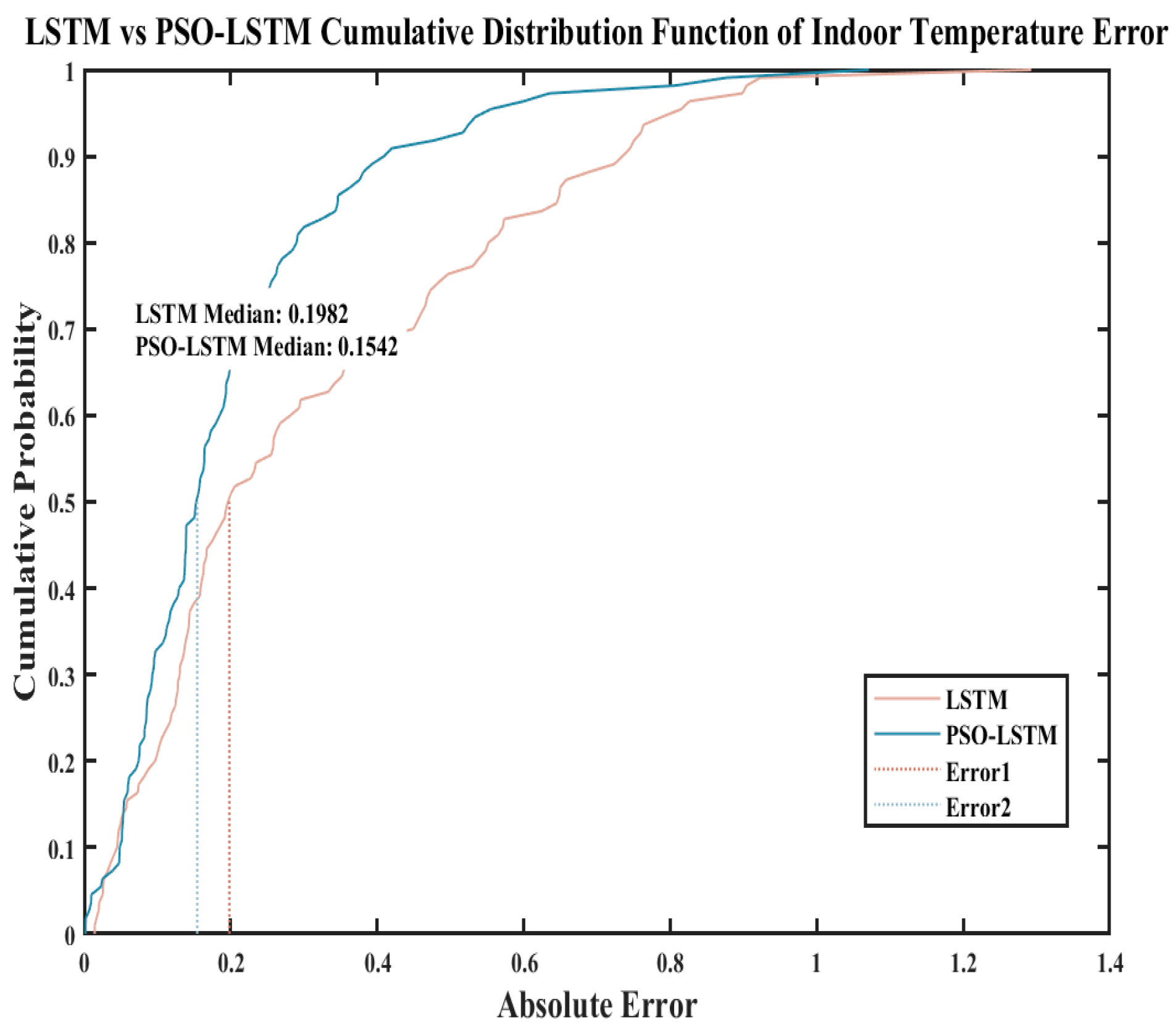
As shown in Figure 21 and Figure 22 and

Table 20. Comparative Analysis of the Significance of LSTM and PSO-LSTM in Indoor Temperature.

		LSTM	PSO-LSTM	Improvement
Basic Statistical Information	Sample size	110	110
	Mean error	0.31	0.20	+35.06%
	Standard Deviation of Error	0.27	0.18	+31.46%
	Median error	0.2	0.15	+22.16%
Performance Metrics	RMSE	0.41	0.27	+33.53%
	MAE	0.31	0.20	+35.06%
	MAPE	1.71	1.11	+34.92%

RMSE: root mean squared error; MAE: mean absolute error; MAPE: average absolute percentage error.

, after predicting indoor temperatures for the same 110 sample points, the PSO-LSTM model demonstrated significantly superior prediction errors for heat accumulation and model evaluation metrics compared to the LSTM model. The PSO-optimized LSTM achieved improvement rates of up to 35.06% for all metrics, with the minimum improvement rate at 22.16%. This demonstrates that the PSO algorithm effectively enhances the LSTM model’s performance in predicting indoor temperatures.

Table 21. Statistical significance test (α = 0.05).

Type	LSTM	PSO-LSTM
Test for Normality of Error	p = 0.0175 *	p = 0.001 **
Wilcoxon Signed-Rank Test	p = 0 ***	Cohen’s d Effect Size = 0.48 (Small)

* denotes significant, ** denotes highly significant, and *** denotes extremely significant.

indicates that the Wilcoxon Signed-rank Test was employed because the errors did not follow a normal distribution. Additionally, the table reveals a significant difference (p < 0.05) in the indoor temperature prediction capabilities between the two models, with the PSO-optimized LSTM model demonstrating improved performance. In summary, statistical significance tests conducted on both the LSTM neural network and the PSO-LSTM neural network clearly demonstrate that the PSO-LSTM neural network outperforms the LSTM neural network model.

6. Conclusions

The primary original contributions of this study are as follows:

1. A novel PSO-LSTM hybrid modeling approach is proposed to address the challenge of predicting thermal loads within the ultra-short timeframe of 7 min in heating systems, significantly enhancing the prediction accuracy of the system; 2. A simulation optimization architecture integrating TRNSYS with the intelligent PSO algorithm is constructed, achieving closed-loop verification from simulation to predictive control; 3. The research outcomes provide concrete quantitative methods for energy-saving optimization in China’s district heating systems with high renewable energy integration.

Time-series prediction models based on LSTM neural networks and PSO-LSTM neural networks were evaluated through indoor temperature, heat collection, and energy consumption simulations, using two model error metrics as outcomes.

Research indicates that under extreme snowfall conditions, the PSO-LSTM model demonstrates superior predictive performance compared to clear weather conditions. For instance, under snowfall conditions, solar radiation intensity increases by 82% and 86.7%, respectively, while the proportion of decreased solar radiation rises from 83.8% to 91.1%. By optimizing the LSTM network, the particle swarm optimization algorithm yields a set of hyperparameters with enhanced generalization capabilities. This research avoids overreliance on solar irradiance patterns, enabling deeper insights into thermodynamic patterns within the system under strong perturbations. Therefore, the PSO-LSTM model is particularly suitable for regions like southern Xinjiang with significant climate variability and occasional extreme weather events, ensuring the stability and reliability of the prediction system throughout the year. Statistical significance tests comparing the LSTM neural network and the PSO-LSTM neural network clearly demonstrate that the PSO-LSTM neural network outperforms the LSTM neural network model. In summary, the following conclusions can be drawn:

(1)

Improving the accuracy of indoor temperature prediction (R² increased by 16.5–28.3%, MAE decreased by 0.141–0.16 °C)

In residential buildings, indoor temperature reflects the ultimate thermal comfort level and the overall supply-demand relationship within the structure. Building upon this, this study proposes a novel improved method capable of accurately monitoring a building’s thermal inertia within a short timeframe. This high precision enables forward-feedback combined control. Based on predictions from the PSO-LSTM model, the method adjusts valve/pump outputs minutes to ten minutes in advance before human discomfort occurs. This shifts control from “passive regulation” to “proactive regulation,” completely eliminating indoor temperature overshooting and undercooling, significantly enhancing comfort. Compared to the literature (Yang et al., 2025 [26]), the R² value approaches 1, demonstrating superior predictive accuracy and comfort performance of this research model.

(2)

Significantly Enhanced Solar Energy Collection Prediction Accuracy (R² improved by 82–86.7%, RMSE reduced by 70–80%)

Solar energy collection represents the instantaneous contribution of free energy—solar power. This approach substantially enhances the predictive capability for “renewable energy resources.” Building upon this foundation, high-precision solar energy collection predictions enable optimized configuration of energy management systems. For instance, when a significant increase in heat collection is forecasted within the next 10 min, natural gas boilers and air-source heat pumps can be reduced in advance to prioritize solar energy utilization. Conversely, auxiliary heat sources can be activated early to suppress peak loads. This directly correlates with the reduced system energy consumption observed in the study. Compared to the literature (Cao et al., 2024 [19]), the R² value is closer to 1, demonstrating the higher predictive accuracy of the research model.

(3)

Enhanced system energy consumption prediction accuracy (MAPE reduced by nearly 80%)

System energy consumption comprehensively reflects the operational status of various equipment. High-precision forecasting forms the foundation for achieving full-system digital and intelligent control. It is crucial for managing interactions within the power system and controlling costs. In regions implementing time-of-use electricity pricing policies, operators can leverage precise energy consumption forecasts to maximize heat storage during off-peak periods. During high-price periods, they can rely on energy storage and solar power generation to minimize operational costs. This research provides essential theoretical foundations and technical support for power system applications.

In summary, this work lays the groundwork for establishing a closed-loop intelligent control chain encompassing “sensing-prediction-decision-optimization.” By precisely capturing critical operational parameters, it transitions from time-delay control based on current conditions to forward-looking optimization grounded in future operational scenarios. Research indicates that the predictive control method centered on the PSO-LSTM model holds broad application prospects in southern Xinjiang, with the potential to further reduce building energy consumption by 10–15%, demonstrating significant engineering application potential.