Analysis of Demand Response in Electric Systems with Strong Presence of Intermittent Generation Using Conditional Value-at-Risk

Abstract

The integration of renewable sources, such as hydro, wind, and solar power, into electrical systems has profoundly transformed the sector’s dynamics. The inherent intermittency of these energy sources, due to the uncertainty associated with inflows, winds, and solar irradiation, introduces considerable challenges in the operation and planning of the electrical system. In this context, demand response emerges as a promising solution to handle the fluctuations in renewable generation and maintain system stability and reliability. Therefore, this study presents a new approach to the demand response program through the modeling of an optimal power flow problem to minimize operational costs, considering the uncertainties in hydro, wind, and solar generation by applying the Conditional Value-at-Risk (CVaR) risk metric. The mathematical modeling of the problem was conducted, and the problem was solved using the MINOS solver. To validate the model, simulations were carried out using modified IEEE systems of 14, 30, 57, and 118 buses, considering operation planning for the next 24 h. Furthermore, sensitivity analyses were performed by altering the CVaR parameters. As a result of the simulations, the total operational cost, electrical losses, and hourly generation at each bus by source type were determined, highlighting how CVaR impacts the operation of this type of system.

1. Introduction

Demand response (DR) mechanisms in electrical systems have been increasingly growing worldwide in recent years. The operational flexibility provided by these mechanisms becomes progressively more important as grids become more congested and increasingly dominated by intermittent generation sources such as wind and solar [1]. The International Energy Agency (IEA) noted that the presence of DR in electrical systems is expected to continue accelerating until 2050, with the availability of DR worldwide anticipated to increase tenfold from 2020 to 2030 [2].

The integration of intermittent renewable energy sources, such as solar and wind, imposes significant challenges on the operation of electrical systems due to their variable and unpredictable nature [3]. To address these challenges, demand response (DR) emerges as a strategic solution, offering the necessary flexibility to balance supply and demand in real-time. However, the increasing intermittency and variability of renewable generation demand more sophisticated approaches for managing power flow in electrical systems subject to these uncertainties [4].

The optimal power flow problem given the uncertainty of intermittent generation is a significant challenge in the operation of electrical systems that utilize renewable energy sources, such as wind, solar, and, to a lesser extent, hydro power. The uncertainty associated with intermittent renewable energy generation can lead to inefficient operation of the electrical system, with negative impacts on the quality of supplied power, system security, and operating costs. To address the stochasticity in the optimal power flow problem, various approaches exist, including stochastic programming, Monte Carlo simulation, machine learning, and the use of risk metrics [5,6].

In stochastic programming, the problem is formulated as a mathematical program that takes into account the uncertainty in intermittent renewable energy generation, using techniques such as Markov chains to model the dynamics of uncertainty scenarios. In Monte Carlo simulation, multiple scenarios of intermittent renewable energy generation are generated from historical data or statistical models, allowing the evaluation of system performance and obtaining the optimal solution. Machine learning, a subfield of artificial intelligence, deals with computational algorithms that can be improved through training data without explicit programming, presenting itself as a fundamental tool for modeling the uncertainty associated with intermittent generation. This allows quantifying the probability of different generation scenarios and adjusting model parameters after training [7]. Finally, the Conditional Value-at-Risk (CVaR) risk method, widely used in economics, indicates the average size of potential losses in a generation or storage system over a specific period, considering adverse scenarios, thus offering a comprehensive measure of risk by including the average excess loss [7,8].

The choice of CVaR for handling uncertainties in renewable generation in the day-ahead operation planning problem was motivated by its ability to provide a robust and conservative assessment of the risks associated with these uncertainties. Although methods such as Markov chains and machine learning have been explored in other studies, CVaR stands out for its direct applicability in contexts where minimizing extreme losses and capturing the tail behavior of probability distributions are crucial. Unlike a Markov chain, which models state transitions based on conditional probabilities, and machine learning approaches, which often require large volumes of historical data and can introduce additional complexity into the modeling, CVaR offers a more transparent and interpretable solution for incorporating risk into power flow optimization. This characteristic makes it particularly suitable for operation planning problems, where mitigating adverse scenarios is a priority, enabling more effective management of the uncertainties inherent in renewable generation.

1.1. Utilization of Demand Response in Operation Planning

The integration of DR into operation planning has become increasingly crucial in optimizing energy management and enhancing the flexibility and reliability of power systems.

Duan [3] addressed the challenges of demand-side power consumption variation by proposing a day-ahead scheduling model that incorporates price-based demand bidding, allowing for price-elastic demand responses. Using simulations on the IEEE 30-bus system, the study demonstrated that integrating price-elastic demand bids can effectively balance demand fluctuations, enhance social welfare, and increase the surplus for load-serving entities. Jiang et al. [9] developed an optimal real-time pricing model based on demand response, designed to encourage customer participation in electricity market operations. The model was validated using the IEEE 24-bus system, further demonstrating the effectiveness of DR in modern power grids. Heydarian-Forushani et al. [10] further expanded on this by presenting a novel linear framework for optimizing DR programs, focusing on determining the optimal location, type, and penetration rate of DR initiatives within the network-constrained unit commitment. Their methodology, tested on the IEEE 24-bus system, emphasized the importance of selecting appropriate DR strategies based on customer price elasticity to maximize the benefits of DR programs. Sun et al. [11] proposed a day-ahead optimal scheduling strategy for integrated electricity and thermal systems, incorporating multiple types of demand response. Their study highlights the use of situation awareness technology to address uncertainties in renewable energy sources, demonstrating how diverse DR mechanisms can improve system energy efficiency and promote renewable energy consumption.

1.2. Handling Uncertainties in the Power Flow Problem

The handling of uncertainties in power flow, particularly in the context of renewable energy integration and load variability, has become increasingly important in ensuring the reliable and efficient operation of power systems.

In a study by Luo and Zhang [12], a two-stage dispatch model for a Virtual Power Plant (VPP) was developed to manage uncertainties in wind, solar power, and load. By using demand response strategies, the model optimizes load profiles and reduces costs, enhancing the economic stability of the VPP. Lu et al. [13] proposed a robust stochastic stability analysis approach considering wind speed prediction errors in power systems. Using Markov modeling and linear matrix inequality techniques, they developed a method to analyze the stochastic stability of wind power systems under varying transition probability assumptions, demonstrating high computational efficiency without needing to track the actual system trajectory. Arun et al. [14] proposed a priority-based load-shifting demand response strategy to reduce peak demand and balance supply and demand in the presence of increased renewables, focusing on residential markets. Kang and Lee [15] introduced a data-driven prediction method for load curtailment in demand response systems, addressing the uncertainty of customer participation by using a weighted ensemble model to predict energy reductions more accurately based on electricity consumption data and past demand response events. Miraftabzadeh et al. [16] reviewed the potential of machine learning techniques in power grids, emphasizing their advantages over traditional methods, particularly in providing accurate short-term power flow forecasts with greater computational efficiency, scalability, and potential applications in smart grids. Khaloie et al. [17] provided an overview of machine learning applications in solving the optimal power flow problem, highlighting how recent advances in machine learning can help grid operators address the computational challenges of real-time optimal power flow solutions, thereby enhancing the efficiency and reliability of power system operations.

1.3. Application of CVaR in the Power Flow Problem

The application of CVaR can be found in several studies in the literature. Firouz et al. [18] evaluated the uncertainty of wind generators in the electricity market considering demand response and risk aversion to achieve profits in their participation in the energy market. Gong and Wang [19] proposed a coordinated dispatch optimization model considering demand response and energy storage with the CVaR metric incorporated to meet risk criteria. Jabr [20] considered a distributionally robust framework to solve the optimal power flow problem in the presence of intermittent renewable generation. More recently, Singh et al. [17] analyzed the economic risk of an integrated wind and reversible hydroelectric generation system where the CVaR risk metric was considered as a risk assessment tool for a modified IEEE 30-bus system over a 24 h horizon.

1.4. Objectives and Contributions of This Work

In this work, a modeling of electrical systems with a strong presence of renewable sources and demand response is carried out to evaluate the day-ahead operation scheduling. Unlike other works, here CVaR is used in handling the information on the availability of hydraulic, wind, and solar resources available for the day-ahead operation, aiming to increase operational security.

The simulations were conducted considering the IEEE systems of 14, 30, 57, and 118 buses with the objective of evaluating the total operational cost and electrical losses by varying the system’s demand response potential and the CVaR parameters.

The main contributions of this work are as follows:

• Contextualization of the problem from the perspective of various authors and evaluation of how CVaR has been used in this type of problem;
• Proposal of a new use of CVaR, where it is applied to the expected renewable resources in the input of the day-ahead operation problem;
• Modeling, simulation, and analysis of various scenarios to evaluate the proposed model.

The article is organized as follows: the modeling of the electrical system with demand response and generation uncertainties using the CVaR metric is presented in Section 2. Section 3 presents the simulation results for the IEEE systems of 14, 30, 57, and 118 buses. Finally, the conclusions are presented in Section 4.

2. Modeling of Demand Response and Generation Uncertainties with the CVaR Metric

This section details the modeling of the day-ahead operation planning problem of the electrical system in the presence of demand response and a significant integration of renewable generation. In this model, the electrical system is modeled as a linearized power flow problem, given that the focus of this work is on system operation planning, where CVaR is applied to the input data of renewable resource availability.

2.1. Demand Response in Electrical System Operation

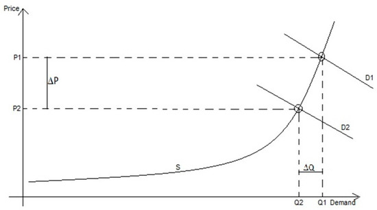
The electricity produced by generators is dispatched in merit order, starting with the generators with the lowest marginal cost until meeting the instantaneous demand for electricity. In most power systems, the spot price of electricity represents the marginal cost of the highest-cost generator that is injecting power. Figure 1 illustrates the effect of DR on the elasticity of electricity demand. The inelastic demand in the electricity market is represented by curve D1. The supply curve S is based on marginal cost, with the lower-cost generation producing first. The high price P1 associated with the inelastic demand D1 is extrapolated from the intersection point of the supply curve S and the demand curve D1. When DR measures are introduced, the demand becomes more elastic, represented by curve D2. The new equilibrium point given by the same supply curve S and the more elastic demand curve D2 provides a lower price [21].

Figure 1. Effects of DR on the price (P) and demand (Q) of electricity (Adapted from [21]).

2.2. Objective Function of the Problem

Considering that the approach proposed in this work is based on the modeling of an optimal power flow problem, the objective function is the one that must be optimized concerning the control variables, within the limits imposed by the constraints. The objective function of this work is the minimization of the operational cost of the electrical system, represented by Equation (1), which includes the costs of thermal generation, hydro generation, and demand response for the 24 h operational planning of the system, detailed in Equations (2)–(4), respectively. Solar and wind generation are not defined in the objective function because they are considered non-dispatchable, meaning there will always be generation as long as solar irradiation or wind is available.

$$min {\displaystyle \sum }_{t=1}^{24}{\displaystyle \sum }_{i=1}^{NB}\left(C{T}_{i,t}+C{H}_{i,t}+CD{R}_{i,t}\right)$$

(1)

$${CT}_{i,t}=a_i·{PT}_{i,t}^2+b_i·{PT}_{i,t}+c_i$$

(2)

$${CDR}_{i,t}={DR}_{i,t}·{CostDR}_{i,t}$$

(3)

$${CH}_{i,t}={PH}_{i,t}·{CostH}_{i,t}$$

(4)

where $i$ is a bus of the system; $NB$ is the number of buses in the system; $t$ represents the hour; ${CT}_{i,t}$ is the cost of thermal generation at bus $i$ at hour $t$ (R$); ${PT}_{i,t}$ is the thermal generation at bus $i$ at time $t$ (W); $a_i$, $b_i$, and $c_i$ are the thermal generation constants at bus $i$ (R$/W², R$/W, R$, respectively); ${CH}_{i,t}$ is the cost of hydro generation at bus $i$ at hour $t$ (R$); ${PH}_{i,t}$ is the hydro generation at bus $i$ at hour $t$ (W); ${CostH}_{i,t}$ is the unit cost of hydro generation at bus $i$ at hour $t$ (R$/MWh); ${CDR}_{i,t}$ is the cost of demand response at bus $i$ at hour $t$ (R$); ${DR}_{i,t}$ is the reduction in DR at bus $i$ at hour $t$ (W); and ${CostDR}_{i,t}$ is the unit cost of DR at bus $i$ at hour $t$ (R$/MWh).

Hydro generation, in turn, is modeled in cascade, and the hydroelectric production function that relates the power output of the hydroelectric plant with the reservoir level, inflow, and spill is provided by Equation (5), which describes the relationship between the released water and the reservoir head with the power generated by the plant. The coefficients $c_1^h$, $c_2^h$, $c_3^h$, $c_4^h$, $c_5^h$, and $c_6^h$ are the characteristic factors of the hydro plant h and are related to the type of turbine and reservoir [22,23].

$${PH}_{i,t}=c_{1,i}·{L_{i,t}}^2+c_{2,i}·{\left(R_{i,t}+I_{i,t}\right)}^2+c_{3,i}·\left(R_{i,t}+I_{i,t}\right)\ast L_{i,t}+c_{4,i}·L_{i,t}+c_{5,i}·\left(R_{i,t}+I_{i,t}\right)+c_{6,i}$$

(5)

where $c_{1\to 6,i}$ are the hydro generation constants at bus $i$ (W.s²/m⁶, W.s²/m⁶, W.s²/m⁶, W.s/m³, W.s/m³, and W, respectively); $L_{i,t}$ is the reservoir volume at bus $i$ at hour $t$ (m³/s); $R_{i,t}$ is the water discharged from the reservoir at bus $i$ at hour $t$ (m³/s); and $I_{i,t}$ is the inflow into the reservoir at bus $i$ at hour $t$ (m³/s).

The costs of wind and solar generation are not included in the objective function because, for the purposes of electrical system operation, these sources are non-dispatchable. However, the impacts of these sources on the objective function values are relevant, as their generation directly affects the amount of thermal generation, hydro generation, and demand response resources dispatched for a given hour of operation, as shown in the equality constraints.

2.3. Equality Constraints

Equality constraints are those that require a linear combination of the decision variables to be equal to a constant value. In the proposed model, these constraints at buses $i$ correspond to the active power balance equation and the power from wind and solar generation. For the lines $ik$, the equality constraint is the power flow on the line.

Equation (6) establishes the active power balance relationships of the system. Equations (7)–(9) describe the total, wind, and solar generation at each bus, respectively. The impact of demand response on the load at a given bus is represented by Equation (10). Equations (11) and (12) pertain to the considerations regarding the linearized power flow in the electrical system.

$${Pi}_{i,t}={Pg}_{i,t}-{Pload}_{i,t}^{RD}-{Plosses}_{i,t}=\sum _{kϵ{\mathsf{\Omega }}_{\mathrm{i}}}{b^{\prime }}_{ik} ·{ \theta }_{ik,t}$$

(6)

$${Pg}_{i,t}={PT}_{i,t}+{PH}_{i,t}+{PW}_{i,t}+{PS}_{i,t}$$

(7)

$${PW}_{i,t}=\left\{\begin{array}{c}0, v_{i,t}\le v_{cutin,i}\\ a_{1,i}{v_{i,t}}^3+b_{1,i}{v_{i,t}}^2+c_{1,h}{v}_{i,t}+d_{1,i}, v_{cutin,i}<v_{i,t}<v_{1,i} \\ a_{2,i}{v_{i,t}}^3+b_{2,i}{v_{i,t}}^2+c_{2,i}{v}_{i,t}+d_{2,i}, v_{1,i}\le v_{i,t}<v_{2,i} \\ {Pn}_i, v_{2,i}\le v_{i,t}<v_{cutout,i}\\ 0, v_{i,t}\ge v_{cutout,i}\end{array}\right.$$

(8)

$$P{S}_{i,t}=A_i·{\mathsf{\eta }}_{\mathrm{i}}·P{R}_i·G_{i,t}$$

(9)

$$Ploa{d}_{i,t}^{DR}=Ploa{d}_{i,t}-D{R}_{i,t}$$

(10)

$$V_{i,t}=1$$

(11)

$$P_{ik,t}={\displaystyle \frac{{\theta }_{i,t}-{\theta }_{k,t}}{x_{ik}}}+{\displaystyle \frac{{\phi }_{i,t}-{\phi }_{k,t}}{x_{ik}}}$$

(12)

where ${\mathsf{\Omega }}_i$ is the set of neighboring buses of bus $i$; $k$ is a neighboring bus of bus $i$; $ik$ is the line between buses $i$ and $k$; $P{i}_{i,t}$ is the active power injection at bus $i$ at hour $t$ (W); $P{g}_{i,t}$ is the active power generation at bus $i$ at hour $t$ (W); $P{W}_{i,t}$ is the wind generation at bus $i$ at hour $t$ (W); $P{n}_i$ is the nominal power of the wind turbine at bus $i$ (W); $v_i$ is the wind speed at the axis of the wind turbine at bus $i$ (m/s); $v_{cutin,i}$ is the cut-in wind speed of the wind turbine at bus $i$ (m/s); $v_{cutout,i}$ is the cut-out wind speed of the wind turbine at bus $i$ (m/s); $v_{1,i}$ is the inflection point wind speed of the generation curve at bus $i$ (m/s); $v_{2,i}$ is the start speed of the nominal speed zone at bus $i$ (m/s); $a_{1,i}, b_{1,i}, c_{1,i} \mathrm{and} d_{1,i}$ are the coefficients of the polynomial describing the generation curve between the cut-in and inflection speeds at bus $i$ (W.s³/m³, W.s²/m², W.s/m, and W, respectively); $a_{2,i}, b_{2,i}, c_{2,i} \mathrm{and} d_{2,i}$ are the coefficients of the polynomial describing the generation curve between the inflection speed and the start of the nominal zone at bus $i$ (W.s³/m³, W.s²/m², W.s/m, and W, respectively); $P{S}_{i,t}$ is the solar generation at bus $i$ at hour $t$ (W); $A_i$ is the area covered by the photovoltaic generation at bus $i$ (m²); ${\mathsf{\eta }}_i$ is the efficiency of the photovoltaic panels at bus $i$ (%); $P{R}_i$ is the efficiency of the photovoltaic system at bus $i$ (%); $G_{i,t}$ is the solar irradiation incident on the modules at bus $i$ at hour $t$ (W/m²); $Ploa{d}_{i,t}^{DR}$ is the active load at bus $i$ at hour $t$ after the DR program activation (W); $Ploa{d}_{i,t}$ is the active load at bus $i$ at hour $t$ before the DR program activation (W); $Plosse{s}_{i,t}$ is the active electrical loss allocated to bus $i$ at hour $t$ (W); ${b^{\prime }}_{ik}$ is the nodal admittance value at position $ik$ of the $B^{\prime }$ matrix (S); ${\theta }_{ik,t}$ is the phase angle difference between buses $i$ and $k$ at hour $t$ (rad); ${\theta }_{i,t}$ is the phase angle at bus $i$ at hour $t$ (rad); ${\theta }_{k,t}$ is the phase angle at bus $k$ at hour $t$ (rad); ${\phi }_{i,t}$ is the transformer phase shift at bus $i$ at hour $t$ (rad); ${\phi }_{k,t}$ is the transformer phase shift at bus $k$ at hour $t$ (rad);$V_{i,t}$ is the voltage at bus $i$ at hour $t$ (pu); and $P_{ik,t}$ is the power flow on the line between buses $i$ and $k$ at hour $t$ (W).

2.4. Inequality Constraints

Inequality constraints in the optimal power flow problem describe upper or lower limits for certain variables that must be respected to ensure the safety and reliability of the electrical system. These constraints include the limits on energy consumption and generation at the network buses, the individualized generation limits of each asset separated by the generation source, participation limits in demand response, and active power flow limits on transmission lines.

The active power generation limits are related to the maximum generation capacity of each source at each hour and are represented by Equations (13)–(17). The minimum limits represent the inflexibility of generation for thermal generation and the minimum safe flow regime for hydro generation. In the case of wind and solar generation, the minimum limits are zero, representing moments when there is no available renewable resource for generation. Regarding the system load and demand response, Equations (18) and (19) represent the inequality constraints that must be satisfied, respectively. The power flow limits at line ik are represented by Equation (20).

$$Pgmi{n}_{i,t}\le P{g}_{i,t}\le Pgma{x}_{i,t}$$

(13)

$$PTmi{n}_{i,t}\le P{T}_{i,t}\le PTma{x}_{i,t}$$

(14)

$$PHmi{n}_{i,t}\le P{H}_{i,t}\le PHma{x}_{i,t}$$

(15)

$$PWmi{n}_{i,t}\le P{W}_{i,t}\le PWma{x}_{i,t}$$

(16)

$$PSmi{n}_{i,t}\le P{S}_{i,t}\le PSma{x}_{i,t}$$

(17)

$$Ploadmi{n}_{i,t}\le Ploa{d}_{i,t}\le Ploadma{x}_{i,t}$$

(18)

$$DRmi{n}_{i,t}\le D{R}_{i,t}\le DRma{x}_{i,t}$$

(19)

$$Pmi{n}_{ik,t} \le P_{ik,t} \le Pma{x}_{ik,t}$$

(20)

where $Pgmi{n}_{i,t}$ and $Pgma{x}_{i,t}$ are the minimum and maximum active power generations, respectively, at bus $i$ at hour $t$ (W); $PTmi{n}_{i,t}$ and $PTma{x}_{i,t}$ are the minimum and maximum thermal generations, respectively, at bus $i$ at hour $t$ (W); $PHmi{n}_{i,t}$ and $PHma{x}_{i,t}$ are the minimum and maximum hydro generations, respectively, at bus $i$ at hour $t$ (W); $PWmi{n}_{i,t}$ and $PWma{x}_{i,t}$ are the minimum and maximum wind generations, respectively, at bus $i$ at hour $t$ (W); $PSmi{n}_{i,t}$ and $PSma{x}_{i,t}$ are the minimum and maximum solar generations, respectively, at bus $i$ at hour $t$ (W); $Ploadmi{n}_{i,t}$ and $Ploadma{x}_{i,t}$ are the minimum and maximum active loads, respectively, at bus $i$ an hour $t$ before DR (W); $DRmi{n}_{i,t}$ and $DRma{x}_{i,t}$ are the minimum and maximum load reductions, respectively, at bus $i$ at hour $t$ (W); and $Pmi{n}_{ik,t}$ and $Pma{x}_{ik,t}$ are the minimum and maximum power flows, respectively, on the line between buses $i$ and $k$ at hour $t$ (W).

2.5. Loss Allocation

To consider the active losses distributed across all buses of the electrical system, the problem must be solved in two stages. In the first stage, electrical losses are considered null according to Equation (21), and Equation (1) is solved to obtain a vector ${\theta }_{ik,t}^{\prime }$ according to Equation (6). The approximate losses are then calculated from ${\theta }_{ik,t}^{\prime }$ and distributed as additional loads through the vector $Plosse{s}_{i,t}$ according to Equation (22). The problem is then solved again with the losses to determine the new value for the objective function and the phase angles ${\theta }_{ik,t}$ [24].

$$Plosse{s}_{ik,t}^{\prime }=0\to {\theta }_{ik,t}^{\prime }$$

(21)

$$Plosse{s}_{i,t}={\displaystyle \frac{1}{2}}{\displaystyle \sum }_{kϵ{\mathsf{\Omega }}_i}{g}_{ik}{\theta }_{ik,t}^{\prime }$$

(22)

where $Plosse{s}_{ik,t}^{\prime }$ is the loss considered in the first stage of the solution; ${\theta }_{ik,t}^{\prime }$ is the phase angle difference between buses $i$ and $k$ at hour $t$ in the first stage of the solution (rad); and $g_{ik}$ is the nodal conductance value at position $ik$ of the $G$ matrix (S).

2.6. Managing Renewable Generation Uncertainty Using CVaR

The CVaR risk metric was first introduced by Artzner et al. [25]. CVaR is measured based on the average of the worst expected losses over a given time interval and a certain confidence level. In the case of the electric sector, this criterion is applied, for example, by assigning a higher weight to the worst-case scenarios to enhance the security of system operation. Mathematically, the CVaR (ϕ_β) of a distribution of expected returns can be formulated according to Equations (23) and (24) [26,27].

$${\varnothing }_{\beta }=E[z|z\ge {\alpha }_{\beta }\left(x\right)]$$

(23)

$${\varnothing }_{\beta }={{\displaystyle \int }}_{-\infty }^{+\infty }z.p\left(w|z\ge {\alpha }_{\beta }\left(x\right)\right)dw$$

(24)

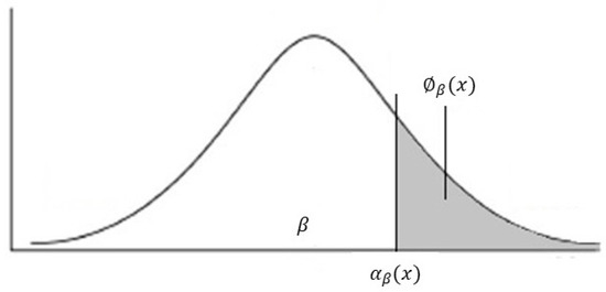
In Equation (23), the variable ${\varnothing }_{\beta }$ represents the expected value or conditional expectation of a variable $z$, given that $z$ is greater than or equal to a certain threshold ${\alpha }_{\beta }\left(x\right)$. The term is a notation that represents the conditional expectation of the variable $z$, given that $z$ is greater than or equal to ${\alpha }_{\beta }\left(x\right)$. The conditional expectation is the average value that $z$ assumes, given that the condition $z$ $\ge$ ${\alpha }_{\beta }\left(x\right)$ is satisfied. From a probabilistic point of view, this means that ${\varnothing }_{\beta }$ is the expected average value of the variable $z$, considering only the cases where $z$ reaches or exceeds the threshold ${\alpha }_{\beta }\left(x\right)$. In Equation (24), $p\left(w|z\ge {\alpha }_{\beta }\left(x\right)\right)$ represents the conditional density function of a variable $w$, given that $z$ is greater than or equal to ${\alpha }_{\beta }\left(x\right)$. In other words, this tells us the probability of $w$ given that the condition $z$ $\ge$ ${\alpha }_{\beta }\left(x\right)$ is satisfied, and the integration over $w$ from $-\infty$ to $+\infty$ indicates that all possible realizations of $w$ are considered. In Figure 2, Equation (24) is represented graphically.

Figure 2. Loss frequency distribution and CVaR (Adapted from [28]).

For the proposed model, the inputs are the expected wind, rainfall, and irradiation curves for the day-ahead operation, which will directly impact the operation due to the strong presence of renewable sources in the system. The definitions of the renewable resource are made by applying the CVaR methodology, defining the parameters α and λ of this metric based on the hourly historical series of the renewable resource for that specific day of operation, ordered from smallest to largest. Equations (25)–(34) represent the mechanism used to calculate the renewable resource curves under the CVaR metric.

$$I_{i,t}=\left(1-\lambda \right)·I_{{avg}_i}+\lambda ·CVa{R}_{I,\alpha ,i,t}$$

(25)

$$v_{i,t}=\left(1-\lambda \right)·v_{{avg}_i}+\lambda ·CVa{R}_{v,\alpha ,i,t}$$

(26)

$$G_{i,t}=\left(1-\lambda \right)·G_{{avg}_i}+\lambda ·CVa{R}_{G,\alpha ,i,t}$$

(27)

$$CVa{R}_{I,\alpha ,i,t}={\displaystyle \frac{1}{{\alpha }_{\beta }}}{\displaystyle \sum }_{n=1}^{{\alpha }_{\beta }}{I}_{n,i,t}$$

(28)

$$CVa{R}_{v,\alpha ,i,t}={\displaystyle \frac{1}{{\alpha }_{\beta }}}{\displaystyle \sum }_{n=1}^{{\alpha }_{\beta }}{v}_{n,i,t}$$

(29)

$$CVa{R}_{G,\alpha ,i,t}={\displaystyle \frac{1}{{\alpha }_{\beta }}}{\displaystyle \sum }_{n=1}^{{\alpha }_{\beta }}{G}_{n,i,t}$$

(30)

$$I_{av{g}_{i,t}}= {\displaystyle \frac{1}{N_T}}{\displaystyle \sum }_{n=1}^I{I}_{n,i,t}$$

(31)

$$v_{av{g}_{i,t}}= {\displaystyle \frac{1}{N_T}}{\displaystyle \sum }_{n=1}^v{v}_{n,i,t}$$

(32)

$$G_{av{g}_{i,t}}= {\displaystyle \frac{1}{N_T}}{\displaystyle \sum }_{n=1}^G{G}_{n,i,t}$$

(33)

$${\alpha }_{\beta }=INT \left(N_T·\alpha \right)$$

(34)

where $I$ is the set of rainfall series (mm); $v$ is the set of wind series (m/s); $G$ is the set of irradiation series (W/m²); $n$ is the historical series of the respective source; $N_T$ is the total number of historical series; $\alpha$ is the percentage of the worst scenarios to be considered; $\lambda$ is the weight of the α% worst scenarios; $CVa{R}_{I,\alpha ,i,t}$ is the Conditional Value-at-Risk of the α% worst scenarios of the water resource at bus $i$ at hour $t$ (mm); $CVa{R}_{v,\alpha ,i,t}$ is the Conditional Value-at-Risk of the α% worst scenarios of the wind resource at bus $i$ at hour $t$ (m/s); $CVa{R}_{G,\alpha ,i,t}$ is the Conditional Value-at-Risk of the α% worst scenarios of the solar resource at bus $i$ at hour $t$ (W/m); and ${\alpha }_{\beta }$ is the Value-at-Risk.

2.7. Implemented Algorithm

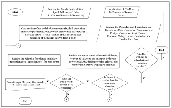
Figure 3 illustrates the flowchart of the proposed routine for this work. In this sense, the flowchart presents the mechanism of the proposed algorithm, starting with the application of the CVaR metric to the renewable resource data, reading the system parameters, and solving the problem.

Figure 3. Algorithm used for problem solution.

2.8. Computational Implementation

The computational implementation of this work was carried out using the A Mathematical Programming Language (AMPL) programming environment. In this context, Bedrinana et al. [29] tested various solvers for solving the optimal power flow problem to determine which ones require fewer iterations and less time to solve the problem. The solvers IPOPT, KNITRO, LOQO, MINOS, and SNOPT were tested on the standard 14-bus and 57-bus systems, and the conclusion of the study was that the best performances were obtained with KNITRO and MINOS, both showing similar performances, as these two solvers presented the fewest iterations and the shortest computational time to solve the problem.

In this work, the Modular In-core Nonlinear Optimization System (MINOS) solver was used. This solver uses the primal–dual simplex method to solve linear programming problems and the Newton method to solve nonlinear programming problems. It is capable of solving optimization problems involving hundreds of thousands of variables and constraints and is especially useful for solving linear optimization problems with very sparse linear constraints, meaning problems in which most of the constraints are zero [30,31].

2.9. Analyzed Electrical Systems

The 14-, 30-, 57-, and 118-bus electrical systems considered in this study are widely used test models adapted from the Institute of Electrical and Electronics Engineers (IEEE) benchmark networks. These systems represent simplified configurations of electric power transmission networks, where each bus corresponds to a point of interconnection, such as substations, generators, or loads. The 14-bus system, for example, is a basic model used in this work for initial validation of methods, while the 30-, 57-, and 118-bus systems represent more complex networks and are used to test the scalability and effectiveness of the proposed approaches. The choice of these systems allows for a robust comparative analysis, as they offer varied and challenging scenarios to evaluate the performance of the applied methodologies, such as the integration of renewable sources and the application of CVaR in power flow optimization.

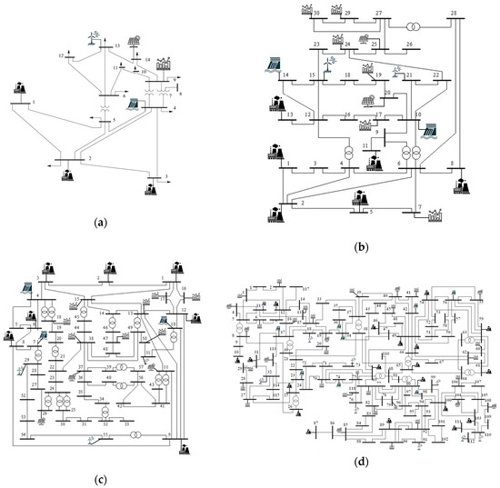
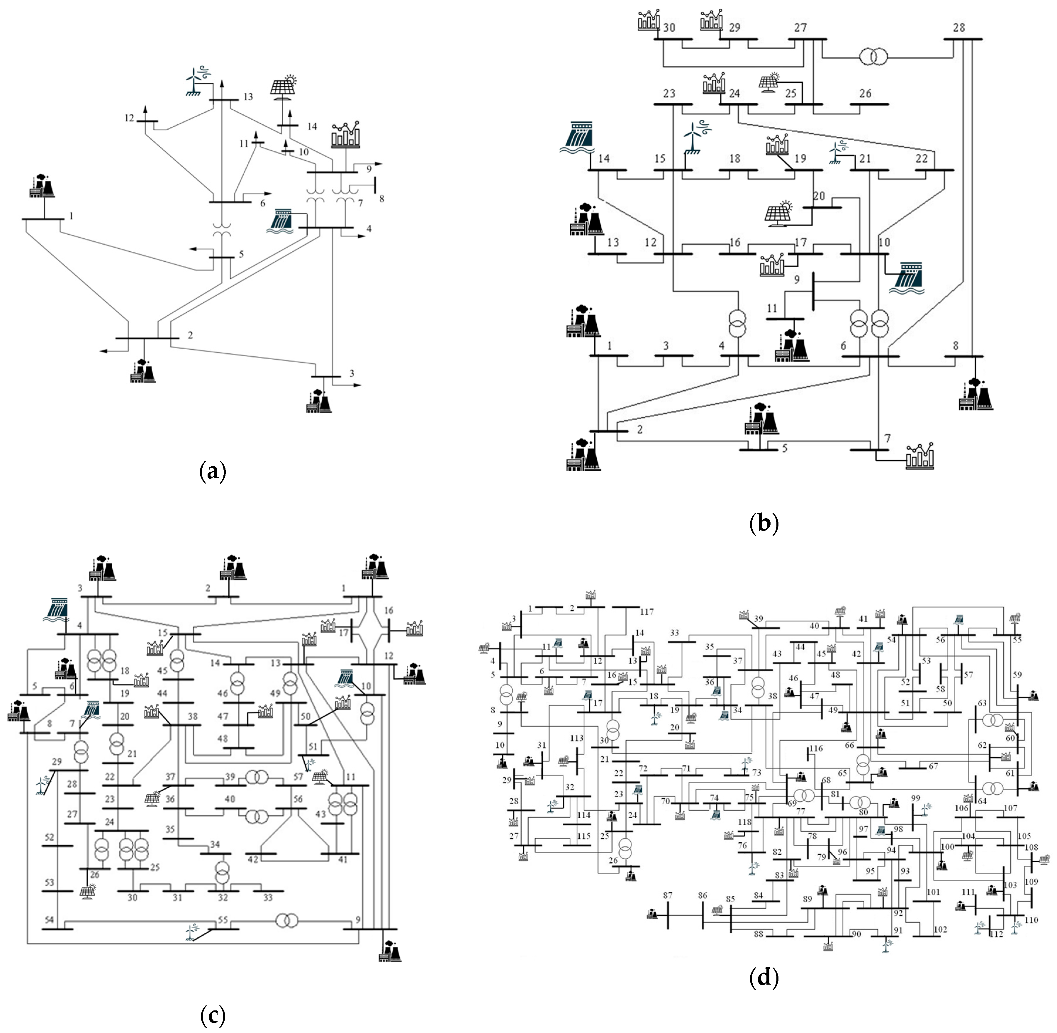
Electrical systems with 14, 30, 57, and 118 buses adapted from the IEEE were analyzed, where renewable generations and demand response resources were inserted. Figure 4 shows the diagram of the electrical systems used in this work. The demand response is represented by the bar graph inserted in the respective bus.

Figure 4. Diagram of the analyzed electrical systems: (a) 14 buses; (b) 30 buses; (c) 57 buses; (d) 118 buses.

3. Evaluation of Case Studies

For the validation of the proposed model, the 14-, 30-, 57-, and 118-bus electrical systems adapted from IEEE were considered, taking into account the presence of loads participating in a demand response program and generators from thermal, wind, photovoltaic, and hydro sources. Figure 4 presents the diagram of the electrical systems used in this work. The demand response is represented by the bar graph inserted in the respective bus.

For the conducted tests, demand response and thermal generation were defined as dispatchable resources, while wind and photovoltaic generators were defined as non-dispatchable, meaning the power generated by these plants follows the immediate availability of the renewable resource. Hydroelectric generation is dispatchable at the base, meaning it has a significantly lower generation cost than other non-dispatchable sources, ensuring the priority generation of this resource.

Two main analyses were conducted. In the first analysis, the impact of the CVaR metrics was verified by varying its parameters in the day-ahead operation scheduling. In the second analysis, a sensitivity analysis of the operation was performed based on the availability of demand response in different system configurations. The simulations were carried out on IEEE standard systems with 14, 30, 57, and 118 buses, and the characteristics of these systems and the simulation results are presented in the following sections.

3.1. Demand Response Resources

The demand response participating in the system operation was defined in the simulations by determining the participating buses in the program, the time interval for load reduction availability, the percentage of potential load reduction relative to the forecasted load, and the price for implementing the load reduction.

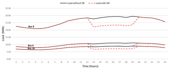
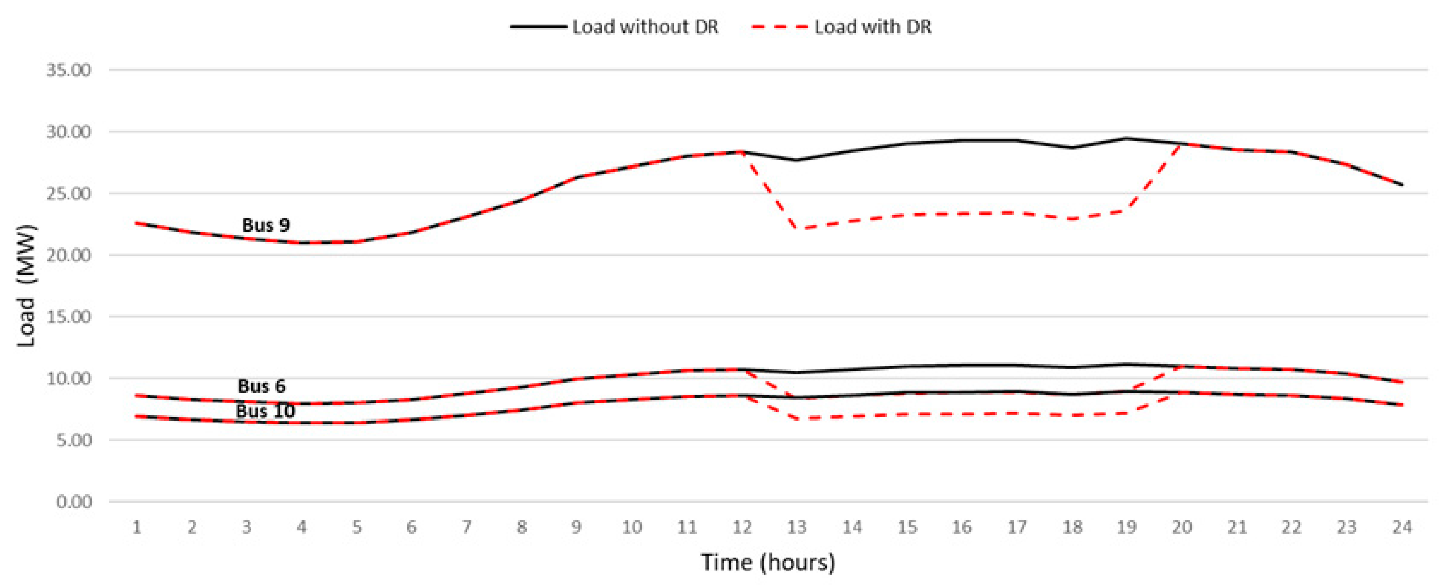
The simulations were conducted considering the demand response resource allocated to specific buses in each system, with an initial reduction potential defined as a percentage of the forecasted load for a 7 h period, from 1:00 p.m. to 8:00 p.m. As an example, Figure 5 illustrates the integration of a 20% demand response resource at 3 buses within the 14-bus system. The demand response price was set as the average of all load reduction offers in the Voluntary Demand Reduction program during October 2021, the last month that the program was in operation, amounting to R$ 153.22/MWh [32].

Figure 5. Loads of the participating buses in the DR with and without demand response in the 14-bus system.

3.2. Generation Resources

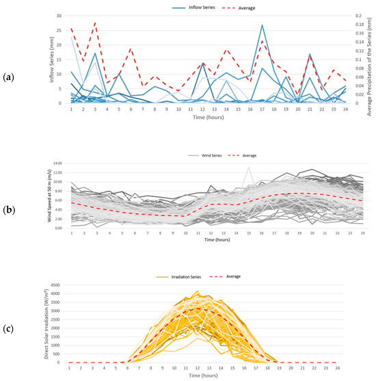
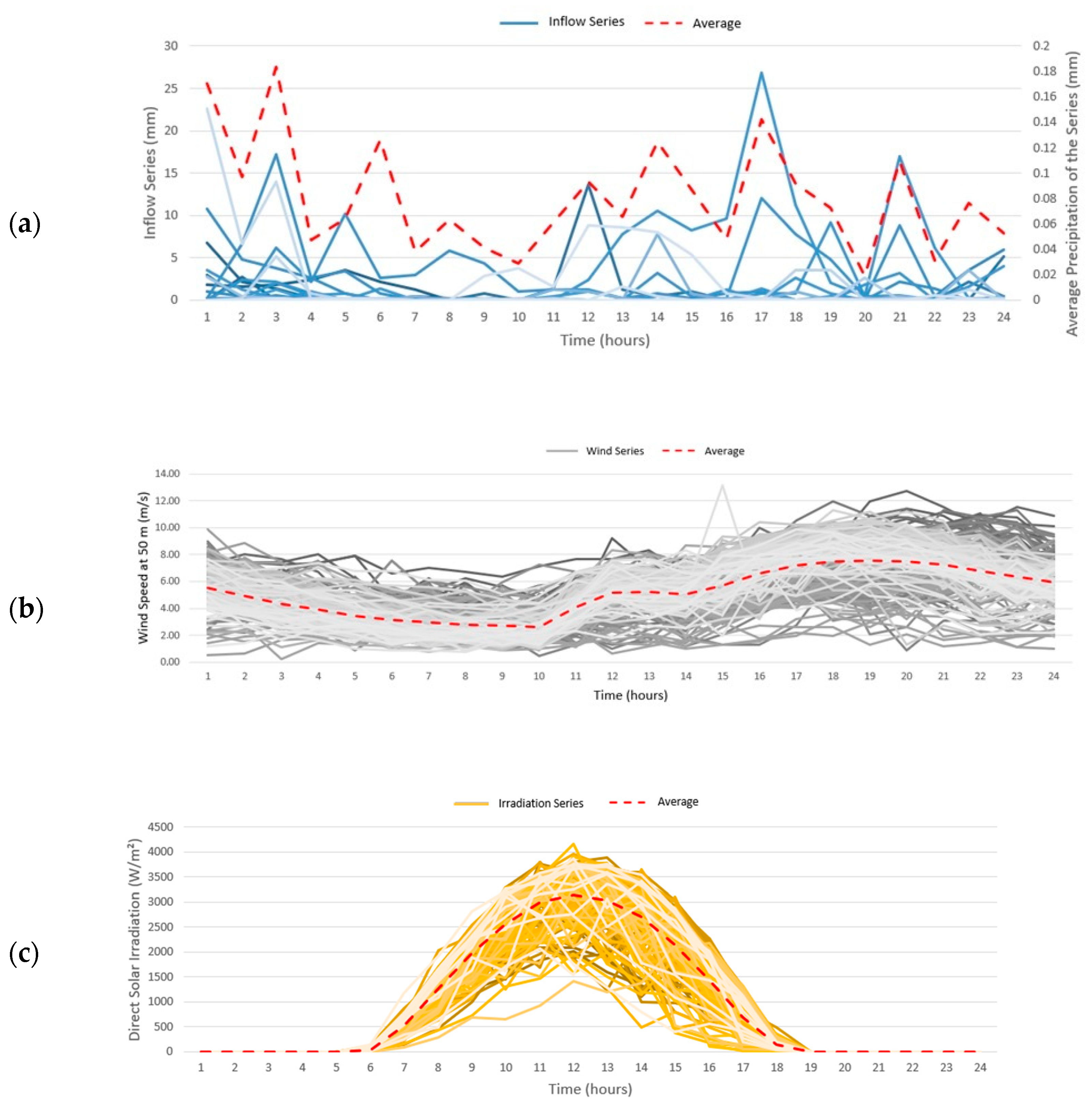
For the buses where wind generation is installed, wind speeds at a 50 m height were considered based on the anemometric measurement data from the Macau/RN weather station for the last ten Januaries, i.e., from January 2014 to January 2023. For the buses where photovoltaic generation is installed, direct irradiations were considered based on the solarimetric measurement data from the Caicó/RN weather station for the last ten Januaries, i.e., from January 2014 to January 2023. In the case of run-of-river hydro generation, the precipitation recorded in the last ten Januaries (January 2014 to January 2023) at the Petrolina/PE weather station available in the INMET BDMEP was considered [33]. Figure 6 illustrates the information regarding the resources for the renewable generation simulations.

Figure 6. Resources for renewable generation simulations: (a) inflow; (b) wind; (c) solar irradiation.

The choice of Macau/RN, Caicó/RN, and Petrolina/PE was due to the fact that these three regions are part of the same electrical subsystem, the Northeast subsystem, which can highlight aspects such as the complementarity between different types of generation at different times.

3.3. CVaR in the Availability of Renewable Resources

The impact of the CVaR methodology on the proposed modeling was tested on all analyzed electrical systems. This risk methodology was applied to the renewable resource forecasts for the day-ahead operation.

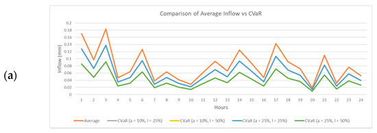
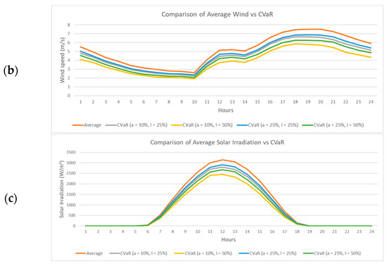
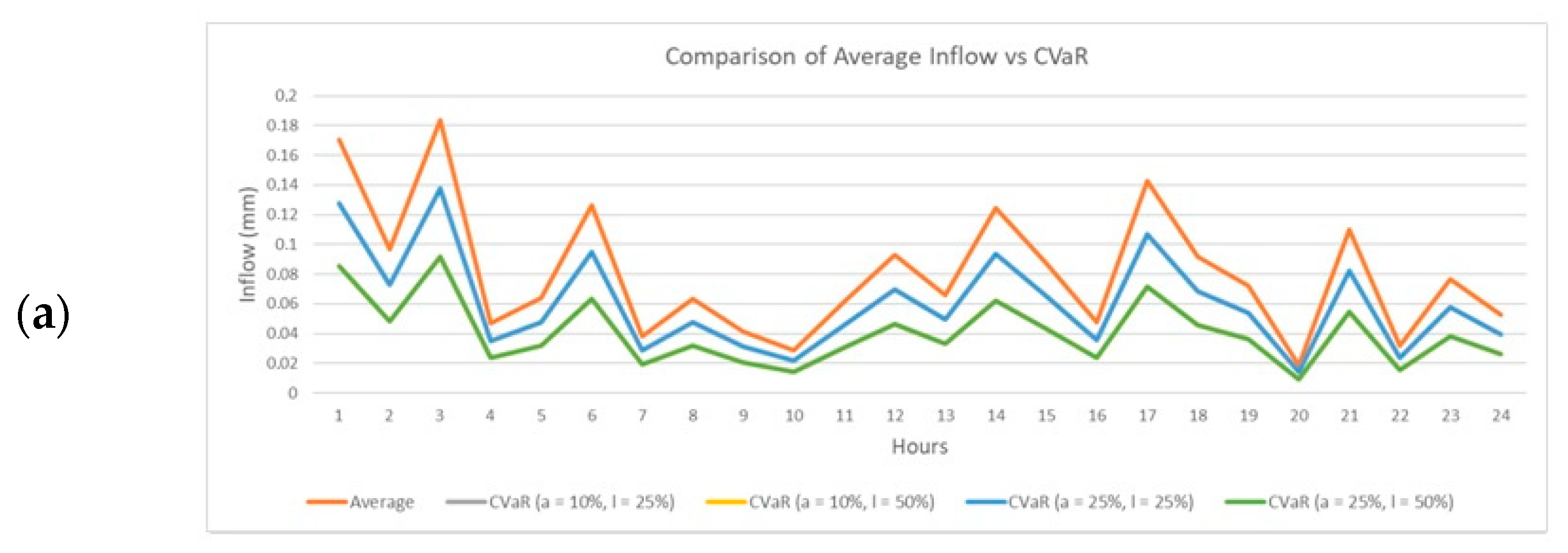
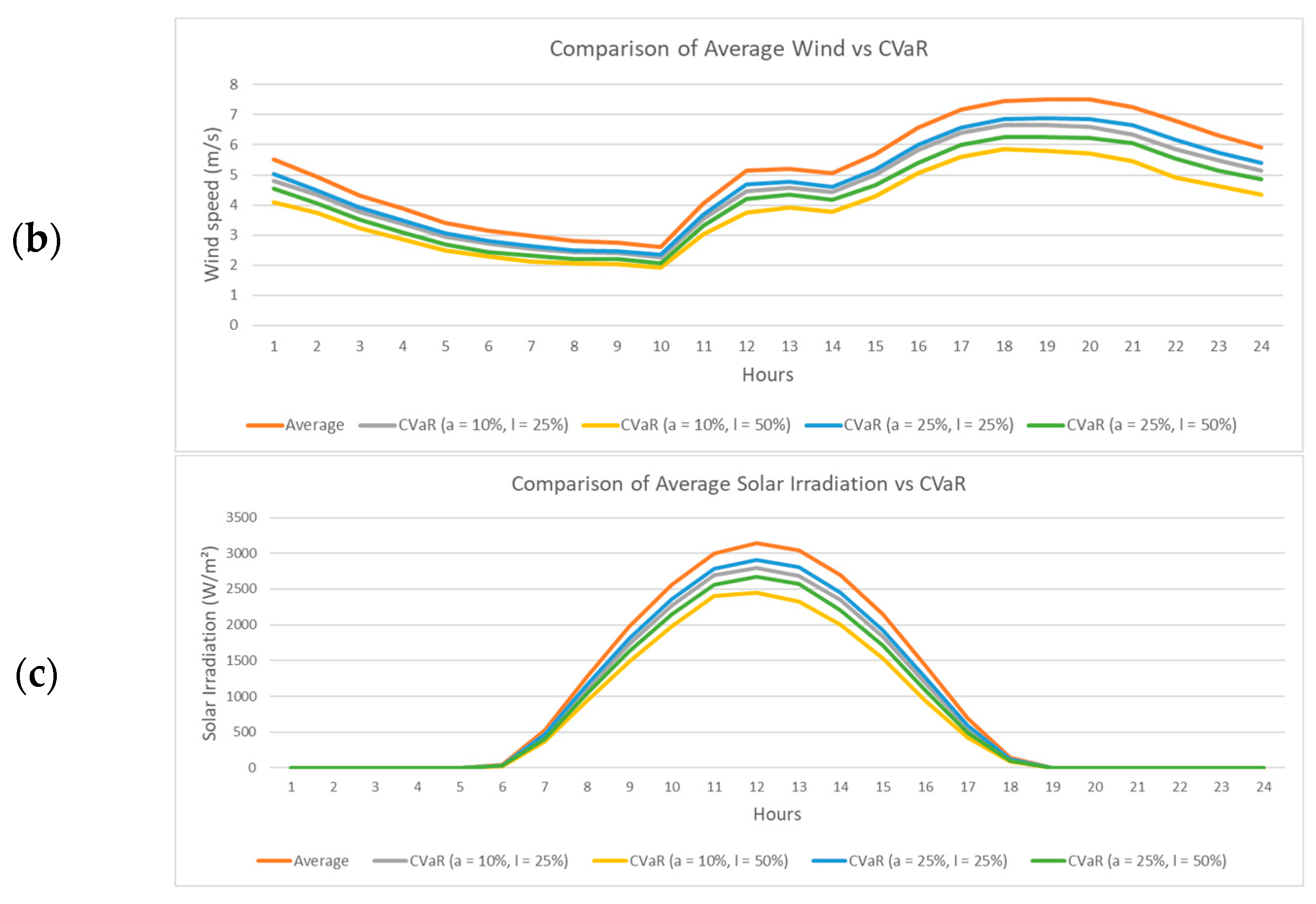
Figure 7 illustrates the behavior of applying CVaR to renewable resources compared to the average over the analysis horizon. It can be observed that for all cases there was a reduction in resources relative to the average curve, which was expected since this risk criterion assigns higher weights to the worst scenarios to maintain the security of the electrical system.

Figure 7. Comparison of renewable resource vs. CVaR. (a) Inflow; (b) wind; (c) solar irradiation.

The result obtained for the application of CVaR in climatic time series varied significantly among the different types of renewable resources analyzed, being more imprecise for the hydro resource. This imprecision was evidenced, for example, in the application of CVaR with the parameter pairs α = 10%/λ = 25% and α = 25%/λ = 25% which resulted in exactly the same outcomes, as well as in the application of the parameter pairs α = 10%/λ = 50% and α = 25%/λ = 50% which also presented the same results among them (Figure 6a). Thus, it was observed that CVaR has a more robust and pertinent applicability in wind and solar irradiation series, as there is availability of these resources for most of the time. In contrast, when considering rainfall series, the dynamics become more challenging, as the worst days in the analyzed series are those with no rain, resulting in zero values for this resource. This phenomenon limits the effectiveness of CVaR in managing risks associated with variability in rainfall series, making it necessary to explore alternative approaches or combinations of risk metrics to better capture the complexity of these specific climatic patterns.

3.4. CVaR in the Operations of Case Studies

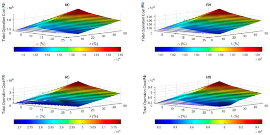
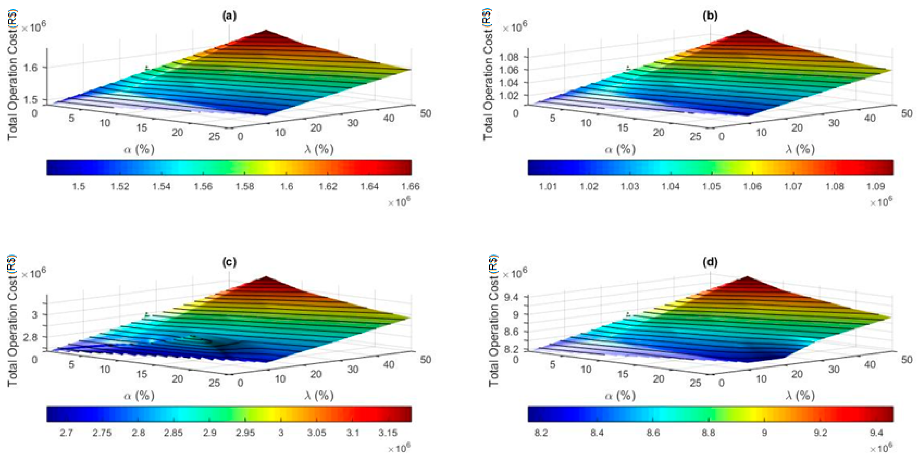
Simulations for each of the systems were performed for 26 different scenarios, where the first scenario does not consider the application of CVaR and the subsequent scenarios are formed by applying CVaR with varying parameters α and λ. All scenarios were simulated considering a 20% demand response potential at each of the buses that have this resource. The parameter α was tested from 0% to 25% in 5% increments, while the parameter λ was tested from 0% to 50% in 10% increments between scenarios. The base scenario did not apply the CVaR methodology in the simulation. Figure 8 illustrates the simulated total operational cost considering CVaR for the tested systems.

Figure 8. Simulated total operation cost considering CVaR for the systems: (a) 14 buses; (b) 30 buses; (c) 57 buses; (d) 118 buses.

Regarding Figure 8, it can be observed that the total operational cost was lower in the baseline scenario where CVaR was not applied. In these scenarios, the renewable resources for the operation were considered according to the average. After applying CVaR, these resources were reduced to prepare the day-ahead operation more securely concerning the dependence on intermittent generation.

The largest increase in the average operation cost occurred in the scenario with CVaR applied with parameters α and λ of 5% and 50%, respectively, for all analyzed systems. For the 14-, 30-, 57-, and 118-bus systems, the increase compared to the base scenario with CVaR applied with these parameters was 11.80%, 8.85%, 19.28%, and 16.09%, respectively.

The electrical losses showed small variations for the 14-, 30-, and 118-bus systems, with standard deviations between the scenarios of 0.5497 MWh, 0.7408 MWh, and 3.5686 MWh, respectively. The largest variation in electrical losses among the scenarios occurred for the 57-bus system, presenting a standard deviation between the scenarios of 10.4031 MWh.

From a system security perspective, the more thermal generation is incorporated into the system planning, the greater the security, as this type of source does not face intermittency issues. In scenarios where CVaR is not applied, the dispatched thermal generation is 3.130 GWh, 3.993 GWh, 17.229 GWh, and 49.849 GWh for the 14-, 30-, 57-, and 118-bus systems, respectively. When CVaR is applied with parameters α and λ set at 5% and 50%, the dispatched thermal generation increases to 3.638 GWh, 4.309 GWh, 27.281 GWh, and 53.739 GWh, respectively.

In all simulated scenarios for the 14-, 30-, and 57-bus systems, the demand response resources were fully dispatched. In the 118-bus system, the total maximum demand response resource for the 24 h was 1543.10 MWh. This resource was not fully dispatched in any of the scenarios. The highest demand response dispatch was 1454.25 MWh and occurred in the scenario with α and λ of 5% and 50%, respectively, which was the scenario with the highest operational cost.

3.5. Analysis of Demand Response in Case Studies

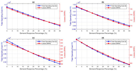
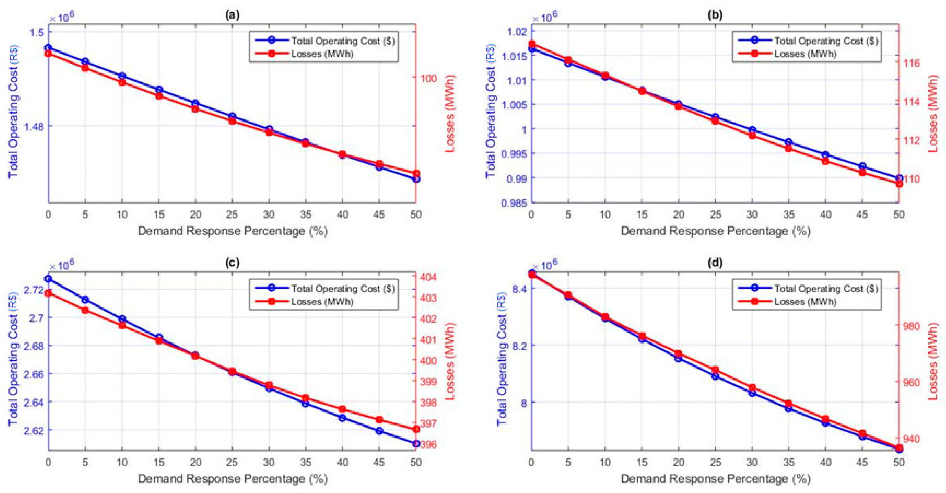
A sensitivity analysis was conducted where the amount of demand response available at each of the participating buses in the system was varied from 0% to 50% to analyze the impact on the system operation costs. The main results of the sensitivity analysis of the amount of demand response participating in the system for all analyzed systems are presented in Figure 9.

Figure 9. Simulated total operation cost and losses considering different DR scenarios for the systems: (a) 14 buses; (b) 30 buses; (c) 57 buses; (d) 118 buses.

From the obtained results, it was possible to observe some relevant points regarding the sensitivity of demand response for the day-ahead system operation. The total operation cost was reduced in all scenarios as the availability of demand response increased. The cost reduction due to the increase in DR in the system is non-linear, given the non-linearity of the generation costs of thermal power plants.

The reduction in operation cost for the 14-, 30-, 57-, and 118-bus systems was 1.87%, 2.60%, 2.00%, and 3.53%, respectively, compared to the scenario without DR for the scenario with 50% DR.

The increase in DR resulted in a reduction in system load, with this reduction from the scenario without DR to the scenario with 50% DR being 2.99%, 3.46%, 2.70%, and 4.09% for the 14-, 30-, 57-, and 118-bus systems, respectively.

The increase in DR resulted in a reduction in electrical losses due to the reduction in power flows on the lines in all analyzed scenarios. This reduction from the scenario without DR to the scenario with 50% DR was 4.03%, 6.20%, 1.62%, and 6.13% for the 14-, 30-, 57-, and 118-bus systems, respectively.

Demand response in the simulated scenarios proved to be an important resource for reducing operation costs and losses and increasing the security of the electrical system.

4. Conclusions

This work presented a new approach to the demand response program based on the modeling of an optimal power flow problem considering the presence of intermittent renewable generation. The objective function of the problem was to minimize the operational cost over a 24 h horizon, resembling the day-ahead operation planning problem.

In the mathematical modeling of the problem, in addition to thermal sources, run-of-river hydro, wind, and solar generation were also considered. Each source had its specific generation curve modeled based on the availability of its respective natural resource, and the uncertainty of generation was considered through the application of the CVaR risk methodology. The inherent constraints of the electrical system were considered in the problem modeling, such as power balance constraints and transmission line flow limits.

For the validation of the proposed model, data from meteorological stations in northeast Brazil were used, such as inflow, wind, and solar irradiation data, which were input into standard IEEE test systems of 14, 30, 57, and 118 buses. The computational modeling was developed in the AMPL environment, and the MINOS solver was used to solve the problem.

Two different analyses were conducted in this work. The first was the analysis of the impact of CVaR on the day-ahead operation planning, and the second was the sensitivity analysis of demand response in the analyzed systems.

The application of CVaR to the expectation of renewable resources was important to signal to the system operator the need to schedule more thermal generation for the day-ahead operation to increase security against the uncertainties of resource intermittency, which implies an increase in the system operating cost. Additionally, it was identified that this methodology has better applicability to wind and solar irradiation series, as there is a better-defined pattern within the month for these types of resources, which does not occur with rainfall series since there is no precipitation for most days in the study location. Regarding the CVaR parameters α and λ, it was evident that operating costs are higher as α is reduced and λ is increased. The most significant rise in average operational costs was observed in the scenario where CVaR was applied with α and λ parameters set at 5% and 50%, respectively, across all analyzed systems. In the 57-bus system, this cost increase peaked at 19.28%.

In the simulations of the demand response sensitivity analysis, the importance of demand response in systems with a strong penetration of renewable resources was evidenced in terms of reducing operation costs, losses, and increasing system security. There is a direct, yet non-linear, relationship between the increase in demand response in the system and the reduction in operation costs. The reduction in operating cost reached up to 3.53%, with a decrease in losses of 4.09% for the 118-bus system with a 50% DR.

Based on the tests conducted and the results obtained, it is possible to affirm that the proposed modeling met its objective and proved to be efficient in solving the linearized optimal power flow problem with losses under the conditions evaluated in this work.

References

- Albadi, M.H.; El-Saadany, E.F. Demand response in electricity markets: An overview. In Proceedings of the 2007 IEEE Power Engineering Society General Meeting, Tampa, FL, USA, 24–28 June 2007. [Google Scholar]
- Tracking Demand Response. Available online: https://www.iea.org/energy-system/energy-efficiency-and-demand/demand-response (accessed on 20 April 2024).
- Duan, Q. A price-based demand response scheduling model in day-ahead electricity market. In Proceedings of the 2016 IEEE Power and Energy Society General Meeting (PESGM), Boston, MA, USA, 17–21 July 2016; pp. 1–5. [Google Scholar]
- Firouz, M.H.; Alemi, A. Optimal energy and reserve scheduling of wind power producers in electricity market considering demand response. In Proceedings of the 2016 IEEE International Conference on Power and Energy (PECon), Melaka, Malasia, 28–29 November 2016; pp. 652–656. [Google Scholar]
- Roald, L.A.; Pozo, D.; Papavasiliou, A.; Molzahn, D.K.; Kazempour, J.; Conejo, A. Power systems optimization under uncertainty: A review of methods and applications. Electr. Power Sysemst Research 2023, 214 Pt A, 108725. [Google Scholar] [CrossRef] [Scilit]
- Singh, N.K.; Koley, C.; Gope, S. Effect of Energy Storage Systems on Economic Risk Values in Wind Energy Integrated Power System. In Proceedings of the IEEE 4th Annual Flagship India Council International Subsections Conference (INDISCON), 2023, Mysore, India, 5–7 August 2023; pp. 1–6. [Google Scholar]
- Singh, N.K.; Koley, C.; Gope, S.; Dawn, S.; Ustun, T.S. An Economic Risk Analysis in Wind and Pumped Hydro Energy Storage Integrated Power System Using Meta-Heuristic Algorithm. Sustainability 2021, 13, 13542. [Google Scholar] [CrossRef] [Scilit]
- Singh, N.K.; Koley, C.; Gope, S. Wind Energy and Pumped Hydro Storage Integrated Power System Risk Analysis using VaR and CvaR. In Proceedings of the Second International Conference on Next Generation Intelligent Systems (ICNGIS), Kottayam, India, 29–31 July 2022; pp. 1–5. [Google Scholar]
- Jiang, J.; Kou, Y.; Bie, Z.; Li, G. Optimal Real-Time Pricing of Electricity Based on Demand Response. Energy Procedia 2019, 159, 304–308. [Google Scholar] [CrossRef] [Scilit]
- Heydarian-Forushani, E.; Golshan, M.E.H.; Shafie-khah, M.; Catalão, J.P.S. A comprehensive linear model for demand response optimization problem. Energy 2020, 209, 118474. [Google Scholar] [CrossRef] [Scilit]
- Sun, S.; Cheng, Y.; Xing, J.; Yu, P.; Wang, Y. Day-ahead optimization of integrated electricity and thermal system combining multiple types of demand response strategies and situation awareness technology. Front. Energy Res. 2024, 12, 1337169. [Google Scholar] [CrossRef] [Scilit]
- Luo, Q.; Zhang, S. Two-stage Optimal Scheduling of Virtual Power Plant Considering Demand Response and Forecast Errors. In Proceedings of the 4th International Conference on Electrical Engineering and Control Technologies (CEECT), Shanghai, China, 16–18 December 2022; pp. 852–856. [Google Scholar]
- Lu, Z.; Lu, S.; Xu, M.; Bowen, C. A robust stochastic stability analysis approach for power system considering wind speed prediction error based on Markov model. Comput. Stand. Interfaces 2021, 75, 103503. [Google Scholar] [CrossRef] [Scilit]
- Arun, C.; Aswinraj, R.; Bijoy, M.T.; Micky, R.R. Day Ahead Demand Response Using Load Shifting Technique in Presence of Increased Renewable Penetration. In Proceedings of the IEEE 7th International conference for Convergence in Technology (I2CT), Mumbai, India, 7–9 April 2022. [Google Scholar]
- Kang, J.; Lee, S. Data-Driven Prediction of Load Curtailment in Incentive-Based Demand Response System. Energies 2018, 11, 2905. [Google Scholar] [CrossRef] [Scilit]
- Miraftabzadeh, S.M.; Foiadelli, F.; Longo, M.; Pasetti, M. A Survey of Machine Learning Applications for Power System Analytics. In Proceedings of the IEEE International Conference on Environment and Electrical Engineering and IEEE Industrial and Commercial Power Systems Europe (EEEIC/I&CPS Europe), Genova, Italy, 11–14 June 2019; pp. 1–5. [Google Scholar]
- Khaloie, H.; Dolanyi, M.; Toubeau, J.; Vallée, F. Review of Machine Learning Techniques for Optimal Power Flow. SSRN 2014. [Google Scholar] [CrossRef] [Scilit]
- Hosseini-Firouz, M.; Alemi, A.; Alefy, B. Unit Commitment Model under Uncertainty of Wind Power Producer. Iran. J. Sci. Technol. Trans. Electr. Eng. 2021, 45, 1295–1309. [Google Scholar] [CrossRef] [Scilit]
- Gong, H.; Wang, H. A stochastic generation scheduling model for large-scale wind power penetration considering demand-side response and energy storage. In Proceedings of the China International Conference on Electricity Distribution (CICED), Xi’an, China, 10–13 August 2016; pp. 1–6. [Google Scholar]
- Jabr, R.A. Distributionally Robust CVaR Constraints for Power Flow Optimization. IEEE Trans. Power Syst. 2020, 35, 3764–3773. [Google Scholar] [CrossRef] [Scilit]
- Zaforteza, M.E. Demand Response Participation in Different Markets in Europe. Master’s Thesis, Tampere University, Tempere, Finland, 2019. Available online: https://trepo.tuni.fi/handle/10024/115813 (accessed on 24 August 2024).
- Zhang, J.; Wang, J.; Yue, C. Small Population-Based Particle Swarm Optimization for Short-Term Hydrothermal Scheduling. IEEE Trans. Power Syst. 2011, 27, 142–152. [Google Scholar] [CrossRef] [Scilit]
- Soroudi, A. Power System Optimization Modeling in GAMS, 1st ed.; Springer: Dublin, Ireland, 2017; pp. 78–93. [Google Scholar]
- Monticelli, A.J.; Garcia, A. Introdução a Sistemas de Energia Elétrica, 2nd ed.; Editora Unicamp: Campinas, Brazil, 2011; pp. 209–211. [Google Scholar]
- Artzner, P.; Delbaen, F.; Eber, J.M.; Heath, D. Coherent Measures of Risk. Math. Financ. 1999, 9, 203–228. [Google Scholar] [CrossRef] [Scilit]
- Souza, R.V.X.S. Análise dos Impactos de Políticas de Resposta da Demanda na Formação do Preço da Liquidação das Diferenças no Mercado de Energia Elétrica Brasileiro. Master’s Thesis, University of ABC, Santo André, Brazil, 2014. Available online: https://biblioteca.ufabc.edu.br/index.php?codigo_sophia=76743 (accessed on 24 August 2024).
- Halkos, G.E.; Tsirivis, S.T. Value-at-risk methodologies for effective energy portfolio risk management. Econ. Anal. Policy 2019, 62, 197–212. [Google Scholar] [CrossRef] [Scilit]
- Ramos, D.S. Price Formation in Short and Long Term Markets. In Pricing and Commercialization of Electric Energy II Course; Graduate Program in Electrical Engineering, Department of Electric Energy and Automation Engineering, University of Sao Paulo: São Paulo, Brazil, 2013. (In Portuguese) [Google Scholar]
- Bendrinana, M.F.; Rider, M.J.; Castro, C.A. Ill-conditioned Optimal Power Flow solutions and performance of non-linear programming solvers. In Proceedings of the 2009 IEEE Bucharest PowerTech, Bucharest, Romania, 28 June–2 July 2009; pp. 1–7. [Google Scholar]
- Bixby, R.E. A Brief History of Linear and Mixed-Integer Programming Computation. Doc. Math. 2012, 107–121. [Google Scholar]
- Murtagh, B.A.; Saunders, M.A. MINOS 5.5 User’s Guide. Stanford University, Stanford, United States of America, 2003. Available online: https://web.stanford.edu/group/SOL/guides/minos551.pdf (accessed on 30 April 2024).
- CCEE–Câmara de Comercialização de Energia Elétrica. Relatório de Atendimento ao Programa de Redução Voluntária da Demanda–Contabilização de Outubro/2021. São Paulo, Brasil, 2021. Available online: https://www.ccee.org.br/pt/web/guest/-/co-ccee-disponibiliza-resultados-contabilizados-de-calculos-dos-efeitos-do-mecanismo-de-reducao-voluntaria-da-demanda (accessed on 24 August 2024).
- INMET–Instituto Nacional de Meteorologia. Banco de Dados Meteorológicos. Brasília, Brasil, 2023. Available online: https://bdmep.inmet.gov.br/ (accessed on 26 March 2023).
Disclaimer/Publisher’s Note: The statements, opinions and data contained in all publications are solely those of the individual author(s) and contributor(s) and not of MDPI and/or the editor(s). MDPI and/or the editor(s) disclaim responsibility for any injury to people or property resulting from any ideas, methods, instructions or products referred to in the content. |
© 2024 by the authors. Licensee MDPI, Basel, Switzerland. This article is an open access article distributed under the terms and conditions of the Creative Commons Attribution (CC BY) license (https://creativecommons.org/licenses/by/4.0/).