Predictive Model Based on Machine Learning to Determine Gold Price Fluctuation and Improve Trading Decisions

Abstract

Gold’s price reflects currency, opportunity-cost, and safe-haven channels whose strength shifts across regimes, motivating an empirical, data-driven forecasting approach. This study develops a monthly gold price forecasting system for ASM sales-timing decisions in Peru (January 2020–June 2026) using macro-financial predictors including a geopolitical risk index and three U.S. monetary indicators, none of which were Granger-causal and were therefore excluded from the production set. After confirming non-stationarity and Johansen cointegration (four vectors), thirty-two model-feature-set combinations, including Elastic Net, Bayesian Ridge, and a PCA factor, were compared under strict temporal validation with bounded hyperparameter search. The selected model, Ridge regression on the CONTROL feature set, achieved a cross-validation MAPE of 2.29% and test MAPE of 3.62% (official)/3.15% (extended sensitivity window). It was benchmarked against random walk, historical mean, and exponential smoothing and evaluated via the Diebold–Mariano, Clark–West, encompassing, and Model Confidence Set tests (low-power caveats given the small sample). A dual-horizon Monte Carlo simulation, robust to heavy-tailed shocks, projected USD 4482/oz (December 2026) and USD 5106/oz (December 2027). A sales-timing backtest showed a statistically significant result (−0.67%) versus a passive strategy, indicating calibrated price information alone does not yet yield a reliable trading edge, supporting the model’s role as decision support rather than an autonomous trading signal.

1. Introduction

Gold occupies a singular position in the global economic system, functioning simultaneously as a commodity, a monetary reserve asset, and a safe-haven instrument. Its price reflects complex interactions among macroeconomic variables, financial market dynamics, and geopolitical factors, which makes accurate forecasting a persistent challenge for both academic research and industry practice. In the Peruvian context, this challenge carries concrete economic consequences: gold is the country’s second most important export commodity, with 99.7 metric tons produced in 2023 and record export revenues of USD 12,688 million in 2024, a 49% increase over the previous year (BCRP, 2025). According to Salazar Herrada (2024), Peruvian gold exports recorded a 32% increase in the first half of 2024 alone, driven primarily by the escalation of international prices. By mid-2026, the international price had moved into the USD 4500–5000/oz range, an unprecedented level that generates substantial volatility and particularly affects artisanal and small-scale mining (ASM) operations, which account for approximately 40% of national production (Rumbo Minero, 2024). According to CooperAccion (2024), small-scale enterprises in regions such as Puno lack specialized predictive tools and rely on empirical judgment to decide when to commercialize their output, generating suboptimal sales-timing decisions that directly affect their economic profitability.

The application of machine learning (ML) algorithms to commodity price forecasting offers a promising avenue for addressing this problem (Sandoval, 2019). Varian (2014) frames this broader shift toward data-rich, algorithm-based methods in applied econometrics generally. A substantial body of literature has demonstrated the effectiveness of these algorithms for gold price prediction. Villada et al. (2016) showed that artificial neural networks outperform traditional econometric models; Sadorsky (2021) demonstrated that tree-based classifiers, including Random Forest, achieve 78.4% accuracy for directional gold price prediction; Foroutan and Lahmiri (2024) compared deep learning architectures for crude oil and precious metals and reported that recurrent and hybrid models can attain very low error rates under favorable sampling conditions, while also documenting that performance deteriorates sharply when training samples are small and validation is not strictly out-of-sample. Liang et al. (2022) proposed a hybrid ICEEMDAN-LSTM-CNN-CBAM model with results superior to univariate approaches; Khani et al. (2021) demonstrated the robustness of deep learning for gold price forecasting even under pandemic-distorted market conditions; and Wagh et al. (2022) and Ghule and Gadhave (2022) confirmed the practical utility of ML models for short-horizon gold price prediction. In the Latin American context, Castillo (2022) achieved high predictive accuracy using SVR and regression trees for the mining industry; Jimenez Falcón (2025) reported very high in-sample fit for Linear Regression applied to mineral price prediction; and Cotrina-Teatino et al. (2025) demonstrated the feasibility of ML algorithms in the context of Peruvian mining exploration. Ramirez Martínez (2017) identified the US Dollar Index, real interest rates, and stock market volatility as influential determinants of gold price, while Tebin and James (2022) and Cohen and Aiche (2023) confirmed that macroeconomic and financial variables are robust predictors of commodity returns. More recent work has extended this determinant set to include measures of geopolitical tension and monetary policy stance: Caldara and Iacoviello (2022) show that news-based geopolitical risk depresses investment and raises the probability of macroeconomic disasters, while Medeiros et al. (2021) document that tree-based and penalized ML models incorporating a large panel of monetary and real-activity indicators systematically outperform simple benchmarks in U.S. inflation forecasting, motivating the inclusion of a geopolitical risk index and monetary indicators (CPI, the federal funds rate, and M2) as candidate predictors in the present study (Section 3.5).

Beyond algorithm selection, a growing body of econometric and empirical-finance literature emphasizes that the statistical properties of the underlying series fundamentally constrain how ML models for asset prices should be built and evaluated. Financial price levels are typically integrated of order one, I(1), and regressions performed directly on non-stationary levels risk producing spurious relationships (Hamilton, 1994; Brockwell & Davis, 2016); the standard remedy is to model returns or first differences, whose stationarity can be verified with unit-root tests such as the Augmented Dickey–Fuller and Kwiatkowski–Phillips–Schmidt–Shin tests (Tsay, 2010). When several non-stationary series share a long-run equilibrium relationship, that relationship is itself informative and should not be discarded; the Engle and Granger (1987) and Johansen (1991) cointegration frameworks formalize this insight and have become standard tools in commodity-and-macro-asset modeling. This cointegration evidence is not presented in this study as a prerequisite for the ML forecasting exercise, which does not rely on the distributional assumptions of classical time-series econometrics; rather, it is reported as complementary evidence of the market’s long-run equilibrium structure, contextualizing the short-horizon, return-based ML approach adopted here and motivating a vector error-correction (VECM) extension as future research (Section 6). Classical time-series benchmarks—ARIMA models (Box et al., 2015) and GARCH-family volatility models (Bollerslev, 1986)—remain useful reference points against which the incremental value of ML approaches can be assessed (Diebold, 2015), even when, as in the present study, an ARIMA specification proves too unstable to serve as a forecasting benchmark and is retained only as a documented diagnostic. On the ML side, Hastie et al. (2009) and Gu et al. (2020) provide the statistical-learning foundations for tree-based ensembles and regularized regression in asset-pricing applications, while Kelly et al. (2019) show that characteristic-based, interpretable models can rival more complex architectures. Bauer and Hamilton (2018) further show that inference about which predictors genuinely carry information beyond a persistent baseline is subject to serious small-sample distortions in return-predictive regressions, a caution that directly informs the robustness checks (Clark–West and bootstrap-based) introduced in Section 3.9 and Section 4.6. Zhang et al. (1998) and Makridakis et al. (2020), summarizing the M3 and M4 forecasting competitions, caution that simple, well-validated models frequently outperform more complex ones once leakage-free, expanding-window evaluation is enforced—an observation directly relevant to the comparison between the ARIMA/LSTM alternatives considered and the tree-based ensembles ultimately selected in this study. Makridakis et al. (2022), summarizing the subsequent M5 competition, confirm this pattern in a large-scale retail-forecasting setting, and additionally highlight the value of hierarchical and probabilistic evaluation, both of which inform the uncertainty quantification introduced in Section 3.10.

Despite this rich literature, a gap persists: no study has developed an ML predictive model for gold prices that (a) explicitly tests for non-stationarity and long-run cointegration before modeling short-run dynamics, (b) enforces a strictly temporal train/test partition with expanding-window cross-validation to avoid look-ahead bias, (c) screens candidate predictors through formal Granger-causality tests rather than raw correlation, (d) produces forecasts in log-return space with a bounded, simulation-based uncertainty band rather than an unconditional level extrapolation, and (e) applies the resulting model with an explicit focus on optimizing commercial sales timing for Peruvian artisanal and small-scale mining while quantifying its implications for enterprise profitability; this research addresses that gap directly.

The quantitative design adopted throughout this study is grounded in the economic reasoning set out above rather than pursued as an end in itself. Each candidate predictor is included because it maps to an identifiable economic channel through which gold prices are understood to move (the currency channel via the US Dollar Index, the opportunity-cost channel via real and nominal interest rates, the risk-appetite channel via equity markets and the VIX, and the monetary and geopolitical channels examined in Section 2.1), and the Granger-causality and cointegration tests applied in Section 3.4 and Section 3.5 serve to confirm, rather than assume, that these channels carry measurable predictive or long-run information over the present sample. Where the quantitative evidence and a predictor’s theoretical role diverge, as with the geopolitical and monetary indicators discussed in Section 2.1, that divergence is itself economically informative and is discussed as such rather than treated as a purely statistical outcome.

2. Literature Review and Theoretical Framework

2.1. Determinants of Gold Price and Its Time-Series Properties

The dynamics of gold prices are determined by a heterogeneous set of macroeconomic, financial, and geopolitical forces. The US dollar maintains an inverse relationship with gold, since a weaker dollar makes gold cheaper for holders of other currencies and tends to push prices upward (Diaz-Hernandez et al., 2020). Real interest rates represent the opportunity cost of holding a non-yielding asset such as gold, so that lower or negative real rates typically support higher prices (Ramirez Martínez, 2017). Equity-market dynamics, captured here through the S&P 500, interact with gold in a regime-dependent manner. Geopolitical tension and monetary policy stance constitute two further determinants that this research incorporates explicitly. Caldara and Iacoviello (2022) construct a monthly, news-based Geopolitical Risk (GPR) index and show that elevated geopolitical risk is associated with lower investment and a higher probability of adverse macro-financial outcomes, a channel plausibly relevant to gold’s role as a safe-haven asset. On the monetary side, the consumer price index (CPI), the effective federal funds rate, and the M2 money supply jointly proxy the inflationary and liquidity conditions that theory (Ramirez Martínez, 2017) and recent ML-based inflation-forecasting evidence (Medeiros et al., 2021) identify as first-order drivers of gold’s relative attractiveness as a store of value. Section 3.5 subjects all three monetary series and the GPR index to the same Granger-causality and multicollinearity screening applied to the original thirteen candidates.

Beyond these individual channels, a broader literature on gold as an asset class provides context that directly shapes several methodological choices made in this study. O’Connor et al. (2015), surveying the financial economics of gold, document that gold’s behavior as a hedge or safe-haven asset relative to inflation, currencies, and equities is empirically time-varying rather than a fixed structural relationship, and that the relative importance of demand- and supply-side determinants shifts across market regimes and has not been conclusively resolved by the existing literature. This finding motivates estimating the relationships examined here empirically, through Granger causality and machine learning, rather than imposing a fixed theoretical functional form a priori. Erb and Harvey (2013) show, further, that the real price of gold has historically reverted toward its long-run mean following periods of elevated valuation, and that the popular narrative of gold as a reliable, constant inflation hedge is not well supported over practical investment horizons. This mean-reversion evidence directly informs the Monte Carlo specification in Section 3.10: the zero-drift scenario is adopted as the primary forecasting assumption, and the historical-drift scenario, which would implicitly assume that the elevated returns observed toward the end of the sample continue unabated, is reported only as a sensitivity check rather than as the central forecast, precisely because Erb and Harvey’s (2013) evidence counsels against extrapolating recent elevated real gold returns into the future.

2.2. Machine Learning Approaches to Financial Forecasting

Random Forest (Breiman, 2001) constructs multiple decision trees on bootstrap samples of the training data and averages their predictions, reducing variance relative to a single tree while retaining the capacity to model non-linear interactions among predictors without requiring an explicit functional form. Gradient boosting methods (XGBoost 3.3.0, LightGBM 4.6.0) build trees sequentially, each correcting the residual error of the ensemble so far and typically achieve strong in-sample fit at the cost of a higher risk of overfitting on small samples (Hastie et al., 2009). Regularized linear methods (Ridge and, in this revision, Elastic Net and Bayesian Ridge) penalize coefficient magnitude to control variance in the presence of correlated predictors, which is particularly relevant given the moderate-to-high correlation observed among several commodity and macro-financial series (Section 3.6). Elastic Net combines the L1 and L2 penalties of Lasso and Ridge, while Bayesian Ridge places a probabilistic prior over the regression coefficients and yields a natural, model-based measure of predictive uncertainty; both serve as additional, low-risk model families that extend the benchmark set without the overfitting risk associated with more heavily parameterized alternatives such as regime-switching or state-space models under the present sample size (Section 3.6 and Section 6). A principal-component diffusion-index specification (Stock & Watson, 2002), which summarizes the co-movement of the full commodity-and-macro panel in a single factor, is evaluated alongside these models as a simplified, low-dimensional proxy for a full dynamic-factor model.

2.3. Machine Learning in Data-Rich Macro-Financial Environments

A parallel and rapidly growing literature applies ML methods specifically to macro-financial forecasting with many predictors, a setting structurally similar to the present gold price problem. Varian (2014) provides an accessible overview of decision trees, regularization, and cross-validation for economists confronting large predictor sets. Stock and Watson (2002) formalize the diffusion-index (principal-component) approach used in this revision’s FACTOR specification (Section 3.6), showing that a small number of estimated factors can summarize the forecasting-relevant information in a large macroeconomic panel. Medeiros et al. (2021) compare a wide range of ML and penalized-regression models for U.S. inflation forecasting and find that Random Forest, applied to a large, data-rich panel, systematically outperforms conventional benchmarks. Gneiting and Katzfuss (2014) provide the modern statistical framework for probabilistic forecasting adopted in this study’s Monte Carlo uncertainty quantification (Section 3.10), emphasizing that a forecast should be evaluated jointly on calibration and sharpness rather than on point accuracy alone.

2.4. Granger Causality and the Correlation–Causation Distinction

A recurring methodological concern in ML-based asset forecasting is the conflation of correlation with predictive causality: a variable that is highly correlated with the target may simply co-move with it, or may itself be driven by the target, without providing genuine leading information. The Granger (1969) causality test formalizes a testable notion of predictive precedence: a variable X Granger-causes Y if past values of X improve the prediction of Y beyond what is achievable using past values of Y alone. This notion of Granger-precedence is strictly statistical and predictive; it does not, by itself, establish an economic or structural causal mechanism linking a candidate predictor to the gold price, and no such structural claim is made anywhere in this study. All statements of the form “X Granger-causes gold returns” in Section 3.5 and Section 4.1 should be read as statements about incremental predictive content within the specified lag structure, not as evidence of an underlying economic causal pathway. In the context of gold price forecasting, this distinction is especially relevant for instruments such as the GDX gold-miners ETF, whose price is itself substantially determined by the gold price, raising the possibility that any apparent predictive power of GDX for gold reflects reverse causality rather than genuine leading information (Gu et al., 2020; Kelly et al., 2019). Section 3.6 and Section 4.1 apply Granger-causality tests systematically to all candidate predictors, including geopolitical risk and monetary indicators, and use the results, together with variance inflation factor (VIF) diagnostics for multicollinearity, to define the production feature sets.

3. Materials and Methods

3.1. Data Sources and Sample Period

The dataset comprises monthly observations from January 2015 to June 2026 for gold price and a panel of candidate predictors, sourced from Yahoo Finance. Three additional monetary indicators—the U.S. Consumer Price Index (CPI, FRED series CPIAUCSL), the effective federal funds rate (FEDFUNDS), and the M2 money supply (M2SL)—are sourced from the Federal Reserve Economic Data (FRED) public API, and the Geopolitical Risk (GPR) index of Caldara and Iacoviello (2022) is sourced directly from the authors’ public data release. All four series are publicly available without a paid subscription or registration requirement, preserving the reproducibility of the original data-collection procedure.

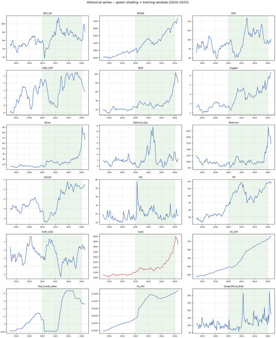
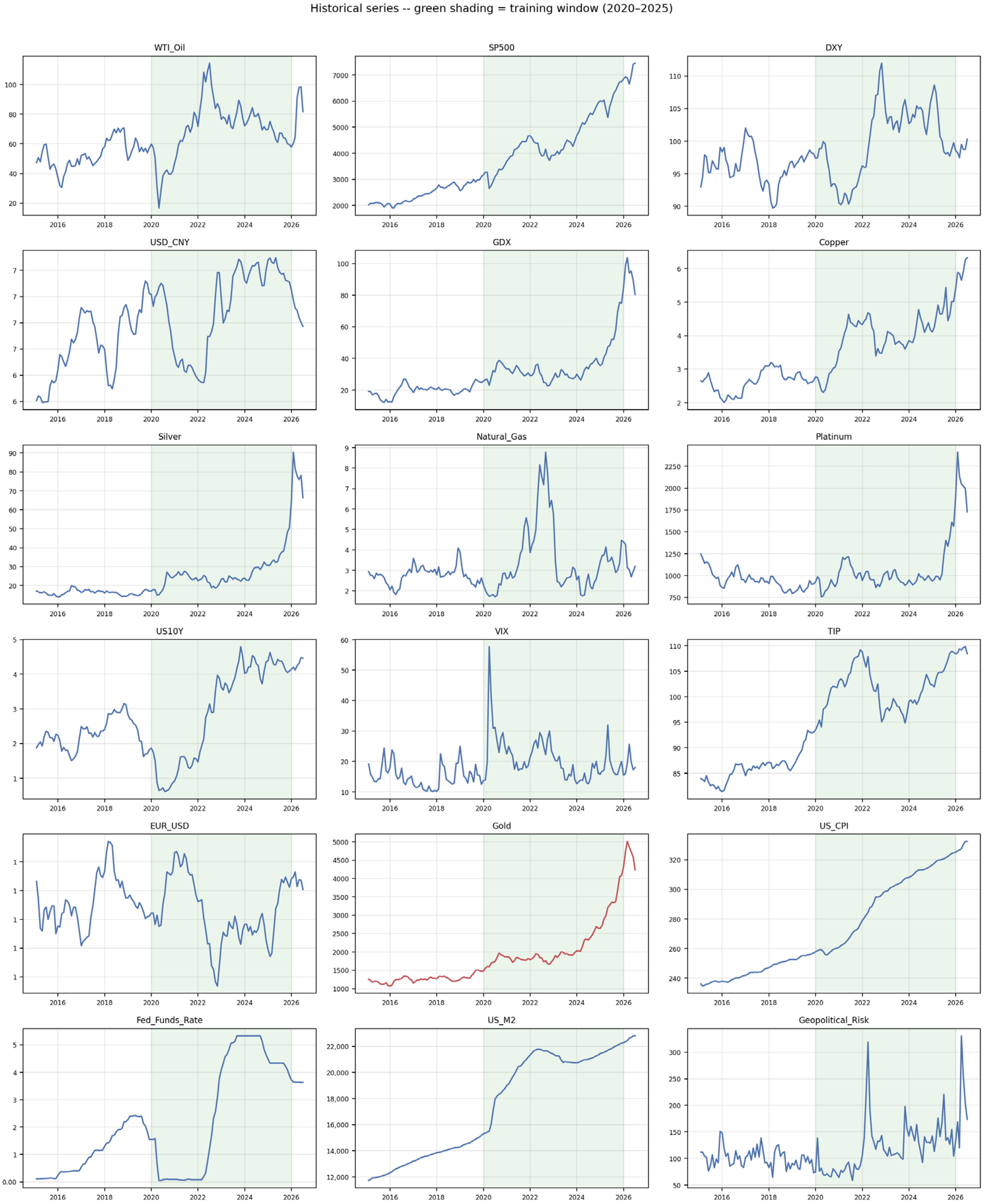
Figure 1 displays the historical monthly series for gold and all candidate predictors over the full sample.

Figure 1. Historical monthly series for gold and the seventeen candidate predictors (January 2015–June 2026); green shading marks the 2020–2025 training window.

An important methodological consideration is that monthly variables drawn from different sources may not be synchronously available at the time a forecast would actually be produced, even when they share the same calendar-month label. The thirteen original predictors are all derived from the same source (Yahoo Finance daily closing prices, averaged to a monthly frequency) and are therefore free of this concern by construction. This is not the case for the three FRED monetary series: the CPI and M2 are released with an approximate two-to-four-week publication lag relative to their reference month (for example, the CPI figure for March is not published until mid-April), whereas the effective federal funds rate is observable in near real time. To avoid look-ahead bias, the CPI and M2 series are shifted forward by one month before being merged into the panel, so that the value attributed to calendar month t is the value that would realistically have been public knowledge by the end of month t, rather than the reference-period value itself. The federal funds rate and the GPR index, both released with minimal lag relative to their reference period, are used without this adjustment.

3.2. Frequency and Sample Size

A monthly sampling frequency yields a comparatively small effective training sample (72 monthly observations under the 2020–2025 training window) relative to the number of model specifications considered. A daily or weekly frequency was considered but not adopted, for two reasons. First, three of the predictors—CPI, M2, and the GPR index—are natively available only at a monthly frequency (the GPR index is itself constructed as a monthly news-count measure); a daily reconstruction of the panel would require interpolating these series within each month, which would artificially manufacture daily variation that does not exist in the underlying data and would reintroduce the synchronization concern discussed in Section 3.1 rather than resolve it. Second, the sales-timing decision this model is designed to support (Section 5) is itself monthly, consistent with the typical commercialization cycle of ASM enterprises; a daily forecasting model would not directly map onto this decision frequency. As a partial response to the underlying concern about sample stability, Section 3.10 introduces a moving-block bootstrap of the cross-validation residuals and Section 4.7 introduces a fixed-window rolling-origin evaluation, both of which quantify the sensitivity of the reported accuracy metrics to the specific months included in each fold, without altering the underlying monthly frequency.

3.3. Stationarity Testing

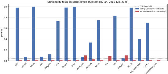
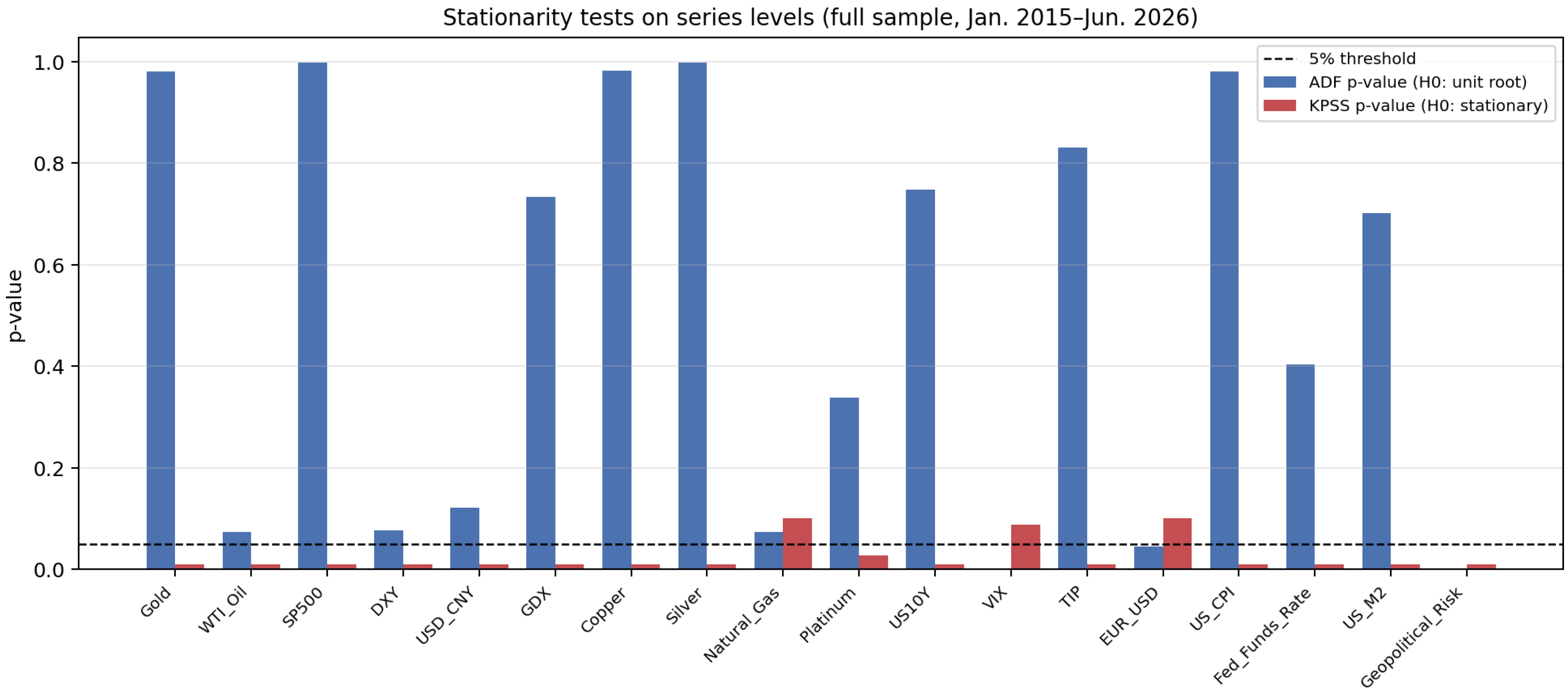
The Augmented Dickey–Fuller (ADF) test, with the null hypothesis of a unit root, and the Kwiatkowski–Phillips–Schmidt–Shin (KPSS) test, with the null hypothesis of stationarity, were applied to the levels of gold and all seventeen candidate predictors (thirteen original series plus GDX, GPR, CPI, the federal funds rate, and M2) over the full sample. Figure 2 reports the resulting p-values.

Figure 2. Stationarity tests on series levels (full sample, January 2015–June 2026). With the partial exception of the VIX and the EUR/USD exchange rate, all series fail to reject the null of a unit root (ADF) and reject the null of stationarity (KPSS), confirming that all series, including the newly added monetary and geopolitical indicators, are integrated of order one, I(1), in levels.

All subsequent modeling is therefore conducted on monthly log-returns (Section 3.4).

3.4. Log-Return Transformation and Johansen Cointegration

All series are transformed to monthly log-returns, r_t = ln(P_t) − ln(P_t−1), which are confirmed stationary by the ADF test for all seventeen candidates. A Johansen (1991) cointegration test is applied to the six-variable system (gold, S&P 500, the 10-year U.S. Treasury yield, silver, copper, and the U.S. Dollar Index) in levels. The trace statistic rejects the null hypothesis of zero, one, two, and three cointegrating vectors, but fails to reject the hypothesis of four, indicating four cointegrating relationships among gold and these five macro-financial variables. This result provides formal evidence of a long-run equilibrium structure linking gold to these variables; as discussed in Section 2.4, it is presented as complementary evidence contextualizing the short-run ML framework rather than as a prerequisite for it and motivates a VECM extension as future research (Section 6).

3.5. Predictor Screening: Granger Causality, Multicollinearity, and Feature Sets

To move from raw correlation toward a defensible predictive specification, each candidate predictor was tested for Granger causality toward gold log-returns (maxlag = 3), following the framework outlined in Section 2.4. The candidate set comprises seventeen series, combining the original thirteen macro-financial and commodity predictors with the GPR index, CPI, the federal funds rate, and M2 (Section 3.1). Table 1 reports the minimum p-value across lags 1–3 for each candidate.

Table 1. Granger causality tests (X → gold log-returns, maxlag = 3) for all seventeen candidate predictors, full sample.

Variable	Min. p-Value (Lags 1–3)	Granger-Causes Gold?	Role
S&P 500	0.0218	Yes	REDUCED/CONTROL
10-Year US Treasury Yield (US10Y)	0.0278	Yes	REDUCED/CONTROL
Copper	0.0846	No	REDUCED (theoretical)
VIX	0.0676	No	FULL only
M2 (new)	0.0602	No	FULL only
WTI Crude Oil	0.1479	No	REDUCED (theoretical)
CPI (new)	0.1504	No	FULL only
EUR/USD	0.2481	No	FULL only
Federal Funds Rate (new)	0.2133	No	FULL only
USD/CNY	0.3095	No	FULL only
DXY	0.3531	No	FULL only
TIP	0.4156	No	FULL only
Platinum	0.5271	No	REDUCED (theoretical)
Natural Gas	0.5362	No	REDUCED (theoretical)
Silver	0.5636	No	REDUCED (theoretical)
GPR (new)	0.5639	No	FULL only
GDX (reference)	0.8160	No	Excluded as primary predictor

None of the four monetary and geopolitical predictors (GPR, CPI, federal funds rate, M2) Granger-causes gold log-returns at the 5% level. This is a substantively informative null result rather than a modeling gap: it indicates that, once commodity co-movements and the existing S&P 500 and Treasury-Yield channels are accounted for, geopolitical risk and U.S. monetary conditions do not carry additional linear predictive content for one-month-ahead gold returns over this sample. Consistent with this finding, the REDUCED and CONTROL production feature sets (defined below) comprise only the commodity series and the two Granger-significant macro-financial variables; the four monetary and geopolitical variables enter only the FULL reference set.

Only the S&P 500 and the 10-year US Treasury yield Granger-cause gold log returns at the 5% level. Following the theoretical argument in Section 2.1, the five commodities series (WTI Oil, Copper, Silver, Natural Gas, and Platinum) are retained on theoretical grounds regardless of the Granger-test outcome, given their established role as co-moving real assets.

REDUCED (7 variables, excluding GDX): Copper, Natural Gas, WTI Crude Oil, Silver, Platinum, S&P 500, 10-Year US Treasury Yield.

CONTROL (8 variables): REDUCED plus a one-month-lagged GDX return, included as a non-contemporaneous control that avoids the endogeneity concern associated with GDX’s contemporaneous co-movement with gold.

FULL (17 variables, including contemporaneous GDX): All seventeen candidates, including the four new predictors, retained purely as a reference specification against which the production sets are compared.

FACTOR (2 variables): The five commodity aggregates plus a single principal-component factor (“PC1_Factor”) extracted, using loadings estimated only on the 2020–2025 training window to avoid look-ahead leakage, from the full seventeen-variable panel. This specification provides a low-dimensional diffusion-index alternative in the spirit of Stock and Watson (2002) and is evaluated alongside REDUCED, CONTROL, and FULL, though it is not eligible for selection as the production model (Section 3.7).

3.6. Multicollinearity (VIF)

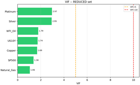
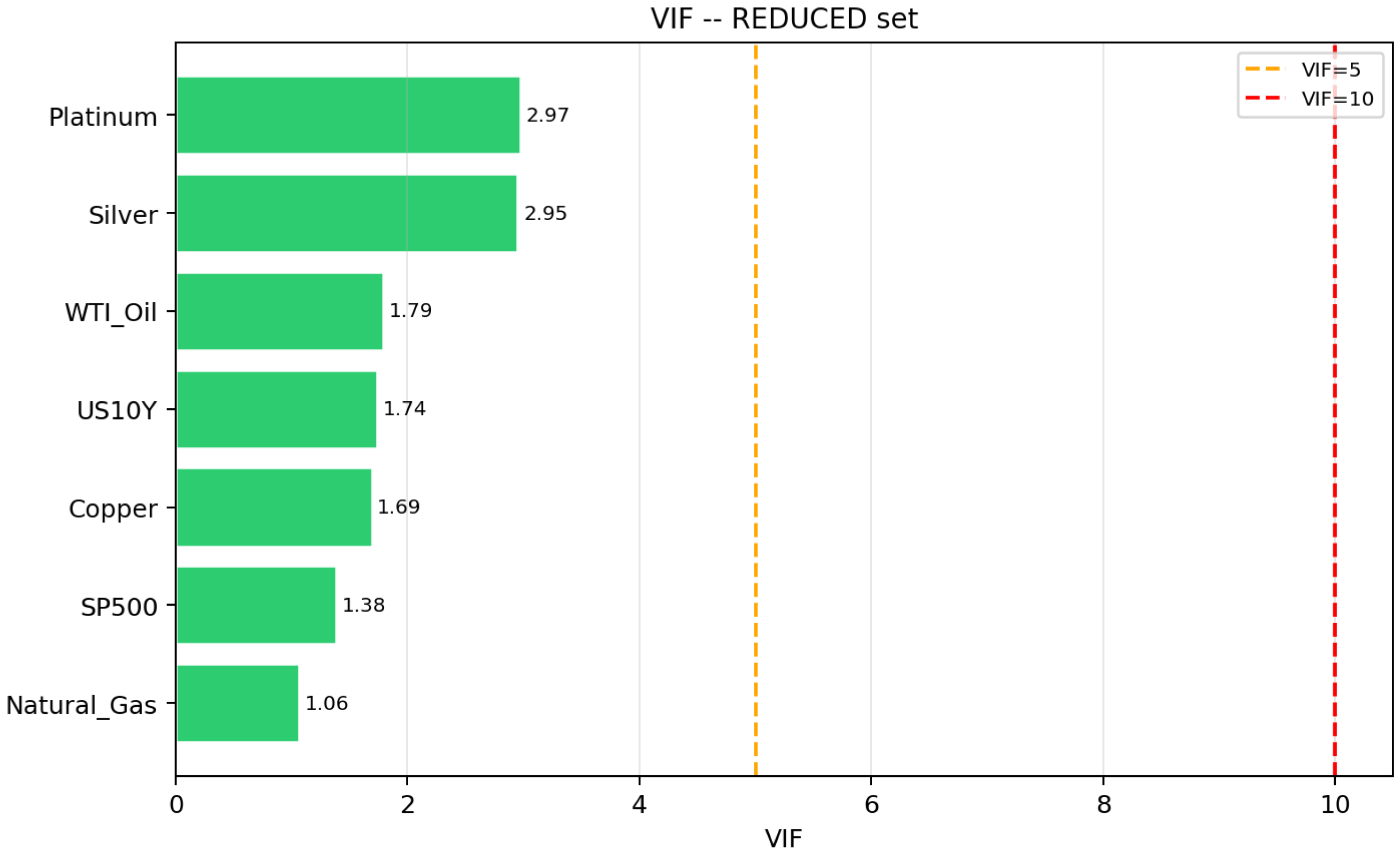
Before finalizing the REDUCED feature set, variance inflation factors (VIF) were computed over the 2020-2025 training window. All seven REDUCED-set variables show VIF values below 3.0 (Table 2, Figure 3), indicating no material multicollinearity concern.

Table 2. Variance inflation factors for the REDUCED feature set, training window 2020–2025.

Variable	VIF	Assessment
Platinum	2.97	OK
Silver	2.95	OK
WTI Crude Oil	1.79	OK
10-Year US Treasury Yield	1.74	OK
Copper	1.69	OK
S&P 500	1.38	OK
Natural Gas	1.06	OK

Figure 3. Variance inflation factors, REDUCED feature set.

3.7. Model Specification and Hyperparameter Selection

Eight ML algorithms (Linear Regression, Ridge, Random Forest, XGBoost, LightGBM, Support Vector Regression with an RBF kernel, Elastic Net, and Bayesian Ridge) were trained and evaluated on each of the four feature sets (REDUCED, CONTROL, FULL, FACTOR), yielding thirty-two set-by-model combinations. Hyperparameters for each tunable model are selected via a grid search (scikit-learn GridSearchCV) conducted over a deliberately bounded parameter grid, using the same five-fold expanding TimeSeriesSplit cross-validation described in Section 3.8, so that no test-period information enters the selection. The search is a single-level (non-nested) procedure: a fully nested grid search, with an inner cross-validation loop within each outer fold, was considered and not adopted, because it would further shrink the already-limited training subsample available to each inner fold (as few as 12–15 monthly observations), a design choice that is disclosed here rather than presented as a limitation to be discovered later. The final production model uses the hyperparameters selected by this procedure (α = 0.5 for the selected Ridge specification; see Section 4.1). Linear Regression and Bayesian Ridge, whose hyperparameters are either absent or estimated internally via evidence maximization, are used without an external grid.

Two econometric benchmarks were evaluated explicitly. An ARIMA(2,1,2) model was fitted to the gold price level series; it produced a test-period MAPE an order of magnitude worse than any ML specification and exhibited a divergent, unbounded trajectory when projected beyond the test horizon. Rather than silently omitting this benchmark, it is reported here explicitly and excluded from production forecasting on the documented grounds of instability. A GARCH(1,1) model was fitted to the gold log-return series and is retained solely as a volatility diagnostic (Section 4.7), not as a level-forecasting benchmark, consistent with its role in the literature (Bollerslev, 1986).

Long short-term memory (LSTM) and other deep learning architectures, and state-space or Markov-switching regime models, while prominent in the recent literature, were not implemented in this study. This is a deliberate methodological decision: the training sample available under the strict 2020–2025 temporal partition comprises only 72 monthly observations, which is insufficient to fit a Markov-switching model or a deep recurrent architecture without a material risk of non-convergence or severe overfitting. This limitation is stated transparently as a boundary condition of the present study and is revisited as a direction for future research in Section 6.

3.8. Temporal Validation: Train/Test Partition and Sensitivity Window

The training period spans January 2020–December 2025 (72 monthly observations), and the official test period spans January–June 2026 (the most recent complete data available at the time of analysis). No observation from the test period is used, directly or indirectly, in model fitting, hyperparameter selection, or feature-set construction. Within the training period, model selection across the thirty-two set-by-model combinations was conducted using an expanding-window TimeSeriesSplit cross-validation with five folds and a one-period gap between each training fold and its corresponding validation fold, eliminating the risk of look-ahead bias inherent in random partitioning of time-ordered data (Tsay, 2010).

To assess whether the ranking of model specifications is sensitive to the small number of official test-period observations, a second, extended sensitivity partition was constructed by moving the train/test cutoff backward to July 2025, yielding a ten-month test window (August 2025–May 2026). All thirty-two set-by-model combinations were re-estimated and re-evaluated on this extended window; results are reported alongside the official-window results in Section 4.1 and Section 4.2.

3.9. Naive Benchmarks and Forecast-Comparison Tests

The production model is compared against three naive forecasting rules: a random-walk forecast (predicted return equal to zero), the historical mean return of the training sample, and simple exponential smoothing applied to the gold price level (Campbell & Thompson, 2008, establish that surpassing the historical average out-of-sample is a demanding benchmark for any predictive model; Rapach et al., 2010, report a similar pattern for equity-premium forecasts combined across models). Four formal statistical tests are then applied to the resulting forecast errors. The Diebold–Mariano test (Diebold & Mariano, 1995) compares the production model against each of the three non-nested naive benchmarks. Because the REDUCED, CONTROL, and FULL feature sets are nested by construction (CONTROL nests REDUCED; FULL nests CONTROL), a standard Diebold–Mariano comparison among them would be biased toward over-rejection of the null of equal accuracy (West, 1996); the Clark–West correction (Clark & West, 2007, building on West, 1996) is used instead for these nested comparisons. A forecast-encompassing test (Harvey et al., 1998) evaluates whether the production model’s forecast errors are explained, in part, by the naive benchmarks’ errors, which would indicate that the benchmark carries information the production model does not capture. Finally, a Model Confidence Set (Hansen et al., 2011) is constructed over the squared forecast-error loss of the production model and the three benchmarks, identifying, at a chosen confidence level, the subset of models that cannot be statistically distinguished from the best performer. All four tests are reported together with an explicit caveat: with a test window of five to ten monthly observations, each test has materially reduced statistical power, and a failure to reject a null of equal accuracy may simply reflect this limited power rather than genuine equivalence between models (Section 4.5).

3.10. Monte Carlo Simulation and Distributional Robustness

The final model is retrained on the full available history and used to generate a dual-horizon forecast (tactical, through December 2026; strategic, through December 2027) via Monte Carlo simulation with 100,000 iterations. Predictor shocks are drawn jointly from a multivariate normal distribution parameterized by the historical mean and covariance of the training-window log-returns (primary scenario: zero drift; sensitivity scenario: historical drift); model-error shocks are drawn by bootstrap resampling from the pooled out-of-sample cross-validation residuals.

The assumption of joint normality for predictor shocks is not assumed without verification. Table 3 reports skewness and excess kurtosis for each of the market-return variables entering the Monte Carlo simulation. Several series, most notably the S&P 500 and the 10-year Treasury yield, exhibit material excess kurtosis and negative skewness, both stylized facts of financial returns documented extensively elsewhere (Cont, 2001) and inconsistent with strict multivariate normality. To quantify the practical consequence of this departure, a third simulation scenario draws predictor shocks from a multivariate Student-t distribution (5 degrees of freedom, scaled to match the historical covariance) rather than a multivariate normal, holding all other elements of the simulation fixed. The resulting uncertainty band is compared to the primary normal-shock scenario in Section 4.8 and Figure 4.

Table 3. Skewness and excess kurtosis of the log-return shocks used in the Monte Carlo simulation, training window 2020–2026.

Variable	Skewness	Excess Kurtosis	Jarque–Bera p-Value
S&P 500	−2.31	9.61	<0.001
10-Year US Treasury Yield	−1.69	8.26	<0.001
WTI Crude Oil	−0.68	7.54	<0.001
Silver	0.92	2.67	<0.001
Copper	−1.06	2.36	<0.001
Natural Gas	−0.74	1.20	0.003
Platinum	0.17	1.73	0.006
GDX (control)	0.08	−0.51	0.627

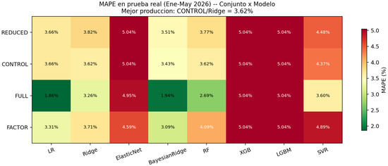
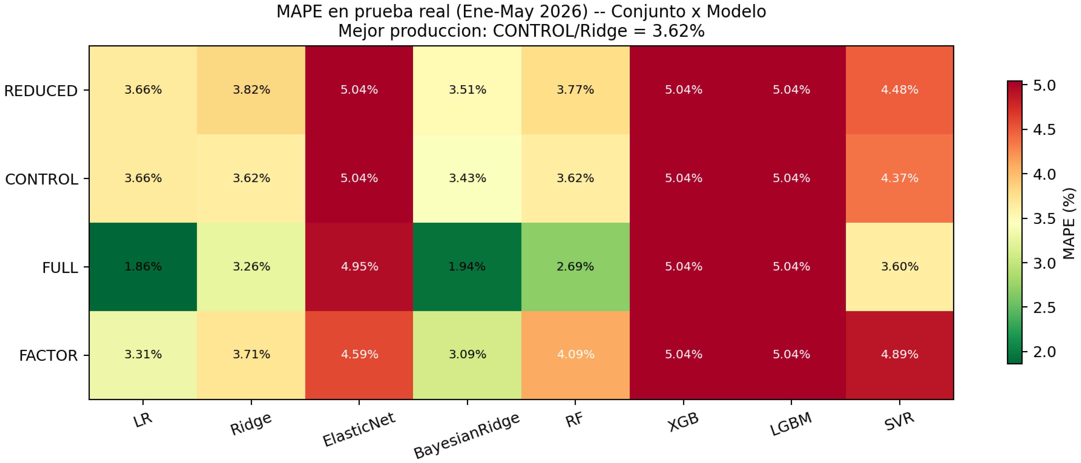
Figure 4. Out-of-sample test MAPE (official window) by feature set and model.

3.11. Structural Breaks and Long-Memory Diagnostics

Beyond volatility clustering (addressed via the GARCH diagnostic, Section 4.7) and heavy tails (Section 3.10), two further stylized facts of commodity and financial markets, structural breaks and long-memory dependence, are examined explicitly. A Chow test compares the fit of an auxiliary OLS regression of gold returns on the REDUCED feature set before and after January 2024, a candidate break date corresponding to the documented onset of the elevated gold price regime discussed in Section 1 (BCRP, 2025; Rumbo Minero, 2024). This auxiliary regression is used exclusively for this diagnostic and does not replace the production ML model used for forecasting. A Hurst exponent, estimated via a variance-scaling regression on the gold log-return series, assesses the presence of long-memory dependence.

The Chow test rejects the null of coefficient stability at the break date (F = 2.86, p = 0.006), indicating that the relationship between gold returns and the REDUCED predictors is not constant across the full sample, consistent with the documented regime shift toward structurally higher and more volatile gold prices from 2024 onward. The estimated Hurst exponent for monthly gold returns is close to zero and, in this application, falls outside the canonical (0,1) range for a well-behaved long-memory process; we interpret this as reflecting the limited precision of a simple variance-scaling estimator applied to a monthly series of moderate length (n = 137) rather than as reliable evidence of anti-persistence, and recommend a more robust long-memory estimator applied to higher-frequency data as a direction for future work (Section 6).

3.12. Interpretability: SHAP Values and Partial Dependence

Beyond the Random Forest’s built-in feature-importance measure (based on impurity reduction), which quantifies overall predictor relevance but not the direction or functional form of each predictor’s effect, SHAP (SHapley Additive exPlanations) values are computed via a tree or linear explainer matched to the production model’s algorithm family, together with partial dependence plots for the three most influential predictors identified by the SHAP analysis (Section 4.4).

4. Results

4.1. Model Development, Selection, and Validation

Production-model eligibility is fixed by design, prior to inspecting any test-set result: only the REDUCED and CONTROL feature sets, combined with the six algorithms used throughout the study’s original design (Linear Regression, Ridge, Random Forest, XGBoost, LightGBM, and SVR; Section 3.7), may be selected as the production model. FULL, FACTOR, Elastic Net, and Bayesian Ridge are evaluated and reported in every table and figure below as transparent benchmarks, but are not eligible for selection, a rule stated here explicitly and prominently to avoid any impression that model selection was adjusted post hoc once results were known.

Table 4 reports cross-validation and out-of-sample test performance for the production-eligible combinations (REDUCED and CONTROL, across the six original algorithms) together with the reference-only combinations (FULL, FACTOR, and the two new model families, Elastic Net and Bayesian Ridge, shown for completeness but not eligible for production selection; see rationale below). Figure 4 visualizes the full 4 × 8 comparison grid.

Table 4. Cross-validation and out-of-sample test performance, official and sensitivity partitions (* = selected production model). Full thirty-two-combination results are provided in the Supplementary Comparison File.

Set	Model	CV MAPE	Test MAPE (Official, n = 6)	Test MAPE (Sensitivity, n = 10)
REDUCED	LR	1.87%	3.66%	3.22%
REDUCED	Ridge	2.30%	3.82%	3.24%
REDUCED	RF	2.01%	3.77%	3.40%
REDUCED	SVR	2.05%	4.48%	3.86%
CONTROL	LR	1.85%	3.66%	3.24%
CONTROL	Ridge *	2.29%	3.62%	3.15%
CONTROL	RF	2.02%	3.62%	3.47%
CONTROL	SVR	2.09%	4.37%	4.05%
FULL (reference)	LR	1.81%	1.86%	1.96%
FULL (reference)	BayesianRidge	1.44%	1.94%	1.94%
FACTOR (reference)	BayesianRidge	2.04%	3.09%	2.86%
REDUCED/CONTROL (reference)	ElasticNet	2.79%	5.04%	4.47%

Consistent with the eligibility rule stated above, the best-performing combination overall, FULL/LR (test MAPE 1.86%), and FACTOR/Bayesian Ridge (test MAPE 3.09%), which outperforms every REDUCED/CONTROL combination except CONTROL/Ridge, are both reported in Table 4 but excluded from selection: FULL relies on contemporaneous GDX, which does not Granger-cause gold returns (Table 1), and the wider thirty-two-combination grid increases the risk that a nominally “best” result in a short test window reflects sampling variation rather than genuine improvement.

Within this restricted grid, CONTROL/Ridge achieves the lowest official-window test MAPE (3.62%), with a cross-validation MAPE of 2.29% (±0.35%) and the hyperparameter α = 0.5 selected by the grid search described in Section 3.7. CONTROL/Ridge is therefore selected as the production model for all subsequent analysis.

4.2. Sensitivity to the Test-Window Length

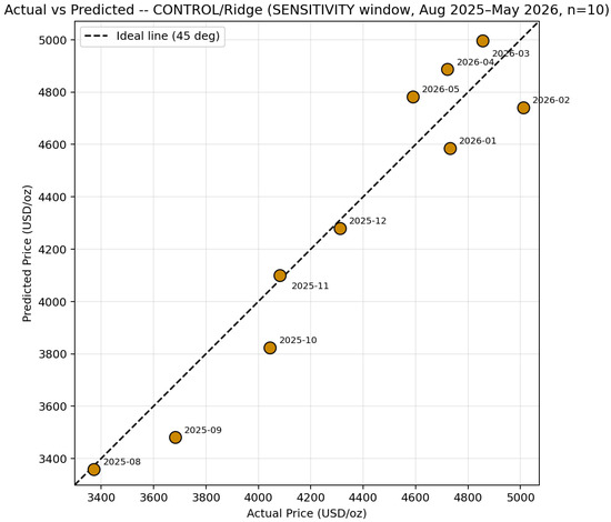
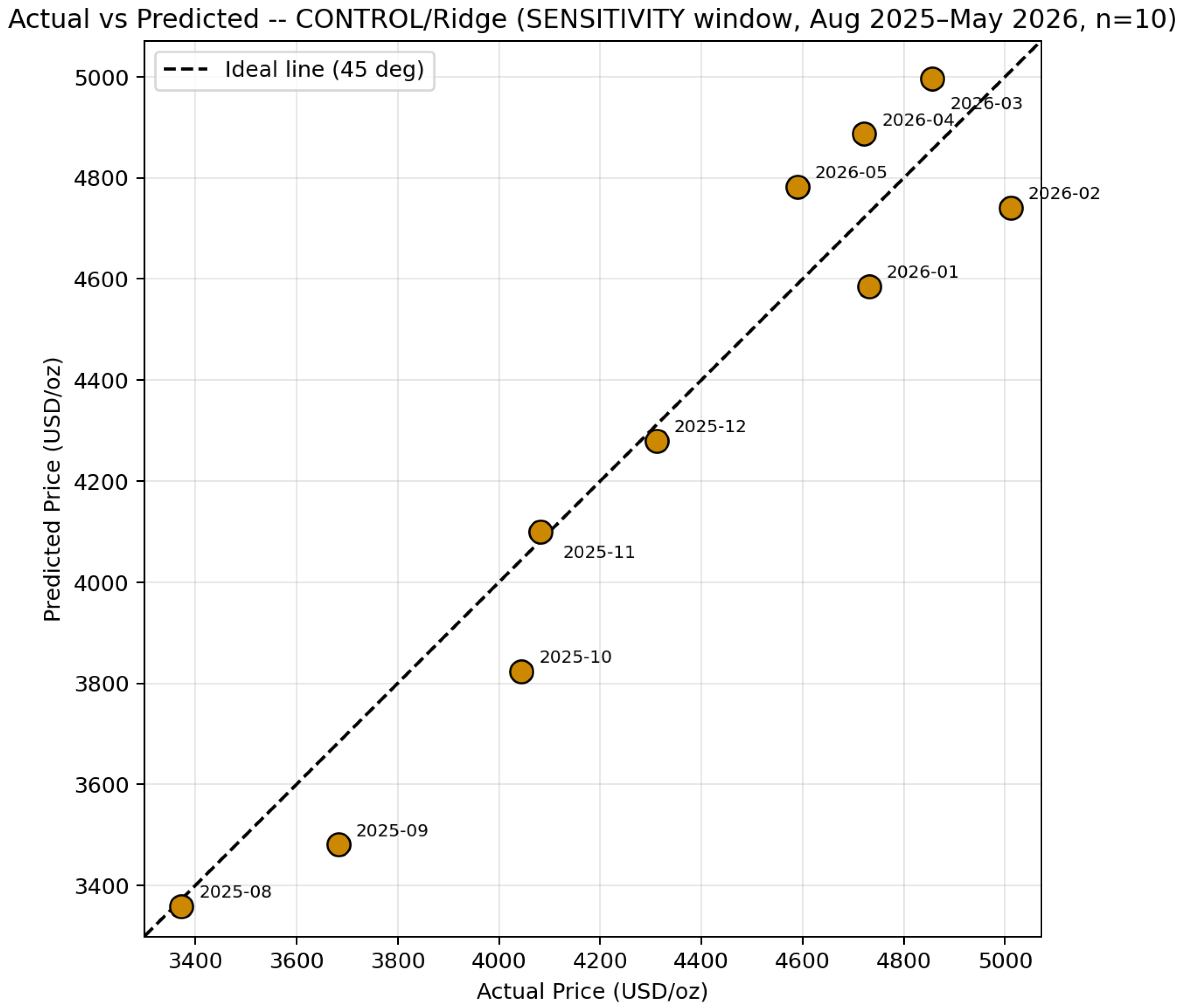
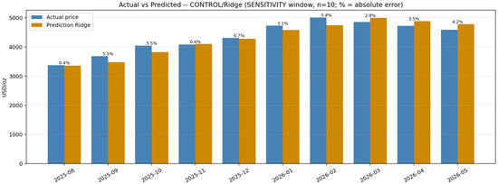
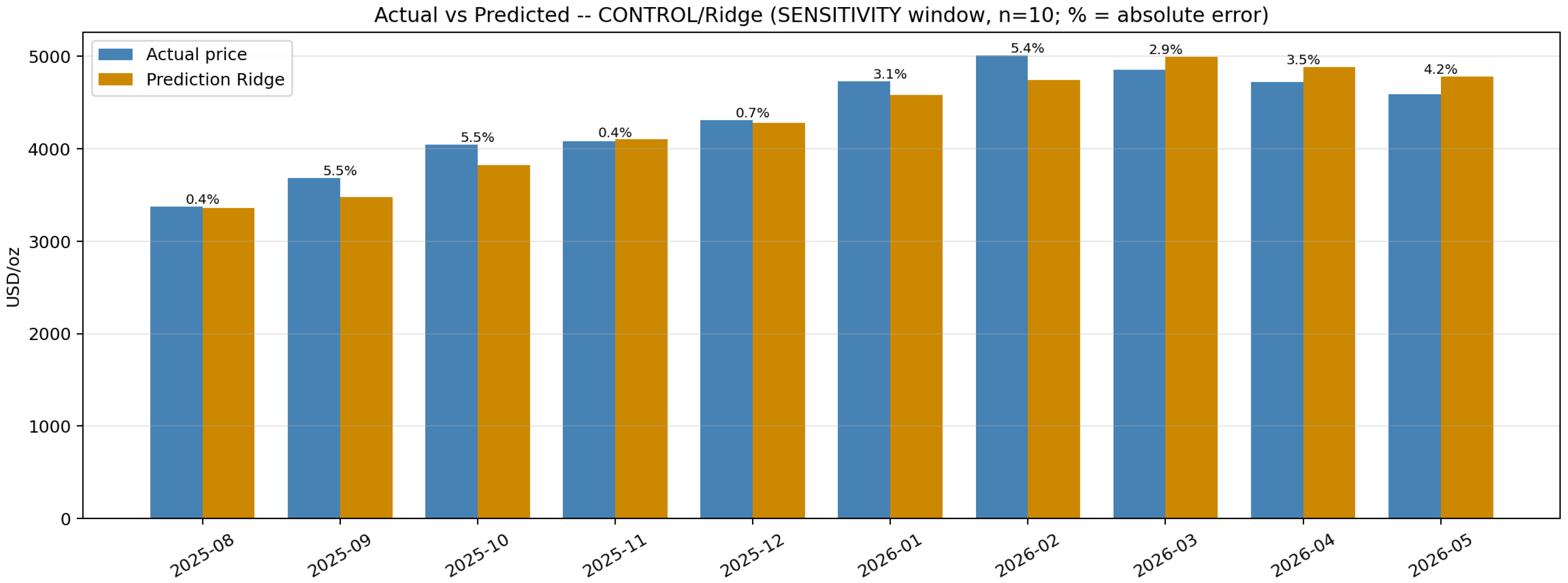
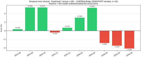
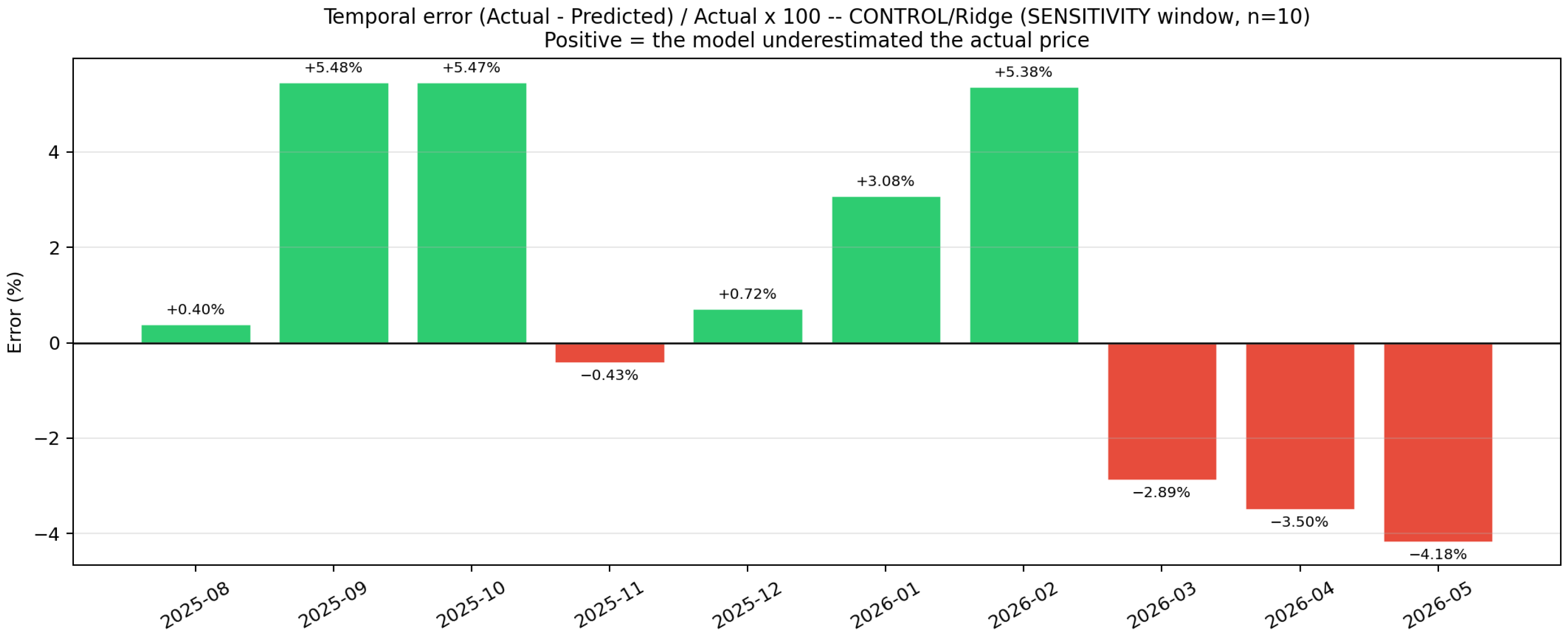
Under the extended, ten-month sensitivity window (August 2025–May 2026), CONTROL/Ridge remains the best-performing combination within the restricted production grid, with a test MAPE of 3.15%, closely tracking (and marginally improving on) the official-window estimate of 3.62%. Figure 5 plots actual against predicted prices for this extended window, and Figure 6 presents the same comparison as paired bars; both show predictions closely tracking the elevated-price trajectory observed from August 2025 onward, without a systematic directional bias toward over- or under-prediction. Figure 7 presents the corresponding temporal error pattern, which remains bounded within a similar range to the official window (no monthly error exceeding approximately ±7%) and shows no evidence of drift or a widening trend over the ten-month period. Taken together, these three figures provide reassurance that the January–May 2026 result is not an artifact of an unusually favorable five-month sample, though the same caveat regarding limited statistical power (Section 3.9) applies to any comparison based on a ten-month window.

Figure 5. Actual vs. predicted gold price, CONTROL/Ridge, extended sensitivity window (August 2025–May 2026, n = 10).

Figure 6. Actual vs. predicted gold price (bar comparison), extended sensitivity window.

Figure 7. Temporal error pattern, extended sensitivity window.

4.3. Naive Benchmarks and Forecast-Comparison Tests Results

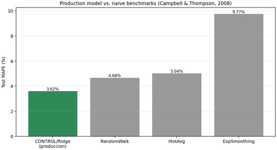
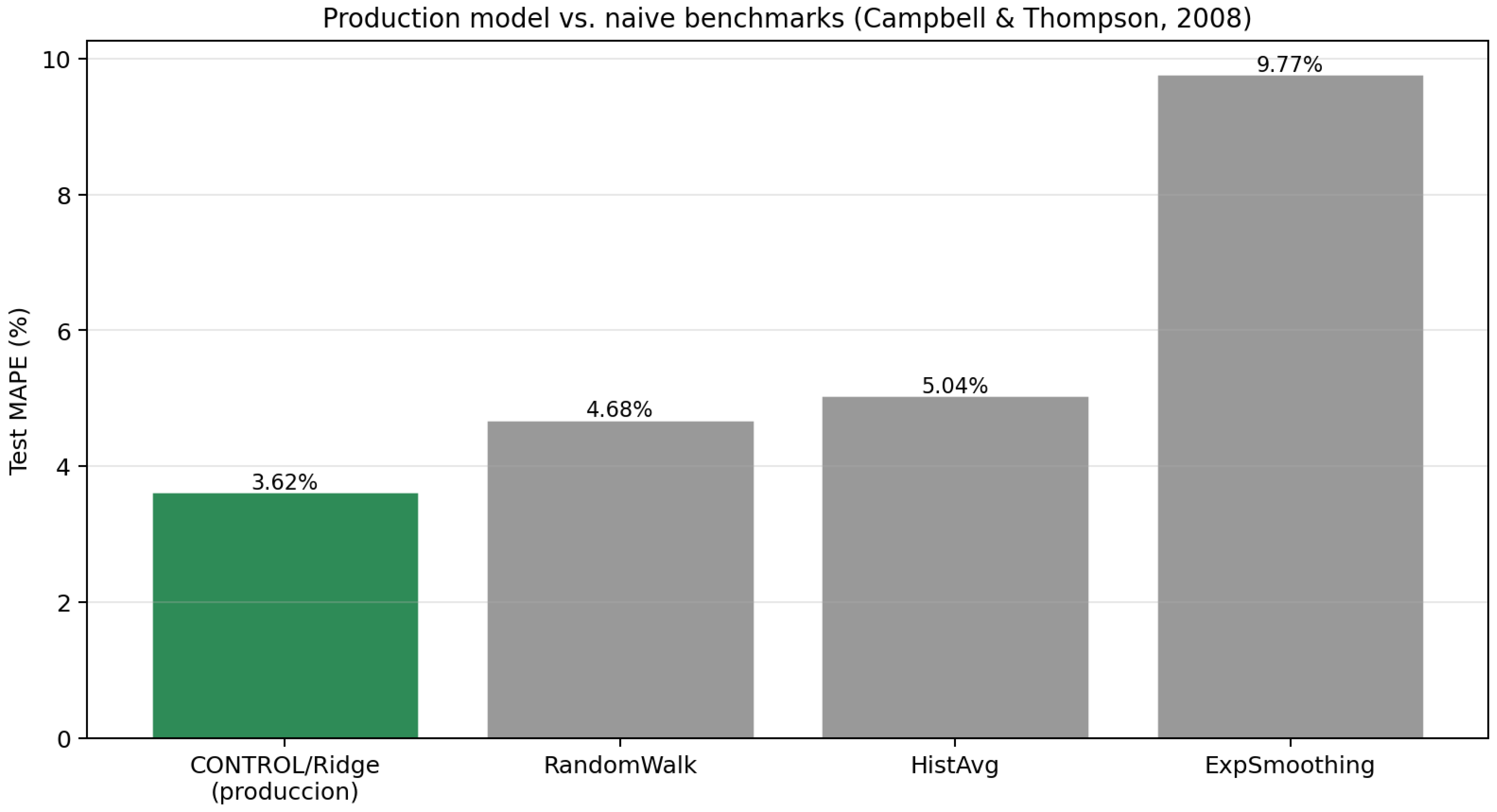
Table 5 and Figure 8 compare the production model against the three naive benchmarks described in Section 3.9. CONTROL/Ridge outperforms all three in point accuracy, though by a narrower margin against the random walk (4.68% MAPE) and the historical mean (5.04% MAPE) than against exponential smoothing (9.77% MAPE), which performs poorly on this short, elevated-price-regime test window.

Table 5. Production model vs. naive benchmarks, official test window.

Model	MAE (USD/oz)	RMSE (USD/oz)	Test MAPE
CONTROL/Ridge (production)	173.71	182.68	3.62%
Random walk	224.26	250.69	4.68%
Historical mean	240.85	247.73	5.04%
Simple exponential smoothing	470.86	491.89	9.77%

Figure 8. Production model vs. naive benchmarks (Campbell & Thompson, 2008).

Table 6 reports the formal comparison tests described in Section 3.9. The Clark–West test finds a statistically significant improvement of the nested FULL specification over REDUCED (p = 0.022) but only marginal evidence for CONTROL over REDUCED (p = 0.039, significant at 5% but based on very few effective degrees of freedom). Diebold–Mariano tests find the production model significantly more accurate than exponential smoothing (p < 0.001) but do not reject equal accuracy against the random walk or the historical mean (p = 0.34 and p = 0.19, respectively). The forecast-encompassing tests do not reject the null that the production model encompasses any of the three benchmarks. The Model Confidence Set (α = 0.25) retains the random walk and the production model, excluding the historical mean and exponential smoothing. Consistent with the power caveat stated in Section 3.9, these results should be read as showing that the production model is never significantly worse than the naive benchmarks and is significantly better than one of them (simple exponential smoothing), while the comparison against the random walk and the historical mean remains statistically inconclusive given the small test sample, a limitation stated openly rather than obscured.

Table 6. Formal forecast-comparison tests. All tests computed on a test window of n = 6 (official); interpret with caution given limited statistical power.

Test	Comparison	Statistic	p-Value
Clark–West	REDUCED vs. CONTROL	1.76	0.039
Clark–West	REDUCED vs. FULL	2.01	0.022
Diebold–Mariano	Production vs. Random Walk	−0.96	0.337
Diebold–Mariano	Production vs. Historical Mean	−1.30	0.194
Diebold–Mariano	Production vs. Exp. Smoothing	−3.59	<0.001
Forecast Encompassing	Production vs. Random Walk	−0.46	0.677
Forecast Encompassing	Production vs. Historical Mean	−0.47	0.670
Forecast Encompassing	Production vs. Exp. Smoothing	1.23	0.306
Model Confidence Set (α = 0.25)	Included: Random Walk, Ridge	—	—

4.4. Production Model Fit over the Historical and Test Periods

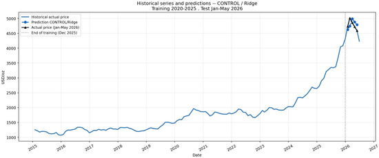
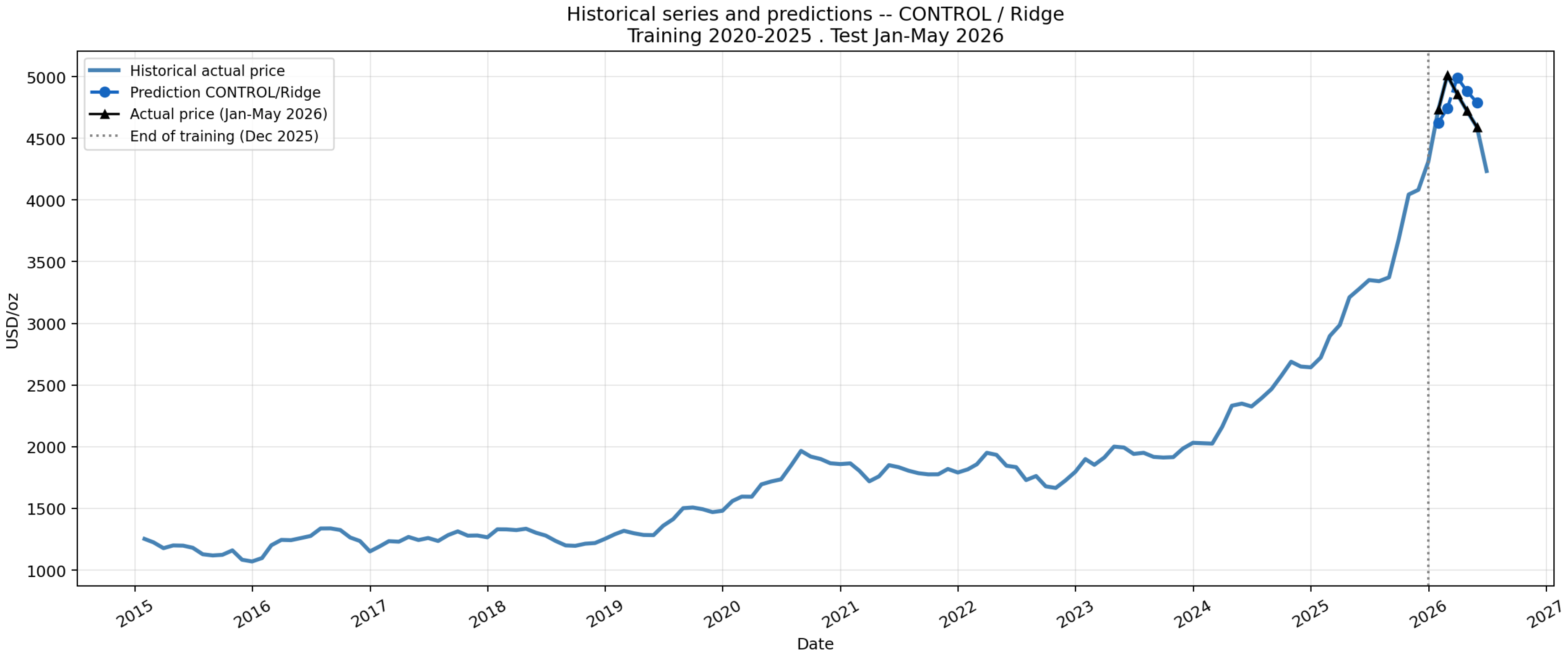
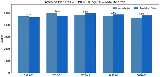
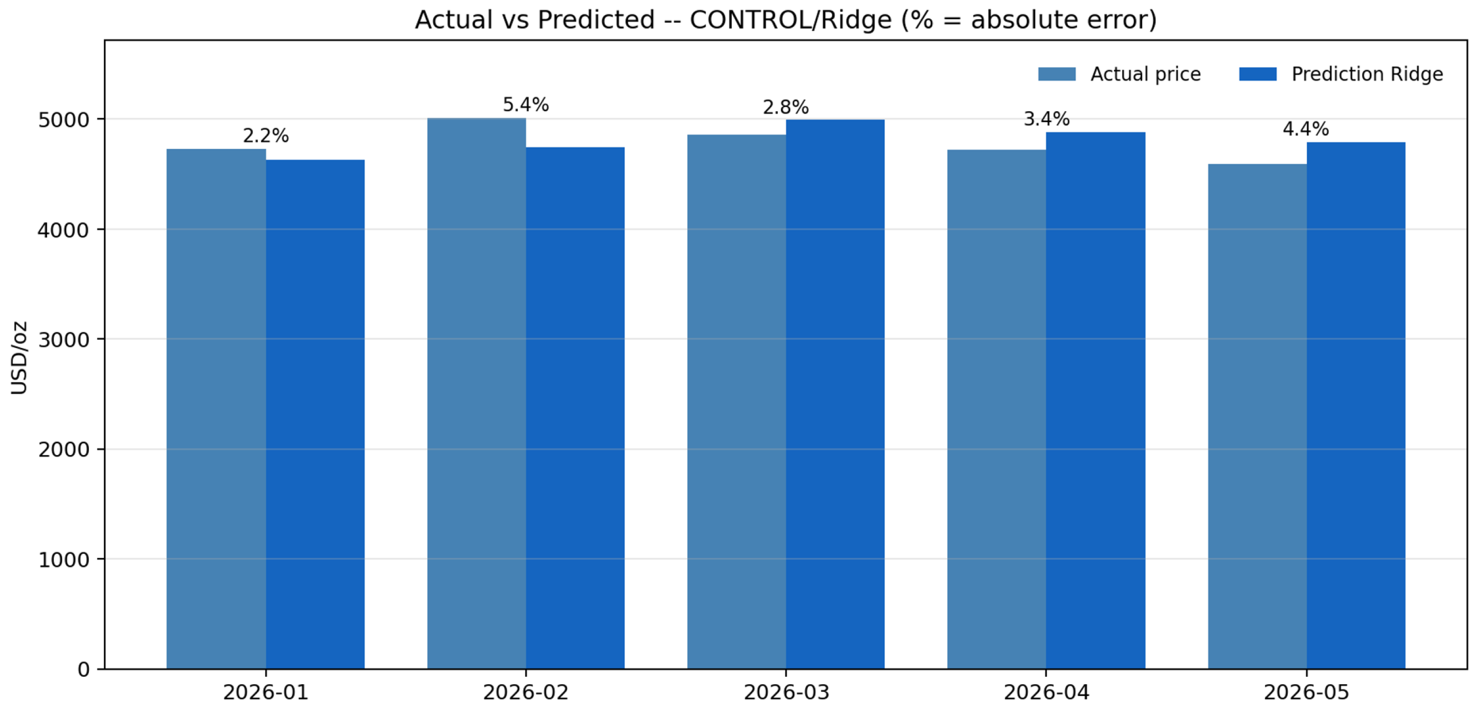
Figure 9 plots the historical gold price series together with the production model’s test-period predictions, and Figure 10 presents the same comparison as paired bars for direct visual inspection of each month’s absolute error.

Figure 9. Historical gold price series (January 2015–June 2026) with CONTROL/Ridge predictions for the official test window.

Figure 10. Actual versus predicted gold prices, CONTROL/Ridge, official test window (January–June 2026).

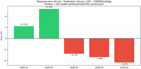
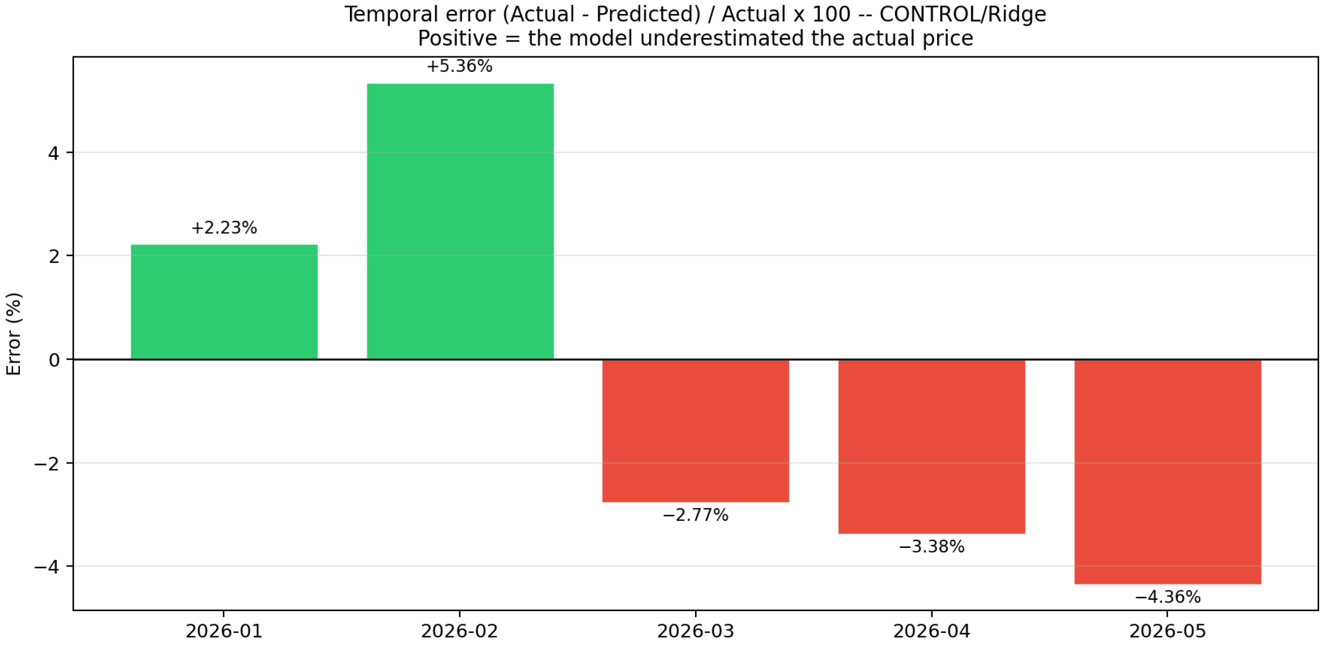
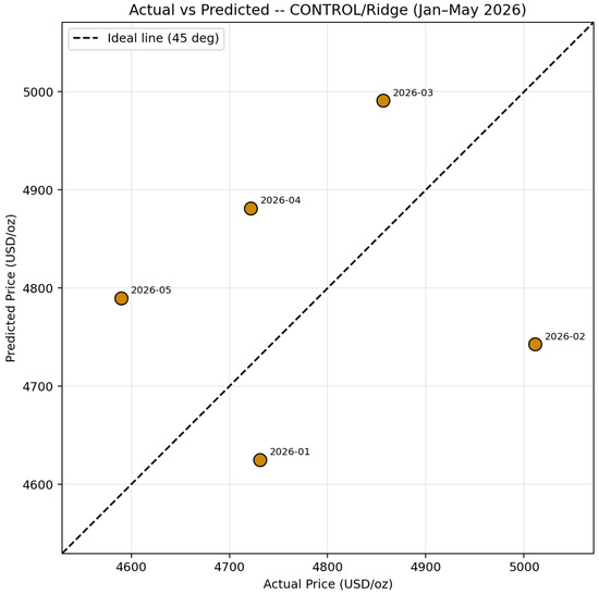
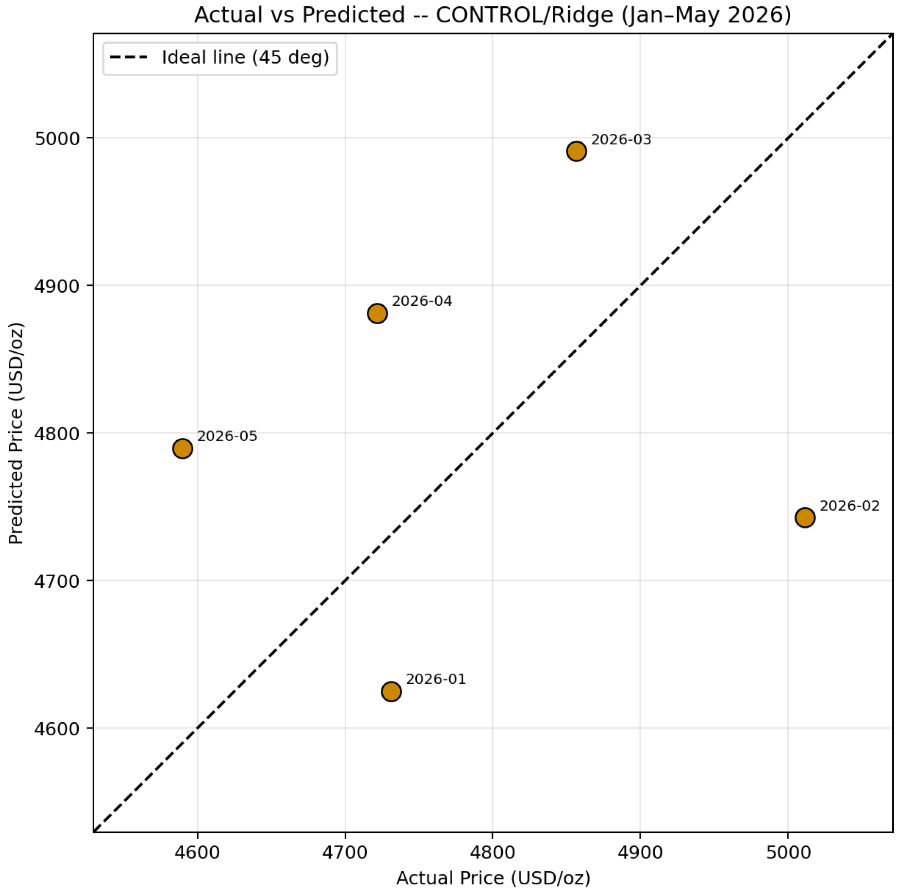
Figure 11 presents the temporal pattern of signed error (actual minus predicted, as a percentage of the actual price), and Figure 12 presents the actual-vs-predicted values as a scatter plot against the 45-degree line of perfect prediction.

Figure 11. Temporal error pattern, CONTROL/Ridge, official test window.

Figure 12. Actual vs Predicted-CONTROL/Ridge (January–May 2026).

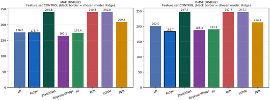
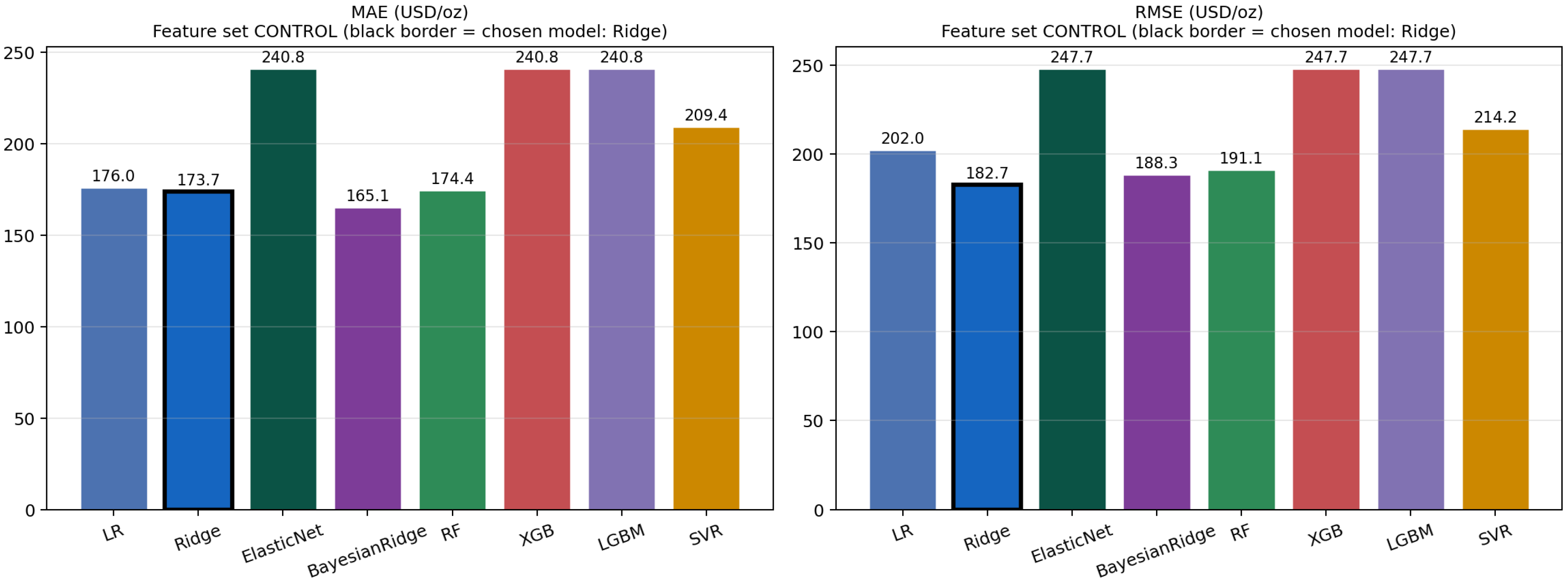
Figure 13 reports MAE and RMSE across all models within the production CONTROL feature set, confirming that Ridge achieves the lowest error of the six original algorithms once hyperparameters are tuned (Section 3.7).

Figure 13. MAE and RMSE by model within the CONTROL feature set, official test window.

4.5. Residual Diagnostics and Interpretability

Residual diagnostics for CONTROL/Ridge show a Durbin-Watson statistic of 1.15, a Ljung–Box p-value of 0.29 (no significant residual autocorrelation), a Jarque–Bera p-value of 0.72, and a Shapiro–Wilk p-value of 0.23 (both failing to reject normality of the test-period residuals).

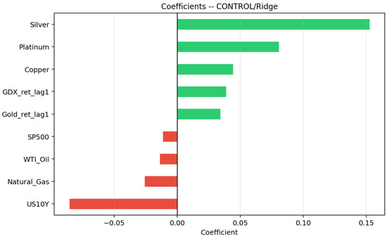
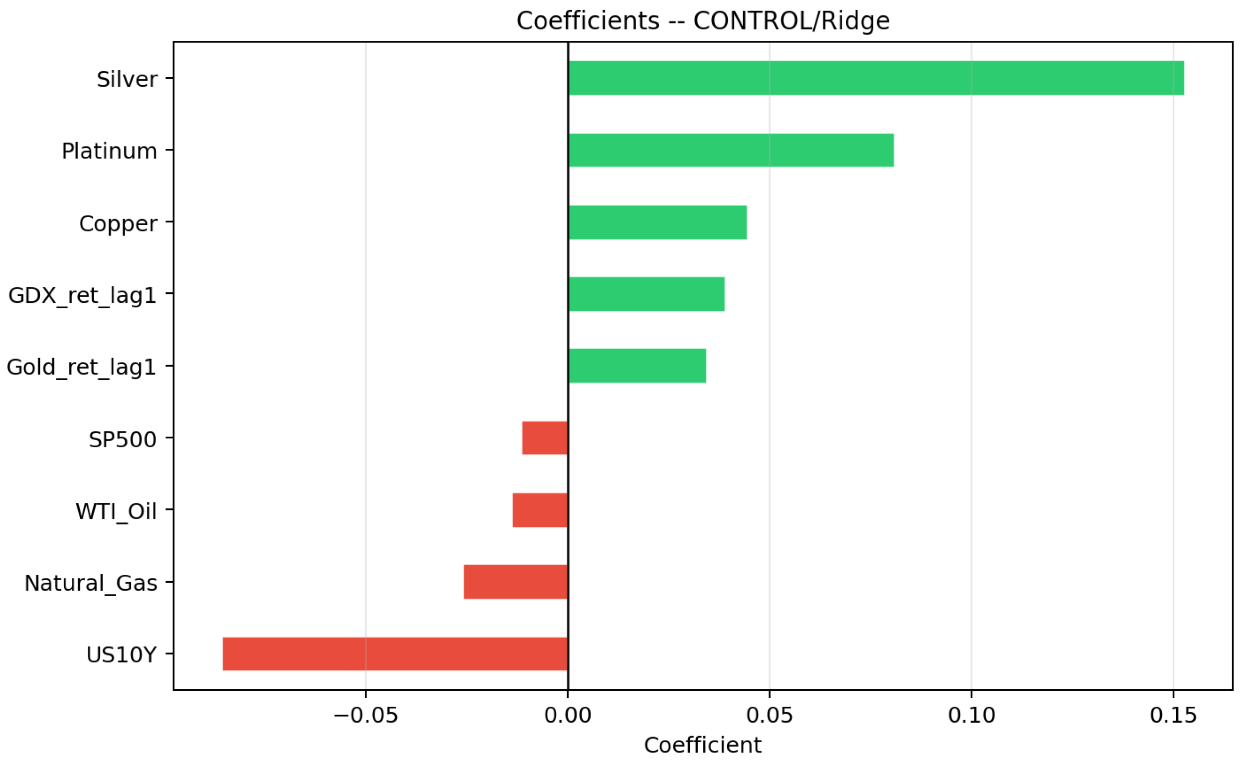
Figure 14 reports the standardized coefficients of the retrained production model, consistent with the Ridge specification selected via the hyperparameter search described in Section 3.7; Section 4.6 quantifies each predictor’s relative influence.

Figure 14. Standardized coefficients, CONTROL/Ridge production model.

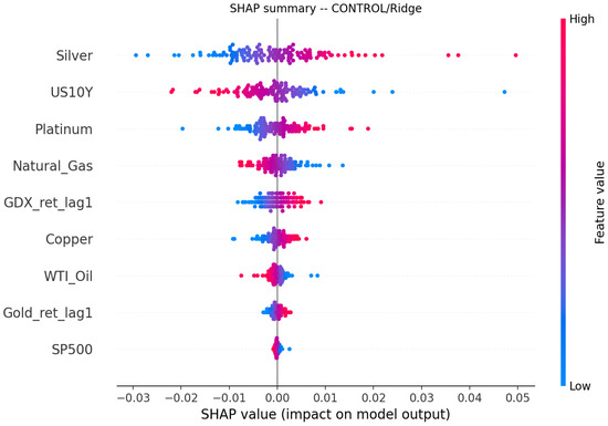
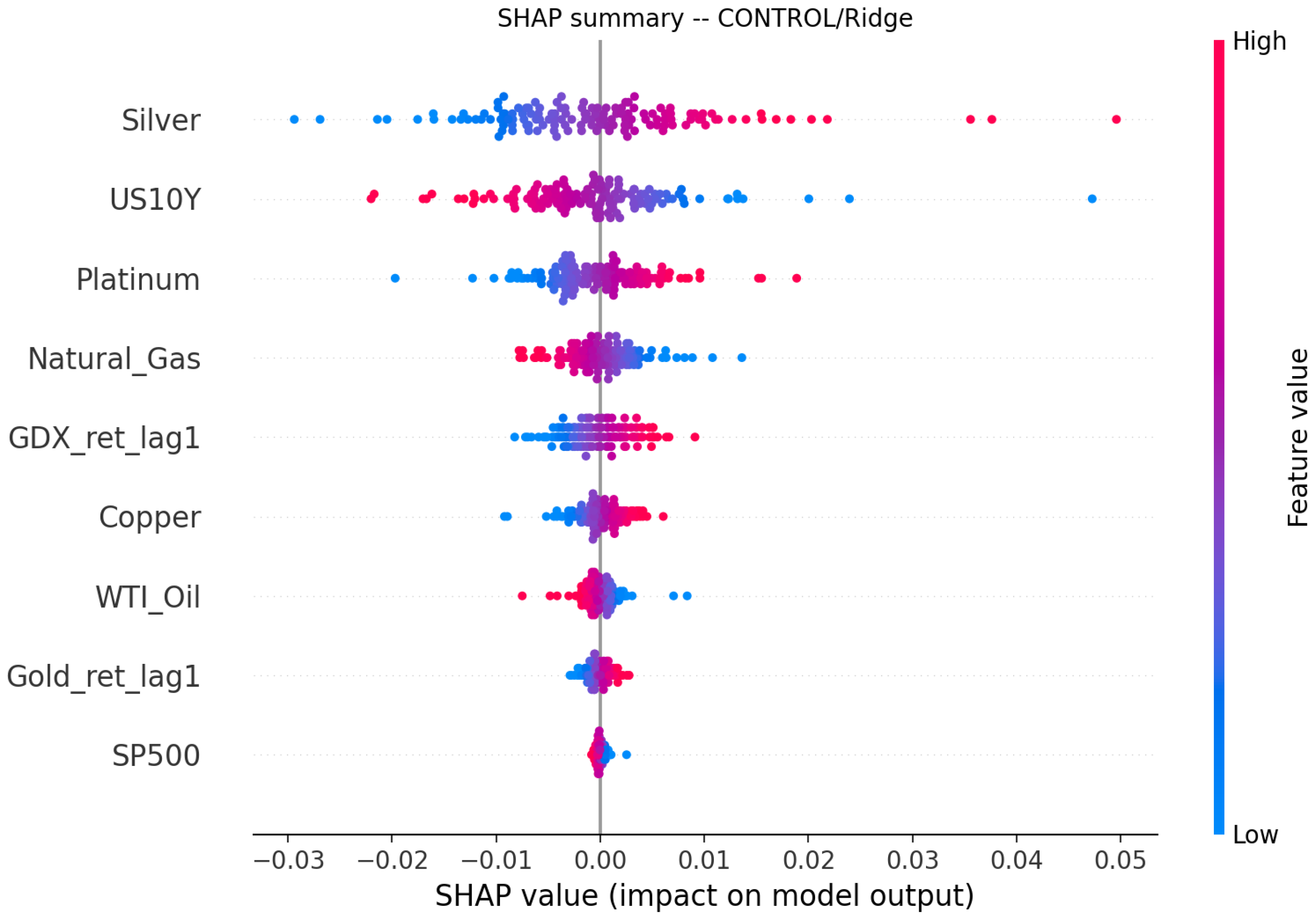
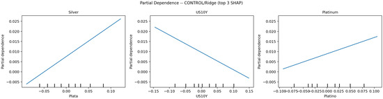
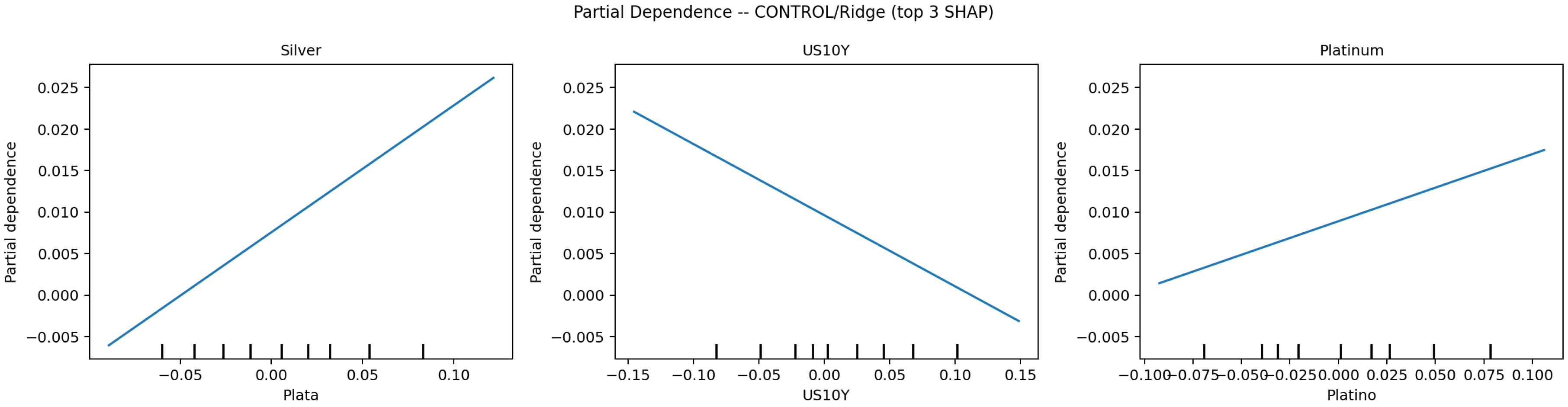
Figure 15 presents SHAP values for the production model’s linear coefficients, and Figure 16 presents partial dependence plots for the three predictors with the largest mean absolute SHAP value. Consistent with the coefficients reported above, the 10-year Treasury yield and the S&P 500 are the two most influential predictors, with the expected signs (a rising yield associated with lower predicted gold returns, consistent with the opportunity-cost channel discussed in Section 2.1).

Figure 15. SHAP summary, production model (CONTROL/Ridge).

Figure 16. Partial dependence, top three predictors by mean absolute SHAP value.

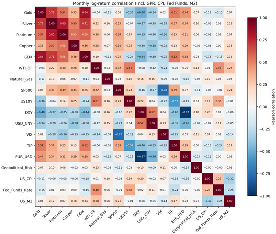
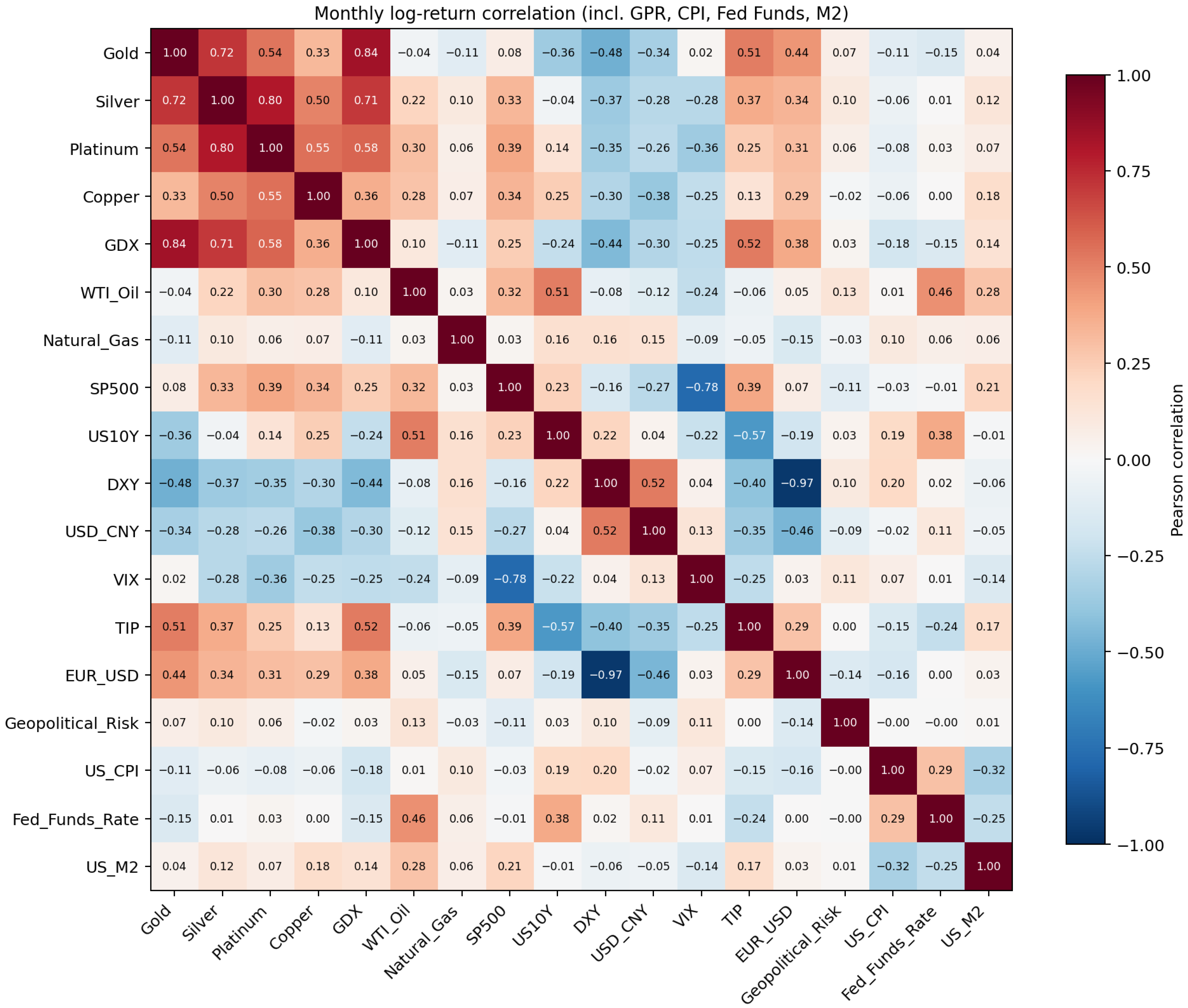
Figure 17 presents the Pearson correlation matrix of monthly log-returns across gold, all commodity and macro-financial predictors, and the four new monetary/geopolitical indicators, confirming the strong contemporaneous co-movement between gold and silver returns (Pearson correlation = 0.70) noted in the prior version and motivating the non-contemporaneous treatment of GDX in the CONTROL set (Section 3.5).

Figure 17. Pearson correlation matrix of monthly log-returns, including GPR, CPI, federal funds rate, and M2.

4.6. Bootstrap Stability of the Cross-Validation Metric

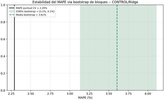
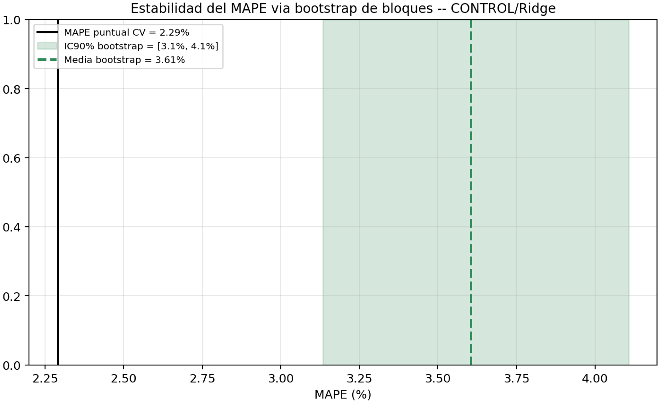
To assess how sensitive the reported cross-validation MAPE is to the specific months in each validation fold, a moving-block bootstrap (block length 3, 2000 replications) was applied to the pooled out-of-sample residuals. The resulting 90% confidence interval for the CV MAPE is [3.13%, 4.11%], compared to the point estimate of 2.29% obtained from the single realized partition (Figure 18). This wider interval indicates that the point estimate carries more sampling uncertainty than its single value suggests and is reported here for transparency rather than presenting a single number that would imply a false sense of precision.

Figure 18. Block-bootstrap distribution of the cross-validation MAPE, CONTROL/Ridge.

4.7. Rolling-Window Evaluation and Volatility Diagnostics

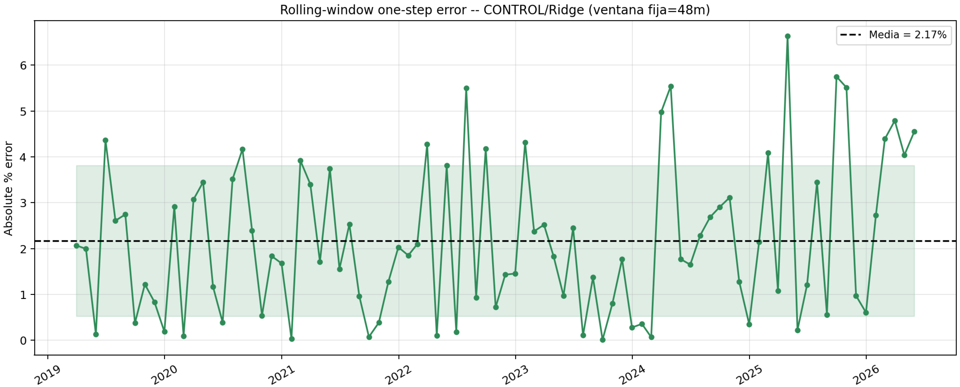
As a further, complementary stability check distinct from the expanding-window cross-validation used for model selection (Section 3.8), a fixed 48-month rolling window was slid one month at a time across the full 2020–2026 sample, refitting CONTROL/Ridge at each step and recording the one-step-ahead absolute percentage error. Across 87 such refits, the mean rolling MAPE is 2.17% (median 1.84%, standard deviation 1.64%), broadly consistent with the cross-validation and bootstrap estimates above and with no visually evident degradation over time (Figure 19).

Figure 19. Rolling-window (48-month fixed window) one-step-ahead error, CONTROL/Ridge.

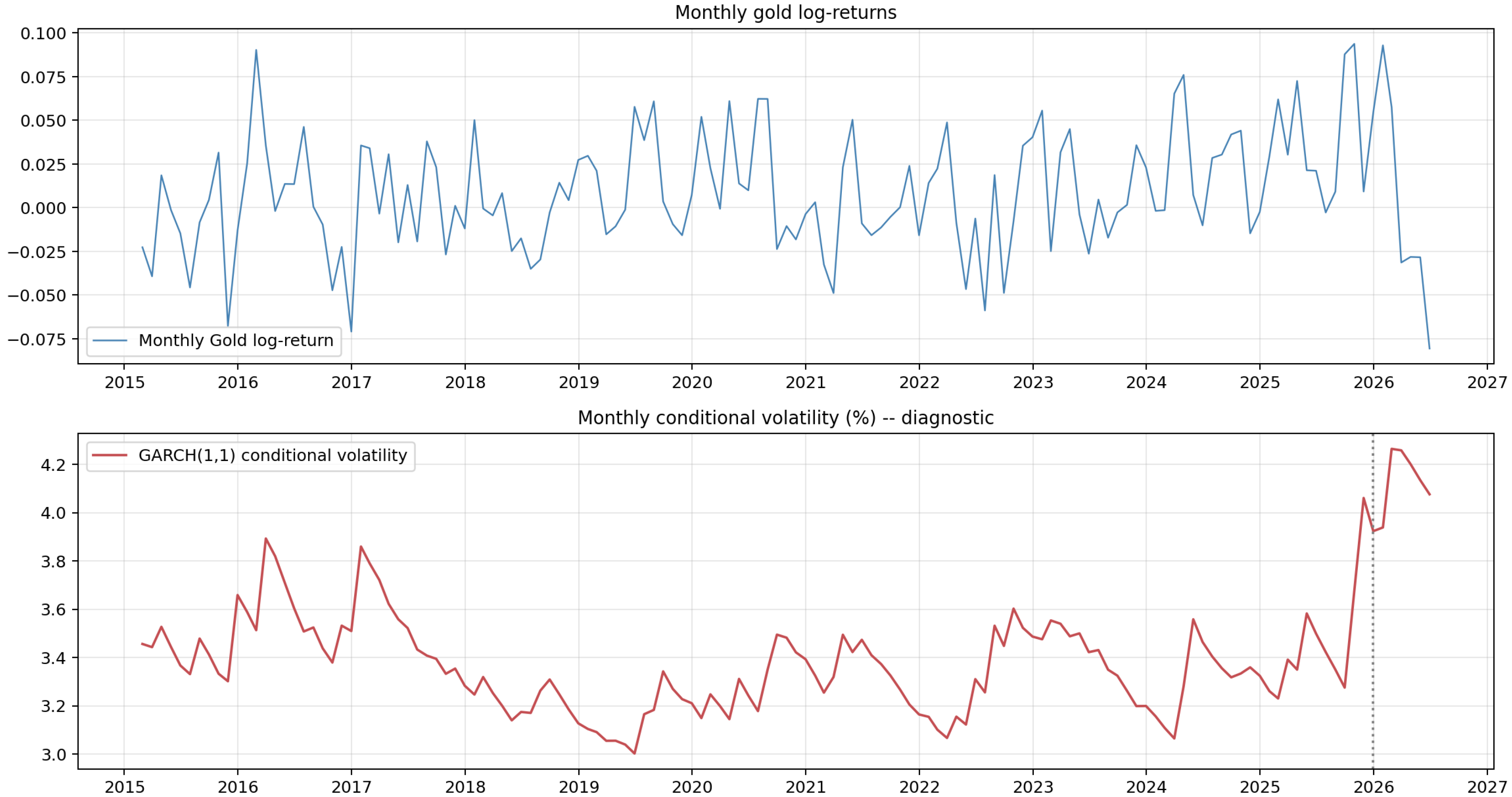
Figure 20 presents the GARCH(1,1) conditional-volatility diagnostic for monthly gold log-returns, characterizing time-varying volatility clustering. As reported in Section 3.11, the Chow test applied to the auxiliary REDUCED-feature regression rejects coefficient stability at the January 2024 candidate break date (F = 2.86, p = 0.006), consistent with the elevated-volatility regime visible in the conditional-volatility series from approximately 2024 onward.

Figure 20. GARCH(1,1) conditional volatility diagnostic for monthly gold log-returns.

4.8. Monte Carlo Forecast and Distributional Robustness

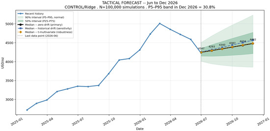
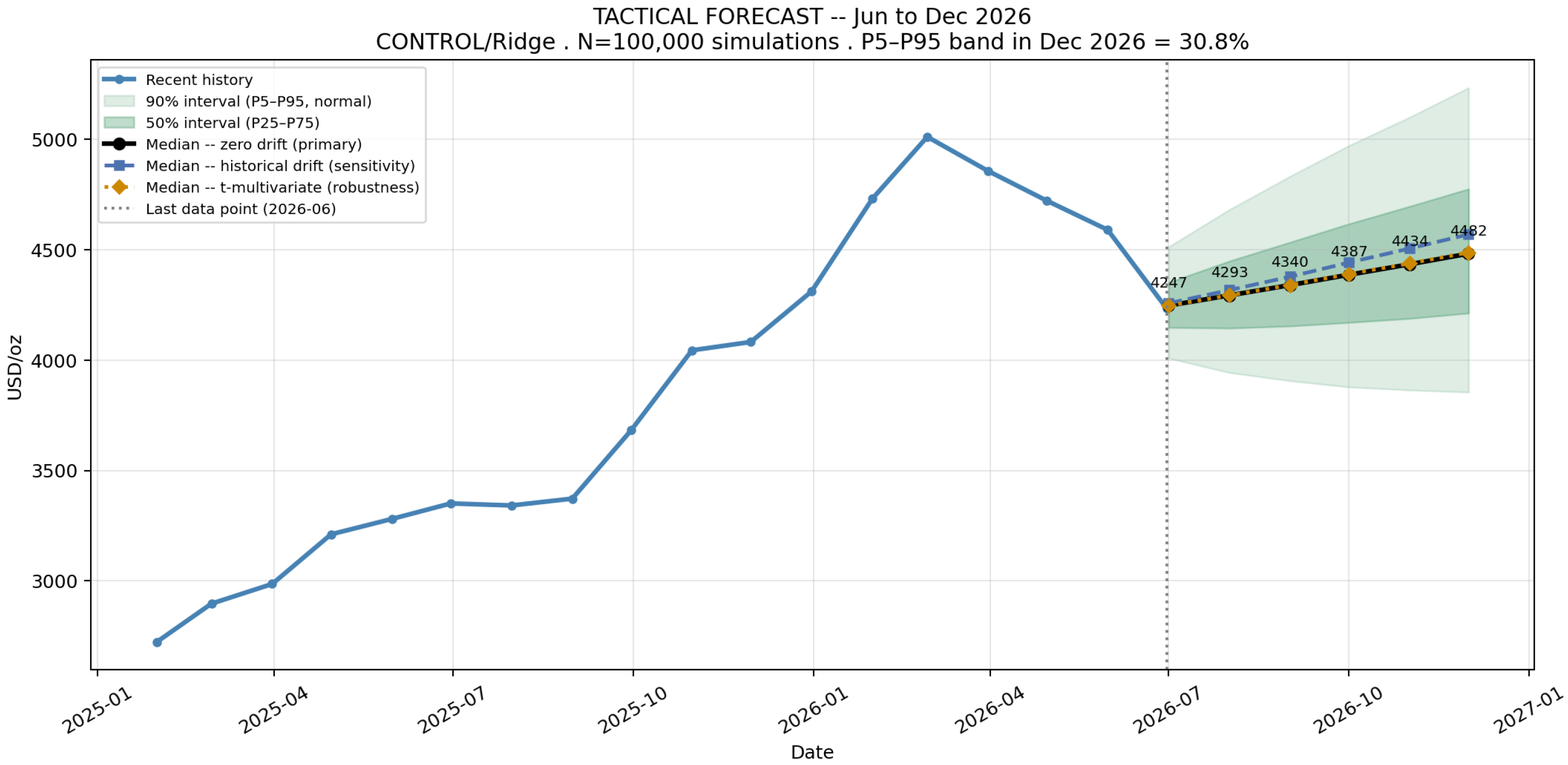
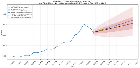
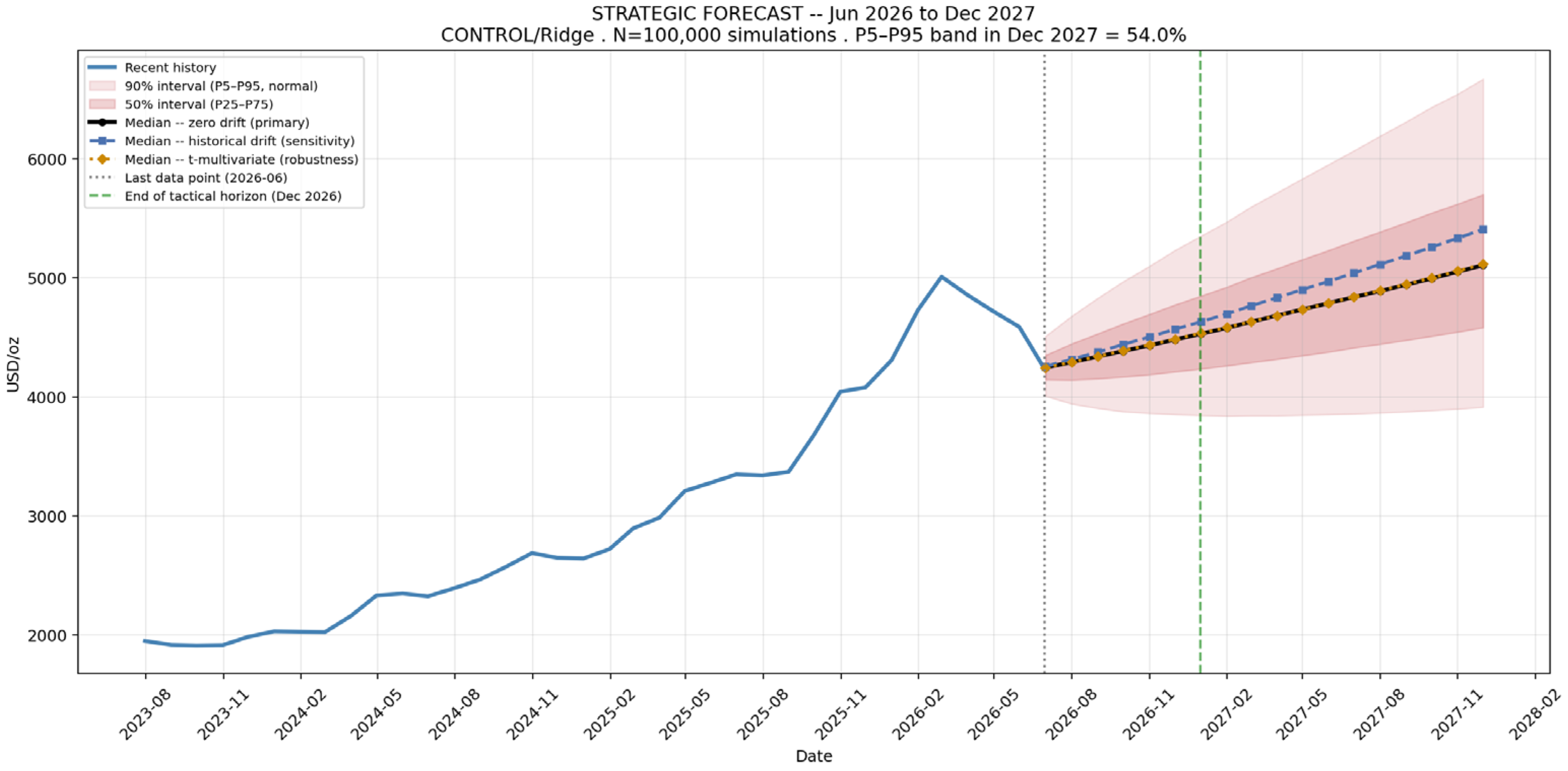
Figure 21 plots the historical gold price series together with the tactical forecast (Objective 2: optimal sales-timing horizon, June–December 2026), and Figure 22 visualizes the full strategic horizon (Objective 3, June 2026–December 2027). Under the primary zero-drift, normal-shock scenario, the tactical horizon projects a median gold price of USD 4482/oz (+5.8% relative to the last observed price), with a 90% interval (P5–P95) spanning approximately 31% of the median. The strategic horizon projects a median of USD 5106/oz (+20.6%), with a 90% interval spanning approximately 54% of the median. The historical-drift sensitivity scenario projects a higher median of USD 5409/oz for December 2027.

Figure 21. Tactical forecast, June–December 2026 (Objective 2: optimal sales-timing horizon).

Figure 22. Strategic forecast, June 2026–December 2027 (Objective 3: long-horizon planning).

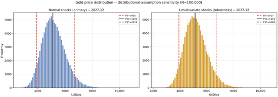
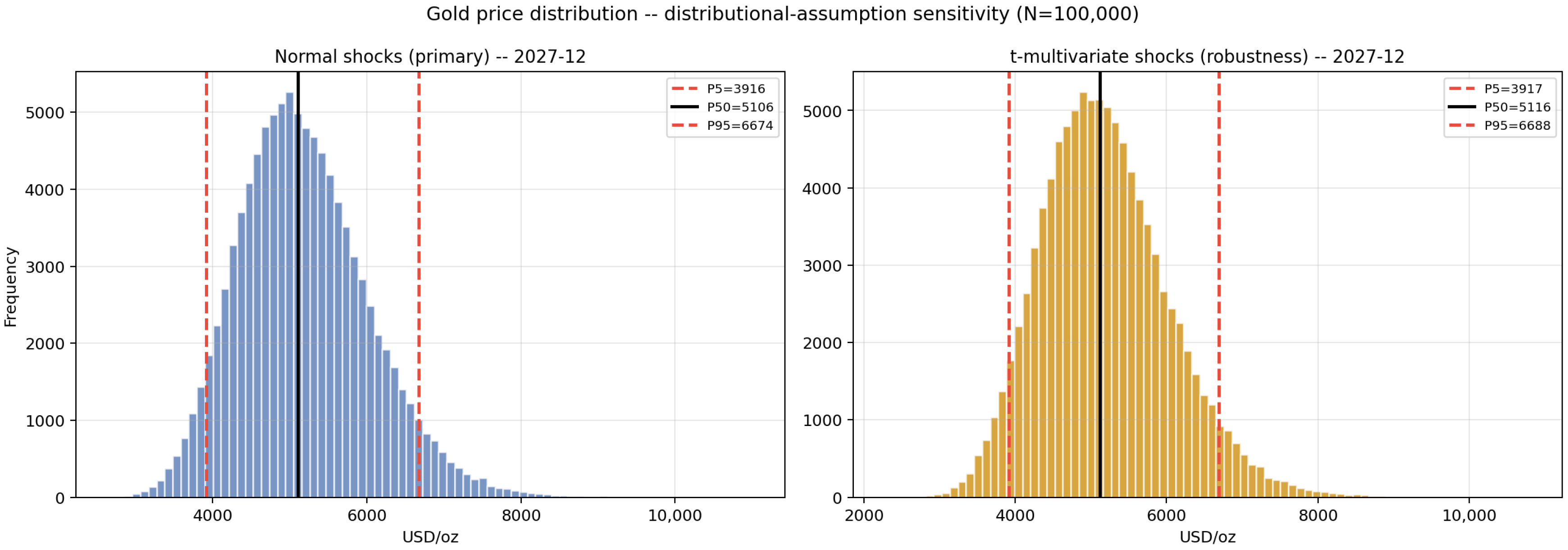
Figure 23 displays the full simulated distribution of gold prices for December 2027 under both the normal-shock and the heavy-tailed (multivariate Student-t) scenarios described in Section 3.10. Under the heavy-tailed robustness scenario, the December 2027 median (USD 5116/oz) is essentially unchanged relative to the normal-shock scenario, and the 90% uncertainty band is only marginally wider (+0.5%). This indicates that, for this particular predictor panel and horizon, the choice between a normal and a heavy-tailed shock distribution has limited practical consequence for the width of the forecast band, a reassuring robustness finding reported transparently rather than assumed.

Figure 23. Simulated distribution of gold price in December 2027, normal vs. multivariate Student-t shocks (N = 100,000 simulations).

As an additional, model-agnostic cross-check of the Monte Carlo uncertainty bands, a split-conformal interval (90% target coverage) and a quantile regression forest were estimated on the same test data. Both produce bands of broadly comparable width to the Monte Carlo P5–P95 interval for the corresponding months, though the conformal interval, calibrated on only six observations, should be regarded as exploratory rather than a definitive alternative to the simulation-based bands.

4.9. Sales-Timing Backtest

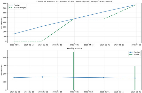
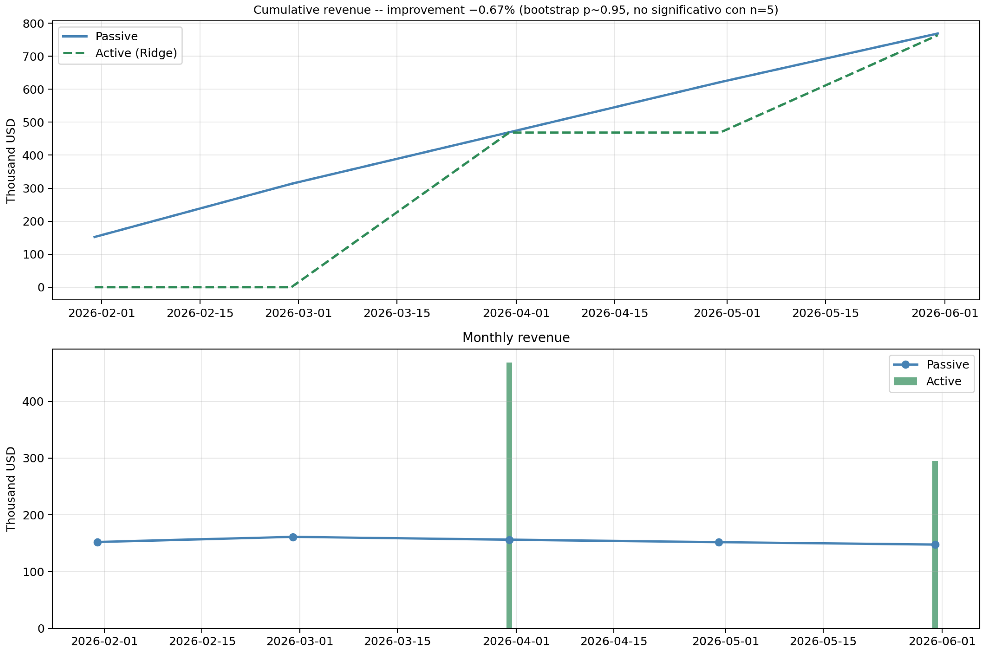
The sales-timing backtest over the official test window (January–May 2026, five commercialization decisions) shows a passive-strategy revenue of USD 768,710.73 against an active-strategy revenue of USD 763,532.59, a difference of −0.67% (Figure 24). A bootstrap test (2000 resamples of the five monthly revenue pairs) estimates that a difference this large, in either direction, would occur by chance with probability approximately 0.95 under the null of no true difference between strategies. This confirms formally what the point estimate alone suggests: with only five sales-timing decisions, the observed underperformance is not statistically distinguishable from zero and should not be read as evidence that the active strategy is worse (or better) than the passive one in a way that would generalize beyond this specific five-month window. Section 5 discusses the economic, as opposed to purely statistical, interpretation of this result in more detail.

Figure 24. Cumulative and monthly revenue, active vs. passive sales-timing strategy.

5. Discussion

5.1. Forecast Accuracy Without Overstated Trading Value

The production model improves one-month-ahead price-forecast accuracy relative to naive alternatives in point-accuracy terms (Section 4.3), yet, as shown in Section 4.9, this improved accuracy does not translate into a statistically distinguishable sales-timing advantage over a simple passive strategy within the available test window. This gap between forecast accuracy and trading value plausibly reflects at least three factors. First, the test period is short (five to ten months), limiting the number of independent timing decisions and the statistical power of any comparison, as formalized by the bootstrap test in Section 4.9. Second, the active-strategy decision rule (comparing the model’s prediction to 101% of a three-month rolling average) is a single, fixed threshold rather than a rule optimized for economic value net of transaction costs; alternative thresholds or a cost-aware decision rule might realize more of the model’s forecast accuracy as economic value, a direction identified for future work (Section 6). Third, accurate point forecasts do not automatically imply correct classification of the specific up/down timing decisions that generate trading value, particularly when the forecast error, while small in percentage terms, is comparable in magnitude to the month-to-month price changes being timed. The result is reported as an honest, neutral finding rather than either overstated success or a reason to discard the model: it provides ASM enterprises with well-calibrated price and uncertainty information (Section 4.8) even though it does not, on this evidence, provide a demonstrated tactical timing edge.

The practical value of the model for ASM enterprises is therefore better framed as conditional rather than universal. Three conditions appear most likely to support meaningful practical value. First, value is more plausible during periods of elevated volatility and regime change, such as the structural break identified around January 2024 (Section 3.11), when the magnitude of month-to-month price movements is large relative to the model’s typical 2–4% forecast error; in the calmer, narrower price ranges more characteristic of the official test window, that same error is comparable in size to the movements being timed, which is consistent with the neutral backtest result reported here. Second, value is more plausible when the model is used for downside risk management, using the Monte Carlo uncertainty bands (Section 4.8) to avoid unfavorable extreme-tail sales outcomes, than when it is used to pursue month-to-month tactical alpha against a passive strategy; the bootstrap-confirmed absence of a timing edge (Section 4.9) does not preclude value as a hedging or planning tool over the longer tactical and strategic horizons (Section 4.8), where the forecast bands remain informative for inventory and sales-scheduling decisions even without a demonstrated short-horizon trading advantage. Third, value would likely increase if the fixed, non-cost-optimized decision rule used in this backtest (Section 4.9) were replaced by a threshold that explicitly accounts for the transaction costs and minimum sale volumes typical of small-scale operations, so that the signal only triggers a deferred sale when the expected gain exceeds those costs by a sufficient margin; this cost-aware refinement is identified as a priority direction for future work (Section 6).

5.2. External Validity and the Global Nature of Gold Prices

Although the study’s motivation centers on Peruvian artisanal mining, every predictor in the model is a global financial variable, which raises the question of whether the practical applicability of the model to the Peruvian mining sector is fully demonstrated. This is a fair description of the model’s scope, but the natural remedy, introducing a Peru-specific variable (such as the USD/PEN exchange rate or local production costs) into the price-determination model itself, is not adopted for a conceptual reason rather than a data-availability one: the gold price is set in global USD markets by global macro-financial conditions, and no Peruvian variable has a theoretical channel through which it would move the world price of gold. Including such a variable in the forecasting model would not improve its external validity; it would introduce a predictor without theoretical justification, working against the correlation–causation discipline established in Section 2.4. The model’s applicability to Peruvian ASM enterprises operates instead through the use case, translating a well-calibrated global-price forecast and its associated uncertainty band into a local sales-timing decision (Section 4.9), rather than through the inclusion of Peru-specific variables in the price model itself. A downstream module that converts the USD/oz forecast into PEN-denominated revenue net of local production costs, using the USD/PEN exchange rate and, where available, local cost indices, is identified as a natural extension of the application layer and is listed as future work in Section 6.

5.3. On the Choice of Monthly Frequency and the Unchanged Title

As detailed in Section 3.2, the monthly sampling frequency is retained because several predictors are natively monthly and because the ASM sales-timing decision this study supports is itself monthly. As detailed in the note under the manuscript title, the title itself remains unchanged for an institutional, not a substantive, reason.

6. Conclusions

This study developed and validated a machine learning system for monthly gold price forecasting in support of ASM sales-timing decisions in Peru, combining an expanded macro-financial and geopolitical predictor set, a broad model and benchmark comparison, formal statistical testing, interpretability tooling, and robustness diagnostics.

Read economically rather than purely statistically, these results indicate that the opportunity-cost and risk-appetite channels captured by the 10-year Treasury yield and the S&P 500 (Section 2.1 and Section 4.5) carry the dominant measurable predictive content for monthly gold returns over the present sample, while the geopolitical and monetary channels, though theoretically plausible (Section 2.1), do not add measurable incremental information once those two channels and commodity co-movements are accounted for. The essentially neutral sales-timing result (Section 4.9) is best interpreted, in economic terms, as evidence that the narrow monthly price differentials relevant to ASM commercialization decisions are not yet reliably exploitable from price information alone, consistent with the mean-reverting, regime-dependent behavior of the real gold price documented by Erb and Harvey (2013), rather than as a failure of the forecasting model itself.

Future research lines should pursue the following directions:

A vector error-correction model (VECM) extension incorporating the four Johansen cointegrating relationships identified in Section 3.4 as an additional predictor, which could improve forecasts at horizons beyond one month while preserving the present framework’s interpretability.

As daily frequency, multi-decade datasets become available, LSTM, state-space, and Markov-switching architectures could be evaluated under the same leakage-free, temporally validated protocol established in this study; these were considered and not implemented on documented sample-size grounds (Section 3.7 and Section 3.2).

The sales-timing backtest should be extended over longer horizons and enriched with transaction-cost-aware decision rules and alternative signal thresholds before any claim of a tactical timing advantage is advanced (Section 5.1).

The integration of textual sentiment indices from financial news sources represents a promising avenue for improving short-horizon predictive precision within the same validated, leakage-free framework.

A panel-data analysis comparing country-specific outcomes (export revenue, production volume, or mining-sector profitability) across gold-exporting economies represents a valuable extension, distinct in scope from the present study’s objective of forecasting the global gold price; a panel-data design, rather than the single-series approach used here, would be the appropriate framework for a country-specific dependent variable.

A downstream, PEN-denominated profitability module, translating the USD/oz forecast and its uncertainty band into local revenue net of production costs via the USD/PEN exchange rate, as discussed in Section 5.2.

A more robust long-memory estimator (e.g., detrended rescaled-range analysis or a wavelet-based estimator), applied to higher-frequency gold-return data, to obtain a more reliable Hurst-exponent estimate than the exploratory result reported in Section 3.11.

References

- Banco Central de Reserva del Perú [BCRP]. (2025). Reporte de inflación, marzo 2025. Available online: https://www.bcrp.gob.pe/docs/Publicaciones/Reporte-Inflacion/2025/marzo/reporte-de-inflacion-marzo-2025.pdf (accessed on 12 January 2026).
- Bauer, M. D., & Hamilton, J. D. (2018). Robust bond risk premia. The Review of Financial Studies, 31(2), 399–448. [Google Scholar] [CrossRef] [Scilit]
- Bollerslev, T. (1986). Generalized autoregressive conditional heteroskedasticity. Journal of Econometrics, 31(3), 307–327. [Google Scholar] [CrossRef] [Scilit]
- Box, G. E. P., Jenkins, G. M., Reinsel, G. C., & Ljung, G. M. (2015). Time series analysis: Forecasting and control (5th ed.). Wiley. Available online: https://www.wiley.com/en-us/Time+Series+Analysis:+Forecasting+and+Control,+5th+Edition-p-9781118675021 (accessed on 12 January 2026).
- Breiman, L. (2001). Random forests. Machine Learning, 45(1), 5–32. [Google Scholar] [CrossRef] [Scilit]
- Brockwell, P. J., & Davis, R. A. (2016). Introduction to time series and forecasting (3rd ed.). Springer. [Google Scholar] [CrossRef] [Scilit]
- Caldara, D., & Iacoviello, M. (2022). Measuring geopolitical risk. American Economic Review, 112(4), 1194–1225. [Google Scholar] [CrossRef] [Scilit]
- Campbell, J. Y., & Thompson, S. B. (2008). Predicting excess stock returns out of sample: Can anything beat the historical average? The Review of Financial Studies, 21(4), 1509–1531. [Google Scholar] [CrossRef] [Scilit]
- Castillo, O. A. (2022). Desarrollo de modelos predictivos de regresión en la industria minera mediante el uso de algoritmo de machine learning [Bachelor’s thesis, Universidad Nacional Mayor de San Marcos]. Cybertesis UNMSM. Available online: https://cybertesis.unmsm.edu.pe/handle/20.500.12672/18458 (accessed on 13 January 2026).
- Clark, T. E., & West, K. D. (2007). Approximately normal tests for equal predictive accuracy in nested models. Journal of Econometrics, 138(1), 291–311. [Google Scholar] [CrossRef] [Scilit]
- Cohen, G., & Aiche, A. (2023). Forecasting gold price using machine learning methodologies. Chaos, Solitons & Fractals, 175, 114079. [Google Scholar] [CrossRef] [Scilit]
- Cont, R. (2001). Empirical properties of asset returns: Stylized facts and statistical issues. Quantitative Finance, 1(2), 223–236. [Google Scholar] [CrossRef]
- CooperAccion. (2024). La marcha de la economía y la minería. Available online: https://cooperaccion.org.pe/economia-y-mineria-20/ (accessed on 13 January 2026).
- Cotrina-Teatino, M. A., Riquelme Sandoval, A. I., Guartán Medina, J. A., & Marquina Araujo, J. J. (2025). Machine learning aplicado a la exploración minera usando matriz de confusión. Sciendo Ingenium, 21(1), 63–74. [Google Scholar] [CrossRef] [Scilit]
- Diaz-Hernandez, A., Ramírez Sánchez, J. C., & Salazar Flores, Y. (2020). Los determinantes de las variaciones en el rendimiento del oro. Contaduría y Administración, 65(2), e169. [Google Scholar] [CrossRef] [Scilit]
- Diebold, F. X. (2015). Forecasting in economics, business, finance and beyond. University of Pennsylvania. Available online: https://www.sas.upenn.edu/~fdiebold/Textbooks.html (accessed on 13 January 2026).
- Diebold, F. X., & Mariano, R. S. (1995). Comparing predictive accuracy. Journal of Business and Economic Statistics, 13(3), 253–263. [Google Scholar] [CrossRef] [Scilit]
- Engle, R. F., & Granger, C. W. J. (1987). Co-integration and error correction: Representation, estimation, and testing. Econometrica, 55(2), 251–276. [Google Scholar] [CrossRef] [Scilit]
- Erb, C. B., & Harvey, C. R. (2013). The golden dilemma. Financial Analysts Journal, 69(4), 10–42. [Google Scholar] [CrossRef] [Scilit]
- Foroutan, P., & Lahmiri, S. (2024). Deep learning systems for forecasting the prices of crude oil and precious metals. Financial Innovation, 10(1), 111. [Google Scholar] [CrossRef] [Scilit]
- Ghule, S., & Gadhave, V. (2022). Gold price prediction using machine learning. International Journal of Scientific Research in Engineering and Management, 6(6), 1–8. [Google Scholar] [CrossRef] [Scilit]
- Gneiting, T., & Katzfuss, M. (2014). Probabilistic forecasting. Annual Review of Statistics and Its Application, 1, 125–151. [Google Scholar] [CrossRef] [Scilit]
- Granger, C. W. J. (1969). Investigating causal relations by econometric models and cross-spectral methods. Econometrica, 37(3), 424–438. [Google Scholar] [CrossRef] [Scilit]
- Gu, S., Kelly, B., & Xiu, D. (2020). Empirical asset pricing via machine learning. The Review of Financial Studies, 33(5), 2223–2273. [Google Scholar] [CrossRef] [Scilit]
- Hamilton, J. D. (1994). Time series analysis. Princeton University Press. Available online: https://press.princeton.edu/books/hardcover/9780691042893/time-series-analysis (accessed on 13 January 2026).
- Hansen, P. R., Lunde, A., & Nason, J. M. (2011). The model confidence set. Econometrica, 79(2), 453–497. [Google Scholar] [CrossRef] [Scilit]
- Harvey, D., Leybourne, S., & Newbold, P. (1998). Tests for forecast encompassing. Journal of Business and Economic Statistics, 16(2), 254–259. [Google Scholar] [CrossRef] [Scilit]
- Hastie, T., Tibshirani, R., & Friedman, J. (2009). The elements of statistical learning: Data mining, inference, and prediction (2nd ed.). Springer. [Google Scholar] [CrossRef]
- Jimenez Falcón, J. B. (2025). Análisis comparativo de algoritmos de aprendizaje automático para la predicción del precio de los minerales en la Bolsa de Valores de Nueva York, 2024 [Bachelor’s thesis, Universidad José Carlos Mariátegui]. Repositorio Institucional UJCM. Available online: https://repositorio.ujcm.edu.pe/handle/20.500.12819/3461 (accessed on 13 January 2026).
- Johansen, S. (1991). Estimation and hypothesis testing of cointegration vectors in Gaussian vector autoregressive models. Econometrica, 59(6), 1551–1580. [Google Scholar] [CrossRef] [Scilit]
- Kelly, B., Pruitt, S., & Su, Y. (2019). Characteristics are covariances: A unified model of risk and return. Journal of Financial Economics, 134(3), 501–524. [Google Scholar] [CrossRef] [Scilit]
- Khani, M., Vahidnia, S., & Abbasi, A. (2021). A deep learning-based method for forecasting gold price with respect to pandemics. SN Computer Science, 2, 393. [Google Scholar] [CrossRef] [Scilit] [PubMed]
- Liang, Y., Lin, Y., & Lu, Q. (2022). Forecasting gold price using a novel hybrid model with ICEEMDAN and LSTM-CNN-CBAM. Expert Systems with Applications, 206, 117847. [Google Scholar] [CrossRef] [Scilit]
- Makridakis, S., Spiliotis, E., & Assimakopoulos, V. (2020). The M4 competition: 100,000 time series and 61 forecasting methods. International Journal of Forecasting, 36(1), 54–74. [Google Scholar] [CrossRef] [Scilit]
- Makridakis, S., Spiliotis, E., & Assimakopoulos, V. (2022). M5 accuracy competition: Results, findings, and conclusions. International Journal of Forecasting, 38(4), 1346–1364. [Google Scholar] [CrossRef] [Scilit]
- Medeiros, M. C., Vasconcelos, G. F. R., Veiga, Á., & Zilberman, E. (2021). Forecasting inflation in a data-rich environment: The benefits of machine learning methods. Journal of Business and Economic Statistics, 39(1), 98–119. [Google Scholar] [CrossRef] [Scilit]
- O’Connor, F. A., Lucey, B. M., Batten, J. A., & Baur, D. G. (2015). The financial economics of gold: A survey. International Review of Financial Analysis, 41, 186–205. [Google Scholar] [CrossRef] [Scilit]
- Ramirez Martínez, C. K. (2017). Determinantes económicas-financieras del precio del oro de 1987 a 2016: Una propuesta usando redes neuronales [Master’s thesis, Universidad Nacional Autónoma de México]. Repositorio Institucional UNAM. Available online: https://repositorio.unam.mx/contenidos/3507368 (accessed on 14 January 2026).
- Rapach, D. E., Strauss, J. K., & Zhou, G. (2010). Out-of-sample equity premium prediction: Combination forecasts and links to the real economy. The Review of Financial Studies, 23(2), 821–862. [Google Scholar] [CrossRef] [Scilit]
- Rumbo Minero. (2024). Producción nacional de oro de enero a octubre del 2024. Available online: https://www.rumbominero.com/peru/noticias/mineria/produccion-nacional-de-oro/ (accessed on 14 January 2026).
- Sadorsky, P. (2021). Predicting gold and silver price direction using tree-based classifiers. Journal of Risk and Financial Management, 14(5), 198. [Google Scholar] [CrossRef] [Scilit]
- Salazar Herrada, E. (2024). Exportaciones de oro peruano se disparan 32% al primer semestre por cotización récord de US$2.205 la onza. Infobae. Available online: https://www.infobae.com/peru/2024/09/11/rally-imparable-del-oro-peruano-exportaciones-se-disparan-32-al-primer-semestre-por-cotizacion-record-de-us2205-la-onza/ (accessed on 14 January 2026).
- Sandoval, L. (2019). Machine learning algorithms for analysis and data prediction. In Proceedings of the IEEE 37th Central America and Panama Convention (CONCAPAN XXXIX), Managua, Nicaragua, November 15–17. IEEE. [Google Scholar] [CrossRef] [Scilit]
- Stock, J. H., & Watson, M. W. (2002). Macroeconomic forecasting using diffusion indexes. Journal of Business and Economic Statistics, 20(2), 147–162. [Google Scholar] [CrossRef] [Scilit]
- Tebin, W., & James, A. (2022, June 15). Gold price prediction using machine learning. National Conference on Emerging Computer Applications (NCECA) (Vol. 4), Kanjirappally, India. [Google Scholar] [CrossRef]
- Tsay, R. S. (2010). Analysis of financial time series (3rd ed.). Wiley. [Google Scholar] [CrossRef] [Scilit]
- Varian, H. R. (2014). Big data: New tricks for econometrics. Journal of Economic Perspectives, 28(2), 3–28. [Google Scholar] [CrossRef] [Scilit]
- Villada, F., Muñoz, N., & García-Quintero, E. (2016). Redes neuronales artificiales aplicadas a la predicción del precio del oro. Información Tecnológica, 27(5), 143–150. [Google Scholar] [CrossRef] [Scilit]
- Wagh, A., Shetty, S., Soman, A., & Maste, D. (2022). Gold price prediction system. International Journal for Research in Applied Science & Engineering Technology, 10(4), 2843–2848. [Google Scholar] [CrossRef] [Scilit]
- West, K. D. (1996). Asymptotic inference about predictive ability. Econometrica, 64(5), 1067–1084. [Google Scholar] [CrossRef] [Scilit]
- Zhang, G., Patuwo, B. E., & Hu, M. Y. (1998). Forecasting with artificial neural networks: The state of the art. International Journal of Forecasting, 14(1), 35–62. [Google Scholar] [CrossRef] [Scilit]
Disclaimer/Publisher’s Note: The statements, opinions and data contained in all publications are solely those of the individual author(s) and contributor(s) and not of MDPI and/or the editor(s). MDPI and/or the editor(s) disclaim responsibility for any injury to people or property resulting from any ideas, methods, instructions or products referred to in the content. |
© 2026 by the authors. Licensee MDPI, Basel, Switzerland. This article is an open access article distributed under the terms and conditions of the Creative Commons Attribution (CC BY) license.